Coupled oscillator model of a trapped Fermi gas at the BEC-BCS crossover

Résumé

We address theoretically the puzzling discontinuity of the radial quadrupole mode frequency observed in a trapped Fermi gas across the BEC-BCS crossover. We apply the scaling transformation to a two-channel model of a resonant Fermi superfluid and argue that the frequency downshift in the crossover region is due to Feshbach coupling of the molecular Bose-Einstein condensate (BEC) to the surrounding Fermi sea. The Bose and Fermi components of the gas act as coupled macroscopic oscillators. The frequency jump corresponds to the point where the closed-channel molecules are entirely converted into the Fermi sea. This implies linear scaling of the "critical" detuning between the scattering channels with the Fermi energy, which can be readily verified in an experiment.

In ultra-cold atomic gases, collective oscillations are key observables that can be measured with high precision Pitaevskii and Stringari (2016). Such measurements offer a unique opportunity to test subtile aspects of the theory. For fermions, the central issue has been the crossover from a weakly-paired Bardeen-Cooper-Schrieffer (BCS) superfluid to a Bose-Einstein condensate (BEC) of tightly bound molecules upon increasing the strength of two-body attraction Gurarie and Radzihovsky (2007); Giorgini et al. (2008); Andreev (2022) . The attractive interaction of atoms can be tuned at will by means of the Feshbach resonance Chin et al. (2010). A widely held conviction is that BEC-BCS crossover connects relevant characteristics of an equilibrium system in a continuous manner. In particular, the spectrum of elementary excitations has been expected to evolve smoothly between the predictions of the hydrodynamic theory of superfluids (BEC side) and the collisionless limit (BCS side) Pitaevskii and Stringari (2016); Combescot et al. (2006). The series of experimental studies outlined below has cast doubt on this belief and posed a challenge to the theory.

Atomic clouds were prepared in axisymmetric harmonic traps in the elongated ($\omega_{z}\ll\omega_{r}$) Altmeyer et al. (2007) and flat ($\omega_{z}\gg\omega_{r}$) Vogt et al. (2012) geometries. The low-energy collective oscillations in this case take the form of discretized normal modes classified by the projection $l_{z}$ of the angular momentum on the symmetry axis ($z$-axis). Of particular interest is the quadrupole mode ($l_{z}=\pm 2$) which corresponds to shape oscillations of the cloud and does not depend on the equation of state Pitaevskii and Stringari (2016). In the collisionless limit this mode is analogous to Landau’s zero sound in a uniform Fermi liquid Landau (1957). At zero temperature the frequency of the collisionless quadrupole mode is predicted to be $\omega_{q}=2\omega_{r}$ Pitaevskii and Stringari (2016), where $\omega_{r}$ is the radial trapping frequency. In the hydrodynamic regime (either irrotational or classical), one has $\omega_{q}=\sqrt{2}\omega_{r}$ Stringari (1996); Pitaevskii and Stringari (1998). Contrary to the aforementioned expectations, the experiments Altmeyer et al. (2007); Vogt et al. (2012) have revealed an abrupt jump between these two values as one tunes the strength of attraction and measures a sequence of equilibrium states of the cloud over the entire crossover. Despite several theoretical attempts Zhou et al. (2008); Chiacchiera et al. (2011, 2013); Baur et al. (2013); Dong et al. (2015), the origin of this discontinuity, as well as the concurrent downshift of $\omega_{q}$ upon entering the crossover from the BEC side, has not been understood.

In this work, we provide an explanation of the observed behaviour in the frame of a two-channel model of a resonant Fermi superfluid Gurarie and Radzihovsky (2007); Andreev (2022). The model establishes reference points for the BEC-BCS crossover. From the BEC side, the crossover begins at the two-body unitarity. As one increases the energy of the closed-channel molecule (resonance) with respect to the open channel, the molecular condensate dissociates into fermions which form a BCS ground state. The crossover terminates at the point where the molecules are entirely converted into the fermions: beyond this point, the boson population is exponentially small. Although there is a unique broken $U(1)$ symmetry associated with conservation of the total number of particles over the entire crossover, the model inherently incorporates a fundamental difference between the BEC and BCS condensates. What makes the difference is the non-linearity: whereas Cooper pairs do not interact, the molecules behave as weakly-repulsive bosons. We argue that the respective solutions for $\omega_{q}$ in BEC and BCS phases stem from different dynamical scaling and cannot be connected in a continuous fashion. In the crossover region, the BEC and BCS condensates constitute two distinct macroscopic oscillators coupled to each other via a coherent Feshbach link. The strength of the coupling increases with spatial overlap between the components and buildup of a Fermi surface, as one moves toward the BCS side.

The model Hamiltonian reads

$$\begin{split}\hat{H}(t)=&\int\sum_{\sigma=\uparrow,\downarrow,B}\hat{\Psi}^{\dagger}_{\sigma}(\bm{r},t)\left[-\frac{\hbar^{2}}{2m_{\sigma}}\Delta+V_{\sigma}(\bm{r},t)\right]\hat{\Psi}_{\sigma}(\bm{r},t)d\bm{r}\\ &+\frac{1}{2}\sum_{\sigma,\sigma^{\prime}}\bar{g}_{\sigma\sigma^{\prime}}\int\hat{\Psi}^{{\dagger}}_{\sigma}\hat{\Psi}^{{\dagger}}_{\sigma^{\prime}}\hat{\Psi}_{\sigma^{\prime}}\hat{\Psi}_{\sigma}d\bm{r}+\bar{\delta}\int\hat{\Psi}_{B}^{\dagger}\hat{\Psi}_{B}d\bm{r}\\ &-\alpha\int\hat{\Psi}^{\dagger}_{\uparrow}(\bm{r},t)\hat{\Psi}^{\dagger}_{\downarrow}(\bm{r},t)\hat{\Psi}_{B}(\bm{r},t)d\bm{r}-\mathrm{H.c.},\end{split}$$ (1)

where fermions of equal masses $m_{\uparrow}=m_{\downarrow}\equiv m$ are described by the second-quantized fields $\hat{\Psi}_{\uparrow}(\bm{r},t)$ and $\hat{\Psi}_{\downarrow}(\bm{r},t)$, and the field operator $\hat{\Psi}_{B}(\bm{r},t)$ stands for their bosonic molecules with mass $m_{B}=2m$. We shall neglect thermal and quantum depletion of the molecular condensate and replace $\hat{\Psi}_{B}(\bm{r},t)$ by a classical field $\Psi_{B}(\bm{r},t)$. The effective interactions $\bar{g}_{\sigma\sigma^{\prime}}=2\pi\hbar^{2}/m_{\sigma\sigma^{\prime}}\bar{a}_{\sigma\sigma^{\prime}}$ are defined by the corresponding reduced masses $m_{\sigma\sigma^{\prime}}=m_{\sigma}m_{\sigma^{\prime}}/(m_{\sigma}+m_{\sigma^{\prime}})$ and $s$-wave scattering lengths $\bar{a}_{\sigma\sigma^{\prime}}$, and include the background attraction between the fermions of opposite spins $\bar{g}_{\uparrow\downarrow}<0$. We assume, however, that the pairing is dominated by the Feshbach resonance described by the last two terms. Namely, for a singlet pair of fermions in vacuum, the Hamiltonian (1) yields the scattering length Andreev (2022)

$$a_{\uparrow\downarrow}=\bar{a}_{\uparrow\downarrow}-\pi^{-1}(m/\hbar^{2})\alpha^{2}/\delta.$$ (2)

The parameter $\alpha>0$ is proportional to the microscopic volume of the closed-channel molecule $\upsilon$ and to the Josephson energy associated with the coherent Feshbach coupling (i. e., the hyperfine interaction). We assume $\upsilon^{1/3}\ll\sqrt{\hbar/m\omega_{\mathrm{ho}}}$, where $\omega_{\mathrm{ho}}=\sqrt{\omega_{r}\omega_{z}}$. The renormalized detuning $\delta=\bar{\delta}+\delta_{\alpha}$ is reduced with respect to its bare value $\bar{\delta}$ by the amount $\delta_{\alpha}\propto-\alpha^{2}$.

In practice, the bare detuning $\bar{\delta}$ is controlled by the Zeeman splitting between the open and closed channels of the Feshbach resonance. By writing $\delta=\mu_{B}\mathrm{g}(B-B_{0})$ and defining

$$\Delta B\equiv m\alpha^{2}/(\pi\mu_{B}\mathrm{g}\hbar^{2}\bar{a}_{\uparrow\downarrow}),$$ (3)

we may recast the above expression for $a_{\uparrow\downarrow}$ in the familiar form Pitaevskii and Stringari (2016)

$$a_{\uparrow\downarrow}=\bar{a}_{\uparrow\downarrow}\left(1-\frac{\Delta B}{B-B_{0}}\right).$$ (4)

The magnetic field $B=B_{0}$ corresponds to the unitarity, where the scattering length $a_{\uparrow\downarrow}$ diverges. The formulas (3) and (4) establish a link between the model and the experiments.

The bare detuning $\bar{\delta}$ together with the total number of particles

$$N=\int(\braket{\hat{\Psi}_{\uparrow}^{\dagger}\hat{\Psi}_{\uparrow}}+\braket{\hat{\Psi}_{\downarrow}^{\dagger}\hat{\Psi}_{\downarrow}}+2|\Psi_{B}|^{2})d\bm{r}$$ (5)

are the control parameters which define the equilibrium configuration and dynamical properties of the system. For instance, behaviour of the gas in a time-dependent harmonic trap

$$V_{\sigma}(\bm{r},t)=\frac{m_{\sigma}}{2}[\omega_{x}(t)^{2}x^{2}+\omega_{y}(t)^{2}y^{2}+\omega_{z}(t)^{2}z^{2}]$$ (6)

is well understood in the limiting cases $\bar{\delta}<-\delta_{\alpha}$ (BEC regime) Pitaevskii and Stringari (1998); Edwards et al. (1996); Jin et al. (1996); Jochim et al. (2003); Kagan et al. (1996, 1997) and $\bar{\delta}\gg 2\mu$ (BCS regime) Bruun and Clark (2000); Grasso et al. (2005), where $\mu(N)$ is the Fermi energy calculated in that latter limit. The intermediate range $-\delta_{\alpha}<\bar{\delta}\lesssim 2\mu$ corresponds to the BEC-BCS crossover regime addressed in this work.

We shall be interested in the radial quadrupole oscillation of the cloud, which can be triggered, e. g., by a sudden quench of a slightly anizotropic trap $\omega_{x}(0)\neq\omega_{y}(0)$ to the axially symmetric configuration $\omega_{x}(t)=\omega_{y}(t)\equiv\omega_{r}$, the latter then being retained at all times $t>0$. To describe the resulting shape oscillations, we perform the scaling transformation Castin and Dum (1996); Kagan et al. (1996, 1997); Dalfovo et al. (1997); Bruun and Clark (2000)

$$\begin{split}\hat{\Psi}_{\uparrow,\downarrow}(\bm{r},t)&=\frac{1}{\sqrt{\mathcal{V}_{b}(t)}}\hat{\chi}_{\uparrow,\downarrow}[\bm{\rho}(t),\mathsf{t}(t)]e^{i\Phi_{\uparrow,\downarrow}(\bm{r},t)}\\ \Psi_{B}(\bm{r},t)&=\frac{1}{\sqrt{\mathcal{V}_{c}(t)}}\chi_{B}[\bm{\varrho}(t),\mathfrak{t}(t)]e^{i\Phi_{B}(\bm{r},t)}\end{split}$$ (7)

with $\rho_{i}(t)=x_{i}/b_{i}(t)$, $\varrho_{i}(t)=x_{i}/c_{i}(t)$, $\mathcal{V}_{b}(t)=b_{x}(t)b_{y}(t)b_{z}(t)$, $\mathcal{V}_{c}(t)=c_{x}(t)c_{y}(t)c_{z}(t)$ $\mathsf{t}(t)=\int\limits^{t}\mathcal{V}_{b}^{-1}(t^{\prime})dt^{\prime}$, $\mathfrak{t}(t)=\int\limits^{t}\mathcal{V}_{c}^{-1}(t^{\prime})dt^{\prime}$ and the quadratic ansatzes for the phases

$$\begin{split}\Phi_{\uparrow}(\bm{r},t)&=\Phi_{\downarrow}(\bm{r},t)=\frac{m}{2\hbar}\sum_{i=x,y,z}\frac{\dot{b}_{i}}{b_{i}}x_{i}^{2}\\ \Phi_{B}(\bm{r},t)&=\frac{m}{\hbar}\sum_{i=x,y,z}\frac{\dot{c}_{i}}{c_{i}}x_{i}^{2}\;(\mathrm{mod}\>\pi)\end{split}$$ (8)

As a first step, let us neglect the Feshbach coupling between the channels by sending $\alpha\rightarrow 0$. The crossover boundaries in this limit become

$$0<\delta<2\mu,$$ (9)

and one has $\delta=\bar{\delta}$. The equations of motion for the fermionic fields and the molecular condensate order parameter in the new variables read

$$i\hbar\frac{\partial\hat{\chi}_{\uparrow,\downarrow}}{\partial\mathsf{t}} =\left[-\frac{\hbar^{2}}{2m}\sum_{i}\frac{\mathcal{V}_{b}}{b_{i}^{2}}\frac{\partial^{2}}{\partial\rho_{i}^{2}}+\frac{m}{2}\sum_{i}\omega_{0i}^{2}\rho_{i}^{2}+\bar{g}_{FB}|\chi_{B}|^{2}\frac{\mathcal{V}_{b}}{\mathcal{V}_{c}}\right]\hat{\chi}_{\uparrow,\downarrow}$$ (10a)

$$i\hbar\frac{\partial\chi_{B}}{\partial\mathfrak{t}} =\left[-\frac{\hbar^{2}}{4m}\sum_{i}\frac{\mathcal{V}_{c}}{c_{i}^{2}}\frac{\partial^{2}}{\partial\varrho_{i}^{2}}+m\sum_{i}\omega_{0i}^{2}\varrho_{i}^{2}+\bar{g}_{FB}\left(\braket{\hat{\chi}_{\uparrow}^{\dagger}\hat{\chi}_{\uparrow}}+\braket{\hat{\chi}_{\downarrow}^{\dagger}\hat{\chi}_{\downarrow}}\right)\frac{\mathcal{V}_{c}}{\mathcal{V}_{b}}+\bar{g}_{BB}|\chi_{B}|^{2}+\delta\right]\chi_{B},$$ (10b)

where one has

$$\ddot{b}_{i}+\omega_{i}^{2}b_{i} =\frac{\omega_{0i}}{\mathcal{V}_{b}b_{i}^{2}}$$ (11a)

$$\ddot{c}_{i}+\omega_{i}^{2}c_{i} =\frac{\omega_{0i}}{\mathcal{V}_{c}c_{i}^{2}}$$ (11b)

with $\omega_{0i}\equiv\omega_{i}(0)$. Here and in what follows we write the constant quantities having the dimension of energy by using the corresponding units of time. Thus, the detuning $\delta$ in Eq. (10b) has been rescaled by the factor $\mathcal{V}_{c}$. We have also introduced the notation $\bar{g}_{FB}\equiv\bar{g}_{\uparrow B}=\bar{g}_{\downarrow B}$ for the effective interaction of fermions with bosons. Finally, in Eq. (10a) we have omitted the terms $\bar{g}_{\uparrow\downarrow}\braket{\hat{\chi}_{\downarrow}\hat{\chi}_{\uparrow}}\hat{\chi}_{\downarrow,\uparrow}^{\dagger}$ which would be exponentially suppressed in the dilute limit [see Eq. (29) below].

Consider limiting forms of Eqs. (10). First, on the BCS side one has $|\chi_{B}|\equiv 0$ and Eq. (10a) becomes the equation of motion of an ideal Fermi gas in a harmonic trap. By writing $\hat{\chi}_{\uparrow,\downarrow}=\hat{\xi}_{\uparrow,\downarrow}(\rho_{x})\hat{\xi}_{\uparrow,\downarrow}(\rho_{y})\hat{\xi}_{\uparrow,\downarrow}(\rho_{z})$ this equation can be further reduced to three independent equations

$$i\hbar\frac{\partial\hat{\xi}_{\uparrow,\downarrow}}{\partial\tau_{i}}=\left[-\frac{\hbar^{2}}{2m}\frac{\partial^{2}}{\partial\rho_{i}^{2}}+V_{\uparrow,\downarrow}^{(i)}(\rho_{i})\right]\hat{\xi}_{\uparrow,\downarrow}(\rho_{i})$$ (12)

with $\tau_{i}(t)=\int\limits^{t}b_{i}^{-2}(t^{\prime})dt^{\prime}$, $V_{\uparrow,\downarrow}^{(i)}(\rho_{i})=m\omega_{0i}^{2}\rho_{i}^{2}/2$ and

$$\ddot{b}_{i}+\omega_{i}^{2}b_{i}=\frac{\omega_{0i}^{2}}{b_{i}^{3}},$$ (13)

the latter now replacing the coupled equations (11a). Following our protocol for excitation of the quadrupole mode, we write $\omega_{0x}=(1+\mathsf{c})\omega_{r}$ and $\omega_{0y}=(1-\mathsf{c})\omega_{r}$, and look for the solutions of Eq. (13) in the form $b_{i}(t)=1+\delta b_{i}(t)$ with the initial conditions $b_{i}(0)=1$ and $\dot{b}_{i}(0)=0$. Assuming $\mathsf{c}\ll 1$, we obtain

$$\begin{split}\delta b_{x}(t)&=\tfrac{1}{2}\mathsf{c}(1-\cos[\omega_{q}^{(\mathrm{BCS})}t])\\ \delta b_{y}(t)&=-\tfrac{1}{2}\mathsf{c}(1-\cos[\omega_{q}^{(\mathrm{BCS})}t])\end{split}$$ (14)

with

$$\omega_{q}^{(\mathrm{BCS})}=2\omega_{r}.$$ (15)

Finite molecular density $|\chi_{B}|^{2}$ goes as a perturbation to the external harmonic potential and does not prevent Eq. (10a) from factorization. The structure of the final Eq. (12) is preserved. The scaling equation Eq. (13) in the presence of the condensate would take the from of a damped driven harmonic oscillator. The solution is an oscillation with the frequency of the driving force. Detailed argument will be provided below.

In the opposite limit of $\braket{\hat{\chi}_{\uparrow}^{\dagger}\hat{\chi}_{\uparrow}}=\braket{\hat{\chi}_{\downarrow}^{\dagger}\hat{\chi}_{\downarrow}}=0$ (BEC side), one may take advantage of the Thomas-Fermi approximation for the molecular condensate order parameter to obtain a stationary solution of Eq. (10b) in the form $\chi_{B}=|\chi_{B}|e^{-i2\mu\mathfrak{t}}$ and

$$g_{BB}|\chi_{B}(\bm{\varrho})|^{2}=2\mu-\delta-m\sum_{i}\varrho_{i}^{2}\omega_{0i}^{2}.$$ (16)

The positive difference $2\mu-\delta>0$ is defined by the normalization condition (5). Solution of the system of coupled scaling equations (11b), where we put $c_{z}(t)\equiv 1$, yields

$$\begin{split}\delta c_{x}(t)&=\mathsf{c}(1-\cos[\omega_{q}^{(\mathrm{BEC})}t])\\ \delta c_{y}(t)&=-\mathsf{c}(1-\cos[\omega_{q}^{(\mathrm{BEC})}t])\end{split}$$ (17)

with

$$\omega_{q}^{(\mathrm{BEC})}=\sqrt{2}\omega_{r}$$ (18)

and $\mathsf{c}\ll 1$.

Formally, the difference between the BEC [Eq. (18)] and BCS [Eq. (15)] results can be traced back to absence of the non-linear term in Eq. (10a), which allows subsequent factorization of the scaling equations (11a). We now show that both results hold simultaneously within the crossover range (9), where the BEC and BCS condensates coexist. No new oscillation arise and the values of the frequencies $\omega_{q}^{(\mathrm{BCS})}$ and $\omega_{q}^{(\mathrm{BEC})}$ remain intact.

At $0<\delta\ll 2\mu$ we may still use Eq. (16), which we substitute into Eq. (10a) and obtain the factorized form analogous to Eq. (12), where now the external harmonic potential $V_{i}(\rho_{i})$ should be substituted by an effective potential

$$U_{\uparrow,\downarrow}^{(i)}(\rho_{i})=\tfrac{1}{2}m\tilde{\omega}_{0i}^{2}\rho_{i}^{2}+\tfrac{g_{FB}}{g_{BB}}(2\mu-\delta)$$ (19)

in the region of space where Eq. (16) yields non-zero condensate density. Hence, the problem in this region has been reduced to an ideal Fermi gas residing in a superposition of the external potential and an effective mean-field potential produced by the molecular condensate Mølmer (1998). In 3D one has $g_{FB}/g_{BB}\approx 3$ Petrov (2003); Petrov et al. (2004), so that square of the rescaled frequency $\tilde{\omega}_{0i}^{2}=\omega_{0i}^{2}\left(1-\tfrac{2g_{FB}}{g_{BB}}\right)$ is negative and the effective potential (19) has the form of an inverted parabola.

The fermions thus form a shell around the molecular core. The exact form of the fermion density profile can be worked out by using the semiclassical approach Pitaevskii and Stringari (2016). Oscillation of the outer part of the shell, which feels only the external potential, is still governed by Eq. (13). The inner part, which feels the effective potential (19), oscillates according to the modified scaling equations

$$\begin{split}\ddot{b}_{x}+\tilde{\omega}_{x}^{2}b_{x}&=\frac{\tilde{\omega}_{0x}^{2}}{b_{x}^{3}}+\mathsf{c}\tfrac{2g_{FB}}{g_{BB}}[\omega_{q}^{(\mathrm{BEC})}]^{2}\cos[\omega_{q}^{(\mathrm{BEC})}t]\\ \ddot{b}_{y}+\tilde{\omega}_{y}^{2}b_{y}&=\frac{\tilde{\omega}_{0y}^{2}}{b_{y}^{3}}-\mathsf{c}\tfrac{2g_{FB}}{g_{BB}}[\omega_{q}^{(\mathrm{BEC})}]^{2}\cos[\omega_{q}^{(\mathrm{BEC})}t]\end{split}$$ (20)

where $\tilde{\omega}_{i}^{2}=\omega_{i}^{2}\left(1-\tfrac{2g_{FB}}{g_{BB}}\right)<0$ and we have used Eq. (17) for the quadrupole oscillation of the condensate. These are equations of damped driven harmonic oscillators. Their solutions are linear superpositions of the transients

$$\begin{split}\delta b_{x}(t)&=\tfrac{1}{2}\mathsf{c}(1-\exp[-\tilde{\omega}_{q}^{(\mathrm{BCS})}t])\\ \delta b_{y}(t)&=-\tfrac{1}{2}\mathsf{c}(1-\exp[-\tilde{\omega}_{q}^{(\mathrm{BCS})}t]),\end{split}$$ (21)

with $\tilde{\omega}_{q}^{(\mathrm{BCS})}=2|\tilde{\omega}_{r}|$ and oscillations at the frequency of the driven force $\omega_{q}^{(\mathrm{BEC})}$, given by Eq. (18). The driven oscillations of the fermion shell are in-phase with the molecular BEC.

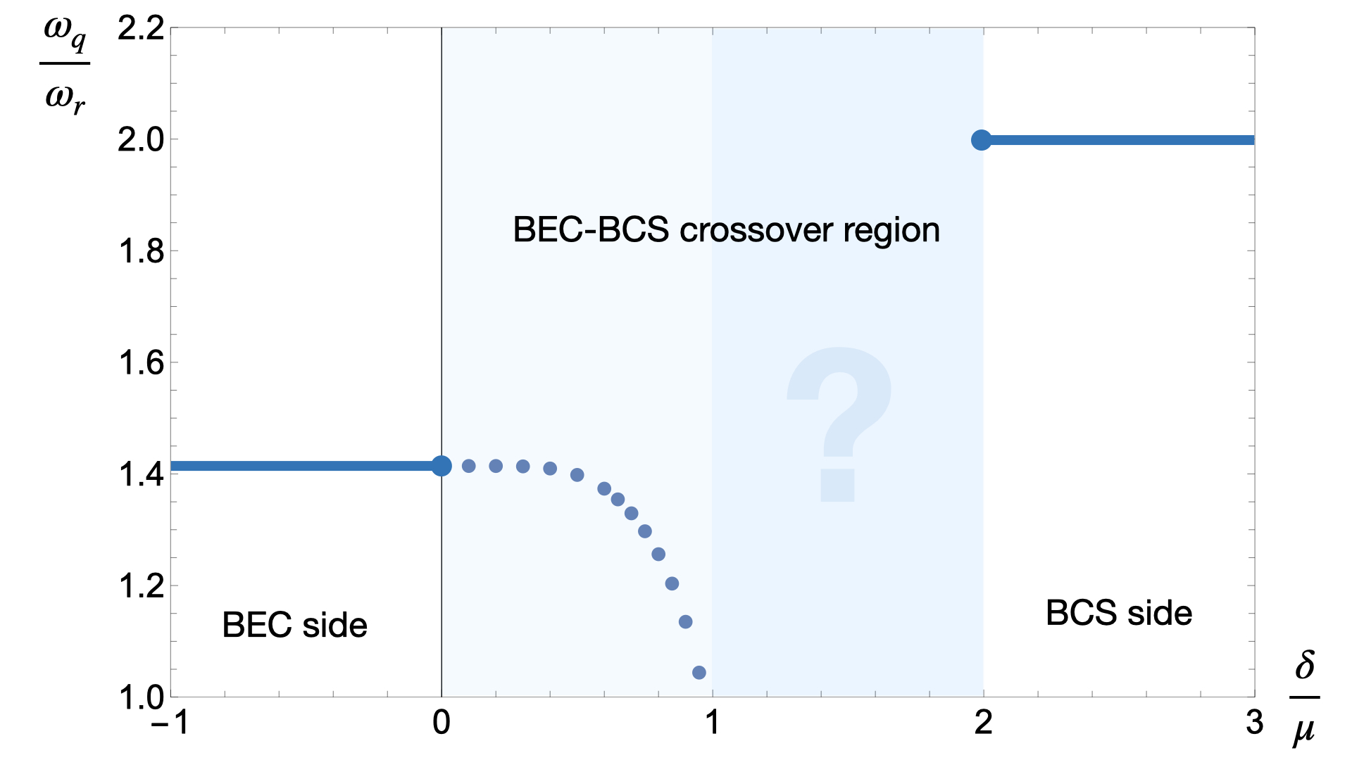
Figure 1: Quadrupole oscillation frequency as a function of the detuning. Solid lines are the exact values obtained within the scaling approach in the BEC [Eq. (18)] and BCS [Eq. (15)] limits. The end-points (large filled circles) mark the BEC-BCS crossover (shaded area) boundaries. The vertical line at $\delta=0$ marks the unitarity. The dots represent the perturbative result (28). We have used the parameters of the experiment Altmeyer et al. (2007). Understanding of behaviour in the doubly-shaded area would require further refinement of the theory.

As the fermion density grows upon increasing $\delta$, the mutual repulsion with the molecular BEC starts to contribute also into Eq. (10b). However, the corresponding effective potential now has positive curvature and, being approximated by a parabola, yields positive square of the rescaled frequency. The oscillator associated with the molecular BEC, although being driven by the fermionic component in the overlap region, is undamped and thus preserves its normal mode . We conclude that, within the Thomas-Fermi approximation, there are two independent modes [Eq. (15) and Eq. (18)] which remain intact over the entire crossover.

We now restore the Feshbach coupling $\alpha$ between the channels and treat it as a perturbation to Eqs. (10). The corresponding corrections to the scaling equations can be worked out by considering dynamics of the average squared radii

$$\braket{\hat{x}_{i}^{2}(t)}_{\sigma}=b_{i}^{2}(t)\braket{\hat{x}_{i}^{2}(0)}_{\sigma}=\frac{1}{N_{\sigma}(t)}\int n_{\sigma}(t)x_{i}^{2}(t)d\bm{r},$$ (22)

($\sigma=\uparrow,\downarrow$) and analogously for $c_{i}^{2}(t)$ ($\sigma=B$). The full time derivative of $\braket{\hat{x}_{i}^{2}(t)}_{\sigma}$ would contain corrections to $\dot{N}_{\sigma}$ and $\dot{n}_{\sigma}$ due to Josephson currents induced by the Feshbach link:

$$\begin{split}\dot{n}_{\uparrow,\downarrow}&=\dot{n}_{\uparrow,\downarrow}^{(0)}+\frac{2\alpha}{\hbar}\sin(\Delta\Phi)|\braket{\hat{\Psi}_{\downarrow}\hat{\Psi}_{\uparrow}}\Psi_{B}^{\ast}|\\ \dot{n}_{B}&=\dot{n}_{B}^{(0)}-\frac{2\alpha}{\hbar}\sin(\Delta\Phi)|\braket{\hat{\Psi}_{\downarrow}\hat{\Psi}_{\uparrow}}\Psi_{B}^{\ast}|,\end{split}$$ (23)

where $n_{\sigma}^{(0)}(t)$ stand for the uncoupled densities and we have defined the relative phase

$$\Delta\Phi\equiv\Phi_{\uparrow}+\Phi_{\downarrow}-\Phi_{B}.$$ (24)

Note, that $\dot{N}_{\sigma}^{(0)}=\int\dot{n}_{\sigma}^{(0)}d\bm{r}=0$. By using Eqs. (8), one may obtain

$$\delta\ddot{b}_{i} =\delta\ddot{b}_{i}^{(0)}+\Gamma_{ii}(\delta\ddot{b}_{i}-\delta\ddot{c}_{i})+\Gamma_{ij}(\delta\ddot{b}_{j}-\delta\ddot{c}_{j})$$ (25a)

$$\delta\ddot{c}_{i} =\delta\ddot{c}_{i}^{(0)}+\Lambda_{ii}(\delta\ddot{c}_{i}-\delta\ddot{b}_{i})+\Lambda_{ij}(\delta\ddot{c}_{j}-\delta\ddot{b}_{j}),$$ (25b)

where $j\neq i$ and expressions for the coupling matrix elements may be found in SI . By virtue of the cylindrical symmetry of the problem, one has $\Gamma_{xx}=\Gamma_{yy}$, $\Gamma_{xy}=\Gamma_{yx}$ and $\Lambda_{xx}=\Lambda_{yy}$, $\Lambda_{xy}=\Lambda_{yx}$. The zeroth-order quantities $\delta\ddot{b}_{i}^{(0)}$ and $\delta\ddot{c}_{i}^{(0)}$ obey the uncoupled scaling equations derived above for $\alpha=0$.

Thus constructed system of coupled differential equations on the scaling parameters does no longer admit a global quadrupole solution which would be compatible with the previously used initial conditions, i. e., $\delta b_{i}(0)=0$, $\delta\dot{b}_{i}(0)=0$ and, simultaneously, $\delta c_{i}(0)=0$, $\delta\dot{c}_{i}(0)=0$. We, therefore, relax our statement of the problem by assuming that only the majority component (the molecular BEC) dynamics is subjected to the initial conditions $\delta c_{i}(0)=0$, $\delta\dot{c}_{i}(0)=0$, whereas the phase and amplitude of the fermion oscillation is defined entirely by the coupling. This is consistent with our above conclusion on the driven nature of the fermion oscillator. Formally, this amounts to reducing the system of four coupled equations (25) to just two coupled equations for the differences $\delta\ddot{b}\equiv\delta\ddot{b}_{x}-\delta\ddot{b}_{y}$ and $\delta\ddot{c}\equiv\delta\ddot{c}_{x}-\delta\ddot{c}_{y}$. By taking $\delta\ddot{b}=\mathsf{b}\omega_{q}^{2}\cos(\omega_{q}t)$, $\delta\ddot{c}=\mathsf{c}\omega_{q}^{2}\cos(\omega_{q}t)$ and assuming $\omega_{q}=\sqrt{2}\omega_{r}+\delta\omega_{q}$ with $\delta\omega_{q}\ll\sqrt{2}\omega_{r}$, we arrive at the eigenvalue problem

$$\left|\begin{array}[]{cc}2\omega_{r}^{2}[1+\Gamma(\delta)]-\omega_{q}^{2}&2\omega_{r}^{2}\Gamma(\delta)\\ 2\omega_{r}^{2}\Lambda(\delta)&2\omega_{r}^{2}[1+\Lambda(\delta)]-\omega_{q}^{2}\end{array}\right|=0,$$ (26)

where

$$\Gamma(\delta)=\frac{\alpha m}{2\hbar^{2}}\cos(\Delta\Phi)\frac{\int\limits_{-\infty}^{+\infty}d\rho_{z}\int\limits_{0}^{+\infty}|\braket{\hat{\chi}_{\downarrow}\hat{\chi}_{\uparrow}}\chi_{B}^{\ast}|\rho^{5}d\rho}{\int\limits_{-\infty}^{+\infty}d\rho_{z}\int\limits_{0}^{+\infty}\braket{\hat{\chi}_{\uparrow}^{\dagger}\hat{\chi}_{\uparrow}}\rho^{3}d\rho}$$ (27)

and an analogous expression for $\Lambda(\delta)$ is obtained by replacing the rescaled coordinates ($\bm{\rho}$ by $\bm{\varrho}$) and the density profile [$\braket{\hat{\chi}_{\uparrow}^{\dagger}(\bm{\rho})\hat{\chi}_{\uparrow}(\bm{\rho})}$ by $|\chi_{B}(\bm{\varrho})|^{2}$] in the denominator.

The secular equation (26) has two solutions: $\omega_{q}=\sqrt{2}\omega_{r}$ and

$$\omega_{q}^{(\alpha)}(\delta)=\omega_{r}\sqrt{2[1+\Gamma(\delta)+\Lambda(\delta)]}.$$ (28)

The former eigenvalue corresponds to an out-of-phase oscillation of the components, and the latter one corresponds to an in-phase oscillation with slightly different amplitudes. Which one of the two solutions has the lowest energy depends on the static value of the relative phase $\Delta\Phi$ [Eq. (24)] between the BEC and BCS condensates. In a ground state one would expect $\Delta\Phi=0$, which allows maximum energy gain $E_{\alpha}(\delta)$ due to the Feshbach coupling [the last term in Eq. (1)]. In the excited state under consideration, however, one can overweight that gain by lowering the macroscopic oscillation energy $E_{q}(\delta)=N\hbar\omega_{q}(\delta)$. Namely, provided $|E_{q}(\delta)-E_{q}(0)|>|E_{\alpha}(\delta)|$, the condensates will tend to lock their relative phase at $\Delta\Phi=\pi$. The second branch given by Eq. (28) then would have the lowest energy and would exhibit monotonous downshift with increasing detuning $\delta$.

We evaluate Eq. (27) by using the local density approximation (LDA) for the relevant averages Pitaevskii and Stringari (2016). Thus, the BEC condensate density is given by Eq. (16) and the anomalous average due to the background attraction between the fermions with opposite spins may be estimated as

$$|\braket{\hat{\chi}_{\downarrow}(\bm{\rho})\hat{\chi}_{\uparrow}(\bm{\rho})}|=\frac{\epsilon_{F}(\bm{\rho})}{|\bar{g}_{\uparrow\downarrow}|}\exp\left({-\frac{\pi}{2k_{F}(\bm{\rho})|\bar{a}_{\uparrow\downarrow}|}}\right),$$ (29)

where $\epsilon_{F}(\bm{\rho})\equiv\hbar^{2}k_{F}^{2}(\bm{\rho})/2m$ is the local value of the Fermi energy in the fermion shell, which is related to the local fermion density by

$$(2\pi)^{3}\braket{\hat{\chi}_{\uparrow}^{\dagger}(\bm{\rho})\hat{\chi}_{\uparrow}(\bm{\rho})}=\frac{4}{3}\pi\left[\frac{2m\epsilon_{F}(\bm{\rho})}{\hbar^{2}}\right]^{3/2}.$$ (30)

The local Fermi energy $\epsilon_{F}(\bm{\rho})$ does not include the external trapping potential and reaches its maximum value $\delta/2$ at the boundary of the molecular BEC. Hence, increasing the detuning $\delta$ yields exponential growth of the anomalous average. Together with the increase of the spatial overlap between the BEC and BCS condensates, this effect contributes to growth of the absolute values of the coupling parameters $\Gamma(\delta)$ and $\Lambda(\delta)$.

The results of calculation for the parameters of Ref. Altmeyer et al. (2007) are presented in Fig. 1. Good quantitative agreement with the experiment justifies a posteriori our perturbative approach. We check that the solution (28) does indeed correspond to the lowest energy at small detuning $0<\delta\ll 2\mu$ SI . Understanding of the behaviour in the intermediate range $0\ll\delta<2\mu$ would require further refinement of the theory [as to include, e.g, the quantum-pressure corrections to the Thomas-Fermi expressions].

To conclude, we have demonstrated that the discontinuity in the radial quadrupole oscillation of a Fermi gas across the BEC-BCS crossover reflects different interaction properties of the condensates. The tightly bound molecules experience weak two-body repulsion, whereas the Cooper pairs do not interact with each other. In the crossover region the fermion shell featuring a residual BCS condensate and the molecular BEC core represent two coupled macroscopic oscillators. The coupling splits the energies of the two modes, with the lower frequency undergoing an increasing downshift upon moving toward the BCS side. The molecular BEC being over, the frequency experiences an abrupt jump toward its BCS value, prescribed by the dynamics of an ideal (Fermi) gas. Importantly, the model predicts simple scaling of the "critical" detuning $\delta_{c}$ with the total number of particles $N$: $\delta_{c}(N)=2\mu(N)$. By using Eq. (2) this may be expressed in terms of the scattering length $a_{\uparrow\downarrow}$. Besides shift of $\delta_{c}(N)$ toward $0$, we would also expect an upshift of the Thomas-Fermi result (18) toward the ultimate (an ideal gas) value $2\omega_{r}$ upon reducing $N$, consistently with the previous studies Edwards et al. (1996); Jin et al. (1996); Stringari (1996).

I thank Philipp Lunt, Johannes Reiter and Selim Jochim for introducing me into trapped fermions, drawing my attention to the experiment Altmeyer et al. (2007), sharing their own recent experimental results on mesoscopic traps and numerous stimulating discussions. The work has been supported by the BW-Stiftung through Grant No. QT-9 NEF2D.