Label Deconvolution for Node Representation Learning on Large-scale Attributed Graphs against Learning Bias

Abstract

Node representation learning on attributed graphs—whose nodes are associated with rich attributes (e.g., texts and protein sequences)—plays a crucial role in many important downstream tasks. To encode the attributes and graph structures simultaneously, recent studies integrate pre-trained models with graph neural networks (GNNs), where pre-trained models serve as node encoders (NEs) to encode the attributes. As jointly training large NEs and GNNs on large-scale graphs suffers from severe scalability issues, many methods propose to train NEs and GNNs separately. Consequently, they do not take feature convolutions in GNNs into consideration in the training phase of NEs, leading to a significant learning bias from that by the joint training. To address this challenge, we propose an efficient label regularization technique, namely Label Deconvolution (LD), to alleviate the learning bias by a novel and highly scalable approximation to the inverse mapping of GNNs. The inverse mapping leads to an objective function that is equivalent to that by the joint training, while it can effectively incorporate GNNs in the training phase of NEs against the learning bias. More importantly, we show that LD converges to the optimal objective function values by the joint training under mild assumptions. Experiments demonstrate LD significantly outperforms state-of-the-art methods on Open Graph Benchmark datasets.

1 Introduction

Graphs are widely used in many important fields, such as citation networks [1, 2], co-purchase networks [3, 4], and protein–protein association networks [5, 6]. In many real-world applications, nodes in graphs are associated with rich and useful attributes. For example, nodes in citation networks, co-purchase networks, and protein-protein association networks are often associated with titles/abstracts, textual descriptions for products, and protein sequences. In this paper, we focus on node representation learning on the attributed graphs, which plays an important role in many downstream tasks, such as node classification and link prediction.

To encode the attributes and graph structures simultaneously, a commonly seen architecture is to integrate powerful pre-trained models with graph neural networks (GNNs) [7, 8, 9, 10]. First, the pre-trained models—which serve as node encoders (NEs)—encode the node attributes into low-dimensional node features. Then, graph neural networks take both the node features and graph structures as input to iteratively update node representations [11, 12].

However, on large-scale graphs, jointly training both NEs and GNNs sacrifices either the model capacity of NEs or the size of graph structures for GNNs, resulting in severe performance degradation. Specifically, in terms of NEs, an idea is to use small NEs or handcrafted feature extraction [13] based on node attributes to reduce the expensive costs of the joint training. As the larger NEs empirically learn more prior knowledge from a large corpus, large NEs become promising in many real-world applications against small NEs or handcrafted feature extraction. In terms of GNNs, recent works propose various graph sampling techniques to alleviate scalability issues of GNNs. The integration of large NEs with graph sampling reduces the size of graph structures [9, 10], severely sacrificing graph topological information encoded by GNNs (see Table I).

To preserve the high capacity of NEs and address the severe scalability issue of GNNs, many existing methods propose to train NEs and GNNs separately [8, 7]. Specifically, they first ignore feature convolutions in GNNs to train NEs and then directly train GNNs based on the fixed NEs. The separate training framework allows existing mini-batch techniques to train NEs and GNNs respectively without the reduction in graph sizes.

Nevertheless, they suffer from a significant learning bias from that by the joint training due to the neglect of feature convolutions in GNNs. By noticing that feature convolutions encode graph structures to predict node labels, we summarize the learning bias in terms of the node labels and the graph structures. Specifically, during the training phase of NEs, the supervision signals for NEs used in many separate training frameworks consist of either the node labels or the graph structures, while the supervision signals of the joint training consist of both the node labels and the graph structural information in backward passes (see Fig. 2). In terms of node labels, some related works propose a scalable self-supervision task termed neighborhood prediction to incorporate graph structural information into NEs [7]. As the self-supervision task neglects the node labels, the extracted node features may contain much task-irrelevant information and hence hurt node representations of GNNs. In terms of the graph structures, some other works directly use the true and pseudo-node labels to train NEs [8] without graph structures. However, the labels may be noisy for NEs, as they not only depend on node attributes but also on graph structures. For example, nodes with similar attributes and different structures may be associated with different node labels.

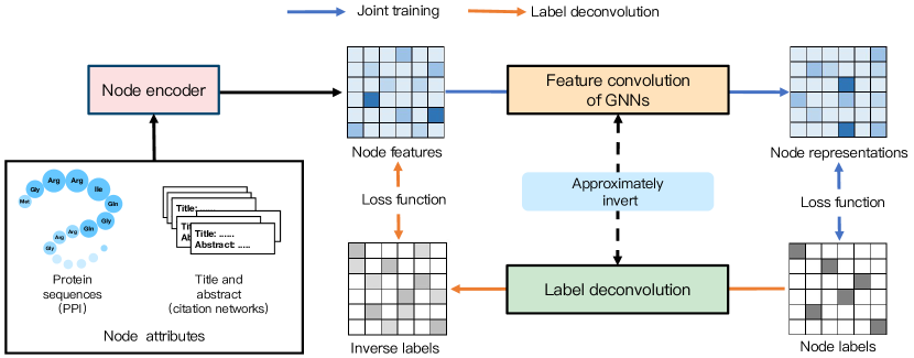
Figure 1: The idea of label deconvolution is to recover GNNs in the training phase of large node encoders (e.g. ESM2 [14] for protein sequences and Bert [15, 16] for texts), alleviating the learning bias from that by the joint training.

To address this challenge, we propose an efficient and effective label regularization technique, namely Label Deconvolution (LD), to alleviate the learning bias by integrating GNNs with NEs in the training phase of NEs. As shown by Fig. 1, given the true node labels for GNNs used in the joint training, LD aims to find equivalent labels for NEs (denoted by inverse labels) based on an approximate inverse mapping of GNNs. The inverse mapping guarantees that if we fit the output of NEs (denoted by node features) to the inverse labels, then the corresponding output of GNNs (denoted by node representations) is fitted to the true node labels. More importantly, we show that LD converges to the optimal objective function values by the joint training under some mild assumptions. To efficiently approximate the inverse mapping of GNNs, LD first decouples the memory and time-consuming feature convolution from GNNs inspired by [17, 18, 19]. By noticing that the node labels are fixed during training, LD pre-processes the memory and time-consuming inverse mapping of the feature convolution only once based on the fixed node labels, unlike the joint training, which performs the feature convolution at each training step to encode the learnable node features from NEs. Extensive experiments demonstrate LD significantly outperforms state-of-the-art methods by a significant margin on Open Graph Benchmark datasets.

2 Preliminaries

We introduce the problem setting in Section 2.1. Then, we introduce the joint training methods based on graph sampling in Section 2.2. Finally, we introduce the separate training methods in Section 2.3.

2.1 Node Representation Learning on Large-scale Attributed Graphs

We focus on node representation learning on a graph $\mathcal{G}=(\mathcal{V},\mathcal{E})$ with rich and useful node attributes $\{\mathbf{x}_{i}\}_{i=1}^{|\mathcal{V}|}$, where $\mathcal{V}$ is the set of all nodes and $\mathcal{E}$ is the set of all edges. As the true node attributes $\{\mathbf{x}_{i}\}_{i=1}^{|\mathcal{V}|}$ usually are high-dimensional texts, images, or protein sequences, a commonly-seen solution is to first extract $d_{f}$-dimensional node features $\{\mathbf{f}_{i}\}_{i=1}^{|\mathcal{V}|}$ from them as follows

$$\mathbf{f}_{i}^{(\beta)}=f(\mathbf{x}_{i};\beta)\in\mathbb{R}^{d_{f}},\,i=1,2,\dots,|\mathcal{V}|,$$ (1)

where $\beta$ represents the parameters of the node encoders (NEs). Empirically, large pre-trained models (e.g. ESM2 [14] for protein sequences and Bert [15, 16] for texts) serve as NEs $f$ due to their powerful ability to extract features [7, 8].

To further encode graph structures, graph neural networks take both nodes features $\mathbf{F}^{(\beta)}\in\mathbb{R}^{|\mathcal{V}|\times d_{f}}$ and adjacent matrix $\mathbf{A}\in\mathbb{R}^{|\mathcal{V}|\times|\mathcal{V}|}$ as inputs as follows

$$\mathbf{H}=\textsc{GNN}(\mathbf{F}^{(\beta)};\mathbf{A},\theta)\in\mathbb{R}^{|\mathcal{V}|\times d},$$ (2)

where $\mathbf{F}_{i,:}^{(\beta)}=\mathbf{f}_{i}^{(\beta)}$ denotes the $i$-th row of $\mathbf{F}^{(\beta)}$ and $\theta$ represents the parameters of the graph neural network. $\mathbf{A}_{ij}=1$ if $(i,j)\in\mathcal{E}$ and otherwise $\mathbf{A}_{ij}=0$. Then, GNNs output node representation $\mathbf{H}$.

For simplicity, we define the following notations. Given a set of nodes $\mathcal{B}$, let $\mathbf{M}_{\mathcal{B},:}=(\mathbf{M}_{i,:})_{i\in\mathcal{B}}$ denote the matrix consisting of $\mathbf{M}_{i,:}$ with all $i\in\mathcal{B}$, where $\mathbf{M}_{i,:}$ is the $i$-th row of $\mathbf{M}$. Given a vector function $f:\mathbb{R}^{d_{1}}\rightarrow\mathbb{R}^{d_{2}}$, we overload $\mathbf{M}^{\prime}=f(\mathbf{M})$ to denote a matrix function with ${\mathbf{M}}_{i,:}^{\prime}=f({\mathbf{M}}_{i,:})$.

2.2 Scalable Graph Neural Networks

Many scalable graph neural networks are categorized into two ideas in terms of data sampling and model architectures, respectively.

Graph Sampling for GNNs.  Equation (2) takes all node features as inputs and hence it is not scalable. To compute node representations in a mini-batch $\mathcal{B}$ of nodes, a commonly-seen solution is to sample a subgraph constructed by $\mathcal{B}$ as follows,

$$\mathbf{H}_{\mathcal{B},:} =\textsc{GNN}(\mathbf{F}_{G(\mathcal{B}),:};\mathbf{A}_{G(\mathcal{B})},\theta)\in\mathbb{R}^{|\mathcal{B}|\times d};$$ (3)

$$\mathbf{F}_{G(\mathcal{B}),:},\mathbf{A}_{G(\mathcal{B})} =\textsc{SAMPLER}(\mathbf{F},\mathbf{A}),$$ (4)

where $|\mathcal{B}|<<|G(\mathcal{B})|<<|\mathcal{V}|$. Notably, $|G(\mathcal{B})|$ used in existing graph sampling methods is significantly larger than the size of the mini-batch used in pre-trained NEs. If we further decrease the size of $|\mathcal{B}|$ or $|G(\mathcal{B})|$ in existing graph sampling methods to align their batch sizes, their performance will significantly drop, as shown in Table I. In experiments, the max batch size of pre-trained NEs is at most 12 (see Table VII), which is significantly smaller than $|G(\mathcal{B})|$. Therefore, the joint training of both NEs and GNNs by graph sampling is unaffordable.

TABLE I: Prediction performance with different sizes of sampled subgraph used in our experiments. We directly infer node features by the pre-trained models without fine-tuning. For GAS [20], we increase the number of subgraph partitions to decrease $|G(\mathcal{B})|$. For SAGE [21], we first decrease the number of target nodes $|\mathcal{B}|$ and then decrease the sampled neighbors to decrease $|G(\mathcal{B})|$.

GCN+GAS [20]	$|\mathcal{B}|$	84,260	25,574	2,566	264
	$|G(\mathcal{B})|$	96,536	48,871	4,691	3,958
	ACC	74.28%	74.14%	74.07%	67.46%
GAT+SAGE [21]	$|\mathcal{B}|$	8,662	866	87	87
	$|G(\mathcal{B})|$	131,381	131,119	130,948	80,529
	AUC	89.06%	88.74%	84.40%	81.27%

Decoupling Feature Convolution from GNNs as a Pre-processing Step.  To avoid the memory and time-consuming feature convolution of GNNs, other scalable GNNs (e.g. GAMLP [18] and SAGN [22]) first decouple the feature convolution from GNNs. Then, they pre-process the memory and time-consuming feature convolution only once based on fixed node features. However, as the node features are learnable by NEs, the idea is still unaffordable for the joint training of NEs and GNNs.

2.3 Existing Separate Training Frameworks

Given node labels $\mathbf{Y}$, the optimization problem is $\min_{\theta,\beta}\mathcal{L}(\textsc{GNN}(\mathbf{F}^{(\beta)},\mathbf{A};\theta),\mathbf{Y})$. To avoid severe scalability issue of feature convolutions, existing separate training frameworks propose to alternately optimize $\theta$ and $\beta$ by

$$\min_{\theta}\mathcal{L}(\textsc{GNN}(\mathbf{F}^{(\beta)};\mathbf{A},\theta),\mathbf{Y}),$$ (5)

and

$$\min_{\beta}\mathcal{L}^{\prime}(\mathbf{F}^{(\beta)},\mathbf{Y},\mathbf{A})\approx\min_{\beta}\mathcal{L}(\textsc{GNN}(\mathbf{F}^{(\beta)};\mathbf{A},\theta),\mathbf{Y}),$$ (6)

where $\mathcal{L}$ is the loss function for the true objective function and $\mathcal{L}^{\prime}$ is an approximation to $\mathcal{L}$.

Training Phase of GNNs (Optimize $\theta$).  In Equation (5), as the parameters of NEs $\beta$ are fixed, the scalable GNNs in Section 2.2 are applicable without the reduction of graph sizes based on the fixed node features $\mathbf{F}^{(\beta)}$.

Training Phase of NEs (Optimize $\beta$).  On the right side of Equation (6), the neighbor explosion issue remains unchanged as shown in Equation (3). Thus, existing separate training frameworks ignore feature convolutions in GNNs to design a new loss function $\mathcal{L}^{\prime}$, such as a self-supervision loss $\mathcal{L}_{ssl}(\mathbf{F}^{(\beta)},\mathbf{A})$ [7] or a supervision loss $\mathcal{L}(\psi(\mathbf{F}^{(\beta)}),\mathbf{Y})$ [8] with a scalable linear layer $\psi:\mathbb{R}^{d_{f}}\rightarrow\mathbb{R}^{d}$.

Notably, the training phase of NEs (i.e., the left side of Equation (6)) does not involve the parameters of GNNs $\theta$ in the formulation. Our formulation is different from GLEM [8], as LD and GLEM are based on different motivations. Specifically, LD aims to recover GNN in Equation (6), while GLEM aims to improve the quality of the pseudo labels $\mathbf{Y}_{\mathcal{V}_{test},:}$ on the test nodes $\mathcal{V}_{test}$ for semi-supervised learning. Thus, we omit the improvement of $\mathbf{Y}$ and assume that the node labels $\mathbf{Y}$ used in LD and GLEM are the same, as LD adopts the approach proposed by GLEM to improve the quality of the pseudo labels for semi-supervised learning.

3 Label Deconvolution

In this section, we propose a simple and efficient label regularization technique, namely Label Deconvolution (LD). Let node labels be $\mathbf{Y}$. If the task is semi-supervised (i.e., some node labels in graphs are missing), then we can first train GNNs based on the fixed node features inferred by pre-trained NEs.

LD is a separate training framework to train GNNs and NEs respectively. LD uses Equation (5) during the training phase of GNNs. During the training phase of NEs, we formulate the right side of Equation (6) as

$$\min_{\beta}\mathcal{L}(\mathbf{F}^{(\beta)},\hat{\mathbf{Y}});$$ (7)

$$\text{s.t.}\,\hat{\mathbf{Y}}=\textsc{GNN}^{-1}(\mathbf{Y};\mathbf{A},\theta)\,\text{(pre-processing)},$$ (8)

where $\textsc{GNN}^{-1}$ is the inverse mapping of GNN. We call $\hat{\mathbf{Y}}$ the inverse labels. As the parameters $\theta$ are fixed during the training phase of NEs, the key idea of LD is to pre-process $\hat{\mathbf{Y}}=\textsc{GNN}^{-1}(\mathbf{Y};\mathbf{A},\theta)$ to avoid executing the memory and time-consuming operation many times during training phase of NEs. Thus, the mini-batch version of Equation (7) is

$$\min_{\beta}\mathcal{L}(\mathbf{F}^{(\beta)}_{\mathcal{B},:},\hat{\mathbf{Y}}_{\mathcal{B},:}),$$

where $\mathcal{B}$ is the mini-batch of nodes.

As the inverse mapping of the non-linear GNN is difficult to compute exactly, we next derive an effective and efficient approximation to Equation (8). Specifically, we first introduce the spectral formulation of GNNs, which decouples linear feature convolutions from GNNs [17, 23]. Then, LD further avoids the inverse mapping of linear feature convolutions by parameterizing the inverse labels $\hat{\mathbf{Y}}$ with similar expressiveness.

3.1 Spectral-based GNNs

Many GNNs [24, 25, 23] are inspired by spectral filters, and thus the derivation of LD is based on the spectral-based GNNs [23], i.e.,

$$\mathbf{H}=\textsc{GNN}(\mathbf{F}^{(\beta)};\mathbf{A},\theta)=\phi(\hat{\mathbf{A}};\theta^{(\phi)})\psi(\mathbf{F}^{(\beta)};\theta^{(\psi)}),$$ (9)

where $\phi(\hat{\mathbf{A}};\theta^{(\phi)})=\sum_{i=0}^{N}\theta_{i}^{(\phi)}\hat{\mathbf{A}}^{i}$ is a polynomial spectral filter to perform linear feature convolutions, $\hat{\mathbf{A}}$ is the normalized adjacent matrix, and $\psi$ is a non-linear multi-layer perceptron. The weights $\theta^{(\phi)}$ are either learnable or fixed. The spectral-based GNN is powerful enough to produce arbitrary node predictions under some mild assumptions, as shown by [23]. Moreover, the assumptions hold on many real-world graphs. We elaborate on a connection between a wide range of GNNs (e.g., GCN [24], REVGAT [26], GAMLP [18], SAGN [22], and GAT [27] in the experiments) and the spectral-based GNN in Appendix A.

Thus, Equation (7) becomes

$$\min_{\beta,\theta}\mathcal{L}(\psi(\mathbf{F}^{(\beta)};\theta),\hat{\mathbf{Y}});$$ (10)

$$\text{s.t.}\,\hat{\mathbf{Y}}=\phi^{-1}(\hat{\mathbf{A}};\theta)\mathbf{Y}.\,\text{(pre-processing)}$$

Equation (10) preserves the scalable non-linear transformations of GNNs and pre-process the inverse of the graph diffusion matrix $\phi^{-1}(\hat{\mathbf{A}};\theta)$.

Notably, Equation (10) incorporates a part of the GNN parameters $\theta$ during the training phase of NEs. The incorporation significantly alleviates the learning bias from that by the joint training of NEs and GNNs, while it does not affect the scalability.

3.2 Label Deconvolution

To further avoid the inverse mapping of linear feature convolutions, we propose a trainable label deconvolution to generate the inverse labels $\mathbf{Y}^{(\gamma)}$. Label deconvolution aims to parameterize $\mathbf{Y}^{(\gamma)}$ with $\gamma$ such that the expressiveness of $\mathbf{Y}^{(\gamma)}$ is similar to $\phi^{-1}(\hat{\mathbf{A}};\theta)\mathbf{Y}$, i.e.,

$$\{\mathbf{Y}^{(\gamma)}:\gamma\}\approx\{\phi(\hat{\mathbf{A}};\theta)^{-1}\mathbf{Y}:\theta\}.$$

Thus, Equation (10) becomes

$$\min_{\beta,\theta,\gamma}\mathcal{L}(\psi(\mathbf{F}^{(\beta)};\theta),\mathbf{Y}^{(\gamma)}).$$ (11)

Comparing with Equation (10), Equation (11) implicitly incorporates parameters $\theta^{(\phi)}$ by our proposed reparameterization approach with $\gamma$. We provide the theoretical analysis in Section 4.

The key idea is inspired by the Cayley-Hamilton theorem. We first introduce two useful lemmas as follows.

Lemma 1.

[28, 29] Let the characteristic polynomial of a matrix $\mathbf{M}$ be $f(\lambda)=p_{n}\lambda^{n}+p_{n-1}\lambda^{n-1}+\cdots+p_{1}\lambda+p_{0}$. If the matrix $\mathbf{M}$ is invertible, then the inverse of $\mathbf{M}$ is

$$\mathbf{M}^{-1}=-\frac{1}{p_{0}}(p_{n}\mathbf{M}^{n-1}+p_{n-1}\mathbf{M}^{n-1}+\cdots+p_{2}\mathbf{M}+p_{1}\mathbf{I}).$$

Lemma 2.

[30, 29] The matrix $\mathbf{M}^{N}\in\mathbb{R}^{n\times n}$ can be expressed as a matrix polynomial of degree less than $n$, i.e.,

$$\mathbf{M}^{N}=\sum_{i=0}^{n-1}p_{i}\mathbf{M}^{i}.$$

The proposition follows immediately.

Proposition 1.

If $\phi(\hat{\mathbf{A}};\theta)^{-1}$ is invertible, then $\phi(\hat{\mathbf{A}};\theta)^{-1}$ is expressed as a linear combination of the matrix powers of $\hat{\mathbf{A}}$, i.e., $\phi(\hat{\mathbf{A}};\theta)^{-1}=\sum_{i=0}^{|\mathcal{V}|-1}\gamma_{i}\hat{\mathbf{A}}^{i}$.

Thus, we parameterize the inverse labels $\mathbf{Y}^{(\gamma)}$ by

$$\mathbf{Y}^{(\gamma)}=\sum_{i=0}^{N}\gamma_{i}\mathbf{K}_{i}=\sum_{i=0}^{N}\gamma_{i}\hat{\mathbf{A}}^{i}\mathbf{Y},$$ (12)

where $N$ is a hyper-parameter and the variables $\gamma_{i}\in\mathbb{R}$ are trainable parameters.

Intuitively, the $i$-hop labels $\mathbf{K}_{i}=\hat{\mathbf{A}}^{i}\mathbf{Y}$ are the (weighted) average of the labels in $k$-hop neighbors. For an $N$-layer GNN, the prediction (representation) of a node not only depends on its feature but also its $N$-hop neighbors’ features. Similarly, the feature of a node not only contributes to its prediction but also its $N$-hop neighbors’ predictions. Therefore, the $i$-hop labels are effective in alleviating the learning bias during the training phase of NEs.

The mini-batch version of Equation (12) is

$$\hat{\mathbf{Y}}_{\mathcal{B}}^{(\gamma)} =\sum_{i=0}^{N}\gamma_{i}[\mathbf{K}_{i}]_{\mathcal{B},:};$$ (13)

$$\mathbf{K}_{i} =(\hat{\mathbf{A}})^{i}\mathbf{Y}.\,\text{(pre-processing)}$$ (14)

where $\mathcal{B}$ is the mini-batch of nodes.

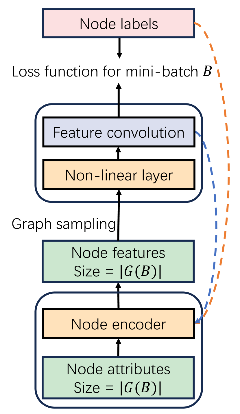
(a) Joint training.

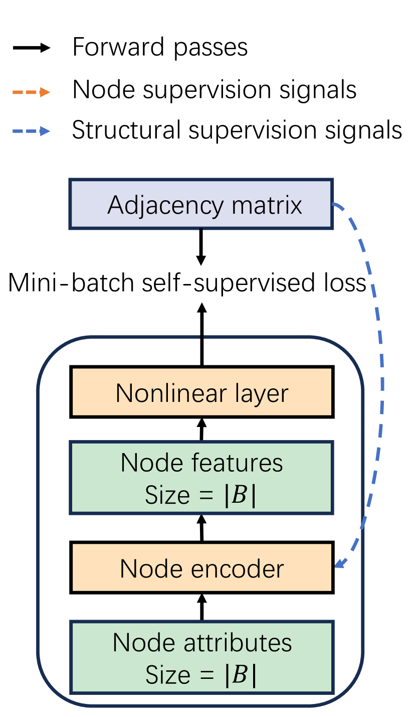
(b) GIANT.

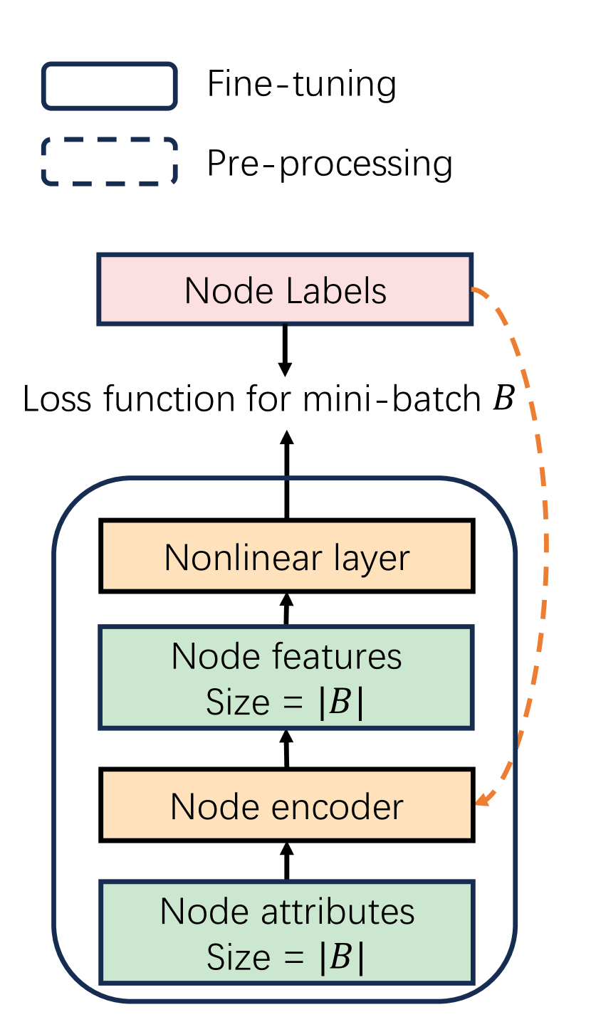
(c) GLEM.

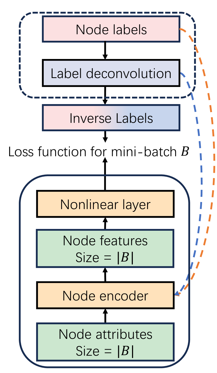
(d) Label deconvolution.

Figure 2: Comparison of different loss functions for NEs.

We summarize our algorithms in Algorithm 1. Given node labels be $\mathbf{Y}$, we first compute and save the $i$-hop labels $\mathbf{K}_{i}$ via Equation (14) during the pre-processing phase. During the training phase of NEs, we can efficiently compute the inverse labels $\mathbf{Y}^{(\gamma)}_{\mathcal{B}}$ and use them to train NEs and non-linear transformations $\psi$ of GNNs. Notably, we simultaneously optimize $\beta$, $\theta$, and $\gamma$ rather than alternately optimize. Finally, during the training phase of GNNs, we train scalable GNNs via Equation (5).

Algorithm 1 Label Deconvolution

1:  Input: Graph $\mathbf{A}$, attributes $\{\mathbf{x}_{i}\}$, (psuedo) labels $\mathbf{Y}$.

2:  Output: Node encoder with parameters $\beta$ and GNN with parameters $\theta$.

3:  // Pre-processing Phase:

4:  Compute $\mathbf{K}_{i}$ via Equation (14).

5:  // Training Phase of NEs (Optimize $\beta,\theta$):

6:  for $k=1,\dots,K_{1}$ do

7:     Randomly sample $\mathcal{B}$ from $\mathcal{V}$

8:     Compute the node features $\mathbf{F}^{(\beta)}_{\mathcal{B}}$ via Equation (1).

9:     Compute the inverse labels $\mathbf{Y}^{(\gamma)}_{\mathcal{B}}$ via Equation (13).

10:     Optimize $\beta,\theta,\gamma$ via the loss $\mathcal{L}(\psi(\mathbf{F}^{(\beta)}_{\mathcal{B}};\theta),\mathbf{Y}^{(\gamma)}_{\mathcal{B}})$

11:  end for

12:  Infer the node features $\mathbf{F}^{(\beta)}$ across all nodes.

13:  // Training Phase of GNNs (Optimize $\theta$ with fixed $\beta$):

14:  for $k=1,\dots,K_{2}$ do

15:     Compute the node features $\mathbf{H}_{\mathcal{B}}$ via Equation (3)

16:     Optimize $\theta$ via the loss $\mathcal{L}(\mathbf{H}_{\mathcal{B}},\mathbf{Y}_{\mathcal{B}})$

17:  end for

3.3 Comparision with Different Loss Functions for NEs

As shown in Section 2.3, many existing separate training frameworks propose various loss functions to approximate the right side of Equation (6), leading to a significant learning bias from that by the joint training, which directly optimizes $\min_{\theta,\beta}\mathcal{L}(\textsc{GNN}(\mathbf{F}^{(\beta)},\mathbf{A};\theta),\mathbf{Y})$. We summarize the learning bias in terms of node labels and graph structures. Fig. 2 shows the loss functions of the joint training, LD, GIANT [7], and GLEM [8]. LD integrates the graph structures with the node labels to generate the inverse labels, maintaining a similar learning behavior to that of the joint training. However, GIANT and GLEM neglect either the graph structures or the node labels, leading to a significant learning bias.

Although LD and the joint training share a similar learning learning behavior, LD is more memory-efficient than the joint training. Specifically, to compute the loss on a mini-batch of nodes $\mathcal{B}$, the NEs of LD encode the attributes in the mini-batch $\mathcal{B}$ with the memory complexity $\mathcal{O}(|\mathcal{B}|)$. However, the NEs of the joint training encode the attributes in a sampled subgraph with size $G(\mathcal{B})$, leading to larger memory complexity $\mathcal{O}(|G(\mathcal{B})|)$ than LD.

Table II shows the complexity of different training methods during the training phase of NEs and the supervision signals for NEs. LD and GLEM are the fastest and most memory-efficient algorithms among all methods. More importantly, LD incorporates graph structures $\mathbf{A}$ into the supervision signals for NEs, compared with GLEM.

TABLE II: Computational complexity of different training methods during the training phase of NEs and the supervision signals for NEs. $\|\mathbf{A}\|_{0}$ is the number of edges and satisfies $|\mathcal{V}|\leq\|\mathbf{A}\|_{0}\leq|\mathcal{V}|^{2}$.

Methods	Time	Memory	Supervision
	Complexity	Complexity	Signals for NEs
Joint training	$\mathcal{O}(|\mathcal{V}|\frac{|G(\mathcal{B})|}{|\mathcal{B}|})$	$\mathcal{O}(|G(\mathcal{B})|)$	$\mathbf{Y}$ & $\mathbf{A}$
GIANT [7]	$\mathcal{O}(\|\mathbf{A}\|_{0})$	$\mathcal{O}(|\mathcal{B}|)$	$\mathbf{A}$
GLEM [8]	$\mathcal{O}(|\mathcal{V}|)$	$\mathcal{O}(|\mathcal{B}|)$	$\mathbf{Y}$
LD	$\mathcal{O}(|\mathcal{V}|)$	$\mathcal{O}(|\mathcal{B}|)$	$\mathbf{Y}$ & $\mathbf{A}$

4 Theoretical Results

In this section, we analyze the learning behaviors of LD. Specifically, we show that LD converges to the optimal objective function values by the joint training under some mild assumption, while GLEM—one of the state-of-the-art separate training frameworks—may converge to the sub-optimal objective function values. We provide detailed proofs of the theorems in Appendix B.

We formulate the training process of LD as

$$\min_{\theta,\beta_{LD}}\,\mathcal{L}(\textsc{GNN}(\mathbf{F}^{(\beta_{LD})},\mathbf{A};\theta),\mathbf{Y});$$

$$\text{s.t.}\,\beta_{LD}\in\arg\min_{\beta}\min_{\gamma,\theta}\mathcal{L}(\psi(\mathbf{F}^{(\beta)};\theta),\mathbf{Y}^{(\gamma)}).$$

Similarly, the training process of GLEM is

$$\min_{\theta,\beta_{GLEM}}\,\mathcal{L}(\textsc{GNN}(\mathbf{F}^{(\beta_{GLEM})},\mathbf{A};\theta),\mathbf{Y});$$

$$\text{s.t.}\,\beta_{GLEM}\in\arg\min_{\beta}\min_{\theta}\mathcal{L}(\psi(\mathbf{F}^{(\beta)};\theta),\mathbf{Y}).$$

For simplicity, the loss function $\mathcal{L}$ is a mean squared loss.

TABLE III: Statistics of the datasets in the experiments.

#Dataset	#Node attributes	#Graphs	#Metric	Total #Nodes	Total #Edges	#Avg. Degree
ogbn-arxiv	Textural titles and abstracts	1	Accuracy	169,343	1,157,799	6.8
ogbn-product	Textural descriptions for products	1	Accuracy	2,449,029	61,859,076	25.3
ogbn-protein	Protein sequences	1	ROC-AUC	132,534	39,561,252	298.5

4.1 Motivating Example

Consider a graph $\mathcal{G}=(\mathcal{V},\mathcal{E})=(\{(1,2,3,4)\},\{(1,2),(2,1),(3,4),(4,3)\})$ with one-hot node attributes $\mathbf{X}=(\mathbf{e}_{1},\mathbf{e}_{2},\mathbf{e}_{2},\mathbf{e}_{3})^{\top}$. The $i$-th element of $\mathbf{e}_{i}\in\mathbb{R}^{3}$ is zero and the others are zero. The corresponding node labels are one-hot vectors $\mathbf{Y}=(\mathbf{e}_{2},\mathbf{e}_{1},\mathbf{e}_{3},\mathbf{e}_{2})^{\top}$. Clearly, we have $\mathbf{Y}=\hat{\mathbf{A}}\mathbf{X}$. We use a GNN model $\textsc{GNN}(\mathbf{F},\mathbf{A})=\hat{\mathbf{A}}\mathbf{F}$ and a learnable node encoder $\mathbf{F}=\mathbf{X}\beta$ to fix $\mathbf{Y}$. Table IV shows the learned node features $\mathbf{F}$ and the accuracy of LD and GLEM. The node labels of nodes $1,4$ are incorrect for the node encoder such that $\mathbf{F}_{GLEM}$ can not distinguish them. Thus, the GNN model further can not distinguish nodes $1,4$ as they also share the same neighbor. In contrast, inverse labels help LD learn correct node features and further give the correct prediction. We provide the detailed derivation in Appendix B.2.

TABLE IV: The motivating example for LD and GLEM.

$\mathbf{Y}$	$\mathbf{X}$		$\mathbf{F}_{GLEM}$	$\mathbf{A}\mathbf{F}_{GLEM}$	$\mathbf{F}_{LD}$	$\mathbf{A}\mathbf{F}_{LD}$
$\mathbf{e}_{2}$	$\mathbf{e}_{1}$		$\mathbf{e}_{2}$	$(\mathbf{e}_{1}+\mathbf{e}_{3})/2$	$\mathbf{e}_{1}$	$\mathbf{e}_{2}$
$\mathbf{e}_{1}$	$\mathbf{e}_{2}$		$(\mathbf{e}_{1}+\mathbf{e}_{3})/2$	$\mathbf{e}_{2}$	$\mathbf{e}_{2}$	$\mathbf{e}_{1}$
$\mathbf{e}_{3}$	$\mathbf{e}_{2}$		$(\mathbf{e}_{1}+\mathbf{e}_{3})/2$	$\mathbf{e}_{2}$	$\mathbf{e}_{2}$	$\mathbf{e}_{3}$
$\mathbf{e}_{2}$	$\mathbf{e}_{3}$		$\mathbf{e}_{2}$	$(\mathbf{e}_{1}+\mathbf{e}_{3})/2$	$\mathbf{e}_{3}$	$\mathbf{e}_{2}$
Accuracy			-	0%	-	100%

4.2 Theory

Our theory is based on an observation that the node labels not only depend on node attributes but also graph structures. Thus, we use the following assumption.

Assumption 1.

The node labels $\mathbf{Y}$ are given by graph structures and node attributes, i.e., $\mathbf{Y}=\phi(\hat{\mathbf{A}})\psi(\mathbf{F}^{*})$, where $\hat{\mathbf{A}}=\mathbf{D}^{-1}\mathbf{A}$ is the normalized adjacent matrix, $\mathbf{D}$ is the degree matrix, and $\mathbf{F}^{*}_{:,i}=f(\mathbf{x}_{i})$ represents the node feature extracted from the attribute $\mathbf{a}_{i}$. Let $\psi:\mathbb{R}^{d_{f}}\rightarrow\mathbb{R}^{d}$ be an unknown encoder like multi-layer perceptrons (MLPs) and $\phi(\hat{\mathbf{A}})=\sum_{n=0}^{N}\alpha_{n}^{*}\hat{\mathbf{A}}^{n}$ be an unknown polynomial graph signal filter. We assume that $\phi(\hat{\mathbf{A}})$ is invertible.

We parameterize GNN by a spectral-based GNN [23], i.e.,

$$\textsc{GNN}(\mathbf{F}^{(\beta)},\mathbf{A};\theta)=\phi(\hat{\mathbf{A}};\theta)\psi(\mathbf{F}^{(\beta)};\theta).$$

Recent works theoretically show that the expressiveness of the spectral-based GNN is equal to the 1-WL test—which bounds the expressiveness of many GNNs [23]. Clearly, the joint training of NEs and GNNs converges to the optimal objective function values, i.e.

$$\min_{\theta,\beta}\,\mathcal{L}(\textsc{GNN}(\mathbf{F}^{(\beta)},\mathbf{A};\theta),\mathbf{Y})=0.$$

We show $\min_{\theta}\,\mathcal{L}(\textsc{GNN}(\mathbf{F}^{(\beta_{LD})},\mathbf{A};\theta),\mathbf{Y})=0$ by the following theorem.

Theorem 1.

If Assumption 1 holds, then there exists $\beta_{LD}\in\arg\min_{\beta}\min_{\gamma,\theta}\mathcal{L}(\psi(\mathbf{F}^{(\beta)};\theta),\mathbf{Y}^{(\gamma)})$ such that $\min_{\theta}\,\mathcal{L}(\textsc{GNN}(\mathbf{F}^{(\beta_{LD})},\mathbf{A};\theta),\mathbf{Y})=0$.

Notably, the motivating example in Section 4.1 is a counterexample for $\beta_{GLEM}$. Specifically, in the motivating example, we have $\min_{\theta}\,\mathcal{L}(\textsc{GNN}(\mathbf{F}^{(\beta_{GLEM})},\mathbf{A};\theta),\mathbf{Y})>0$ for all $\beta_{GLEM}\in\arg\min_{\beta}\min_{\theta}\mathcal{L}(\psi(\mathbf{F}^{(\beta)};\theta),\hat{\mathbf{Y}})$.

5 Experiments

In this section, we compare LD with the state-of-the-art training methods for node classification on multiple large-scale attributed graphs, including citation networks, co-purchase networks, and protein–protein association networks. We run all experiments five times on a single NVIDIA GeForce RTX 3090 (24 GB).

5.1 Experimental Setups

5.1.1 Datasets

We conduct experiments on ogbn-arxiv, ogbn-product, and ogbn-protein from widely-used Open Graph Benchmark (OGB) [13], whose graphs are citation networks, co-purchase networks, and protein–protein association networks respectively. OGB provides an official leaderboard for a fair comparison of different methods. They are large-scale (up to 2.4M nodes and 61.9M edges in our experiments) and have been widely used in previous works [20]. We follow the realistic train/validation/test splitting methods of OGB, such as by time (ogbn-arxiv), by sales ranking (ogbn-product), and by species which the proteins come from (ogbn-protein). Their statistics are shown in Table III.

5.1.2 Node Attributes

For ogbn-arxiv and ogbn-product, we use titles/abstracts and textual descriptions for products provided by OGB [13] as node attributes. For ogbn-protein, we map the protein identifiers into the protein sequences based on the STRING database [5].

5.1.3 Prediction Tasks and Evaluation Metric

We use the official evaluation metric provided by OGB [13]. Specifically, we use accuracy as the evaluation metric for ogbn-arxiv and ogbn-product, which aim to predict the primary categories of the arxiv papers and the categories of products respectively in a multi-class classification setup. We use ROC-AUC as the evaluation metric for ogbn-protein, which aims to predict the presence of protein functions in a multi-label binary classification setup.

5.1.4 Node Encoders and GNN architectures

For each dataset, we use the state-of-the-art GNN architectures on the OGB leaderboards, including GCN [24], REVGAT [26], GAMLP [18], SAGN [22], and GAT [27]. For the textual attributes in ogbn-arxiv, following [8], we use DeBERTa [16] as the node encoder. For ogbn-product, we follow [8] to integrate GAMLP with DeBERTa [16], and follow [7] to integrate SAGN with Bert [15]. For the protein sequences in ogbn-protein, we use ESM2 [14] as the node encoder.

TABLE V: Performance of node classification (mean ± std%). We bold the best result and underline the second best result.

Datasets	GNNs		$\mathbf{X}_{\text{OGB}}$	$\mathbf{X}_{\text{GIANT}}$	$\mathbf{X}_{\text{PNE}}$	$\mathbf{X}_{\text{FNE}}$	$\mathbf{X}_{\text{GLEM}}$	$\mathbf{X}_{\text{LD}}$
ogbn-arxiv	GCN	val	73.00 ± 0.17	74.89 ± 0.17	74.74 ± 0.11	76.39 ± 0.11	76.86 ± 0.19	76.84 ± 0.09
		test	71.74 ± 0.29	73.29 ± 0.10	74.04 ± 0.16	75.90 ± 0.16	75.93 ± 0.19	76.22 ± 0.10
	REVGAT	val	75.01 ± 0.10	77.01 ± 0.09	75.36 ± 0.18	75.99 ± 0.18	77.49 ± 0.17	77.62 ± 0.08
		test	74.02 ± 0.18	75.90 ± 0.19	75.14 ± 0.08	75.52 ± 0.08	76.97 ± 0.19	77.26 ± 0.17
ogbn-product	GAMLP	val	93.12 ± 0.03	93.99 ± 0.04	93.21 ± 0.05	93.19 ± 0.05	94.19 ± 0.01	94.15 ± 0.03
		test	83.54 ± 0.09	83.16 ± 0.07	84.51 ± 0.05	82.88 ± 0.05	85.09 ± 0.21	86.45 ± 0.12
	SAGN	val	93.02 ± 0.04	93.64 ± 0.05	93.25 ± 0.04	93.84 ± 0.06	-	93.99 ± 0.02
		test	84.35 ± 0.09	86.67 ± 0.09	85.37 ± 0.08	84.81 ± 0.07	-	87.18 ± 0.04
ogbn-protein	GAT	val	93.75 ± 0.19	-	95.16 ± 0.06	95.05 ± 0.12	-	95.27 ± 0.07
		test	88.09 ± 0.16	-	88.94 ± 0.14	88.66 ± 0.08	-	89.42 ± 0.07

5.1.5 Baselines

As shown in Section 2.3, many existing methods first extract node features $\mathbf{F}^{(\beta)}$ based on different approximations to Equation (6) and then train GNNs based on the same Equation (5). The node features of our baselines include (1) the features provided by OGB [13], denoted as $\mathbf{X}_{\text{OGB}}$; (2) the embeddings inferred by pre-trained NEs, denoted as $\mathbf{X}_{\text{PNE}}$; (3) the LM embeddings inferred by fine-tuned NEs with the true node labels, denoted as $\mathbf{X}_{\text{FNE}}$; (4) the GIANT features [7], denoted as $\mathbf{X}_{\text{GIANT}}$; (5) the GLEM features [8], denoted as $\mathbf{X}_{\text{GLEM}}$. We do not include the joint training as a baseline due to the scalability issues introduced in Section 2.2. We summarize the key differences between the baselines and LD in Table VI.

TABLE VI: The key differences between the baselines and LD.

Features	Pre-trained	Training with	Training with
	models	(pseudo) labels	graph structures
$\mathbf{X}_{\text{OGB}}$	$\times$	$\times$	$\times$
$\mathbf{X}_{\text{PNE}}$	$\checkmark$	$\times$	$\times$
$\mathbf{X}_{\text{FNE}}$	$\checkmark$	$\checkmark$	$\times$
$\mathbf{X}_{\text{GIANT}}$	$\checkmark$	$\times$	$\checkmark$
$\mathbf{X}_{\text{GLEM}}$	$\checkmark$	$\checkmark$	$\times$
$\mathbf{X}_{\text{LD}}$	$\checkmark$	$\checkmark$	$\checkmark$

5.1.6 Implementation Details of LD

We implement the inverse labels $\mathbf{Y}^{(\gamma)}$ to ensure the label constraints for the multi-class classification and multi-label binary classification setup. Specifically, we parameterize $\gamma=\textsc{SOFTMAX}(\gamma^{\prime})$ with a uniform initialization to ensure that the inverse labels are positive and they have a similar norm to the true labels, i.e., $\mathbf{Y}^{(\gamma)}_{ij}\geq 0$ and $\|\mathbf{Y}^{(\gamma)}\|\approx\|\mathbf{Y}\|$. We implement the loss function

$$\mathcal{L}(\mathbf{H},\mathbf{Y}^{(\gamma)})=l(\mathbf{H},(1-\alpha)\mathbf{Y}+\alpha\textsc{NORMALIZE}(\mathbf{Y}^{(\gamma)})),$$ (15)

where $l$ is the cross entropy loss and $\alpha$ is a hyper-parameter to avoid overfitting. For the multi-class classification, the normalization function $\textsc{NORMALIZE}(\mathbf{Y}^{(\gamma)})_{ij}=\mathbf{Y}^{(\gamma)}_{ij}/(\sum_{k}\mathbf{Y}^{(\gamma)}_{ik})$ ensures that the output is a probability distribution. For the multi-label binary classification setup, the normalization function clamps all elements in $\mathbf{Y}^{(\gamma)}$ into the range $[0,1]$.

We use the PyTorch library [31] to implement label deconvolution. To ensure a fair comparison, the hyperparameters for pre-retrained NEs and GNNs in experiments are the same as GLEM [8]. We follow the implementation of the top-ranked GNNs in the OGB leaderboard. LD introduces two hyper-parameters $N$ and $\alpha$ defined in Equations (12) and (15) respectively. We set $N$ to be the number of convolutional layers used in GNNs in experiments. We set $\alpha=1$ for the GNN models which use the fixed normalized adjacent matrix to aggregate messages from neighbors (e.g., GCN, GAMLP, and SAGN). We search best $\alpha$ in $\{0.2,0.5,1.0\}$ for REVGAT and GAT which use the attention-based aggregation, as we approximate the graph attention by the normalized adjacent matrix inspired by [32] (see Appendix A for detailed derivation).

For the semi-supervised node classification, we first generate pseudo labels of the nodes in the valid and test sets following GLEM [8]. To this end, we train GNNs based on $\mathbf{X}_{\text{PNE}}$. We do not follow the EM algorithm of GLEM [8] to iteratively update pseudo labels, as the EM-iteration does not significantly improve performance but suffers from expensive training costs.

5.2 Overall performance

We report the overall performance of LD and baselines in Table V. Overall, LD outperforms all baselines on the three datasets with different GNN backbones. As GLEM and GIANT mainly focus on the text-attributed graph, they do not provide the results on the ogbn-protein dataset, whose node attributes are protein sequences. The official implementation of GLEM on ogbn-products with SAGN performs much worse than the reported accuracy of 0.8736 on the test data. Therefore, we omit this result in Table V.

By noticing that $\mathbf{X}_{\text{FNE}}$ outperforms $\mathbf{X}_{\text{PNE}}$ except for ogbn-arxiv, directly fine-tuning with the true labels may limit the final performance. The phenomenon verifies the motivating example in Table IV and Assumption 1, i.e., node labels depend on not only node attributes but also graph structures. Specifically, in ogbn-product, many stores may use product descriptions to attract customers rather than introduce the products, and thus difficult to reflect the product categories. In ogbn-protein, the edges represent biologically meaningful associations between proteins [13] and are important for protein functions. In ogbn-arxiv, although the abstract and introduction of a scientific paper almost reflect the subject areas of the paper, $\mathbf{X}_{\text{LD}}$ still outperforms $\mathbf{X}_{\text{FNE}}$. The pseudo-labels introduced by GLEM are difficult to overcome this issue, as the pseudo-labels aim to approximate the true labels. Finally, GIANT aims to introduce graph structure information to node features by self-supervised learning, while it may incorporate much task-irrelevant information due to the neglect of node labels.

5.3 Runtime

Another appealing feature of LD is that it is significantly faster than GLEM—the state-of-the-art separate training method—as shown in Table VII. First, LD significantly outperforms FLM—which fine-tuned NEs with the true labels—in terms of accuracy, although LD is slightly slower than FLM. To improve the accuracy of FLM, GLEM integrates pseudos labels with the true labels by an iterative knowledge-distilling process, which requires fine-tuning pre-trained NEs and inferring the whole dataset many times, leading to expensive costs. In contrast, LD only fine-tunes pre-trained NEs once and infers node features twice as shown in Algorithm 1, leading to significantly cheap costs. Specifically, on the ogbn-product dataset, the accuracy of LD is 1.36% higher than GLEM, and the runtime is less than one-third of GLEM.

TABLE VII: The runtime of different separate training methods. Bold font indicates the best result and underlining indicates the second best result. We evaluate the max batch size of LM (max bsz.) and training time on a single 24GB GPU.

Datasets	Metric	FNE	GLEM	LD
ogbn-arxiv	accuracy	75.52	75.93	76.22
	max bsz.	12	12	12
	time/epoch	3150s	4131s	4360s
	time/total	2.52h	6.53h	3.02h
ogbn-product	accuracy	82.88	85.09	86.45
	max bsz.	12	12	12
	time/epoch	8880s	13133s	12871s
	time/total	16.88h	75.67h	24.78h
ogbn-protein	accuracy	88.66	-	89.42
	max bsz.	4	-	4
	time/epoch	8931s	-	12696s
	time/total	17.73h	-	36.22h

5.4 Contribution of LD

Compared with FNE, LD additionally uses pseudo labels on the valid and test data. Thus, we conduct the ablation study in Table VIII to show the effectiveness of the inverse labels based on the true labels and the pseudo labels. We introduce $\mathbf{X}_{\text{WO/LD}}$, which fine-tunes pre-trained models with the true labels on train data and the pseudo labels on valid and test data. We set $\alpha=0$ in Equation (15) to implement $\mathbf{X}_{\text{WO/LD}}$. Other hyper-parameters and training pipelines are the same as that of $\mathbf{X}_{\text{LD}}$. As shown in Table VIII, the pseudo labels also improve the prediction performance against $\mathbf{X}_{\text{FNE}}$ based on the true labels, and $\mathbf{X}_{\text{LD}}$ significantly improves the prediction performance on all datasets against $\mathbf{X}_{\text{WO/LD}}$. Specifically, on the ogbn-product dataset, $\mathbf{X}_{\text{WO/LD}}$ is approximately 0.95% higher than $\mathbf{X}_{\text{FNE}}$, while $\mathbf{X}_{\text{LD}}$ is significantly 2.62% higher than $\mathbf{X}_{\text{WO/LD}}$.

TABLE VIII: Results of ablation study.

Datasets	GNNs	$\mathbf{X}_{\text{FNE}}$	$\mathbf{X}_{\text{WO/LD}}$	$\mathbf{X}_{\text{LD}}$
ogbn-arxiv	REVGAT	75.52±0.08	75.35±0.12	77.26±0.17
ogbn-product	GAMLP	82.88±0.05	83.83±0.18	86.45±0.12
ogbn-protein	GAT	88.66±0.08	89.15±0.12	89.42±0.07

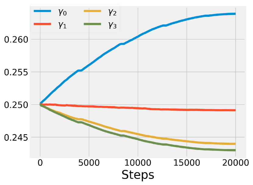
(a) REVGAT & ogbn-arxiv

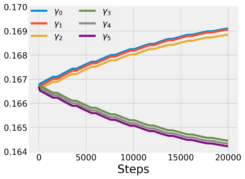
(b) GAMLP & ogbn-product

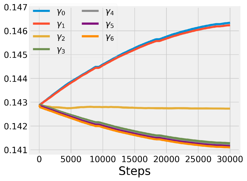
(c) GAT & ogbn-protein

Figure 3: Training curves of weights $\gamma_{i}$.

(a) Text similarity

(b) Label similarity of the inverse labels

(c) Label similarity of the true labels

Figure 4: Text similarity and label similarity.

(a) REVGAT & ogbn-arxiv

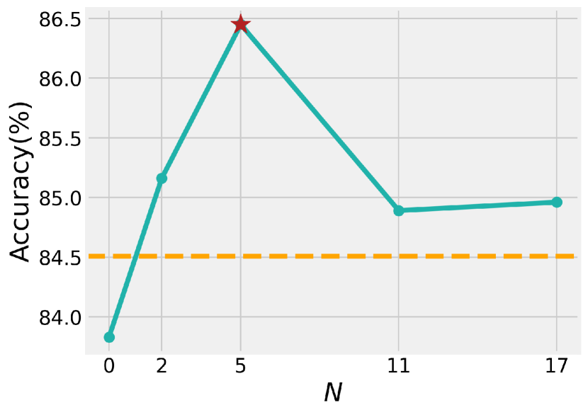
(b) GAMLP & ogbn-product

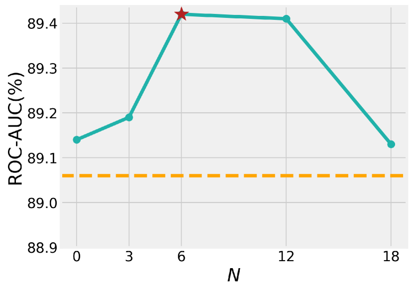
(c) GAT & ogbn-protein

Figure 5: The performance of node classification under varying values of label convolution layers $N$. The used GNN layers are 3, 5, and 6 on the ogbn-arxiv, ogbn-product, and ogbn-protein, respectively.

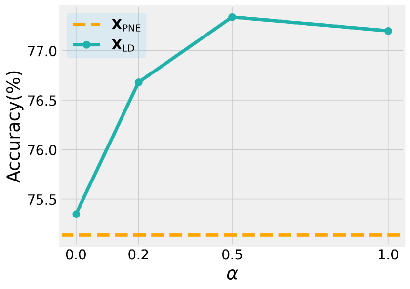
(a) REVGAT & ogbn-arxiv

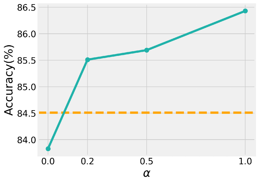
(b) GAMLP & ogbn-product

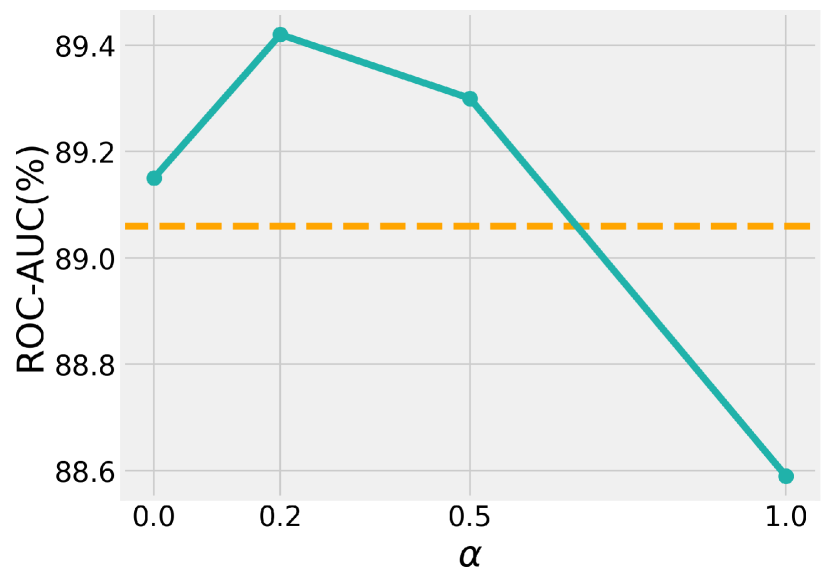
(c) GAT & ogbn-protein

Figure 6: The performance of node classification under varying values of $\alpha$.

5.5 Analysis of Inverse Labels

In this section, we empirically compare the difference between the inverse labels and the true labels.

From Equation (12), the inverse labels $\mathbf{Y}^{(\gamma)}$ are a weighted sum of the true labels and their $i$-hops neighbors’ labels. We thus plot the weights $\gamma_{i}$ during the fine-tuning process in Fig. 3. The inverse labels tend to be the true labels or the $i$-hops neighbors’ labels with small $i$. This is because the true labels and the $i$-hops neighbors’ labels with small $i$ are still the most important supervision signals among all hops’ labels for node classification. Moreover, the $i$-hops neighbors’ labels with large $i$ suffer from the over-smoothing issue, i.e., the $i$-hops neighbors’ labels may tend to be indistinguishable as $i$ increases [33]. Notably, the weight $\gamma_{i}$ does not converge to a trivial solution where $\gamma_{0}\rightarrow 1,\gamma_{i}\rightarrow 0,i\geq 1$. This implies that other hops’ labels are helpful to node feature extraction and label deconvolution effectively alleviates the label noise from the graph structures.

In order to further compare the inverse labels and the true labels, we show the similarity of the node attributes and the similarity of labels in Fig. 4. We randomly selected several pairs of nodes from the ogbn-arxiv dataset with highly similar texts (i.e., the text similarity is more than 0.6) but different labels (nodes 0 and 1, 2 and 3, 4 and 5). Following [7], we use the TF-IDF algorithm and the cosine similarity to evaluate the text similarity and the label similarity, respectively. Fig. 4(a) each pair of nodes has high similarity, but the nodes in different pairs have low similarity as we select them independently. Fig.s 4(b) and 4(c) show that the inverse labels provide similar supervision signals for the nodes with similar texts and different supervision signals for the nodes with different texts. However, the true labels fail. Therefore, the inverse labels preserve the true attribute semantics by reducing label noise in the graph structures.

5.6 Hyper-parameter Sensitivity

The additional hyper-parameters of LD contain $N$ and $\alpha$ defined in Equations (12) and (15) respectively. We provide the performance curves on different datasets for $N$ and $\alpha$. When exploring the effect of a hyper-parameter, we fix the other as their best values.

As shown in Fig. 5, LD achieves the best performance when $N$ is equal to the number of convolution layers of GNNs on the ogbn-product and ogbn-protein datasets. On the ogbn-arxiv dataset, the performance at $N=6$ is slightly better than that at $N=3$, which is the number of the convolution layers of GNNs. Indeed, $N$ highly impacts the expressiveness of label deconvolution. The inverse labels under large $N$ increase the expressiveness while may suffer from overfitting.

As shown in Fig. 6, LD achieves the best performance with large $\alpha$ on the ogbn-arxiv and ogbn-product datasets. Moreover, the performance of LD with $\alpha=1$ is similar to the best performance on these datasets. LD with the large $\alpha$ indicates that the inverse labels dominate the training behavior of NEs. However, on the ogbn-arxiv dataset, LD achieves the best performance with a small $\alpha=0.2$. As the average degree of ogbn-protein is significantly larger than ogbn-arxiv and ogbn-product (see Tab. III), the $i$-hop labels $\mathbf{K}_{i}=\hat{\mathbf{A}}^{i}\mathbf{Y}$ under the large degree are easily become indistinguishable, leading to the over-smoothing issue [33]. Despite the over-smoothing issue, LD with $\alpha=0.2$ still outperforms LD with $\alpha=0.0$, which only uses the true labels. Overall, the inverse labels of LD significantly improve the prediction performance.

6 related work

In this section, we discuss some works related to our proposed method.

6.1 Training Methods for large NEs and GNNs

An ideal idea is to jointly train large NEs and GNNs to simultaneously optimize their parameters. However, due to the severe scalability issue of GNNs [21, 34, 35] and the excessive model complexity of pre-trained models, the joint training often runs out of the GPU memory. To avoid the out-of-memory issue, some methods [9, 10] restrict the feature convolutions to very small sampled subgraphs, severely hurting topological structures in graphs.

To encode graph structures and node attributes, many studies propose to separately train NEs and GNNs. For example, some methods [7, 36] first propose scalable self-supervised learning to train NEs—which encode node attributes into node features—and then integrate node features with graph structures by GNNs. The proposed self-supervised tasks aim to incorporate graph topological information into node features. However, it is unclear whether the additional graph topological information is helpful to GNNs, which encode similar information. Besides, GLEM [8] proposes an iterative pseudo-label distillation framework, which iteratively trains NEs and GNNs. The pseudo-label distillation framework aims to improve the quality of the pseudo labels, which is orthogonal to our proposed LD.

Notably, many existing training methods mainly focus on the text-attributed graph (TAG) [37] whose node attributes are texts. An appealing feature of LD is that it is applicable to general node attributes including protein sequences.

6.2 Scalable Graph Neural Networks

To avoid full-batch inference and training on the large-scale graphs, the graph sampling techniques run GNNs on sample small subgraphs. We follow [38] to categorize these methods into node, layer, and subgraph-wise sampling. Node-wise sampling methods [21, 39, 40] recursively sample a fixed number of neighbors to construct different subgraphs for different GNN layers. Although they decrease the bases in the exponentially increasing sizes of the subgraph with the number of GNN layers, they still suffer from the neighbor explosion issue. To tackle this issue, layer-wise sampling methods [41, 42, 43] use importance sampling to recursively sample different subgraphs with the same size for different GNN layers. However, they suffer from sparse connections between sampled nodes, leading unstable training process. To improve stability and accelerate convergence, subgraph-wise sampling methods [4, 35, 20, 34] sample the same subgraph with more connections for different GNN layers. Despite their success, reducing the subgraph sizes significantly sacrifices the model performance. In practice, they are usually applicable to shallow GNNs with large subgraph sizes rather than deep pre-trained node encoders and GNNs with very small subgraph sizes [8].

Another line of related work is to design scalable GNNs by moving feature convolutions into the pre-processing process [17, 19, 44, 18, 23]. They first perform feature convolutions for the initial node features and save them as additional node features in the pre-processing process. Then, we design various node classifiers to learn node representations without message passing. JacobiConv [23] shows that the expressiveness of the pre-convolution architectures is the same as 1-WL under some mild assumptions for node classification. However, the pre-processing scheme is not applicable to the learned node features by node encoders. Label deconvolution is a novel and effective pre-processing scheme to extract node features and hence it fills this gap.

7 conclusion

In this paper, we propose an efficient and effective label regularization technique, namely Label Deconvolution (LD), to alleviate the learning bias from that by the joint training. we show that LD converges to the optimal objective function values by the joint training under some mild assumption Extensive experiments on Open Graph Benchmark datasets demonstrate that LD significantly outperforms state-of-the-art training methods in terms of prediction performance and efficiency.

Appendix A Linear feature convolution and Non-linear Transformation in GNNs

In this section, we introduce linear feature convolution and non-linear transformation in GNNs including GCN, REVGAT, GAMLP, SAGN, and GAT. Let the set of $\{1,2,\dots,p\}$ be $[p]$.

Many GNNs [24, 25, 27, 18, 26] iteratively update node representations in two stages: linear feature convolution and non-linear transformation

$$\mathbf{H}^{(i+1/2)} =\phi^{(i+1)}(\mathbf{A};\theta)\mathbf{H}^{(i)};\,\text{(linear feature convolution)}$$ (16)

$$\mathbf{H}^{(i+1)} =\psi^{(i+1)}(\mathbf{H}^{(i+1/2)};\theta),\,\text{(non-linear transformation)}$$ (17)

where $\phi^{(i+1)}(\mathbf{A};\theta)\in\mathbb{R}^{|\mathcal{V}|\times|\mathcal{V}|}$ is the diffusion matrix constructed from the adjacent matrix $\mathbf{A}$. An $N$-layer GNN iteratively takes node features $\mathbf{H}^{(0)}=\mathbf{F}^{(\beta)}$ as input and outputs node representations $\mathbf{H}=\mathbf{H}^{(N)}$ at the $N$-th layer, i.e.,

$$\mathbf{H}=\psi^{(N)}\circ\phi^{(N)}\circ\psi^{(N-1)}\circ\phi^{(N-1)}\cdots\phi^{(1)}(\mathbf{F}^{(\beta)}).$$

The notorious neighbor explosion issue is due to the linear feature convolutions $\phi^{(i)}$ rather than the non-linear transformations. Thus, we decouple the inverse of all linear feature convolutions by changing the order of these operations as follows

$$\mathbf{H} \approx(\phi^{(N)}\circ\phi^{(N-1)}\cdots\phi^{(1)})(\psi^{(N)}\circ\psi^{(N-1)}\cdots\psi^{(1)})(\mathbf{F}^{(\beta)})$$

$$=\phi(\mathbf{A};\theta)\psi(\mathbf{F}^{(\beta)};\theta),$$ (18)

where $\phi(\mathbf{A};\theta)=\prod_{i=1}^{n}\phi^{(i)}(\mathbf{A};\theta)\in\mathbb{R}^{|\mathcal{V}|\times|\mathcal{V}|}$ is still a diffusion matrix and $\psi=\psi^{(N)}\circ\psi^{(N-1)}\circ\cdots\psi^{(1)}$ is a non-linear multi-layer perceptron.

GCN [24].  GCN iteratively updates node representations by

$$\mathbf{H}^{(i+1)}=\sigma(\hat{\mathbf{A}}\mathbf{H}^{(i)}\mathbf{W}^{(i+1)}),$$

where $\mathbf{W}^{(i+1)}$ is the trainable weights of the $(i+1)$-th layer and $\sigma$ is an activation function (e.g. ReLU, TanH, and Sigmoid). $\hat{\mathbf{A}}=\mathbf{D}^{-1}\mathbf{A}$ is the normalized adjacent matrix, where $\mathbf{D}$ is the degree matrix with $\mathbf{D}_{i,i}=\sum_{j}\mathbf{A}_{i,j}$ and $\mathbf{D}_{i,j}=0,\forall i\neq j$. By letting $\mathbf{H}^{(i+1/2)}=\hat{\mathbf{A}}\mathbf{H}^{(i)}$, the corresponding linear feature convolution and non-linear transformation are

$$\mathbf{H}^{(i+1/2)} =\phi^{(i+1)}(\mathbf{A};\theta)\mathbf{H}^{(i)}=\hat{\mathbf{A}}\mathbf{H}^{(i)},$$

$$\mathbf{H}^{(i+1)} =\psi^{(i+1)}(\mathbf{H}^{(i+1/2)};\mathbf{W}^{(l+1)})=\sigma(\mathbf{H}^{(i+1/2)}\mathbf{W}^{(i+1)})$$

respectively. Thus, the resulting diffusion matrix and the multi-layer perceptron are

$$\phi(\mathbf{A};\theta) =\hat{\mathbf{A}}^{N},$$

$$\psi(\mathbf{X};\mathbf{W}^{(i)},i=1,2,\dots,N) =\sigma(\cdots\sigma(\mathbf{X}\mathbf{W}^{(1)})\cdots\mathbf{W}^{(N)}).$$

REVGAT [26].  At the $(i+1)$-th layer, REVGAT first partition $\mathbf{H}^{(i)}$ into $C$ groups $(\mathbf{H}^{(i)}_{1},\mathbf{H}^{(i)}_{2},\dots,\mathbf{H}^{(i)}_{C})$ and then update node representations in each group by

$$\overline{\mathbf{H}}^{(i+1)}_{0} =\sum_{j=2}^{C}\mathbf{H}^{(i)}_{j};$$

$$\overline{\mathbf{H}}^{(i+1)}_{j} =\textsc{GAT}^{(i+1)}_{j-1}+\mathbf{H}^{(i)}_{j},\,j\in[C],$$

$$\textsc{GAT}^{(i+1)}_{j-1} =\sigma(\mathbf{A}(\overline{\mathbf{H}}^{(i+1)}_{j-1},\theta)\overline{\mathbf{H}}^{(i+1)}_{j-1}\mathbf{W}^{(i+1)}_{j});$$

$$\mathbf{H}^{(i+1)} =\textsc{MLP}(\overline{\mathbf{H}}^{(i+1)});$$

where $\mathbf{A}(\mathbf{H}^{(i)},\theta)$ is a learnable attention matrix, $\mathbf{W}^{(i+1)}$ is the trainable weights of the $(i+1)$-th layer, and $\sigma$ is an activation function. As recent works show that we can replace the graph attention with a normalized random vector to achieve similar performance [32], we approximate $\mathbf{A}(\mathbf{H}^{(i)},\theta)$ by a fixed normalized adjacent matrix $\hat{\mathbf{A}}$. There exists $NC$ feature convolutions $\phi^{(i+1)}_{j}$ and non-linear transformation $\psi^{(i+1)}_{j}$. If $j=1$, by letting $\mathbf{H}^{(i+1)}_{1/2}=\hat{\mathbf{A}}\mathbf{H}^{(i+1)}$, the corresponding linear feature convolution is

$$\mathbf{H}^{(i+1)}_{1/2} =\phi^{(i+1)}_{1}(\mathbf{A};\theta)\overline{\mathbf{H}}^{(i+1)}=\hat{\mathbf{A}}\mathbf{H}^{(i+1)};$$

and the non-linear transformation $\psi^{(i+1)}_{1}$ is

$$\overline{\mathbf{H}}^{(i+1)}_{1} =\textsc{GAT}^{(i+1)}_{0}+\mathbf{H}^{(i)}_{1},$$

$$\textsc{GAT}^{(i+1)}_{0} =\sigma(\sum_{j=2}^{C}[\mathbf{H}^{(i+1)}_{1/2}]_{j}\mathbf{W}^{(i+1)}_{1}).$$

If $j\in[2,C-1]$, by letting $\mathbf{H}^{(i+1)}_{j-1/2}=\hat{\mathbf{A}}\overline{\mathbf{H}}^{(i+1)}_{j-1}$, the corresponding linear feature convolution is

$$\mathbf{H}^{(i+1)}_{j-1/2} =\phi^{(i+1)}_{j}(\mathbf{A};\theta)\overline{\mathbf{H}}^{(i+1)}_{j-1}=\hat{\mathbf{A}}\overline{\mathbf{H}}^{(i+1)}_{j-1},$$

and the non-linear transformation $\psi^{(i+1)}_{j}$ compute $\overline{\mathbf{H}}^{(i+1)}_{j}$ by

$$\overline{\mathbf{H}}^{(i+1)}_{j} =\textsc{GAT}^{(i+1)}_{j-1}+\mathbf{H}^{(i)}_{j},$$

$$\textsc{GAT}^{(i+1)}_{j-1} =\sigma(\mathbf{H}^{(i+1)}_{j-1/2}\mathbf{W}^{(i+1)}_{j}).$$

If $j=C$, by letting $\mathbf{H}^{(i+1)}_{C-1/2}=\hat{\mathbf{A}}\overline{\mathbf{H}}^{(i+1)}_{C-1}$, the corresponding linear feature convolution is

$$\mathbf{H}^{(i+1)}_{C-1/2} =\phi^{(i+1)}_{C}(\mathbf{A};\theta)\overline{\mathbf{H}}^{(i+1)}_{C-1}=\hat{\mathbf{A}}\overline{\mathbf{H}}^{(i+1)}_{C-1},$$

and the non-linear transformation $\psi^{(i+1)}_{C}$ compute $\overline{\mathbf{H}}^{(i+1)}$ by

$$\overline{\mathbf{H}}^{(i+1)}_{C} =\textsc{GAT}^{(i+1)}_{C-1}+\mathbf{H}^{(i)}_{C},$$

$$\textsc{GAT}^{(i+1)}_{C-1} =\sigma(\mathbf{H}^{(i+1)}_{C-1/2}\mathbf{W}^{(i+1)}_{C})$$

$$\mathbf{H}^{(i+1)} =\textsc{MLP}(\overline{\mathbf{H}}^{(i+1)}).$$

Thus, the resulting diffusion matrix is

$$\phi(\mathbf{A};\theta) =\hat{\mathbf{A}}^{NC},$$

and the resulting $\psi$ is an $N$-layer reversible network

$$\overline{\mathbf{H}}^{(i+1)}_{0} =\sum_{j=2}^{C}\mathbf{H}^{(i)}_{j};$$

$$\overline{\mathbf{H}}^{(i+1)}_{j} =\sigma(\overline{\mathbf{H}}^{(i+1)}_{j-1}\mathbf{W}^{(i+1)}_{j})+\mathbf{H}^{(i)}_{j},\,j\in[C],$$

$$\mathbf{H}^{(i+1)} =\textsc{MLP}(\overline{\mathbf{H}}^{(i+1)}).$$

GAMLP [18].  Given the node features $\mathbf{X}$ and the label embeddings $\mathbf{H}_{Y}$, GAMLP learns node representations by

$$\mathbf{H} =\textsc{MLP}(\mathbf{H}_{X})+\beta\textsc{MLP}(\mathbf{H}_{Y});$$

$$\mathbf{H}_{X} =\sum_{i=0}^{N}\theta_{i}\hat{\mathbf{A}}^{i}\mathbf{X},$$

where MLP is a multi-layer perception, $\beta$ is a hyper-parameter, and $\theta_{i}$ is the learned weights (e.g., recursive attention and JK attention). As the computation costs of the label embeddings $\mathbf{H}_{Y}$ are very expensive during the training phase of NEs, we set $\beta=0$. We use $\theta_{i}\in\mathbb{R}$ in the derivation of this paper, as the scalar weight is powerful enough to produce arbitrary node predictions under some mild conditions[23]. Thus, GAMLP performs the linear feature convolution and the non-linear transformation only once by

$$\mathbf{H}^{(1/2)} =\phi^{(1)}(\mathbf{A};\theta)\mathbf{H}^{(0)}=(\sum_{i=0}^{N}\theta_{i}\hat{\mathbf{A}}^{i})\mathbf{H}^{(0)},$$

and

$$\mathbf{H}^{(1)} =\psi^{(1)}(\mathbf{H}^{(1/2)},)=\textsc{MLP}(\mathbf{H}^{(1/2)}).$$

Thus, $\phi$ and $\psi$ are

$$\phi(\mathbf{A};\theta) =\sum_{i=0}^{N}\theta_{i}\hat{\mathbf{A}}^{(i)},$$

$$\psi(\mathbf{X}) =\textsc{MLP}(X).$$

SAGN [22].  Given the node features $\mathbf{X}$, SAGN learns node representations by

$$\mathbf{Z} =\mathbf{X}||\hat{\mathbf{A}}\mathbf{X}||\hat{\mathbf{A}}^{2}\mathbf{X}||\dots\hat{\mathbf{A}}^{N}\mathbf{X};$$

$$\mathbf{H} =\textsc{MLP}(\mathbf{Z})=\sum_{i=0}^{N}\textsc{MLP}_{i}(\hat{\mathbf{A}}^{i}\mathbf{X}),$$

where $||$ denotes concatenation. As the nonlinearity of $\textsc{MLP}_{i}$ is unnecessary for SAGN to reach high expressiveness [23], we remove the nonlinearity of $\textsc{MLP}_{i}$ by

$$\mathbf{H} =\sum_{i=0}^{N}\textsc{MLP}_{i}(\hat{\mathbf{A}}^{i}\mathbf{X})\approx\sum_{i=0}^{N}\hat{\mathbf{A}}^{i}\mathbf{X}\theta_{i}.$$

We follow the derivation of GAMLP to approximate $\phi$ and $\psi$ by

$$\phi(\mathbf{A};\theta) =\sum_{i=0}^{N}\theta_{i}\hat{\mathbf{A}}^{(i)},$$

$$\psi(\mathbf{X}) =\textsc{MLP}_{0}(X).$$

We preserve the architecture $\textsc{MLP}_{0}$ of the true SAGN to alleviate the learning bias.

GAT [27].  GAT iteratively updates node representations by

$$\mathbf{H}^{(i+1)}=\sigma(\textsc{MLP}(\mathbf{A}(\mathbf{H}^{(i)},\mathcal{E},\theta)\mathbf{H}^{(i)}\mathbf{W}^{(i+1)})),$$

where $\mathbf{A}(\mathbf{H}^{(i)},\mathcal{E},\theta)$ is a learnable attention matrix, $\mathcal{E}$ denotes the edge features, MLP is a multi-layer perception introduced by NGNN [45], $\mathbf{W}^{(i+1)}$ is the trainable weights of the $(i+1)$-th layer, and $\sigma$ is an activation function (e.g. ReLU, TanH, and Sigmoid). As recent works show that we can replace the graph attention with a normalized random vector to achieve similar performance [32], we approximate $\mathbf{A}(\mathbf{H}^{(i)},\mathcal{E},\theta)$ by a fixed normalized adjacent matrix $\hat{\mathbf{A}}$. By letting $\mathbf{H}^{(i+1/2)}=\hat{\mathbf{A}}\mathbf{H}^{(i)}$, the corresponding linear feature convolution and non-linear transformation are

$$\mathbf{H}^{(i+1/2)} =\phi^{(i+1)}(\mathbf{A};\theta)\mathbf{H}^{(i)}=\hat{\mathbf{A}}\mathbf{H}^{(i)},$$

$$\mathbf{H}^{(i+1)} =\psi^{(i+1)}(\mathbf{H}^{(i+1/2)};\mathbf{W}^{(i+1)})$$

$$=\sigma(\textsc{MLP}(\mathbf{H}^{(i+1/2)}\mathbf{W}^{(i+1)}))$$

respectively. Thus, the resulting diffusion matrix and the multi-layer perceptron are

$$\phi(\mathbf{A};\theta) =\hat{\mathbf{A}}^{N},$$

$$\psi(\mathbf{X}) =\sigma(\textsc{MLP}(\cdots\sigma(\textsc{MLP}(\mathbf{X}\mathbf{W}^{(1)}))\cdots\mathbf{W}^{(N)})).$$

Appendix B Detailed proofs

B.1 Proof of Proposition 1

It follows from Lemma 1 that $\phi(\mathbf{A};\theta)^{-1}$ is expressed as a linear combination of the matrix powers of $\hat{\mathbf{A}}$, i.e.,

$$\phi(\mathbf{A};\theta)^{-1} =\sum_{j=0}^{|\mathcal{V}|-1}p_{j}\phi(\mathbf{A};\theta)^{j}$$

$$=\sum_{j=0}^{|\mathcal{V}|-1}p_{j}(\sum_{i=0}^{N}\theta_{i}^{(\phi)}\hat{\mathbf{A}}^{i})^{j}$$

$$=\sum_{i=0}^{N(|\mathcal{V}|-1)}q_{i}\hat{\mathbf{A}}^{i}.$$

It follows from Lemma 2 that there exists $\gamma_{i}$ such that

$$\phi(\mathbf{A};\theta)^{-1}=\sum_{i=0}^{|\mathcal{V}|-1}\gamma_{i}\hat{\mathbf{A}}^{i}.$$

B.2 Solution to the motivating example in Section 4.1

The node attributes, the node labels, and the normalized adjacent matrix are $\mathbf{X}=(\mathbf{e}_{1},\mathbf{e}_{2},\mathbf{e}_{2},\mathbf{e}_{3})^{\top}=\begin{bmatrix}1&0&0\\ 0&1&0\\ 0&1&0\\ 0&0&1\end{bmatrix}$, $\mathbf{Y}=(\mathbf{e}_{2},\mathbf{e}_{1},\mathbf{e}_{3},\mathbf{e}_{2})^{\top}=\begin{bmatrix}0&1&0\\ 1&0&0\\ 0&0&1\\ 0&1&0\end{bmatrix}$, and $\hat{\mathbf{A}}=\begin{bmatrix}0&1&0&0\\ 1&0&0&0\\ 0&0&0&1\\ 0&0&1&0\end{bmatrix}.$

GLEM first solve

$$\beta_{GLEM}=\arg\min_{\beta}\|\mathbf{X}\beta-\mathbf{Y}\|_{F}^{2}=\begin{bmatrix}0&1&0\\ 0.5&0&0.5\\ 0&1&0\end{bmatrix}.$$

Then, the final prediction of GLEM is

$$\mathbf{A}\mathbf{F}_{GLEM}=\mathbf{A}\mathbf{X}\beta_{GLEM}=\begin{bmatrix}0.5&0&0.5\\ 0&1&0\\ 0&1&0\\ 0.5&0&0.5\end{bmatrix}=\mathbf{Y}.$$

LD first solve

$$\beta_{LD},\gamma_{0}^{*},\gamma_{1}^{*} =\arg\min_{\beta,\gamma_{0},\gamma_{1}}\|\gamma_{0}\mathbf{X}\beta+\gamma_{1}\mathbf{A}\mathbf{X}\beta-\mathbf{Y}\|_{F}^{2}$$

$$=\begin{bmatrix}1&0&0\\ 0&1&0\\ 0&0&1\end{bmatrix},0,1.$$

Then, the final prediction of LD is

$$\mathbf{A}\mathbf{F}_{LD}=\mathbf{A}\mathbf{X}\beta_{LD}=\begin{bmatrix}0&1&0\\ 1&0&0\\ 0&0&1\\ 0&1&0\end{bmatrix}.$$

B.3 Proof of Theorem 1

Proof.

We first show that $\min_{\beta,\theta,\gamma}\mathcal{L}(\psi(\mathbf{F}^{(\beta)};\theta),\mathbf{Y}^{(\gamma)})=0$. Let $\phi(\hat{\mathbf{A}},\theta^{*})=\phi(\mathbf{A})$, $\psi(\mathbf{F}^{*},\theta^{*})=\psi(\mathbf{F}^{*})$, and $\mathbf{F}^{\beta^{*}}=\mathbf{F}^{*}$, where $\phi(\mathbf{A})$, $\psi(\mathbf{F}^{*})$, and $\mathbf{F}^{*}$ are defined in Assumption 1. Then, we have $\phi(\hat{\mathbf{A}},\theta^{*})=\phi(\mathbf{A})$ is invertible, we have

$$\mathcal{L}(\psi(\mathbf{F}^{(\beta^{*})};\theta^{*}),\phi(\hat{\mathbf{A}};\theta^{*})^{-1}\mathbf{Y})=0.$$

It follows from Lemmas 1 and 2 that $\phi(\mathbf{A};\theta)^{-1}$ is expressed as a linear combination of the matrix powers of $\hat{\mathbf{A}}$, i.e., $\phi(\mathbf{A};\theta)^{-1}=\sum_{i=0}^{|\mathcal{V}|-1}\gamma_{i}^{*}\hat{\mathbf{A}}^{i}$. Therefore, we have $\min_{\beta,\theta,\gamma}\mathcal{L}(\psi(\mathbf{F}^{(\beta)};\theta),\mathbf{Y}^{(\gamma)})=\mathcal{L}(\psi(\mathbf{F}^{(\beta^{*})};\theta^{*}),\hat{\mathbf{Y}}^{(\gamma^{*})})=0$.

Let $\beta_{LD}=\beta^{*}$. Then, we have

$$\min_{\theta}\,\mathcal{L}(\textsc{GNN}(\mathbf{F}^{(\beta_{LD})},\mathbf{A};\theta),\mathbf{Y})$$

$$= \mathcal{L}(\phi(\hat{\mathbf{A}};\theta^{*})\psi(\mathbf{F}^{(\beta_{LD})};\theta^{*}),\mathbf{Y})=0.$$

∎

References

- [1] K. Wang, Z. Shen, C. Huang, C.-H. Wu, Y. Dong, and A. Kanakia, “Microsoft Academic Graph: When experts are not enough,” Quantitative Science Studies, vol. 1, no. 1, pp. 396–413, 02 2020. [Online]. Available: https://doi.org/10.1162/qss_a_00021
- [2] J. Tang, J. Zhang, L. Yao, J. Li, L. Zhang, and Z. Su, “Arnetminer: Extraction and mining of academic social networks,” in KDD’08, 2008, pp. 990–998.
- [3] J. Yang and J. Leskovec, “Defining and evaluating network communities based on ground-truth,” Knowledge and Information Systems, vol. 42, no. 1, pp. 181–213, 2015.
- [4] W.-L. Chiang, X. Liu, S. Si, Y. Li, S. Bengio, and C.-J. Hsieh, “Cluster-gcn: An efficient algorithm for training deep and large graph convolutional networks,” in Proceedings of the 25th ACM SIGKDD International Conference on Knowledge Discovery & Data Mining, 2019, pp. 257–266.
- [5] D. Szklarczyk, R. Kirsch, M. Koutrouli, K. Nastou, F. Mehryary, R. Hachilif, A. L. Gable, T. Fang, N. T. Doncheva, S. Pyysalo, P. Bork, L. J. Jensen, and C. von Mering, “The STRING database in 2023: protein-protein association networks and functional enrichment analyses for any sequenced genome of interest,” Nucleic Acids Res, vol. 51, no. D1, pp. D638–D646, Jan 2023.
- [6] T. G. O. Consortium, “The gene ontology resource: 20 years and still going strong,” Nucleic Acids Research, vol. 47, pp. D330 – D338, 2018. [Online]. Available: https://api.semanticscholar.org/CorpusID:53222305
- [7] E. Chien, W.-C. Chang, C.-J. Hsieh, H.-F. Yu, J. Zhang, O. Milenkovic, and I. S. Dhillon, “Node feature extraction by self-supervised multi-scale neighborhood prediction,” in International Conference on Learning Representations, 2022. [Online]. Available: https://openreview.net/forum?id=KJggliHbs8
- [8] J. Zhao, M. Qu, C. Li, H. Yan, Q. Liu, R. Li, X. Xie, and J. Tang, “Learning on large-scale text-attributed graphs via variational inference,” in The Eleventh International Conference on Learning Representations, 2023. [Online]. Available: https://openreview.net/forum?id=q0nmYciuuZN
- [9] J. Zhu, Y. Cui, Y. Liu, H. Sun, X. Li, M. Pelger, T. Yang, L. Zhang, R. Zhang, and H. Zhao, “Textgnn: Improving text encoder via graph neural network in sponsored search,” in Proceedings of the Web Conference 2021, ser. WWW ’21. New York, NY, USA: Association for Computing Machinery, 2021, p. 2848–2857. [Online]. Available: https://doi.org/10.1145/3442381.3449842
- [10] L. Huang, D. Ma, S. Li, X. Zhang, and H. Wang, “Text level graph neural network for text classification,” in Proceedings of the 2019 Conference on Empirical Methods in Natural Language Processing and the 9th International Joint Conference on Natural Language Processing (EMNLP-IJCNLP). Hong Kong, China: Association for Computational Linguistics, Nov. 2019, pp. 3444–3450. [Online]. Available: https://aclanthology.org/D19-1345
- [11] J. Gilmer, S. S. Schoenholz, P. F. Riley, O. Vinyals, and G. E. Dahl, “Neural message passing for quantum chemistry,” in Proceedings of the 34th International Conference on Machine Learning, ser. Proceedings of Machine Learning Research, D. Precup and Y. W. Teh, Eds., vol. 70. PMLR, 06–11 Aug 2017, pp. 1263–1272. [Online]. Available: https://proceedings.mlr.press/v70/gilmer17a.html
- [12] W. L. Hamilton, “Graph representation learning,” Synthesis Lectures on Artificial Intelligence and Machine Learning, vol. 14, no. 3, pp. 1–159, 2020.
- [13] W. Hu, M. Fey, M. Zitnik, Y. Dong, H. Ren, B. Liu, M. Catasta, and J. Leskovec, “Open graph benchmark: Datasets for machine learning on graphs,” in Advances in Neural Information Processing Systems, 2020, pp. 22 118–22 133.
- [14] Z. Lin, H. Akin, R. Rao, B. Hie, Z. Zhu, W. Lu, N. Smetanin, A. dos Santos Costa, M. Fazel-Zarandi, T. Sercu, S. Candido et al., “Language models of protein sequences at the scale of evolution enable accurate structure prediction,” bioRxiv, 2022.
- [15] J. Devlin, M.-W. Chang, K. Lee, and K. Toutanova, “BERT: Pre-training of deep bidirectional transformers for language understanding,” in Proceedings of the 2019 Conference of the North American Chapter of the Association for Computational Linguistics: Human Language Technologies, Volume 1 (Long and Short Papers). Minneapolis, Minnesota: Association for Computational Linguistics, Jun. 2019, pp. 4171–4186. [Online]. Available: https://aclanthology.org/N19-1423
- [16] P. He, X. Liu, J. Gao, and W. Chen, “Deberta: Decoding-enhanced bert with disentangled attention,” in International Conference on Learning Representations, 2021. [Online]. Available: https://openreview.net/forum?id=XPZIaotutsD
- [17] F. Wu, A. Souza, T. Zhang, C. Fifty, T. Yu, and K. Weinberger, “Simplifying graph convolutional networks,” in Proceedings of the 36th International Conference on Machine Learning, ser. Proceedings of Machine Learning Research, K. Chaudhuri and R. Salakhutdinov, Eds., vol. 97. PMLR, 09–15 Jun 2019, pp. 6861–6871. [Online]. Available: https://proceedings.mlr.press/v97/wu19e.html
- [18] W. Zhang, Z. Yin, Z. Sheng, Y. Li, W. Ouyang, X. Li, Y. Tao, Z. Yang, and B. Cui, “Graph attention multi-layer perceptron,” in Proceedings of the 28th ACM SIGKDD Conference on Knowledge Discovery and Data Mining, ser. KDD ’22. New York, NY, USA: Association for Computing Machinery, 2022, p. 4560–4570. [Online]. Available: https://doi.org/10.1145/3534678.3539121
- [19] H. Zhu and P. Koniusz, “Simple spectral graph convolution,” in International Conference on Learning Representations, 2021. [Online]. Available: https://openreview.net/forum?id=CYO5T-YjWZV
- [20] M. Fey, J. E. Lenssen, F. Weichert, and J. Leskovec, “Gnnautoscale: Scalable and expressive graph neural networks via historical embeddings,” in Proceedings of the 38th International Conference on Machine Learning, ser. Proceedings of Machine Learning Research, M. Meila and T. Zhang, Eds., vol. 139. PMLR, 18–24 Jul 2021, pp. 3294–3304. [Online]. Available: https://proceedings.mlr.press/v139/fey21a.html
- [21] W. Hamilton, Z. Ying, and J. Leskovec, “Inductive representation learning on large graphs,” in Advances in Neural Information Processing Systems, 2017, p. 1025–1035.
- [22] C. Sun, H. Gu, and J. Hu, “Scalable and adaptive graph neural networks with self-label-enhanced training,” arXiv preprint arXiv:2104.09376, 2021.
- [23] X. Wang and M. Zhang, “How powerful are spectral graph neural networks,” in Proceedings of the 39th International Conference on Machine Learning, ser. Proceedings of Machine Learning Research, K. Chaudhuri, S. Jegelka, L. Song, C. Szepesvari, G. Niu, and S. Sabato, Eds., vol. 162. PMLR, 17–23 Jul 2022, pp. 23 341–23 362. [Online]. Available: https://proceedings.mlr.press/v162/wang22am.html
- [24] T. N. Kipf and M. Welling, “Semi-supervised classification with graph convolutional networks,” in ICLR (Poster). OpenReview.net, 2017.
- [25] M. Chen, Z. Wei, Z. Huang, B. Ding, and Y. Li, “Simple and deep graph convolutional networks,” in Proceedings of the 37th International Conference on Machine Learning, ser. Proceedings of Machine Learning Research, H. D. III and A. Singh, Eds., vol. 119. PMLR, 13–18 Jul 2020, pp. 1725–1735. [Online]. Available: http://proceedings.mlr.press/v119/chen20v.html
- [26] G. Li, M. Müller, B. Ghanem, and V. Koltun, “Training graph neural networks with 1000 layers,” in Proceedings of the 38th International Conference on Machine Learning, ser. Proceedings of Machine Learning Research, M. Meila and T. Zhang, Eds., vol. 139. PMLR, 18–24 Jul 2021, pp. 6437–6449. [Online]. Available: https://proceedings.mlr.press/v139/li21o.html
- [27] P. Veličković, G. Cucurull, A. Casanova, A. Romero, P. Liò, and Y. Bengio, “Graph Attention Networks,” in International Conference on Learning Representations, 2018.
- [28] H. P. Decell, Jr., “An application of the cayley-hamilton theorem to generalized matrix inversion,” SIAM Review, vol. 7, no. 4, pp. 526–528, 1965. [Online]. Available: https://doi.org/10.1137/1007108
- [29] X.-D. Zhang, Eigenanalysis. Cambridge University Press, 2017, p. 413–510.
- [30] A. Forsgren, “Inertia-controlling factorizations for optimization algorithms,” Applied Numerical Mathematics, vol. 43, no. 1, pp. 91–107, 2002, 19th Dundee Biennial Conference on Numerical Analysis. [Online]. Available: https://www.sciencedirect.com/science/article/pii/S0168927402001198
- [31] A. Paszke, S. Gross, F. Massa, A. Lerer, J. Bradbury, G. Chanan, T. Killeen, Z. Lin, N. Gimelshein, L. Antiga, A. Desmaison, A. Kopf, E. Yang, Z. DeVito, M. Raison, A. Tejani, S. Chilamkurthy, B. Steiner, L. Fang, J. Bai, and S. Chintala, “Pytorch: An imperative style, high-performance deep learning library,” in Advances in Neural Information Processing Systems 32, 2019, pp. 8024–8035.
- [32] X. Li and Y. Cheng, “Irregular message passing networks,” Know.-Based Syst., vol. 257, no. C, dec 2022. [Online]. Available: https://doi.org/10.1016/j.knosys.2022.109919
- [33] Q. Li, Z. Han, and X.-M. Wu, “Deeper insights into graph convolutional networks for semi-supervised learning,” in Proceedings of the AAAI conference on artificial intelligence, vol. 32, no. 1, 2018.
- [34] Z. Shi, X. Liang, and J. Wang, “LMC: Fast training of GNNs via subgraph sampling with provable convergence,” in International Conference on Learning Representations, 2023. [Online]. Available: https://openreview.net/forum?id=5VBBA91N6n
- [35] H. Zeng, H. Zhou, A. Srivastava, R. Kannan, and V. Prasanna, “Graphsaint: Graph sampling based inductive learning method,” in International Conference on Learning Representations, 2020. [Online]. Available: https://openreview.net/forum?id=BJe8pkHFwS
- [36] M. Yasunaga, J. Leskovec, and P. Liang, “Linkbert: Pretraining language models with document links,” in Association for Computational Linguistics (ACL), 2022.
- [37] J. Yang, Z. Liu, S. Xiao, C. Li, D. Lian, S. Agrawal, A. Singh, G. Sun, and X. Xie, “Graphformers: Gnn-nested transformers for representation learning on textual graph,” in Advances in Neural Information Processing Systems, M. Ranzato, A. Beygelzimer, Y. Dauphin, P. Liang, and J. W. Vaughan, Eds., vol. 34. Curran Associates, Inc., 2021, pp. 28 798–28 810. [Online]. Available: https://proceedings.neurips.cc/paper_files/paper/2021/file/f18a6d1cde4b205199de8729a6637b42-Paper.pdf
- [38] Y. Ma and J. Tang, Deep Learning on Graphs. Cambridge University Press, 2021.
- [39] J. Chen, J. Zhu, and L. Song, “Stochastic training of graph convolutional networks with variance reduction,” in Proceedings of the 35th International Conference on Machine Learning, ser. Proceedings of Machine Learning Research, J. Dy and A. Krause, Eds., vol. 80. PMLR, 10–15 Jul 2018, pp. 942–950.
- [40] H. Yu, L. Wang, B. Wang, M. Liu, T. Yang, and S. Ji, “GraphFM: Improving large-scale GNN training via feature momentum,” in Proceedings of the 39th International Conference on Machine Learning, ser. Proceedings of Machine Learning Research, K. Chaudhuri, S. Jegelka, L. Song, C. Szepesvari, G. Niu, and S. Sabato, Eds., vol. 162. PMLR, 17–23 Jul 2022, pp. 25 684–25 701. [Online]. Available: https://proceedings.mlr.press/v162/yu22g.html
- [41] J. Chen, T. Ma, and C. Xiao, “FastGCN: Fast learning with graph convolutional networks via importance sampling,” in International Conference on Learning Representations, 2018. [Online]. Available: https://openreview.net/forum?id=rytstxWAW
- [42] D. Zou, Z. Hu, Y. Wang, S. Jiang, Y. Sun, and Q. Gu, “Layer-dependent importance sampling for training deep and large graph convolutional networks,” in Advances in Neural Information Processing Systems, H. Wallach, H. Larochelle, A. Beygelzimer, F. d'Alché-Buc, E. Fox, and R. Garnett, Eds., vol. 32. Curran Associates, Inc., 2019. [Online]. Available: https://proceedings.neurips.cc/paper/2019/file/91ba4a4478a66bee9812b0804b6f9d1b-Paper.pdf
- [43] W. Huang, T. Zhang, Y. Rong, and J. Huang, “Adaptive sampling towards fast graph representation learning,” in Advances in Neural Information Processing Systems, S. Bengio, H. Wallach, H. Larochelle, K. Grauman, N. Cesa-Bianchi, and R. Garnett, Eds., vol. 31. Curran Associates, Inc., 2018. [Online]. Available: https://proceedings.neurips.cc/paper/2018/file/01eee509ee2f68dc6014898c309e86bf-Paper.pdf
- [44] J. Gasteiger, A. Bojchevski, and S. Günnemann, “Combining neural networks with personalized pagerank for classification on graphs,” in International Conference on Learning Representations, 2019. [Online]. Available: https://openreview.net/forum?id=H1gL-2A9Ym
- [45] X. Song, R. Ma, J. Li, M. Zhang, and D. P. Wipf, “Network in graph neural network,” CoRR, vol. abs/2111.11638, 2021. [Online]. Available: https://arxiv.org/abs/2111.11638
Acknowledgments
The authors would like to thank all the anonymous reviewers for their insightful comments. This work is supported by National Key R&D Program of China under contract 2022ZD0119801. This work is also supported in part by National Nature Science Foundations of China grants U19B2026, U19B2044, 61836011, 62021001, and 61836006.