Logarithmic delocalization of random Lipschitz functions on honeycomb and other lattices

Abstract

We study random one-Lipschitz integer functions $f$ on the vertices of a finite connected graph, sampled according to the weight $W(f)=\prod_{\langle v,w\rangle\in E}\mathbf{c}^{\mathbb{I}\{f(v)=f(w)\}}$ where $\mathbf{c}\geq 1$, and restricted by a boundary condition. For planar graphs, this is arguably the simplest “2D random walk model”, and proving the convergence of such models to the Gaussian free field (GFF) is a major open question. Our main result is that for subgraphs of the honeycomb lattice (and some other cubic planar lattices), with flat boundary conditions and $1\leq\mathbf{c}\leq 2$, such functions exhibit logarithmic variations. This is in line with the GFF prediction and improves a non-quantitative delocalization result by P. Lammers. The proof goes via level-set percolation arguments, including a renormalization inequality and a dichotomy theorem for level-set loops. In another direction, we show that random Lipschitz functions have bounded variance whenever the wired FK-Ising model with $p=1-1/\mathbf{c}$ percolates on the same lattice (corresponding to $\mathbf{c}>2+\sqrt{3}$ on the honeycomb lattice). Via a simple coupling, this also implies, perhaps surprisingly, that random homomorphisms are localized on the rhombille lattice.

1 Introduction

Background and main results

Figure 1: An example of a $1$-Lipschitz integer-valued function on the vertices of the honeycomb lattice, pinned to zero outside of the depicted vertices.

Random fields on lattices and their scaling limits play a central role in statistical mechanics. On the one-dimensional lattice $\mathbb{Z}$, such scaling limits are rather universally established to be Gaussian processes such as the Brownian motion or the Brownian bridge, by Donsker’s theorem and various generalizations. In two-dimensions, the situation is starkly different: first off, many parametric models then (conjecturally) exhibit a phase transition between a localized (or smooth) and a delocalized (or rough) phase. The delocalized models are then often expected to converge to an appropriate Gaussian random field, but proving rigorously such convergence remains out of reach but for very few special models. The localized phase, in turn, can be interpreted as an analogue of long-range order in the Ising model, and should exhibit a completely different (and less rich) limit behaviour. It is thus of interest to identify the phase of a given two-dimensional model and, if delocalized, prove indications of its relation to a Gaussian (free) field.

This paper studies random Lipschitz functions, arguably the simplest random field model. A function $f:\mathbb{V}\to\mathbb{Z}$ on the vertices $\mathbb{V}$ of a connected graph $\mathbb{G}=(\mathbb{V},\mathbb{E})$ is (one-)Lipschitz if

$$(f(v)-f(w))\in\{-1,0,1\}\qquad\text{for all adjacent vertices }v,w,$$

and to such functions we associate a weight

$$W(f)=\prod_{e=\langle v,w\rangle\in\mathbb{E}}\mathbf{c}^{\mathbb{I}\{f(v)=f(w)\}},$$

where $\mathbf{c}>0$ is the model parameter. For a finite vertex set $D\subsetneq\mathbb{V}$, let ${\sf P}_{D}$ then denote the probability measure supported on Lipschitz functions $f:\mathbb{V}\to\mathbb{Z}$ with $f_{|D^{c}}\equiv 0$ and probabilities proportional to $W(f)$ (Figure 1). Our main result is the following phase characterization.

Theorem 1.1 (Corollary 3.2 and Theorem 6.1; special cases)

Let $\mathbb{G}$ be the infinite two-dimensional hexagonal lattice and $d_{\mathbb{G}}$ its graph distance. For $1\leq\mathbf{c}\leq 2$, the random Lipschitz functions on $\mathbb{G}$ are logarithmically delocalized, in the sense that there exist $C=C(\mathbf{c}),c=c(\mathbf{c})>0$ such that for any finite $D\subset\mathbb{V}$ and $x\in D$ with $d_{\mathbb{G}}(x,D^{c})\geq 2$,

$$c\log d_{\mathbb{G}}(x,D^{c})\leq\mathrm{Var}_{D}(f(x))\leq C\log d_{\mathbb{G}}(x,D^{c}),$$ (1)

where $\mathrm{Var}_{D}$ denotes variance under ${\sf P}_{D}$. For $\mathbf{c}>2+\sqrt{3}$, the same model localized in the sense that there exists $C=C(\mathbf{c})>0$ such that for any finite $D\subset\mathbb{V}$ and $x\in D$

$$\mathrm{Var}_{D}(f(x))\leq C.$$ (2)

We obtain similar variance bounds on some other lattices, most interestingly the analogue of Equation (1) on the square-octagon lattice for $1\leq\mathbf{c}\leq 2$ and of the analogue of (2), as well as an exponential decay (Proposition 5.2), on the square lattice for $\mathbf{c}>1+\sqrt{2}$.

With the zero boundary condition above, the random Lipschitz functions should converge to the Gaussian free field (GFF). This conjecture is supported by the here proven logarithmic variance, as well as the scale-invariance arguments that are central in the proof (e.g., Proposition 6.4). A full GFF limit identification would, however, following priorly known techniques require exact solvability that is not (expected to be) present in the model. The connection to the GFF is illustrated more by the following corollary, stating informally speaking that the gradients of random Lipschitz functions converge to a log-correlated infinite-volume limit field. (For several definitions, see Section 11.1.)

Corollary 1.2 (Corollary 11.2 and Proposition 11.3; special case)

Let $\mathbb{G}$ be the hexagonal lattice and $1\leq\mathbf{c}\leq 2$. The discrete gradients of a function under ${\sf P}_{D}$ converge weakly (in the topology of local convergence), as $D$ grows to $\mathbb{G}$, to a random Lipschitz gradient Gibbs measure ${\sf P}$. The measure ${\sf P}$ is invariant under the symmetries and translations of the hexagonal lattice and there exist $C,c>0$ such that for any $x,y\in\mathbb{V}$,

$${\sf E}[f(y)-f(x)]=0\quad\text{and}\quad c\log d_{\mathbb{G}}(x,y)\leq{\sf E}[(f(y)-f(x))^{2}]\leq C\log d_{\mathbb{G}}(x,y),$$

where $(f(y)-f(x))$ denotes the sum of the gradients on a(ny) path from $x$ to $y$.

Another consequence of our main results are phase identifications in other random models coupled to random Lipschitz functions; see Appendix A. Let us highlight the following result, which appears to be a new observation, is at least to the author somewhat surprising, and whose statement and proof (Proposition A.2 and Corollary 3.2 or [GM21b]) are both strikingly simple. (See [CPST21] for several equivalent definitions of localization in this model.)

Theorem 1.3

Uniform random homomorphisms on the rhombille lattice are localized.

Related literature

The closest prior work and the starting point of the present paper is [Lam22], which proves (as a special case) delocalization in the sense of non-existence of certain natural Gibbs measures for a wide range of lattice models, including random Lipschitz functions with $1\leq\mathbf{c}\leq 2$, on any bi-periodic planar lattice of maximum degree $3$. This fairly soon implies divergence of variances (Corollary 5.5), while our main result on the logarithmic, scale-invariant and GFF-like behaviour takes quite a bit more. The improvement from divergent to logarithmic variance can be contrasted, informally speaking, to proving absence of long-range order vs. finding the decay rate of correlations in a spin model.

As regards analogous but not directly related results, random Lipschitz functions have mostly been studied on the triangular lattice, logarithmic delocalization being proven in the uniform ($\mathbf{c}=1$) case [GM21a], for $\mathbf{c}=\sqrt{2}$ ([DGPS20], special case), and extended during the writing of this work to $1\leq\mathbf{c}\leq\sqrt{2}$, in [GL23+]. Localization of the same model has been proven for $\mathbf{c}>\sqrt{3}-\epsilon$ ([GM21b], special case). These results rely crucially on the coupling of triangular-lattice random Lipschitz functions to the loop $O(n)$ model while, in contrast, the present work studies the random Lipschitz functions directly and over a (limited) range of different lattices. Random Lipschitz functions on other than planar lattices have been recently studied at least in [PSY13a, PSY13b, Pel17].

Among other planar random field models where logarithmic delocalization is proven, we name the dimer height functions in the liquid phase [KOS06], the random homomorphism model on the honeycomb lattice ([DGPS20] and Appendix A) and the square lattice [DHLRR22], various other parameter regimes of the six-vertex model [KOS06, FS06, GP19+, DKMO20+, GL23+], and a family of models interpolating between the solid-on-solid and integer Gaussian field models [Lam22+]. Delocalization results with a divergent, but not necessarily logarithmic, variance for various models can be found at least in [CPST21, Lis21, LO21+]. Localization results, in turn, can be found at least in [DGHMT16, RS19, GP19+] for various random field models; see also Appendix A. We conclude this literature overview by remarking that a full proof of a Gaussian limit only appears to be known for uniform dimers [Ken01, Ken08] and interacting dimers [GMT17] (and, trivially, the discrete Gaussian free field).

Some core ideas and novelties

On a very large perspective, the proof of our main result follows the renormalization strategy introduced in [DST17] in the context of FK-percolation and extended (along with many other percolation techniques) for a random field model in [DHLRR22]; also many of the above mentioned references employ similar arguments. The core of the proof is the so-called renormalization inequality (Proposition 6.4), comparing level-line loop probabilities in different length scales. This induces a dichotomy in the behaviour of these probabilities: either they remain uniformly positive over different length scales, or decay rapidly in the scale (Theorem 6.2). These two behaviour modes are then connected to logarithmic and bounded variance, respectively, and [Lam22] excludes the latter, thus concluding the proof.

The first novelty needed for this strategy is the implementation of basic random field tools for the (non-$O(n)$) random Lipschitz model. In particular, in contrast to many other earlier treated models, random Lipschitz functions $f$ do not satisfy absolute-value FKG; however, $2f+1$ do, and the loss of information in this affine map (the often-studied minimal absolute-value $|2f(x)+1|=1$ only reveals $f(x)\in\{0,-1\}$) is compensated for by coupling to the absolute values a sign Ising and sign FK-Ising model (Sections 2.2–2.3, Proposition 4.7). Percolation models coupled to other random fields date at least back to Edwards and Sokal [ES88], and their use has flourished recently [GM21a, Lis21, DKMO20+, Lam22, Lam22+, GL23+], and ours can be interpreted via the general cluster swapping arguments in [She05]. The direct connection to the FK model hopefully makes our percolated model especially intuitive and illustrative of these ideas.

As the renormalization argument originates in percolation theory, core steps towards its proof are a Russo–Seymour–Welsh (RSW) type theorem (Theorem 9.1) and a “boundary pushing theorem” (Theorem 8.2) in terms of level sets of random Lipschitz functions. Perhaps of interest for other models is the idea that, essentially due to the weakness of our absolute-value FKG, the proof of the RSW theorem uses the boundary pushing theorem: one first crucially uses a shift-invariant strip geometry in the RSW, and then pushes the boundary to compare to a finite domain.

The renormalization inequality (Proposition 6.4) in stated and proven in a two-alternative form which is logically equivalent to the usual inequality (Remark 6.5). This allows one to only study level sets of only one given height of the proof (of the non-trivial alternative), making the proof very similar to percolation models and simplifying it compared to, e.g., the analogous proof in [DHLRR22].

The proof of Corollary 1.2/Proposition 11.3 contains a mixing lemma (Corollary 11.6) which may be of independent interest.

Acknowledgements

An unpublished proof of the analogue of Proposition 11.3 in the context of the six-vertex model was produced by the author and Piet Lammers in 2020. The author thanks Hugo Duminil-Copin and Piet Lammers for discussions and correspondence during the present project. The Academy of Finland (grant #339515) is gratefully acknowledged for financial support.

Part I General combinatorial aspects

In this part of the work, we study random Lipschitz functions on a general (not necessarily planar) graphs.

2 The random models and their couplings

We define the random models of interest; some conventions in the rest of the article will differ from those in the Introduction.

2.1 The random Lipschitz model

Let $D=(V,E)$ be a finite connected graph. A function $h:V\to\mathbb{Z}$ is $L$-Lipschitz if

$$|h(v)-h(w)|\leq L\qquad\text{for all adjacent }v,w\in V.$$

It will turn more convenient to study $1$-Lipschitz functions $f$ via $h:=2f+1$. We denote $2\mathbb{Z}+1=:\mathbb{Z}_{\mathrm{odd}}$ and call odd $2$-Lipschitz functions $h:V\to\mathbb{Z}_{\mathrm{odd}}$ height functions (on $D$). The set of all height functions on $D$ is denoted by $\mathcal{H}_{D}$.

Let $\Delta\subset V$, $\Delta\neq\emptyset$ be a specified set of vertices. We call a function $\xi:\Delta\to\mathbb{Z}_{\mathrm{odd}}$ a(n admissible) boundary condition (on $\Delta$) if it can be extended to a height function on $D$. A necessary and sufficient criterion for this is that

$$|\xi(v)-\xi(w)|\leq 2d_{D}(v,w)\qquad\text{for all }v,w\in\Delta,$$

where $d_{D}$ is the graph distance. The necessity is clear, while the sufficiency is proven by observing that

$$\underline{h}(x)=\max_{v\in\Delta}\left(\xi(v)-2d_{D}(v,x)\right)\qquad\text{and}\qquad\overline{h}(x)=\min_{v\in\Delta}\left(\xi(v)+2d_{D}(v,x)\right)$$ (3)

are the minimal and maximal height functions extending $\xi$, respectively. For $\Delta^{\prime}\supset\Delta$, $\underline{h}$ and $\overline{h}$ also define the minimal and maximal (admissible) boundary conditions extending $\xi$ to $\Delta^{\prime}$.

We will also crucially need (admissible) set-valued boundary conditions, i.e., maps $\xi$ from $\Delta$ to finite subsets of $\mathbb{Z}_{\mathrm{odd}}$, such that there exists $\chi:\Delta\to\mathbb{Z}_{\mathrm{odd}}$ with $\chi(x)\in\xi(x)$ for all $x\in\Delta$ which is an admissible boundary condition. Note that the pointwise minimum (resp. maximum) of such $\chi$ is also admissible, defining the minimal single-valued $\chi\in\xi$, whose corresponding $\underline{h}$ in turn yields the minimal admissible extension of $\xi$ to $\Delta^{\prime}\supset\Delta$.

Allowing a bit different setting than in the introduction, we impose weights $\mathbf{c}_{e}\geq 1$ that may depend on the edge $e\in E$, and define the weight of a height function $h$ as

$$W(h)=\prod_{e=\langle v,w\rangle\in E}\mathbf{c}_{e}^{\mathbb{I}\{h(v)=h(w)\}},$$

i.e., the weight favours “flat” functions $h$. Then, with an admissible (possibly set-valued) boundary condition $\xi$, the random Lipschitz or random height function probability measure is

$$\mathbb{P}^{\xi}_{D}[\{h\}]=\mathbb{I}\{h(x)\in\xi(x)\text{ for all }x\in\Delta\}W(h)/Z^{\xi}_{D},$$

where $Z^{\xi}_{D}$ is the appropriate normalizing factor. We will omit the subscripts $D$ from $\mathbb{P}^{\xi}_{D}$ if there is no ambiguity.

2.2 The sign Ising model

We define the (ferromagnetic) Ising model on a finite graph $\mathcal{D}=(\mathcal{V},E)$ with weights $\mathbf{c}_{e}\geq 1$ by setting, for any $\sigma\in\{\pm 1\}^{\mathcal{V}}$,

$$W_{\mathrm{Ising}}^{\mathcal{D}}(\sigma) :=\prod_{e=\langle u,v\rangle\in E}\mathbf{c}_{e}^{\mathbb{I}\{\sigma(u)=\sigma(v)\}},$$

$${\sf P}_{\mathrm{Ising}}^{\mathcal{D}}[\sigma] :=\tfrac{1}{Z}W_{\mathrm{Ising}}^{\mathcal{D}}(\sigma).$$

For $S\subset\mathcal{V}$, we define the Ising model with $+$ boundary conditions on $S$ via

$${\sf P}_{\mathrm{Ising}}^{\mathcal{D},+}[\sigma] :=\tfrac{1}{Z^{+}}\mathbbm{1}\{\sigma_{|S}=+1\}W_{\mathrm{Ising}}^{\mathcal{D}}(\sigma).$$

Let now $D=(V,E)$ be a finite connected graph and $H\in\mathcal{H}_{D}$ a positive height function on $D$ (equivalently, $H=|h|$ for some $h\in\mathcal{H}_{D}$). The fixed-sign edges $E_{\mathsf{fix}}=E_{\mathsf{fix}}(H)$ of $H$ are those $e=\langle v,w\rangle\in E$ for which $\max\{H(v),H(w)\}\geq 3$; indeed $\mathrm{sign}(h)$ is then fixed along such edges whenever $|h|=H$. Define the graph $\mathcal{D}=\mathcal{D}(H)=(\mathcal{V},\mathcal{E}\cong E)=G/\sim$, where $\sim$ is the equivalence relation on $V$ of being $E_{\mathsf{fix}}$-connected, $\mathcal{V}=V/\sim$, and we directly identify $\mathcal{E}$ with $E$. Encode the sign of $h$ with $|h|=H$ in the function a function $\sigma_{h}:\mathcal{V}\to\{\pm 1\}$. The mapping $h\mapsto\sigma_{h}$ is then a bijection between height functions $h$ with $|h|=H$ and sign functions $\sigma:\mathcal{V}\to\{\pm 1\}$. The reader may now easily verify the following.

Lemma 2.1

Let $D=(V,E)$ be a finite connected graph, $H\in\mathcal{H}_{D}$ a positive height function on $D$ and $\mathcal{D}=\mathcal{D}(H)$. There exists $K=K(D,H)>0$ such that

$$W(h)=K\times W_{\mathrm{Ising}}^{\mathcal{D}}(\sigma_{h})\qquad\text{for all $h\in\mathcal{H}_{D}$ with $|h|=H$.}$$

In particular, if $h$ is drawn randomly among height functions with $|h|=H$, with probabilities proportional to $W(h)$, then $\sigma_{h}\sim{\sf P}_{\mathrm{Ising}}^{\mathcal{D}}$. If it is additionally known that $\mathrm{sign}(h)=+1$ on $S\subset\mathcal{V}$, then $\sigma_{h}\sim{\sf P}_{\mathrm{Ising}}^{\mathcal{D},+}$.

2.3 The sign FK-Ising model

Recall that the FK-Ising model on a finite graph $\mathcal{D}=(\mathcal{V},E)$ with edge parameters $p_{e}\in[0,1]$ is a random subset $\varpi\subset E$ of edges, drawn with the probabilities

$${\sf P}^{\mathcal{D}}_{\mathrm{FK}}[\varpi]=\frac{1}{Z}2^{c(\varpi)}\prod_{e\in E}\left((p_{e})^{\mathbbm{1}\{e\in\varpi\}}(1-p_{e})^{\mathbbm{1}\{e\not\in\varpi\}}\right),$$

where $c(\varpi)$ is the number of connected components in the graph $(\mathcal{V},\varpi)$ and $Z$ is the appropriate normalization factor. For a given $S\subset\mathcal{V}$, we define the FK-Ising model ${\sf P}^{\mathcal{D},+}_{\mathrm{FK}}$ with wired boundary conditions on $S$ as the above model on the graph where the vertices on $S$ are identified. We assume familiarity the basic properties of the FK-Ising model such as the Spatial Markov property, monotonicity in $p_{e}$, positive association (FKG), and comparison of boundary conditions; see, e.g., [Dum17].

For notational simplicity, we will liberally identify random edge sets with their indicator functions $E\to\{0,1\}$. Let us also define the Bernoulli $p_{e}$ edge percolation as the random $B\subset E$, with $B_{e}$ being independent Bernoulli $p_{e}$ variables (i.e., each edge $e$ is present with probability $p_{e}$ and absent with probability $1-p_{e}$, independently of the others). For the rest of this paper, we set

$$p_{e}=1-1/\mathbf{c}_{e}\in[0,1],$$

motivated by the standard coupling of the Ising and FK-Ising models in our conventions:

Lemma 2.2

Let $\mathcal{D}=(\mathcal{V},E)$ be a finite graph, and $\mathbf{c}_{e}\geq 1$ and $p_{e}=1-1/\mathbf{c}_{e}$ for every $e\in E$. There is a coupling of $\sigma\sim{\sf P}_{\mathrm{Ising}}^{\mathcal{D}}$ (resp. $\sigma\sim{\sf P}^{\mathcal{D},+}_{\mathrm{Ising}}$) and $\varpi\sim{\sf P}^{\mathcal{D}}_{\mathrm{FK}}$ (resp. $\varpi\sim{\sf P}^{\mathcal{D},+}_{\mathrm{FK}}$) satisfying, and determined by, the following conditional laws:
1) given $\sigma$, the conditional law of $\varpi$ is

$$\varpi_{\langle v,w\rangle}=\begin{cases}&0,\qquad\sigma_{v}\neq\sigma_{w}\\ &B_{\langle v,w\rangle},\qquad\sigma_{v}=\sigma_{w},\end{cases}$$

where $B$ is the Bernoulli $p_{e}$ edge percolation; and
2) given $\varpi$, the conditional law of $\sigma$ is constant on each connected component of $\varpi$, and sampled by independent fair coin flips on the different components (resp. except set to $+1$ on those intersecting $S$).

Due to our choice of $\mathcal{D}$ in the previous subsection, let us also explicate the contraction property of the FK-Ising model. See Appendix C for the (easy) proof.

Lemma 2.3

Let $D=(V,E)$ be a finite graph, $E_{\mathsf{fix}}\subset E$ and $\mathcal{D}=D/\sim=(\mathcal{V},E)$, where $\sim$ is the equivalence relation on $V$ of being $E_{\mathsf{fix}}$-connected and $\mathcal{V}=V/\sim$. There is a coupling of $\omega\sim{\sf P}^{D}_{\mathrm{FK}}[\;\cdot\;|\;E_{\mathsf{fix}}\subset\omega]$ (resp. $\omega\sim{\sf P}^{D,+}_{\mathrm{FK}}[\;\cdot\;|\;E_{\mathsf{fix}}\subset\omega]$ with given $S\subset V$) and $\varpi\sim{\sf P}^{\mathcal{D}}_{\mathrm{FK}}$ (resp. $\varpi\sim{\sf P}^{\mathcal{D},+}_{\mathrm{FK}}$ with the same $S$ interpreted on $\mathcal{V}$), satisfying, and determined by, the following conditional laws: 1) given $\omega$, the conditional law of $\varpi$ is

$$\varpi_{e}=\begin{cases}&\omega_{e},\qquad e\not\in E_{\mathsf{fix}}\\ &B_{e},\qquad e\in E_{\mathsf{fix}},\end{cases}$$

where $B$ is the Bernoulli $p_{e}$ edge percolation; and 2) $\omega=\varpi\cup E_{\mathsf{fix}}$.

Note that by the FKG, for instance, ${\sf P}^{D}_{\mathrm{FK}}[\;\cdot\;|\;E_{\mathsf{fix}}\subset\omega]$ dominates stochastically ${\sf P}^{D}_{\mathrm{FK}}[\;\cdot\;]$, which will be very useful. We now define the main random object in this paper.

Definition 2.4 (The triplet $(h,\omega,B)$)

Given $D=(V,E)$ a finite connected graph, $\xi$ an admissible (possibly set-valued) boundary condition on $\Delta\neq\emptyset$, and $h\sim\mathbb{P}^{\xi}$, we always couple to $h$ an independent Bernoulli $p_{e}$ percolation $B$ and another edge percolation $\omega$ defined by

$$\omega_{\langle v,w\rangle}=\begin{cases}&1,\qquad\langle v,w\rangle\in E_{\mathsf{fix}}(|h|),\text{ i.e., }\max\{|h(v)|,|h(w)|\}\geq 3\\ &B_{e},\qquad h(v)=h(w)=\pm 1\\ &0,\qquad\{h(v),h(w)\}=\{\pm 1\}.\end{cases}$$

With a slight abuse of notation, this coupling is also denoted as $(h,\omega,B)\sim\mathbb{P}^{\xi}$.

Corollary 2.5 (Coupling of $|h|$ and $\omega$)

Let $H$ be a positive height function on $D=(V,E)$. Let $h$ be drawn randomly among height functions with $|h|=H$, with probabilities proportional to $W(h)$ (resp. with the additional condition that $\mathrm{sign}(h)=+1$ on $S\subset V$). Then,
1) the marginal law of $\omega$ is ${\sf P}^{D}_{\mathrm{FK}}[\cdot\;|\;E_{\mathsf{fix}}(H)\subset\omega]$ (resp. ${\sf P}^{D,+}_{\mathrm{FK}}[\cdot\;|\;E_{\mathsf{fix}}(H)\subset\omega]$); and
2) given ($H$ and) $\omega$, the conditional law of $\mathrm{sign}(h)$ (which determines $h$) is constant on each connected component of $\omega$, and given by independent fair coin flips for the different components (resp. except set to $+1$ on those intersecting $S$).

Proof

1) Let $\mathcal{D}=\mathcal{D}(H)$ as defined in Section 2.2. By Lemma 2.1, $\mathrm{sign}(h)\sim{\sf P}_{\mathrm{Ising}}^{\mathcal{D}}$ (resp. $\mathrm{sign}(h)\sim{\sf P}^{\mathcal{D},+}_{\mathrm{Ising}}$). Thus, the conditional law of Lemma 2.2 implies that

$$\varpi_{\langle v,w\rangle}=\begin{cases}&0,\qquad\mathrm{sign}(h(v))\neq\mathrm{sign}(h(w))\Leftrightarrow\{h(v),h(w)\}=\{\pm 1\}\\ &B_{\langle v,w\rangle},\qquad\text{otherwise}\end{cases}$$

is coupled to $\mathrm{sign}(h)$ in the coupling of that Lemma, and in particular $\varpi\sim{\sf P}^{\mathcal{D}}_{\mathrm{FK}}$ (resp. $\varpi\sim{\sf P}^{\mathcal{D},+}_{\mathrm{FK}}$). Comparing to the definition of $\omega$, we observe that $\omega=\varpi\cup E_{\mathsf{fix}}(H)$, whose law is by Lemma 2.3 ${\sf P}^{D}_{\mathrm{FK}}[\cdot\;|\;E_{\mathsf{fix}}(H)\subset\omega]$ (resp. ${\sf P}^{D,+}_{\mathrm{FK}}[\cdot\;|\;E_{\mathsf{fix}}(H)\subset\omega]$).

2) We continue in the coupling above. Given $\varpi$, the conditional law of $\sigma=\mathrm{sign}(h)$ is by Lemma 2.2 given by independent fair coin flips on the $\mathcal{G}$-clusters of $\varpi$. But since $\omega=\varpi\cup E_{\mathsf{fix}}(H)$, these $\mathcal{G}$-clusters are exactly the $G$-clusters of $\omega$.   $\square$

We conclude this section with noticing that $\omega$ increases if either $H$ or the graph $D$ grows.

Lemma 2.6

Let $D=(V,E)\subset D^{\prime}=(V^{\prime},E^{\prime})$ be finite connected graphs, $H\in\mathcal{H}_{D}$ and $H^{\prime}\in\mathcal{H}_{D^{\prime}}$ positive height functions $H\preceq H^{\prime}_{|D}$, let $V\supset S\subset S^{\prime}\subset V^{\prime}$ (possibly empty), and $\omega\subset E$ (resp. $\omega^{\prime}\subset E^{\prime}$) be as given by the above lemma based on $D$, $H$ and $S$ (resp. on $D^{\prime}$, $H^{\prime}$ and $S^{\prime}$). There is a coupling of $\omega$ and $\omega^{\prime}$ such that $\omega\subset\omega^{\prime}_{|D}$.

Proof

Let us explicate the case $S=S^{\prime}=0$; the full generality is just notationally tougher. Let $\tilde{\omega}$ be an FK configuration on $D^{\prime}$, conditional on the absence of all edges in $D^{\prime}\setminus D$ and the presence of the edges of $E_{\mathsf{fix}}(H)\subset E\subset E^{\prime}$. From the definition of the FK-Ising model, one obtains that $\tilde{\omega}_{|D}$ and $\omega$ are equally distributed. Note that $E_{\mathsf{fix}}(H)\subset E^{\prime}_{\mathsf{fix}}(H^{\prime})$. It is then standard that $\tilde{\omega}$ can be coupled to $\omega^{\prime}\sim{\sf P}^{D}_{\mathrm{FK}}[\cdot\;|\;E^{\prime}_{\mathsf{fix}}(H^{\prime})\subset\omega^{\prime}]$ so that $\tilde{\omega}\subset\omega^{\prime}$.   $\square$

3 Localization: from FK to random Lipschitz

In this section, we are interested in random Lipschitz functions as the graph $D$ grows towards an infinite lattice. Let thus $\mathbb{G}=(\mathbb{V},\mathbb{E})$ be a countably infinite, locally finite, connected graph with edge weights $e\mapsto\mathbf{c}_{e}\geq 1$. Equip the space of integer-valued functions on $\mathbb{V}$ (resp. on $\mathbb{E}$) with the (metric) topology of convergence over finite subsets. For a finite connected subgraph $D=(V,E)$ of $\mathbb{G}$, we denote by $\partial D$ for the vertices of $D$ that are adjacent to $\mathbb{E}\setminus E$ in $\mathbb{G}$. Throughout this paper, constant (possibly set-valued) boundary conditions on $\partial D$ are directly annotated as a superscript, e.g., $\mathbb{P}^{1}_{D}$ or $\mathbb{P}^{\pm 1}_{D}$.

Recall that the FK-Ising measures ${\sf P}^{D,+}_{\mathrm{FK}}$ wired on $S=\partial D$ (where still $p_{e}=1-1/\mathbf{c}_{e}$) have an infinite-volume limit (e.g., weakly as functions on $\mathbb{E}$) as $D\uparrow\mathbb{G}$, which is independent of the sequence of domains $D$; this limit is denoted by ${\sf P}^{\mathbb{G},+}_{\mathrm{FK}}$.

Theorem 3.1

Fix the graph $\mathbb{G}$, weights $\mathbf{c}_{e}$, and $x\in\mathbb{V}$. If the full-plane FK-Ising model ${\sf P}^{\mathbb{G},+}_{\mathrm{FK}}$ almost surely has an infinite cluster, then there exists $C>0$ such that for all subgraphs $D=(V,E)\subset\mathbb{G}$ such that $x\in V$, we have

$$\mathrm{Var}^{1}_{D}(h(x))\leq C,$$

where $\mathrm{Var}^{1}_{D}$ denotes variance under $\mathbb{P}^{1}_{D}$.

Proof

The proof is based on a coupling, which we first explain for a fixed $D$. Let $\nu^{\prime}\sim{\sf P}^{\mathbb{G},+}_{\mathrm{FK}}$ and let $H$ be a random height function following the law of absolute-height under $\mathbb{P}^{1}_{D}$, independent of $\nu^{\prime}$. Given $H$ and $\nu^{\prime}$, let the conditional law of $(\pi,\omega)\in\{0,1\}^{E}\times\{0,1\}^{E}$ be two FK models on $D$ in the standard increasing FK coupling of the following boundary conditions: $\pi$ with the external boundary condition $\nu^{\prime}_{|D^{c}}$ and $\omega\sim{\sf P}^{D,+}_{\mathrm{FK}}[\cdot\;|\;E_{\mathsf{fix}}(H)\subset\omega]$, so $\pi\subset\omega$. Then, let $h\in\mathcal{H}_{D}$ be determined by its the conditional law given $H$ and $\omega$, given by adding signs to $H$ by independent fair coin flips on each component of $\omega$, except a deterministic sign $+1$ given to the components intersecting $\partial D$. Finally, let $\nu\in\{0,1\}^{\mathbb{E}}$ be given by $\nu_{|D^{c}}=\nu^{\prime}_{|D^{c}}$, $\nu_{|D}=\pi$. Hence, by Corollary 2.5, $(h,\omega)\sim\mathbb{P}^{1}_{D}$, by the well-known Gibbs property of ${\sf P}^{\mathbb{G},+}_{\mathrm{FK}}$, $\nu\sim{\sf P}^{\mathbb{G},+}_{\mathrm{FK}}$, and by construction, $\nu_{|D}\leq\omega$.

Let $\omega_{\partial}$ denote the clusters of $\omega$ adjacent to $\partial D$, and let $\nu_{\infty}$ denote the infinite clusters of $\nu$ (which exist a.s. by assumption). Then, in the coupling above, we have

$$h(x)\geq 1-2d_{D}(x,\omega_{\partial})\geq 1-2d_{D}(x,\nu_{\infty}\cup\partial D).$$

Observe that the shortest $\mathbb{G}$-path from $x$ to $\nu_{\infty}\cup\partial D$ must either only use edges of $E\subset\mathbb{E}$, or enter $\mathbb{E}\setminus E$ via $\partial D$; hence, we have

$$d_{D}(x,\nu_{\infty}\cup\partial D)\leq d_{\mathbb{G}}(x,\nu_{\infty}\cup\partial D)\leq d_{\mathbb{G}}(x,\nu_{\infty}),$$

where the second step is trivial. Hence for any $m\in\mathbb{N}$

$$\mathbb{P}_{D}^{1}[h(x)\leq 1-2m]\leq{\sf P}^{\mathbb{G},+}_{\mathrm{FK}}[d_{\mathbb{G}}(x,\nu_{\infty})\geq m],$$ (4)

and by the symmetry of $h\sim\mathbb{P}_{D}^{1}$ around $1$, the same bound holds for $\mathbb{P}_{D}^{1}[h(x)\geq 1+2m]$.

We are now ready conclude. It suffices to show that for any sequence of domains $D_{n}$, there exists $C$ such that $\mathrm{Var}^{1}_{D_{n}}(h(x))\leq C$ for all $n$. Suppose for a contradiction that there existed a (sub)sequence so that $\mathrm{Var}^{1}_{D_{n}}(h(x))$ was unbounded. The above probability bounds are uniform in $D$ and tend to zero as $m\uparrow\infty$; hence the collection of laws of $h(x)$ under different $\mathbb{P}_{D_{n}}^{1}$ is tight. Thus, by picking a further subsequence, we may assume that $h(x)$ under $\mathbb{P}_{D_{n}}^{1}$ converge weakly to some law $\mu$, i.e., the point masses $\mathbb{P}^{1}_{D_{n}}[h(x)=k]$ converge to $\mu[\{k\}]$ for all $k\in\mathbb{N}$. It is known [She05, Lemma 8.2.4] that the point mass function of $h(x)$ on $\mathbb{Z}_{\mathrm{odd}}$, under any $\mathbb{P}^{1}_{D}$, is log-concave. Also, it is clearly symmetric around $1$ and hence also attains its maximum at $1$. Consequently, this is the case for the point masses of $\mu$, too. Let $M\in\mathbb{N}$ then be any point where $\mu[\{2M+3\}]/\mu[\{2M+1\}]\leq 1-\epsilon$ for some $\epsilon>0$. Then, for all $n$ large enough, $n>n_{0}$, $\mathbb{P}^{1}_{D_{n}}[h(x)=2M+3]/\mathbb{P}^{1}_{D_{n}}[h(x)=2M+1]\leq 1-\epsilon/2$, and by the log-concavity of $\mathbb{P}^{1}_{D_{n}}$, $\mathbb{P}^{1}_{D_{n}}[h(x)=2m+3]/\mathbb{P}^{1}_{D_{n}}[h(x)=2m+1]\leq 1-\epsilon/2$ for all $m\geq M$, and all $n>n_{0}$. This exponential decay bounds $\mathrm{Var}^{1}_{D_{n}}(h(x))$ uniformly over $n>n_{0}$, and in particular, the sequence $\mathrm{Var}^{1}_{D_{n}}(h(x))$ cannot diverge, a contradiction.   $\square$

Corollary 3.2

Let $\mathbf{c}_{e}=\mathbf{c}$ be constant over the edges of $\mathbb{G}$ where

• $\mathbb{G}$ is the planar square lattice $\mathbb{Z}^{2}$ and $\mathbf{c}>1+\sqrt{2}$; or

• $\mathbb{G}$ is the planar hexagonal (honeycomb) lattice and $\mathbf{c}>2+\sqrt{3}$; or

• $\mathbb{G}$ is the planar triangular lattice and $\mathbf{c}>\sqrt{3}$.

There exists $C>0$ such that for all finite connected subgraphs $D=(V,E)\subset\mathbb{G}$ and all $x\in V$,

$$\mathrm{Var}^{1}_{D}(h(x))\leq C.$$

Proof

The FK-Ising model with constant edge parameters $p_{e}=p$ is known to be critical at [BD12, Theorems 1 and 4]

• $p=p_{c}=\tfrac{\sqrt{2}}{1+\sqrt{2}}$ on the square lattice;

• $p=p_{c}=\sqrt{3}-1$ on the hexagonal lattice; and

• $p=p_{c}=1-\tfrac{1}{\sqrt{3}}$ on the triangular lattice,

and for $p>p_{c}$, the related full-plane measures are known to almost surely exhibit an infinite cluster, by [DLT18, Corollary 1.3] and ergodicity. The result then follows from the previous corollary, where, due to the self-similarity of the lattice, $C$ can be taken independent of $x$.   $\square$

4 Basic properties of the models

In this section, we are again working on a fixed finite connected graph $D=(V,E)$.

4.1 Height functions

This subsection reviews well-known results. We start with the Spatial Markov property (SMP), whose proof we leave for the reader. We say that a subgraph $D=(V,E)\subset D^{\prime}=(V^{\prime},E^{\prime})$ is generated by $V$ if $E=\{e\in E^{\prime}:e$ traverses between two vertices of $V\}$.

Lemma 4.1

Let $D^{\prime}=(V^{\prime},E^{\prime})$ be a finite connected graph and $D=(V,E)$ its connected subgraph generated by $V$; let $\xi:\Delta\to\mathbb{Z}_{\mathrm{odd}}$ be a boundary condition for $\mathcal{H}_{D^{\prime}}$ with $\Delta\cap V=\partial D$, and let $h\sim\mathbb{P}^{\xi}_{D^{\prime}}$. For $A\subset V^{\prime}$ with $A\cap V=\partial D$ and a $\mathbb{P}^{\xi}_{D^{\prime}}$-possible height configuration $h_{|A}=\alpha$ on $A$, the conditional law of $h_{|D}$ given $h_{|A}=\alpha$ is $\mathbb{P}^{\alpha_{|\partial D}}_{D}$.

We now move on to the FKG inequality. Let us define the partial order relation $\preceq$ on $\mathcal{H}_{D}$ by setting $h\preceq h^{\prime}$ for $h,h^{\prime}\in\mathcal{H}_{D}$ if and only if $h(x)\leq h^{\prime}(x)$ for all $x\in V$. A function $F:\mathcal{H}_{D}\to\mathbb{R}$ is increasing if $h\preceq h^{\prime}$ implies that $F(h)\leq F(h^{\prime})$, and an event $A$ is increasing if its indicator function $\mathbbm{1}_{A}$ is an increasing function.

A similar partial order is naturally defined for single-valued boundary conditions on a fixed boundary set $\Delta$. More generally, we say that an admissible boundary condition $\xi$ on $\Delta$ is interval-valued, if it is set-valued of the form $\xi(x)=[a(x),b(x)]$, where $a,b:\Delta\to\mathbb{Z}_{\mathrm{odd}}$ satisfy $a(x)\leq b(x)$ for all $x\in\Delta$. The partial order above is extended to interval-valued boundary conditions $\xi,\xi^{\prime}$ on $\Delta$, by defining that $\xi\preceq\xi^{\prime}$ if $a(x)\leq a^{\prime}(x)$ and $b(x)\leq b^{\prime}(x)$ for all $x\in\Delta$.

The results below are stated in terms of expectations of increasing functions, but we will mostly apply them to probabilities of increasing events or their complements.

Proposition 4.2

Let $D$ be a finite connected graph, $\xi\preceq\xi^{\prime}$ two interval (or single) valued boundary conditions on $\Delta$, and $F,G:\mathcal{H}_{D}\to\mathbb{R}$ increasing functions; then, we have

$$\mathbb{E}^{\xi}[F(h)G(h)] \geq\mathbb{E}^{\xi}[F(h)]\mathbb{E}^{\xi}[G(h)],$$ (FKG)

$$\mathbb{E}^{\xi^{\prime}}[F(h)] \geq\mathbb{E}^{\xi}[F(h)].$$ (CBC)

4.2 Absolute heights

The proofs for this section are given in Appendix B for the fluency of reading.

We say that an admissible set-valued boundary condition $\xi$ on $\Delta$ is an absolute-value boundary condition if it is on some $S\subset\Delta$ (possibly empty) interval-valued $[a(x),b(x)]$ where $-1\leq a(x)\leq b(x)$ and $a(x)+b(x)\geq 2$, and on $\Delta\setminus S$ of the form $\pm[a(x),b(x)]$ where $1\leq a(x)\leq b(x)$. For two absolute-value boundary conditions $\xi,\xi^{\prime}$ on $\Delta$, we denote $\xi\preceq_{abs}\xi^{\prime}$ if $S\subset S^{\prime}$ and

$$\begin{cases}a(x)\leq a^{\prime}(x)\quad\text{and}\quad b(x)\leq b^{\prime}(x)\qquad\text{for all }x\in S\text{ and }x\in\Delta\setminus S^{\prime}\\ b(x)\leq|a^{\prime}(x)|\qquad\text{for all }x\in S^{\prime}\setminus S.\end{cases}$$

(The reader may verify that $\preceq_{abs}$ indeed is a partial order on the set of absolute-value boundary conditions.) Note that an interval-valued boundary condition $\xi\succeq\{\pm 1\}$ is also an absolute-value boundary condition, and for two such conditions, $\xi\preceq\xi^{\prime}$ and $\xi\preceq_{abs}\xi^{\prime}$ are equivalent.

Proposition 4.3

Let $D$ be a finite connected graph, $\xi,\xi^{\prime}$ two absolute-value boundary conditions on $\Delta$ with $\xi\preceq_{abs}\xi^{\prime}$, and $F,G:\mathcal{H}_{D}\to\mathbb{R}$ increasing functions; then we have

$$\mathbb{E}^{\xi}_{D}\big{[}F(|h|)G(|h|)\big{]} \geq\mathbb{E}^{\xi}_{D}\big{[}F(|h|)\big{]}\mathbb{E}^{\xi}_{D}\big{[}G(|h|)\big{]},$$ (FKG-—h—)

$$\mathbb{E}^{\xi^{\prime}}_{D}\big{[}F(|h|)\big{]} \geq\mathbb{E}^{\xi}_{D}\big{[}F(|h|)\big{]}.$$ (CBC-—h—)

The proof of the above statement is a verification (although as such nontrivial) of the well-known Holley and FKG criteria; see appendix. We remark that (CBC-—h—) would not hold true if we directly considered integer-valued one-Lipschitz functions instead of odd two-Lipschitz functions. An easy counterexample is obtained with $\mathbf{c}_{e}\equiv 1$ on the linear three-vertex graph $(1,2,3)$, by comparing boundary conditions $\xi,\xi^{\prime}$ on $\Delta=\{1,3\}$ with $\xi(1)=\xi^{\prime}(1)=0$ and $\xi(3)=0$, $\xi^{\prime}(3)=\{\pm 1\}$. Likewise, it is easily verified that absolute-value boundary conditions do not satisfy Spatial Markov property. The following, inequality form SMP is however very useful.

Proposition 4.4

Let $D^{\prime}=(V^{\prime},E^{\prime})$ be a finite connected graph, $D=(V,E)$ its connected subgraph generated by $V$. Let $\xi$ be an absolute-value boundary condition on $\Delta\supset\partial D$, with $|\xi|$ single-valued on $\partial D$. Then, for any $F:\mathcal{H}_{D}\to\mathbb{R}$ increasing,

$$\mathbb{E}^{\xi}_{D^{\prime}}\big{[}F(|h_{|D}|)\big{]}\geq\mathbb{E}^{\xi_{|D}}_{D}\big{[}F(|h|)\big{]}.$$ (SMP-—h—)

4.3 Heights with percolations

The (easy) proofs for this subsection are postponed to Appendix C. We start with a SMP.

Lemma 4.5

Let $D^{\prime}=(V^{\prime},E^{\prime})$ be a finite connected graph and $D=(V,E)$ its connected subgraph; let $E(V)=E$ (resp. $E(V^{c})$, resp. $E(V,V^{c})$) denote the edges that connect two vertices in $V$ (resp. two in $V^{c}$, resp. one in $V$ to one in $V^{c}$) and let $h\sim\mathbb{P}^{\xi}_{D^{\prime}}$. Given any ($\mathbb{P}^{\xi}_{D^{\prime}}$-possible) configuration of $(h_{|V^{c}},\omega_{|E(V^{c})},B_{|E(V^{c})})$, and the event $\omega_{|E(V,V^{c})}=0$, the conditional law of $(h_{|V},\omega_{|E},B_{|E})$ is $\mathbb{P}^{\alpha}_{D}$, where $\alpha$ is the boundary condition obtained by extending $\xi_{|V\setminus\partial D}$ with the set-valued boundary condition $\{\pm 1\}$ to the endpoint vertices $\partial D$ of $E(V,V^{c})$ in $V$.

Remark 4.6

This lemma directly implies the same conditional law for $(h_{|V},\omega_{|E},B_{|E})$ given less information, for instance only given that $\omega_{|E(V,V^{c})}=0$ or given $(|h_{|V^{c}}|,\omega_{|E(V^{c})})$, and the event $\omega_{|E(V,V^{c})}=0$.

We then move onward to positive association. For pairs of height functions $h,h^{\prime}\in\mathcal{H}_{D}$ and percolation configurations $\nu,\nu^{\prime}\subset E$, we denote $(h,\nu)\preceq(h^{\prime},\nu^{\prime})$ if $h\preceq h^{\prime}$ and $\nu\subset\nu^{\prime}$. The concepts of increasing functions and events of $(h,\nu)$ then readily generalize. The function-percolation pairs, with the percolation $\nu$ being either $\omega$ or $B$, then satisfy the following.

Proposition 4.7

The statements of (1) Proposition 4.2; (2) Propositions 4.3 and 4.4 remain true when $F$ and $G$ are taken to be functions $\mathcal{H}_{D}\times\{0,1\}^{E}\to\mathbb{R}$ that are (1) increasing functions in $(h,B)$ or $(h,-B)$; (2) increasing functions in $(|h|,B)$, $(|h|,-B)$, or $(|h|,\omega)$.

We conclude this subsection with a stronger form of Proposition 4.4 for $\{\pm 1\}$ boundary conditions:

Corollary 4.8

Let $D^{\prime}=(V^{\prime},E^{\prime})$ be a finite connected graph, $D=(V,E)\subset D^{\prime}$ any connected subgraph, and $\xi^{\prime}$ be any absolute-value boundary condition for $\mathcal{H}_{D^{\prime}}$ on $\Delta\subset(D^{c}\cup\partial D)$. Then, for any $F$ depending only on, and increasing in $(|h|,B)$, $(|h|,-B)$, or $(|h|,\omega)$ on $D$

$$\mathbb{E}^{\xi^{\prime}}_{D^{\prime}}\big{[}F\big{]}\geq\mathbb{E}^{\pm 1}_{D}\big{[}F\big{]}.$$

Proof

Suppose first that $F$ is a function of $(|h|,\omega)$ on $D$. For $(|h|,\omega)$ on $D^{\prime}$, the event $\{\omega_{|E(V,V^{c})}=0\}$ is decreasing and by Proposition 4.7,

$$\mathbb{E}^{\xi^{\prime}}_{D^{\prime}}[F]\geq\mathbb{E}^{\chi}_{D^{\prime}}[F]\geq\mathbb{E}^{\chi}_{D^{\prime}}[F\;|\;\omega_{|E(V,V^{c})}=0],$$

where $\chi$ is constant $\pm 1$ on $\Delta$. By Lemma 4.5 and Remark 4.6, the conditional measure on the right coincides on $D$ with $\mathbb{E}^{\pm 1}_{D}$; this concludes the first case. The case when $F$ is a function of $(|h|,B)$ or $(|h|,-B)$ on $D$ boils down to functions of $|h|$ only by conditioning on $B$ (which is independent of $h$).   $\square$

5 Two equivalent phase dichotomies

5.1 Variance dichotomy

Theorem 5.1

Let $\mathbb{G}=(\mathbb{V},\mathbb{E})$ be a countably infinite, locally finite, connected graph with edge weights $e\mapsto\mathbf{c}_{e}\geq 1$; fix $x\in\mathbb{V}$ and let $D=(V,E)\ni x$ be a finite connected subgraphs of $\mathbb{G}$. Then, $\mathbb{E}_{D}^{\pm 1}[h(x)^{2}]$ is increasing in $D$ and in particular either

$$\mathbb{E}_{D}^{\pm 1}[h(x)^{2}]\uparrow r(x)\in\mathbb{R}\qquad\text{when }D\uparrow\mathbb{G}$$ (Var-loc)

or

$$\mathbb{E}_{D}^{\pm 1}[h(x)^{2}]\uparrow+\infty\qquad\text{when }D\uparrow\mathbb{G}.$$ (Var-deloc)

Furthermore, the same alternative takes place for all $x\in\mathbb{V}$.

Proof

The fact that $\mathbb{E}_{D}^{\pm 1}[h(x)^{2}]$ is monotonous in $D$ follows directly from Corollary 4.8. If (Var-loc) holds for some $x\in\mathbb{V}$, then it also holds for any $y\in\mathbb{V}$ since $|h(x)-h(y)|\leq 2d_{D}(x,y)$ and $d_{D}(x,y)=d_{\mathbb{G}}(x,y)$ for all $D$ large enough.   $\square$

The log-concavity on $\mathbb{Z}_{\mathrm{odd}}$ of the law of $h(x)$ under $\mathbb{P}^{\pm 1}_{D}$ [She05, Lemma 8.2.4] implies several interesting equivalent formulations of (Var-loc), see [CPST21, Section 7]. Let us explicate the exponential decay in relation to, e.g., [GM21b]; note also that (CBC) implies similar exponential decay under any bounded boundary condition instead of $\{\pm 1\}$.

Proposition 5.2 (Exponential decay)

In the setup of the previous theorem, suppose that (Var-loc) occurs. There exist $C,c>0$ such that for all $D$,

$$\mathbb{P}_{D}^{\pm 1}[h(x)\geq 2m+1]\leq Ce^{-cm}.$$

5.2 Gibbs measure dichotomy

We remind the reader that we equip the space of integer-valued functions on $\mathbb{V}$ with the topology of convergence over finite subsets. Height functions on $D\subset\mathbb{G}$ are studied in this space by extending the to the entire $\mathbb{G}$ by an arbitrary manner, say for definiteness by the constant function $1$ outside of $D$.

A probability measure $\mu$ supported on odd two-Lipschitz functions on the vertices of $\mathbb{G}$ is a (random Lipschitz function) Gibbs measure if for $h\sim\mu$ any finite connected subgraph $D=(V,E)$ of $\mathbb{G}$ generated by $V$ it holds that the conditional law of $h_{|D}$, given the occurrence of any ($\mu$-possible) configuration $\{h_{|\partial D}=\xi\}$, is $\mathbb{P}_{D}^{\xi}$.

Theorem 5.3

Let $\mathbb{G}=(\mathbb{V},\mathbb{E})$ be a countably infinite, locally finite, connected graph with edge weights $e\mapsto\mathbf{c}_{e}\geq 1$, let $D_{n}=(V_{n},E_{n})$ be finite connected subgraphs of $\mathbb{G}$, and $h_{n}\sim\mathbb{P}^{\pm 1}_{D_{n}}$, Then, either

• (Gibbs-loc): $h_{n}$ converge weakly to a Gibbs measure, for any sequence $D_{n}\uparrow\mathbb{G}$; or

• (Gibbs-deloc): there exists no sequence $D_{n}\uparrow\mathbb{G}$ and $x\in\mathbb{V}$ such that $h_{n}(x)$ would constitute a tight family real random variables.

Furthermore (5.3) $\Leftrightarrow$ (Var-loc) and (5.3) $\Leftrightarrow$ (Var-deloc).

Note that in the case (5.3), the limiting Gibbs measure is independent of the sequence $D_{n}$, which is observed by intertwining two sequences. Consequently, e.g., for is the square lattice $\mathbb{G}=\mathbb{Z}^{2}$ and $\mathbf{c}_{e}\equiv\mathbf{c}$, the limit is also invariant under translations and symmetries of $\mathbb{Z}^{2}$, which is seen by performing these operations to $D_{n}$ and $h_{n}$. This observation is crucial in the present paper, due to the following strong result.

Theorem 5.4 ([Lam22, Theorem 2.5], special case)

Suppose that $\mathbb{G}$ is a planar graph of maximum degree $3$ and invariant under the translations of $\mathbb{Z}^{2}$, with weights $1\leq\mathbf{c}_{e}\leq 2$ also invariant under these translations. Then, there exist no $\mathbb{Z}^{2}$-translation invariant random Lipschitz function Gibbs measures on $\mathbb{G}$.

Note that by mapping linearly, e.g., the honeycomb lattice can be embedded in the plane so that it is $\mathbb{Z}^{2}$ translation invariant and the above theorem holds. The above observation on the limiting Gibbs measure in Theorem 5.3 the directly gives the following.

Corollary 5.5

In the setup of the above theorem, (5.3) and (Var-deloc) occur.

The main objective of the present paper is thus to quantify this non-quantitative divergence of variance. We now turn to the proof of Theorem 5.3. Similar statements, although apparently not covering the case of random Lipschitz functions, have appeared at least in [CPST21, LO21+]; we give a proof mimicking [CPST21].

Proof of Theorem 5.3

It is rather immediate that (5.3) $\Rightarrow$ (Var-deloc).

It is also fairly easy to show that (5.3) $\Rightarrow$ (Var-loc). Namely, assuming (5.3), in particular the marginal law of $h_{n}(x)$ converges weakly. For each $\mathbb{E}_{D_{n}}^{\{\pm 1\}}=\mathbb{E}_{n}$, $h_{n}(x)$ is a log-concave random variable on $\mathbb{Z}_{\mathrm{odd}}$ by [She05], and thus so is $h(x)$ under the weak limit ${\sf P}$. In particular, ${\sf E}[h(x)^{2}]<\infty$. Since the laws of $|h_{n}(x)|$ under $\mathbb{E}_{n}$ are stochastically increasing in $n$, it follows that

$$\mathbb{E}_{n}[\min\{h_{n}(x)^{2},M\}]\leq{\sf E}[\min\{h(x)^{2},M\}]$$

for all $n$ and all $M\in\mathbb{R}$, and letting $M\uparrow\infty$, we obtain $\mathbb{E}_{n}[h_{n}(x)^{2}]\leq{\sf E}[h(x)^{2}]<\infty$ for all $n$. By the dichotomy in the previous theorem, (Var-loc) must thus occur.

Due to Theorem 5.1, it then suffices to show that either (5.3) or (5.3) must occur. Suppose that (5.3) does not occur, i.e., $h_{n}(x)$ are tight over some sequence $D_{n}\uparrow\mathbb{G}$. Note that $h_{n}(x)$ are tight if and only if $|h_{n}(x)|$ are tight. The latter are stochastically increasing in $n$ by Corollary 4.8, and hence tightness over some sequence $D_{n}\uparrow\mathbb{G}$ implies tightness over any sequence. Since $|h_{n}(y)-h_{n}(x)|\leq 2d_{D_{n}}(x,y)$, $h_{n}(y)$ are tight also for any $y$ and any sequence $D_{n}\uparrow\mathbb{G}$. It follows that $|h_{n}|$ are tight in our topology of $\mathbb{Z}^{\mathbb{V}}$.

We now construct a coupling of $(\mathbb{E}_{n})_{n\in\mathbb{N}}$, under which $h_{n}$ converge almost surely. First, for any two $D\subset D^{\prime}$, by Lemmas B.1 and 2.6, we may couple $|h|$ and $\omega$ so that $|h|\preceq|h^{\prime}|$ and $\omega\subset\omega^{\prime}$. We thus couple $(|h_{n}|,\omega_{n})$ under $(\mathbb{E}_{n})_{n\in\mathbb{N}}$ by chaining couplings of this type, so that $(|h_{1}|,\omega_{1})\preceq(|h_{2}|,\omega_{2})\preceq\ldots$, so $(|h_{n}|,\omega_{n})$ are under this coupling both increasing and tight. It follows that they increase to a limit variable, i.e., they converge almost surely.

Finally, recall from Corollary 2.5 that given the pair $(|h_{n}|,\omega_{n})$, the sign of $h_{n}$ can be sampled by i.i.d. fair coin flips on the clusters of $\omega_{n}$. In the above coupling, sampling the signs onto $|h_{n}|$ with different $n$ from the same coin flips (e.g., ordering vertices, giving each vertex a coin flip, and sampling the sign on an $\omega_{n}$-cluster from the lowest-index vertex in it), we obtain a coupling of $h_{n}$ where $h_{n}$ converge almost surely, and hence also weakly. It is standard that the limiting measure inherits the Gibbs property.   $\square$

Part II Logarithmic variance on cubic planar lattices

So far, our arguments have been combinatorial and applicable for the random Lipschitz model on very general graphs. In this second, core part of the article, we use plane geometric arguments to improve the result of Theorem 5.4 by proving a logarithmic rate of divergence for the variance (Theorem 6.1).

6 Overview

6.1 Setup and main result

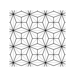
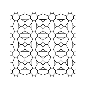
Figure 2: Illustrations for the main theorem 6.1 and its outline. Top row: the hexagonal and square-octagon lattices are probably the two most important lattices for which the theorem is applicable. Top left: the lozenge $L_{2}$ on the hexagonal lattice is determined by a 4-by-4 lozenge walk on the dual (in gray); the same notation directly interpreted as a planar domain, dual subgraph (on or inside the loop) as well as a primal subgraph (strictly inside). The reflection symmetry axis of the lozenge is dashed. Bottom row: a general “recipe” to produce lattices where Theorem 6.1 applies. Start from a lattice with the required symmetries and with maximum degree and maximum dual degree both at most $11$ (left). Draw its corner-to-face adjacency graph (middle). Then replace each vertex of degree $d$ of the latter with a little $d$-gon (right). The resulting graph (right) is cubic with maximal dual degree $11$, and has the same symmetries as the original one (left).

For the rest of this article, we fix the lattice $\mathbb{G}$ and the weights $\mathbf{c}_{e}$ (inexplicit constants may depend on these) and impose following assumptions (see Figure 2 for examples): $\mathbb{G}$ is a connected, countably infinite, locally finite graph. It is planar and bi-periodic (and comes with such an embedding), one of the translational symmetries being along the horizontal axis. The maximum degree for $\mathbb{G}$ is $3$ and for its dual $\mathbb{G}^{*}$ it is at most $11$. The graph $\mathbb{G}$ is invariant under reflection with respect to both horizontal and vertical axes. There is a discretization of either a square of side-length $n$ translational invariance steps (e.g., in the case of the square-octagon lattice), or a rhombus of side-length $n$ with angles $60^{\circ}$ and $120^{\circ}$ (e.g., in honeycomb lattice), such that both $\mathbb{G}$ and the discretized square (resp. rhombus) are invariant under reflection with respect to the diagonal line of the square (resp. the diagonal line between the $120^{\circ}$ angles of the rhombus). Finally, we assume throughout this section that $1\leq\mathbf{c}_{e}\leq 2$ for all $e\in\mathbb{E}$ and that $\mathbf{c}_{e}$ satisfy the same symmetries as the lattice $\mathbb{G}$. The main result of this section can now be stated.

Theorem 6.1

In the above setup, there exist $C,c>0$ such that for any finite $D\subset\mathbb{V}$ and $x\in D$ with $d_{\mathbb{G}}(x,D^{c})\geq 2$,

$$c\log d_{D}(x,\partial D)\leq\mathbb{E}^{\pm 1}_{D}[h(x)^{2}]\leq C\log d_{D}(x,\partial D),$$ (log-Var-deloc)

where the boundary condition $\pm 1$ is imposed on $\partial D$.

6.2 Outline for Theorem 6.1

The core of the proof of Theorem 6.1 is, in jargon, to deduce a dichotomy of level-line loop probabilities via a renormalization inequality. We now explain this jargon and show how it implies Theorem 6.1.

Let $L_{n}$ denote the discrete square/rhombus with side length $2n$ translational invariance steps. Let $\mathcal{O}_{\omega=1}(L_{n})$ denote the event that there is a loop path surrounding $L_{n}$ with $\omega=1$ on the edges, and let

$$a_{n}=\mathbb{P}_{L_{Rn}}^{\pm 1}[\mathcal{O}_{\omega=1}(L_{n})],$$ (5)

where $R$ is a constant that we fix to $R=3$ to facilitate the geometric arguments in the proof and the lozenges $L_{n}$ and $L_{Rn}$ are cocentric. The loop probability dichotomy is now stated as follows.

Theorem 6.2 (Loop probability dichotomy)

There exist $C,c,\alpha>0$ such that either

$$a_{n} \geq c\qquad\text{for all $n$},$$ (loop-deloc)

$$\text{or}\qquad a_{n} \leq C\exp(-cn^{\alpha})\qquad\text{for all $n$}.$$ (loop-loc)

This is indeed equivalent with the earlier dichotomies.

Theorem 6.3 (Three equivalent dichotomies)

i) If (loop-loc) occurs, then also (5.3) and (Var-loc) occur. ii) If (loop-deloc) occurs, then (log-Var-deloc) (and hence also  (Var-deloc) and (5.3)) occurs.

Theorem 6.3 is a fairly simple consequence of intermediate steps in the proof of Theorem 6.2; see Section 10. Let us now see how the two immediately imply Theorem 6.1:

Proof of Theorem 6.1

By Theorem 6.2, either (loop-loc) or (loop-deloc) occurs. In the first case, by Theorem 6.3, the variance is bounded (Var-loc), and in the second it diverges logarithmically (log-Var-deloc). On the other hand, by Theorem 5.4, the variance diverges, so (log-Var-deloc) holds.   $\square$

The main open question is thus to prove Theorem 6.2. This is done via the so-called renormalization inequality. For technical reasons, the inequality will be more conveniently derived for a quantity $b_{n}$ closely related to $a_{n}$.

Proposition 6.4 (Renormalization inequality)

There exists $C>0$ such that every $n$, at least one of the following two holds, where $R^{\prime}=14$:

$$\text{i)}\qquad b_{n}\geq\tfrac{1}{2C};\qquad\text{or}\qquad\text{ii)}\qquad b_{R^{\prime}n}\leq Cb_{n}^{2}.$$

Remark 6.5

With an adjustment of the constant $C$, the two alternatives can both be shown to imply $b_{R^{\prime}n}\leq C^{\prime}b_{n}^{2}$ (since $b_{R^{\prime}n}\leq 1$); the two-case formulation is nevertheless how the result is proven and used, and we hence persist to give this “suboptimal” formulation.

For completeness, we recall how the renormalization inequality implies the dichotomy of Theorem 6.2, even if this argument is very standard by now.

Proof of the dichotomy of Theorem 6.2 for $b_{n}$

Let us first study a subsequence of $n$:s that are powers of $R^{\prime}$, $n_{k}=(R^{\prime})^{k}$. By Proposition 6.4, this subsequence has the property that, if for some $k$ it holds true that $b_{n_{k}}<\tfrac{1}{\alpha C}$ for some $\alpha>2$, then also $b_{n_{k+1}}\leq Cb_{n_{k}}^{2}<\tfrac{1}{\alpha^{2}C}$ and, using this inductively, $b_{n_{k+\ell}}<\tfrac{1}{\alpha^{2^{\ell}}C}$.

Now, if $b_{n_{k}}\geq\tfrac{1}{2C}$ for all $k$, then the analogue of (loop-deloc) holds for $b_{n_{k}}$ along the subsequence $n_{k}$. If not, there exists $k_{0}$ such that $b_{n_{k_{0}}}<\tfrac{1}{2C}$, and by the previous paragraph,

$$b_{n_{k_{0}+\ell}}<\tfrac{1}{2^{2^{\ell}}C},\qquad\text{for all }\ell\in\mathbb{N}.$$

For $n=n_{k_{0}+\ell}$, one has $\ell=\log_{R^{\prime}}n-k_{0}$, and denoting $c=2^{-k_{0}}$ and $\alpha=\log_{R^{\prime}}2$, we have

$$b_{n}<\tfrac{1}{C}2^{-cn^{\alpha}}\qquad\text{for $n$ of the form }n=n_{k_{0}+\ell},$$

i.e., the analogue of (loop-loc) holds for $b_{n_{k}}$ along the subsequence $n_{k}$.

It now remains to “fill the subsequence” which can be done, e.g., via a standard “necklace argument”: for any $N\in[n_{k+2},n_{k+3}]$ and $n\in[n_{k},n_{k+1}]$, a loop as in the definition of $b_{N}$ can be generated by a fixed number $\ell$ of translated loops of the size in $b_{n}$. By the FKG, then, $b_{N}\geq(b_{n})^{\ell}$. Case (i) for $n_{k}$ then implies case (i) for all $N$ via the special case $b_{N}\geq(b_{n_{k+1}})^{\ell}$. Case (ii) for $n_{k}$ implies case (ii) for all $n$ via $b_{n}\leq(b_{n_{k+2}})^{1/\ell}$. This concludes the proof.   $\square$

The remaining questions are thus to prove Proposition 6.4 and — simpler — Theorem 6.3. This is done in the following four sections.

7 Crossings in discrete topological quardilaterals

7.1 Quadrilaterals

A simply-connected (discrete) domain $D=(V,E)$ of $\mathbb{G}$ consists of the vertices and edges that lie inside a simple closed loop $\ell$ on the dual $\mathbb{G}^{*}$. Given such $D$ and $\ell$, and let $\mathsf{bl},\mathsf{br},\mathsf{tr},\mathsf{tl}$ (standing for bottom-left, bottom-right etc.) be four distinct marked faces on $\ell$, in counterclockwise order. The tuple $(D;\mathsf{bl},\mathsf{br},\mathsf{tr},\mathsf{tl})$ is called a discrete topological quadrilateral, or a quad, for short (if the marked faces are clear in the context, we will simply refer to “the quad $D$”). We denote by $E_{\mathsf{left}}^{*}$ the dual-edges on the counter-clockwise arc of $\ell$ between $\mathsf{tl}$ and $\mathsf{bl}$, by $E_{\mathsf{left}}$ the primal-edges (of $\mathbb{G}\setminus D$) crossing them, by $V_{\mathsf{left}}^{*}$ the dual-vertices on the counterclockwise arc of $\ell$ between or including $\mathsf{tl}$ and $\mathsf{bl}$, and by $V_{\mathsf{left}}$ or the vertices of $F$ adjacent to $E_{\mathsf{left}}$ in $\mathbb{G}$. The $\mathsf{bottom}$, $\mathsf{right}$, and $\mathsf{top}$ sides are given similar notations.

For $A,B\subset\mathbb{V}$, denote $A\stackrel{{\scriptstyle\mathcal{E}}}{{\longleftrightarrow}}B$ if there is a path connecting $A$ and $B$ on $\mathbb{G}$ and using only edges of $\mathcal{E}\subset\mathbb{E}$. Analogous connections on the dual $\mathbb{G}^{*}$ are denoted by $\longleftrightarrow_{*}$.

Lemma 7.1

Let $D=(V,E)$ be a quad on $\mathbb{G}$ and $\mathcal{E}$ a (random) subset of $E$; then

$$\{V_{\mathsf{left}}\stackrel{{\scriptstyle\mathcal{E}}}{{\longleftrightarrow}}V_{\mathsf{right}}\}^{c} =\{V_{\mathsf{bottom}}^{*}\stackrel{{\scriptstyle(\mathcal{E}^{c})^{*}}}{{\longleftrightarrow}}_{*}V_{\mathsf{top}}^{*}\}\qquad\text{and}$$ (6)

$$\{V_{\mathsf{left}}\stackrel{{\scriptstyle\mathcal{E}}}{{\longleftrightarrow}}V_{\mathsf{right}}\} \subset\{V_{\mathsf{left}}^{*}\stackrel{{\scriptstyle\mathcal{E}^{*}}}{{\longleftrightarrow}}_{*}V_{\mathsf{right}}^{*}\}.$$ (7)

Proof

Equation (6) is a standard duality property. For (7), on the occurrence of $\{V_{\mathsf{left}}\stackrel{{\scriptstyle\mathcal{E}}}{{\longleftrightarrow}}V_{\mathsf{right}}\}$, let $\gamma$ be a path on $\mathbb{G}$ with first edge on $E_{\mathsf{left}}$, last on $E_{\mathsf{right}}$, and the remaining edges being in $\mathcal{E}\subset D$ and generating this event. Analogously, on $\{V_{\mathsf{left}}^{*}\stackrel{{\scriptstyle\mathcal{E}^{*}}}{{\longleftrightarrow}}_{*}V_{\mathsf{right}}^{*}\}^{c}=\{V_{\mathsf{bottom}}\stackrel{{\scriptstyle\mathcal{E}^{c}}}{{\longleftrightarrow}}V_{\mathsf{top}}\}$ (where we used (6)), let $\gamma^{\prime}$ on $\mathbb{G}$ have its first edge on $E_{\mathsf{bottom}}$, last on $E_{\mathsf{top}}$, and the rest in $\mathcal{E}^{c}$ and generating the latter event. We will show that such $\gamma$ and $\gamma^{\prime}$ cannot co-exist, and hence $\{V_{\mathsf{left}}\stackrel{{\scriptstyle\mathcal{E}}}{{\longleftrightarrow}}V_{\mathsf{right}}\}\subset\{V_{\mathsf{left}}^{*}\stackrel{{\scriptstyle\mathcal{E}^{*}}}{{\longleftrightarrow}}_{*}V_{\mathsf{right}}^{*}\}^{cc}$, and the proof is complete. If $\gamma$ and $\gamma^{\prime}$ did co-exist, then by topological obstruction, they must share a vertex in $D$. On the other hand, they are manifestly edge-disjoint and hence also vertex-disjoint, possibly apart from endpoint vertices. But all non-endpoint vertices are in $D$, so they cannot share a vertex in $D$, a contradiction.   $\square$

7.2 Crossings of symmetric quads

Let $\tau$ be a symmetry of the lattice $\mathbb{G}$ (e.g., a reflection with respect to the vertical axis). We say that $(D;\mathsf{bl},\mathsf{br},\mathsf{tr},\mathsf{tl})$ is symmetric with respect to $\tau$, if $\tau(D)=D$ and furthermore, $\tau$ fixes two of the corner faces, and exchanges the remaining two. Then, for a boundary condition $\xi:\partial D\to\mathbb{Z}_{\mathrm{odd}}$, denote by $\tau.\xi$ the boundary condition $\xi\circ\tau^{-1}$. In this situation $2-\xi\succeq\tau.\xi$ means, informally speaking, the boundary condition “tends to be more below $1$ than above”. The following lemma formalizes this intuition.

Below an in continuation, we denote by $\{h\omega\leq 0\}$ (resp. $\{h\omega\geq 1\}$) the set of edges $e=\langle u,v\rangle$ on which $h(u)\omega(e),h(v)\omega(e)\leq 0$, i.e., $h(u),h(v)\leq 1$ and if $h(u)=h(v)=1$ then also $B_{e}=0$ (resp. its complement, on which $h(u)\omega(e),h(v)\omega(e)\geq 1$, i.e., $h(u),h(v)\geq 1$ and if $h(u)=h(v)=1$ then also $B_{e}=1$). With a slight abuse of notation, we also denote, e.g., $\{h\omega\leq 0\}^{*}\subset\mathbb{E}^{*}$ simply by $\{h\omega\leq 0\}$. The edges $\{h\omega\geq 0\}$ and their complement $\{h\omega\leq-1\}$ are defined analogously.

Lemma 7.2

Let $D$ be symmetric quad with respect to $\tau$ and $\xi$ an interval-valued boundary condition on $\partial D$, such that $2-\xi\succeq\tau.\xi$. Then,

$$\mathbb{P}^{\xi}_{D}[V_{\mathsf{left}}^{*}\stackrel{{\scriptstyle h\omega\leq 0}}{{\longleftrightarrow}}_{*}V_{\mathsf{right}}^{*}]\geq 1/2.$$

Proof

Note that $\{V_{\mathsf{left}}^{*}\stackrel{{\scriptstyle h\omega\leq 0}}{{\longleftrightarrow}}_{*}V_{\mathsf{right}}^{*}\}^{c}=\{V_{\mathsf{bottom}}\stackrel{{\scriptstyle h\omega\geq 1}}{{\longleftrightarrow}}V_{\mathsf{top}}\}$, by (6). Combining with the symmetry,

$$1-\mathbb{P}^{\xi}_{D}[V_{\mathsf{left}}^{*}\stackrel{{\scriptstyle h\omega\leq 0}}{{\longleftrightarrow}}_{*}V_{\mathsf{right}}^{*}] =\mathbb{P}^{\xi}_{D}[V_{\mathsf{bottom}}\stackrel{{\scriptstyle h\omega\geq 1}}{{\longleftrightarrow}}V_{\mathsf{top}}]$$

$$=\mathbb{P}^{\tau.\xi}_{D}[V_{\mathsf{left}}\stackrel{{\scriptstyle h\omega\geq 1}}{{\longleftrightarrow}}V_{\mathsf{right}}].$$

Next, a path satisfying $h\omega\geq 1$ equivalently means that $h\geq 1$ on all vertices and, additionally, $B_{e}=1$ on edges between two heights $1$. The existence of such paths is manifestly an increasing event in $(h,B)$, so by the FKG,

$$\mathbb{P}^{\tau.\xi}_{D}[V_{\mathsf{left}}\stackrel{{\scriptstyle h\omega\geq 1}}{{\longleftrightarrow}}V_{\mathsf{right}}]\leq\mathbb{P}^{2-\xi}_{D}[V_{\mathsf{left}}\stackrel{{\scriptstyle h\omega\geq 1}}{{\longleftrightarrow}}V_{\mathsf{right}}].$$

Next, given $(h,B,\omega)$ under $\mathbb{P}^{2-\xi}_{D}$, we define $\tilde{h}=2-h$ (so that $\tilde{h}\sim\mathbb{P}^{\xi}_{D}$). Then, define a coupling measure $\mathbb{P}$ to also include independent $\mathsf{Ber}(1-1/\mathbf{c}_{e})$ variables $(\tilde{B}_{e})_{e\in E}$ (i.e., with the same law as $B_{e}$), each $\tilde{B}_{e}$ coupled to $B_{e}$ so that $B_{e}=1\Rightarrow\tilde{B}_{e}=0$. Finally define $\tilde{\omega}$ from $\tilde{h}$ and $\tilde{B}$ in the usual manner (so that $(\tilde{h},\tilde{B},\tilde{\omega})\sim\mathbb{P}^{\xi}_{D}$). In this coupling $\mathbb{P}$, a path of $h\geq 1$ with additionally $B_{e}=1$ on edges between two heights $1$ is also a path of $\tilde{h}\leq 1$ with additionally $\tilde{B}_{e}=0$ on edges between two heights $1$, i.e.,

$$\{V_{\mathsf{left}}\stackrel{{\scriptstyle h\omega\geq 1}}{{\longleftrightarrow}}V_{\mathsf{right}}\}\subset\{V_{\mathsf{left}}\stackrel{{\scriptstyle\tilde{h}\tilde{\omega}\leq 0}}{{\longleftrightarrow}}V_{\mathsf{right}}\}.$$

Finally, we observe that by (7)

$$\{V_{\mathsf{left}}\stackrel{{\scriptstyle\tilde{h}\tilde{\omega}\leq 0}}{{\longleftrightarrow}}V_{\mathsf{right}}\}\subset\{V_{\mathsf{left}}^{*}\stackrel{{\scriptstyle\tilde{h}\tilde{\omega}\leq 0}}{{\longleftrightarrow}}_{*}V_{\mathsf{right}}^{*}\}.$$

With the two previous set inclusions and the observation $(\tilde{h},\tilde{B},\tilde{\omega})\sim\mathbb{P}^{\xi}_{D}$, we have

$$\mathbb{P}^{2-\xi}_{D}[V_{\mathsf{left}}\stackrel{{\scriptstyle h\omega\geq 1}}{{\longleftrightarrow}}V_{\mathsf{right}}]=\mathbb{P}[V_{\mathsf{left}}\stackrel{{\scriptstyle h\omega\geq 1}}{{\longleftrightarrow}}V_{\mathsf{right}}]\leq\mathbb{P}[V_{\mathsf{left}}^{*}\stackrel{{\scriptstyle\tilde{h}\tilde{\omega}\leq 0}}{{\longleftrightarrow}}_{*}V_{\mathsf{right}}^{*}]=\mathbb{P}^{\xi}_{D}[V_{\mathsf{left}}^{*}\stackrel{{\scriptstyle h\omega\leq 0}}{{\longleftrightarrow}}_{*}V_{\mathsf{right}}^{*}].$$

Combining all the displayed (non-set) inequalities now yields the claim.   $\square$

7.3 Comparing symmetric quads to narrower ones

Note that the intersection graph $Q\cap D$ of two simply-connected domains $Q$ and $D$ consists of connected components $C$ that are themselves simply-connected discrete domains, each with a bounding dual-loop $\ell(C)$ consisting of dual-edges on $\ell(Q)$ or $\ell(D)$. Suppose now that $Q$ has a quad structure, that $C$ contains a vertical primal crossing of $Q$, and that $\ell(C)\setminus\ell(D)\subset E^{*}_{\mathsf{top}}(Q)\cup E^{*}_{\mathsf{bot}}(Q)$. Then, exactly two segments of $\ell(C)\cap\ell(D)$ cross $Q$ vertically (potentially overlapping with $E^{*}_{\mathsf{left}}(Q)\cup E^{*}_{\mathsf{right}}(Q)$), one from bottom to top and one from top to bottom (orienting $\ell(C)$ counter-clockwise). We call these the left and right walls of $C$, respectively. Finally, if also $D$ has a quad structure, we say that $D$ is narrower than $Q$, if there exists such a $C$ and furthermore $\ell(C)\setminus\ell(Q)\subset E^{*}_{\mathsf{left}}(D)\cup E^{*}_{\mathsf{right}}(D)$ and the left (resp. right) wall of $C$ is contained in $E^{*}_{\mathsf{left}}(D)$ (resp. $E^{*}_{\mathsf{right}}(D)$).

Lemma 7.3

Let $D$ be a quad that is narrower than a symmetric quad $Q$ and $\xi$ an interval-valued boundary condition on $\partial D$ which is $\{\pm 1\}$ on $V_{\mathsf{left}}(D)\cup V_{\mathsf{right}}(D)$ and $\xi\preceq\{1,3\}$ on the rest of $\partial D$. Then, we have

$$\mathbb{P}^{\xi}_{D}[V_{\mathsf{left}}^{*}(D)\stackrel{{\scriptstyle h\omega\leq 0}}{{\longleftrightarrow}}_{*}V_{\mathsf{right}}^{*}(D)]\geq\tfrac{1}{2}.$$

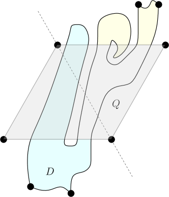
Figure 3: A schematic illustration for the proof of Lemma 7.3. The discretized lozenge $Q$ is a symmetric quad with respect to the reflection $\tau$ around its diagonal line (dashed). The present quad $D$ is narrower than $Q$, and there is a unique component $C$ of $D\cap Q$ inducing this structure (uncoloured). The components of $D\setminus C$ are adjacent to $C$ either via the top of $Q$ ($D_{\mathsf{top}}$, yellow), or via the bottom of $Q$ ($D_{\mathsf{bottom}}$, blue). The glueing $Q\bigcupplus D_{\mathsf{top}}\bigcupplus D_{\mathsf{bottom}}\bigcupplus\tau(D_{\mathsf{top}})\bigcupplus\tau(D_{\mathsf{bottom}})$ will produce a “discrete Riemann surface” which is a symmetric quad (with the same corners as $Q$).

Proof

Note first that $\{V_{\mathsf{left}}^{*}(D)\stackrel{{\scriptstyle h\omega\leq 0}}{{\longleftrightarrow}}_{*}V_{\mathsf{right}}^{*}(D)\}$ is a decreasing event in $(h,B)$. It thus suffices to prove the claim assuming that $\xi=\{1,3\}$ on $\partial D\setminus V_{\mathsf{left}}(D)\cup V_{\mathsf{right}}(D)$. With this boundary condition, we have $\{V_{\mathsf{left}}^{*}(D)\stackrel{{\scriptstyle h\omega\leq 0}}{{\longleftrightarrow}}_{*}V_{\mathsf{right}}^{*}(D)\}=\{V_{\mathsf{left}}^{*}(D)\stackrel{{\scriptstyle\omega=0}}{{\longleftrightarrow}}_{*}V_{\mathsf{right}}^{*}(D)\}$, which is is manifestly a decreasing event in $(|h|,\omega)$.

We will now aim to use the FKG for $(|h|,\omega)$. Let $D_{\mathsf{top}}$ (resp. $D_{\mathsf{bottom}}$) be the components of $D\setminus C$ that are adjacent to $C$ via the top (resp. bottom) of $Q$ (so $D\setminus C$ consists of $D_{\mathsf{top}}$ and $D_{\mathsf{bottom}}$); see Figure 3. Note that the connected components of $D\setminus C$ are discrete simply-connected domains, and every component of $D_{\mathsf{top}}$ contains exactly one sub-segment of $\ell(C)\cap E^{*}_{\mathsf{top}}(Q)$ on its bounding dual loop; we let $Q\bigcupplus D_{\mathsf{top}}$ denote the operation of gluing the graph $D_{\mathsf{top}}$ to the graph $Q$ along these shared boundary segments on $E^{*}_{\mathsf{top}}(Q)$. Hence the graph $Q\bigcupplus D_{\mathsf{top}}$ is planar and has locally a “honeycomb structure”, but it may not be embeddable to the plane so that this honeycomb structure remains embedded as regular hexagons. In what follows, it is however more beneficial to think of $Q\bigcupplus D_{\mathsf{top}}$ as a “discrete Riemann surface” and embed it in a “honeycomb manner”. Define via analogous gluing

$$D^{\prime}=Q\bigcupplus D_{\mathsf{top}}\bigcupplus D_{\mathsf{bottom}}\bigcupplus\tau(D_{\mathsf{top}})\bigcupplus\tau(D_{\mathsf{bottom}}).$$

With a slight abuse of notation, $\tau$ can be seen as a graph isomorphism from $D^{\prime}$ to itself. Give $D^{\prime}$ a quad structure by marking the corner faces of $Q$, and let $\xi^{\prime}$ be $\xi^{\prime}=\{\pm 1\}$ on $V_{\mathsf{left}}(D^{\prime})\cup V_{\mathsf{right}}(D^{\prime})$ and $\xi^{\prime}=\{1,3\}$ on the rest of $\partial D^{\prime}$. Similarly as above, with this boundary condition,

$$\{V_{\mathsf{left}}^{*}(D^{\prime})\stackrel{{\scriptstyle h\omega\leq 0}}{{\longleftrightarrow}}_{*}V_{\mathsf{right}}^{*}(D^{\prime})\}=\{V_{\mathsf{left}}^{*}(D^{\prime})\stackrel{{\scriptstyle\omega=0}}{{\longleftrightarrow}}_{*}V_{\mathsf{right}}^{*}(D^{\prime})\}.$$

Lemma 7.2 (actually, a slight extension with $\tau$ being a graph isomorphism rather than a symmetry of $\mathbb{G}$) yields

$$\mathbb{P}^{\xi^{\prime}}_{D^{\prime}}[V_{\mathsf{left}}^{*}(D^{\prime})\stackrel{{\scriptstyle h\omega\leq 0}}{{\longleftrightarrow}}_{*}V_{\mathsf{right}}^{*}(D^{\prime})]\geq\tfrac{1}{2},$$

and the FKG and CBC for $(|h|,\omega)$ yield

$$\mathbb{P}^{\xi}_{D}[V_{\mathsf{left}}^{*}(D)\stackrel{{\scriptstyle\omega=0}}{{\longleftrightarrow}}_{*}V_{\mathsf{right}}^{*}(D)]\geq\mathbb{P}^{\xi^{\prime}}_{D^{\prime}}[V_{\mathsf{left}}^{*}(D^{\prime})\stackrel{{\scriptstyle\omega=0}}{{\longleftrightarrow}}_{*}V_{\mathsf{right}}^{*}(D^{\prime})].$$

Combining the three previously displayed equations proves the claim.   $\square$

We will need another similar result, however stronger in the sense that the crossings to be found are inside the small domain $C$; the price to pay for this extra information is the assumption that the domain $C$ is on the bottom of $D$, in the sense that $E^{*}_{\mathsf{bottom}}(D)\subset\ell(C)$ (or on the top, defined analogously). The proof is similar to Lemma 7.2 but a bit more involved; we postpone it to Appendix C.

Lemma 7.4

Let $D$ be a quad that is narrower than a symmetric quad $Q$, with a component $C$ inducing this narrower structure being on the bottom of $D$; let $\xi$ be an interval-valued boundary condition on $\partial D$ which is $\{\pm 1\}$ on $V_{\mathsf{left}}(D)\cup V_{\mathsf{right}}(D)$ and $\xi\preceq\{5,7\}$ on the rest of $\partial D$, and denote by $\mathcal{E}(h,B)$ the set of edges between heights $h\leq 3$ with additionally $B_{e}=0$ for edges between two heights $3$. We then have

$$\mathbb{P}^{\xi}_{D}[V_{\mathsf{left}}^{*}(D)\stackrel{{\scriptstyle\mathcal{E}(h,B)^{*}\cap C}}{{\longleftrightarrow}}_{*}V_{\mathsf{right}}^{*}(D)]\geq\tfrac{1}{2}.$$

The main result of this section is the following.

Corollary 7.5

Let $D$ be a quad that is narrower than three symmetric quads $Q_{1}$, $Q_{2}$, $Q_{3}$, furthermore so that the respective connected components $C_{i}\subset Q_{i}\cap D$, $i\in\{1,2,3\}$, that generate the narrower structure can be chosen disjoint and $C_{1}$ on the bottom and $C_{3}$ on the top of $D$. Let $\xi$ be an interval-valued boundary condition on $\partial D$ which is $\{\pm 1\}$ on $V_{\mathsf{left}}(D)\cup V_{\mathsf{right}}(D)$ and $\xi\preceq\{5,7\}$ on the rest. Then, we have

$$\mathbb{P}^{\xi}_{D}[V_{\mathsf{left}}^{*}(D)\stackrel{{\scriptstyle h\omega\leq 0}}{{\longleftrightarrow}}_{*}V_{\mathsf{right}}^{*}(D)]\geq\tfrac{1}{8}.$$

Proof

Again, it suffices to consider the maximal $\xi$ allowed in the statement. Define $\mathcal{E}(h,B)$ as in Lemma C.1; by that lemma,

$$\mathbb{P}^{\xi}_{D}[V_{\mathsf{left}}^{*}(D)\stackrel{{\scriptstyle\mathcal{E}(h,B)^{*}\cap C_{1}}}{{\longleftrightarrow}}_{*}V_{\mathsf{right}}^{*}(D)],\;\mathbb{P}^{\xi}_{D}[V_{\mathsf{left}}^{*}(D)\stackrel{{\scriptstyle\mathcal{E}(h,B)^{*}\cap C_{3}}}{{\longleftrightarrow}}_{*}V_{\mathsf{right}}^{*}(D)]\geq\tfrac{1}{2}.$$

Denote the two events on the left by $\mathcal{H}_{1}$ and $\mathcal{H}_{3}$, respectively. Since both are decreasing in $(h,B)$, FKG gives

$$\mathbb{P}^{\xi}_{D}[\mathcal{H}_{1}\cap\mathcal{H}_{3}]\geq 1/4,$$

and it thus suffices to show that

$$\mathbb{P}^{\xi}_{D}[V_{\mathsf{left}}^{*}(D)\stackrel{{\scriptstyle h\omega\leq 0}}{{\longleftrightarrow}}_{*}V_{\mathsf{right}}^{*}(D)\;|\;\mathcal{H}_{1}\cap\mathcal{H}_{3}]\geq 1/2.$$

For this purpose, set $\tilde{h}=2-h$ and define $\tilde{\omega}$ via $\tilde{h}$ and $B_{e}$ in the usual manner; note that $\mathcal{E}(h,B)=\{\tilde{h}\tilde{\omega}\geq 0\}$. To reveal whether $\mathcal{H}_{1}\cap\mathcal{H}_{3}$ occurs, we explore the cluster of $\tilde{h}\tilde{\omega}<0$ in $C_{1}$ (resp. $C_{3}$) adjacent to the bottom (resp. top) boundary of $D$: formally, let $V_{1}$ consist of $V_{\mathsf{bottom}}$ and the vertices of $D$ connected to $V_{\mathsf{bottom}}$ by edges of $\tilde{h}\tilde{\omega}<0$, and let $E_{1}$ consist of these primal-edges and the primal-edges crossing the dual-paths bounding the former. Define $V_{3}$ and $E_{3}$ analogously via $C_{3}$. Now, the event $V_{1}=A_{1},E_{1}=B_{1}$ is determined by $\tilde{h}_{|A_{1}},\tilde{\omega}_{|B_{1}}$; let $\Xi$ be the set of $(A_{1},B_{1},A_{3},B_{3},\alpha_{1},\nu_{1},\alpha_{3},\nu_{3})$ such that $\{\tilde{h}_{|A_{1}}=\alpha_{1},\tilde{\omega}_{|B_{1}}=\nu_{1},\tilde{h}_{|A_{3}}=\alpha_{3},\tilde{\omega}_{|B_{3}}=\nu_{3}\}$ induces $\mathcal{H}_{1}\cap\mathcal{H}_{3}$ with $V_{1}=A_{1},E_{1}=B_{1},V_{3}=A_{3},E_{1}=B_{3}$. Then,

$$\mathbb{P}^{\xi}_{D} [\mathcal{H}_{1}\cap\mathcal{H}_{3}]=\sum_{\Xi}\mathbb{P}^{\xi}_{D}[\tilde{h}_{|A_{1}}=\alpha_{1},\tilde{\omega}_{|B_{1}}=\nu_{1},\tilde{h}_{|A_{3}}=\alpha_{3},\tilde{\omega}_{|B_{3}}=\nu_{3}]$$

$$\mathbb{P}^{\xi}_{D} [V_{\mathsf{left}}^{*}(D)\stackrel{{\scriptstyle h\omega\leq 0}}{{\longleftrightarrow}}_{*}V_{\mathsf{right}}^{*}(D)\cap\mathcal{H}_{1}\cap\mathcal{H}_{3}]$$

$$=\sum_{\Xi}\mathbb{P}^{\xi}_{D}[\tilde{h}_{|A_{1}}=\alpha_{1},\tilde{\omega}_{|B_{1}}=\nu_{1},\tilde{h}_{|A_{3}}=\alpha_{3},\tilde{\omega}_{|B_{3}}=\nu_{3}]$$

$$\qquad\mathbb{P}^{\xi}_{D}[V_{\mathsf{left}}^{*}(D)\stackrel{{\scriptstyle h\omega\leq 0}}{{\longleftrightarrow}}_{*}V_{\mathsf{right}}^{*}(D)\;|\;\tilde{h}_{|A_{1}}=\alpha_{1},\tilde{\omega}_{|B_{1}}=\nu_{1},\tilde{h}_{|A_{3}}=\alpha_{3},\tilde{\omega}_{|B_{3}}=\nu_{3}],$$

and it suffices to show that the last conditional probability is at least $1/2$ for all $(A_{1},B_{1},A_{3},$ $B_{3},\alpha_{1},\nu_{1},\alpha_{3},\nu_{3})$. Note that the component of unexplored vertices $V\setminus A_{1}\setminus A_{3}$ that contains $C_{2}$ is a simply-connected discrete domain $D^{\prime}$ restricted by $\ell(D)$ and the dual-paths bounding the $\tilde{h}\tilde{\omega}<0$ clusters. By SMP (Lemma 4.5), the conditional measure $\mathbb{P}^{\xi}_{D}[\cdot\;|\;\tilde{h}_{|A_{1}}=\alpha_{1},\tilde{\omega}_{|B_{1}}=\nu_{1},\tilde{h}_{|A_{3}}=\alpha_{3},\tilde{\omega}_{|B_{3}}=\nu_{3}]$ restricted to this component is a random Lipschitz model, with the boundary condition $\xi^{\prime}$ given by $h\in\{\pm 1\}$ on $E^{*}_{\mathsf{left}}(D)$ and $E^{*}_{\mathsf{right}}(D)$, $h\in\{1,3\}$ on the unexplored tips of $\tilde{\omega}=0$ edges, and given $\alpha_{1}$ and $\alpha_{3}$ the top and bottom vertices of $V$ from which the exploration of $\tilde{h}\tilde{\omega}<0$ never proceeded forward (whence $\xi^{\prime}\leq 1$ on these vertices). This boundary condition is suited for the application of Lemma 7.2, giving

$$\mathbb{P}^{\xi^{\prime}}_{D^{\prime}}[V_{\mathsf{left}}^{*}(D)\stackrel{{\scriptstyle h\omega\leq 0}}{{\longleftrightarrow}}_{*}V_{\mathsf{right}}^{*}(D)]\geq 1/2.$$

This concludes the proof.   $\square$

8 The Pushing Theorem

8.1 Statement

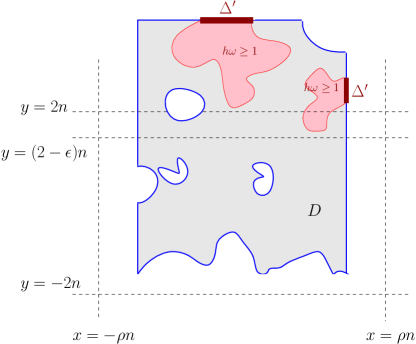
Figure 4: Illustration for Proposition 8.2, through which Theorem 8.1 is typically applied.

We will next use the crossing probabilities in symmetric quads to derive a fairly general uniformly positive crossing probability for discrete rectangles.

A (discrete) rectangle $R_{n,m}$ is a discrete topological quadrilateral, centered at the origin face and extending $n$ horizontal (resp. $m$ vertical) translational periods of $\mathbb{G}$ to both left and right (resp. both up and down), and invariant under reflection around the horizontal axis. For an explicit definition the honeycomb lattice case, suppose that $\mathbb{G}$ is embedded in the complex plane so that the normal vectors of the sides of a hexagon are the sixth roots of unity and the origin is in a middle of an origin face. Scale the embedding to side length $1/3$ for the hexagons; hence the horizontal lines $y\in\mathbb{Z}$ cross the midpoints of every second a row of faces (depict the vertical translational period), and the distance of two neighbouring midpoints (the horizontal translational period) is $1/\sqrt{3}$. Then let $R_{n,m}$ denote the rectangle consisting of faces with midpoints in $[-1/\sqrt{3}\cdot n,1/\sqrt{3}\cdot n]\times[-m,m]$, thus of width $2n+1$ hexagons and height $4m+1$ rows. For another example, on the square-octagon lattice with origin in the middle of and octagonal face and a translational symmetry $\mathbb{Z}^{2}$, $R_{n,m}$ would consist of the faces with midpoints in $[-n,n]\times[-m,m]$.

Horizontal and vertical crossings of a rectangle $R$ by edge set $\mathcal{E}$ are denoted $\mathcal{H}_{\mathcal{E}}(R)$ and $\mathcal{V}_{\mathcal{E}}(R)$, respectively, and dual-crossings by $\mathcal{H}^{*}_{\mathcal{E}}(R)$ and $\mathcal{V}^{*}_{\mathcal{E}}(R)$.

Theorem 8.1

For any $\rho>0$, there exists $c=c(\rho)$ such that the following holds for any $n$. Let $D=(V,E)$ be a connected subgraph of $\mathbb{G}$, generated by its vertices and invariant under reflection $\tau$ with respect to the horizontal axis. Let $\xi\preceq\{5,7\}$ be an interval-valued boundary condition on $\partial D$, such that $2-\xi\succeq\tau.\xi$ and $\xi\preceq\{\pm 1\}$ on $\partial D\cap R_{\rho n,n}$. Then, we have

$$\mathbb{P}_{D}^{\xi}[\mathcal{V}_{h\omega\geq 1}(R_{\rho n,n})]\leq 1-c.$$

8.2 Consequences

Let us start with an introductory example that we don’t formulate as a separate corollary. Set $D=R_{\rho n,3n}$, $R=R_{\rho n,n}$, and let $\xi$ be set-valued $\{1,3\}$ on the top boundary of $D$ and $\{\pm 1\}$ on the side and bottom boundaries. The above theorem then applies, so $\mathbb{P}_{D}^{\xi}[\mathcal{H}^{*}_{h\omega\leq 0}(R)]>c$. Note also that due to the boundary condition,

$$\mathcal{H}^{*}_{h\omega\leq 0}(R)\subset\mathcal{H}^{*}_{h\omega\leq 0}(R_{+})=\mathcal{H}^{*}_{\omega=0}(R_{+}),$$

where $R_{+}$ denotes the two-thirds of $D$ that are in or above $R$. Now, to detect the event $\mathcal{H}^{*}_{\omega=0}(R_{+})$, explore the primal-clusters of $\omega$ adjacent to below $R_{+}$, and their top boundary, i.e., the lowest dual-crossing generating $\mathcal{H}^{*}_{\omega=0}(R_{+})$. By SMP (Lemma 4.5) this “pushes the $\{\pm 1\}$ boundary condition above the bottom of $R_{+}$”, hence the name of the theorem.

Let $\{y\leq m\}$ denote the set of vertices with vertical coordinate at most $m$ vertical translational periods (generalizing the case of the honeycomb lattice, where the vertical period is one length unit). The idea of the above example holds in a larger generality (see Figure 4):

Proposition 8.2

For every $\rho,\epsilon>0$ and $k\in\mathbb{N}$, there exists $c=c(\rho,\epsilon,k)$ such that the following holds for all $n>k/\epsilon$. Let $D$ be a connected subgraph of $\mathbb{G}$, generated by its vertices and contained entirely between the vertical lines $x=\pm\rho n$ horizontal periods and entirely above the horizontal line $y=-2n$ vertical periods. Let $\Delta^{\prime}\subset\partial D$ be a set of boundary vertices entirely above the horizontal line $y=2n$ and let $\xi$ be an interval-valued boundary condition on $\partial D$ taking values $\preceq\{2k\pm 1\}$ on $\Delta^{\prime}$ and $\xi\preceq\{\pm 1\}$ on $\partial D\setminus\Delta^{\prime}$. Then,

$$\mathbb{P}_{D}^{\xi}[\Delta^{\prime}\stackrel{{\scriptstyle h\omega\geq 1}}{{\longleftrightarrow}}\{y\leq(2-\epsilon)n\}]\leq 1-c.$$

We work towards the proof of this result via intermediate steps.

Lemma 8.3

For every $\rho$, there exists $c=c(\rho)$ such that the following holds for all $n$. Let $D$ and $\Delta^{\prime}$ be as above, and let $\xi$ be an interval-valued boundary condition on $\partial D$, being $\preceq\{1,3\}$ on $\Delta^{\prime}$ and $\xi\preceq\{\pm 1\}$ on $\partial D\setminus\Delta^{\prime}$. Then,

$$\mathbb{P}_{D}^{\xi}[\Delta^{\prime}\stackrel{{\scriptstyle h\omega\geq 1}}{{\longleftrightarrow}}\{y\leq-n\}]\leq 1-c.$$

Proof

Let us start by easy simplifying observations. First, if $D$ does not contain any vertical crossing of $R$, then the claim is trivial, so we assume it does. Second, the event $\{\Delta^{\prime}\stackrel{{\scriptstyle h\omega\geq 1}}{{\longleftrightarrow}}\{y\leq-n\}\}$ is increasing in $(h,B)$, so it suffices to prove the claim for the maximal boundary condition $\xi$ allowed by the assumptions, i.e., we may assume $\xi_{|\Delta^{\prime}}=\{1,3\}$ and $\xi_{|\partial D\setminus\Delta^{\prime}}=\{\pm 1\}$.

Let $\tau$ now denote the reflection with respect to the horizontal axis. By the first simplifying assumption, $D^{\prime}:=D\cup\tau(D)$ is a connected subgraph of $\mathbb{G}$. Furthermore, $\tau(D)$ remains below the line $y=2n$, so $\Delta^{\prime}\subset\partial D^{\prime}$. Let $\xi^{\prime}$ be the boundary condition on $\partial D^{\prime}$ given by $\xi^{\prime}_{|\Delta^{\prime}}=\{1,3\}$ and $\xi^{\prime}_{|\partial D^{\prime}\setminus\Delta^{\prime}}=\{\pm 1\}$. Next, we compute

$$\mathbb{P}_{D}^{\xi}[\Delta^{\prime}\stackrel{{\scriptstyle h\omega\geq 1}}{{\longleftrightarrow}}\{y\leq-n\}] =\mathbb{P}_{D}^{\xi}[\Delta^{\prime}\stackrel{{\scriptstyle\omega=1}}{{\longleftrightarrow}}\{y\leq-n\}]\qquad\text{(due to boundary condition)}$$

$$\leq\mathbb{P}_{D^{\prime}}^{\xi^{\prime}}[\Delta^{\prime}\stackrel{{\scriptstyle\omega=1}}{{\longleftrightarrow}}\{y\leq-n\}]\qquad\text{(by FKG for $(|h|,\omega)$)}$$

$$=\mathbb{P}_{D^{\prime}}^{\xi^{\prime}}[\Delta^{\prime}\stackrel{{\scriptstyle h\omega\geq 1}}{{\longleftrightarrow}}\{y\leq-n\}]\qquad\text{(due to boundary condition)}$$

$$\leq\mathbb{P}_{D^{\prime}}^{\xi^{\prime}}[\mathcal{V}_{h\omega\geq 1}(R_{\rho n,n})]\qquad\text{(by geometric setup)}$$

$$\leq 1-c(\rho)\qquad\text{(by Theorem\leavevmode\nobreak\ \ref{prop:pushing})}.$$

This concludes the proof.   $\square$

Lemma 8.4

For every $\rho,\epsilon>0$, there exists $c=c(\rho,\epsilon)$ such that the following holds for all $n>1/\epsilon$. Let $D$, $\Delta^{\prime}$, and $\xi$ be as in the previous lemma. Then,

$$\mathbb{P}_{D}^{\xi}[\Delta^{\prime}\stackrel{{\scriptstyle h\omega\geq 1}}{{\longleftrightarrow}}\{y\leq(2-\epsilon)n\}]\leq 1-c.$$

Proof

In the previous lemma, we saw that

$$\mathbb{P}_{D}^{\xi}[\Delta^{\prime}\stackrel{{\scriptstyle h\omega\geq 1}}{{\longleftrightarrow}}\{y\leq-n\}]\leq 1-c^{\prime}(\rho).$$

Let us thus reveal $h$ below the horizontal line $y=-n$ and then explore the primal-component of $h\omega\geq 1$ adjacent to below this line, and its bounding dual-paths of $h\omega\leq 0$. (For the formalization of a similar argument, see proof of Corollary 7.5.) With probability at least $c^{\prime}(\rho)$, this primal-component will be disconnected from $\Delta^{\prime}$. Let $D^{\prime}$ be the component(s) of the unexplored domain that contains $\Delta^{\prime}$. By the SMP, this exploration induces a boundary condition $\xi^{\prime}$ on $\partial D^{\prime}$ which coincides with $\xi$ on $\partial D^{\prime}\cap\partial D$, is $\{\pm 1\}$ on the unexplored tips of $\omega=0$ edges, and negative on the vertices adjacent to the line $y=-n$ from which the exploration never proceeded. Thus $D^{\prime}$ and $\xi^{\prime}$ are also adapted to the application of the previous lemma (after shifting the origin suitably), but the entire $D^{\prime}$ is now above the line $y=-n$, i.e., the “vertical extent of the domain has been reduced from $4n$ to $3n$”. By a bounded number of iterated applications, we reduce the height by any power of $3/4$, eventually to $\epsilon n$ vertical periods (which makes sense since $n>1/\epsilon$).   $\square$

Proof of Proposition 8.2

Note first that by CBC for $(h,B)$, it suffices to prove the claim for the maximal $\xi$ allowed. The previous lemma gives the desired result directly in the case $k=1$. Assume now inductively that the claim holds for $k$ and prove it for $k+1$, i.e., when, e.g., $\xi\preceq\{2k+3,2k+1\}$. Let $\hat{h}=h-2k$, $\hat{\xi}=\xi-2k$ and define $\hat{\omega}$ based on $\hat{h}$ and $B$ in the usual manner. Now, $D$, $\Delta^{\prime}$, and $\hat{\xi}$ are suited for the application of the previous lemma with $c(\rho,\epsilon/k)$, giving

$$\mathbb{P}_{D}^{\hat{\xi}}[\Delta^{\prime}\stackrel{{\scriptstyle\hat{h}\hat{\omega}\geq 1}}{{\longleftrightarrow}}\{y\leq(2-\epsilon/k)n\}]\leq 1-c(\rho,\epsilon/k).$$

Let us then explore the components of $\hat{h}\hat{\omega}\geq 1$ adjacent to $\Delta^{\prime}$ (on which $\hat{\xi}=\{1,3\}$). On the complement of the event $\{\Delta^{\prime}\stackrel{{\scriptstyle\hat{h}\hat{\omega}\geq 1}}{{\longleftrightarrow}}\{y\leq(2-\epsilon/k)n\}\}$ above, these components will be restricted above dual-paths of $\hat{\omega}=0$ that remain above the line $y=(2-\epsilon/k)n$. By the SMP, the exploration induces a boundary condition $\xi^{\prime}$ on the boundary of the unexplored domain $D^{\prime}$, where $\xi^{\prime}$ coincides with $\xi$ on $\partial D^{\prime}\cap\partial D$ and is of the form $\hat{h}\in\{\pm 1\}$ (equivalently, $h\in\{2k\pm 1\}$) on the dual curves of $\hat{\omega}=0$. In particular, $\xi^{\prime}$ is not $\{\pm 1\}$ on a set $\Delta^{\prime\prime}\subset\partial D^{\prime}$ consisting of $\Delta^{\prime}\cap\partial D^{\prime}$ and the bounding dual curves above. Now, $D^{\prime}$, $\Delta^{\prime\prime}$ and $\xi^{\prime}$ are suited for the application of the present lemma with parameters $\rho,\epsilon,k$ (which was inductively supposed to hold), giving

$$\mathbb{P}_{D^{\prime}}^{\xi^{\prime}}[\Delta^{\prime\prime}\stackrel{{\scriptstyle h\omega\geq 1}}{{\longleftrightarrow}}\{y\leq(2-\epsilon)n\}]\leq 1-c(\rho,\epsilon,k).$$

Averaging over $D^{\prime}$ and $\xi^{\prime}$ concludes the proof.   $\square$

8.3 Proof of Theorem 8.2

By CBC for $(h,B)$ it suffices to prove the claim when $\xi_{|R_{\rho n,n}}=\{\pm 1\}$. Also, without loss of generality, we will assume that $\rho$ is an even integer and $n$ is divisible by $3$. Denote for the rest of this proof $\mathbb{P}^{\xi}_{D}=:\mathbb{P}$, $R=R_{\rho n,n}$ and

$$\mathbb{P}[\mathcal{V}_{h\omega\geq 1}(R)]=1-p.$$

The strategy will be to show that there exists a $c=c(\rho)$ such that $p\leq c$ will lead to a contradiction; in the proof we thus imagine $p$ as a very small positive number. The proof is divided into steps and lemmas.

8.3.1 Many geometrically controlled crossings of alternating signs

The first lemma shows that also vertical crossings “of opposite sign” must be likely.

Lemma 8.5

We have

$$\mathbb{P}[\mathcal{V}_{h\omega\leq 0}(R)]\geq\mathbb{P}[\mathcal{V}_{h\omega\geq 1}(R)].$$ (8)

Proof

Compute

$$\mathbb{P}^{\xi}_{D}[\mathcal{V}_{h\omega\geq 1}(R)] =\mathbb{P}^{\tau.\xi}_{D}[\mathcal{V}_{h\omega\geq 1}(R)]\qquad\text{(by symmetry)}$$

$$\leq\mathbb{P}^{2-\xi}_{D}[\mathcal{V}_{h\omega\geq 1}(R)],$$

where the second step used the FKG for and the assumption $\tau.\xi\preceq 2-\xi$, as the event $\mathcal{V}_{h\omega\geq 1}(R)$ is increasing in $(h,B)$. Finally, given $(h,B,\omega)\sim\mathbb{P}^{2-\xi}_{D}$, set $\tilde{h}=2-h$, and let $\tilde{B}$ be distributed same as $B$ but coupled so that $B_{e}=1\Rightarrow\tilde{B}_{e}=0$, and define $\tilde{\omega}$ from $\tilde{h}$ and $\tilde{B}$; in this coupling $(\tilde{h},\tilde{B},\tilde{\omega})\sim\mathbb{P}^{\xi}_{D}$ and $\mathcal{V}_{h\omega\geq 1}(R)\subset\mathcal{V}_{\tilde{h}\tilde{\omega}\leq 0}(R)$, and thus

$$\mathbb{P}^{2-\xi}_{D}[\mathcal{V}_{h\omega\geq 1}(R)]\leq\mathbb{P}^{\xi}_{D}[\mathcal{V}_{h\omega\leq 0}(R)].$$

$\square$

Let next $R_{\mathsf{top}}$, $R_{\mathsf{mid}}$, and $R_{\mathsf{bot}}$, respectively, denote the top, middle, and bottom thirds of $R$, i.e., rectangles of width $(2\rho n+1)$ hexagons and height $(4n/3+1)$ rows, overlapping in their lowest/highest row of faces. Subdivide the four distinct top and bottom segments of these sub-rectangles into $3\rho/2$ subsegments (dual-paths) of width $2n/3+1$ hexagons each, overlapping at their extremal faces, and denoted by $I_{1},I_{2},\ldots,I_{3\rho/2}$ on the bottom-most row, then $J_{1},\ldots,J_{3\rho/2}$, then $K_{1},\ldots,K_{3\rho/2}$, and finally $L_{1},\ldots,L_{3\rho/2}$ on the top-most row. For a vertical primal-crossing $\gamma$ of $R$ in $R$, directed from bottom to top and generating $\mathcal{V}_{h\omega\leq 0}$ (resp. directed top to bottom and generating $\mathcal{V}_{h\omega\geq 1}$), let us denote by $\eta$ the sub-path of $\gamma$ that ends at the first hitting time of $V_{\mathsf{top}}(R_{\mathsf{mid}})$ (resp. $V_{\mathsf{bottom}}(R_{\mathsf{mid}})$) and begins at the last vertex of of $V_{\mathsf{bottom}}(R_{\mathsf{mid}})$ (resp. $V_{\mathsf{top}}(R_{\mathsf{mid}})$) before that. Then, let $\mathcal{V}^{i,j,k,l}(h\omega\leq 0)$ (resp. $\mathcal{V}^{i,j,k,l}(h\omega\geq 1)$) be the event that such a $\gamma$ lands on $I_{i}$ and $L_{l}$ and the related $\eta$ between $J_{j}$ and $K_{k}$.

Lemma 8.6

Suppose that $p$ is small enough, $p<c(\rho)$. Then, there exist $i_{0}$ and $j_{0}$ such that, denoting $N=(3\rho/2)^{4}$, we have

$$\mathbb{P}[\mathcal{V}^{i_{0},j_{0},j_{0},i_{0}}(h\omega\leq 0)],\mathbb{P}[\mathcal{V}^{i_{0},j_{0},j_{0},i_{0}}(h\omega\geq 1)]\geq 1-p^{1/N}.$$

Proof

It is clear that also $\mathcal{V}^{i,j,k,l}(h\omega\geq 1)$ are increasing in $(h,B)$, and that

$$\mathcal{V}_{h\omega\geq 1}(R)=\bigcup_{i,j,k,l=1}^{3\rho/2}\mathcal{V}^{i,j,k,l}(h\omega\geq 1).$$

By FKG and the square-root trick, there exist indices $(i_{0},j_{0},k_{0},l_{0})$ such that

$$\mathbb{P}[\mathcal{V}^{i_{0},j_{0},k_{0},l_{0}}(h\omega\geq 1)]\geq 1-p^{1/N},$$

where $N=(3\rho/2)^{4}$ is the total number of index tuples $(i,j,k,l)$. By reflection symmetry and FKG, also

$$\mathbb{P}[\mathcal{V}^{l_{0},k_{0},j_{0},i_{0}}(h\omega\leq 0)]\geq\mathbb{P}[\mathcal{V}^{i_{0},j_{0},k_{0},l_{0}}(h\omega\geq 1)];$$

the proof is identical to that of (8).

Next, we will prove that $i_{0}=l_{0}$ and $j_{0}=k_{0}$ necessarily. Indeed, by the Union bound,

$$\mathbb{P}[\mathcal{V}^{i_{0},j_{0},k_{0},l_{0}}(h\omega\geq 1)\cap\mathcal{V}^{l_{0},k_{0},j_{0},i_{0}}(h\omega\leq 0)]\geq 1-2p^{1/N},$$

and if $p$ is small enough, $p<c(\rho)$, the two occur simultaneously with a positive probability. But the paths inducing such events are by definition edge-disjoint and hence also vertex-disjoint, possibly apart from endpoint vertices, since $\mathbb{G}$ is of degree $3$. On the other hand, studying the two sub-curves crossing $R_{\mathsf{mid}}$ between $J_{j_{0}}\leftrightarrow K_{k_{0}}$ and $J_{k_{0}}\leftrightarrow K_{j_{0}}$ (and recalling that these are interpreted as horizontally ordered collections of primal-edges), we observe that $j_{0}\neq k_{0}$ would topologically force the sub-curves to vertex-intersect inside $R_{\mathsf{mid}}$, a contradiction, so we must have $j_{0}=k_{0}$. Similarly from the crossings of the entire $R$, i.e., $I_{i_{0}}\leftrightarrow L_{l_{0}}$ and $I_{l_{0}}\leftrightarrow L_{i_{0}}$, we observe that $i_{0}=l_{0}$. This concludes the proof.   $\square$

Next, we will need even more geometric control of the crossings. Let $\mathcal{V}^{i,j,k,l}_{\alpha,\beta,\gamma}(h\omega\geq 1)$ (resp. $\mathcal{V}^{i,j,k,l}_{\alpha,\beta,\gamma}(h\omega\leq 0)$) be the event that there exists a vertical primal-crossing $\gamma$ inducing $\mathcal{V}^{i,j,k,l}(h\omega\geq 1)$ (resp. $\mathcal{V}^{i,j,k,l}(h\omega\leq 0)$) and furthermore

• the unique subpath of $\gamma$ crossing $R_{\mathsf{bot}}$ vertically (which lands on $I_{i}$ on the bottom) passes strictly farther right than the right extreme of $I_{i}$ if $\alpha=+1$ (resp. passes strictly farther left that the left extreme if $\alpha=-1$, resp. remains right above $I_{i}$ if $\alpha=0$); and

• the unique subpath of $\gamma$ crossing $R_{\mathsf{top}}$ vertically (which lands on $L_{l}$ on the top) passes strictly farther right than the right extreme of $L_{l}$ if $\gamma=+1$ (resp. passes strictly farther left that the left extreme if $\gamma=-1$ , resp. remains right below $L_{l}$ if $\gamma=0$ ); and

• the related subcurve $\eta\subset\gamma$ (which lands on $J_{j}$ and $K_{k}$) passes strictly farther right than the right extreme of $J_{j}$ if $\beta=+1$ (resp. passes strictly farther left that the left extreme if $\beta=-1$, resp. remains right above $J_{j}$ if $\beta=0$).

Another application of the square-root trick guarantees that there exist $\alpha_{0},\beta_{0},\gamma_{0}$ such that

$$\mathbb{P}[\mathcal{V}^{i_{0},j_{0},j_{0},i_{0}}_{\alpha_{0},\beta_{0},\gamma_{0}}(h\omega\geq 1)]\geq 1-p^{1/(27N)},$$ (9)

and arguing once again similarly to (8) shows that

$$\mathbb{P}[\mathcal{V}^{i_{0},j_{0},j_{0},i_{0}}_{\gamma_{0},\beta_{0},\alpha_{0}}(h\omega\leq 0)]\geq\mathbb{P}[\mathcal{V}^{i_{0},j_{0},j_{0},i_{0}}_{\alpha_{0},\beta_{0},\gamma_{0}}(h\omega\geq 1)].$$

The last lemma in this first part of the proof is to create many crossings of the above type, with “alternating signs”.

Lemma 8.7

Suppose that $p$ is small enough, $p<c(\rho)$. There exist horizontally ordered collections of primal-edges (“subintervals”) $I^{1},\ldots,I^{8}\subset I_{i_{0}}$, intersecting at their extremal edges, so that the following holds. Let $\mathcal{E}_{q}^{+}$ (resp. $\mathcal{E}_{q}^{-}$) denote the existence of a crossing inducing $\mathcal{V}^{i_{0},j_{0},j_{0},i_{0}}_{\alpha_{0},\beta_{0},\gamma_{0}}(h\omega\geq 1)$ (resp. $\mathcal{V}^{i_{0},j_{0},j_{0},i_{0}}_{\gamma_{0},\beta_{0},\alpha_{0}}(h\omega\leq 0)$) and furthermore landing on $I^{q}$ on $I_{i_{0}}$ and its reflection $L^{q}:=\tau(I^{q})$ on $L_{i_{0}}$. We have

$$\mathbb{P}[\mathcal{E}^{\pm}_{q}]\geq 1-p^{1/(4^{3}\cdot 27N)},\qquad\text{for all }1\leq q\leq 8.$$

Proof

Let $x$ and its reflection $\tau(x)$ be primal-edges landing on the slits $I_{i_{0}}$ and $L_{i_{0}}$, respectively. Let $\mathcal{V}_{a,b}^{x}(h\omega\geq 1)$ (resp. $\mathcal{V}_{a,b}^{x}(h\omega\leq 0)$), where $a$ and $b$ are order relations “$\leq$”, “$<$”, “$\geq$”, or “$>$”, be the event that there is a vertical crossing with $h\omega\geq 1$ of $R$, inducing $\mathcal{V}^{i_{0},j_{0},j_{0},i_{0}}_{\alpha_{0},\beta_{0},\gamma_{0}}(h\omega\geq 1)$ (resp. $\mathcal{V}^{i_{0},j_{0},j_{0},i_{0}}_{\gamma_{0},\beta_{0},\alpha_{0}}(h\omega\leq 0)$), and furthermore so that it lands on $I_{i_{0}}$ through or left of (resp. strictly left of, resp. through or right of, resp. strictly right of) $x$ if $a=$“$\leq$” (resp. “$<$”, “$\geq$”, or “$>$”), and $b$ determined similarly by comparing landing on $L_{i_{0}}$ to $\tau(x)$. Clearly, fixing $x$ to be left-most edge in $I_{i_{0}}$, $(a,b)=(\geq,\geq)$ maximizes $\mathbb{P}[\mathcal{V}_{a,b}^{x}(h\omega\geq 1)]$ among the order relations. On the other hand, by yet another square-root trick and (9), for any $x$

$$\max_{a,b\in\{\geq,<\}}\mathbb{P}[\mathcal{V}_{a,b}^{x}(h\omega\geq 1)]\geq 1-p^{1/(4\cdot 27N)}.$$

In particular, starting with $x$ being the left-most possible location on $I_{i_{0}}$ and sliding $x$ to the right one edge at a time, there will appear a right-most edge $x_{0}\in I_{i_{0}}$, where still

$$\mathbb{P}[\mathcal{V}_{\geq,\geq}^{x_{0}}(h\omega\geq 1)]\geq 1-p^{1/(4\cdot 27N)}.$$

For this $x_{0}$, by definition, there exist $a_{0},b_{0}\in\{\leq,\geq\}$ of which at least one is “$\leq$”, so that

$$\mathbb{P}[\mathcal{V}_{a_{0},b_{0}}^{x_{0}}(h\omega\geq 1)]\geq 1-p^{1/(4\cdot 27N)}.$$

We claim that it necessarily occurs that $a_{0}=b_{0}=$“$\leq$”. Indeed, repeating the proof of (8),

$$\mathbb{P}[\mathcal{V}_{b_{0},a_{0}}^{x_{0}}(h\omega\leq 0)]\geq\mathbb{P}[\mathcal{V}_{a_{0},b_{0}}^{x_{0}}(h\omega\geq 1)],$$

but if only one out of $a_{0},b_{0}$ is $\leq$, then the crossings inducing $\mathcal{V}_{a_{0},b_{0}}^{x_{0}}(h\omega\geq 1)$ and $\mathcal{V}_{b_{0},a_{0}}^{x_{0}}(h\omega\leq 0)$ cannot coexist by the same argument as in the proof of Lemma 8.6, a contradiction (for small enough $p<c(\rho)$). This provides a subdivision of $I_{i_{0}}$ and $L_{i_{0}}$ into two subintervals; the claim follows by repeating the subdivision procedure.   $\square$

8.3.2 Contradiction via bridging

By the previous lemma and the union bound,

$$\mathbb{P}[\mathcal{E}^{+}_{1}\cap\mathcal{E}^{-}_{2}\cap\mathcal{E}^{+}_{3}\cap\mathcal{E}^{+}_{5}\cap\mathcal{E}^{-}_{6}\cap\mathcal{E}^{+}_{7}] \geq 1-6p^{1/(4^{3}\cdot 27N)}$$

$$\mathbb{P}[\mathcal{E}^{+}_{4}] \geq 1-p^{1/(4^{3}\cdot 27N)}.$$

The rest of the proof will be to use the former probability to upper-bound the probability of $\mathcal{E}^{+}_{4}$ so that, if $p$ were small enough, the two formulas above would be contradictory.

Let now $\tilde{h}=6-h$, and define a percolation $\nu$ on $E$ by letting

$$\nu_{\langle u,v\rangle}=\begin{cases}0,\qquad\{|\tilde{h}(u)|,|\tilde{h}(v)|\}=\{5,7\}\\ B_{\langle u,v\rangle},\qquad|\tilde{h}(u)|=|\tilde{h}(v)|\in\{5,7\}\\ 1,\qquad\text{otherwise}.\end{cases}$$ (10)

so $\omega_{e}=0\Rightarrow\nu_{e}=0$, but $\nu$ also has “false zeroes” appearing at heights $\tilde{h}\in\{-5,-7\}$; these false zeroes will later on play a crucial role in that they remove from $\nu$ any information about the sign of $\tilde{h}$ that $\omega$ would have contained.

Define the event $\mathcal{V}^{i,j,k,l\;*}_{\alpha,\beta,\gamma}(\nu=0)$ analogously to $\mathcal{V}^{i,j,k,l}_{\alpha,\beta,\gamma}(h\omega\geq 1)$, except in terms of dual-paths with $\nu=0$ on the crossed primal-edges.

Lemma 8.8

Suppose that $\mathcal{E}^{+}_{1}\cap\mathcal{E}^{-}_{2}\cap\mathcal{E}^{+}_{3}$ occurs. Then, there exists a vertical dual-crossing of $R$ with $\nu=0$, that lands on $I^{2}\cup I^{3}$ and $L^{2}\cup L^{3}$ on the bottom and top, respectively. Furthermore the left-most such dual-crossing induces $\mathcal{V}^{i_{0},j_{0},j_{0},i_{0}\;*}_{\alpha_{0},\beta_{0},\gamma_{0}}(\nu=0)$.

The obvious analogue of the above lemma, with “left” and “right” reversed, holds for $\mathcal{E}^{+}_{5}\cap\mathcal{E}^{-}_{6}\cap\mathcal{E}^{+}_{7}$. Let $\gamma^{*}_{\mathsf{left}}$ (resp. $\gamma^{*}_{\mathsf{right}}$) be the left-most (resp. right-most) vertical dual-crossing of $R$ with $\nu_{e}=0$ that traverses $I_{i_{0}}\setminus I^{1}\leftrightarrow L_{i_{0}}\setminus L^{1}$ (resp. $I_{i_{0}}\setminus(I^{7}\cup I^{8})\leftrightarrow L_{i_{0}}\setminus(L^{7}\cup L^{8})$), such exist on $\mathcal{E}^{+}_{1}\cap\mathcal{E}^{-}_{2}\cap\mathcal{E}^{+}_{3}\cap\mathcal{E}^{+}_{5}\cap\mathcal{E}^{-}_{6}\cap\mathcal{E}^{+}_{7}$, and are dual-vertex-disjoint by the proof of the previous lemma (separation by the curve $\gamma_{3}$ in that proof). In that case, let $\mathcal{X}$ be the quad bounded by $\gamma^{*}_{\mathsf{left}}$, $\gamma^{*}_{\mathsf{right}}$, and the top and bottom boundary segments of $R$ between them. Let $\Xi$ be the collection of all sub-quads of $R$, whose top and bottom are contained in the top and bottom of $R$, respectively, and the left (resp. right) side is of the type $\mathcal{V}^{i_{0},j_{0},j_{0},i_{0}\;*}_{\gamma_{0},\beta_{0},\alpha_{0}}$ and furthermore lands on $I^{2}\cup I^{3}$ and $L^{2}\cup L^{3}$ (resp. on $I^{5}\cup I^{6}$ and $L^{5}\cup L^{6}$) on the bottom and top, respectively. In this notation, the conclusion of the previous lemma reads

$$\{\mathcal{E}^{+}_{1}\cap\mathcal{E}^{-}_{2}\cap\mathcal{E}^{+}_{3}\cap\mathcal{E}^{+}_{5}\cap\mathcal{E}^{-}_{6}\cap\mathcal{E}^{+}_{7}\}\subset\{\mathcal{X}\in\Xi\},\qquad\text{so}\qquad\mathbb{P}[\mathcal{X}\in\Xi]\geq 1-6p^{1/(4^{3}\cdot 27N)}$$

and by the Union bound,

$$\mathbb{P}[\mathcal{E}_{4}^{+}\cap\{\mathcal{X}\in\Xi\}]\geq 1-7p^{1/(4^{3}\cdot 27N)}.$$ (11)

The proof of the entire theorem is now readily finished with the following “bridging lemma”.

Lemma 8.9

For any $X\in\Xi$, we have

$$\mathbb{P}[\mathcal{V}_{h\omega\geq 1}(X)\;|\;\mathcal{X}=X]\leq\tfrac{31}{32}.$$ (12)

Proof of Theorem 8.1

Compute

$$\mathbb{P}[\mathcal{E}_{4}^{+}\cap\{\mathcal{X}\in\Xi\}] =\sum_{X\in\Xi}\mathbb{P}[\mathcal{E}_{4}^{+}\;|\;\mathcal{X}=X]\mathbb{P}[\mathcal{X}=X]$$

$$\leq\sum_{X\in\Xi}\mathbb{P}[\mathcal{V}_{h\omega\geq 1}(X)\;|\;\mathcal{X}=X]\mathbb{P}[\mathcal{X}=X]\qquad\text{(by inclusion of events)}$$

$$\leq\sum_{X\in\Xi}\tfrac{31}{32}\mathbb{P}[\mathcal{X}=X]\qquad\text{(by \leavevmode\nobreak\ \eqref{eq:contradiction2})}$$

$$=\tfrac{31}{32}\mathbb{P}[\mathcal{X}\in\Xi]\leq\tfrac{31}{32}.$$

This upper bound contradicts (11) if $p<c(\rho)$ is small enough.   $\square$

Proof of Lemma 8.9

Fix $X\in\Xi$ throughout the proof. Note first that the event $\{\mathcal{X}=X\}$ can be determined based on $\nu_{|X^{c}}$ only. Denote $(X,\chi,\beta)\in\Xi$ if $\nu_{|X^{c}}=\beta$ generates $\mathcal{X}=X$, and the configuration $\chi$ for $|\tilde{h}|$ on $X^{c}\cup V_{\mathsf{bottom}}(X)\cup V_{\mathsf{top}}(X)\setminus\partial D=Y$ can occur simultaneously with $\nu_{|X}=\beta$; hence

$$\sum_{(\chi,\beta):\;(X,\chi,\beta)\in\Xi}\mathbb{P}[|\tilde{h}_{|Y}|=\chi,\nu_{|X^{c}}=\beta\;|\;\mathcal{X}=X]=1$$

and

$$\mathbb{P} [\mathcal{V}_{h\omega\geq 1}(X)\;|\;\mathcal{X}=X]$$

$$=\sum_{(\chi,\beta):\;(X,\chi,\beta)\in\Xi}\mathbb{P}[\mathcal{V}_{h\omega\geq 1}(X)\;|\;|\tilde{h}_{|Y}|=\chi,\nu_{|X^{c}}=\beta]\mathbb{P}[|\tilde{h}_{|X}|=\chi,\nu_{|X}=\beta\;|\;\mathcal{X}=X].$$

It thus suffices to show that

$$\mathbb{P}[\mathcal{V}_{h\omega\geq 1}(X)\;|\;|\tilde{h}_{|Y}|=\chi,\nu_{|X^{c}}=\beta]\leq\tfrac{31}{32}\qquad\text{for any }(X,\chi,\beta)\in\Xi.$$

By the bound on dual degree, the sign of $\tilde{h}$ is fixed on $\gamma^{*}_{\mathsf{left}}$ and $\gamma^{*}_{\mathsf{right}}$. Let $s_{\mathsf{left}},s_{\mathsf{right}}\in\{\pm 1\}$ denote these two random signs. Note that for any $(X,\chi,\beta)\in\Xi$,

$$\mathbb{P}[s_{\mathsf{left}}=s_{\mathsf{right}}=+1\;|\;|\tilde{h}_{|Y}|=\chi,\nu_{|X^{c}}=\beta]\geq 1/4.$$

This stems from the fact that, given whatever extension of $|\tilde{h}|$ to the entire domain $D$, the conditional law of the signs of $\tilde{h}$ obey a certain ferromagnetic Ising model (Lemma 2.1). (The boundary condition $\xi$ for $h$ reveals the sign of $\tilde{h}$ to be positive in some places, but this will only increase the probability of plus signs in the Ising model; recall also that given $|\tilde{h}|$, $\nu$ is conditionally independent of the sign of $\tilde{h}$, so the additional information $\nu_{|X^{c}}=\beta$ will not change the conditional law of the signs of $\tilde{h}$.) It thus suffices to show that

$$\mathbb{P}[\mathcal{V}_{h\omega\geq 1}(X)\;|\;|\tilde{h}_{|Y}|=\chi,\nu_{|X^{c}}=\beta,s_{\mathsf{left}}=s_{\mathsf{right}}=+1]\leq\tfrac{7}{8}\qquad\text{for any }(X,\chi,\beta)\in\Xi.$$

Next, by (repeating the proof of) the SMP (Lemma 4.5), we note that

$$\mathbb{P}[\cdot\;|\;|\tilde{h}_{|Y}|=\xi,\nu_{|X^{c}}=\beta,s_{\mathsf{left}}=s_{\mathsf{right}}=+1]=\mathbb{P}_{\tilde{D}}^{\chi^{\prime}}[\cdot],$$

where $\tilde{D}$ is the graph $D$ with the primal-edges crossing $\gamma^{*}_{\mathsf{left}}\cup\gamma^{*}_{\mathsf{right}}$ removed and $\chi^{\prime}$ is the following boundary condition given on $Y\cup V_{\mathsf{left}}(X)\cup V_{\mathsf{right}}(X)\cup\partial D$: it is given by $|\tilde{h}|=\chi$ on $Y$, $6-\tilde{h}=\xi$ on $\partial D$, and $\tilde{h}\in\{5,7\}$ on $V_{\mathsf{left}}(X)\cup V_{\mathsf{right}}(X)$. This is an absolute value boundary condition for height function $\tilde{h}$.

Let us consistently interpret $B=0$ and $h=1$ on $X\setminus D$ below; whence $\mathcal{V}_{h\omega\geq 1}(X)^{c}=\mathcal{H}_{h\omega\leq 0}^{*}(X)$; in terms of $\tilde{h}$, this means there is a horizontal dual-crossing of $X$ such that $\tilde{h}\geq 5$ (with the boundary condition of $\mathbb{P}_{D}^{\chi^{\prime}}$ equivalently, $|\tilde{h}|\geq 5$) with additionally $B_{e}=0$ on edges $e$ between two heights $\tilde{h}=5$ (equivalently, absolute-heights $|\tilde{h}|=5$). As such, $\mathcal{H}_{h\omega\leq 0}^{*}(X)$ is increasing in $(|\tilde{h}|,-B)$. Hence, by Proposition 4.7 and then (CBC-—h—) we have

$$\mathbb{P}_{\tilde{D}}^{\chi^{\prime}}[\mathcal{H}_{h\omega\leq 0}^{*}(X)]\geq\mathbb{P}_{D\cap X}^{\chi^{\prime}_{|D\cap X}}[\mathcal{H}_{h\omega\leq 0}^{*}(X)]\geq\mathbb{P}_{D\cap X}^{\psi}[\mathcal{H}_{h\omega\leq 0}^{*}(X)],$$

where $\psi$ is the boundary condition for $\mathcal{H}_{D\cap X}$ on $\partial(D\cap X)$ which is $\tilde{h}\in\{5,7\}$ (i.e., equal to $\chi^{\prime}$) on $V_{\mathsf{left}}(X)\cup V_{\mathsf{right}}(X)$ and $\partial D\cap X$, and its smallest extension with $\tilde{h}\succeq\{\pm 1\}$ on the rest of $\partial(D\cap X)$. With this boundary condition, $\mathcal{H}_{h\omega\leq 0}^{*}(X)=\mathcal{H}_{\omega=0}^{*}(X)$, a decreasing event in $(|h|,\omega)$ and by the FKG and CBC for $(|h|,\omega)$,

$$\mathbb{P}_{D\cap X}^{\psi}[\mathcal{H}_{h\omega\leq 0}^{*}(X)]\geq\mathbb{P}_{X}^{\psi^{\prime}}[\mathcal{H}_{h\omega\leq 0}^{*}(X)],$$

where $\psi^{\prime}$ is $\tilde{h}\in\{5,7\}$ on $V_{\mathsf{left}}(X)\cup V_{\mathsf{right}}(X)$ and its smallest extension with $\tilde{h}\succeq\{\pm 1\}$ on the rest of $\partial X$. In terms of $h$, this boundary condition is exactly matched for the application of Corollary 7.5. The proof of Lemma 8.9 is thus concluded by constructing below the symmetric quads $Q_{1},Q_{2},Q_{3}$ required for that corollary, which then yields

$$\mathbb{P}_{X}^{\psi}[\mathcal{H}_{h\omega\leq 0}^{*}(X)]\geq 1/8.$$

Construction of $Q_{1}$ and $C_{1}$

If $\alpha_{0}=0$, we let $Q_{1}$ be a suitable lozenge (or square, for some other lattices), containing $I_{i_{0}}$ in its bottom and $J_{i_{0}}$ in its top boundary (the dimensions have been matched so that such exists).

If $\alpha_{0}=+1$, $\gamma^{*}_{\mathsf{left}}$ passes strictly right of the vertical line $S$ marking the right extremity of $I_{i_{0}}$. Let $\gamma^{*}_{\mathsf{left,tr}}$ be the truncation of $\gamma^{*}_{\mathsf{left}}$ (started from the bottom) at the first hitting of $S$. Let $\tau^{\prime}$ denote reflection around $S$, and let $Q_{1}$ be the symmetric quad constrained by $\gamma^{*}_{\mathsf{left,tr}}$, $\tau^{\prime}(\gamma^{*}_{\mathsf{left,tr}})$, and a suitable bottom boundary segment of $R$, with marked faces at the end points of $\gamma^{*}_{\mathsf{left,tr}}$, $\tau^{\prime}(\gamma^{*}_{\mathsf{left,tr}})$ and the intersection of $S$ and the bottom of $R$. The case $\alpha_{0}=-1$ is similar, with left and right reversed.

In all three cases, we then let $C_{1}$ be the component of $Q_{1}$ that contains the bottom boundary segment of $R$ between $\gamma^{*}_{\mathsf{left}}$ to $\gamma^{*}_{\mathsf{right}}$. Clearly, $C_{1}$ is on the bottom of $X$ and induces $X$ being narrower than $Q_{1}$. The construction of $Q_{3}$ and $C_{3}$ is analogous.

Construction of $Q_{2}$ and $C_{2}$

Analogously to earlier notations, let $\eta^{*}_{\mathsf{left}}$ and $\eta^{*}_{\mathsf{right}}$ be the first crossings of $R_{\mathsf{mid}}$ of $\gamma^{*}_{\mathsf{left}}$ and $\gamma^{*}_{\mathsf{right}}$, respectively. In the three cases $\beta_{0}\in\{0,\pm 1\}$, construct the symmetric quad $Q_{2}$ similarly to $Q_{1}$ above, but replacing $\gamma^{*}_{\mathsf{left,tr}}$ and $\gamma^{*}_{\mathsf{right,tr}}$ by $\eta^{*}_{\mathsf{left}}$ and $\eta^{*}_{\mathsf{right}}$, respectively. Clearly, the discrete quad $Q_{2}^{\prime}$ between $\gamma^{*}_{\mathsf{left}}$ and $\gamma^{*}_{\mathsf{right}}$ in $R_{\mathsf{mid}}$ is then narrower than $Q_{2}$. To show that $X$ is narrower than $Q_{2}$, it hence suffices to show that it is narrower than $Q_{2}^{\prime}$ (the reader may verify that being narrower indeed is a transitive relation).

For this purpose, recall that each connected component of $X\cap Q_{2}^{\prime}$ is a discrete simply-connected domain with exactly two segments of $\partial X$ on its boundary that cross $Q_{2}^{\prime}$ vertically: the left and right walls of that component. On the other hand, from the first crossing $\eta^{*}_{\mathsf{left}}$ onwards, $\gamma^{*}_{\mathsf{left}}$ crosses $Q_{2}^{\prime}$ vertically an even number of times: equally many upward (i.e., left walls of some component) and downward (i.e., right walls). In particular, counting in $\eta^{*}_{\mathsf{left}}$, $\gamma^{*}_{\mathsf{left}}$ makes one more upward than downward crossing of $Q_{2}^{\prime}$, and hence, out of the components of $X\cap Q_{2}^{\prime}$, at least one must have an upward crossing of $\gamma^{*}_{\mathsf{left}}$ as its left wall and an upward crossing of $\gamma^{*}_{\mathsf{right}}$ as its right wall. Any such component induces $X$ being narrower than $Q_{2}^{\prime}$

This verifies the assumptions of Corollary 7.5, concluding the proof of Lemma 8.9.   $\square$

9 Russo–Seymour–Welsh type results

Russo–Seymour–Welsh (RSW) type results mean, very loosely speaking, results for percolation models or level sets of random fields, that allow one to “create long crossings from short ones” in a scale-invariant manner. The purpose of the present subsection is to derive such results for the random Lipschitz model (with percolation); see Figure 5.

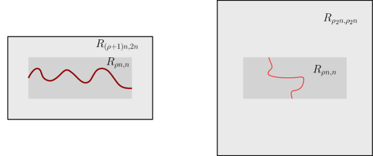
Figure 5: Theorem 9.1 (illustrated here in the case $\rho^{\prime}=\rho$, $\epsilon=1$) lower-bounds the probability of a high crossing in the difficult direction of a rectangle in a difficult domain, in terms of a polynomial of the probability for a lower crossing in the easy direction in an easy domain.

Theorem 9.1

For every $\rho,\epsilon>0$ and $\rho_{2}\geq\rho$, there exist $C=C(\rho,\rho_{2},\epsilon),c=c(\rho,\rho_{2},\epsilon)>0$ such that for all $n\geq 4/\epsilon$ and $\rho^{\prime}\leq\rho$, we have

$$c\mathbb{P}^{\pm 1}_{R_{\rho_{2}n,\rho_{2}n}}[\mathcal{V}_{\omega=1}(R_{\rho n,n})]^{C}\leq\mathbb{P}^{\pm 1}_{R_{(\rho^{\prime}+\epsilon)n,2\epsilon n}}[\mathcal{H}_{\mathcal{E}}^{*}(R_{\rho^{\prime}n,\epsilon n})],$$

where $\mathcal{E}$ denotes the set of edges with heights $h\geq 5$ at the endpoints, with additionally $B_{e}=0$ on edges $e$ between two heights $h=5$.

Remark 9.2

Note that, due to the bound on dual degree, $\mathcal{H}_{\mathcal{E}}^{*}(R_{\rho^{\prime}n,\epsilon n})\subset\mathcal{H}_{\omega=1}(R_{\rho^{\prime}n,\epsilon n})$.

We immediately record the following simple but important corollary.

Corollary 9.3

For every $\rho,\epsilon>0$ and $\rho_{2}\geq\rho$, there exists $c=c(\rho,\rho_{2},\epsilon)$ such that for all $n$, at least one of the following two holds: (i)

$$\mathbb{P}^{\pm 1}_{R_{\rho_{2}n,\rho_{2}n}}[\mathcal{H}^{*}_{\omega=0}(R_{\rho n,n})]>c;$$

or (ii) for all $\rho^{\prime}\leq\rho$, we have

$$\mathbb{P}^{\pm 1}_{R_{(\rho^{\prime}+\epsilon)n,2\epsilon n}}[\mathcal{H}_{\mathcal{E}}^{*}(R_{\rho^{\prime}n,\epsilon n})]>c.$$

Proof

Denote $\mathbb{P}^{\pm 1}_{R_{\rho_{2}n,\rho_{2}n}}[\mathcal{H}^{*}_{\omega=0}(R_{\rho n,n})]:=p_{n}$. By (6) and the above theorem,

$$\mathbb{P}^{\pm 1}_{R_{(\rho^{\prime}+\epsilon)n,2\epsilon n}}[\mathcal{H}_{\mathcal{E}}^{*}(R_{\rho^{\prime}n,\epsilon n})]\geq c^{\prime}(1-p_{n})^{C}.$$

The claim thus holds with $c=\min_{x\in[0,1]}\{x,c^{\prime}(1-x)^{C}\}$.   $\square$

The rest of the present section is dedicated to the proof of Theorem 9.1.

9.1 From vertical to horizontal crossings

We start with the key step, which creates a horizontal crossing from a vertical crossing. This step will crucially rely on treating the model on the infinite strip ${\rm Strip}(m)=\Lambda_{\infty,m}$; the horizontal shift invariance is instrumental, while the Pushing Theorem and FKG will in later subsections allow us go back to finite domains.

A boundary condition $\xi$ on a subset of ${\rm Strip}(m)$ is admissible if $\xi_{|R_{n,m}}$ is admissible on $\mathcal{H}_{R_{n,m}}$ for all $n$ (large enough). It is readily shown that there then exists a unique weak limit of $\mathbb{P}^{\xi_{|D}}_{D}$ when $D\uparrow{\rm Strip}(m)$, by the finite energy of the model, and this limit is taken as the definition of the strip measure $\mathbb{P}^{\xi}_{{\rm Strip}(m)}$. Note that the FKG and SMP properties for the strip measure (including the independent Bernoulli percolation $B$ and $\omega$ defined via $(h,B)$ as usual) directly follow from those of the finite-domain measures.

Lemma 9.4

For every $\rho>0$, there exist $C=C(\rho),c=c(\rho)>0$ such that the following holds. Let $m>n$ be integers, and let $R$ be any shifted version of the rectangle $R_{\rho n,n}$ contained in ${\rm Strip}(m)$. Then, for any $s\in\{1,3,5\}$ we have

$$c\mathbb{P}^{\{s,s+2\}}_{{\rm Strip}(m)}[\mathcal{V}^{*}_{h\omega\leq 0}(R)]^{C}\leq\mathbb{P}^{\{s,s+2\}}_{{\rm Strip}(m)}[\mathcal{H}^{*}_{h\omega\leq 0}(R)].$$

Proof

Denote $\mathbb{P}^{\{s,s+2\}}_{{\rm Strip}(m)}=:\mathbb{P}$ throughout the proof and, without loss of generality, assume that $\rho$ is an even integer and $n\geq 24$ and divisible by $3$. Subdivide $R$ into three translates of $R_{\rho n,n/3}$, denoted $R_{\mathsf{top}}$, $R_{\mathsf{mid}}$, and $R_{\mathsf{bot}}$, and overlapping in their lowest/highest row of faces, and then subdivide these top/bottom boundaries (dual-paths) into $M$ dual-vertex disjoint subsegments of width $\lfloor 2n/45\rfloor$ horizontal translational periods between endpoint faces, and overlapping at their extremal faces. Denote these subsegments by $I_{1},\ldots,I_{M}$ on the bottom-most row, then $J_{1},\ldots,J_{M}$, then $K_{1},\ldots,K_{M}$, and finally $L_{1},\ldots,L_{M}$ on the top-most row, where $M\sim 45\rho$. Define the subevents $\mathcal{V}^{i,j,k,l}(h\omega\leq 0)$, $1\leq i,j,k,l\leq M$, of $\mathcal{V}^{*}_{h\omega\leq 0}(R)$ analogously as in the Pushing theorem. Then, we define $\mathcal{V}^{i,j,k,l}_{\alpha,\beta,\gamma}(h\omega\leq 0)$ to be the event that there exists a vertical dual-crossing $\gamma^{*}$ of $R$, inducing $\mathcal{V}^{i,j,k,l}(h\omega\leq 0)$ and furthermore such that

• the unique subpath of $\gamma^{*}$ crossing $R_{\mathsf{bot}}$ passes strictly farther right than the right extreme of $I_{i-6}\cup\ldots\cup I_{i+6}$ if $\alpha=+1$ (resp. passes strictly farther left than the left extreme if $\alpha=-1$, resp. remains right above them if $\alpha=0$); and

• the unique subpath of $\gamma^{*}$ crossing $R_{\mathsf{top}}$ passes strictly farther right than the right extreme of $L_{l-6}\cup\ldots\cup L_{l+6}$ if $\gamma=+1$ (resp. passes strictly farther left that the left extreme if $\gamma=-1$, resp. remains right above them if $\gamma=0$); and

• the related subcurve $\eta^{*}$ of $\gamma^{*}$ passes strictly farther right than the right extreme of $J_{i-6}\cup\ldots\cup J_{i+6}$ if $\beta=+1$ (resp. passes strictly farther left that the left extreme if $\beta=-1$, resp. remains right above them if $\beta=0$).

By the Union bound, there exists $(i_{0},j_{0},k_{0},l_{0},\alpha_{0},\beta_{0},\gamma_{0})$ such that

$$\mathbb{P}[\mathcal{V}^{i_{0},j_{0},k_{0},l_{0}}_{\alpha_{0},\beta_{0},\gamma_{0}}(h\omega\leq 0)]\geq\tfrac{1}{N}\mathbb{P}[\mathcal{V}^{*}_{h\omega\leq 0}(R)],$$ (13)

where $N=M^{4}\cdot 3^{3}$ is the total number of tuples $(i,j,k,l,\alpha,\beta,\gamma)$. Let $\mathcal{E}^{*}_{h\omega\leq 0}(\ell)$ denote the horizontal shift of the event $\mathcal{V}^{i_{0},j_{0},k_{0},l_{0}}_{\alpha_{0},\beta_{0},\gamma_{0}}(h\omega\leq 0)$, so that the related crossing lands on $I_{\ell}$ on the bottom, instead of $I_{i_{0}}$. Note that the events $\mathcal{E}^{*}_{h\omega\leq 0}(\ell)$ are decreasing in $(h,B)$. By the shift symmetry and FKG,

$$\mathbb{P}[\bigcap_{\begin{subarray}{c}\ell=2\\ \ell\text{ even}\end{subarray}}^{8}\mathcal{E}^{*}_{h\omega\leq 0}(\ell)]\geq\left(\mathbb{P}[\mathcal{V}^{i_{0},j_{0},k_{0},l_{0}}_{\alpha_{0},\beta_{0},\gamma_{0}}(h\omega\leq 0)]\right)^{4}.$$ (14)

Let now $\mathcal{B}^{*}_{h\omega\leq 0}(\ell)$ be the “bridge event” that there is a dual crossing of $h\omega\leq 0$ in the horizontal strip of $R$ (i.e., the union of all horizontal shifts of $R$), from the semi-infinite line on left of $I_{\ell}$ to the semi-infinite line on the right. If for any $\ell_{0}\in\{3,5,7\}$,

$$\mathbb{P}[\mathcal{B}^{*}_{h\omega\leq 0}(\ell_{0})\;|\;\bigcap_{\begin{subarray}{c}\ell=2\\ \ell\text{ even}\end{subarray}}^{8}\mathcal{E}^{*}_{h\omega\leq 0}(\ell)]\geq 1/3,$$ (15)

then the proof is trivially finished by computing

$$\mathbb{P}[\mathcal{H}^{*}_{h\omega\leq 0}(R)]\geq\mathbb{P}[\bigcap_{\ell=1}^{M}\mathcal{B}^{*}_{h\omega\leq 0}(\ell)]\geq\mathbb{P}[\mathcal{B}_{h\omega\leq 0}^{*}(\ell_{0})]^{M},$$ (16)

where the first step was an inclusion of events and the second one relied on shift invariance and FKG. Now, combining (13)–(16), we obtain the claim.

For the rest of the proof, we thus assume that (15) does not hold true; hence

$$\mathbb{P}[\mathcal{B}^{*}_{h\omega\leq 0}(3)^{c}\cap\mathcal{B}^{*}_{h\omega\leq 0}(7)^{c}\;|\;\bigcap_{\begin{subarray}{c}\ell=2\\ \ell\text{ even}\end{subarray}}^{8}\mathcal{E}^{*}_{h\omega\leq 0}(\ell)]\geq 1/3.$$ (17)

Let now $\tilde{h}=6-h$, and define $\nu$ on $E$ by (10). Recall from the Pushing theorem the idea that $\omega=0\Rightarrow\nu=0$, but $\nu$ has been modified from $\omega$ to remove information about $\mathrm{sign}(\tilde{h})$. Define the event $\mathcal{W}^{i,j,k,l}_{\alpha,\beta,\gamma}(\nu=0)$ that there exists a vertical dual-crossing $\gamma^{*}$ of the horizontal strip of $R$, with $\nu=0$ and furthermore such that

• the unique subpath of $\gamma^{*}$ crossing the strip of $R_{\mathsf{bot}}$ lands on $I_{i-1}\cup I_{i}\cup I_{i+1}$ on the bottom and, if $\alpha=+1$ (resp. $\alpha=-1$, resp. $\alpha=0$), it passes strictly farther right than the right extreme of $I_{i+5}$ (resp. passes strictly farther left that the left extreme of $I_{i-5}$, resp. remains right above $I_{i-7}\cup\ldots\cup I_{i+7}$); and

• the unique subpath of $\gamma^{*}$ crossing the strip of $R_{\mathsf{top}}$ vertically lands on $L_{l-1}\cup L_{l}\cup L_{l+1}$ on the top and, if $\gamma=+1$ (resp. $\gamma=-1$, resp. $\gamma=0$), passes strictly farther right than the right extreme of $L_{l+5}$ (resp. passes strictly farther left that the left extreme of $L_{l-5}$, resp. remains right below $L_{l-7}\cup\ldots\cup L_{l+7}$); and

• the related $\eta^{*}$ (the first crossing of the strip of $R_{\mathsf{mid}}$) traverses between $J_{j-1}\cup J_{j}\cup J_{j+1}$ and $K_{k-1}\cup K_{k}\cup K_{k+1}$ and, if $\beta=+1$ (resp. $\beta=-1$, resp. $\beta=0$), passes strictly farther right than the right extreme $J_{j+5}$ (resp. passes strictly farther left that the left extreme of $J_{j-5}$, resp. remains right above $J_{i-7}\cup\ldots\cup J_{i+7}$).

Lemma 9.5

Suppose that $\mathcal{E}^{*}_{h\omega\leq 0}(2)\cap\mathcal{B}^{*}_{h\omega\leq 0}(3)^{c}\cap\mathcal{E}^{*}_{h\omega\leq 0}(4)$ occurs. Then, there exists a vertical dual-crossing of the strip of $R$ with $\nu=0$ that lands on $I_{i_{0}+x}\cup I_{i_{0}+x+1}$ on the bottom and on $L_{l_{0}+x}\cup L_{l_{0}+x+x}$ on the top, where $x=3-i_{0}$. Furthermore, the left-most such dual-crossing induces the event $\mathcal{W}^{i_{0}+x,j_{0}+x,k_{0}+x,l_{0}+x\;*}_{\alpha_{0},\beta_{0},\gamma_{0}}(\nu=0)$.

The proof is essentially identical to that of Lemma 8.8 (indeed $\mathcal{E}^{*}_{h\omega\leq 0}(2)\cap\mathcal{B}^{*}_{h\omega\leq 0}(3)^{c}\cap\mathcal{E}^{*}_{h\omega\leq 0}(4)$ means that there is a primal crossing of $h\omega\geq 1$ from $I_{3}$ to the top of the rectangle of $R$, and this primal crossing cannot cross any dual-crossing generating $\mathcal{E}^{*}_{h\omega\leq 0}(2)$ or $\mathcal{E}^{*}_{h\omega\leq 0}(4)$.). The obvious analogue of this lemma holds on the event $\mathcal{E}^{*}_{h\omega\leq 0}(6)\cap\mathcal{B}^{*}_{h\omega\leq 0}(7)^{c}\cap\mathcal{E}^{*}_{h\omega\leq 0}(8)$, with “left” and “right” reversed and $x=7-i_{0}$. Let $\gamma^{*}_{\mathsf{left}}$ (resp. $\gamma^{*}_{\mathsf{right}}$) be such left-most (resp. right-most) vertical dual-crossings; on $\mathcal{B}^{*}_{h\omega\leq 0}(3)^{c}\cap\mathcal{B}^{*}_{h\omega\leq 0}(7)^{c}\bigcap_{\begin{subarray}{c}\ell=2\\ \ell\text{ even}\end{subarray}}^{8}\mathcal{E}^{*}_{h\omega\leq 0}(\ell)$ they exist. In that case, let $\mathcal{X}$ be the quad bounded by $\gamma^{*}_{\mathsf{left}}$, $\gamma^{*}_{\mathsf{right}}$, and the top and bottom boundary segments of the strip of $R$ between them. Let $\Xi$ be the collection of all such sub-quads of this strip, whose left (resp. right) side both is of the type $\mathcal{W}^{i_{0}+x,j_{0}+x,k_{0}+x,l_{0}+x\;*}_{\alpha_{0},\beta_{0},\gamma_{0}}(\nu=0)$ with $x=3-i_{0}$ (resp. $x=7-i_{0}$). The previous lemma yields

$$\bigg{\{}\mathcal{B}^{*}_{h\omega\leq 0}(3)^{c}\cap\mathcal{B}^{*}_{h\omega\leq 0}(7)^{c}\bigcap_{\begin{subarray}{c}\ell=2\\ \ell\text{ even}\end{subarray}}^{8}\mathcal{E}^{*}_{h\omega\leq 0}(\ell)\bigg{\}}\subset\{\mathcal{X}\in\Xi\},$$

so combined with (17), we obtain

$$\mathbb{P}[\mathcal{X}\in\Xi]\geq\tfrac{1}{3}\mathbb{P}[\bigcap_{\begin{subarray}{c}\ell=2\\ \ell\text{ even}\end{subarray}}^{8}\mathcal{E}^{*}_{h\omega\leq 0}(\ell)].$$ (18)

To conclude the proof,one then shows identically to Lemma 8.9 that

$$\mathbb{P}[\mathcal{V}_{h\omega\geq 1}(X)\;|\;\mathcal{X}=X]\leq\tfrac{31}{32},\qquad\text{for any }X\in\Xi,$$

and noticing that $\mathcal{V}_{h\omega\geq 1}(X)^{c}=\mathcal{H}_{h\omega\leq 0}^{*}(X)\subset\mathcal{B}^{*}_{h\omega\leq 0}(5)$ (on the event $\mathcal{X}=X$), one deduces

$$\mathbb{P}[\mathcal{B}^{*}_{h\omega\leq 0}(5)]\geq\tfrac{1}{32}\mathbb{P}[\mathcal{X}\in\Xi].$$ (19)

Finally, combining inequalities (13)–(14), (18)–(19) and in the end (16), we obtain the claimed inequality under the assumption (17). This completes the proof.   $\square$

9.2 Increasing the height on the crossings

The next step is to increase the height on the horizontal crossing. The price to pay for this increase is an increase in the size of the domain, which will be handled in later subsections.

Proposition 9.6

For every $\rho>0$ and $\rho_{2}\geq 3$, there exist $C=C(\rho,\rho_{2}),c=c(\rho,\rho_{2})>0$ and $\rho_{3}=\rho_{3}(\rho,\rho_{2})\in\mathbb{Z}_{+}$ such that for all $n\in\mathbb{N}$, we have

$$c\mathbb{P}_{R_{\rho_{2}n,\rho_{2}n}}^{\pm 1}[\mathcal{V}_{\omega=1}(R_{\rho n,n})]^{C}\leq\mathbb{P}_{{\rm Strip}(\rho_{3}n)}^{\pm 1}[\mathcal{H}^{*}_{\mathcal{E}}(R_{\rho n,n})],$$

where the random edge set $\mathcal{E}$ is defined as in Theorem 9.1.

We work towards this proposition in several steps. In the following, for $0<s\in\mathbb{Z}_{\mathrm{odd}}$, let $\{h\geq_{B}s\}$ denote the random set of edges on which $h\geq s$ and additionally for an edge $e$ between two heights $s$, $B_{e}=1$; and let $\mathcal{E}_{s}=\mathcal{E}_{s}(h,B)$ denote the set of edges with heights $h\geq s$ at the endpoints, with additionally $B_{e}=0$ on edges $e$ between two heights $h=s$. (Hence $\{h\geq_{B}1\}=\{h\omega\geq 1\}$ and the set $\mathcal{E}$ in Theorem 9.1 coincides with $\mathcal{E}_{5}$.) For two rectangles $R\subset R^{\prime}$, denote by $\mathcal{O}^{*}_{\mathcal{E}_{s}}(R,R^{\prime})$ the event that there is a dual-loop in $R^{\prime}$, on the dual-edges $\mathcal{E}_{s}^{*}$, that surrounds $R$. We now have the following (see Figure 6 (left)):

    

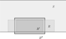
Figure 6: Two simple illustrations on RSW results. Left: Lemma 9.4 tells one how to “construct horizontal crossings from vertical ones”. A step in the proof of Lemma 9.7 is to similarly “construct loops”. Right: The geometric setup in the proof of Proposition 9.10.

Lemma 9.7

For every $\rho>0$ and $\rho_{2}\geq 3$, there exist $C=C(\rho,\rho_{2}),c=c(\rho,\rho_{2})>0$ such that the following holds. Let $n\in\mathbb{N}$ and $(R,R^{\prime},S)$ be a translate of the triplet $(R_{\rho n,n},R_{3\rho n,3n},{\rm Strip}(\rho_{2}n))$, and let $m$ be large enough so that $S\subset{\rm Strip}(m)$. Then, for any $s\in\{1,3,5\}$, we have

$$c\mathbb{P}_{{\rm Strip}(\rho_{2}n)}^{\pm 1}[\mathcal{V}_{h\geq_{B}s}(R_{\rho n,3n})]^{C}\leq\mathbb{P}_{{\rm Strip}(m)}^{\pm 1}[\mathcal{O}^{*}_{\mathcal{E}_{s}}(R,R^{\prime})].$$

Proof

Denote $\mathbb{P}_{{\rm Strip}(\rho_{2}n)}^{\pm 1}:=\mathbb{P}_{1}$ and $\mathbb{P}_{{\rm Strip}(m)}^{\pm 1}=:\mathbb{P}_{2}$. Denote by $\{|h|\geq_{B}s\}$ the edges on which $|h|\geq s$ and additionally $B=1$ between two absolute-heights $|h|=s$. Note that this edge set is increasing in $(|h|,B)$, and that the sign of $h$ is fixed on any cluster of $\{|h|\geq_{B}s\}$. Subdivide $R^{\prime}$ into three translates $R_{1},R_{2},R_{3}$ of $R_{\rho n,3n}$, indexed from left to right. By sign flip symmetry, then FKG and finally inclusion, we have for all $1\leq i\leq 3$

$$\mathbb{P}_{2}[\mathcal{V}_{h\geq_{B}s}(R_{i})]\geq\tfrac{1}{2}\mathbb{P}_{2}[\mathcal{V}_{|h|\geq_{B}s}(R_{i})]\geq\tfrac{1}{2}\mathbb{P}_{1}[\mathcal{V}_{|h|\geq_{B}s}(R_{\rho n,3n})]\geq\tfrac{1}{2}\mathbb{P}_{1}[\mathcal{V}_{h\geq_{B}s}(R_{\rho n,3n})].$$

Next, let $\tilde{B}$ be equally distributed with $B$ and coupled so that $B_{e}=1\Rightarrow\tilde{B}_{e}=0$. In this coupling, $\{h\geq_{B}s\}\subset\mathcal{E}_{s}(h,\tilde{B})$. Combining this observation with (7),

$$\mathbb{P}_{2}[\mathcal{V}_{h\geq_{B}s}(R_{i})]\leq\mathbb{P}_{2}[\mathcal{V}^{*}_{\mathcal{E}_{s}(h,\tilde{B})}(R_{i})]=\mathbb{P}_{2}[\mathcal{V}^{*}_{\mathcal{E}_{s}}(R_{i})].$$

Then subdivide $R^{\prime}$ into three translates $R_{4},R_{5},R_{6}$ of $R_{3\rho n,n}$, indexed from bottom to top. By Lemma 9.4, we have for all $4\leq i\leq 6$

$$\mathbb{P}_{2}[\mathcal{H}^{*}_{\mathcal{E}_{s}}(R_{i})]\geq c^{\prime}\mathbb{P}_{2}[\mathcal{V}^{*}_{\mathcal{E}_{s}}(R_{i})]^{C^{\prime}}$$

for suitable $C^{\prime}=C^{\prime}(\rho),c^{\prime}=c^{\prime}(\rho)>0$, and by inclusion

$$\mathbb{P}_{2}[\mathcal{V}^{*}_{\mathcal{E}_{s}}(R_{i})]\geq\mathbb{P}_{2}[\mathcal{V}^{*}_{\mathcal{E}_{s}}(R_{2})].$$

Finally, by inclusion and FKG for $(h,-B)$,

$$\mathbb{P}_{2}[\mathcal{O}^{*}_{\mathcal{E}_{s}}(R,R^{\prime})] \geq\mathbb{P}_{2}[\mathcal{V}^{*}_{\mathcal{E}_{s}}(R_{1})\cap\mathcal{V}^{*}_{\mathcal{E}_{s}}(R_{3})\cap\mathcal{H}^{*}_{\mathcal{E}_{s}}(R_{4})\cap\mathcal{H}^{*}_{\mathcal{E}_{s}}(R_{6})]$$

$$\geq\mathbb{P}_{2}[\mathcal{V}^{*}_{\mathcal{E}_{s}}(R_{1})]\mathbb{P}_{2}[\mathcal{V}^{*}_{\mathcal{E}_{s}}(R_{3})]\mathbb{P}_{2}[\mathcal{H}^{*}_{\mathcal{E}_{s}}(R_{4})]\mathbb{P}_{2}[\mathcal{H}^{*}_{\mathcal{E}_{s}}(R_{6})].$$

The claim now follows by combining all the displayed inequalities.   $\square$

Lemma 9.8

For every $\rho\leq\rho_{2}$ and $s\in\{1,3,5\}$, there exist $C=C(\rho,\rho_{2},s),c=c(\rho,\rho_{2},s)>0$ and $\rho_{3}=\rho_{3}(\rho,\rho_{2},s)\in\mathbb{Z}_{+}$ such that, for all $n\in\mathbb{N}$, we have

$$c\mathbb{P}_{R_{\rho_{2}n,\rho_{2}n}}^{\pm 1}[\mathcal{V}_{\omega=1}(R_{\rho n,n})]^{C}\leq\mathbb{P}_{{\rm Strip}(\rho_{3}n)}^{\pm 1}[\mathcal{V}_{h\geq_{B}s}(R_{\rho n,n})].$$

Proof

The proof is an induction on $s$. In the base case $s=1$, by FKG and sign flip symmetry,

$$\mathbb{P}_{R_{\rho_{2}n,\rho_{2}n}}^{\pm 1}[\mathcal{V}_{\omega=1}(R_{\rho n,n})]\leq\mathbb{P}_{{\rm Strip}(\rho_{2}n)}^{\pm 1}[\mathcal{V}_{\omega=1}(R_{\rho n,n})]\leq 2\mathbb{P}_{{\rm Strip}(\rho_{2}n)}^{\pm 1}[\mathcal{V}_{h\omega\geq 1}(R_{\rho n,n})].$$

Recalling that $\{h\omega\geq 1\}=\{h\geq_{B}1\}$, this proves the base case, with $\rho_{3}=\rho_{2}$.

Assume that the claim holds for $s\in\{1,3\}$, i.e., there exist $C(s),c(s),\rho_{3}(s)$ (we omit $\rho,\rho_{2}$ for lighter notation) such that

$$c(s)\mathbb{P}_{R_{\rho_{2}n,\rho_{2}n}}^{\pm 1}[\mathcal{V}_{\omega=1}(R_{\rho n,n})]^{C(s)}\leq\mathbb{P}_{{\rm Strip}(\rho_{3}(s)n)}^{\pm 1}[\mathcal{V}_{h\geq_{B}s}(R_{\rho n,n})],$$ (20)

and aim to prove it for $s+2$. Denote $(R,R^{\prime},R^{\prime\prime})=:(R_{\rho n,n},R_{\rho_{2}n,\rho_{2}n},2R_{\rho_{2}n,\rho_{2}n})$ for short; by Lemma 9.7 and a standard necklace argument, for any $\rho_{3}(s+2)$ large enough (fix any for definiteness),

$$\mathbb{P}_{{\rm Strip}(\rho_{3}(s+2)n)}^{\pm 1}[\mathcal{O}_{\mathcal{E}_{s}}^{*}(R^{\prime},R^{\prime\prime})]\geq c^{\prime}\mathbb{P}_{{\rm Strip}(\rho_{3}(s)n)}^{\pm 1}[\mathcal{V}_{h\geq_{B}s}(R_{\rho n,n})]^{C^{\prime}}.$$ (21)

for suitable $c^{\prime},C^{\prime}>0$ depending on $\rho$ and $\rho_{3}(s)$.

Next, let $h\sim\mathbb{P}_{{\rm Strip}(\rho_{3}(s+2)n)}^{\pm 1}$, and define $\tilde{h}=s+1-h$ and $\tilde{\omega}$ based on $(\tilde{h},B)$ as usual. Note that $\mathcal{E}_{s}(h,B)=\{\tilde{h}\tilde{\omega}\leq 0\}$. On the event $\mathcal{O}_{\mathcal{E}_{s}}^{*}(R^{\prime},R^{\prime\prime})$, explore the primal-component of $\tilde{h}\tilde{\omega}\geq 1$ starting from $\partial R^{\prime\prime}$ and its bounding dual curves of $\tilde{h}\tilde{\omega}\leq 0$. Let $X$ be the unique unexplored component that contains $R^{\prime}$ (a simply-connected domain bounded by a dual curve); by the SMP, the exploration generates, in terms of $\tilde{h}$, a boundary condition $\tilde{\xi}\preceq\{\pm 1\}$ on $\partial X$ (in terms of $h$, $\xi=2-\tilde{\xi}\succeq\{s,s+2\}$). Now, compute

$$\mathbb{P}^{\xi}_{X}[\mathcal{V}_{h\geq_{B}s+2}(R)] \geq\mathbb{P}^{\{s,s+2\}}_{X}[\mathcal{V}_{h\geq_{B}s+2}(R)]\qquad\text{(by CBC for $(h,B)$)}$$

$$=\mathbb{P}^{\pm 1}_{X}[\mathcal{V}_{h\omega\geq 1}(R)]\qquad\text{(by height shift)}$$

$$\geq\tfrac{1}{2}\mathbb{P}^{\pm 1}_{X}[\mathcal{V}_{\omega=1}(R)]\qquad\text{(by sign flip symmetry)}$$

$$\geq\tfrac{1}{2}\mathbb{P}^{\pm 1}_{R^{\prime}}[\mathcal{V}_{\omega=1}(R)]\qquad\text{(by FKG for $(|h|,\omega)$).}$$

Averaging over $X$, one obtains

$$\mathbb{P}_{{\rm Strip}(\rho_{3}(s+2)n)}^{\pm 1}[\mathcal{V}_{h\geq_{B}s+2}(R)\;|\;\mathcal{O}_{\mathcal{E}_{s}}^{*}(R^{\prime},R^{\prime\prime})]\geq\tfrac{1}{2}\mathbb{P}^{\pm 1}_{R^{\prime}}[\mathcal{V}_{\omega=1}(R)].$$ (22)

Combining (20)–(22), the claim also holds for $s+2$. This concludes the proof.   $\square$

Proof of Proposition 9.6

By the previous lemma (case $s=5$), there exist $C^{\prime}=C^{\prime}(\rho,\rho_{2}),c^{\prime}=c^{\prime}(\rho,\rho_{2})>0$ and $\rho_{3}=\rho_{3}(\rho,\rho_{2})\in\mathbb{Z}_{+}$ such that

$$c^{\prime}\mathbb{P}_{R_{\rho_{2}n,\rho_{2}n}}^{\pm 1}[\mathcal{V}_{\omega=1}(R_{\rho n,n})]^{C^{\prime}}\leq\mathbb{P}_{{\rm Strip}(\rho_{3}n)}^{\pm 1}[\mathcal{V}_{h\geq_{B}5}(R_{\rho n,n})].$$

Letting again $\tilde{B}$ be equally distributed with $B$ and coupled so that $B_{e}=1\Rightarrow\tilde{B}_{e}=0$; note that $\{h\geq_{B}5\}\subset\mathcal{E}_{5}(h,\tilde{B})=\mathcal{E}(h,\tilde{B})$. Combining with (7),

$$\mathbb{P}_{{\rm Strip}(\rho_{3}n)}^{\pm 1}[\mathcal{V}_{h\geq_{B}5}(R_{\rho n,n})]\leq\mathbb{P}_{{\rm Strip}(\rho_{3}n)}^{\pm 1}[\mathcal{V}_{\mathcal{E}}^{*}(R_{\rho n,n})].$$

Finally, by Lemma 9.4, there exist $C^{\prime\prime}=C^{\prime\prime}(\rho),c^{\prime\prime}=c^{\prime\prime}(\rho)>0$ such that

$$c^{\prime\prime}\mathbb{P}_{{\rm Strip}(\rho_{3}n)}^{\pm 1}[\mathcal{V}_{\mathcal{E}}^{*}(R_{\rho n,n})]^{C^{\prime\prime}}\leq\mathbb{P}_{{\rm Strip}(\rho_{3}n)}^{\pm 1}[\mathcal{H}_{\mathcal{E}}^{*}(R_{\rho n,n})].$$

Combining the three above displayed inequalities concludes the proof.   $\square$

9.3 Pushing the crossings

In the next two subsections, we give two lemmas: one to “push a horizontal crossing downwards”, and another to “push the top boundary downwards”. An iterated use of these lemmas will compensate the increase in domain size that appeared in Proposition 9.6.

Lemma 9.9

For every $\rho>0$, there exist constants $C=C(\rho),c=c(\rho)>0$ such that the following holds for any $n$. Let $R=R_{\rho n,9n}$ and let $R^{\prime}$ be a translate of the rectangle $R_{\rho n,7n}$ so that it lies on the bottom of ${\rm Strip}(11n)$. Then, we have

$$\mathbb{P}^{\pm 1}_{{\rm Strip}(11n)}[\mathcal{H}_{\mathcal{E}}^{*}(R^{\prime})]\geq c\mathbb{P}^{\pm 1}_{{\rm Strip}(11n)}[\mathcal{H}_{\mathcal{E}}^{*}(R)]^{C}.$$

Proof

Let us denote $\mathbb{P}^{\pm 1}_{{\rm Strip}(11n)}=:\mathbb{P}$. Let $R_{\mathsf{top}}$, $R_{\mathsf{mid}}$, and $R_{\mathsf{bot}}$ denote the top, middle and bottom thirds of the rectangle $R$. Let $\mathcal{H}^{\mathsf{tm}}$ (resp. $\mathcal{H}^{\mathsf{mb}}$, resp. $\mathcal{H}^{\mathsf{all}}$) be the subevent of $\mathcal{H}_{\mathcal{E}}^{*}(R)$ that there is a horizontal $\mathcal{E}^{*}$ dual-crossing of $R$ that is contained in $R_{\mathsf{top}}\cup R_{\mathsf{mid}}$ (resp. contained in $R_{\mathsf{mid}}\cup R_{\mathsf{bot}}$, resp. visits all three sub-rectangles). By the Union Bound,

$$\mathbb{P}[\mathcal{H}_{\mathcal{E}}^{*}(R)]\leq\mathbb{P}[\mathcal{H}^{\mathsf{tm}}]+\mathbb{P}[\mathcal{H}^{\mathsf{mb}}]+\mathbb{P}[\mathcal{H}^{\mathsf{all}}],$$

so at least one of the events on the right-hand side has a probability larger or equal to $\tfrac{1}{3}\mathbb{P}[\mathcal{H}_{\mathcal{E}}^{*}(R)]$. If $\mathcal{H}^{\mathsf{all}}$ is not such an event, then by symmetry, $\mathcal{H}^{\mathsf{mb}}$ is one, and with an inclusion of events, we deduce

$$\mathbb{P}[\mathcal{H}_{\mathcal{E}}^{*}(R^{\prime})]\geq\mathbb{P}[\mathcal{H}^{\mathsf{mb}}]\geq\tfrac{1}{3}\mathbb{P}[\mathcal{H}_{\mathcal{E}}^{*}(R)],$$

which proves the claim. If, $\mathcal{H}^{\mathsf{all}}$ is such an event then we infer by inclusion of events that

$$\mathbb{P}[\mathcal{V}^{*}_{\mathcal{E}}(R^{\mathsf{mid}})]\geq\mathbb{P}[\mathcal{H}^{\mathsf{all}}]\geq\tfrac{1}{3}\mathbb{P}[\mathcal{H}_{\mathcal{E}}^{*}(R)],$$

and by another inclusion of events and Lemma 9.4 that

$$\mathbb{P}[\mathcal{H}_{\mathcal{E}}^{*}(R^{\prime})]\geq\mathbb{P}[\mathcal{H}_{\mathcal{E}}^{*}(R^{\mathsf{mid}})]\geq c^{\prime}\mathbb{P}[\mathcal{V}^{*}_{\mathcal{E}}(R^{\mathsf{mid}})]^{C^{\prime}},$$

for suitable $C^{\prime}=C^{\prime}(\rho),c^{\prime}=c^{\prime}(\rho)>0$. This concludes the proof.   $\square$

9.4 Pushing the boundaries

Proposition 9.10

For every $\rho,\epsilon>0$ and $\rho_{2}\geq 1$, there exists $c=c(\rho,\rho_{2},\epsilon)>0$ such that the following holds for any $n\geq 4/\epsilon$. Let $R$ be a translate of the rectangle $R_{\rho n,n}$ on the bottom of ${\rm Strip}(\rho_{2}n)$, let $w\leq\rho n$ and $R^{\prime}:=R_{w,n}$ and $R^{\prime\prime}=R_{w+\epsilon n,(1+\epsilon)n}$. Then, we have

$$c\mathbb{P}^{\pm 1}_{{\rm Strip}(\rho_{2}n)}[\mathcal{H}_{\mathcal{E}}^{*}(R)]\leq\mathbb{P}^{\pm 1}_{R^{\prime\prime}}[\mathcal{H}_{\mathcal{E}}^{*}(R^{\prime})].$$

The rest of this subsection constitutes the proof of this result. Throughout the subsection, denote ${\rm Strip}(\rho_{2}n)=:S$ and assume that $R^{\prime}$ and $R^{\prime\prime}$ are shifted so that $R^{\prime}$ is still in the middle of $R^{\prime\prime}$ and that $R^{\prime}$ lies inside $R$ (Figure 6 (right)). Let $\mathcal{E}^{\prime}$ denote the set of edges between absolute-heights $|h|\geq 5$, with additionally $B=0$ on edges between two absolute-heights $|h|=5$. Let $\mathcal{U}$ be the event that there is a horizontal dual-crossing of $R^{\prime}$ on the dual-edges crossing $\mathcal{E}^{\prime}$, i.e., generating $\mathcal{H}_{\mathcal{E}^{\prime}}^{*}(R^{\prime})$, whose component of $\omega=1$ (indeed, by the bound on the dual degree, the primal-edges crossed by such a dual-path are contained in a single component of $\omega=1$) is furthermore disconnected from the top and side boundaries of $R^{\prime\prime}$ (hence by some dual-path of $\omega=0$).

Lemma 9.11

In the setup and notation given above, we have

$$\mathbb{P}^{\pm 1}_{S}[\mathcal{U}]\leq\mathbb{P}^{\pm 1}_{R^{\prime\prime}}[\mathcal{H}_{\mathcal{E}^{\prime}}^{*}(R^{\prime})].$$ (23)

Proof

Explore the primal clusters of $\omega=1$ in $R^{\prime\prime}\cap S$ that are adjacent to the top and side boundaries of $R^{\prime\prime}$, and the dual curves of $\omega=0$ bounding them. Let $\mathcal{X}\subset R^{\prime\prime}\cap S$ be the random set edges where $\omega$ is explored; the event $\mathcal{X}=X$ can thus be inferred from $\omega_{|X}$. Let $\Xi(X)$ be the set of such $\alpha$ that $\omega_{|X}=\alpha$ generates the event $\mathcal{X}=X$, so

$$\mathbb{P}^{\pm 1}_{S}[\mathcal{U}\cap\{\mathcal{X}=X\}]=\sum_{\alpha\in\Xi(X)}\mathbb{P}^{\pm 1}_{S}[\omega_{|X}=\alpha]\mathbb{P}^{\pm 1}_{S}[\mathcal{H}^{*}_{\mathcal{E}^{\prime}\cap X^{c}}(R^{\prime})\;|\;\omega_{|X}=\alpha].$$

Now, by the SMP, the event $\omega_{|X}=\alpha$ generates a boundary condition $\{\pm 1\}$ for the unexplored components, the height configurations in the single individual components being independent, and this law for heights on $X^{c}$ is also obtained by setting $\omega_{|X}=0$. Compute

$$\mathbb{P}^{\pm 1}_{S}[\mathcal{H}^{*}_{\mathcal{E}^{\prime}\cap X^{c}}(R^{\prime})\;|\;\omega_{|X}=\alpha] =\mathbb{P}^{\pm 1}_{S}[\mathcal{H}^{*}_{\mathcal{E}^{\prime}\cap X^{c}}(R^{\prime})\;|\;\omega_{|X}=0]\qquad\text{(by SMP)}$$

$$=\mathbb{P}^{\pm 1}_{R^{\prime\prime}}[\mathcal{H}^{*}_{\mathcal{E}^{\prime}\cap X^{c}}(R^{\prime})\;|\;\omega_{|X}=0]\qquad\text{(by SMP)}$$

$$\leq\mathbb{P}^{\pm 1}_{R^{\prime\prime}}[\mathcal{H}^{*}_{\mathcal{E}^{\prime}\cap X^{c}}(R^{\prime})]\qquad\text{(by FKG for $(|h|,-B)$)}$$

$$\leq\mathbb{P}^{\pm 1}_{R^{\prime\prime}}[\mathcal{H}^{*}_{\mathcal{E}^{\prime}}(R^{\prime})]\qquad\text{(by inclusion).}$$

Combining the two previously displayed equations yields

$$\mathbb{P}^{\pm 1}_{S}[\mathcal{U}\cap\{\mathcal{X}=X\}]\leq\mathbb{P}^{\pm 1}_{S}[\mathcal{X}=X]\mathbb{P}^{\pm 1}_{R^{\prime\prime}}[\mathcal{H}_{\mathcal{E}^{\prime}}^{*}(R^{\prime})],$$

and summing this over all possible values of $X$ gives (23).   $\square$

Lemma 9.12

In the setup and notation given in Proposition 9.10 and right below it, there exists $c^{\prime}=c^{\prime}(\rho,\rho_{2},\epsilon)>0$ such that

$$\mathbb{P}^{\pm 1}_{S}[\mathcal{U}]\geq c^{\prime}\mathbb{P}^{\pm 1}_{S}[\mathcal{H}_{\mathcal{E}^{\prime}}^{*}(R)].$$ (24)

Proof

Set

$$\nu_{\langle u,v\rangle}=\begin{cases}0,\qquad\{|{h}(u)|,|{h}(v)|\}=\{5,7\}\\ B_{\langle u,v\rangle},\qquad|{h}(u)|=|{h}(v)|\in\{5,7\}\\ 1,\qquad\text{otherwise}\end{cases}$$

and note that under the boundary condition $\mathbb{P}^{\{\pm 1\}}_{S}=:\mathbb{P}$, $\mathcal{H}_{\mathcal{E}^{\prime}}^{*}(R^{\prime})=\mathcal{H}_{\nu=0}^{*}(R^{\prime})$. Thus, explore the primal-cluster of $\nu=1$ in $R^{\prime}$ that is adjacent to the bottom of $R^{\prime}$, and the primal curves of $\nu=0$ bounding it; this reveals the lowest crossing inducing $\mathcal{H}_{\nu=0}^{*}(R^{\prime})$ (if such exists). Let us also explore $h$ on the primal-clusters, hence in $[-5,5]$. Let $\mathcal{Y}=(V(\mathcal{Y}),E(\mathcal{Y}))$ be the set where $h$ and $\nu$ are thus explored; the event $\mathcal{Y}=Y$ can be inferred from $\nu_{|Y}$; let $\Psi$ be the set of $(Y,\chi,\beta)$ such that $\{h_{|Y}=\chi,\nu_{|Y}=\beta\}$ induces $\mathcal{Y}=Y$ and $\mathcal{H}_{\nu=0}^{*}(R^{\prime})$, so

$$\mathbb{P}[\mathcal{H}_{\nu=0}^{*}(R^{\prime})]=\sum_{(Y,\chi,\beta)\in\Psi}\mathbb{P}[h_{|Y}=\chi,\nu_{|Y}=\beta]$$

and

$$\mathbb{P}[\mathcal{U}]=\mathbb{P}[\mathcal{U}\cap\mathcal{H}_{\nu=0}^{*}(R^{\prime})]=\sum_{(Y,\chi,\beta)\in\Psi}\mathbb{P}[h_{|Y}=\chi,\nu_{|Y}=\beta]\mathbb{P}[\mathcal{U}\;|\;h_{|Y}=\chi,\nu_{|Y}=\beta]$$

Note also that on the unique $\mathcal{H}_{\nu=0}^{*}(R^{\prime})$ crossing found in $\beta$, the sign of $\chi$ is constant (due to the bound on dual degree); let us assume it is $+1$ for definiteness (without loss of generality, due to sign flip symmetry). Then, given $\{h_{|Y}=\chi,\nu_{|Y}=\beta\}$, $\mathcal{U}$ happens at least if there is a dual path (“bridge”) of $h\omega\leq 0$ in $(R^{\prime\prime}\cap S)\setminus Y$, that disconnects the the bottom of the smaller rectangle $R^{\prime}$ from the top, left, and right sides of the bigger rectangle $R^{\prime\prime}\cap S$. We denote this event by $\mathcal{B}_{h\omega\leq 0}^{*}(Y)$; then, in equations

$$\mathbb{P}[\mathcal{U}\;|\;h_{|Y}=\chi,\nu_{|Y}=\beta]\geq\mathbb{P}[\mathcal{B}_{h\omega\leq 0}^{*}(Y)\;|\;h_{|Y}=\chi,\nu_{|Y}=\beta]$$

We will show below that there exists $c^{\prime}=c^{\prime}(\rho,\rho_{2},\epsilon)$ such that, for any $(Y,\chi,\beta)\in\Psi$,

$$\mathbb{P}[\mathcal{B}_{h\omega\leq 0}^{*}(Y)\;|\;h_{|Y}=\chi,\nu_{|Y}=\beta]\geq c^{\prime}.$$ (25)

Combining the four previously displayed inequalities then yields (24).

It thus remains to prove Equation (25). Let $S^{\prime}$ be the discrete domain obtained by “cutting out of $S$” the explored primal-clusters of $\nu=1$ along their dual-path boundaries. Let $\chi^{\prime}$ be the unique admissible boundary condition for $\mathcal{H}_{S^{\prime}}$ on $\partial S^{\prime}$ which is $\{\pm 1\}$ on $\partial S\cap\partial S^{\prime}$ and either $\{5,7\}$ or $\{-5,-7\}$ (depending on the neighbouring values of $\chi$) on the unexplored tips of $E(Y)$ edges, and coincides with $\chi$ on $V(Y)\cap\partial S^{\prime}$. By the SMP,

$$\mathbb{P}[\mathcal{B}_{h\omega\leq 0}^{*}(Y)\;|\;h_{|Y}=\chi,\nu_{|Y}=\beta]=\mathbb{P}^{\chi^{\prime}}_{S^{\prime}}[\mathcal{B}_{h\omega\leq 0}^{*}(Y)].$$

Let then $L_{\mathsf{left}}$, $L_{\mathsf{mid}}$ and $L_{\mathsf{right}}$ now be three disjoint lozenges/squares of the height of $S$, and immediately to the right of $R^{\prime}$, and let $L=L_{\mathsf{left}}\cup L_{\mathsf{mid}}\cup L_{\mathsf{right}}$. By approximating $\mathbb{P}^{\chi^{\prime}}_{S^{\prime}}$ (in the unique infinite unexplored component) by quads, Corollary 7.5 gives

$$\mathbb{P}^{\chi^{\prime}}_{S^{\prime}}[\mathcal{V}^{*}_{h\omega\leq 0}(L)]\geq\tfrac{1}{8}.$$ (26)

Let $L^{\prime}$ similarly consist of three big lozenges immediately to the right of $Y$. By symmetry and the FKG (the events below are decreasing in $(h,B)$)

$$\mathbb{P}^{\chi^{\prime}}_{S^{\prime}}[\mathcal{V}^{*}_{h\omega\leq 0}(L)\cap\mathcal{V}^{*}_{h\omega\leq 0}(L^{\prime})]\geq\tfrac{1}{64}$$

We then wish to show

$$\mathbb{P}^{\chi^{\prime}}_{S^{\prime}}[\mathcal{B}^{*}_{h\omega\leq 0}(Y)\;|\;\mathcal{V}^{*}_{h\omega\leq 0}(L)\cap\mathcal{V}^{*}_{h\omega\leq 0}(L^{\prime})]\geq c^{\prime\prime}(\rho,\rho_{2},\epsilon),$$ (27)

To do this, explore the primal clusters of $h\omega\geq 1$ adjacent to the right (resp. left) side of $L$ (resp. $L^{\prime}$), and $\omega$ on the dual paths of $h\omega\leq 0$ bounding them. On $\mathcal{V}^{*}_{h\omega\leq 0}(L)\cap\mathcal{V}^{*}_{h\omega\leq 0}(L^{\prime})$, this exploration will find the right-most (resp. left-most) dual path generating the event $\mathcal{V}^{*}_{h\omega\leq 0}(L)$ (resp. $\mathcal{V}^{*}_{h\omega\leq 0}(L^{\prime})$). Let $D$ denote the unexplored domain between these dual-paths. By the SMP, the exploration generates a boundary condition $\chi^{\prime\prime}$ for $D$ which extends $\chi^{\prime}$ with something smaller than $\{\pm 1\}$ on the vertical crossings. Equation (27) is then a direct consequence of Proposition 8.2. This concludes the proof.   $\square$

Proof of Proposition 9.10

By lemmas 9.11–9.12, there exists $c^{\prime}(\rho,\rho_{2},\epsilon)>0$ such that

$$c^{\prime}\mathbb{P}^{\pm 1}_{S}[\mathcal{H}_{\mathcal{E}^{\prime}}^{*}(R)]\leq\mathbb{P}^{\pm 1}_{R^{\prime\prime}}[\mathcal{H}_{\mathcal{E}^{\prime}}^{*}(R^{\prime})].$$

The claim then follows since, by inclusion and sign flip symmetry, respectively,

$$\mathbb{P}^{\pm 1}_{S}[\mathcal{H}_{\mathcal{E}}^{*}(R)]\leq\mathbb{P}^{\pm 1}_{S}[\mathcal{H}_{\mathcal{E}^{\prime}}^{*}(R)]\qquad\text{and}\qquad\mathbb{P}^{\pm 1}_{R^{\prime\prime}}[\mathcal{H}_{\mathcal{E}^{\prime}}^{*}(R^{\prime})]\leq 2\mathbb{P}^{\pm 1}_{R^{\prime\prime}}[\mathcal{H}_{\mathcal{E}}^{*}(R^{\prime})].$$ (28)

$\square$

9.5 Concluding the proof of Theorem 9.1

We start by combining the two previous subsections to iteratively push the crossings and boundaries downwards.

Corollary 9.13

For any $\rho>0$, there exist constants $c=c(\rho),C=C(\rho)>0$ such that for any $n$ and $m=\lceil\tfrac{7n}{9}\rceil$

$$c\mathbb{P}^{\pm 1}_{{\rm Strip}(11n)}[\mathcal{H}_{\mathcal{E}}^{*}(R_{\rho n,9n})]^{C}\leq\mathbb{P}^{\pm 1}_{{\rm Strip}(11m)}[\mathcal{H}_{\mathcal{E}}^{*}(R_{\rho n,9m})].$$

Proof

Note that $9m\geq 7n$, and let $R$ be a translate of $R_{\rho n,9m}$ on the bottom of ${\rm Strip}(11n)$. By Lemma 9.9,

$$c^{\prime}(\rho)\mathbb{P}^{\pm 1}_{{\rm Strip}(11n)}[\mathcal{H}_{\mathcal{E}}^{*}(R_{\rho n,9n})]^{C^{\prime}(\rho)}\leq\mathbb{P}^{\pm 1}_{{\rm Strip}(11n)}[\mathcal{H}_{\mathcal{E}}^{*}(R)].$$

Note also that $\rho n=\rho^{\prime}m$, where $\rho^{\prime}\leq\tfrac{9}{7}\rho$. Thus, by Proposition 9.10

$$c^{\prime\prime}(\rho)\mathbb{P}^{\pm 1}_{{\rm Strip}(11n)}[\mathcal{H}_{\mathcal{E}}^{*}(R)]\leq\mathbb{P}^{\pm 1}_{R_{(\rho^{\prime}+1)m,11m}}[\mathcal{H}_{\mathcal{E}}^{*}(R_{\rho^{\prime}m,9m})].$$

Finally, by the FKG for $(|h|,\omega)$,

$$\mathbb{P}^{\pm 1}_{R_{(\rho^{\prime}+1)m,11m}}[\mathcal{H}_{\mathcal{E}^{\prime}}^{*}(R_{\rho^{\prime}m,9m})]\leq\mathbb{P}^{\pm 1}_{{\rm Strip}(11m)}[\mathcal{H}_{\mathcal{E}^{\prime}}^{*}(R_{\rho^{\prime}m,9m})].$$

Combining the displayed inequalities and arguing as in (28) proves the claim.   $\square$

Proof of Theorem 9.1

First, by Proposition 9.6 (and arguing as in (28), which will be done repeatedly below), there exist $c^{\prime},C^{\prime},\rho_{3}$ depending on $\rho,\rho_{2}$ and such that

$$c^{\prime}\mathbb{P}^{\pm 1}_{R{\rho_{2}n,\rho_{2}n}}[\mathcal{V}_{\omega=1}(R_{\rho n,n})]^{C^{\prime}}\leq\mathbb{P}^{\pm 1}_{{\rm Strip}(\rho_{3}n)}[\mathcal{H}^{*}_{\mathcal{E}^{\prime}}(R_{\rho n,n})].$$

Next, if the ratio $\rho_{3}$ of the heights of the strip and rectangle on the right-hand side satisfies $\rho_{3}\geq 11/9$, let $n^{\prime}=\lceil\rho_{3}n/11\rceil$; if $\rho_{3}<11/9$ let $n^{\prime}=\lceil n/9\rceil$. In both cases, let $\rho^{\prime}$ then be such that $\rho^{\prime}n^{\prime}=\rho n$. By FKG and inclusion of events,

$$\mathbb{P}^{\pm 1}_{{\rm Strip}(\rho_{3}n)}[\mathcal{H}_{\mathcal{E}^{\prime}}^{*}(R_{\rho n,n})]\leq\mathbb{P}^{\pm 1}_{{\rm Strip}(11n^{\prime})}[\mathcal{H}_{\mathcal{E}^{\prime}}^{*}(R_{\rho^{\prime}n^{\prime},9n^{\prime}})].$$

We next wish to apply Corollary 9.13 iteratively to make the height of the strip and rectangle on the right-hand side smaller and smaller. For this purpose, note that these dimensions originally depend on $\rho$ and $\rho_{2}$. Thus, after a number of iterations depending additionally on $\epsilon$, we obtain

$$c^{\prime\prime}(\rho,\rho_{2},\epsilon)\mathbb{P}^{\pm 1}_{{\rm Strip}(11n^{\prime})}[\mathcal{H}_{\mathcal{E}^{\prime}}^{*}(R_{\rho^{\prime}n,9n^{\prime}})]^{C^{\prime\prime}(\rho,\rho_{2},\epsilon)}\leq\mathbb{P}^{\pm 1}_{{\rm Strip}(11\epsilon n/9)}[\mathcal{H}_{\mathcal{E}^{\prime}}^{*}(R_{\rho n,\epsilon n})].$$

Finally by Lemma 9.10 and the FKG,

$$c^{\prime\prime\prime}(\rho,\rho_{2},\epsilon)\mathbb{P}^{\pm 1}_{{\rm Strip}(11\epsilon n/9)}[\mathcal{H}_{\mathcal{E}^{\prime}}^{*}(R_{\rho n,\epsilon n})]\leq\mathbb{P}^{\pm 1}_{R_{(\rho^{\prime}+\epsilon)n,2\epsilon n}}[\mathcal{H}_{\mathcal{E}}^{*}(R_{\rho^{\prime}n,\epsilon n})].$$

Combining the four displayed inequalities concludes the proof.   $\square$

10 Proofs of the main results

10.1 Proof of the renormalization inequality

Similarly to (5) let us define

$$b_{n}:=\mathbb{P}^{\pm 1}_{L_{Rn}}[\mathcal{O}^{*}_{\mathcal{E}}(L_{n})],$$

where $\mathcal{E}$ is defined as in Theorem 9.1 and where $\mathcal{O}^{*}_{\mathcal{E}}(L_{n})$ denotes the existence of a dual loop around $L_{n}$, crossing only $\mathcal{E}$ primal edges. The aim of this subsection is to prove Proposition 6.4 about the quantities $b_{n}$. Recall that this was shown in Section 6.2 to imply the analogue of the dichotomy theorem 6.2 for $b_{n}$; let us quickly finish Theorem 6.2 in its stated form.

Proof of Theorem 6.2

It suffices to show that there exist $c^{\prime},C^{\prime}>0$ such that

$$c^{\prime}a_{n}^{C^{\prime}}\leq b_{n}\leq a_{n}\qquad\text{for all }n\in\mathbb{N}.$$ (29)

The former inequality follows readily from Theorem 9.1 and FKG. The latter follows since, due to the bound on dual degree, $\mathcal{O}^{*}_{\mathcal{E}}(L_{n})\subset\mathcal{O}_{\omega=1}(L_{n})$.   $\square$

Proof of Proposition 6.4

Fix $n$ and denote by $c_{i}$ positive constants (independent of $n$). By Corollary 9.3, there exists $c_{0}$ such that at least one of the following two holds:

$$\mathbb{P}^{\pm 1}_{R_{100n,100n}}[\mathcal{H}^{*}_{\omega=0}(R_{10n,n/2})] >c_{0};\quad\text{or}$$ (30)

$$\mathbb{P}^{\pm 1}_{R_{5n/2,n}}[\mathcal{H}_{\mathcal{E}}^{*}(R_{2n,n/2})] >c_{0}.$$ (31)

If (31) holds true, then, constructing $\mathcal{O}^{*}_{\mathcal{E}}(L_{n})$ from four suitable translated and rotated versions of $\mathcal{H}_{\mathcal{E}}^{*}(R_{2n,n/2})$, one obtains

$$b_{n}=\mathbb{P}^{\pm 1}_{L_{3n}}[\mathcal{O}^{*}_{\mathcal{E}}(L_{n})]>c_{1},$$

which is the first alternative of Proposition 6.4.

The task is now to prove the second alternative, assuming (30). Note that by the FKG for $(|h|,\omega)$, for any $D\subset L_{42n}$ (note that $L_{42n}$ appears in the definition of $b_{14n}$), and any translate $R$ of $R_{w,n/2}$ where $w\leq 10n$, we then have

$$\mathbb{P}^{\pm 1}_{D}[\mathcal{V}_{\omega=1}(R)]<1-c_{0}.$$ (32)

We will consider the following geometric setup. Let $L_{3n}^{\mathsf{left}}=L_{3n}^{0},L_{3n}^{1},\ldots,L_{3n}^{4}=L_{3n}^{\mathsf{right}}$ be five horizontal translates of $L_{3n}$, so that each $L_{3n}^{i+1}$ is immediately to the right of $L^{i}_{3n}$. Let $L_{kn}^{\mathsf{left}}$ for $k\in\mathbb{N}$ (resp. $L_{kn}^{\mathsf{right}}$) denote translates of $L_{kn}$ cocentric with $L_{3n}^{\mathsf{left}}$ (resp. $L_{3n}^{\mathsf{right}}$); hence the horizontal span from the left side of $L_{2n}^{\mathsf{left}}$ to the right side of $L_{2n}^{\mathsf{right}}$ is $28n$ hexagons (generally: horizontal translational periods). Finally, let all the above mentioned lozenges/squares be translated so that $L_{2n}^{\mathsf{left}}$ and $L_{2n}^{\mathsf{right}}$ both just fit inside $L_{14n}$, which is cocentric with $L_{42n}$; recall the definition

$$b_{14n}=\mathbb{P}_{L_{42n}}^{\pm 1}[\mathcal{O}^{*}_{\mathcal{E}}(L_{14n})].$$

We will denote below, e.g., $\mathcal{O}_{\tilde{\omega}=0}^{*}(L_{n}^{\mathsf{left}},L_{2n}^{\mathsf{left}})$ for the event that $\mathcal{O}_{\tilde{\omega}=0}^{*}(L_{n}^{\mathsf{left}})$ occurs, and furthermore a dual-loop generating this event can be found in $L_{2n}^{\mathsf{left}}$.

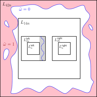
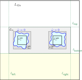
Figure 7: Two geometric argument in the proof of the renormalization inequality. Left: inside the domain bounded by an $\tilde{\omega}=0$ dual curve, by SMP and (30), there is a uniformly positive probability for an $\tilde{\omega}=0$ dual crossing in the long direction of each of the eight rectangles forming the sides of the annuli $L_{2n}^{\mathsf{left}}\setminus L_{n}^{\mathsf{left}}$ and $L_{2n}^{\mathsf{right}}\setminus L_{n}^{\mathsf{right}}$, as illustrated on the right side of $L_{2n}^{\mathsf{left}}\setminus L_{n}^{\mathsf{left}}$. For a simpler illustration, we have drawn the case when $L_{m}$ are squares, and the squares and the distances between them are not in scale. Right: by Proposition 8.2, there is a uniformly positive probability that the explored $\tilde{\omega}=0$ dual-loops (in blue) are separated by dual-curve(s) of $h\omega\leq 0$ from the area below the bottom line $\ell_{\mathsf{bottom}}$ of $\mathcal{L}_{3n}$ (in light yellow). Arguing similarly for the lines marking the top, left, and right sides of $\mathcal{L}_{3n}$, one obtains (34).

Next, let $(h,B,\omega)\sim\mathbb{P}_{L_{42n}}^{\pm 1}=:\mathbb{P}$ and set $\tilde{h}=6-h$ and define $\tilde{\omega}$ via $(\tilde{h},B)$. Then, with the above boundary condition, $\mathcal{O}^{*}_{\mathcal{E}}(L_{14n})=\mathcal{O}^{*}_{\tilde{\omega}=0}(L_{14n})$. On this event, by Lemma 4.5, exploring the boundary component of $\tilde{\omega}=1$ and its bounding $\tilde{\omega}=0$ dual curves generates a $\tilde{h}\in\{\pm 1\}$ boundary condition in the unexplored domains. Then, by (32) and the FKG for $\omega$, (see Figure 7 (left))

$$\mathbb{P}[\mathcal{O}_{\tilde{\omega}=0}^{*}(L_{n}^{\mathsf{left}},L_{2n}^{\mathsf{left}})\ \cap\mathcal{O}_{\tilde{\omega}=0}^{*}(L_{n}^{\mathsf{right}},L_{2n}^{\mathsf{right}})\;|\;\mathcal{O}^{*}_{\tilde{\omega}=0}(L_{14n})]\geq c_{1}^{8},$$

so

$$\mathbb{P}[\mathcal{O}_{\tilde{\omega}=0}^{*}(L_{n}^{\mathsf{left}},L_{2n}^{\mathsf{left}})\ \cap\mathcal{O}_{\tilde{\omega}=0}^{*}(L_{n}^{\mathsf{right}},L_{2n}^{\mathsf{right}})]\geq c_{1}^{8}b_{14n}.$$ (33)

Next, let us detect the occurrence of the intersection $\mathcal{I}:=\mathcal{O}_{\tilde{\omega}=0}^{*}(L_{n}^{\mathsf{left}},L_{2n}^{\mathsf{left}})\ \cap\mathcal{O}_{\tilde{\omega}=0}^{*}(L_{n}^{\mathsf{right}},L_{2n}^{\mathsf{right}})$ by exploring $\tilde{\omega}$ inside $L_{n}^{\mathsf{left}}$ and $L_{n}^{\mathsf{right}}$, and then outward up to the innermost dual-loops of $\tilde{\omega}=0$ surrounding them. For events that only depend on the exterior of these dual-loops, by the SMP, this exploration generates a boundary condition $\tilde{h}\in{\pm 1}$ (i.e., $h\in\{5,7\}$) on the dual-loops. Let $\mathcal{L}_{3n}$ be the “long lozenge”/long rectangle, obtained as the union of all horizontal translates of $L_{3n}$, when it is sled from $L^{\mathsf{left}}_{3n}$ to $L^{\mathsf{right}}_{3n}$, and let $\mathcal{S}_{h\omega\leq 0}^{*}$ be the event that $\mathcal{I}$ occurs and furthermore there is a dual path or dual-paths of $h\omega\leq 0$ that separate the above-mentioned two innermost loops from $\partial\mathcal{L}_{3n}$. Using Proposition 8.2 and the FKG for $(h,B)$ (in which crossings of $h\omega\leq 0$ are decreasing) and arguing as illustrated in Figure 7 (right),

$$\mathbb{P}[\mathcal{S}_{h\omega\leq 0}^{*}\;|\;\mathcal{I}]\geq c_{2}.$$ (34)

We next claim that

$$\mathbb{P}[\mathcal{O}_{h\omega\leq 0}^{*}(L^{\mathsf{left}}_{2n},L^{\mathsf{left}}_{3n})\cap\mathcal{O}_{h\omega\leq 0}^{*}(L^{\mathsf{right}}_{2n},L^{\mathsf{right}}_{3n})\;|\;\mathcal{I}\cap\mathcal{S}_{h\omega\leq 0}^{*}]\geq c_{3}.$$ (35)

Assuming this for a moment, the proof is readily finished; namely, observing that $\mathcal{I}\subset\mathcal{O}_{\mathcal{E}}^{*}(L_{n}^{\mathsf{left}},L_{2n}^{\mathsf{left}})\cap\mathcal{O}_{\mathcal{E}}^{*}(L_{n}^{\mathsf{right}},L_{2n}^{\mathsf{right}})$ we then have

$$\mathbb{P} [\mathcal{O}_{h\omega\leq 0}^{*}(L^{\mathsf{left}}_{2n},L^{\mathsf{left}}_{3n})\cap\mathcal{O}_{h\omega\leq 0}^{*}(L^{\mathsf{right}}_{2n},L^{\mathsf{right}}_{3n})\cap\mathcal{O}_{\mathcal{E}}^{*}(L_{n}^{\mathsf{left}},L_{2n}^{\mathsf{left}})\cap\mathcal{O}_{\mathcal{E}}^{*}(L_{n}^{\mathsf{right}},L_{2n}^{\mathsf{right}})] \geq c_{3}c_{2}c_{1}^{8}b_{14n}$$

and in particular

$$\mathbb{P}[\mathcal{O}_{\mathcal{E}}^{*}(L_{n}^{\mathsf{left}},L_{2n}^{\mathsf{left}})\cap\mathcal{O}_{\mathcal{E}}^{*}(L_{n}^{\mathsf{right}},L_{2n}^{\mathsf{right}})\;|\;\mathcal{O}_{h\omega\leq 0}^{*}(L^{\mathsf{left}}_{2n},L^{\mathsf{left}}_{3n})\cap\mathcal{O}_{h\omega\leq 0}^{*}(L^{\mathsf{right}}_{2n},L^{\mathsf{right}}_{3n})]\geq c_{3}c_{2}c_{1}^{8}b_{14n}.$$ (36)

Now, to detect the conditioning event above, explore $h$ and $\omega$ outside of $L^{\mathsf{left}}_{3n}$ and $L^{\mathsf{right}}_{3n}$, and inside them explore from the boundary until finding the exterior-most $h\omega\leq 0$ dual-loops surrounding $L^{\mathsf{left}}_{2n}$ and $L^{\mathsf{right}}_{2n}$, respectively. This generates a boundary condition $\preceq\{\pm 1\}$ for the unexplored (random) simply-connected domains $\mathcal{D}_{L}$ and $\mathcal{D}_{R}$ containing $L^{\mathsf{left}}_{2n}$ and $L^{\mathsf{right}}_{2n}$, respectively. By SMP, CBC and inclusion,

$$\mathbb{P} [\mathcal{O}_{\mathcal{E}}^{*}(L_{n}^{\mathsf{left}},L_{2n}^{\mathsf{left}})\cap\mathcal{O}_{\mathcal{E}}^{*}(L_{n}^{\mathsf{right}},L_{2n}^{\mathsf{right}})\;|\;\mathcal{D}_{L}=D_{L},\mathcal{D}_{R}=D_{R}]$$

$$\leq\mathbb{P}_{D_{L}}^{\pm 1}[\mathcal{O}_{\mathcal{E}}^{*}(L_{n}^{\mathsf{left}},L_{2n}^{\mathsf{left}})]\mathbb{P}_{D_{R}}^{\pm 1}[\mathcal{O}_{\mathcal{E}}^{*}(L_{n}^{\mathsf{right}},L_{2n}^{\mathsf{right}})]$$

$$\leq\mathbb{P}_{D_{L}}^{\pm 1}[\mathcal{O}_{\mathcal{E}^{\prime}}^{*}(L_{n}^{\mathsf{left}},L_{2n}^{\mathsf{left}})]\mathbb{P}_{D_{R}}^{\pm 1}[\mathcal{O}_{\mathcal{E}^{\prime}}^{*}(L_{n}^{\mathsf{right}},L_{2n}^{\mathsf{right}})],$$

where $\mathcal{E}^{\prime}$ is the set of edges on which $|h|\geq 5$ at both endpoints and additionally $B=0$ on edges between two absolute-heights $|h|=5$. By FKG for $(|h|,-B)$ and inclusion, and then sign flip symmetry

$$\mathbb{P}_{D_{L}}^{\pm 1}[\mathcal{O}_{\mathcal{E}^{\prime}}^{*}(L_{n}^{\mathsf{left}},L_{2n}^{\mathsf{left}})]\leq\mathbb{P}_{L_{3n}^{\mathsf{left}}}^{\pm 1}[\mathcal{O}_{\mathcal{E}^{\prime}}^{*}(L_{n}^{\mathsf{left}},L_{3n}^{\mathsf{left}})]\leq 2\mathbb{P}_{L_{3n}^{\mathsf{left}}}^{\pm 1}[\mathcal{O}_{\mathcal{E}}^{*}(L_{n}^{\mathsf{left}},L_{3n}^{\mathsf{left}})]=2b_{n}.$$

The same bound holds for $D_{R}$, and is independent of the shape of $D_{L}$ or $D_{R}$. Averaging over all $D_{L}$ and $D_{R}$, we thus have

$$\mathbb{P}[\mathcal{O}_{\mathcal{E}}^{*}(L_{n}^{\mathsf{left}},L_{2n}^{\mathsf{left}})\cap\mathcal{O}_{\mathcal{E}}^{*}(L_{n}^{\mathsf{right}},L_{2n}^{\mathsf{right}})\;|\;\mathcal{O}_{h\omega\leq 0}^{*}(L^{\mathsf{left}}_{2n},L^{\mathsf{left}}_{3n})\cap\mathcal{O}_{h\omega\leq 0}^{*}(L^{\mathsf{right}}_{2n},L^{\mathsf{right}}_{3n})]\leq 4b_{n}^{2},$$

which combined with (36) yields

$$b_{14n}\leq\tfrac{4}{c_{1}^{8}c_{2}c_{3}}b_{n}^{2}.$$

This concludes the proof.   $\square$

Proof of Equation (35)

In order to detect whether $\mathcal{I}\cap\mathcal{S}_{h\omega\leq 0}^{*}$ occurs, explore (i) the components of $\tilde{\omega}=1$ of $L^{\mathsf{left}}_{n}$ and $L^{\mathsf{right}}_{n}$, and their bounding dual-loops of $\tilde{\omega}=0$; and (ii) the component of $h\omega\geq 1$ of $\partial\mathcal{L}_{3n}$ in $\mathcal{L}_{3n}$ and its bounding dual-loops of $h\omega\leq 0$. The former finds the interior-most dual-loops of $\tilde{\omega}=0$ surrounding $L^{\mathsf{left}}_{n}$ and $L^{\mathsf{right}}_{n}$, and the latter the exterior-most loop(s) of $h\omega\leq 0$ separating them from $\partial\mathcal{L}_{3n}$.

Denote by $\mathcal{Y}$ the random unexplored area(s) between there explorations; it thus either consists of “two topological annuli” or a “simply-connected domain with two holes”. By SMP, on $\mathcal{Y}=Y$, the exploration generates a boundary condition $\chi$ taking values $\preceq\{\pm 1\}$ on the “outer boundary components” and the set-value $\{5,7\}$ on the “hole boundary components”. Let $R_{\mathsf{left}}$ be the “right rectangle of the annulus $L^{\mathsf{left}}_{3n}\setminus L^{\mathsf{left}}_{2n}$” and let $R_{\mathsf{right}}$ be the “left rectangle of the annulus $L^{\mathsf{right}}_{3n}\setminus L^{\mathsf{right}}_{2n}$”. We claim that

$$\mathbb{P}_{Y}^{\chi}[\mathcal{V}^{*}_{h\omega\leq 0}(R_{\mathsf{left}})\cup\mathcal{V}^{*}_{h\omega\leq 0}(R_{\mathsf{right}})]\geq c_{3}$$ (37)

for all $Y$, where for $(h,B,\omega)\sim\mathbb{P}_{Y}^{\chi}$ we interpret that $h\omega\leq 0$ on $Y^{c}$. Averaging over $Y$ then gives (35).

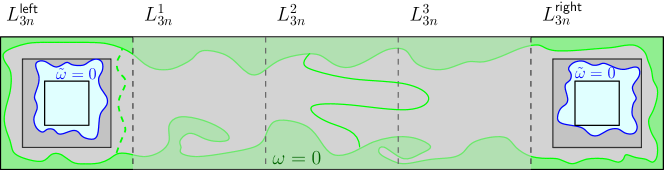
Figure 8: A geometric argument in the proof of Equation (35) (informal illustration): first, the random unexplored domain $\mathcal{Y}$ (in different shades of gray) can be compared to $\mathcal{L}=L_{3n}^{1}\cup L_{3n}^{2}\cup L_{3n}^{3}$, in which the probability of a vertical $h\omega\leq 0$ dual-corssing (in solid green) is lower-bounded by Corollary 7.5. Then, by Proposition 8.1, such a dual-crossing may be pushed into $L_{3n}^{\mathsf{left}}$ (dashed green).

It thus remains to prove (37). Denote $\mathcal{L}=L_{3n}^{1}\cup L_{3n}^{2}\cup L_{3n}^{3}$. We start by claiming that (see Figure 8)

$$\mathbb{P}_{Y}^{\chi}[\mathcal{V}^{*}_{h\omega\leq 0}(\mathcal{L})]\geq 1/8.$$ (38)

Indeed, letting $\chi^{\prime}$ be exactly $\{\pm 1\}$ on the outer boundary of $Y$, CBC gives

$$\mathbb{P}_{Y}^{\chi}[\mathcal{V}^{*}_{h\omega\leq 0}(\mathcal{L})]\geq\mathbb{P}_{Y}^{\chi^{\prime}}[\mathcal{V}^{*}_{h\omega\leq 0}(\mathcal{L})],$$

and with the boundary condition $\chi^{\prime}$, $\mathcal{V}^{*}_{h\omega\leq 0}(\mathcal{L})=\mathcal{V}^{*}_{\mathcal{E}^{\prime}(\tilde{h},B)}(\mathcal{L})$, and thus by the FKG for $(|\tilde{h}|,-B)$,

$$\mathbb{P}_{Y}^{\chi^{\prime}}[\mathcal{V}^{*}_{h\omega\leq 0}(\mathcal{L})]=\mathbb{P}_{Y}^{\chi^{\prime}}[\mathcal{V}^{*}_{\mathcal{E}^{\prime}(\tilde{h},B)}(\mathcal{L})]\geq\mathbb{P}_{\mathcal{L}\cap Y}^{\chi^{\prime\prime}}[\mathcal{V}^{*}_{\mathcal{E}^{\prime}(\tilde{h},B)}(\mathcal{L})]=\mathbb{P}_{\mathcal{L}\cap Y}^{\chi^{\prime\prime}}[\mathcal{V}^{*}_{h\omega\leq 0}(\mathcal{L})],$$

where $\chi^{\prime\prime}$ is the boundary condition for $\mathcal{H}_{\mathcal{L}\cap Y}$ on $\partial(\mathcal{L}\cap Y)$ which is, in terms of $h$, on the outer boundary of $Y$ equal to $\chi^{\prime}$, i.e., set-valued $h\in\{\pm 1\}$, and on the rest of $\partial(\mathcal{L}\cap Y)$ it is the largest admissible extension to $\{5,7\}$. Corollary 7.5 the gives (38).

The rest of proving (37) is easy; by exploring the left-most crossing generating $\mathcal{V}^{*}_{h\omega\leq 0}(\mathcal{L})$ and then applying Proposition 8.1, one obtains

$$\mathbb{P}_{Y}^{\chi}[\mathcal{V}^{*}_{h\omega\leq 0}(R_{\mathsf{left}})\;|\;\mathcal{V}^{*}_{h\omega\leq 0}(\mathcal{L})]\geq c_{4},$$

and thus

$$\mathbb{P}_{Y}^{\chi}[\mathcal{V}^{*}_{h\omega\leq 0}(R_{\mathsf{left}})]\geq c_{4}/8$$

and similarly for $\mathcal{V}^{*}_{h\omega\leq 0}(R_{\mathsf{right}})$. Finally, by the FKG for $(h,B)$

$$\mathbb{P}_{Y}^{\chi}[\mathcal{V}^{*}_{h\omega\leq 0}(R_{\mathsf{left}})\cup\mathcal{V}^{*}_{h\omega\leq 0}(R_{\mathsf{right}})]\geq\mathbb{P}_{Y}^{\chi}[\mathcal{V}^{*}_{h\omega\leq 0}(R_{\mathsf{left}})]\mathbb{P}_{Y}^{\chi}[\mathcal{V}^{*}_{h\omega\leq 0}(R_{\mathsf{right}})]\geq c_{4}^{2}/64.$$

This concludes the proof of (37), and hence also (35).   $\square$

10.2 Part (i) of Theorem 6.3

We start with an interesting extension of Theorem 6.2 which crucially uses the RSW theorem 9.1.

Lemma 10.1

Suppose that alternative (ii) of Theorem 6.2 occurs. Then, there exist $C,c,\alpha>0$ such that

$$\mathbb{P}_{L_{4n}}^{\pm 1}[\mathcal{O}^{*}_{\omega=0}(L_{n},L_{2n})]\geq 1-Ce^{-cn^{\alpha}}\qquad\text{for all }n.$$

Proof

Start by observing that $\mathcal{O}_{\omega=0}^{*}(L_{n},L_{2n})^{c}$ equivalently means that there is a primal-crossing of $\omega=1$ from $\partial L_{2n}$ to $\partial L_{n}$. Let $R$ denote a translate of $R_{5n/2,n/2}$ that covers the “bottom rectangle” of $L_{2n}\setminus L_{n}$. If such a primal-crossing lands on the bottom of $\partial L_{2n}$, it necessarily induces $\mathcal{V}_{\omega=1}(R)$. Combining these observation with the symmetric roles of the sides of $L_{2n}$, one obtains

$$1-\mathbb{P}_{L_{4n}}^{\pm 1}[\mathcal{O}^{*}_{\omega=0}(L_{n},L_{2n})]\leq 4\mathbb{P}_{L_{4n}}^{\pm 1}[\mathcal{V}_{\omega=1}(R)].$$

By Theorem 9.1 and simple FKG arguments, there exist $c^{\prime},C^{\prime}>0$ such that

$$c^{\prime}\mathbb{P}_{L_{4n}}^{\pm 1}[\mathcal{V}_{\omega=1}(R)]^{C^{\prime}}\leq b_{n}.$$

The claim now follows from alternative (ii) of Theorem 6.2 (as $b_{n}\leq a_{n}$ by (29)).   $\square$

Proof of of Part (i) in Theorem 6.3

Let $L^{j}$, $j=1,2,\ldots$, be $x$-centered lozenges or squares, with side length $k2^{j}$ horizontal periods. Fix $J$ and study $(h,B,\omega)\sim\mathbb{P}^{\pm 1}_{L^{J}}=:\mathbb{P}_{J}$; note that there exists $C>0$, depending only on $\mathbb{G}$ and its bi-periodic structure, such that if $|h(x)|\geq Ck$, then $\omega=1$ on the entire $L^{2}$. In particular, if $|h(x)|\geq Ck$, there exist a largest value of $j\in\{3,4,\ldots,J-1\}$ for which $\mathcal{O}^{*}_{\omega=0}(L^{j-2},L^{j-1})$ does not occur (and $\mathcal{O}^{*}_{\omega=0}(L^{j-1},L^{j})$ occurs, where we count $\partial L^{J}$ as a dual-loop of $\omega=0$ if $j=J$); let $\mathcal{E}_{\ell}$ be the event that this largest value of $j$ is $\ell$. We thus have

$$\mathbb{P}_{J}[|h(x)|\geq Ck] \leq\mathbb{P}_{J}[\bigcup_{\ell=3}^{J-1}\mathcal{E}_{\ell}]$$

$$\leq\sum_{\ell=3}^{J-1}\mathbb{P}_{J}[\mathcal{O}^{*}_{\omega=0}(L^{\ell-2},L^{\ell-1})^{c}\cap\mathcal{O}^{*}_{\omega=0}(L^{\ell-1},L^{\ell})].$$

An exploration argument to detect $\mathcal{O}^{*}_{\omega=0}(L^{\ell-1},L^{\ell})$ and FKG yield

$$\mathbb{P}_{J}[\mathcal{O}^{*}_{\omega=0}(L^{\ell-2},L^{\ell-1})^{c}\;|\;\mathcal{O}^{*}_{\omega=0}(L^{\ell-1},L^{\ell})]\leq\mathbb{P}^{\pm 1}_{L^{\ell}}[\mathcal{O}^{*}_{\omega=0}(L^{\ell-2},L^{\ell-1})^{c}]\leq C^{\prime}e^{-c(k2^{\ell})^{\alpha}},$$

where the latter inequality follows due to Lemma 10.1. Combining the two previous displayed equations,

$$\mathbb{P}_{J}[|h(x)|\geq Ck]\leq\sum_{\ell=3}^{\infty}C^{\prime}e^{-c(k2^{\ell})^{\alpha}}.$$

Note that the right-hand side is independent of $J$. It readily implies (e.g., by computing the obvious integral upper-bound of the series above) that $\mathbb{E}_{J}[h(x)^{2}]$ is uniformly bounded in $J$, i.e., (Var-loc) occurs. This concludes the proof.   $\square$

10.3 Part (ii) of Theorem 6.3: lower bound

Proof of the lower bound in part (ii) of Theorem 6.3

By (FKG-—h—), it suffices to consider the case $D=L_{n}$, $x=0$. Denote now

$$v_{n}:=\mathrm{Var}^{0}_{L_{n}}h(0)=\mathbb{E}^{\{\pm 1\}}_{L_{n}}[h(0)^{2}].$$

Note that by the FKG for $|h|$, $v_{n}$ is thus increasing in $n$. It thus suffices to prove the lower bound of (ii) for powers of $R$ (i.e., the parameter $R=3$ from Theorem 6.2), $n_{k}=R^{k}$, one has

$$v_{n_{k+1}}\geq v_{n_{k}}+c,$$

for an absolute constant $c>0$. Denote below $\mathbb{P}^{\pm 1}_{L_{n_{k}}}=:\mathbb{P}_{k}$ for short.

Let thus $(h,B,\omega)\sim\mathbb{P}_{k+1}$ and define a percolation process $\nu$ on the edges by

$$\nu_{\langle u,v\rangle}=\begin{cases}0,\qquad\{|h(u)|,|h(v)|\}=\{5,7\}\\ B_{\langle u,v\rangle},\qquad|h(u)|=|h(v)|\in\{5,7\}\\ 1,\qquad\text{otherwise}.\end{cases}$$

Trivially,

$$v_{n_{k+1}}=\mathbb{P}_{k+1}[\mathcal{O}^{*}_{\nu=0}(L_{n_{k}})]\mathbb{E}_{k+1}[h(0)^{2}\;|\;\mathcal{O}^{*}_{\nu=0}(L_{n_{k}})]+\mathbb{P}_{k+1}[\mathcal{O}^{*}_{\nu=0}(L_{n_{k}})^{c}]\mathbb{E}_{k+1}[h(0)^{2}\;|\;\mathcal{O}^{*}_{\nu=0}(L_{n_{k}})^{c}].$$

where, by the assumed (loop-deloc)

$$\mathbb{P}_{k+1}[\mathcal{O}^{*}_{\nu=0}(L_{n_{k}})]\geq\mathbb{P}_{k+1}[\mathcal{O}^{*}_{\mathcal{E}}(L_{n_{k}})]\geq\tfrac{1}{2C}.$$

Now, detect the event $\mathcal{O}^{*}_{\nu=0}(L_{n_{k}})$ by exploring the cluster of $\nu>0$ of the boundary $\partial L_{n_{k+1}}$ in $L_{n_{k+1}}\setminus L_{n_{k}}$, and its bounding $\nu=0$ dual-loops. If $\mathcal{O}^{*}_{\nu=0}(L_{n_{k}})$ does not occur, continue by revealing $\nu$ and $|h|$ on the entire $L_{n_{k+1}}\setminus L_{n_{k}}$ and $\partial L_{n_{k}}$. Note that now that when $|h|$ is known, $\nu$ equivalently provides information only about $B_{\langle u,v\rangle}$ on the edges where $|h(u)|=|h(v)|\in\{5,7\}$. In particular, since $B$ and $h$ are independent, this exploration provides an absolute-value boundary condition. Using then (SMP-—h—) and (CBC-—h—), one obtains

$$\mathbb{E}_{k+1}[h(0)^{2}\;|\;\mathcal{O}^{*}_{\nu=0}(L_{n_{k}})^{c}]\geq\mathbb{E}_{k}[h(0)^{2}]=v_{k}.$$

In the complementary case where $\mathcal{O}^{*}_{\nu=0}(L_{n_{k}})$ does occur, the exploration above generates by SMP a boundary condition $h\in\{5,7\}$ or $h\in\{-5,-7\}$ for the unexplored simply-connected domain $\mathcal{D}\supset L_{n_{k}}$. Then, compute

$$\mathbb{E}_{\mathcal{D}}^{\pm\{5,7\}}[h(0)^{2}]=\mathbb{E}_{\mathcal{D}}^{\pm 1}[(h(0)\pm 6)^{2}]=\mathbb{E}_{\mathcal{D}}^{\pm 1}[h(0)^{2}]+36\geq v_{k}+36,$$

where in the second step we used the sign flip symmetry to deduce $\mathbb{E}_{\mathcal{D}}^{\pm 1}[h(0)]=0$, and in the third the FKG for $|h|$. Combining the four previously displayed inequalities, we obtain

$$v_{n_{k+1}}\geq v_{k}+\tfrac{18}{C}.$$

This proves the claim.   $\square$

10.4 Part (ii) of Theorem 6.3: upper bound

Throughout this subsection, by mapping the bi-periodic embedding of $\mathbb{G}$ linearly if needed, we will assume that $\mathbb{G}$ is $\mathbb{Z}^{2}$ translation invariant. (Only the translational symmetries of $\mathbb{G}$ will be needed, and this will hence simplify the presentation.) Denote by $\mathbb{T}_{N}$ denote the “locally $\mathbb{G}$” graph on the torus, obtained by identifying the top and bottom (resp. left and right) sides of $\mathbb{G}\cap[-N,N]^{2}$. Denote by $\mathbb{E}_{\mathbb{T}_{N}}$ the random Lipschitz model on $\mathbb{T}_{N}$, with the boundary condition $h(r)\in\{\pm 1\}$ imposed only at an auxiliary root node $r$ (which often, such as in the theorem below, need not be specified). The main result of this subsection is the following.

Proposition 10.2

Suppose that (loop-deloc) occurs in Theorem 6.2. Then, there exists $C>0$ such that for all $N$ and all $x,y\in V(\mathbb{T}_{N})$ with $d_{\mathbb{T}_{N}}(x,y)\geq 2$, we have

$$\mathbb{E}_{\mathbb{T}_{N}}[(h(x)-h(y))^{2}]\leq\log Cd_{\mathbb{T}_{N}}(x,y),$$

where $d_{\mathbb{T}_{N}}$ denotes the graph distance.

Let us see how this concludes the proof of Theorem 6.3.

Proof of the upper bound in part (ii) of Theorem 6.3

Embed $D$ on a torus $\mathbb{T}_{N}$ (with $N$ large enough to fit $D$ on $\mathbb{T}_{N}$); let $y$ be the closest boundary point to $x$ on $\partial D$, and set $r=y$ for the torus measure. By FKG for $(|h|,\omega)$ and then SMP

$$\mathbb{E}_{\mathbb{T}_{N}}[h(x)^{2}]\geq\mathbb{E}_{\mathbb{T}_{N}}[h(x)^{2}\;|\;\omega_{D^{c}}=0]=\mathbb{E}_{D}^{\pm 1}[h(x)^{2}].$$ (39)

It is then readily observed that for $r=y$, we have

$$\mathbb{E}_{\mathbb{T}_{N}}[h(x)^{2}]=\mathbb{E}_{\mathbb{T}_{N}}[(h(x)-h(y))^{2}]+1,$$ (40)

which, by Proposition 10.2, concludes the proof.   $\square$

The rest of this subsection constitutes the proof of Proposition 10.2. For simplicity, shift $x$ to the origin, $x=0$, and define

$$w_{n}=\sup_{D:D^{c}\cap[-n,n]^{2}\neq\emptyset}\mathbb{E}^{\pm 1}_{D}[h(0)^{2}],$$

where the supremum is over finite subgraphs $D=(V,E)\ni x$ of $\mathbb{T}_{N}$ such that $y\in D^{c}\cup\partial D$ and that are (i) bounded inside a contractible loop on the toric dual $\mathbb{T}_{N}^{*}$ that surrounds $x$ but not $y$; or (ii) bounded outside a contractible loop on $\mathbb{T}_{N}^{*}$ that surrounds $y$ but not $x$; or (iii) bounded between two disjoint non-contractible loops on $\mathbb{T}_{N}^{*}$ that together separate $x$ from $y$. In all cases, the boundary condition $\{\pm 1\}$ is imposed on the primal-vertices adjacent to an edge crossing these bounding dual loops. Note that $w_{n}$ also depend on $y$ and $N$; we however keep this implicit in the notation; also, $w_{n}$ is manifestly increasing in $n$, and it suffices to study $w_{n}$ for $n\leq d_{\infty}(0,y)=\sup\{r:\bar{y}\not\in[-r,r]^{2}\}$, where $\bar{y}$ is the lift of $y\in\mathbb{T}_{N}$ to $[-N,N]^{2}$. Also, denote

$$u_{n}=w_{d_{\infty}(0,y)-n}.$$

The proof of Proposition 10.2 now boils down to the following lemma in two parts.

Lemma 10.3

Suppose that (loop-deloc) occurs in Theorem 6.2. Then, there exists $C>0$ independent of $N$, $y$ and $x$ such that

$$\text{i)}\qquad w_{2n}\leq w_{n}+C,\qquad\text{for all $n\leq d_{\infty}(0,y)/3$; and}$$ (41)

$$\text{ii)}\qquad u_{n}\leq u_{2n}+C,\qquad\text{for all $n\leq d_{\infty}(0,y)/3$.}$$ (42)

Remark 10.4

Readers only interested in simply-connected discrete domains may observe that any simply-connected domain can be embedded on a large enough torus. Then, (41) alone will be sufficient to conclude the upper bound of part (ii) of Theorem 6.3 for simply-connected domains. Consequently, such readers may restrict to “cases (i)” in several two-case formulations in the rest of this subsection.

Let us now see how Lemma 10.3 proves Proposition 10.2.

Proof of Proposition 10.2

Note first that $w_{1}$ is bounded by a constant that only depends on $\mathbb{G}$, due to the one-Lipschitzness of $h$. Equation (41) (and the fact that $w_{n}$ is increasing in $n$) then shows that

$$w_{n}\leq C^{\prime}\log n,\qquad\text{for all }n\leq 2d_{\infty}(0,y)/3$$

and similarly,

$$u_{1}\leq u_{n}+C^{\prime}\log n,\qquad\text{for all }n\leq 2d_{\infty}(0,y)/3;$$

here $C^{\prime}$ is independent of $N$, $x$ and $y$. Then note that by definition

$$w_{d_{\infty}(0,y)}-n=u_{n},$$

which we use for any fixed $d_{\infty}(0,y)/3\leq n\leq 2d_{\infty}(0,y)/3$. Also by definition and Lipschitzness, there exists $C^{\prime\prime}$ depending only on the bi-periodic lattice such that

$$\mathbb{E}_{\mathbb{T}_{N}}[(h(x)-h(y))^{2}]=\mathbb{E}^{\pm 1}_{\partial D=\{y\}}[h(0)^{2}]\leq u_{1}+C^{\prime\prime}.$$

The claim follows by combining the displayed inequalities.   $\square$

It thus remains to prove Lemma 10.3. We start with the following.

Lemma 10.5

Suppose that (loop-deloc) occurs in Theorem 6.2. Then, there exists $c>0$ such that the following holds for all $N,n,x,y$. Let $D_{m}\subset\mathbb{T}_{N}$ (resp. $D_{m}^{\prime}$) denote subgraphs as in the supremum defining $w_{m}$ (resp. $u_{m}$). Then,

$$\text{i)}\quad\mathbb{P}^{\pm 1}_{D_{2n}}[\partial D_{2n}\stackrel{{\scriptstyle h\leq_{B}5}}{{\longleftrightarrow}}[-n,n]^{2}]\geq c,\quad\text{for all $n\leq d(x,y)/3$; and}$$ (43)

$$\text{ii)}\quad\mathbb{P}^{\pm 1}_{D^{\prime}_{n}}[\partial D^{\prime}_{n}\stackrel{{\scriptstyle h\leq_{B}5}}{{\longleftrightarrow}}[-d_{\infty}(0,y)-2n,d_{\infty}(0,y)-2n]^{2}]\geq c,\quad\text{for all $n\leq d(x,y)/3$.}$$ (44)

Figure 9: The geometric setups in cases (i) (left) and (ii) (right) in the proof of Lemma 10.5.

Proof

The proof starts with a geometric setup that is different in the two cases (see Figure 9).

Case (i): Denote $D:=D_{2n}$, $S_{x}:=[-n,n]$ and $S_{x}^{\prime}:=[-2n,-2n]^{2}$. The claim is immediate if $\partial D$ intersects $S_{x}$, so assume not. Divide $S_{x}^{\prime}\setminus S_{x}$ into $12$ translates of the square $[0,n]^{2}$; let $S$ be one such translate which additionally intersects $\partial D$. Let $S^{\prime}$ be a translate of $[0,3n]^{2}$, cocentric with $S$. Note that (i) $x$ lies on the (planar-domain) boundary of $S^{\prime}$; and (ii) $y$ lies outside of $S^{\prime}$ (since $n\leq d_{\infty}(x,y)/3$); and (iii) there exists a primal-path $\gamma$ in $S\cap D$ from $\partial S_{x}$ to $\partial D$.

Case (ii): Denote $D:=D^{\prime}_{n}$, $S_{x}:=[-d_{\infty}(0,y)-2n,d_{\infty}(0,y)-2n]^{2}$ and $S_{x}^{\prime}:=[-d_{\infty}(0,y)-n,d_{\infty}(0,y)-n]^{2}$. The claim is immediate if $\partial D$ intersects $S_{x}$, so assume not. Let $S$ be a translate of $[0,n]^{2}$ that lies in $S_{x}^{\prime}\setminus S_{x}$ and intersects $\partial D$; let $S^{\prime}$ be a translate of $[0,3n]^{2}$, cocentric with $S$. Now, both $x$ and $y$ lie outside of $S^{\prime}$ and there exists a primal-path $\gamma$ in $S\cap D$ from $\partial S_{x}$ to $\partial D$

The rest of the proof is identical in the two cases. Denote by $E$ the event in Equation (43) or (44), and suppose that $E$ does not occur; hence, there exists a dual-curve of $\mathcal{E}$ that disconnects $y$ and $\partial D$ from $x$ and $S_{x}$ (or possibly two dual-curves, if $\partial D$ does not surround $x$). This dual-curve must on the one hand cross the primal-path $\gamma$ to separate $\partial S_{x}$ and $\partial D$, and hence visit $S$, and on the other hand, it must exit $S^{\prime}$ (since both $x$ and $y$ are outside of it). I.e.,

$$E^{c}\subset\mathcal{C}_{\mathcal{E}}^{*}(S,S^{\prime}),$$

where $\mathcal{C}_{\mathcal{E}}^{*}(S,S^{\prime})$ denotes the existence of a dual-crossing on $\mathcal{E}^{*}$ from $S$ to $S^{\prime}$ in $S^{\prime}$. By a shift of boundary conditions and then FKG for $(|h|,\omega)$, we hence have

$$1-\mathbb{P}^{\pm 1}_{D}[E]\leq\mathbb{P}^{\pm 1}_{D}[\mathcal{C}_{\mathcal{E}}^{*}(S,S^{\prime})]=\mathbb{P}^{\{5,7\}}_{D}[\mathcal{C}_{\omega=0}^{*}(S,S^{\prime})]\leq\mathbb{P}^{\chi}_{S^{\prime}\cap D}[\mathcal{C}_{\omega=0}^{*}(S,S^{\prime})],$$

where $\chi$ is the boundary condition for $\mathcal{H}_{S^{\prime}\cap D}$ given on $\partial(S^{\prime}\cap D)$ which is $\{\pm 1\}$ on $\partial S^{\prime}$ and its largest extension to $\{5,7\}$ on the rest.

Next, for $\mathcal{H}_{S^{\prime}\cap D}$, interpret $h\geq 1$, $B=1$ and $\omega=1$ on $S^{\prime}\cap D^{c}$; hence by duality and the present boundary condition, $\mathcal{C}_{\omega=0}^{*}(S,S^{\prime})^{c}=\mathcal{O}_{h\omega\geq 1}(S,S^{\prime})$. Using this complement event, a height shift, and then the boundary condition and bound on dual-degree

$$\mathbb{P}^{\chi}_{S^{\prime}\cap D}[\mathcal{C}_{\omega=0}^{*}(S,S^{\prime})]=1-\mathbb{P}^{6-\chi}_{S^{\prime}\cap D}[\mathcal{O}_{h\leq_{B}5}(S,S^{\prime})]=1-\mathbb{P}^{6-\chi}_{S^{\prime}\cap D}[\mathcal{O}_{|h|\leq_{B}5}(S,S^{\prime})].$$

Next, by FKG for $(|h|,-B)$ and then height shift

$$\mathbb{P}^{6-\chi}_{S^{\prime}\cap D}[\mathcal{O}_{|h|\leq_{B}5}(S,S^{\prime})]\geq\mathbb{P}^{\{5,7\}}_{S^{\prime}}[\mathcal{O}_{|h|\leq_{B}5}(S,S^{\prime})]=\mathbb{P}^{\pm 1}_{S^{\prime}}[\mathcal{O}_{h\omega\geq 1}(S,S^{\prime})]\geq c,$$

where the boundary conditions $\{5,7\}$ and $\{\pm 1\}$ are imposed on $\partial S^{\prime}$, and the last step used (loop-deloc). This concludes the proof.   $\square$

Corollary 10.6

Suppose that (loop-deloc) occurs in Theorem 6.2. Then, there exists $\ell\in\mathbb{N}$ and $c^{\prime}>0$ such that the following holds for all $N,n,x,y$. Let $D_{m}\subset\mathbb{T}_{N}$ (resp. $D_{m}^{\prime}$) denote subgraphs as in the supremum defining $w_{m}$ (resp. $u_{m}$). Then,

$$\text{i)}\quad\mathbb{P}^{\pm 1}_{D_{2n}}[\partial D_{2n}\stackrel{{\scriptstyle|h|\leq_{B}6\ell-1}}{{\longleftrightarrow}}[-n,n]^{2}]\geq c^{\prime},\quad\text{for all $n\leq d(x,y)/3$; and}$$ (45)

$$\text{ii)}\quad\mathbb{P}^{\pm 1}_{D^{\prime}_{n}}[\partial D^{\prime}_{n}\stackrel{{\scriptstyle|h|\leq_{B}6\ell-1}}{{\longleftrightarrow}}[-d_{\infty}(0,y)-2n,d_{\infty}(0,y)-2n]^{2}]\geq c^{\prime},\quad\text{for all $n\leq d(x,y)/3$.}$$ (46)

Proof

By SMP and the previous lemma, one readily deduces that

$$\mathbb{P}^{\pm 1}_{D_{2n}}[\{\partial D_{2n}\stackrel{{\scriptstyle h\leq_{B}6\ell-1}}{{\longleftrightarrow}}[-n,n]^{2}\}^{c}]\leq(1-c)^{\ell},$$

where $c$ is the constant in the previous lemma. By choosing $\ell$ large enough, there exists $c^{\prime}>0$ such that $(1-c)^{\ell}\leq\tfrac{1-c^{\prime}}{2}$. Then, by sign flip symmetry

$$\mathbb{P}^{\pm 1}_{D_{2n}}[\{\partial D_{2n}\stackrel{{\scriptstyle|h|\leq_{B}6\ell-1}}{{\longleftrightarrow}}[-n,n]^{2}\}^{c}]\leq 2\mathbb{P}^{\pm 1}_{D_{2n}}[\{\partial D_{2n}\stackrel{{\scriptstyle h\leq_{B}6\ell-1}}{{\longleftrightarrow}}[-n,n]^{2}\}^{c}]\leq 1-c^{\prime}.$$

Equation (46) is proven identically.   $\square$

Proof of Lemma 10.3

We will prove (41); (42) is identical. Let $\ell$ and $c^{\prime}$ be the constants of the above corollary. Let $(h,B,\omega)\sim\mathbb{P}^{\pm 1}_{D_{2n}}:=\mathbb{P}$ and define a percolation process $\nu$ on the edges by

$$\nu_{\langle u,v\rangle}=\begin{cases}0,\qquad\{|h(u)|,|h(v)|\}=\{6\ell\pm 1\}\\ \tilde{B}_{\langle u,v\rangle},\qquad|h(u)|=|h(v)|\in\{6\ell\pm 1\}\\ 1,\qquad\text{otherwise};\end{cases}$$

in other words, the event $\{\partial D_{2n}\stackrel{{\scriptstyle|h|\leq_{B}6\ell-1}}{{\longleftrightarrow}}[-n,n]^{2}\}^{c}$ means that there exist $\nu=0$ dual-paths that separate $\partial D_{2n}$ from $[-n,n]^{2}$; denote this event by $E_{n}$. Trivially,

$$\mathbb{E}[h(0)^{2}]=\mathbb{P}[E_{n}]\mathbb{E}[h(0)^{2}\;|\;E_{n}]+\mathbb{P}[E_{n}^{c}]\mathbb{E}[h(0)^{2}\;|\;E_{n}^{c}].$$

where, by the assumed (loop-deloc) and the previous corollary

$$\mathbb{P}[E_{n}]\leq 1-c^{\prime}.$$

Quite similarly to the proof of the lower bound in Theorem 6.1, one obtains

$$\mathbb{E}[h(0)^{2}\;|\;E_{n}]\leq w_{2n}+36\ell^{2}\qquad\text{and}\qquad\mathbb{E}[h(0)^{2}\;|\;E_{n}^{c}]\leq w_{n}+36\ell^{2}.$$

Recalling that $w_{2n}\geq w_{n}$, the three previously displayed equalities give an upper bound for $\mathbb{E}[h(0)^{2}]=\mathbb{E}^{\pm 1}_{D_{2n}}[h(0)^{2}]$ uniformly in $D_{2n}$, and hence

$$w_{2n}\leq(1-c^{\prime})(w_{2n}+36\ell^{2})+c^{\prime}(w_{n}+36\ell^{2})\Leftrightarrow w_{2n}\leq w_{n}+36\ell^{2}/c^{\prime}.$$

Recalling the $\ell$ and $c^{\prime}$ were independent of $x,y,n,N$, the proof is complete.   $\square$

11 On the infinite-volume limit

We now formalize and prove Corollary 1.2 from the Introduction. This section mimics an unpublished corollary of the logarithmic delocalization of the six-vertex model [DKMO20+], produced by the author and Piet Lammers in 2020.

11.1 Gradient Gibbs measures

Let $D=(V,E)$ be any locally finite connected graph. A vector field $g$ on $D$ assigns to every directed version $(u,v)$ of an edge $\langle u,v\rangle\in E$ a value $g_{(u,v)}=-g_{(v,u)}$. If additionally the values of $g$ sum to zero over any (oriented) loop on $D$, we say that $g$ is a gradient (vector) field; indeed, such a vector field $g$ is obtained as the discrete gradient $g_{(u,v)}=h(v)-h(u)$ of a function $h:V\to\mathbb{R}$ which is unique up to additive constant.

For the rest of this section, we study the space of $\mathcal{S}$ vector fields on a planar cubic lattice $\mathbb{G}$, with the detailed assumptions given in Section 6.1, that only take values in $\{0,\pm 2\}$ on the directed edges. We equip the space $\mathcal{S}$ with the metric of local convergence and note that it is (sequentially) compact. Gradient fields of height functions on finite $D\subset\mathbb{G}$ are naturally embedded in $\mathcal{S}$ by continuing with the zero field outside of $D$.

A (random Lipschitz) gradient Gibbs measure ${\sf P}$ is supported on the (infinite-volume) gradient fields of $\mathcal{S}$ and has the property that given the values of $g\sim{\sf P}$ on the edges of a simple closed primal-loop $\ell$ on $\mathbb{G}$, which defines up to additive constant an integer-valued function $\xi$ on the vertices of $\ell$, the conditional law of $g$ inside $\ell$ is the gradient of a random Lipschitz function $h\sim\mathbb{P}^{\xi}$ (where $\xi$ is ${\sf P}$-a.s. admissible by the gradient-field support of ${\sf P}$).

By the results of [She05] (also [Lam22, Lam23]), under the setup of Theorem 6.1, there exists a unique translationally invariant, slope-zero gradient Gibbs measure ${\sf P}$ on $\mathbb{G}$. Translational invariance refers here to the translations that generate the bi-periodicity of $\mathbb{G}$, and slope-zero means that ${\sf E}[h(x)-h(y)]=0$ for any $x,y\in\mathbb{V}$, where $h$ is a field whose gradient is $g\sim{\sf P}$. A direct consequence (which should not be regarded as a new result; [Lam22]) is:

Corollary 11.1

Let $\mathbb{G}$ and $\mathbf{c}_{e}$ be as in Theorem 6.1. Then, the gradients of the toric random Lipschitz functions $h\sim\mathbb{P}_{\mathbb{T}_{N}}$ converge weakly as $N\to\infty$ to the unique translationally invariant slope-zero gradient Gibbs measure ${\sf P}$ on $\mathbb{G}$.

Proof

Since $\mathcal{S}$ is compact, extract a subsequence $N_{j}$ so that the gradients converge weakly to some limit. Any such limit inherits directly from $\mathbb{P}_{\mathbb{T}_{N_{j}}}$ translational invariance, zero slope and the Gibbs property. The uniqueness result above thus identifies any subsequential limit, and hence also the weak limit along the entire sequence $N\to\infty$.   $\square$

In combination with the main results of this paper, one obtains the logarithmic variance structure of the limiting gradient field.

Corollary 11.2

Let $\mathbb{G}$, $\mathbf{c}_{e}$ and ${\sf P}$ be as in the previous corollary. There exist $c,C>0$ such that for any $x,y\in\mathbb{V}$,

$$c\log d_{\mathbb{G}}(x,y)\leq{\sf E}[(h(x)-h(y))^{2}]\leq C\log d_{\mathbb{G}}(x,y).$$

Proof

By Theorem 6.1, Equation (39) and Proposition 10.2, there exist $c,C>0$ such that for any $N$ and $x,y\in V(\mathbb{T}_{N})$, we have

$$c\log d_{\mathbb{T}_{N}}(x,y)\leq\mathbb{E}_{\mathbb{T}_{N}}[(h(x)-h(y))^{2}]\leq C\log d_{\mathbb{T}_{N}}(x,y).$$

The weak limit inherits these bounds (note that $(h(x)-h(y))^{2}$ is for fixed $x,y$ a bounded random variable by Lipschitzness).   $\square$

The rest of this section establishes ${\sf P}$ as the infinite volume limit of random Lipschitz functions on planar domains.

Proposition 11.3

Let $\mathbb{G}$, $\mathbf{c}_{e}$ and ${\sf P}$ be as in the previous corollaries, let $M\in\mathbb{N}$, and let $D_{n}\subset\mathbb{G}$ be finite connected subgraphs generated by their vertices and $\xi_{n}$ (not even necessarily interval-valued) admissible boundary conditions on $\partial D_{n}$ with $\xi_{n}(x)\subset\{-M,\ldots,M\}$ for all $x\in\partial D_{n}$. Then, the gradients of $h\sim\mathbb{P}^{\xi_{n}}_{D_{n}}$ converge weakly to ${\sf P}$ as $D_{n}\to\mathbb{G}$.

11.2 Proof of Proposition 11.3

The proof consist in three steps which may all be of independent interest. First, we show that (loop-deloc) actually implies that loops at any height can be guaranteed with any probability; the price to pay is increasing the aspect ratio of the annulus for the loops. Secondly, we show a mixing of boundary conditions lemma, and thirdly a translational invariance estimate.

Recall that $\mathcal{E}_{m}=\mathcal{E}_{m}(h,B)$ denotes the edges $e=\langle u,v\rangle$ for which $h(u),h(v)\geq m$ and if $h(u)=h(v)=m$ then additionally $B_{e}=0$, and similarly, $\mathcal{E}^{\prime}_{m}=\mathcal{E}^{\prime}_{m}(h,B)$ denotes the edges $e=\langle u,v\rangle$ for which $|h(u)|,|h(v)|\geq m$ and if $|h(u)|=|h(v)|=m$ then additionally $B_{e}=0$

Lemma 11.4 (Loops at any height with any probability)

For all $m\in\mathbb{N}$ and $\epsilon>0$ there exists $\rho>0$ such that

$$\mathbb{P}^{\pm 1}_{D}[\mathcal{O}^{*}_{\mathcal{E}_{m}}(L_{n})]\geq 1-\epsilon\qquad\text{whenever }L_{\rho n}\subset D.$$

Proof

By FKG for $(|h|,-B)$ and (loop-deloc), whenever $L_{3n}\subset D$, one has

$$\mathbb{P}^{\pm 1}_{D}[\mathcal{O}^{*}_{\mathcal{E}^{\prime}_{5}}(L_{n})^{c}]\leq\mathbb{P}^{\pm 1}_{L_{3n}}[\mathcal{O}^{*}_{\mathcal{E}^{\prime}_{5}}(L_{n})^{c}]\leq 1-c.$$

Now, suppose that $L_{3^{r}n}\subset D$. Explore the primal-cluster of $(\mathcal{E}^{\prime}_{5})^{c}$ from $\partial D$ inside $L_{3^{r-1}n}$; this exploration either reveals $\mathcal{O}^{*}_{\mathcal{E}^{\prime}_{5}}(L_{3^{r-1}n})$ or if not, reveal $|h|$ on entire $L_{3^{r-1}n}^{c}$ and generate an absolute-value boundary condition which for events of $(|h|,-B)_{|L_{3^{r-1}n}}$ dominates $\mathbb{P}^{\pm 1}_{L_{3^{r-1}n}}$. Reasoning as above, one obtains

$$\mathbb{P}^{\pm 1}_{D}[\mathcal{O}^{*}_{\mathcal{E}^{\prime}_{5}}(L_{3^{r-2}n})^{c}]\leq(1-c)^{2},$$

and similarly for any $k\leq r$

$$\mathbb{P}^{\pm 1}_{D}[\mathcal{O}^{*}_{\mathcal{E}^{\prime}_{5}}(L_{3^{r-k}n})^{c}]\leq(1-c)^{k}.$$

We now define iteratively the following (possibly empty) finite collection of dual-loops $\ell_{1},\ell_{2},\ldots\ell_{L}$, surrounding $L_{n}$. The first one, $\ell_{1}$ is the exterior-most loop generating $\mathcal{O}^{*}_{\mathcal{E}^{\prime}_{5}}(L_{n})$; by SMP, exploring outside $\ell_{1}$ generates a boundary condition $\{5,7\}$ or $\{-5,-7\}$ on the simply-connected domain inside, both conditions appearing with equal probability. Now, if $\ell_{j}$ generated a boundary condition $\{6k\pm 1\}$ for some $k\in\mathbb{Z}$, set $\tilde{h}=h-6k$ and explore inside $\ell_{j}$ until the exterior-most loop generating $\mathcal{O}^{*}_{\mathcal{E}^{\prime}_{5}(\tilde{h},B)}(L_{n})$, if such exists.

Using the observations of the first paragraph, it is readily shown that, if $L_{3^{r}n}\subset D$, the number $L$ of loops is (or can be coupled to be) larger than the number of successes in $r$ independent coin tosses with success probability $c$. Also, conditional on the number $L$, the heights on the loops perform an $L$-step simple random walk, stepping up or down by $6$ units with equal probability. By properties of independent coin tosses and simple random walks, by taking $r$ large enough, one can ensure that the heights on the loops $\ell_{1},\ldots\ell_{L}$ reach any $m$ with any probability $1-\epsilon$.   $\square$

For the mixing lemma, we need a slightly more general version of Proposition 4.7 which also allows boundary conditions in terms of $\omega$. Hence, for a finite connected $D=(V,E)$, and given boundary condition $\xi$, $E^{\prime}\subset E$ and a percolation $\beta:E^{\prime}\to\{0,1\}$, denote $\mathbb{P}_{D}^{\xi}[\;\cdot\;|\omega_{E^{\prime}}=\beta]=:\mathbb{P}_{D}^{\xi,\beta}[\;\cdot\;]$ (we always assume $\mathbb{P}_{D}^{\xi}[\omega_{E^{\prime}}=\beta]>0$ below).

Lemma 11.5

Let $D$ be a finite connected graph, $\xi\preceq_{abs}\xi^{\prime}$ two absolute-value boundary conditions on $\Delta$, $\beta\leq\beta^{\prime}$ two percolations on $E^{\prime}$, and $F,G:\mathcal{H}_{D}\times\{0,1\}^{E}\to\mathbb{R}$ increasing functions; then we have

$$\mathbb{E}^{\xi,\beta}_{D}\big{[}F(|h|,\omega)\big{]}\leq\mathbb{E}^{\xi^{\prime},\beta^{\prime}}_{D}\big{[}F(|h|,\omega)\big{]}.$$ (47)

Proof sketch

Perhaps the most direct proof is to verify the Holley criterion for the pairs $|h|,\omega$. The irreducibility and initial states are almost identical to the case of $|h|$ alone (Appendix  B). For the stochastic domination criterion, there are two parts: updating $|h|$ at a vertex and updating $\omega$ at an edge. The former is almost identical the case of $|h|$ alone (whose proof is based on comparing the weights $W(h)$, and changing them to $W(h,B)$, where $(h,B)$ gives the correct $(h,\omega)$, has essentially no effect since $h$ and $B$ are independent and $B$ is fixed in the comparisons). The updating of $\omega$ is directly handled by the positive association of the FK-Ising model (by Corollary 2.5). $\square$

Corollary 11.6 (Mixing)

For any even $m\in\mathbb{N}$ and any $\epsilon>0$ there exists $\rho$ such that the following holds. For any $D\supset L_{\rho n}$ and any (not even necessarily interval-valued) boundary condition $\xi$ on $\partial D$ with $\xi(x)\subset[1,m-1]$ for all $x\in\partial D$, there is a coupling $\mathbb{P}$ of $h\sim\mathbb{P}_{D}^{\xi}$ and $h^{\prime}\sim\mathbb{P}_{D}^{m\pm 1}$ such that

$$\mathbb{P}[h=h^{\prime}\text{ on }L_{n}]\geq 1-\epsilon.$$

Proof

Pick $\rho$ by the previous lemma so that

$$\mathbb{P}_{D}^{m\pm 1}[\mathcal{O}^{*}_{\omega=0}(L_{n})]\geq 1-\epsilon.$$ (48)

Suppose first that $\xi$ is single-valued. Next we would, informally speaking, like to use “SMP for two coupled height functions”; we have however formulated no such result, but the following is a direct consequence of the definition of $\mathbb{P}^{\xi,\beta}_{D}$ as conditional laws:

Lemma 11.7

Let $\xi,\xi^{\prime}$ be an absolute-value boundary conditions, $E_{i}\subset E$ and $\beta_{i},\beta_{i}^{\prime}:E_{i}\to\{0,1\}$ such that $\mathbb{P}^{\xi,\beta_{i}}_{D}$ and $\mathbb{P}^{\xi^{\prime},\beta_{i}^{\prime}}_{D}$ exist. Let $E_{i+1}=E_{i}\cup\{e_{i+1}\}$ where $e_{i+1}$ is given by a deterministic function of the setup $(E_{i},\xi,\beta_{i},\xi^{\prime},\beta_{i}^{\prime})$. Then, for $\beta_{i+1}^{+}$ (resp. $\beta_{i+1}^{-}$) the extension of $\beta_{i}$ to $e_{i+1}$ by $1$ (resp. by $0$) we have

$$\mathbb{P}^{\xi,\beta_{i}}_{D}[\omega(e_{i+1})=1]\mathbb{P}^{\xi,\beta_{i+1}^{+}}_{D}[\;\cdot\;]+\mathbb{P}^{\xi,\beta_{i}}_{D}[\omega(e_{i+1})=0]\mathbb{P}^{\xi,\beta_{i+1}^{-}}_{D}[\;\cdot\;]=\mathbb{P}^{\xi,\beta_{i}}_{D}[\;\cdot\;],$$

and similarly for the “primed case”.

We then construct the coupling $\mathbb{P}$ via the following exploration algorithm: start from the absolute-value boundary condition $\xi$ and $\xi^{\prime}=\{m\pm 1\}$ on $\partial D$ and $E_{0}=\emptyset$; at this point there are no $\beta_{0},\beta_{0}^{\prime}$. At any step, given $E_{i}$ and $\beta_{i}\leq\beta_{i}^{\prime}$ let $e_{i+1}$ be $\beta_{i}^{\prime}$-connected to $\partial D$ (choose one by an arbitrary deterministic function on $\beta_{i}^{\prime}$:s), sample $\omega(e_{i+1})$ from its law under $\mathbb{P}^{\xi,\beta_{i}}_{D}$ and $\omega^{\prime}(e_{i+1})$ from its law under $\mathbb{P}^{\xi^{\prime},\beta_{i}^{\prime}}_{D}$, the two coupled so that $\omega(e_{i+1})\leq\omega^{\prime}(e_{i+1})$ (this is possible by Lemma 11.5) and independently of the previous randomness in the algorithm. Then define $\beta_{i+1}$ and $\beta_{i+1}^{\prime}$ by extending by these values to $e_{i+1}$. By construction, $\beta_{i}\leq\beta_{i}^{\prime}$ at all steps, and by the above lemma, the law of $(h,B,\omega)$ (resp. $(h^{\prime},B^{\prime},\omega^{\prime})$) obtained from the random measure $\mathbb{P}^{\xi,\beta_{i}}_{D}[\;\cdot\;]$ (resp. $\mathbb{P}^{\xi^{\prime},\beta_{i}^{\prime}}_{D}[\;\cdot\;]$) is $\mathbb{P}^{\xi}_{D}$ (resp. $\mathbb{P}^{\xi^{\prime}}_{D}$).

The algorithm stops exploring at the time $T$ when it has exhausted the (random) $\beta^{\prime}_{T}$-cluster of $\partial D$. Note that also $\beta_{T}=0$ on the dual-curves bounding this cluster. Then, by Lemma 4.5 ,$(h,B,\omega)$ and $(h^{\prime},B^{\prime},\omega^{\prime})$ under $\mathbb{P}^{\xi,\beta_{T}}_{D}[\;\cdot\;]$ and $\mathbb{P}^{\xi^{\prime},\beta_{T}^{\prime}}_{D}[\;\cdot\;]$ have the same law inside these dual-curves. We sample them to be the same inside. By (48), this algorithmic procedure yields the desired coupling.

For set-valued $\xi$, the measure $\mathbb{P}_{D}^{\xi}$ is a convex combination of the compatible single-valued boundary conditions (with the appropriate convex coefficients). The claim follows then by coupling each single-valued condition to $\mathbb{P}_{D}^{m\pm 1}$ as above.   $\square$

Corollary 11.8 (Translational invariance)

For any $\epsilon>0$ there exists $\rho$ such that for any $D\supset L_{\rho n}$ and its translate $D^{\prime}$ by one bi-periodicity unit, there is a coupling $\mathbb{P}$ of $h\sim\mathbb{P}_{D}^{\pm 1}$ and $h^{\prime}\sim\mathbb{P}_{D^{\prime}}^{\pm 1}$ such that

$$\mathbb{P}[h=h^{\prime}\text{ on }L_{n}]\geq 1-\epsilon.$$

Proof

Observe first that there exists an even $k\in\mathbb{N}$, depending only on $\mathbb{G}$ and its biperiodic structure, such that the absolute-value of a $\mathbb{P}_{D}^{\pm 1}$ or $\mathbb{P}_{D^{\prime}}^{\pm 1}$ height function is at most $(k-1)$ on $\partial(D\cap D^{\prime})$. By the previous Corollary, we then choose $\rho$ so that for any single-valued boundary condition $\xi$ on $\partial(D\cap D^{\prime})$ with $|\xi|\leq k-1$ there is a coupling $\mathbb{P}^{(\xi)}$ of $h_{*}\sim\mathbb{P}_{D\cap D^{\prime}}^{2k\pm 1}$ and $h_{**}\sim\mathbb{P}_{D\cap D^{\prime}}^{\xi+k}$ such that

$$\mathbb{P}^{(\xi)}[h_{*}=h_{**}\text{ on }L_{n}]\geq 1-\epsilon/2;$$

this coupling induces a conditional law $\mathbb{P}^{(\xi)}[\;\cdot\;|h_{*}]$ of $h_{**}$ given $h_{*}$.

A coupling $\mathbb{P}$ required in the present statement can now be constructed as follows. First, let $h_{*}\sim\mathbb{P}_{D\cap D^{\prime}}^{2k\pm 1}$ be a variable in the coupling space. Then, for any $\xi$ as above, define $h_{**}^{\xi}$ on the coupling space by having the $\mathbb{P}$-conditional law $\mathbb{P}^{(\xi)}[\;\cdot\;|h_{*}]$ given $h_{*}$, and so that $h_{**}^{\xi}$ for different $\xi$ are $\mathbb{P}$-conditionally independent given $h_{*}$.

Let the coupling space $\mathbb{P}$ furthermore contain $\tilde{h}\sim\mathbb{P}_{D}^{\pm 1}$ and $\tilde{h}^{\prime}\sim\mathbb{P}_{D^{\prime}}^{\pm 1}$, independent of each other and the above random variables $h_{*},(h_{**}^{\xi})_{\xi}$. Finally, define $h$ (resp. $h^{\prime}$) to coincide with $\tilde{h}$ (resp. $\tilde{h}^{\prime}$) on $(D\cap D^{\prime})^{c}$ and $\partial(D\cap D^{\prime})$, and to coincide inside $D\cap D^{\prime}$ with that $(h_{**}^{\xi}-k)$ where $\xi=\tilde{h}_{|\partial(D\cap D^{\prime})}$ (resp. $\xi=\tilde{h}^{\prime}_{|\partial(D\cap D^{\prime})}$). By the SMP, the marginal laws are still $h\sim\mathbb{P}_{D}^{\pm 1}$ and $h^{\prime}\sim\mathbb{P}_{D^{\prime}}^{\pm 1}$, and by the Union bound,

$$\mathbb{P}[h=h_{*}=h^{\prime}\text{ on }L_{n}]\geq 1-\epsilon.$$

This concludes the proof.   $\square$

Proof of Proposition 11.3

By Corollary 11.6, it suffices to prove the claim when $\xi_{n}=\{\pm 1\}$. The proof then follows that of Corollary 11.1: extract a subsequence $n_{j}$ so that the gradients of $h\sim\mathbb{P}^{\pm 1}_{D_{n_{j}}}$ converge weakly to some limit. Any such limit inherits from $\mathbb{P}^{\pm 1}_{D_{n_{j}}}$ a zero slope and the Gibbs property and, by Corollary 11.8, such a limit is also translationally invariant. This identifies the subsequential limit as ${\sf P}$, which is hence also the weak limit along the entire sequence $\mathbb{P}^{\pm 1}_{D_{n}}$.   $\square$

Appendix A Phases for coupled models

The purpose of this appendix is to briefly review two couplings of random Lipschitz functions to the random homomorphism model and phase characterizations that follow from those for the Lipschitz functions. There exist also other couplings from the Lipschitz functions, e.g. the Yadin bijection [Pel17] or most famously to the $n=2$ loop $O(n)$ model on the honeycomb lattice (or other $3$-regular lattices), but we omit these discussions, the former being non-planar and the latter well-studied.

A.1 The couplings

The random homomorphism model

Let $G=(V,E)$ be a finite, connected, bipartite graph; we declare the vertices of $G$ as even or odd according to the bipartition. A (graph) homomorphism $g:V\to\mathbb{Z}$ is a function with $|g(u)-g(v)|=1$ for all adjacent vertices $u$ and $v$, and such that $g$ is odd on the odd vertices and even on the even vertices.

Given a non-empty $\Delta\subset V$, and $\xi:\Delta\to\mathbb{Z}$ such that $g_{|\Delta}=\xi$ for some homomorphism $g$, the random homomorphism model $\mathbb{Q}^{\xi}_{G}$ on $G$ with boundary condition $\xi$ is the uniform measure on homomorphisms $g:V\to\mathbb{Z}$ with $g_{|\Delta}=\xi$. Set-valued boundary conditions can be defined analogously.

$\mathbf{c}=2$ and homomorphisms on dotted graphs

The first coupling is for bipartite graphs obtained by “dotting”: let $G=(V,E)$ be a finite connected graph and let $\dot{G}=(\dot{V},\dot{E})$ be the bipartite dotted graph of $G$ obtained, pictorially, by adding a vertex in the middle of each edge of $G$; we declare the vertices of $\dot{G}$ that were already present in $G$ as odd, and the vertices of $\dot{G}$ in the middle of the edges of $G$ as even. Restriction to odd vertices now clearly provides a surjection from homomorphisms on $\dot{G}$ to height functions on $G$, and a boundary condition $\xi$ on $\Delta\subset V$ is admissible for height functions on $G$ if and only if it is admissible for homomorphisms on $\dot{G}$. Furthermore, this surjection yields the following coupling, whose proof we leave for the reader.

Proposition A.1

Let $G=(V,E)$ be a finite connected graph, $\dot{G}=(\dot{V},\dot{E})$ its dotted bipartite graph, $\Delta\subset V$ and $\xi:\Delta\to\mathbb{Z}_{\mathrm{odd}}$ a (possibly set-valued) boundary condition admissible for random Lipschitz functions on $G$ (equivalently, for homomorphisms on $\dot{G}$). If $g\sim\mathbb{Q}^{\xi}_{\dot{G}}$, then its restriction $g_{|G}$ has the law $\mathbb{P}^{\xi}_{G}$ of random Lipschitz functions on $G$ with edge weights $\mathbf{c}_{e}=2$ for all $e\in E$.

$\mathbf{c}=\sqrt{2}$ and homomorphisms on triangle–star transformed graphs

We say that a finite connected graph $G=(V,E)$ is a triangulation if there is a collection of mutually edge-disjoint triangles $t_{1},\ldots,t_{m}$ that covers $E$. By a triangle, we mean here a cyclic path three distinct oriented edges $e_{1},e_{2},e_{3}$ (the endpoints of these edges need not be three distinct vertices). The triangle–star (or $\nabla$–$Y$) transform $G_{Y}=(V_{Y},E_{Y})$ of $G$ is the bipartite connected graph obtained by adding $m$ new vertices $\varpi_{1},\ldots,\varpi_{m}$ and replacing the edges of each triangle $t_{i}=(e^{i}_{1}=(u,v),e^{i}_{2}=(v,w),e^{i}_{3}=(w,u))$ by the three edges $\langle u,\varpi_{i}\rangle$, $\langle v,\varpi_{i}\rangle$, $\langle w,\varpi_{i}\rangle$. The vertices of $G_{Y}$ that were already present in $G$ are again declared as odd, and $\varpi_{1},\ldots,\varpi_{m}$ as even. Restriction again provides a surjection from homomorphisms on $G_{Y}$ to height functions on $G$, and a boundary condition $\xi$ on $\Delta\subset V$ is admissible for height functions if and only if it is admissible for homomorphisms.

Proposition A.2

Let $G=(V,E)$ be a finite connected triangulation graph, $G_{Y}=(V_{Y},E_{Y})$ its $\nabla$–$Y$ transform, let $\Delta\subset V$ and $\xi:\Delta\to\mathbb{Z}_{\mathrm{odd}}$ a (possibly set-valued) boundary condition admissible for random Lipschitz functions on $G$ (equivalently, for homomorphisms on $\dot{G}$). If $g\sim\mathbb{Q}^{\xi}_{G_{Y}}$, then its restriction $g_{|G}$ has the law $\mathbb{P}^{\xi}_{G}$ of random Lipschitz functions on $G$ with edge weights $\mathbf{c}_{e}=\sqrt{2}$ for all $e\in E$.

Proof

We say that a given height function $h\in\mathcal{H}_{G}$ is flat on a triangle $t_{i}=\{(u,v),(v,w),(w,u)\}$ if $h(u)=h(v)=h(w)$ (in the complementary case, one of the vertices has a different height that the two others). Now, we have

$$\#\{\text{ homomorphisms $g$ on $G_{Y}$ with }g_{|G}=h\}=2^{\#\{t_{i}:\;h\text{ flat on }t_{i}\}}.$$

Sampling a random height function on $G$ as $g_{|G}$, where $g\sim\mathbb{Q}^{\xi}_{G_{Y}}$, the probability of each height configuration $h$ with $h(x)\in\xi(x)$ for all $x\in\Delta$ is thus proportional to $2^{\#\{t_{i}:\;h\text{ flat on }t_{i}\}}$. On the other hand, sampling a random height function on $G$ from the law $\mathbb{P}^{\xi}_{G}$ (with $\mathbf{c}_{e}\equiv\sqrt{2}$) the probability of a configuration $h$ with $h(x)\in\xi(x)$ for all $x\in\Delta$ is proportional to

$$W(h) =\prod_{\begin{subarray}{c}t_{i}=\{(u,v),(v,w),(w,u)\}\\ 1\leq i\leq m\end{subarray}}\sqrt{2}^{\mathbb{I}\{h(u)=h(v)\}+\mathbb{I}\{h(v)=h(w)\}+\mathbb{I}\{h(w)=h(u)\}}$$

$$=\sqrt{2}^{m}\cdot 2^{\#\{t_{i}:\;h\text{ flat on }t_{i}\}}.$$

It follows that the two random height functions are equal in distribution.   $\square$

A.2 Phase characterizations

We now state some phase characterizations following from the main results of this paper by the above couplings. For the sake of brevity, we will not explicate how a “discrete domain” should be defined for each different lattice (to be coherent with the above couplings), thus leaving the statements just slightly informal. We also note that the Gibbs measure and variance dichotomies and their equivalence, similar to Section 5, hold for the random homomorphism model [CPST21]; we thus trust that the reader understands the terms localized or logarithmically delocalized.

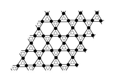
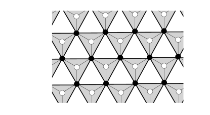
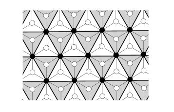
Figure 10: Top-left: The kagome lattice (black vertices, thick edges) is a triangulation and its $\nabla$–$Y$ transform is the dotted hexagonal lattice (both black and white vertices, thin edges). Top-right: an illustration of the same general idea of $Y$–$\nabla$ transforming of the dotted version of a $3$-regular lattice, in this case the square-octagon lattice. Bottom-left: The triangular lattice (black vertices, thick edges) is a triangulation (triangles filled with gray) and its $\nabla$–$Y$ transform is the hexagonal lattice (both black and white vertices, thin edges). Bottom-left: The triangular lattice with doubled edges (black vertices, thick edges, each edge doubled) is a triangulation (both white and gray triangles) and its $\nabla$–$Y$ transform is the rhombille lattice (both black and white vertices, thin edges).

1) The random homomorphism model on the dotted triangular lattice is localized. This holds due to its coupling to the $\mathbf{c}\equiv 2$ random Lipschitz model on the triangular lattice (Proposition A.1), which is localized by Corollary 3.2.

2) The random homomorphism model on the dotted honeycomb (resp. square-octagon) lattice (see Figure 10 (top-left)) is logarithmically delocalized, by its coupling to the $\mathbf{c}\equiv 2$ random Lipschitz model on the hexagonal lattice (Proposition A.1) and Theorem 6.1.

3) The random Lipschitz model with $\mathbf{c}\equiv\sqrt{2}$ on the kagome lattice (see Figure 10 (top-left)) is logarithmically delocalized, by its coupling to the random homomorphism model on the dotted hexagonal lattice (Proposition A.2).

3’) A non-quantitative delocalization can be similarly deduced for more general lattices. Let $\Gamma$ be any bi-periodic $3$-regular planar lattice. By [Lam22, Theorem 2.7] and [CPST21], the random homomorphism model is delocalized (but not necessarily logarithmically) on its bipartite dotted lattice $\dot{\Gamma}$. The odd vertices of this dotted lattice are all of degree $3$, and hence it is the star-triangle transform is a certain triangulation lattice, on which the $\mathbf{c}\equiv\sqrt{2}$ random Lipschitz model is delocalized. An example of this procedure with $\Gamma$ being the square-octagon lattice is illustrated in Figure 10(top-right). Theorem 6.1 shows that this delocalization is logarithmic for suitable lattices $\Gamma$, such as the illustrated case of the square-octagon lattice.

4) The random homomorphism model on the honeycomb lattice is logarithmically delocalized, by its coupling to the $\mathbf{c}\equiv\sqrt{2}$ random Lipschitz model on the triangular lattice (Proposition A.2; Figure 10 (bottom-left)) and the logarithmic delocalization of the latter [DGPS20]. It should be emphasized that (although a the heavy lifting for this result is [DGPS20]), the author is not aware of a prior explicit statement in the literature. The non-quantitative delocalization of this model follows by [Lam22, Theorem 2.7] and [CPST21].

5) The random homomorphism model on the rhombille lattice (Figure 10 (bottom-right)) is localized, by its coupling to the $\mathbf{c}\equiv\sqrt{2}$ random Lipschitz model on the triangular lattice with doubled edges (Proposition A.2). The latter is equivalent to $\mathbf{c}\equiv 2$ and non-doubled edges, which is localized by Corollary 3.2. This is arguably the simplest bipartite planar lattice on which the random homomorphism model is localized, highlighting the non-triviality of delocalization results such as the main result of the present paper.

Appendix B Positive association of the absolute-height

B.1 The Holley and FKG criteria

Let $D=(V,E)$ be a finite connected graph, and let $\mu$ and $\mu^{\prime}$ be two probability measures on $\mathcal{H}_{D}$. We say that $\mu^{\prime}$ stochastically dominates $\mu$, denoted $\mu\leq_{st}\mu^{\prime}$, if there exists a probability measure $\nu$ on pairs $(h,h^{\prime})\in\mathcal{H}_{D}\times\mathcal{H}_{D}$ such that the first and second marginal distributions are $\mu$ and $\mu^{\prime}$, respectively, and $\nu[h\preceq h^{\prime}]=1$. Note that if $\mu\leq_{st}\mu^{\prime}$, then, for all increasing $F:\mathcal{H}_{D}\to\mathbb{R}$,

$$\mu[F(h)]\leq\mu^{\prime}[F(h)].$$

We say that $\mu$ is irreducible if for any two $h,h^{\prime}\in\mathcal{H}_{D}$ with $\mu[h],\mu[h^{\prime}]>0$, there exists a finite sequence $h=h_{0},h_{1},\ldots,h_{m}=h^{\prime}$ on $\mathcal{H}_{D}$, such that for every $1\leq i\leq m$, $\mu[h_{i}]>0$ and $h_{i}$ differs from $h_{i-1}$ at one vertex only. We now recall the classical Holley and FKG criteria. For details see the extensive discussion of these criteria in [Gri06].

Lemma B.1 (Holley’s criterion)

Let $D=(V,E)$ be a finite connected graph, and $\mu,\mu^{\prime}$ probability measures on $\mathcal{H}_{D}$. The following criteria are sufficient to guarantee that $\mu\leq_{st}\mu^{\prime}$:

• $\mu$ and $\mu^{\prime}$ are irreducible; and

• there exist $h\preceq h^{\prime}\in\mathcal{H}_{D}$ such that $\mu[h]>0$ and $\mu^{\prime}[h^{\prime}]>0$; and

• for every vertex $x\in V$, every $k\in\mathbb{Z}_{\mathrm{odd}}$, $\mu$-almost every $\chi\in\mathcal{H}_{D\setminus\{x\}}$, and $\mu^{\prime}$-almost every $\chi^{\prime}\in\mathcal{H}_{D\setminus\{x\}}$ with $\chi\preceq\chi^{\prime}$, we have

  $$\mu[h(x)\geq k\;|\;h_{|G\setminus\{x\}}=\chi]\leq\mu^{\prime}[h(x)\geq k\;|\;h_{|G\setminus\{x\}}=\chi^{\prime}].$$ (49)

Lemma B.2 (FKG criterion)

Let $D=(V,E)$ be a finite connected graph, and $\mu$ an irreducible probability measure on $\mathcal{H}_{D}$. If for every vertex $x\in V$, every $k\in\mathbb{Z}_{\mathrm{odd}}$, and $\mu$-almost every $\chi\in\mathcal{H}_{G\setminus\{x\}}$ and $\chi^{\prime}\in\mathcal{H}_{G\setminus\{x\}}$ with $\chi\preceq\chi^{\prime}$, we have

$$\mu[h(x)\geq k\;|\;h_{|G\setminus\{x\}}=\chi]\leq\mu[h(x)\geq k\;|\;h_{|G\setminus\{x\}}=\chi^{\prime}],$$ (50)

then for all increasing functions $F_{1},F_{2}:\mathcal{H}_{G}\to\mathbb{R}$,

$$\mu[F_{1}(h)F_{2}(h)]\geq\mu[F_{1}(h)]\mu[F_{2}(h)].$$

B.2 Proof of Propositions 4.3 and 4.4

The inequality (CBC-—h—) follows by checking Holley’s criterion for $\mu$ the law of $|h|$ when $h\sim\mathbb{P}^{\xi}$ and $\mu^{\prime}$ the law of $|h^{\prime}|$ under $h^{\prime}\sim\mathbb{P}^{\xi^{\prime}}$. Then, by taking $\mu^{\prime}=\mu$ in the Holley criterion, we observe that $\mu$ satisfies the FKG criterion, which yields (FKG-—h—), so it is “a special case of” (CBC-—h—). Finally, (SMP-—h—) is proven via the Holley’s criterion for $\mu^{\prime}$ the law of $|h^{\prime}|$ when $h^{\prime}\sim\mathbb{P}^{\xi^{\prime}}_{D^{\prime}}$ and $\mu$ the law of $|h|$ when $h\sim\mathbb{P}^{\xi}_{D}$. The two verifications of Holley’s criterion are largely identical. Their proof consists of several routine computations and a nontrivial case of (49), where, roughly speaking, the sign of $h$ is not fixed around $x$ by $\chi$.

B.2.1 Routine computations

Irreducibility: We check the irreducibility of the law of $|h|$ with any absolute-value boundary condition $h\sim\mathbb{P}^{\xi}$. Let $H,H^{\prime}$ be absolute values of height functions $h,h^{\prime}\in\mathcal{H}_{D}$ allowed by $\xi$. It suffices to find a finite sequence of functions from $H$ to $H\vee H^{\prime}$; a similar path can be reversed from $H\vee H^{\prime}$ to $H^{\prime}$. For a lighter notation we assume $H\preceq H^{\prime}$. We’ll find a path $H=H_{0}\preceq H_{1}\preceq\ldots$ so that $H_{i}\preceq H^{\prime}$ and so that at each step, unless $H_{i}=H^{\prime}$, $H_{i}$ will be increased by $2$ at one vertex $x_{i}$ to obtain $H_{i+1}$. In finitely many steps, such a path will achieve $H^{\prime}$.

Now, if $H_{i}=H^{\prime}$ we’re done. Otherwise, we want to choose $x_{i}$. Note that $H_{i}(x_{i})$ can be lifted to yield another height function if and only if $x_{i}$ has no neighbours with a strictly lower height in $H_{i}$. Let $x_{i}\in V$ be the vertex where $H^{\prime}-H_{i}$ attains its maximum value; if there are several such vertices, pick one amongst them with minimal height $H_{i}(x_{i})$. It follows that $x_{i}$ cannot have neighbours with strictly lower height $H_{i}$, so its value can be increased, and $H_{i+1}$ thus obtained satisfies $H_{i+1}\preceq H^{\prime}$.

Initial states: We only need to consider the case of (CBC-—h—) here. Note that a function $\zeta:\Delta\to\mathbb{Z}_{\mathrm{odd}}$ is such that $\mathbb{P}^{\xi}[|h_{|\Delta}|=\zeta]>0$ if and only if it is an admissible single-valued boundary condition on $\Delta$ with $|a(x)|\leq\zeta(x)\leq b(x)$ for all $x\in\Delta$; we then say that $\zeta$ is $\mu$ possible. Let $\zeta$ and $\zeta^{\prime}$ be any $\mu$ and $\mu^{\prime}$ possible conditions, respectively. Since $\xi\preceq_{abs}\xi^{\prime}$, it follows that also $\zeta\wedge\zeta^{\prime}$ (resp. $\zeta\vee\zeta^{\prime}$) is $\mu$ possible (resp. $\mu^{\prime}$ possible). Let then $\overline{h}$ (resp. $\overline{h}^{\prime}$) be the maximal height function (3) with the boundary condition $\zeta\wedge\zeta^{\prime}$ (resp. $\zeta\vee\zeta^{\prime}$); hence $0<\overline{h}\preceq\overline{h}^{\prime}$. We also directly have $\mu[\overline{h}]=\mathbb{P}^{\xi}[|h|=\overline{h}]\geq\mathbb{P}^{\xi}[h=\overline{h}]>0$, and similarly for $\mu^{\prime}[\overline{h}^{\prime}]$.

Property (49): We start with trivialities. First, for (CBC-—h—) (resp. (SMP-—h—)), there is nothing to check if $x\in S^{\prime}\setminus S$ (resp. $x\in D^{\prime}\setminus D$). Second, we are actually proving a stochastic domination of real random variables. If $x\in\Delta$, the boundary conditions may restrict $H(x)$ (resp. $H^{\prime}(x)$) below (resp. above) some value (we denote $|h|=H$ and $|h^{\prime}|=H^{\prime}$ throughout the proof); stochastic domination for such conditional laws follows from that of the unconditional ones; thus little attention will be paid to the boundary conditions.

Let us denote by $M$ the maximum of $\chi^{\prime}$ on the neighbours $N_{x}$ of $x$, and by $m$ the minimum of $\chi$; thus $H(x)\leq m+2$ and $H^{\prime}(x)\geq M-2$ . If $M-m\geq 4$, we thus automatically have $H^{\prime}(x)\geq H(x)$. We hence assume $M-m\leq 2$ below; note that then the values of both $\chi$ and $\chi^{\prime}$ vary by at most $2$ on $N_{x}$.

Case 1: Suppose first that $m\geq 3$. This means that the sign of $h$ (and $h^{\prime}$ similarly) is constant on $N_{x}\cup\{x\}$ and, in particular, already the absolute value $H$ reveals, for any $y\in N_{x}$, whether $h(x)=h(y)$ or not (and for $H^{\prime}$ and $h^{\prime}$ similarly).

Case 1a: Suppose first that $\chi^{\prime}-\chi$ is a constant $0$ or $2$ on $N_{x}$. Then $h(x)$ behaves identically to $h^{\prime}(x)$ or $h^{\prime}(x)-2$, respectively, and (49) follows.

Case 1b: Suppose then that $\chi-\chi^{\prime}$ is not constant on $N_{x}$, and that both $\chi$ and $\chi^{\prime}$ take both values $m$ and $M=m+2$ on $N_{x}$. Then it necessarily occurs that $H(x),H^{\prime}(x)\in\{m,M\}$, and it suffices to show that

$$\frac{\mu[H(x)=M\;|\;H_{|D\setminus\{x\}}=\chi]}{\mu[H(x)=m\;|\;H_{|D\setminus\{x\}}=\chi]}\leq\frac{\mu^{\prime}[H^{\prime}(x)=M\;|\;H^{\prime}_{|D\setminus\{x\}}=\chi^{\prime}]}{\mu^{\prime}[H^{\prime}(x)=m\;|\;H^{\prime}_{|D\setminus\{x\}}=\chi^{\prime}]}.$$

We compute

$$\frac{\mu[H(x)=M\;|\;H_{|D\setminus\{x\}}=\chi]}{\mu[H(x)=m\;|\;H_{|D\setminus\{x\}}=\chi]}=\frac{\prod_{y\in N_{x}:\chi(y)=M}\mathbf{c}_{\langle x,y\rangle}}{\prod_{y\in N_{x}:\chi(y)=m}\mathbf{c}_{\langle x,y\rangle}},$$

and using a similar formula for the “primed case”,

$$\frac{\mu^{\prime}[H^{\prime}(x)=M\;|\;H^{\prime}_{|D\setminus\{x\}}=\chi^{\prime}]}{\mu^{\prime}[H^{\prime}(x)=m\;|\;H^{\prime}_{|D\setminus\{x\}}=\chi^{\prime}]}\Bigg{/}\frac{\mu[H(x)=M\;|\;H_{|D\setminus\{x\}}=\chi]}{\mu[H(x)=m\;|\;H_{|D\setminus\{x\}}=\chi]}=\prod_{y\in N_{x}:\chi^{\prime}(y)=M\;\&\;\chi(y)=m}\mathbf{c}_{\langle x,y\rangle}^{2}\geq 1.$$

Thus, (49) follows.

Case 1c: The remaining subcase is when $\chi-\chi^{\prime}$ is not constant on $N_{x}$, and exactly one out of $\chi$ and $\chi^{\prime}$ is a constant function on $N_{x}$. For definiteness, let us study the case $\chi^{\prime}_{|N_{x}}=M$, $\chi_{|N_{x}}\in\{M,M-2\}$ here (the other one is similar). $H^{\prime}(x)$ may thus take any of the values $\{M-2,M,M+2\}$, while $H(x)$ is either $M-2$ or $M$. It suffices to show that

$$\mu[H(x)=M\;|\;H_{|D\setminus\{x\}}=\chi]\leq\mu^{\prime}[H^{\prime}(x)\geq M\;|\;h_{|D\setminus\{x\}}=\chi^{\prime}].$$

The LHS becomes

$$\mu[H(x)=M\;|\;H_{|D\setminus\{x\}}=\chi] =\frac{\prod_{y\in N_{x}:\chi(y)=M}\mathbf{c}_{\langle x,y\rangle}}{\prod_{y\in N_{x}:\chi(y)=M}\mathbf{c}_{\langle x,y\rangle}+\prod_{y\in N_{x}:\chi(y)=m}\mathbf{c}_{\langle x,y\rangle}}$$

$$=\frac{\prod_{y\in N_{x}:\chi(y)=M}\mathbf{c}_{\langle x,y\rangle}/\prod_{y\in N_{x}:\chi(y)=m}\mathbf{c}_{\langle x,y\rangle}}{1+\prod_{y\in N_{x}:\chi(y)=M}\mathbf{c}_{\langle x,y\rangle}/\prod_{y\in N_{x}:\chi(y)=m}\mathbf{c}_{\langle x,y\rangle}}$$

while the RHS becomes

$$\mu^{\prime}[H^{\prime}(x)\geq M\;|\;h_{|D\setminus\{x\}}=\chi^{\prime}]=\frac{1+\prod_{y\in N_{x}}\mathbf{c}_{\langle x,y\rangle}}{1+1+\prod_{y\in N_{x}}\mathbf{c}_{\langle x,y\rangle}}.$$

Both are of the form $u/(1+u)$ which is increasing in $u\in\mathbb{R}_{+}$. We then deduce that the RHS is larger as $\mathbf{c}_{e}\geq 1$.

Case 2: Suppose now that $m=1$; thus, $H(x)$ is either $1$ or $3$.

Case 2a: Suppose also that $\chi^{\prime}_{|N_{x}}$ is a constant $3$. Thus, $H^{\prime}(x)$ may thus take any of the values $\{1,3,5\}$. It suffices to show that

$$\mu[H(x)=3\;|\;H_{|D\setminus\{x\}}=\chi]\leq\mu^{\prime}[H^{\prime}(x)\geq 3\;|\;h_{|D\setminus\{x\}}=\chi^{\prime}].$$

To compute the left-hand side we observe that, $H(x)=3$ can only occur if $\mathrm{sign}(h)$ is constant on $N_{x}$. Thus,

$$\mu[H(x)=3\;|\;H_{|D\setminus\{x\}}=\chi] =\mathbb{P}^{\xi}\big{[}\mathrm{sign}(h)\text{ cst. on }N_{x}\;|\;|h_{|D\setminus\{x\}}|=\chi\big{]}$$

$$\qquad\times\mathbb{P}^{\xi}\big{[}|h(x)|=3\;|\;\mathrm{sign}(h)\text{ cst. on }N_{x}\;\&\;|h_{|D\setminus\{x\}}|=\chi\big{]}$$

$$\leq\mathbb{P}^{\xi}\big{[}|h(x)|=3\;|\;\mathrm{sign}(h)\text{ cst. on }N_{x}\;\&\;|h_{|D\setminus\{x\}}|=\chi\big{]}$$

$$=\begin{cases}\frac{1}{1+1+\prod_{y\in N_{x}}\mathbf{c}_{\langle x,y\rangle}},\qquad\text{ if }h_{|N_{x}}\text{ constant }\pm 1\\ \frac{\prod_{y\in N_{x}:\chi(y)=3}\mathbf{c}_{\langle x,y\rangle}}{\prod_{y\in N_{x}:\chi(y)=3}\mathbf{c}_{\langle x,y\rangle}+\prod_{y\in N_{x}:\chi(y)=1}\mathbf{c}_{\langle x,y\rangle}},\qquad\text{ if }h_{|N_{x}}\text{ takes two values }\pm\{1,3\}\end{cases}$$

$$\leq\frac{\prod_{y\in N_{x}:\chi(y)=3}\mathbf{c}_{\langle x,y\rangle}/\prod_{y\in N_{x}:\chi(y)=1}\mathbf{c}_{\langle x,y\rangle}}{1+\prod_{y\in N_{x}:\chi(y)=3}\mathbf{c}_{\langle x,y\rangle}/\prod_{y\in N_{x}:\chi(y)=1}\mathbf{c}_{\langle x,y\rangle}}.$$

To compute the right-hand side, observe that the sign of $h^{\prime}$ on $N_{x}\cup\{x\}$ is constant; thus, the RHS can be computed identically the right-hand side in case 1c,

$$\mu^{\prime}[H^{\prime}(x)\geq 3\;|\;h_{|D\setminus\{x\}}=\chi^{\prime}]=\frac{1+\prod_{y\in N_{x}}\mathbf{c}_{\langle x,y\rangle}}{1+1+\prod_{y\in N_{x}}\mathbf{c}_{\langle x,y\rangle}}.$$

Our estimates for the left-hand side and right-hand side are both of the form $u/(1+u)$, the right-hand side corresponding to a larger $u$.

B.2.2 The nontrivial case

Case 2b: Suppose now that $m=1$ and $\chi^{\prime}$ takes the value $1$ somewhere on $N_{x}$. Thus, $H(x)$ and $H^{\prime}(x)$ must thus both take values in $\{1,3\}$, and it suffices to show that

$$\frac{\mu[H(x)=3\;|\;H_{|D\setminus\{x\}}=\chi]}{\mu[H(x)=1\;|\;H_{|D\setminus\{x\}}=\chi]}\leq\frac{\mu^{\prime}[H^{\prime}(x)=3\;|\;H^{\prime}_{|D\setminus\{x\}}=\chi^{\prime}]}{\mu^{\prime}[H^{\prime}(x)=1\;|\;H^{\prime}_{|D\setminus\{x\}}=\chi^{\prime}]}.$$

Let $H_{1}\in\mathcal{H}_{D}$ (resp. $H_{3}\in\mathcal{H}_{D}$) be the height function equal to $1$ (resp. $3$) at $x$ and coinciding with $\chi$ on $D\setminus\{x\}$. Define

$$Z_{1}=\sum_{\begin{subarray}{c}h\in\mathcal{H}_{D}\\ |h|=H_{1}\\ h>0\text{ on }\mathcal{S}_{1}\end{subarray}}W(h)\text{\qquad and \qquad}Z_{3}=\sum_{\begin{subarray}{c}h\in\mathcal{H}_{D}\\ |h|=H_{3}\\ h>0\text{ on }\mathcal{S}_{3}\end{subarray}}W(h),$$ (51)

where $\mathcal{S}_{1}\subset S$ (resp. $\mathcal{S}_{3}\subset S$ ) is the set of vertices where the boundary condition $\xi$ reveals the sign of $h$ with $|h|=H_{1}$ (resp. $|h|=H_{3}$) to be $+1$. A similar formula is obtained for the “primed” configurations. We thus wish to show that

$$Z_{3}\big{/}Z_{1}\leq Z^{\prime}_{3}\big{/}Z^{\prime}_{1}.$$ (52)

Suppose first that $x\in D\setminus S^{\prime}$, and hence $\mathcal{S}_{1}=\mathcal{S}_{3}=:\mathcal{S}$ and $\mathcal{S}_{1}^{\prime}=\mathcal{S}_{3}^{\prime}=:\mathcal{S}^{\prime}$. There is an injection $\mathbf{T}$ from the height functions $h$ contributing to $Z_{3}$ to the height functions $h$ contributing to $Z_{1}$: simply change the value $\pm 3$ of $h(x)$ to $\pm 1$. The image of this injection is exactly those $h$ contributing to $Z_{1}$ for which in addition $h$ has a constant sign on $N_{x}\cup\{x\}$. The weights transform under this injection as

$$W(\mathbf{T}(h))=\frac{\prod_{y\in N_{x}\;:\;\chi(y)=1}\mathbf{c}_{\langle x,y\rangle}}{\prod_{y\in N_{x}\;:\;\chi(y)=3}\mathbf{c}_{\langle x,y\rangle}}W(h).$$

We can thus express $Z_{3}$ using this up-to-constant weight-preserving injection as

$$Z_{3}=\frac{\prod_{y\in N_{x}\;:\;\chi(y)=3}\mathbf{c}_{\langle x,y\rangle}}{\prod_{y\in N_{x}\;:\;\chi(y)=1}\mathbf{c}_{\langle x,y\rangle}}\sum_{\begin{subarray}{c}h\in\mathcal{H}_{D}\\ |h|=H_{1}\\ h\geq 0\text{ on }\mathcal{S}\\ \mathrm{sign}(h)\text{ cst. on }N_{x}\cup\{x\}\end{subarray}}W(h),$$

and finally, using (51),

$$Z_{3}\big{/}Z_{1}=\frac{\prod_{y\in N_{x}\;:\;\chi(y)=3}\mathbf{c}_{\langle x,y\rangle}}{\prod_{y\in N_{x}\;:\;\chi(y)=1}\mathbf{c}_{\langle x,y\rangle}}\mathbb{P}^{\xi}[\mathrm{sign}(h)\text{ cst. on }N_{x}\cup\{x\}\;|\;|h|=H_{1}].$$ (53)

A similar formula holds for the “primed” case. Observing the order of the prefactors

$$\frac{\prod_{y\in N_{x}\;:\;\chi(y)=3}\mathbf{c}_{\langle x,y\rangle}}{\prod_{y\in N_{x}\;:\;\chi(y)=1}\mathbf{c}_{\langle x,y\rangle}}\leq\frac{\prod_{y\in N_{x}\;:\;\chi^{\prime}(y)=3}\mathbf{c}_{\langle x,y\rangle}}{\prod_{y\in N_{x}\;:\;\chi^{\prime}(y)=1}\mathbf{c}_{\langle x,y\rangle}}$$

it then suffices to show that

$$\mathbb{P}^{\xi}[\mathrm{sign}(h)\text{ cst. on }N_{x}\cup\{x\}\;|\;|h|=H_{1}]\leq\mathbb{P}^{\xi^{\prime}}[\mathrm{sign}(h^{\prime})\text{ cst. on }N_{x}\cup\{x\}\;|\;|h^{\prime}|=H^{\prime}_{1}].$$ (54)

If $x\in S$, an analogous injection changes the value $h(x)=3$ to $1$, and the image are those $h$ contributing to $Z_{1}$ for which $h$ has a constant sign $+1$ on $N_{x}\cup\{x\}$, and after analogous computation,

$$Z_{3}\big{/}Z_{1}=\frac{\prod_{y\in N_{x}\;:\;\chi(y)=3}\mathbf{c}_{\langle x,y\rangle}}{\prod_{y\in N_{x}\;:\;\chi(y)=1}\mathbf{c}_{\langle x,y\rangle}}\mathbb{P}^{\xi}[\mathrm{sign}(h)=+1\text{ on }N_{x}\cup\{x\}\;|\;|h|=H_{1}],$$

and it suffices to show that

$$\mathbb{P}^{\xi}[\mathrm{sign}(h)=+1\text{ on }N_{x}\cup\{x\}\;|\;|h|=H_{1}]\leq\mathbb{P}^{\xi^{\prime}}[\mathrm{sign}(h^{\prime})=+1\text{ on }N_{x}\cup\{x\}\;|\;|h^{\prime}|=H^{\prime}_{1}].$$ (55)

As for this the objectives (54) and (55), recall from Corollary 2.5 that the signs of $h$ (resp. $h^{\prime}$) under the above conditional law are constant on the clusters of the percolation $\omega$ (resp. $\omega^{\prime}$), being $+1$ when so determined by the boundary condition and otherwise given by i.i.d. fair coin flips. The objective then follows since by Lemma 2.6, the percolations can be coupled so that $\omega\subset\omega^{\prime}$. This concludes case 2b and the entire verification of the Holley criterion.

Appendix C Some postponed details

We explicate here for the sake of completeness some easy proofs that were omitted in the main text.

Proof of Lemma 2.3

We will show that property (1) gives the correct marginal law for $\varpi$; property (2) then follows immediately. Under the conditional FK-Ising model ${\sf P}^{G}_{\mathrm{FK}}[\cdot\;|\;E_{\mathsf{fix}}\subset\omega]$, each $\omega\supset E_{\mathsf{fix}}$ appears with a probability proportional to

$$2^{c_{G}(\omega)}\prod_{e\in E\setminus E_{\mathsf{fix}}}\left((p_{e})^{\mathbbm{1}\{e\in\omega\}}(1-p_{e})^{\mathbbm{1}\{e\not\in\omega\}}\right).$$

Since $E_{\mathsf{fix}}\subset\omega$, it follows that $c_{G}(\omega)=c_{\mathcal{G}}(\omega)$. Re-sampling on $E_{\mathsf{fix}}$ to obtain $\varpi$ will only change the state of loop edges on $\mathcal{G}$ so $c_{\mathcal{G}}(\omega)=c_{\mathcal{G}}(\varpi)$, and the probability of each $\varpi$ is thus proportional to

$$2^{c_{\mathcal{G}}(\varpi)}\prod_{e\in E}\left((p_{e})^{\mathbbm{1}\{e\in\varpi\}}(1-p_{e})^{\mathbbm{1}\{e\not\in\varpi\}}\right),$$

which is the definition of ${\sf P}^{\mathcal{G}}_{\mathrm{FK}}$. The case of wired measures is identical.   $\square$

Proof of of Lemma 4.5

Observe first that the above-mentioned conditional law of $(h_{|V},\omega_{|E},B_{|E})$ and $\mathbb{P}^{\alpha}_{D}$ have the same support. The rest is a simple computation with weights:

$$\mathbb{P}^{\alpha}_{D}[(h_{|V},\omega_{|E},B_{|E})]=\mathbb{P}^{\alpha}_{D}[(h_{|V},B_{|E})]=\frac{1}{Z^{\alpha}_{D}}\prod_{e=\langle v,w\rangle\in E}\mathbf{c}_{e}^{\mathbb{I}\{h(v)=h(w)\}}(1-1/\mathbf{c}_{e})^{\mathbbm{1}\{B_{e}=1\}}(1/\mathbf{c}_{e})^{\mathbbm{1}\{B_{e}=0\}},$$

where $Z^{\alpha}_{D}$ is the random Lipschitz partition function, and

$$\mathbb{P}^{\xi}_{D^{\prime}} [(h_{|V^{c}},\omega_{|E(V^{c})},B_{|E(V^{c})})\text{ and }\omega_{|E(V,V^{c})}=0\text{ and }(h_{|V},\omega_{|E},B_{|E})]$$

$$=\mathbb{P}^{\xi}[(h_{|V^{c}},B_{|E(V^{c})})\text{ and }\omega_{|E(V,V^{c})}=0\text{ and }(h_{|V},B_{|E})]$$

$$=\frac{1}{Z^{\xi}_{D^{\prime}}}\underbrace{\Big{(}\prod_{e=\langle v,w\rangle\in E(V^{c})}\mathbf{c}_{e}^{\mathbb{I}\{h(v)=h(w)\}}(1-1/\mathbf{c}_{e})^{\mathbbm{1}\{B_{e}=1\}}(1/\mathbf{c}_{e})^{\mathbbm{1}\{B_{e}=0\}}\Big{)}}_{=:f(h_{|V^{c}},B_{|E(V^{c})})>0}$$

$$\qquad\times\Big{(}\prod_{e=\langle v,w\rangle\in E(V,V^{c})}\mathbf{c}_{e}^{\mathbb{I}\{h(v)=h(w)=\pm 1\}}(1/\mathbf{c}_{e})^{\mathbb{I}\{h(v)=h(w)=\pm 1\}}\Big{)}$$

$$\qquad\times\Big{(}\prod_{e=\langle v,w\rangle\in E}\mathbf{c}_{e}^{\mathbb{I}\{h(v)=h(w)\}}(1-1/\mathbf{c}_{e})^{\mathbbm{1}\{B_{e}=1\}}(1/\mathbf{c}_{e})^{\mathbbm{1}\{B_{e}=0\}}\Big{)}$$

$$=\frac{Z^{\alpha}_{D}}{Z^{\xi}_{D^{\prime}}}f(h_{|V^{c}},B_{|E(V^{c})})\mathbb{P}^{\alpha}_{D}[(h_{|A},\omega_{|E(A)},B_{|E(A)})].$$

$\square$

Proof of of Proposition 4.7

We only explicate the case (2) when $F$ and $G$ are increasing functions in $(|h|,\omega)$. We start with the analogue of (CBC-—h—) in Proposition 4.3. Recall from Corollary 2.5 that the conditional law of $\omega$ given $\{|h|=H\}$ is the FK model ${\sf P}^{D}_{\mathrm{FK}}[\cdot\;|\;E_{\mathsf{fix}}(H)\subset\omega]$ if $S=\emptyset$, or ${\sf P}^{D,+}_{\mathrm{FK}}[\cdot\;|\;E_{\mathsf{fix}}(H)\subset\omega]$ if $S\neq\emptyset$. Let us denote either one by ${\sf P}^{D,*}_{\mathrm{FK}}[\cdot\;|\;E_{\mathsf{fix}}(H)\subset\omega]$; thus

$$\mathbb{E}^{\xi}[F(|h|,\omega)]=\sum_{H}\mathbb{P}^{\xi}[|h|=H]{\sf E}^{D,*}_{\mathrm{FK}}[F(H,\omega)\;|\;E_{\mathsf{fix}}(H)\subset\omega].$$

Then setting

$${\sf E}^{D,*}_{\mathrm{FK}}[F(H,\omega)\;|\;E_{\mathsf{fix}}(H)\subset\omega]=:\tilde{F}(H)$$

one observes, by Lemma 2.6, that $\tilde{F}$ is increasing in $H$ (as well as in $D$) and $S$. Thus, using (CBC-—h—),

$$\mathbb{E}^{\xi}[F(|h|,\omega)]=\mathbb{E}^{\xi}[\tilde{F}(|h|)]\leq\mathbb{E}^{\xi^{\prime}}[\tilde{F}(|h|)]=\mathbb{E}^{\xi^{\prime}}[F(|h|,\omega)].$$

This proves the analogue of (CBC-—h—). The analogue of (SMP-—h—) is derived identically.

It thus remains to prove the analogue of (FKG-—h—). Denoting $\mathbb{P}^{\xi}=\mathbb{P}$ and compressing conditional law arguments into conditional expectation notations, we compute

$$\mathbb{E}[F(|h|,\omega)G(|h|,\omega)] =\mathbb{E}[\mathbb{E}[F(|h|,\omega)G(|h|,\omega)|\sigma(|h|)]]$$

where, by the FKG inequality for the conditional FK law of $\omega$ given $|h|$,

$$\mathbb{E}[F(|h|,\omega)G(|h|,\omega)|\sigma(|h|)]\geq\mathbb{E}[F(|h|,\omega)|\sigma(|h|)]\mathbb{E}[G(|h|,\omega)|\sigma(|h|)].$$

Then, as motivated above, $\tilde{F}(|h|):=\mathbb{E}[F(|h|,\omega)|\sigma(|h|)]$ and $\tilde{G}(|h|):=\mathbb{E}[G(|h|,\omega)|\sigma(|h|)]$, are increasing in $|h|$. Hence, by (FKG-—h—)

$$\mathbb{E}[F(|h|,\omega)G(|h|,\omega)]\geq\mathbb{E}[\tilde{F}(|h|)\tilde{G}(|h|)]\geq\mathbb{E}[\tilde{F}(|h|)]\mathbb{E}[\tilde{G}(|h|)]=\mathbb{E}^{\xi}[F(|h|,\omega)]\mathbb{E}[G(|h|,\omega)].$$

This proves the analogue of (FKG-—h—).

The cases when the percolation process is the Bernoulli one $B$ can be proven with a similar computation which however is even simpler since the percolation process is in that case independent of the height function.   $\square$

Proof of Lemma 7.4

Before proving Lemma 7.4, we need the following generalization of Lemma 7.2. (Letting $Q=D$ and $\mathcal{A}=\{V_{\mathsf{top}}(Q)\stackrel{{\scriptstyle h\omega\geq 1}}{{\longleftrightarrow}}V_{\mathsf{bottom}}(Q)\}$ below indeed returns Lemma 7.2.)

Lemma C.1

Let $Q\subset D$ be two quads, both symmetric with respect to $\tau$, and let $\xi$ be an interval-valued boundary condition on $\partial D$, such that $2-\xi\succeq\tau.\xi$. Let $\mathcal{A}\subset\{V_{\mathsf{top}}(Q)\stackrel{{\scriptstyle h\omega\geq 1\;\mathrm{in}\;Q}}{{\longleftrightarrow}}V_{\mathsf{bottom}}(Q)\}$ be increasing in $(h,B)$. Then,

$$\mathbb{P}^{\xi}_{D}[\mathcal{A}]\leq 1/2.$$

Proof

For streamlined notation, denote throughout the proof $V_{\mathsf{[side]}}(Q)=:V_{\mathsf{[side]}}$ and $\stackrel{{\scriptstyle\mathcal{E}\;\mathrm{in}\;Q}}{{\longleftrightarrow}}=:\stackrel{{\scriptstyle\mathcal{E}}}{{\longleftrightarrow}}$ for $\mathcal{E}\subset E$, and similarly for dual vertices and crossings. Note that $\mathcal{A}^{c}\supset\{V_{\mathsf{left}}\stackrel{{\scriptstyle h\omega\leq 0}}{{\longleftrightarrow}}_{*}V_{\mathsf{right}}^{*}\}\supset\{V_{\mathsf{left}}\stackrel{{\scriptstyle h\omega\leq 0}}{{\longleftrightarrow}}V_{\mathsf{right}}\}$ by (6)–(7). Combining with the symmetry,

$$1-\mathbb{P}^{\xi}_{D}[\mathcal{A}]\geq\mathbb{P}^{\xi}_{D}[V_{\mathsf{left}}\stackrel{{\scriptstyle h\omega\leq 0}}{{\longleftrightarrow}}V_{\mathsf{right}}]=\mathbb{P}^{\tau.\xi}_{D}[V_{\mathsf{top}}\stackrel{{\scriptstyle h\omega\leq 0}}{{\longleftrightarrow}}V_{\mathsf{bottom}}].$$

The event in the last step is decreasing in $(h,B)$, so by the FKG,

$$\mathbb{P}^{\tau.\xi}_{D}[V_{\mathsf{top}}\stackrel{{\scriptstyle h\omega\leq 0}}{{\longleftrightarrow}}V_{\mathsf{bottom}}]\geq\mathbb{P}^{2-\xi}_{D}[V_{\mathsf{top}}\stackrel{{\scriptstyle h\omega\leq 0}}{{\longleftrightarrow}}V_{\mathsf{bottom}}].$$

Next, define a coupling $\mathbb{P}$ of $({h},{B},{\omega})\sim\mathbb{P}^{2-\xi}_{D}$ to $(\tilde{h},\tilde{B},\tilde{\omega})\sim\mathbb{P}^{\xi}_{D}$ as in the proof of Lemma 7.2; in this coupling $\{V_{\mathsf{top}}\stackrel{{\scriptstyle h\omega\leq 0}}{{\longleftrightarrow}}V_{\mathsf{bottom}}\}\supset\{V_{\mathsf{top}}\stackrel{{\scriptstyle\tilde{h}\tilde{\omega}\geq 1}}{{\longleftrightarrow}}V_{\mathsf{bottom}}\},$ and the marginal distribution of the coupling thus yield

$$\mathbb{P}^{2-\xi}_{D}[V_{\mathsf{top}}\stackrel{{\scriptstyle h\omega\leq 0}}{{\longleftrightarrow}}V_{\mathsf{bottom}}]=\mathbb{P}[V_{\mathsf{top}}\stackrel{{\scriptstyle{h}{\omega}\leq 0}}{{\longleftrightarrow}}V_{\mathsf{bottom}}]\geq\mathbb{P}[V_{\mathsf{top}}\stackrel{{\scriptstyle\tilde{h}\tilde{\omega}\geq 1}}{{\longleftrightarrow}}V_{\mathsf{bottom}}]=\mathbb{P}_{D}^{\xi}[\mathcal{A}].$$

Combining the displayed inequalities now proves the claim.   $\square$

Proof of Lemma 7.4

The event $\{V_{\mathsf{left}}^{*}(D)\stackrel{{\scriptstyle\mathcal{E}(h,B)^{*}\cap C}}{{\longleftrightarrow}}_{*}V_{\mathsf{right}}^{*}(D)\}$ is decreasing in $(h,B)$ so it suffices to consider the maximal $\xi$ allowed by the statement, i.e., the maximal extension of $\{\pm 1\}$ on $V_{\mathsf{left}}(D)\cup V_{\mathsf{right}}(D)$ to entire $\partial D$ with $\xi\preceq\{5,7\}$. Also, denote by $\mathcal{E}^{\prime}(h,B)=\mathcal{E}(h,B)^{c}$ the set of edges between two heights $h\geq 3$ with additionally $B_{e}=1$ on edges $e$ between two heights $h=3$.

Recall that the left and right walls $\gamma^{*}_{\mathsf{left}}$ and $\gamma^{*}_{\mathsf{right}}$ of $C$ are contained in $V_{\mathsf{left}}^{*}(D)$ and $V_{\mathsf{right}}^{*}(D)$, respectively; hence

$$\{\gamma_{\mathsf{left}}^{*}\stackrel{{\scriptstyle\mathcal{E}(h,B)^{*}\cap C}}{{\longleftrightarrow}}_{*}\gamma_{\mathsf{right}}^{*}\}\subset\{V_{\mathsf{left}}^{*}(D)\stackrel{{\scriptstyle\mathcal{E}(h,B)^{*}\cap C}}{{\longleftrightarrow}}_{*}V_{\mathsf{right}}^{*}(D)\}.$$

Recall also that any vertex on $\partial C$ belongs to $V_{\mathsf{left}}(D)$, $V_{\mathsf{right}}(D)$, $V_{\mathsf{top}}(Q)$ or $V_{\mathsf{bottom}}(Q)$, and $\xi=\{\pm 1\}$ on the two former ones. In particular, using (6) (with quad structure for $C$ induced by the left and right walls) and the boundary condition, we obtain

$$\{\gamma_{\mathsf{left}}^{*}\stackrel{{\scriptstyle\mathcal{E}(h,B)^{*}\cap C}}{{\longleftrightarrow}}_{*}\gamma_{\mathsf{right}}^{*}\}^{c}\subset\{V_{\mathsf{top}}(Q)\stackrel{{\scriptstyle\mathcal{E}^{\prime}(h,B)\cap C}}{{\longleftrightarrow}}V_{\mathsf{bottom}}(Q)\},$$

and we thus have

$$\mathbb{P}^{\xi}_{D}[V_{\mathsf{left}}^{*}(D)\stackrel{{\scriptstyle\mathcal{E}(h,B)^{*}\cap C}}{{\longleftrightarrow}}_{*}V_{\mathsf{right}}^{*}(D)] \geq 1-\mathbb{P}^{\xi}_{D}[V_{\mathsf{top}}(Q)\stackrel{{\scriptstyle\mathcal{E}^{\prime}(h,B)\cap C}}{{\longleftrightarrow}}V_{\mathsf{bottom}}(Q)].$$

Then, denoting by $\mathcal{E}^{\prime}(|h|,B)$ the edges between absolute-heights $|h|\geq 3$ with additionally $B_{e}=1$ for edges between two absolute-heights $3$ (this is an increasing set in $(|h|,B)$), inclusion gives

$$\mathbb{P}^{\xi}_{D}[V_{\mathsf{top}}(Q)\stackrel{{\scriptstyle\mathcal{E}^{\prime}(h,B)\cap C}}{{\longleftrightarrow}}V_{\mathsf{bottom}}(Q)]\leq\mathbb{P}^{\xi}_{D}[V_{\mathsf{top}}(Q)\stackrel{{\scriptstyle\mathcal{E}^{\prime}(|h|,B)\cap C}}{{\longleftrightarrow}}V_{\mathsf{bottom}}(Q)].$$

We now aim to use the FKG for $(|h|,B)$, with a domain-gluing argument analogous to the proof of Lemma 7.3. Since $C$ is on the bottom of $D$, we have $D_{\mathsf{top}}=D\setminus C$. Set

$$D^{\prime}=Q\bigcupplus D_{\mathsf{top}}\bigcupplus\tau(D_{\mathsf{top}})$$

so that $D\subset D^{\prime}$. Again, $D^{\prime}$ is a “discrete Riemann surface”, and a $\tau$-symmetric quad, with same corner faces as $Q$. Note that $V_{\mathsf{top}}(D)\subset D_{\mathsf{top}}$, that $\tau(D_{\mathsf{top}})$ is glued on either left or right side of $Q$. In particular, $V_{\mathsf{top}}(D)$ and $V_{\mathsf{bottom}}(Q)$ (as well as $V_{\mathsf{bottom}}(D)\subset V_{\mathsf{bottom}}(Q)$) remain boundary vertices of $D^{\prime}$. Let $\xi^{\prime}$ be the boundary condition on $\partial D^{\prime}$ which is $\{\pm 1\}$ outside of $V_{\mathsf{top}}(D)$ and $V_{\mathsf{bottom}}(D)$ and on them the largest extension $\preceq\{5,7\}$. By the FKG,

$$\mathbb{P}^{\xi}_{D}[V_{\mathsf{top}}(Q)\stackrel{{\scriptstyle\mathcal{E}^{\prime}(|h|,B)\cap C}}{{\longleftrightarrow}}V_{\mathsf{bottom}}(Q)] \leq\mathbb{P}^{\xi^{\prime}}_{D^{\prime}}[V_{\mathsf{top}}(Q)\stackrel{{\scriptstyle\mathcal{E}^{\prime}(|h|,B)\cap C}}{{\longleftrightarrow}}V_{\mathsf{bottom}}(Q)]$$

$$=\mathbb{P}^{\xi^{\prime}}_{D^{\prime}}[V_{\mathsf{top}}(Q)\stackrel{{\scriptstyle\mathcal{E}^{\prime}(h,B)\cap C}}{{\longleftrightarrow}}V_{\mathsf{bottom}}(Q)],$$

where the last step used the fact that $C$ lies on the bottom of $D$, and hence the boundary condition $\xi$ determines the sign of $h$ on the crossings. Setting $\tilde{h}=h-2$ and defining $\tilde{\omega}$ via $\tilde{h}$ and $B$ in the usual manner, one obtains $\mathcal{E}^{\prime}(h,B)=\{\tilde{h}\tilde{\omega}\geq 1\}$, and an application of Lemma C.1 yields

$$\mathbb{P}^{\xi^{\prime}}_{D^{\prime}}[V_{\mathsf{top}}(Q)\stackrel{{\scriptstyle\mathcal{E}^{\prime}(h,B)\cap C}}{{\longleftrightarrow}}V_{\mathsf{bottom}}(Q)]\leq 1/2.$$

Combining all the displayed non-set inequalities concludes the proof.   $\square$

Proof of Lemma 8.8

Let $\gamma_{1}$, $\gamma_{2}$, and $\gamma_{3}$ be any vertical primal-crossings of $R$ inducing respective events $\mathcal{E}^{+}_{1}\cap\mathcal{E}^{-}_{2}\cap\mathcal{E}^{+}_{3}$ (recall that these paths are vertex-disjoint). We first claim that there is a vertical dual-crossing $\gamma_{2}^{*}$ of $R$ with $\nu=0$ between $\gamma_{1}$ and $\gamma_{3}$, and landing on $I^{2}\cup I^{3}$ and $L^{2}\cup L^{3}$ on the bottom and top, respectively. To see this, note first that on $\gamma_{1}$ and $\gamma_{3}$, $\tilde{h}\leq 5$ with additionally $\nu_{e}=1$ on edges between two heights $5$. Let $\gamma_{3}^{\prime}$ be the vertical crossing of $R$ on which $|\tilde{h}|\leq 5$ and additionally $\nu_{e}=1$ on edges between two absolute-heights $|\tilde{h}|=5$, and which lies between $\gamma_{2}$ and $\gamma_{3}$, obtained by modifying $\gamma_{3}$ to wind around any primal-edges between two heights $\tilde{h}\leq-5$ in $R$ along the closest such path on the side of $\gamma_{2}$ (such exists as the dual-degree is at most $11$). Note that $\nu=1$ on $\gamma_{3}^{\prime}$. Let $\gamma_{2}^{*}$ be the vertical dual-crossing of $R$ on which $\nu_{e}=0$ and which lies between $\gamma_{2}$ and $\gamma_{3}^{\prime}$, obtained as the left boundary of the primal-cluster of $\nu=1$ containing $\gamma_{3}^{\prime}$. (Indeed, that cluster cannot contain any edge of $\gamma_{2}$, on which $\tilde{h}\geq 5$ with additionally $\nu_{e}=0$ on edges between two heights $5$.) This shows $\gamma_{2}^{*}$ satisfies the claimed properties.

We note at this point that modifying analogously $\gamma_{1}$ to a $\nu=1$ path $\gamma_{1}^{\prime}$ shows that no $\nu=0$ dual-path between $I^{2}\cup I^{3}$ and $L^{2}\cup L^{3}$ can pass left of $\gamma_{1}^{\prime}$, i.e., the concept of left-most path in the statement makes sense, and such left-most path is between $\gamma_{1}$ and $\gamma_{3}$.

Next, we claim that any vertical dual-crossing $\gamma^{*}$ of $R$ with $\nu=0$ lying between $\gamma_{1}$ and $\gamma_{3}$ induces $\mathcal{V}^{i_{0},j_{0},j_{0},i_{0}\;*}_{\alpha_{0},\beta_{0},\gamma_{0}}(\nu=0)$. Indeed, such $\gamma^{*}$ clearly traverses between $I_{i_{0}}$ and $\subset L_{i_{0}}$. Also, the unique sub-crossing of $R_{\mathsf{bot}}$ (resp. $R_{\mathsf{top}}$) is topologically forced to be of the type $\alpha_{0}$ (resp. $\gamma_{0}$) by the two curves $\gamma_{1}$ and $\gamma_{3}$. It remains to motivate the appearance of $j_{0}$, $j_{0}$ and $\beta_{0}$ in $\mathcal{V}^{i_{0},j_{0},j_{0},i_{0}}_{\alpha_{0},\beta_{0},\gamma_{0}}(h\omega\leq 0)$. Let $\gamma^{\mathsf{tr}}_{1}$ and $\gamma^{\mathsf{tr}}_{3}$ be the truncations of $\gamma_{1}$ and $\gamma_{3}$, respectively, from $I_{i_{0}}$ on the bottom of $R$ up to the first hitting of $R_{\mathsf{top}}$, hence on $K_{j_{0}}$. Note that $\gamma^{*}$ is topologically forced to exit the domain constrained by $\gamma^{\mathsf{tr}}_{1}$ and $\gamma^{\mathsf{tr}}_{3}$, $I_{i_{0}}$ and $K_{j_{0}}$, and this can only happen via $K_{j_{0}}$. This is also when $\gamma^{*}$ reaches $R_{\mathsf{top}}$ for the first time, motivating one $j_{0}$. This reaching of $R_{\mathsf{top}}$ occurs in the domain constrained by $\eta_{1}$, $\eta_{3}$ (related to $\gamma_{1}$, $\gamma_{3}$), $J_{j_{0}}$ and $K_{j_{0}}$; in particular, the last hitting of $R_{\mathsf{bot}}$ by $\gamma^{*}$ before that is topologically forced to occur on $J_{j_{0}}$; the type $\beta_{0}$ is then topologically forced by $\eta_{1}$ and $\eta_{3}$. This proves that $\gamma^{*}$ induces $\mathcal{V}^{i_{0},j_{0},j_{0},i_{0}\;*}_{\alpha_{0},\beta_{0},\gamma_{0}}(\nu=0)$.

We list the conclusions of the above three paragraphs: (i) there is a vertical dual-crossing of $R$ with $\nu=0$, landing on $I^{2}\cup I^{3}$ and $L^{2}\cup L^{3}$ on the bottom and top, respectively; (ii) there exists a left-most such path, lying between $\gamma_{1}$ and $\gamma_{3}$; (iii) any vertical dual-crossing of $R$ with $\nu=0$ between $\gamma_{1}$ and $\gamma_{3}$ induces $\mathcal{V}^{i_{0},j_{0},j_{0},i_{0}\;*}_{\alpha_{0},\beta_{0},\gamma_{0}}(\nu=0)$. The claim follows.   $\square$

References

- [BD12] V. Beffara and H. Duminil-Copin, The self-dual point of the two-dimensional random-cluster model is critical for , Probab. Th. Rel. Fields, 153(3–4):511–542, 2012.
- [CPST21] N. Chandgotia, R. Peled, S. Sheffield and M. Tassy, Delocalization of uniform graph homomorphisms from to , Commun. Math. Phys., 387:621–647, 2021.
- [CGHP20+] N. Crawford, A. Glazman, M. Harel and R. Peled, Macroscopic loops in the loop model via the XOR trick, preprint, https://arxiv.org/abs/2001.11977, 2020.
- [Dum17] H. Duminil-Copin, Lectures on the Ising and Potts models on the hypercubic lattice, PIMS-CRM Summer School in Probability, 35–161. Springer, 2017.
- [DGHMT16] H. Duminil-Copin, M. Gagnebin, M. Harel, I. Manolescu and V. Tassion, Discontinuity of the phase transition for the planar random-cluster and Potts models with , Ann. Sci. Ec. Norm. Supér., 54:1363–1413, 2016.
- [DGPS20] H. Duminil-Copin, A. Glazman, R. Peled and Y. Spinka, Macroscopic loops in the loop model at Nienhuis’ critical point, J. Eur. Math. Soc., 23(1):315–347, 2020.
- [DHLRR22] H. Duminil-Copin, M. Harel, B. Laslier, A. Raoufi and G. Ray, Logarithmic variance for the height function of square-ice, Commun. Math. Phys., 396:867–902, 2022.
- [DKMO20+] H. Duminil-Copin, A. Karrila, I. Manolescu and M. Oulamara, Delocalization of the height function of the six-vertex model, preprint, https://arxiv.org/abs/2012.13750, 2020.
- [DLT18] H. Duminil-Copin, J.-H. Li and I. Manolescu, Universality for the random-cluster model on isoradial graphs, Electron. J. Probab., 23:1–70, 2018.
- [DST17] H. Duminil-Copin, V. Sidoravicius and V. Tassion, Continuity of the phase transition for planar random-cluster and Potts models with , Commun. Math. Phys., 349(1):47–107, 2017.
- [ES88] R. G. Edwards. and A. D. Sokal, Generalization of the Fortuin–Kasteleyn–Swendsen–Wang representation and Monte Carlo algorithm, Phys. Rev. D, 38(6): 2009–2012, 1988.
- [FS06] P. L. Ferrari and H. Spohn, Domino tilings and the six-vertex model at its free-fermion point, J. Phys. A Math. Theor., 39(33):10297–10306, 2006.
- [GMT17] A. Giuliani, V. Mastropietro and F. L. Toninelli. Height fluctuations in interacting dimers, Ann. Inst. H. Poincaré Probab. Statist., 53(1):98–168, 2017.
- [GM21a] A. Glazman and I. Manolescu, Uniform Lipschitz functions on the triangular lattice have logarithmic variations, Commun. Math. Phys., 381:1153–1221, 2021.
- [GM21b] A. Glazman and I. Manolescu, Exponential decay in the loop model: , , In the book In and out of equilibrium 3: Celebrating Vladas Sidoravicius (Eds. M. E. Vares, R. Fernández, L. R. Fontes, and C. M. Newman), Progress in Probability series, Springer, 2021.
- [GL23+] A. Glazman and P. Lammers, Delocalisation and continuity in 2D: loop O(2), six-vertex, and random-cluster models, preprint, https://arxiv.org/abs/2306.01527 2023.
- [GP19+] A. Glazman and R. Peled, On the transition between the disordered and antiferroelectric phases of the 6-vertex model, preprint, https://arxiv.org/abs/1909.03436 2019.
- [Gri06] G. Grimmett, The random-cluster model, volume 333 of Grundlehren der Mathematischen Wissenschaften [Fundamental Principles of Mathematical Sciences], Springer-Verlag, Berlin, 2006.
- [Ken01] R. Kenyon, Dominos and the Gaussian free field, Ann. Probab., 29(3):1128–1137, 2001.
- [Ken08] R. Kenyon, Height fluctuations in the honeycomb dimer model, Comm. Math. Phys., 281(3):675–709, 2008.
- [KOS06] R. Kenyon, A. Okounkov and S. Sheffield, Dimers and amoebae, Ann. Math., 163(3):1019–1056, 2006
- [Lam22] P. Lammers, Height function delocalisation on cubic planar graphs, Probab. Th. Rel. Fields, 182:531–550, 2022.
- [Lam22+] P. Lammers, A dichotomy theory for height functions, preprint, https://arxiv.org/abs/2211.14365, 2022.
- [Lam23] P. Lammers, personal communication.
- [LO21+] P. Lammers and S. Ott, Delocalisation and absolute-value-FKG in the solid-on-solid model, preprint, https://arxiv.org/abs/2101.05139, 2021.
- [Lis21] M. Lis, On delocalization in the six-vertex model, Commun. Math. Phys., 383:1181–1205, 2021.
- [Pel17] R. Peled, High-dimensional Lipschitz functions are typically flat, Ann. Probab., 45(3):1351–1447, 2017.
- [PSY13a] R. Peled, W. Samotij and A. Yehudayoff, Grounded Lipschitz functions on trees are typically flat, Electr. Comm. Probab., 18:1–9, 2013.
- [PSY13b] R. Peled, W. Samotij and A. Yehudayoff, Lipschitz functions on expanders are typically flat, Comb. Probab. Computing, 22(4):566-591, 2013.
- [RS19] G. Ray and Y. Spinka, A short proof of the discontinuity of phase transition in the planar random-cluster model with , Commun. Math. Phys., 378(3):1977–1988, 2020.
- [She05] S. Sheffield, Random surfaces, Astérisque. Société mathématique de France, 2005.