A Passive Variable Impedance Control Strategy with Viscoelastic Parameters Estimation of Soft Tissues for Safe Ultrasonography

Abstract

In the context of telehealth, robotic approaches have proven a valuable solution to in-person visits in remote areas, with decreased costs for patients and infection risks. In particular, in ultrasonography, robots have the potential to reproduce the skills required to acquire high-quality images while reducing the sonographer’s physical efforts. In this paper, we address the control of the interaction of the probe with the patient’s body, a critical aspect of ensuring safe and effective ultrasonography. We introduce a novel approach based on variable impedance control, allowing real-time optimisation of a compliant controller parameters during ultrasound procedures. This optimisation is formulated as a quadratic programming problem and incorporates physical constraints derived from viscoelastic parameter estimations. Safety and passivity constraints, including an energy tank, are also integrated to minimise potential risks during human-robot interaction. The proposed method’s efficacy is demonstrated through experiments on a patient dummy torso, highlighting its potential for achieving safe behaviour and accurate force control during ultrasound procedures, even in cases of contact loss.

I Introduction

Telehealth is commonly defined as the ability to provide health care services removing the need for in-person visits. This paradigm is particularly useful to reach geographically remote areas and has gained traction during the Covid19 pandemics for the obvious reduction in the risk of pathogen transmission between patients and medical staff. The recognised advantages of this approach are increased comfort for patients and in the cost reduction for both the patients and the Health service [1, 2]. The most advanced frontier of telehealth is the ability for the physician to execute complex diagnostic activities that require physical contact with the patient. An example of this kind is tactile examination (palpation), in which the doctor uses fingertips and palms to feel the presence of anomalies underneath the skin. A promising solution for this type of activities is telerobotics [3]: a robotic system interacts with the patient and is remotely controlled or supervised by a physician. Medical applications of telerobotics are perceived as technically challenging because they require the integration of different tools, e.g., virtual reality, haptic interfaces, precise control and force feedback. In the rich set of possible applications of medical telerobotics, ultrasonography stands out as one of the most promising. It is a medical imaging technique that uses high-frequency sound waves to create images of internal body structures. It is a safe, noninvasive diagnostic tool that allows healthcare professionals to evaluate the state of organs and issues in order detect the potential presence of diseases or to assess their evolution. Acquiring ultrasound images is a complex task that requires skilled sonographers and the continuous exertion of considerable force, which might result in a health risk (work-related musculoskeletal disorders[4]). The quality of the diagnosis very much depends on the skills of the sonographer, and the number of experienced operators is not sufficient to deliver the service in remote areas [5]. Robotised solutions, which involve lightweight manipulators and accurate perception systems, have the potential to eliminate such issues. Key enablers are a new generation of sensorised probes [6] and path planning strategies computed from RGB-D cameras [7], which can adapt to the motion of the patient’s tissues through online path updates [8, 9].

A crucial aspect is how to control the motion of the probe along trajectories on the patient’s body. The literature in this area offers both autonomous [5, 10] and teleoperated [11, 12] solutions. While the two approaches differ mainly on position reference computation, both require the regulation of the contact forces with the patient’s body. Indeed, applying excessive force during this contact can potentially distort the target anatomical structure and cause harm to the patient. Conversely, insufficient force will not guarantee effective transmission of acoustic waves, leading to poor image quality. Therefore, the goal of most existing robot control methods for ultrasonography is to apply a constant force on the probe in the normal direction of the patient’s surface [13, 8, 14]. However, within the scientific community, it is widely acknowledged that, in the case of contact loss, force controllers display behaviours that are unsafe for humans. Tsumura et al. [14] advocate the use of passive spring as an alternative to the robot’s actuators in order to guarantee by design that the maximum force will be below an acceptable limit, preserving the patient’s safety. Another major drawback of these methods is their lack of patient specificity. While in manual acquisitions, the target force is usually imposed by the sonographer’s experience (reducing the repeatability of the operation), these approaches rely, in the best case, on clinical survey data. To overcome this issue, Virga et al. [15] proposed to apply a patient-specific optimal contact force encoded through the ultrasound confidence map, which contains prior information on the ultrasound image quality. Other approaches, instead, tailor the force to the patient by means of the estimates of biomechanics properties of the patient’s tissues [16, 17]. Nevertheless, through force control, the direction tangential to the body surface cannot be position-controlled; therefore, a correct operation of the system requires to switch between position (free space motions) and force control (when in contact with the body). Another effective way to indirectly control the probe force is through task-space compliant schemes. In [18], for instance, the robot desired force consists of a constant term plus a spring with constant stiffness. Wang et al. instead model the impedance as a mass-spring-damper system to control a robot through a hybrid admittance strategy with constant parameters [19]. These approaches appear promising when the tissue or organ to be scanned has approximately the same biomechanics properties and the parameters can be tuned accordingly. However, some specific exams, such as lung or heart ultrasound, require the probe to pass through bones and soft parts in close proximity (e.g., chest and abdomen). This scenario reveals the requirement for adapting compliance to different situations. For example, Duan et al. propose to transfer human motion skills to the robot by learning the impedance from human demonstrations [20]. In particular, stiff behaviour is associated with low covariance in the Gaussian Mixture Model, while the robot is compliant when the covariance is high. However, this method requires several demonstrations by skilled sonographers and cannot properly capture the variations in the body parts. Moreover, none of these methods can handle exceptional situations at the control level. An example of this is when the patient moves or there is a contact loss between the probe tip and the patient’s body (due also to the presence of a gel that removes the friction of the surface). In this scenario, monitoring and restricting the energy and power transmission that the controller can introduce into the manipulator is of the greatest importance in achieving a safe human-robot interaction. By guaranteeing a passive behaviour and decreasing the controller’s action in energy-demanding tasks, the potential safety risks are minimised [21, 22, 23, 24, 25].

In this paper, we focus on the problem of force-controlled motion for lung and heart ultrasonography. At the core of our approach is a method to optimise on-the-fly the impedance parameters of a compliant controller by exploiting the paradigm of variable impedance control. The optimisation problem is formulated through quadratic programming (QP) and includes physical constraints, which are obtained by means of a prior estimation of the viscoelastic parameters, and safety constraints through the addition of an energy tank. To initialise the proposed control strategy, an offline phase is required, which consists of a discrete biomechanics characterisation and a smoothing operation to retrieve a continuous body description. The characterisation procedure stimulates a point on the body surface with an indenter mounted on the end-effector of a position-controlled robot, which follows a sinusoidal trajectory. The nonlinear model proposed by Hunt and Crossley [26] is used to relate the deformation to the tissue force, and the viscoelastic parameters are retrieved by minimising the error with respect to the forces measured by a F/T sensor. Then, the estimated parameters are interpolated through a Gaussian Process (GP) to describe the desired body surface smoothly. In the online phase, these parameters are used in the computation of impedance parameters to ensure that the correct amount of force is tracked and that the penetration into the body is limited, removing the requirement for precise control in cases of perception inaccuracy or failure. Moreover, through the impedance paradigm, the robot can be controlled in the direction where the force is exerted, which is not possible through pure force controllers. In addition, an energy tank is used to limit both the energy introduced into the system and its power flow to prevent a large amount of energy from being injected instantaneously. The method is evaluated in a proof-of-concept ultrasound of the dummy torso of a patient through a set of experiments that evaluate the viscoelastic modelling and compare the performance of the proposed passive variable impedance with standard approaches. The results demonstrate the potential of the proposed strategy in tracking the desired force required by the ultrasound and preventing excessive penetrations in the softer parts or high interaction forces in the stiffer ones, even in the presence of contact losses during the operation.

II Methodology

II-A Tissue Parameters Estimation

Biological tissues are known to demonstrate viscoelastic behaviour, implying that their response depends not only on the deformation applied but also on the rate of deformation. As a result, they can be represented using springs and dampers arranged in various configurations [27]. The simplest and most common model is the Kelvin-Voight model, where the tissue is modelled with a spring damper-system [28]. However, this model has major limitations especially when the penetration is small. As shown in [29, 26], the hysteresis loop obtained with the Kelvin-Voight model is not energetically consistent. Moreover, the contact phase is characterised by unnatural behaviours since, using this model, the coefficient of restitution is not dependent on the velocity [29]. To overcome these limitations, non-linear models, where the velocity is also dependent on the penetration depth, have been developed. One of the most used is the Hunt-Crossley (HC) model [26]

$$F_{tissue}(t)=\begin{cases}\kappa\varepsilon^{\beta}(t)+\lambda\varepsilon^{\beta}(t)\dot{\varepsilon}(t),&\varepsilon\geq 0\\ 0,&\varepsilon<0\end{cases},$$ (1)

where $\varepsilon(t)\in\mathbb{R}$ is the amount of penetration, $\dot{\varepsilon}(t)\in\mathbb{R}$ is the penetration rate, $\kappa\in\mathbb{R}$ is the elasticity, and $\eta\in\mathbb{R}$ is the viscosity. The exponent $\beta$ takes into account the variation of the contact area between the indenter and the surface as the penetration depth changes. $\beta$ depends on both the type of material and the shape of the tip being used. Values $\beta\in(1.0,1.5)$ are usually better for material that are quite soft as in the case of biological tissue. The hysteresis loop obtained with the Hunt-Crossley model is energetically consistent (i.e., the loop closes). Moreover, the restitution factor depends from the velocity of impact but it is independent from the exponent $\beta$ [29], resulting in a more natural contact behaviour.

Due to the presence of the viscous characteristics a dynamic test is necessary to identify the parameters of (1). Therefore, we control the robot to perform a sinusoidal motion in the vertical direction and collect data (force and penetration) for the estimation process. Considering that the robot’s end-effector always remains in contact with the surface during the data collection, the force exerted by the tissue can be written as

$$F_{tissue}=\kappa(s-z_{ee})^{\beta}-\lambda\dot{z}_{ee}(s-z_{ee})^{\beta},$$ (2)

where $s$ and $z_{ee}$ are the position of the tissue surface and the position of the end-effector along the $z$-axis. The minus sign indicates that the rate of penetration is in the opposite direction of the end-effector velocity. The force collected at the force sensor can be written as

$$F_{sensor} =F_{tissue}-m_{I}\ddot{z}_{ee}$$ (3)

$$=\kappa(s-z_{ee})^{\beta}-\lambda\dot{z}_{ee}(s-z_{ee})^{\beta}-m_{I}\ddot{z}_{ee},$$ (4)

where $m_{I}$ is the mass of the indenter. The estimates of the parameters are derived offline using a least square algorithm to find the parameters $\kappa$ and $\lambda$ that best fit the sensed force profile. The least square minimises the sum-of-square loss

$$\mathcal{L}=\sum_{j=i}^{L}\left((F_{sensor,j}+m_{I}\ddot{z}_{ee,j})-(\kappa(s_{j}-z_{ee,j})^{\beta}-\lambda\dot{z}_{ee,j}(s_{j}-z_{ee,j})^{\beta})\right),$$ (5)

where $n$ is the number of observations. Repeating the dynamic test at different points on the body it is possible to create a 3D map of the inspected surface. The 3D map is then smoothly interpolated using the GRIDFIT library [30]. This geometric representation of the surface is then augmented with elasticity and viscosity information reconstructed using Gaussian Process Regression (GPR) [31, 32]. In its standard form, a GPR predicts a scalar value given a (possibly) multidimensional input. Therefore, we fit two GPRs that predict elasticity and viscosity given the indenter position. GPR parameters are learned from the collected data where the input is the indenter position and the output is the elasticity or the viscosity.

II-B Variable Impedance Control

The closed-loop behaviour of a Cartesian compliant controller relates the external wrenches applied to the end-effector of the robot to a mass-spring-damper model as follows

$$\boldsymbol{F}^{ext}=\boldsymbol{\Lambda}^{d}\ddot{\tilde{\boldsymbol{x}}}+\boldsymbol{D}^{d}\dot{\tilde{\boldsymbol{x}}}+\boldsymbol{K}^{d}\tilde{\boldsymbol{x}},$$ (6)

where $\tilde{\boldsymbol{x}}=\boldsymbol{x}-\boldsymbol{x}_{d}\in\mathbb{R}^{m}$ is the Cartesian error computed with respect to the desired Cartesian end-effector pose $\boldsymbol{x}_{d}$, $\boldsymbol{F}^{ext}\in\mathbb{R}^{m}$ is the external wrench applied on the end-effector, and $\boldsymbol{\Lambda}_{d},\boldsymbol{D}_{d},\boldsymbol{K}_{d}\in\mathbb{R}^{m\times m}$ are the desired Cartesian inertia, damping, and stiffness, respectively.

Since the system stability might be violated in presence of a variable impedance controller, we enforce the system passivity through the concept of passivity of the power port $\dot{\boldsymbol{x}}^{T}\boldsymbol{F}^{ext}$. To do so, we introduce the formalism of port-Hamiltonian systems to describe the interaction model of the variable Cartesian impedance augmented with an energy tank [21] with dynamics:

$$\dot{\textrm{x}}_{t}=\frac{\sigma}{\textrm{x}_{t}}\dot{\tilde{\boldsymbol{x}}}^{T}\boldsymbol{D}^{d}\dot{\tilde{\boldsymbol{x}}}-\frac{\boldsymbol{w}^{T}}{\textrm{x}_{t}}\dot{\tilde{\boldsymbol{x}}},$$ (7)

where $\textrm{x}_{t}\in\mathbb{R}$ is the state of the tank, $\sigma\in\{0,1\}$ modulates the energy storage, and $\boldsymbol{w}$ an the extra input of the port-Hamiltonian system defined as:

$$\boldsymbol{w}(t)=\begin{cases}-\boldsymbol{K}^{v}(t)\tilde{\boldsymbol{x}}&\mbox{if $T(\textrm{x}_{t})>T_{min}$}\\ 0&\mbox{otherwise,}\end{cases}$$ (8)

where $\boldsymbol{K}^{v}(t)$ is time-varying component of the stiffness ($\boldsymbol{K}^{d}(t)=\boldsymbol{K}^{min}+\boldsymbol{K}^{v}(t)$). At each time instant, the tank’s energy is defined by $T(\textrm{x}_{t})=\frac{1}{2}\textrm{x}_{t}^{2}$ and $T_{min}\in\mathbb{R}^{+}$ is the minimum energy that the tank is allowed to store. Thanks to (8), we can infer the condition $T(\textrm{x}_{t})>T_{min}$ when the stiffness is allowed to raise without violating the passivity constraint. However, this bound does not prevent the energy of the tank to be drained instantaneously, situation which leads to the complete loss of performance. For this reason, it is reasonable to further constrain the power flow of the tank when the energy is extracted from the tank ($\dot{T}(\textrm{x}_{t})>-\eta$), where $\eta\in\mathbb{R}^{+}$ is the maximum allowed power.

The viscoelastic body map computed in subsection II-A and the above-mentioned passive analysis are then used in a QP that allows the online modulation of the stiffness of the Cartesian impedance in (6). The optimisation problem involves a trade-off between the precise tracking of a desired wrench and the necessity to uphold a limited level of stiffness. Inspired by [33], we formulated the QP as follows:

$$\min_{\begin{subarray}{c}\boldsymbol{K}^{d}\in\mathbb{R}^{m\times m}\end{subarray}}\> \frac{1}{2}\left(\|\boldsymbol{F}^{ext}-\boldsymbol{F}^{d}\|_{\boldsymbol{Q}}^{2}+\|\boldsymbol{K}^{d}-\boldsymbol{K}^{min}\|_{\boldsymbol{R}}^{2}\right)$$

$$\quad\text{s.t. }\boldsymbol{K}^{min} \leq\boldsymbol{K}^{d}\leq\boldsymbol{K}^{max}$$

$$\boldsymbol{F}^{min} \leq\boldsymbol{F}^{ext}\leq\boldsymbol{F}^{max}$$ (9)

$$-\boldsymbol{K}^{d}\tilde{x} \leq\sigma\dot{\tilde{\boldsymbol{x}}}^{T}\boldsymbol{D}^{d}\dot{\tilde{\boldsymbol{x}}}-\tilde{\boldsymbol{x}}^{T}\boldsymbol{K}_{min}\dot{\tilde{x}}+\frac{T_{t-1}-T_{min}}{\Delta t}$$

$$-\boldsymbol{K}^{d}\tilde{x} \leq\sigma\dot{\tilde{\boldsymbol{x}}}^{T}\boldsymbol{D}^{d}\dot{\tilde{\boldsymbol{x}}}-\tilde{\boldsymbol{x}}^{T}\boldsymbol{K}_{min}\dot{\tilde{x}}-\eta$$

where $N$ is the length of the time window, $\boldsymbol{Q}$ and $\boldsymbol{R}$ $\in\mathbb{R}^{m\times m}$ are diagonal positive definite weighting matrices, $\boldsymbol{K}^{d}\in\mathbb{R}^{m\times m}$ is the desired stiffness of the Cartesian impedance controller, $\boldsymbol{K}^{min}$ and $\boldsymbol{K}^{max}$ $\in\mathbb{R}^{m\times m}$ are respectively the minimum and maximum allowed stiffness, $\boldsymbol{F}^{ext}\in\mathbb{R}^{m}$ is the wrench of the impedance interaction model, which can be modelled with (6), $\boldsymbol{F}^{d}\in\mathbb{R}^{m}$ is the desired interaction wrench and $\boldsymbol{F}^{max}/\boldsymbol{F}^{min}\in\mathbb{R}^{m}$ is the maximum/minimum wrench that the robot can exert. The last two constraints limit the maximum energy $T_{min}$ which can be injected in the system and the rate $\eta$ at which the energy is injected and are obtained from $T\leq T_{min}$ and $\dot{T}\leq-\eta$. $1/\Delta t$ is the controller frequency. When $T\leq T_{min}$ is not satisfied, the stiffness decreases to its minimum ($\boldsymbol{K}^{d}=\boldsymbol{K}^{min}$).

Given the formulation of the optimisation problem in (9), in this paper we propose two strategies to set the desired and the minimum force, $\boldsymbol{F}^{d}$ and $\boldsymbol{F}^{min}$ in the problem according to (2). From now on, we will focus on the vertical component of these forces, denoted as $F_{z,d}$ and $F_{z,min}$. The two strategies are defined as follows:

1. Variable Stiffness with Constant Force (VS-CF):
   $F_{z,d}=F_{body}^{ref}$ constant and $F_{z,min}(\varepsilon_{max})$,

2. Variable Stiffness with Variable Force (VS-VF):
   $F_{z,d}=F_{body}(\varepsilon_{d})$ and $F_{z,min}$ constant.

In VS-CF the objective is to achieve a reference force, similar to what happens in force control. This force is constrained, however, to meet the condition of maximum penetration that the end effector can have in the body. This constraint is expressed in the minimum force that can be generated, i.e.,

$$F_{z,min}(\varepsilon_{max},x,y)=\kappa_{x,y}\varepsilon_{max}^{\beta}+\lambda_{x,y}\dot{\varepsilon}\varepsilon_{max}^{\beta},$$ (10)

where $\kappa_{x,y}$ and $\lambda_{x,y}$ are the values of the HC model at that point, and $\varepsilon_{max}$ is the maximum penetration. The penetration velocity $\dot{\varepsilon}$ can be rewritten in function of end effector velocity and surface change in the direction of movement $\boldsymbol{d}$ as

$$\dot{\varepsilon}=-\dot{z}_{ee}-\nabla z(x,y)\cdot\boldsymbol{d}.$$ (11)

This formulation prevents the robot from sinking excessively into the softest parts of the body, adding another degree of safety in addition to those provided by the energy tanks and energy valves. VS-VF can be seen as the opposite approach to VS-CF, as it tries to maintain the desired penetration along the entire trajectory but avoid crossing the ribs because the force exerted is excessive and thus may injure the patient. The equation that describes the desired force is similar to (10), but instead of using a $\varepsilon_{max}$ that has to be avoided, $\varepsilon_{d}$ will be used, that should be kept over all the trajectory.

More details on the QP problem formulation and energy tank constraint definition are available in [33]. However, our approach differs mainly on the desired wrench definition, which was learned from human demonstrations, while here it is defined with the viscoelastic tissue model. Moreover, in the current formulation, the power flow constraint was added.

III Experimental Results

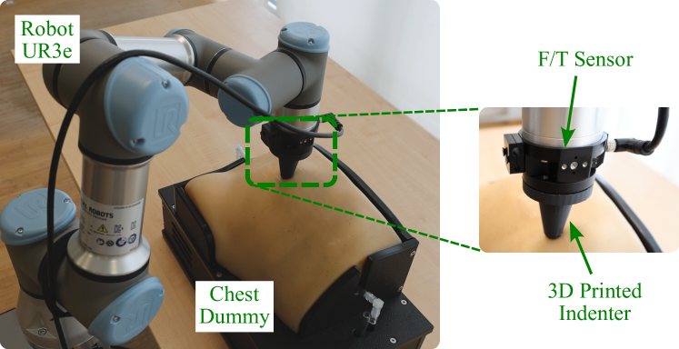
Figure 1: Experimental setup.

The performed experiments require the characterisation of the viscoelasticity map and the repetition of a proof-of-concept ultrasound in two conditions, namely with and without sudden patient motion. For each condition, we tested the two proposed variable impedance strategies (variable stiffness with constant force VS-CF and variable stiffness with variable force VS-VF) and we compared the results with an impedance control with constant stiffness (CS) and a force control with constant reference (CF).

The methodology is evaluated in a proof-of-concept robotic ultrasonography setup (Figure 1), made of a 6 DoFs position-controlled manipulator, the Universal Robot UR3e, a 6-axis F/T sensor, the BOTA System SensONE mounted at the robot’s end-effector, and a 3D-printed rigid conical indenter with a spherical tip ($2\text{\,}\mathrm{cm}$ radius, $7\text{\,}\mathrm{cm}$ height), which is used in the parameter estimation and in the controller evaluation to simulate the presence of the ultrasound probe. The UR3e is controlled by means of the Forward Dynamics Compliance Control (FDCC) [34], which unifies impedance, admittance and force control in a single strategy for position-controlled robots. To prevent potential patient harm and ensure experiment repeatability, we performed the sonography on a dummy chest, the Blue Phantom COVID-19 Lung Simulator ($$33\text{\,}\mathrm{cm}$\,\times\,$33\text{\,}\mathrm{cm}$\,\times\,$23\text{\,}\mathrm{cm}$$), which replicates the properties of human tissue, allowing clinicians to practice and develop the ultrasound imaging skills necessary to diagnose the key findings consistent, in this specific case, with COVID-19 cases. The anatomy of the device includes a lung, chest wall, ribs (1-5), and diaphragm. The viscoelastic map was computed with MATLAB 2023a, in particular exploiting lsqr for the least squares method, GRIDFIT [30] for the surface reconstruction, and fitrgp for the GPR. The QP problem was instead implemented in C++ using the open-source QPOASES solver [35] on Ubuntu 22.04. All experiments were run on a computer with an AMD Ryzen 9 5900X (24) @ 3.7 GHz $\times$ 12-cores CPU and 32 GB RAM.

III-A Viscoelastic Model Validation

Figure 2: Load tests obtained with the different models.

The standard procedure to evaluate a viscoelastic model is to perform a load and unload test at constant velocity. This test is done with a Cartesian position controller in the following way: the loading phase is done with constant velocity of $3\text{\,}\mathrm{c}\mathrm{m}\cdot\mathrm{s}^{-1}$ for $0.75\text{\,}\mathrm{s}$, the load is maintained then for $10\text{\,}\mathrm{s}$ to reach the equilibrium and finally there is the unloading phase with a velocity of $1.5\text{\,}\mathrm{c}\mathrm{m}\cdot\mathrm{s}^{-1}$ for $1.5\text{\,}\mathrm{s}$. Results of this test in Figure 2 show the limitation of the linear Kelvin-Voight, i.e., for the first phase of the penetration the model prediction is far from the measured force. The Hunt-Crossley model achieves better results in imitating how the body react under a load. Table I shows how the residual changes changing the value of $\beta$. Minimising its value over different points of the puppet we obtain that $\beta=1.35$ is the best compromise. This value of $\beta$ is used to estimate elasticity and viscosity of the tissue with the sinusoidal palpation and the least square method. A known issue of the least square method is that is crucial to have a large amount of observations in order to retrieve precise estimates. Figure 3 shows how the residuals are affected by the palpation time; after $5\text{\,}\mathrm{s}$ it appears a plateau so this time is taken as reference.

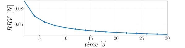
Figure 3: Variation of residual as palpation time changes.

The palpations on the chest dummy were made at a distance of $1\text{\,}\mathrm{cm}$ apart so that the surface could be accurately reconstructed. Figure 5 and Figure 4 show the results after the application of the GRIDFIT for the surface and of the GPR for the parameters of elasticity and viscosity.

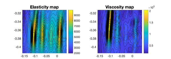
Figure 4: Resulting maps from the GPR computing the values of elasticity and viscosity every $0.1\text{\,}\mathrm{mm}$.

From Figure 5, it is possible to identify, starting from the left, the clavicle, the first rib, which is less stiff since it is under the pectoral muscle, the second, which is more stiff than the previous one but still under a layer of tissue, and the third, which is the stiffest because it is directly exposed.

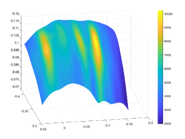
Figure 5: Surface reconstruction with elasticity information. The view is rotated of $180\text{\,}\mathrm{\SIUnitSymbolDegree}$ degrees wrt Figure 4 to better show the shape of the body.

TABLE I: Viscoelastic Model Validation

Relative Residual Value [N]
Kelvin-Voight	Hunt-Crossley
	$\beta$ = 1.5	$\beta$ = 1.35	$\beta$ = 1.1
0.066	0.029	0.014	0.045

III-B Variable Impedance Control Validation

Figure 6: Results of ultrasound experiment on a dummy chest in nominal conditions. (left) VS-CF, (right) VS-VF. The results of the CS and CF controllers are not reported here for the sake of space. A video of the experiments is available in the multimedia extension and in https://youtu.be/IwQhgzcd4IM.

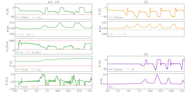
Figure 7: Comparison of ultrasound experiment on a dummy chest with disturbances: (a) VS-VF, (b) CS, (c) CF.

We compare the behaviour of the CF and CS controller against VS-CF and VS-VF that exploit the information of the body reconstruction. For simplicity, we assume the $\boldsymbol{K}^{d}$ to be diagonal as in [33]. During the experiments, the gains of the PD controller in [34] were set to $k_{p}=0.3$ and $k_{d}=0.01$ for all the controllers beside the CS where we let the default values of $k_{p}=0.05$ and $k_{d}=0.0005$ due to instability problems. For the experiments, a reference target is maintained at constant $z$ under the surface of the dummy to ensure the contact and is moved with constant velocity of $1\text{\,}\mathrm{c}\mathrm{m}\cdot\mathrm{s}^{-1}$ in the longitudinal direction of the chest dummy. Note that the force controller is hybrid since the $x$ and $y$ axes are controlled by the compliant controller, while the $z$ axis is controlled in force, hence it is not possible to give a reference value to this axis. As expected, the force generated by the CS control is strongly dependent from the shape of the body (Figure 7: when the surface is further from the target, the generated force is stronger than when the surface is closer. The force controller, instead, can track the target force without any problem but has the down side that can not be controlled in position, so it is not possible to rise the end-effector from the surface as in the case of the end of the experiment. Also, in case of problems, it would not be possible to stop the end effector except by resetting the target force it has to reach, which may result in dangerous motions. The VS-CF control can track a reference force as good as a force control (Figure 6), but without its downsides. It is possible in fact to control all the axes when in free motion and also suddenly detach the end-effector from the surface in case of necessity. On top, it uses the information registered by the reconstruction to cut the reference force when the maximum penetration is reached preventing the tip from sinking further. The VS-VF, instead of tracking a constant force, it is tracking the force necessary in order to keep a constant penetration into the material. In this case, the minimum force avoids to push too hard on the stiff points, such as the ribs: in fact, at these points, to achieve the desired penetration it would require more force than the maximum force we want to impart on the body.

The same test is done under the action of some disturbances to demonstrate the inherent safety of this new approach (Figure 7). Now the end-effector is pushed away from the surface to study how it would regain contact. Given that the safety of the approaches VS-CF and VS-VF is identical, indeed both use energy tanks and energy valves to avoid the creation of sudden forces, this test was done on one of them. We decide to choose the second one given that, in this approach, the maximum force is limited by a constant. Instead, in the first approach, the maximum force limit con be subject to estimation errors leaving room to possible dangerous behaviour. Figure 7 shows that, as soon as the end-effector starts to be moved away, the stiffness of the impedance spring start decreasing until no force is acting anymore; then, the spring value is limited to its minimum until the moment of the new contact. At the moment of contact, the stiffness would be inclined to increase suddenly but the presence of the valves partially limits its growth and restricts the tank from being emptied too quickly.

IV Conclusion

In this paper, we present a novel variable impedance strategy to regulate the interaction forces between the probe and the patient’s body in ultrasonography operations. The impedance parameters are obtained as a solution of a QP that accounts for the body’s biomechanics description and the controller’s passivity constraints. In particular, a parameter estimation procedure generates the viscoelastic map of the tissue, which in turn characterises softer and stiffer body parts. This is particularly useful in the case of lungs or heart ultrasounds, since the chest has bones (ribs) and muscles (intercostal, diaphagram). In addition, to ensure the stability of the variable impedance, the energy tank was used to observe the system passivity and prevent potential unsafe behaviours by limiting the maximum energy and the power flow. Experimental results show that the proposed controller outperforms the baseline in terms of tracking performance and safety. However, the approach has some limitations. First, the offline viscoelastic estimation requires the patient to not move during the exam, which is a weak hypothesis in our opinion. For this reason, we would like to perform an online parameter estimation while the exam is executed, as proposed by [36]. Second, proper motion tracking of the patient is required to match the viscoelastic model deformation as proposed in [8, 9]. In addition, tests on multiple human subjects will be performed.

References

- [1] European Reference Networks and Digital Health, “Market study on telemedicine,” European Commission, Tech. Rep., 2018. [Online]. Available: http://europa.eu
- [2] Digital Health and Innovation, “Consolidated telemedicine implementation guide,” World Health Organization, Tech. Rep., 2022. [Online]. Available: https://www.who.int/publications/i/item/9789240059184
- [3] S. Avgousti, E. G. Christoforou, A. S. Panayides, S. Voskarides, C. Novales, L. Nouaille, C. S. Pattichis, and P. Vieyres, “Medical telerobotic systems: current status and future trends,” BioMedical Engineering OnLine 2016 15:1, vol. 15, no. 1, pp. 1–44, 8 2016. [Online]. Available: https://biomedical-engineering-online.biomedcentral.com/articles/10.1186/s12938-016-0217-7
- [4] C. T. Coffin, “Work-related musculoskeletal disorders in sonographers: A review of causes and types of injury and best practices for reducing injury risk,” Reports in Medical Imaging, vol. 7, no. 1, pp. 15–26, 2014. [Online]. Available: http://dx.doi.org/10.2147/RMI.S34724
- [5] K. Li, Y. Xu, and M. Q. Meng, “An Overview of Systems and Techniques for Autonomous Robotic Ultrasound Acquisitions,” IEEE Transactions on Medical Robotics and Bionics, vol. 3, no. 2, pp. 510–524, 5 2021.
- [6] X. Ma, W. Y. Kuo, K. Yang, A. Rahaman, and H. K. Zhang, “A-SEE: Active-Sensing End-Effector Enabled Probe Self-Normal-Positioning for Robotic Ultrasound Imaging Applications,” IEEE Robotics and Automation Letters, vol. 7, no. 4, pp. 12 475–12 482, 10 2022.
- [7] J. Tan, Y. Li, B. Li, Y. Leng, J. Peng, J. Wu, B. Luo, X. Chen, Y. Rong, and C. Fu, “Automatic Generation of Autonomous Ultrasound Scanning Trajectory Based on 3-D Point Cloud,” IEEE Transactions on Medical Robotics and Bionics, vol. 4, no. 4, pp. 976–990, 11 2022.
- [8] C. Hennersperger, B. Fuerst, S. Virga, O. Zettinig, B. Frisch, T. Neff, and N. Navab, “Towards MRI-Based Autonomous Robotic US Acquisitions: A First Feasibility Study,” IEEE Transactions on Medical Imaging, vol. 36, no. 2, pp. 538–548, 2 2017.
- [9] J. Zhan, J. Cartucho, and S. Giannarou, “Autonomous Tissue Scanning under Free-Form Motion for Intraoperative Tissue Characterisation,” Proceedings - IEEE International Conference on Robotics and Automation, pp. 11 147–11 154, 5 2020.
- [10] M. C. Roshan, A. Pranata, and M. Isaksson, “Robotic Ultrasonography for Autonomous Non-Invasive Diagnosis - A Systematic Literature Review,” IEEE Transactions on Medical Robotics and Bionics, vol. 4, no. 4, pp. 863–874, 11 2022.
- [11] F. von Haxthausen, S. Böttger, D. Wulff, J. Hagenah, V. García-Vázquez, and S. Ipsen, “Medical Robotics for Ultrasound Imaging: Current Systems and Future Trends,” Current Robotics Reports 2021 2:1, vol. 2, no. 1, pp. 55–71, 2 2021. [Online]. Available: https://link.springer.com/article/10.1007/s43154-020-00037-y
- [12] Z. Jiang, S. E. Salcudean, and N. Navab, “Robotic ultrasound imaging: State-of-the-art and future perspectives,” Medical Image Analysis, vol. 89, p. 102878, 10 2023. [Online]. Available: https://linkinghub.elsevier.com/retrieve/pii/S136184152300138X
- [13] S. Merouche, L. Allard, E. Montagnon, G. Soulez, P. Bigras, and G. Cloutier, “A robotic ultrasound scanner for automatic vessel tracking and three-dimensional reconstruction of b-mode images,” IEEE Transactions on Ultrasonics, Ferroelectrics, and Frequency Control, vol. 63, no. 1, pp. 35–46, 1 2016.
- [14] R. Tsumura and H. Iwata, “Robotic fetal ultrasonography platform with a passive scan mechanism,” International Journal of Computer Assisted Radiology and Surgery, vol. 15, no. 8, pp. 1323–1333, 8 2020. [Online]. Available: https://link.springer.com/article/10.1007/s11548-020-02130-1
- [15] S. Virga, O. Zettinig, M. Esposito, K. Pfister, B. Frisch, T. Neff, N. Navab, and C. Hennersperger, “Automatic force-compliant robotic Ultrasound screening of abdominal aortic aneurysms,” IEEE International Conference on Intelligent Robots and Systems, vol. 2016-November, pp. 508–513, 11 2016.
- [16] A. Pappalardo, A. Albakri, C. Liu, L. Bascetta, E. De Momi, and P. Poignet, “Hunt–Crossley model based force control for minimally invasive robotic surgery,” Biomedical Signal Processing and Control, vol. 29, pp. 31–43, 8 2016.
- [17] M. Ferro, C. Gaz, M. Anzidei, and M. Vendittelli, “Online Needle-Tissue Interaction Model Identification for Force Feedback Enhancement in Robot-Assisted Interventional Procedures,” IEEE Transactions on Medical Robotics and Bionics, vol. 3, no. 4, pp. 936–947, 11 2021.
- [18] Z. Jiang, M. Grimm, M. Zhou, Y. Hu, J. Esteban, and N. Navab, “Automatic Force-Based Probe Positioning for Precise Robotic Ultrasound Acquisition,” IEEE Transactions on Industrial Electronics, vol. 68, no. 11, pp. 11 200–11 211, 11 2021.
- [19] J. Wang, C. Lu, Y. Lv, S. Yang, M. Zhang, and Y. Shen, “Task Space Compliant Control and Six-Dimensional Force Regulation Toward Automated Robotic Ultrasound Imaging,” IEEE Transactions on Automation Science and Engineering, 2023.
- [20] A. Duan, M. Victorova, J. Zhao, Y. Sun, Y. Zheng, and D. Navarro-Alarcon, “Ultrasound-Guided Assistive Robots for Scoliosis Assessment With Optimization-Based Control and Variable Impedance,” IEEE Robotics and Automation Letters, vol. 7, no. 3, pp. 8106–8113, 7 2022.
- [21] F. Ferraguti, N. Preda, A. Manurung, M. Bonfe, O. Lambercy, R. Gassert, R. Muradore, P. Fiorini, and C. Secchi, “An Energy Tank-Based Interactive Control Architecture for Autonomous and Teleoperated Robotic Surgery,” IEEE Transactions on Robotics, vol. 31, no. 5, pp. 1073–1088, 10 2015.
- [22] G. Raiola, C. A. Cardenas, T. S. Tadele, T. De Vries, and S. Stramigioli, “Development of a Safety- and Energy-Aware Impedance Controller for Collaborative Robots,” IEEE Robotics and Automation Letters, vol. 3, no. 2, pp. 1237–1244, 4 2018.
- [23] E. Shahriari, L. Johannsmeier, E. Jensen, and S. Haddadin, “Power Flow Regulation, Adaptation, and Learning for Intrinsically Robust Virtual Energy Tanks,” IEEE Robotics and Automation Letters, vol. 5, no. 1, pp. 211–218, 1 2020.
- [24] J. Lachner, F. Allmendinger, E. Hobert, N. Hogan, and S. Stramigioli, “Energy budgets for coordinate invariant robot control in physical human–robot interaction,” International Journal of Robotics Research, vol. 40, no. 8-9, pp. 968–985, 8 2021. [Online]. Available: https://journals.sagepub.com/doi/full/10.1177/02783649211011639
- [25] S. Hjorth, E. Lamon, D. Chrysostomou, and A. Ajoudani, “Design of an Energy-Aware Cartesian Impedance Controller for Collaborative Disassembly,” Proceedings - IEEE International Conference on Robotics and Automation, 2 2023. [Online]. Available: http://arxiv.org/abs/2302.03587
- [26] K. H. Hunt and F. R. Crossley, “Coefficient of Restitution Interpreted as Damping in Vibroimpact,” Journal of Applied Mechanics, vol. 42, no. 2, pp. 440–445, 6 1975. [Online]. Available: https://dx.doi.org/10.1115/1.3423596
- [27] N. Özkaya, M. Nordin, D. Goldsheyder, and D. Leger, “Fundamentals of biomechanics: Equilibrium, motion, and deformation: Third edition,” Fundamentals of Biomechanics: Equilibrium, Motion, and Deformation: Third Edition, pp. 1–275, 1 2012.
- [28] W. Flügge, Viscoelasticity. Berlin, Heidelberg: Springer Berlin Heidelberg, 1975. [Online]. Available: http://link.springer.com/10.1007/978-3-662-02276-4
- [29] N. Diolaiti, C. Melchiorri, and S. Stramigioli, “Contact impedance estimation for robotic systems,” IEEE Transactions on Robotics, vol. 21, no. 5, pp. 925–935, 10 2005.
- [30] J. D’Errico, “Surface fitting using gridfit,” MATLAB central file exchange, vol. 643, 2005.
- [31] C. K. Williams and C. E. Rasmussen, Gaussian processes for machine learning. MIT press Cambridge, MA, 2006.
- [32] P. Chalasani, L. Wang, R. Roy, N. Simaan, R. H. Taylor, and M. Kobilarov, “Concurrent nonparametric estimation of organ geometry and tissue stiffness using continuous adaptive palpation,” in Proceedings - IEEE International Conference on Robotics and Automation, vol. 2016-June, 2016.
- [33] J. Zhao, A. Giammarino, E. Lamon, J. Gandarias, E. Momi, and A. Ajoudani, “A Hybrid Learning and Optimization Framework to Achieve Physically Interactive Tasks With Mobile Manipulators,” IEEE Robotics and Automation Letters, vol. 7, no. 3, 2022.
- [34] S. Scherzinger, A. Roennau, and R. Dillmann, “Forward Dynamics Compliance Control (FDCC): A new approach to cartesian compliance for robotic manipulators,” IEEE International Conference on Intelligent Robots and Systems, vol. 2017-September, pp. 4568–4575, 12 2017.
- [35] H. Ferreau, C. Kirches, A. Potschka, H. Bock, and M. Diehl, “qpOASES: A parametric active-set algorithm for quadratic programming,” Mathematical Programming Computation, vol. 6, no. 4, pp. 327–363, 2014.
- [36] A. Haddadi and K. Hashtrudi-Zaad, “Real-time identification of hunt-crossley dynamic models of contact environments,” IEEE Transactions on Robotics, vol. 28, no. 3, pp. 555–566, 2012.