Faraday waves on a bubble Bose-Einstein condensed binary mixture

Abstract

By studying the dynamic stability of Bose-Einstein condensed binary mixtures trapped on the surface of an ideal two-dimensional spherical bubble, we show how the Rabi coupling between the species can modulate the interactions leading to parametric resonances. In this spherical geometry, the discrete unstable angular modes drive both phase separations and spatial patterns, with Faraday waves emerging and coexisting with an immiscible phase. Noticeable is the fact that, in the context of discrete kinetic energy spectrum, the only parameters to drive the emergence of Faraday waves are the $s-wave$ contact interactions and the Rabi coupling. Once analytical solutions for population dynamics are obtained, the stability of homogeneous miscible species is investigated through Bogoliubov-de Gennes and Floquet methods, with predictions being analysed by full numerical solutions applied to the corresponding time-dependent coupled formalism.

I Introduction

Spatial pattern formations can be observed in different branches of physics, whenever describing nonlinear wave propagations such as in fluids outside equilibrium and nonlinear optics 1993Cross . Indeed, surface wave excitations, which appear as patterns on liquids inside a vibrating receptacle, were first noticed and described by Faraday in 1831 1831Faraday , following his famous experiments on the formation of patterns in vibrating surfaces. The past few-decades progress achieved in reaching near-zero temperatures, allowing feasibility of Bose-Einstein condensates (BECs) in ultracold gases 1995Anderson ; 1995Davis ; 1995Bradley , together with new advanced techniques to control particle interactions, have opened new ways to explore and investigate how some well-known classical phenomena can stand and be realized in atomic trapped quantum fluids 1999Dalfovo ; 2016Stringari . In atomic gases, spatial patterns can be led by parametric modulations, with the emergence of Faraday waves been reported in several experimental and theoretical investigations 2002Staliunas ; 2007Engels ; 2010Nath ; 2016Sudharsan ; 2016Abdullaev ; 2019Abdullaev ; 2018Smits ; 2019Nguyen ; 2020Zhang ; 2020Maity ; 2021Kwon . Particularly concerned to theoretical activities on two-dimensional (2D) parametric instabilities in quantum gases, we have the recent work by Fujii et al. 2023Fujii , in which past and present studies can be traced from the references therein. With Faraday patterns in two-component superfluid, quite recently we had a report in 2022Cominotti on the observation of massless and massive collective excitations. Time-dependent modulations in trap potential or scattering length manipulations via Feshbach mechanisms 1999Feshbach are able to drive systems to target excited states 2020Brito , induce time-crystal formations 2019Zhu , manipulate population dynamics 1998Grifoni ; 2000Williams , as well as explore the Bardeen-Cooper-Schrieffer and BEC crossover, as recently reported in 2022He for bubble-trapped two-component atomic Fermi superfluid. On the actual possible technological applications related to manipulations of ultracold atoms in matter waves, the so-called atomtronics, we have a recent review in 2022Amico . In binary dipolar quantum gases, it was also demonstrated in 2020Turmanov the possibility to create persistent density waves, with Faraday instabilities generated by the population imbalance between the two hyperfine states. Another interesting way to induce Faraday waves was proposed in 2019Chen , considering interactions effectively modulated by the Rabi coupling between states. An effective interaction actually leads the dynamics2003Jenkins ; 2019Shibata , being able to trigger parametric resonances 1960Landau . Also applied by Raman-induced spin-orbit coupling 2022Zhang , this approach suggests some advantages in dealing with condensate mixtures.

Currently, condensate mixtures can be performed with the same atomic species initially set into different hyperfine states 1997Myatt , but also can be handled with different atomic species 2002Modugno . It is possible to study how one species is affected by the presence of another one 2021Alon . We can observe how the elementary excitations can grow and induce phase separation depending on the interaction parameters 2010Brtka ; 2021Andriati . An open question is how Faraday waves can be achieved in closed geometries, especially when the excitation is led by Rabi coupling. We turn our attention to bubble two-dimensional (2D) bubble shells in the spherical closed geometry, where the spectrum of elementary excitation is discrete, and therefore spatial patterns need very special conditions to be accomplished. Following previous theoretical investigations considering 2D shell-like potentials 2001Zobay ; 2004Zobay confining condensates in spherical and/or ellipsoidal surfaces, the recent particular interest is concerned to microgravity Bose gas experiments performed aboard the International Space Station 2020Aveline ; 2022Carollo ; 2023Lundblad , although bubble BEC has not yet been achieved in space. Looking for alternative closed 2D geometries, earth experiments have being reported on a shell bubble BEC produced by exploring the immiscibility of two species 2022Jia , as well as by controlling a quantum gas confined onto a shell-shaped surface Guo2022 . In this context, several related problems can be traced through recent works  2023Tononi ; 2018Padavic ; 2018Sun ; 2019Bereta ; 2019Tononi ; 2020Moller , in which fundamental properties can be found. More specifically, among others, we have studies on vortex dynamics and stability 2020Padavic ; 2021Andriati ; 2022Caracanhas ; 2023Saito , dipole interactions 2012Adhikari ; 2020Diniz , Berezinskii-Kosterlitz-Thouless transition 2022Tononi , thermodynamics properties 2019Pretipino ; 2021Rhyno , and bubble mixtures 2022Sturmer .

Our focus in the present work is on homogeneous condensates coupled by Rabi oscillations in a 2D spherical hollow shell. Inspired by results given in 2019Chen , we expect that the stability dynamics would be strongly affected by the Rabi coupling, triggering unstable modes, which can lead to the rising of new spatial patterns, eventually evolving to Faraday waves. In fact, our findings point out that, the Rabi oscillations are able to drive the condensates to states where the Faraday pattern coexists with an immiscible phase, where unstable modes are identified by the wave number. The same unstable angular modes which break a condensate into pieces 2021Andriati are able to induce Faraday-patterns excitations. We first study the stability dynamics by a comparative analysis of the elementary excitations spectrum obtained via the Bogoliubov-de Gennes (BdG) 2016Stringari method with the Floquet approach 1998Grifoni . Next, by performing the full dynamics with the corresponding Gross-Pitaevskii (GP) formalism, we observe that the Floquet approach is more suitable to study our coupled system than the BdG scheme, because the Floquet method takes into account dynamical effects which cannot be assimilated by the BdG approach. By tuning the Rabi coupling under given conditions, Faraday waves can emerge, persisting even in the immiscible phase.

The next sections are organized as follows. In Sect. II, we present the theoretical model for a Rabi-coupled two BEC mixture confined in the surface of a rigid spherical shell. The stability analyses are provided in Sects. III and  IV; by applying, respectively, the BdG approach to stationary solutions, and the Floquet method to homogeneous oscillating solutions. In Sect. V, the atom-population dynamics is performed by solving the full GP formalism, in which stability predictions are checked and we can observe the emergence of Faraday waves. Finally, in Sect. VI, we have our main conclusions with some perspectives. Among the four appendices with complementary material, particular attention should be given to Appendix B, which provides exact analytical solutions for binary density oscillations in a spherical bubble.

II Rabi-coupled BEC mixture on a rigid spherical shell

We consider a binary BEC mixture with two atomic species sharing the same mass $M$, which can be in two different hyperfine states. Our study is performed by assuming that both condensates are trapped on the surface of a rigid spherical shell, aiming to mimic the cold-atom bubble experiments currently performed in microgravity environments. For that, a reduction of the original three-dimensional (3D) GP coupled equation is performed to a corresponding two-dimensional (2D) formalism. The 2D approximation is reasonable as long as the radial excitations are inaccessible regarding the large amount of energy needed for it. This is true when the thickness $\delta R$ of the 3D spherical shell of radius $R$ is comparatively very small $(\delta R\ll R$), as extensively discussed in 2021Andriati . We also stress that our main concern is on the dynamic stability of the system, i.e., a context where we are not taking into account energetic instabilities, which could be triggered by a thermal cloud that is neglected here.

The condensates can be described in the mean-field approach as a system of two coupled GP equations 1999Dalfovo ; 2016Stringari , with atoms transferred from one state to the other by Rabi oscillations 2019Chen , by taking into account real Rabi coupling $\Omega$. With the total number of atoms $N$, the coupled condensates with respective populations are given by $N_{1}(t)$ and $N_{2}(t)$. They interact each other through their nonlinear two-body parameters $\overline{g}_{ij}\equiv 4\pi\hbar^{2}{a}_{ij}N/M$ ($i,j=1,2$), where $a_{jj}$ and $a_{12}=a_{21}$ are, respectively, the intra- and inter-species $s$-wave atom-atom scattering lengths. With this definition, we are assuming the total wave function normalized to 1, with each component $j=1,2$ normalized to $N_{j}(t)/N$. Along this paper, with exception of Appendix A, we use dimensionless variables and quantities, by taking the bubble radius $R$ as the length unit, with $\hbar^{2}/(MR^{2})$ and $MR^{2}/\hbar$ being the energy and time units, respectively. The dimensional reduction, from 3D to 2D, is detailed in the Appendix A, with the adimensionalization being explained at the end by factoring the energy unit. In this way, we end up with the following 2D coupled GP formalism describing each wave function $\Psi_{j}\equiv\Psi_{j}(\theta,\phi;t)$ normalized to $N_{j}$:

$${\rm i}\partial_{t}\Psi_{j=1,2} \!=\! -\frac{1}{2\sin\theta}\left[{\partial_{\theta}}\left(\sin\theta\,{\partial_{\theta}}\right)+\frac{1}{\sin\theta}{\partial_{\phi}^{2}}\right]\Psi_{j}$$ (1)

$$+ \sum_{i=1,2}g_{ji}{\left|\Psi_{i}\right|}^{2}\Psi_{j}+(-1)^{j}{\mathrm{i}}\Omega\Psi_{3-j},$$

where $\theta\in[0,\pi]$ and $\phi\in[0,2\pi]$ are, respectively, the usual polar and azimuthal angular positions in the sphere; and, the notation $\partial_{\chi}$ is being used for partial derivative of $\chi$. Also, represented in the 2D spherical surface, $g_{ij}=\frac{\sqrt{8\pi}a_{ij}N}{\delta R}$ (with $\delta R$ being the thickness of the bubble shell) are the nonlinear parameters for the inter- and intra-species interactions, derived in Appendix A from the original 3D formalism after factoring the energy unit . Our purpose is to study the stability of a miscible homogeneous system under different conditions, considering stationary as well as time-oscillating solutions.

The spatial part of (1) is directly proportional do the square of the angular momentum $\mathbf{L}$, given by ${\bf L}^{2}/(2\hbar^{2})$, with exact discrete $\ell-$state eigenvalues $\epsilon_{\ell}=\ell(\ell+1)/2$, corresponding to spherical harmonics eigenfunctions $Y_{\ell,m}(\theta,\phi)$. Therefore, it is appropriate to redefine the component wave functions for specific $\ell$ states as $\Psi_{j}(\theta,\phi;t)\equiv\psi_{j,\ell}(t)Y_{\ell,m}(\theta,\phi)$, such that, as $-\ell\leq m\leq\ell$, we can have $2\ell+1$ states with the same eigenvalue $\epsilon_{\ell}$. For convenience, the explicit time and $\ell$ labels will be removed within the redefinition $\psi_{j}\equiv\psi_{j,\ell}(t)$. In order to verify the time-dependent oscillatory behavior of $\psi_{j}$, let us assume the simplest case with $\Omega=0$, $N_{j}=N/2$, $g_{jj}=g$ and $g_{21}=g_{12}$, with the stationary-state wave functions identical for both components,

$$\psi^{(s)}_{j}=\sqrt{\frac{1}{8\pi}}\;\exp\left[{-{\mathrm{i}}\displaystyle\left(\frac{g+g_{12}}{8\pi}\right)}t\right],$$ (2)

where $(g+g_{12})/{(8\pi)}$ is the chemical potential. This stationary case can be easily extended to homogeneous periodic solutions, for $g_{12}=g$ and $\Omega\neq 0$. By including a time-dependent oscillating factor in the normalization, implying in periodic exchange of atoms between the species, the coupled wave functions are expressed by

$$\left(\begin{array}[]{l}\psi_{1}^{(0)}\\ \psi_{2}^{(0)}\end{array}\right)=\sqrt{\frac{1}{4\pi}}\left(\begin{array}[]{l}\cos\left(\Omega t+\frac{\pi}{4}\right)\\ \sin\left(\Omega t+\frac{\pi}{4}\right)\end{array}\right)\exp\left[{{-{\rm i}\left(\displaystyle\frac{g}{4\pi}\right)t}}\right].$$ (7)

The period of oscillations is given by $2\pi/\Omega$, which does not depend on the interactions, being twice the period for the densities $T_{0}\equiv\pi/\Omega$. For $\Omega\neq 0$ and $g_{12}\neq g$, a more general periodic solution of (1) can be derived, with

$$\psi_{j}(t)=f_{j}(t)\exp{(-{\mathrm{i}}\gamma_{j}t)},$$ (8)

where $f_{j}(t)$ are periodic complex functions (satisfying $|f_{j}(t+T)|^{2}=|f_{j}(t)|^{2}$ for a period $T$), with $\gamma_{j}$ being real and time-independent phases. An equivalent approach is to write $f_{j}(t)$ as real functions with time-dependent phases to be determined. By assuming both states equally populated at $t=0$, we have $|\psi_{j}(0)|^{2}={1/(8\pi)}$. The atom-number ratios of the two-atomic species, given by $N_{j}(t)/N=4\pi|\psi_{j}(t)|^{2}$, oscillate periodically within a cycle given by the period $T$ and amplitude ${\cal A}$ (maximum exchange number-ratio of particles), which in general are functions of the Rabi parameter $\Omega$ and nonlinear interactions $g_{ij}$. As shown for $g_{12}=g$, $T=T_{0}=\pi/\Omega$ does not depend on the interactions, with each density $|\psi^{(0)}_{j}(t)|^{2}$ oscillating between zero and $1/4\pi$. However, it can be shown that the period decreases as $|g-g_{12}|$ increases, with the maximum occurring when $g_{12}=g$ 2019Chen .

By considering Eq. (8) with $\Delta g\equiv(g_{12}-g)\neq 0$ and $\Omega\neq 0$, as shown in Appendix B, one can obtain the general solution, with time-dependent phases $\gamma_{j}$ not identical for both species [as verified in (60), where $\gamma_{j}$ is replaced by $\bar{\gamma}_{j}(t)$, the phases will depend on the respective densities $|\psi_{j}|^{2}$], . However, for the following stability analyses, we can consider they are carrying only the identical constant part, $\gamma_{1}=\gamma_{2}\equiv\gamma_{0}=(g+g_{12})/(8\pi)$, such that the time-dependent parcel of the phases are retained by the complex functions $f_{j}$, which in this case are satisfying

$$\partial_{tt}f_{j}+\left[\Omega^{2}+(\Delta g)^{2}\left(\frac{|f_{2}|^{2}-|f_{1}|^{2}}{2}\right)^{2}\right]f_{j}=0.$$ (9)

The derivation of the above, obtained from (1) with (8), follows analogously as shown in Appendix B, from (43) to (46). For $g_{12}=g$, this equation is identified with the harmonic oscillator equation having the frequency given by the Rabi parameter. The atom-ratio difference, which is defined by $\nu(t)\equiv\frac{N_{2}-N_{1}}{N}$ $=4\pi(|f_{2}|^{2}-|f_{1}|^{2})$ $=4\pi\left(|\psi_{2}|^{2}-|\psi_{1}|^{2}\right)$, satisfies the undamped unforced Duffing oscillator motion described by 2014Salas ; 2016Belendez ,

$$\partial_{tt}\nu+4\left[\Omega^{2}+\frac{1}{2}\left(\frac{\Delta g}{8\pi}\right)^{2}\nu^{2}\right]\nu=0,$$ (10)

which has exact solutions given by Jacobi elliptic periodic functions, for which the period is expressed by

$$T_{K}(\Omega,\alpha) = \frac{2}{\sqrt{{\Omega^{2}}+\alpha^{2}}}K\left(\frac{-\alpha^{2}}{\Omega^{2}+\alpha^{2}}\right),$$ (11)

$$\;{\rm with}\;\alpha \equiv {\left(\frac{{\cal A}\,\Delta g}{8\pi}\right)},$$ (12)

where ${\cal A}$ is the amplitude of the density difference $\nu$ oscillations, with $K(x)$ being the first-kind Jacobi elliptic function 2021Whittaker . For details, see Appendix B), where it was shown that this oscillating period is exact and can be obtained even before the explicit form of $\nu(t)$ is obtained. Here, for a convenient resemblance with the harmonic oscillator sinusoidal form, we assume $\nu(t)$ identified with

$$\nu(t) = {\cal A}\sin\left[2t\sqrt{\Omega^{2}+\frac{\alpha^{2}}{2}\left(\frac{\nu_{A}}{\cal A}\right)^{2}}\right],$$ (13)

where, for the moment, $\cal A$ and $\nu_{A}$ are parameters, which can be obtained from the exact solution of the Duffing equation. Within the present normalization of the coupled equation, ${\cal A}\leq 1$, being 1 for $(\Delta g)=0$. As derived in the Appendix B, constrained by the periodic conditions, $\cal A$ is a function of the ratio $(\Delta g)/\Omega$ given by

$$\frac{\cal A}{8\pi}={\sqrt{2}\frac{\Omega}{\Delta g}}\left[\sqrt{1+\left(\frac{\Delta g}{8\pi\Omega}\right)^{2}}-1\right]^{1/2}.$$ (14)

With the atom-ratio difference expressed by (13), the exchange oscillating time interval (from ${\cal A}$ to $-{\cal A}$), is one-half of the density period, given by

$$T=\frac{\pi}{\sqrt{\Omega^{2}+\frac{\alpha^{2}}{2}\left(\frac{\nu_{A}}{\cal A}\right)^{2}}},$$ (15)

which has an exact agreement with (12), for $\alpha=0$ ($\Delta g=0$), $K(0)={\pi}/2$. By matching (15) with (12) in the other extreme, $\Omega=0$ (the stationary limit), we obtain

$$\left(\frac{\nu_{A}}{\cal A}\right)=\left(\frac{\pi}{\sqrt{2}K(-1)}\right)=1.6945.$$ (16)

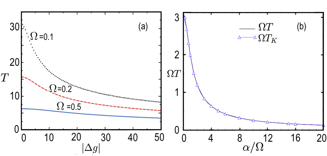
Figure 1: (Color online) In panel (a), the density oscillating period $T$ is given as a function of the absolute difference of the interaction parameters $|\Delta g|$, for three different Rabi couplings $\Omega$, as indicated. In panel (b), it is shown the perfect agreement between analytical expressions for the Duffing period $T_{K}$ (empty-triangles) and $T$ (solid-line), respectively multiplied by $\Omega$, given by (12) and (15), with $\alpha=\frac{{\cal A}\Delta g}{8\pi}$. Within defined units, all quantities are presented as dimensionless.

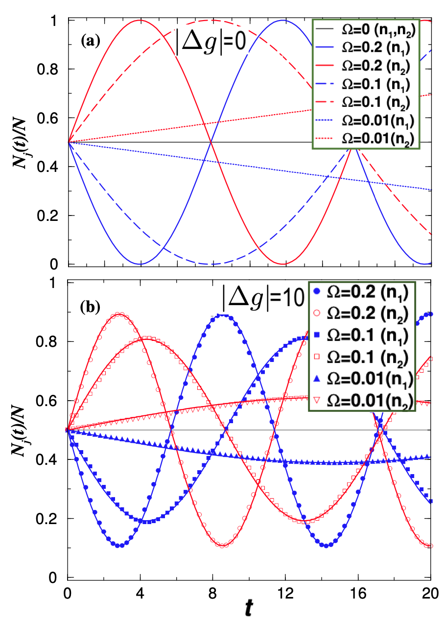
Figure 2: (Color online) Time-evolution of the atom-number ratio, $N_{j}(t)/N\equiv 4\pi|\psi_{j}(t)|^{2}\equiv 4\pi n_{j}$, with initial condition $N_{j}(0)=N/2$, for given Rabi couplings $\Omega$. In both panels, (a) for $|\Delta g|=0$, and (b) for $|\Delta g|=10$, the initially decreasing (increasing) lines refer to species 1 (species 2) [horizontal line for $\Omega=0$]. In (b), the full-numerical solutions (legend box), are matching with corresponding solid lines, given by (13), for $({\cal A},\Omega)=(0.7873,\;0.2)$, $(0.6261,\;0.1)$, and $(0.2214,\;0.01)$, with $(\nu_{A}/{\cal A})=\pi/\left(\sqrt{2}K(-1)\right)=1.6945$. Within defined units, all quantities are presented as dimensionless.

In Fig. 1, where we are displaying exact numerical results for the dependence of the oscillating period $T$ on the interaction difference $\Delta g$ for a few values of the Rabi frequency $\Omega$ [panel (a)], we also show the perfect agreement between the expressions (15) and (12) in panel (b). In panel (a), one can also notice explicitly how the oscillation period diminishes as the Rabi coupling increases.

To illustrate the density behavior, when considering different Rabi couplings and interactions, we also present two panels in Fig. 2, with few samples of full-numerical solutions for the corresponding density oscillations, together with close-approximated analytical solutions obtained by considering (9), as detailed in Appendix B. Panel (a) shows the behavior of the densities for the particular cases with $g_{12}=g$ when the two components follow the simple analytical expressions (7). In contrast, panel (b) illustrates the behavior of a more general case with $g_{12}\neq g$, according to Eq. (8), when the solutions are deviating from the simple sinusoidal form. For a given Rabi parameter $\Omega$, as the differences between the interactions ($|g-g_{12}|$) increase, the number of particles being exchanged (represented by the corresponding amplitudes) decreases, oscillating within a smaller interval. Correspondingly, also noticeable in Figs. 1-2, is the effect of symmetry breaking; when we broke the perfect balance between intra- and inter-species interactions the inter-condensate atom exchange frequency increases.

The perfect agreement between the expressions (15) and (12) is shown in Fig. 2(b), which implies that (13) is a close approximation to the exact solution of the Duffing equation. This fact is confirmed by some sample results shown in Fig. 2(b), where analytical results are compared with full numerical ones. From (13) both densities can be written as

$$|f_{j}(t)|^{2} = \frac{1}{8\pi}+(-)^{j}\frac{\cal A}{8\pi}\sin\left[2t\sqrt{\Omega^{2}+\frac{\alpha^{2}}{2}\left(\frac{\nu_{A}}{\cal A}\right)^{2}}\right],$$ (19)

$${\longrightarrow} \frac{1}{4\pi}\left\{\begin{array}[]{c}\cos^{2}(\Omega t)\\ \sin^{2}(\Omega t)\end{array}\right.\;{\rm for}\;\Delta g\to 0\;({\cal A}\to 1).$$

As the coupled system is normalized to one, with one density orthogonal to the other, the extremes for the difference are $\pm{\cal A}$, which happens when one of the species is at the maximum with the other at the minimum. When $\Omega\to 0$ (or $\Omega\ll|\Delta g|/(8\pi)$), we have the other extreme, with (19) satisfying the stationary case (2), with both densities being identical, $|f_{j}|^{2}=1/(8\pi)$. As $|\Delta g|$ increases, the periodic atom exchange between the coupled condensates decreases till reaching the stationary limit.

With respect to the Rabi frequency $\Omega$, more time is needed for an oscillating solution to complete each cycle with lower values of $\Omega$ than for higher ones. As verified in Fig. 2, for the initial time interval, lower frequencies provide almost linear behaviors (increasing or decreasing) with time when compared with the corresponding behavior obtained with higher frequencies. So, at short times, when the Rabi coupling is weak ($\Omega\rightarrow 0$), stationary solutions and oscillating ones are likely to be the same. This is no longer true for strong coupling.

III Bogoliubov-de Gennes stability analysis

The role of the Rabi coupling $\Omega$ on stationary solutions (2) is studied in this section by performing a dynamic stability analysis, using the BdG method 2010Brtka ; 2021Andriati . Within this approach, small amplitude oscillations are considered around the uniform stationary solution (7). With the perturbations being eigenfunctions of the kinetic energy operator, we can express the perturbed wave functions by $\ell-$angular-mode oscillations, in terms of the spherical harmonics $Y_{\ell,m}(\theta,\phi)$:

$$\psi_{j,\ell}^{(s)}(\theta,\phi;t)=\Big{\{}\sqrt{\frac{1}{8\pi}} + u_{j,\ell}^{(s)}Y_{\ell,m}(\theta,\phi){\mathrm{e}}^{-{\mathrm{i}}\omega_{\ell}t}$$ (20)

$$+ {v}_{j,\ell}^{(s)*}{Y}_{\ell,m}^{*}(\theta,\phi){\mathrm{e}}^{{\mathrm{i}}{\omega}_{\ell}^{*}t}\Big{\}}\mathrm{e}^{-{\mathrm{i}}\mu t},$$

where $u_{j,\ell}^{(s)}$ and $v_{j,\ell}^{(s)}$ are complex parameters to be determined. The spectral solutions are given by $\omega_{\ell}$, with $\ell$ being specific angular mode oscillations. Therefore, all the perturbation terms of (20) are exact solutions of the linear part of (1) 2021Andriati , with eigenvalues $\epsilon_{\ell}\equiv\ell(\ell+1)/2$. The particular simplified symmetric form of Eq. (1) allows us to assume perturbations with no dependence on the azimuthal mode excitation, given by $m$ (an integer running from $-\ell$ to $+\ell$), which can be arbitrarily chosen. Therefore, in the exponential factors of Eq. (20), the frequency parameters $\omega_{\ell}$ are excitation modes that carry only the angular momentum index $\ell$. They are in general complex numbers, with non-zero imaginary parts when the system becomes dynamically unstable. By initially assuming they are real numbers, we are considering parameters such that the system is in a stable configuration. As we vary these parameters, for some specific modes of oscillation the system becomes unstable, acquiring non-zero imaginary parts.

By inserting the perturbation (20) into the Eq. (1), neglecting the second and higher-order amplitude terms, we obtain the corresponding BdG matrix equation,

$$\left[{\mathbf{M}^{(s)}}-\omega_{\ell}\right]{\mathbf{u}}_{\ell}^{(s)}=0,$$ (21)

where $\bf M^{(s)}$ contains the model parameters $g_{ij}$ and $\Omega$,

$${\mathbf{M}^{(s)}}=\begin{bmatrix}\epsilon_{\ell}+\frac{g}{8\pi}&\frac{g}{8\pi}&\frac{g_{12}}{8\pi}-{\mathrm{i}}\Omega&\frac{g_{12}}{8\pi}\\ -\frac{g}{8\pi}&-\epsilon_{\ell}-\frac{g}{8\pi}&-\frac{g_{12}}{8\pi}&-\frac{g_{12}}{8\pi}-{\mathrm{i}}\Omega\\ \frac{g_{12}}{8\pi}+{\mathrm{i}}\Omega&\frac{g_{12}}{8\pi}&\epsilon_{\ell}+\frac{g}{8\pi}&\frac{g}{8\pi}\\ -\frac{g_{12}}{8\pi}&-\frac{g_{12}}{8\pi}+{\mathrm{i}}\Omega&-\frac{g}{8\pi}&-\epsilon_{\ell}-\frac{g}{8\pi}\end{bmatrix},$$ (22)

and ${\mathbf{u}}_{\ell}^{(s)}$ is the column vector defined by the perturbed amplitudes in (20), with transpose $\Big{[}u_{1,\ell}^{(s)}\ v_{1,\ell}^{(s)}\ u_{2,\ell}^{(s)}\ v_{2,\ell}^{(s)}\Big{]}^{\rm T}$. By solving the corresponding determinant, four possible solutions for each $\ell$ mode are obtained, given by

$$\omega_{\ell,\pm}^{2}\!\! = \!\!\left(\epsilon_{\ell}^{2}+\frac{\epsilon_{\ell}\;g}{4\pi}\right)+\Omega^{2}\pm 2\sqrt{\left(\epsilon_{\ell}^{2}+\frac{\epsilon_{\ell}\;g}{4\pi}\right)\Omega^{2}+\frac{\epsilon_{\ell}^{2}\;g_{12}^{2}}{(8\pi)^{2}}}.$$ (23)

However, two of them with opposite overall signs are redundant as they correspond to exchanging signals in the original definitions, such that only the positive ones will be considered. The system is said to be dynamically stable if these frequencies are real: $\mathrm{Im}(\omega_{\ell,\pm})=0$; becoming dynamically unstable when some of the solutions became complex: $\mathrm{Im}(\omega_{\ell,\pm})\neq 0$.

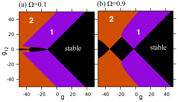
Figure 3: (Color online) BdG stability diagrams for the interaction parameters $g_{12}$ vs $g$, as given by (23). Stable regions [Im($\omega_{\ell,\pm}$) = 0] are represented in black, with unstable $\ell-$modes [Im$(\omega_{\ell,\pm})$ $\neq 0$] (with $\ell$ values indicated inside the regions) are in colors [violet for $\ell=1$ and orange for $\ell=2$]. The Rabi coupling $\Omega=0.1,0.9$ are indicated at the top of the respective panels. Within defined units, all quantities are presented as dimensionless.

In Fig. 3, we present a BdG stability diagram, which depicts how large is the stable region as one varies the interactions. By comparing the panels 3(a) and 3(b), we verify that the Rabi strength has an important role in rising new stability regions.

IV Floquet stability analysis

Let us now consider the evolution of the system given by the homogeneous oscillating solutions (8), under small amplitude oscillations, in order to better take into account the role of Rabi coupling in the dynamics. For that, we can study the solutions dynamically by the time-dependent Floquet method 2019Chen ; 2022Zhang , using small amplitude oscillations. For the present Floquet stability analysis, we are considering that the phases of the wave-function component $\psi_{j}(\theta,\phi;t)$ have a common time-independent part given by $\gamma_{j}=\gamma=(g+g_{12})/(8\pi)$, with $f_{j}(t)$ being complex, carrying any other relevant part of the phases. Another equivalent approach, with time-dependent phases $\gamma_{j}$ and real $f_{j}(t)$, is detailed in the Appendix B. In this case, by applying small amplitude oscillations in (8), we have

$$\psi_{j}(\theta,\phi;t) = f_{j}(t)\exp\left({-{\mathrm{i}}\gamma t}\right)$$

$$+ \left[{u}_{j,\ell}Y_{\ell,m}(\theta,\phi)+{v}_{j,\ell}^{*}Y^{*}_{\ell,m}(\theta,\phi)\right]{\rm e}^{-{\rm i}\gamma t},$$

where the amplitudes ${u}_{j,\ell}\equiv{u}_{j,\ell}(t)$ and ${v}_{j,\ell}\equiv{v}_{j,\ell}(t)$ are periodic time-dependent functions, with the same period $T$ as $f_{j}$, such that $|\psi_{j}(t+T)|^{2}=|\psi_{j}(t)|^{2}$. By inserting (IV) into (1), neglecting the second and higher-order terms, we get the following matrix equation 2019Chen :

$${\mathrm{i}}\frac{d}{dt}\!\!\left[\begin{array}[]{c}{u}_{1,\ell}\\ {v}_{1,\ell}\\ {u}_{2,\ell}\\ {v}_{2,\ell}\end{array}\right]\!\!=\!\!\begin{bmatrix}{D}_{1}&&G_{11}&&D_{12}&&G_{12}\\ -G_{11}^{*}&&-{D}_{1}&&-G_{12}^{*}&&-D_{12}^{*}\\ D_{12}^{*}&&G_{12}&&{D}_{2}&&G_{22}\\ -G_{12}^{*}&&-D_{12}&&-G_{22}^{*}&&-{D}_{2}\end{bmatrix}\!\!\left[\begin{array}[]{c}{u}_{1,\ell}\\ {v}_{1,\ell}\\ {u}_{2,\ell}\\ {v}_{2,\ell}\end{array}\right]\!\!,$$ (33)

where the elements are ${D}_{j}\equiv(\epsilon_{\ell}-\gamma)+2g{|f_{j}|}^{2}+g_{12}{|f_{3-j}|}^{2}$, $D_{12}\equiv g_{12}f_{1}f_{2}^{*}-{\rm i}\Omega$, and $G_{ij}\equiv g_{ij}f_{i}f_{j}$ ($g_{jj}=g$). When the system is driven by a periodic time-dependent Hamiltonian, the Floquet theorem 1998Grifoni predicts that the solutions ${{\mathbf{u}}}_{\ell}(t)$ can be written as

$${\mathbf{u}}_{\ell}(t)=\exp{({\lambda}_{\ell}t)}{\mathbf{p}}_{\ell}(t),$$ (34)

where ${\mathbf{p}}_{\ell}$ are periodic functions, which in our case satisfy the same periodicity of the densities. The factor $\lambda_{\ell}$ stands for the Floquet exponent. From its periodic property at the time $t=T$, ${\mathbf{p}}_{\ell}(T)={\mathbf{p}}_{\ell}(0)$, we obtain

$${\mathbf{u}}_{\ell}(T)=\exp{(\lambda_{\ell}T)}{\mathbf{p}}_{\ell}(0).$$ (35)

Numerical approach: Our approach to performing the Floquet stability analysis relies on an exact numerical calculation of the relevant observables. An analytical approach to obtain the associated wave functions with their small oscillating amplitudes can only be done at some approximate level (as discussed in Sec. II and Appendix B). Therefore, for practical purposes, we follow a method similar to 2019Chen , by integrating the Eq. (33) using a fourth-order Runge-Kutta method (RK4) from $t=0$ to $t=T$ (a complete period), assuming four different initial conditions for the amplitudes, which are ${\mathbf{u}}_{\ell}(0)=$ $[1\ 0\ 0\ 0]^{\rm T}$, $[0\ 1\ 0\ 0]^{\rm T}$, $[0\ 0\ 1\ 0]^{\rm T}$, and $[0\ 0\ 0\ 1]^{\rm T}$, being the four column vectors of a matrix ${\mathbf{F}}$, that at $t=0$ is the identity matrix ${\mathbf{F}}(t=0)=[{\mathbf{u}}_{\ell}^{(1)}(0)\ {\mathbf{u}}_{\ell}^{(2)}(0)\ {\mathbf{u}}_{\ell}^{(3)}(0)\ {\mathbf{u}}_{\ell}^{(4)}(0)]={\mathbf{I}}$. Separately, each initial condition vector will correspond to a different vector at $t=T$, that will define the evolved matrix as ${\mathbf{F}}(t=T)=[{\mathbf{u}}_{\ell}^{(1)}(T)\ {\mathbf{u}}_{\ell}^{(2)}(T)\ {\mathbf{u}}_{\ell}^{(3)}(T)\ {\mathbf{u}}_{\ell}^{(4)}(T)]$. By considering the eigenvalues of ${\mathbf{F}}$ given by $F_{\lambda_{\ell}}$, and once identified the matrix with (35), we are able to obtain the Floquet exponent as $\lambda_{\ell}=\ln(F_{\lambda_{\ell}})/T$. If the system evolves to the time $t=T$ with nonzero real part in the full spectrum having $(\lambda_{\ell}^{R})>0$, it implies that solution ${\mathbf{u}}_{\ell}$ is growing exponentially with $t$ for that specific mode $\ell$, being no longer stable. In other words, the uniform oscillating system is dynamically unstable under that $\ell$ orbital excitation. By using this approach, we are also able to study how far the BdG approach returns consistent results. As known, the BdG stability method is suitable for stationary solutions. However, when the system is under fast Rabi oscillations, the Floquet approach can give us more reliable results, which can indicate the level of disagreement with results obtained by the BdG method. In the Appendix C, we provide a more detailed comparison between both methods.

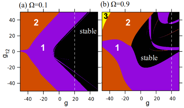
Figure 4: (Color online) Floquet stability diagrams for constant couplings, $\Omega=0.1$ (a) and $\Omega=0.9$ (b), parametrized by the interactions $g_{12}$ vs $g$, determined by $(\lambda_{\ell}^{R})_{\rm max}$ [See (33)-(35)]. The stable regions [$(\lambda_{\ell}^{R})_{\rm max}\leq 0$] are in black, with unstable ones [$(\lambda_{\ell}^{R})_{\rm max}>0$] having the $\ell-$mode given in colors [violet ($\ell=1$), orange ($\ell=2$) and yellow ($\ell=3$)]. The dashed lines, at $g=20$ (a) and $g=40$ (b) refer to results presented, respectively, in (a) and (b) of Fig. 5. Within defined units, all quantities are presented as dimensionless.

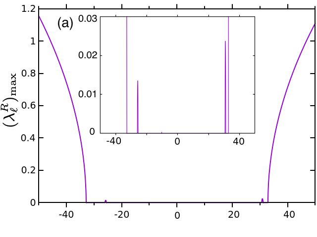
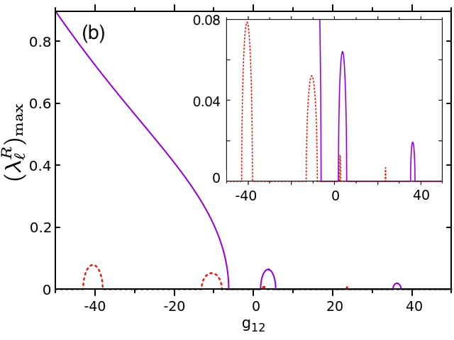
Figure 5: (Color online) Floquet spectra, given by $(\lambda_{\ell}^{R})_{\rm max}$, from (35), are shown as functions of the inter-species interaction $g_{12}$, with the intra-species and Rabi coupling parameters fixed at ($\Omega$, $g$)$=$ (0.1, 20) (a) and (0.9, 40) (b). The $\ell=$1 and 2 unstable modes are, respectively, represented by solid-violet and dashed-orange lines. In the insets,$(\lambda_{\ell}^{R})_{\rm max}$ is re-scaled to improve visibitily of lower peak instability regions. Within defined units, all quantities are presented as dimensionless.

Figure 4 displays two panels with Floquet stability diagrams, parametrized by the intra- and inter-species interactions, obtained from the oscillating functions $f_{j}$ for a complete period $T$. In panel (a), we choose a small value for $\Omega=0.1$, that provides good agreement with the stationary results presented in panel (a) of Fig. 3. As shown in panel (b), the agreement is no more maintained when considering a large value $\Omega=0.9$ for the Rabi constant, as compared with panel (b) of Fig. 3. In these diagrams, the dominant unstable angular modes $\ell=1,2,3$ are indicated inside the panels. Besides the similarity between the diagrams (a) of Figs. 3 and 4, for $\Omega=0.1$, the corresponding diagrams are already useful to verify the effect of more detailed stability analysis. As noticed, some stable regions verified with the BdG approach are no more confirmed when using the Floquet method, such as the regions with $g<0$, near $g_{12}=0$. Even for $g>0$, in the dominantly stable regions pointed out by the BdG approach, we can already verify instabilities detected by the Floquet method. Particularly, the border of the regions can no longer be kept when we carry out a more accurate stability study. These results, together with the following ones that we are going to discuss, led to the conclusion that, as soon as the Rabi coupling is turned on, the Floquet method is more sensible to system instabilities as one varies the inter- and intra-species interactions, being more accurate in studying the stability of a system than the conventional stationary BdG approach.

In the two panels of Fig. 5, we select two sets of parameters from the Floquet diagrams shown in Fig. 4, for separate representation of the corresponding spectra, given by the maximum of the real part of the Floquet exponent, $(\lambda_{\ell}^{R})_{\rm max}$. The two panels are representing the respective spectrum in terms of the inter-species interaction $g_{12}$ by considering fixed values of intra-species interactions and Rabi frequencies, with ($\Omega$, $g$)= (0.1, 20) in panel (a) and (0.9, 40) in panel (b). Figure 5, with the spectrum of unstable modes, is also indicating the meaning of the very faint lines appearing in the two diagrams of Fig. 4. In these two cases, we have only unstable modes with $\ell=$ 1 (solid-violet lines) and 2 (dashed-orange lines), as indicated. The respective insets in both panels are displayed to enhance the visibility of the lower peaks observed in the larger panels. The Floquet spectrum is also able to predict the existence of resonant conditions that can happen according to the chosen parameters. The conditions for that will be discussed in the next section IV.1, where a comparison is provided with a semi-analytic model when $|\Delta g|/(8\pi)\ll\Omega$.

IV.1 Resonance Conditions

It is possible to figure out the excitation mechanism responsible for the observed Floquet unstable spectrum by analyzing the resonance conditions, as discussed in Ref. 2019Chen . Our approach mainly differs from this reference when considering the free-particle spectrum in the formalism, as in our case the full kinetic energy term is provided by the squared angular momentum operator. Therefore, the continuum $\epsilon_{k}$ must be replaced by the corresponding discrete angular spectrum $\epsilon_{\ell}$. So, with the assumption that $|\Delta g|\ll 8\pi\Omega$, by using a first-order approximation in $\Delta g$ with slight corrections in the solutions in Eq. (7), valid in the regime $g_{12}=g$, we are able to get linearized equations (See Appendix D), with two natural frequencies as obtained from (66). In the limit $|\Delta g|=|g_{12}-g|\ll 8\pi\epsilon_{\ell}$, they are

$$\omega_{d,\ell}\approx\sqrt{\epsilon_{\ell}\left(\epsilon_{\ell}+\frac{g}{2\pi}\right)}+\frac{\sqrt{\epsilon_{\ell}}\Delta g}{16\pi\sqrt{{\epsilon_{\ell}+\frac{g}{2\pi}}}},$$ (36a)

$$\omega_{s,\ell}\approx\epsilon_{\ell}+\frac{\Delta g}{16\pi}.$$ (36b)

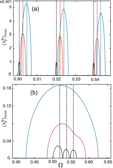
Figure 6: (Color online) Unstable Floquet spectra [$(\lambda_{\ell}^{R})_{\rm max}$], for $\ell=1$ with different $\Delta g$, are shown as functions of the coupling $\Omega$. In (a), the results are for $\Delta g=$ 0.1 (the three black curves with maxima near 0.001), 0.3 (the three red curves with maxima near 0.003), and 0.5 (the three blue curves with maxima higher than 0.004). In (b), we consider higher $\Delta g$ values, with $\Delta g=$ 2.0 (the three black curves with maxima below 0.03), 4.0 (the single red curve with a maximum near 0.08), and 7.0 (the larger single blue curve with a maximum near 0.17). The dashed vertical lines, obtained from (37), are pointing out the corresponding predictions, which are very close to the respective maxima, in (a). However, in (b), the close agreement happens only for $\Delta g=$ 2.0, as shown. Within defined units, all quantities are presented as dimensionless.

Parametric resonances are achieved when an external potential go with about twice the natural frequencies of the system 1960Landau . Once the $\ell$-mode excitations evolve in time with $\cos(4\Omega_{\ell}t)$ and $\sin(4\Omega_{\ell}t)$ 2019Chen , three critical couplings $\Omega_{\ell}$ emerge, which can be tuned to trigger the resonances

$${\Omega}_{\ell}^{(1)}=\frac{\omega_{d,\ell}}{2},\;\;{\Omega}_{\ell}^{(2)}=\frac{\omega_{s,\ell}}{2},\;\;{\Omega}_{\ell}^{(3)}=\frac{\omega_{d,\ell}+\omega_{s,\ell}}{4},$$ (37)

which are usually associated with density-density, spin-spin, and density-spin resonances, respectively 2019Chen . For the limit $g=0$, one can clearly see that the three resonant peaks are going to merge in just one peak, $(1/2)\left({\epsilon_{\ell}}+\frac{g_{12}}{16\pi}\right)$. These resonant positions can be observed in the Floquet spectrum in the regime of $g_{12}\approx g$. When $g_{12}$ becomes higher, the three peaks continuously merge into only one peak. In Fig. 6, we compare the Floquet spectrum with the approximations given by (37) for the resonance couplings. As seen in panel (a), for $\Delta g=$0.1, 0.3, and 0.5, the predicted values match exactly with the resonance peaks. In panel (b), the three-peak predictions are shown only for $\Delta g=$2.0, which are close to the exact numerical solutions. In the other two cases, with $\Delta g=$ 4 and 7, as the predictions are no more valid, we include only the numerical exact solutions presenting the corresponding single maxima.

V Atom-population dynamics

The dynamics of the atom-population exchange for the system was done by full numeric calculations of the coupled GP Eqs. (1), carrying out the spectral method introduced in Ref. 2021Andriati . Within our numerical computation, the dynamics is performed with time steps $\Delta t=10^{-5}$, having spatial grids, in $\theta$ and $\phi$ directions, with range sizes of $256\times 256$ and respective step sizes given by $\Delta\theta=\pi/256\approx 0.013$ and $\Delta\phi=2\pi/256\approx 0.025$. The GP equations are solved by starting with homogeneous solutions in which each species has half of the total population, i.e, $\psi_{1}=\psi_{2}=1/\sqrt{8\pi}$, with a $5\%$ random noise added to each point in the mesh grid. In this numerical approach, we are able to verify how long the homogeneous periodic solutions (8) solved by using the RK4 method provide a good model to describe the evolution of the populations. The stability behavior of the homogeneous miscible initial states is observed by displaying their overlap evolution, population dynamics, and density pattern when unstable modes occur.

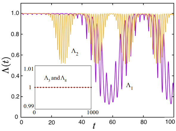
Figure 7: (Color online) Time-evolution of density overlaps, $\Lambda(t)$, from (38), for the coupling and set interactions ($\Omega,g,g_{12}$) given by: $\Lambda_{1}$ (0.50, 1, 8), $\Lambda_{2}$ (0.94, 40, -10), $\Lambda_{3}$ (0.10, 1, 10), and $\Lambda_{4}$ (0.99, 1, 25). $\Lambda_{1}$ and $\Lambda_{2}$ (main panel) are identified by solid-violet and solid-orange lines. The stability of $\Lambda_{3,4}$ is shown in the inset. Within defined units, all quantities are presented as dimensionless.

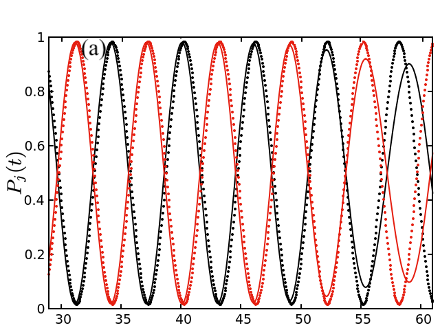
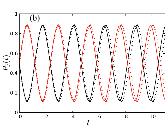
Figure 8: (Color online) The population time-evolution $P_{j}(t)$, given by (39), is shown for the Rabi and interaction parameters ($\Omega$, $g$, $g_{12}$) = (0.50, 1, 8) (a) and (0.94, 40, -10) (b), respectively. Solid lines stand for the full GP computation of (1), which takes into account the spatial-time-dependent wave functions, with the dotted ones for the homogeneous only time-dependent solutions (8). The colors, black and red, are identifying, respectively, species 1 and 2. The amplitudes agree with (14), being ${\cal A}=0.9657$, for $\Delta g=7$; and ${\cal A}=0.7737$, for $\Delta g=50$. Within defined units, all quantities are presented as dimensionless.

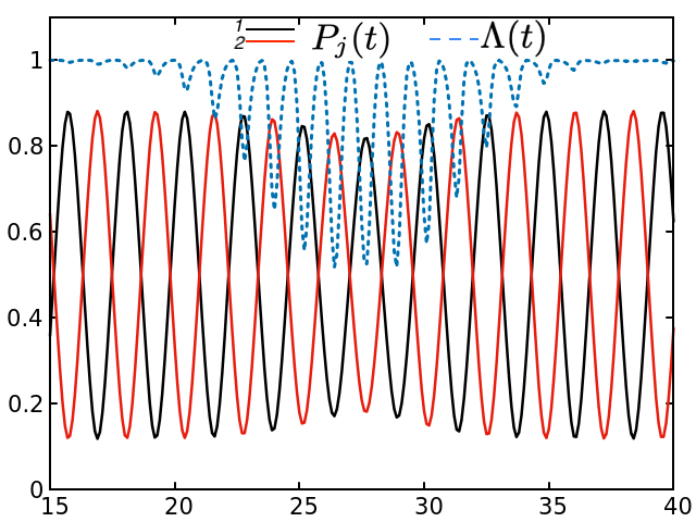
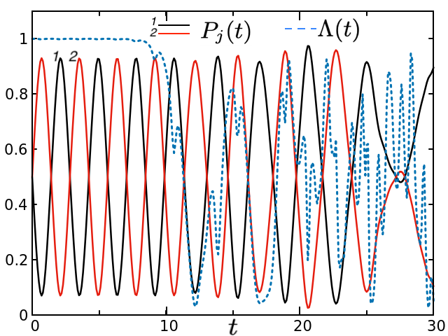
Figure 9: (Color online) Time-evolution of populations, $P_{j}(t)$ (solid lines) and overlaps, $\Lambda(t)$ (dashed-blue lines), as given by (39) and (38),respectively. Species 1 and 2 populations are given by solid lines (black and red, respectively), as indicated. The Rabi and interaction parameters are ($\Omega$, $g$, $g_{12}$) = (0.94, 40, -10) in (a); and (0.90, -10, 20), in (b). Within defined units, all quantities are presented as dimensionless.

To estimate the miscibility of the system, the overlap of densities are verified by the parameter $\Lambda$, defined by

$$\Lambda(t)=\frac{{\left[\int d\phi\sin\theta d\theta{|\psi_{1}|}^{2}{|\psi_{2}|}^{2}\right]}^{2}}{\left[\int d\phi\sin\theta d\theta{|\psi_{1}|}^{4}\right]\left[\int d\phi\sin\theta d\theta{|\psi_{2}|}^{4}\right]}.$$ (38)

When $\Lambda=1$, the species are miscible, while $\Lambda<1$ stands for immiscible condensates. Once the initial overlap decreases, it means that the initial miscible setup is no longer stable. In Fig. 7, we show the overlap dynamics regarding four different set of parameters, where the set of parameters including intra- and inter-species interaction, and Rabi coupling constant are given by ($\Omega$, $g$, $g_{12}$)=(0.50, 1, 8), (0.94, 40, -10), (0.10, 1, 10), and (0.99, 1, 25), for which the stability predictions can be localized in Figs. 13(b), 15 , 4(a) and 13(c), respectively. A complementary analysis can be made by observing the population dynamics of the previous cases, with the population $P_{j}$ of each species given by

$$P_{j}(t)=\frac{\int d\phi\sin\theta d\theta\ {|\psi_{j}|}^{2}}{\int d\phi\sin\theta d\theta\ \left[|\psi_{1}|^{2}+|\psi_{2}|^{2}\right]}=\frac{N_{j}(t)}{N}.$$ (39)

Figure 8 shows how the population oscillation is affected when the system becomes unstable. The population behavior is closely related to the overlap since both properties are changed when the miscible homogeneous initial ansatz (8) are no longer the true solutions of the system. It is important to note that the overlap dynamics for unstable cases are driven by two different frequencies. The slow frequency is a periodic behavior of miscibility, which was first observed in our previous work 2021Andriati , and it happens only for specific choices for interaction parameters. Moreover, in this work, we observe a second frequency in the overlap dynamics, which is faster than the first one, and is driven by the population dynamics frequency. In Fig. 9, we present two different sets of parameters where both frequencies are actually leading the overlap behavior. In panel 9(a), which refers to ($\Omega$, $g$, $g_{12}$) = (0.94, 40, -10), we clearly see that the faster kind of overlap oscillation has the same frequency as the population dynamics. Another set of parameters is depicted in panel 9(b), with ($\Omega$, $g$, $g_{12}$) = (0.90, -10, 20), for which we have the stability prediction in Fig. 4(b). Here, observing some periodic behavior with two distinguished frequencies is not as direct as in the previous case. This is an example where slower kind of modulation is not periodic, as also being observed 2021Andriati . In this way, the periodic oscillation caused by the Rabi coupling can be expected for all choices of parameters, but the same statement is not true for slower kind of modulation.

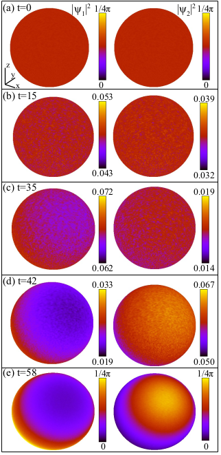
Figure 10: (Color online) Dynamics of densities ${|\psi_{1}|}^{2}$ (left column) and ${|\psi_{2}|}^{2}$ (right column), for the species $j=1$ and 2, considering the Rabi and interactions given by ($\Omega$, $g$, $g_{12}$) = (0.50, 1, 8). The time snapshots $t$ are indicated inside respective pair of panels, with density variations, according to (19) and (14), being within the interval $[0.0014\leq|\psi_{j}|^{2}\leq 0.0782$. At any $t$, $\sum_{j}|\psi_{j}|^{2}={1}/{(4\pi)}$, with identical $|\psi_{j}|^{2}=1/(8\pi)$ at $t=0$ and at each half period $T/2$. Within defined units, all quantities are presented as dimensionless.

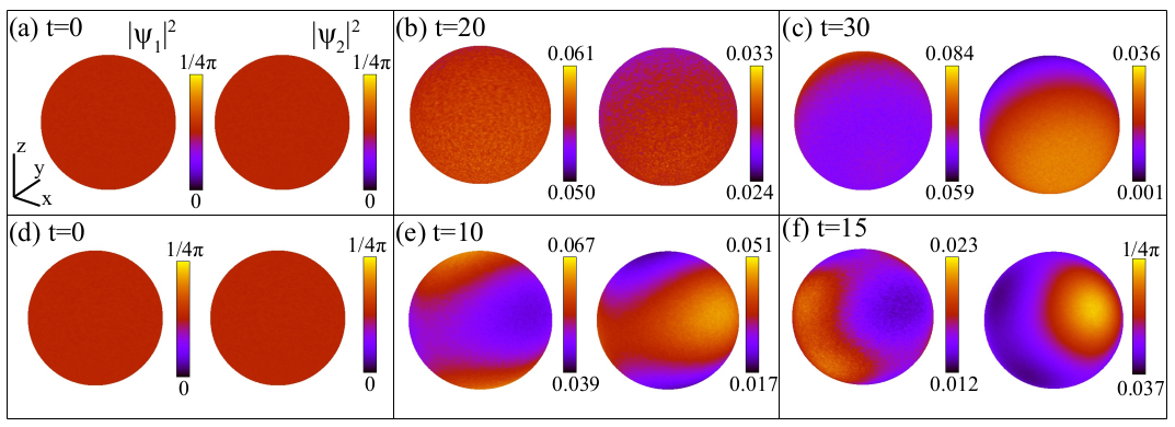
Figure 11: (Color online) Dynamics of densities ${|\psi_{j}|}^{2}$ for the parameters ($\Omega$, $g$, $g_{12}$) = (0.94, 40, -10) [upper panels, with $t$ = 0 (a), 20 (b), and 30 (c)], and (0.9, -10, 20) [lower panels, with $t$ = 0 (d), 10 (e), and 15 (f)]. The range of densities in the upper and lower panels are, respectively, $[0.01388\leq|\psi_{j}|^{2}\leq 0.06569]$ and $[0.00529\leq|\psi_{j}|^{2}\leq 0.07428]$. For each pair, the densities $|\psi_{j}|^{2}$ are given as indicated inside panel (a). Within defined units, all quantities are presented as dimensionless.

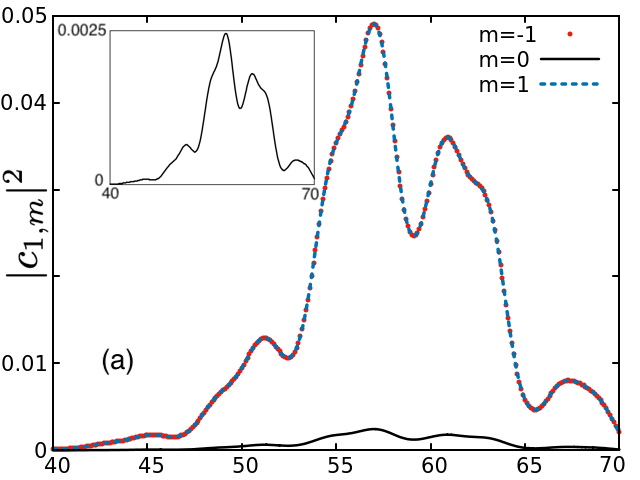
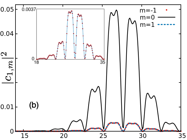
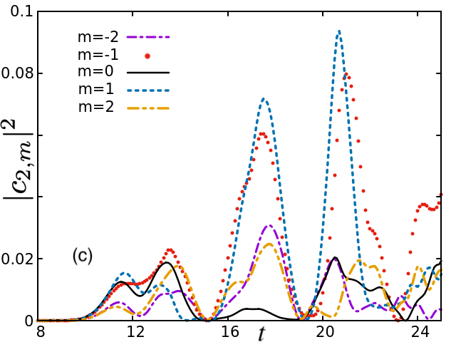
Figure 12: (Color online) Time evolution of couplings ${|c_{\ell,m}(t)|}^{2}$ for the species 1 [see (40)], for three unstable different set of parameters ($\Omega$, $g$, $g_{12}$) = (0.50, 1, 8), (0.94, 40, -10), and (0.90, -10, 20), which are depicted in (a), (b), and (c), respectively. The insets in (a) and (b) stand for the lower lines shown in the main panels. Within defined units, all quantities are presented as dimensionless.

The dynamics due to an unstable mode driving the behavior of the system can be more clearly seen in Fig. 10, where we are displaying the time-evolution of the densities, with the parameters ($\Omega$, $g$, $g_{12}$)=(0.50, 1, 8), for which unstable behavior is being predicted to happen in the angular mode $\ell=1$ [See panel (b) of Fig. 13 in the Appendix C]. By observing the density dynamics, we are able to see that, at some time, a density pattern can emerge in both species, which soon evolves into an immiscible setup, where the condensates of each species reduce to localized small clouds, and therefore, Faraday waves become difficult to be observed.

A similar calculation is performed in Fig. 11, where we show how the densities evolve for the unstable sets of parameters ($\Omega$, $g$, $g_{12}$)= (0.94, 40, -10) and (0.9, -10, 20). The first row of the figure shows how the Faraday patterns emerge, with the two species going to an immiscible-phase configuration of localized small pieces. In the second row, it is noticed that both condensates are soon breaking into two pieces, where also emerge Faraday patterns. The stability of both sets can be checked by the Floquet spectrum in panels 4(a) and Fig. 15 in the Appendix C, respectively. Which predicts that both cases are unstable, and driven by the modes $\ell=1$ and $\ell=2$, respectively. The dynamics simulations confirm these predictions, and in each case, the condensates are likely to become small localized clouds and break into two pieces, respectively. Therefore, the Floquet spectrum correctly predicts the stability behavior observed in the dynamics.

Our present analysis is extended to the Appendix C, in which the BdG and Floquet stability predictions are being compared with full dynamical results. We figure out that, as soon as $\Omega>0$, the Floquet method offers a more reliable stability profile for homogeneous time-periodic states, with the BdG spectrum returning similar results only low coupling constants $\Omega\ll 1$. Following these analyses, we can summarize by illustrating the density dynamics simulations of some unstable cases displayed in Figs. 10 and 11. These results show us that, once an unstable angular mode $\ell$ takes over the dynamics of the system, the condensates will break into the corresponding number $\ell$ of localized immiscible pieces 2021Andriati . Here, we are pointing out that these angular modes are also able to provoke the emergence of Faraday waves, by tuning the Rabi coupling to the natural resonance frequencies of elementary excitations. Nevertheless, phase separations are expected to happen on a higher scale of densities, with possible localized small condensate clouds breaking, within a condition that Faraday-wave effects are not likely to be seen.

In Fig. 12, we quantify the effect of the unstable modes on the dynamics by the square modulus of the coupling $|c_{\ell,m}|^{2}$, where the coefficients $c_{\ell,m}$ are given by

$$c_{\ell,m}(t)=\int d\phi\sin\theta d\theta\ {Y}_{\ell,m}^{*}(\theta,\phi)\psi_{j}(\theta,\phi,t).$$ (40)

We calculate the coupling for the species 1 wave function coupled with the spherical harmonics $Y_{\ell,m}(\theta,\phi)$. We observe three unstable cases, for which we find out that once an angular mode $\ell$ is unstable, the amplitudes of the couplings regarding each degenerate mode $m=-\ell,\cdots,\ell$ are arbitrary. Note that in the third case, depicted on the panel 12 (c), we show only the coupling with degenerate modes associated with $\ell=2$, since they are the dominant ones, and the early modes to drive the dynamics. Modes regarding $\ell=1$ also can be important for longer times. For cases with $\ell=1$, the coupling with the modes $m=-1,0,1$ has the same behavior, but the mode $m=0$ has a different amplitude of the modes $m=\pm 1$. When $\ell>1$, this symmetric behavior between the modes $m$ is no longer observed.

VI Conclusions

The dynamics and stability of homogeneous binary BEC mixtures trapped on a spherical bubble are investigated by considering atom-number oscillations achieved by Rabi coupling. Exact analytical solutions are developed for population dynamics, followed by stability analyses considering BdG and Floquet methods, which are compared with the corresponding full numerical solutions. In the stability analyses, we first examined the role of Rabi coupling on stationary solutions by applying the BdG method. This was followed by a more detailed analysis of the associated dynamics by using the time-dependent Floquet method.

As concerning to the methods applied for studying the stability analysis, our approach is similar to 2019Chen . However, both 2D confining systems have quite different characteristics, from the physical and numerical point of view. Within an infinite surface plane, the authors of 2019Chen had a continuum kinetic spectrum to study the production of Faraday patterns by periodic modulations of the effective interaction, whereas in the present case, with fixed radius leading to a discrete kinetic energy spectrum, the parametric resonances are achieved by modulating the Rabi frequency in a 2D spherical system within periodic-boundary conditions. As observed, the Rabi oscillations are able to drive the system to different stability profiles, once an effective time-oscillating interaction energy is performed. In this kind of 2D spherical topology, discrete unstable orbital angular modes can rise and lead the BEC mixture to an immiscible phase separation, in which the condensate can break into a corresponding discrete number of localized clouds. Since there is an effective interaction modulation, it is relevant to note that the unstable degenerate azimuthal angular modes can give rise to Faraday waves, which coexist with the separate phase. As shown for some range of parameters, the system can enter a periodic regime, where the miscibility of the species can vary in time, dynamically.

As perspectives for further investigations, of particular relevance is to consider a more general 3D study regarding spherical topology, in which the radial skin becomes a parameter in the theory. As in this case only discrete modes are allowed, a phase separation where the coupled condensate breaks into localized fixed-number of clouds presents a density order much higher than the Faraday wave patterns. Eventually, the Faraday wave phenomenon can be hidden within this process in which the breakdown of the clouds turns out to be too much faster. As other possible extensions, within the same spherical geometry context, one could study the stability of dipolar-coupled systems or how nonlinear quantum fluctuations could affect the outcome of this work.

Finally, besides not being reported up to now dual-species BEC mixtures in the ultracold bubbles experimentally achieved in microgravity conditions, to this aim a possible way is to exploit atomic mixtures with their tunable interaction (as discussed in 2023Lundblad ). Also noticeable in this regard is the fact that the original trap proposal for matter-wave bubbles 2001Zobay was based on driving adiabatic potentials with Rabi-coupled hyperfine-states, pointing out the impact of the present and related theoretical analyses. Our work can provide some insights on how it is possible to trigger parametric resonances, or even avoid them when dealing with cold-atom state mixtures. Also, in our approach, noticeable is the fact that the only parameters needed to drive the occurrence of Faraday wave resonances are the $s-$wave nonlinear interactions and the Rabi coupling.

Appendix A 3D to spherical 2D dimensional reduction and adimensionalization

The formalism reduction from 3D to the spherical 2D, for coupled condensates trapped in a fixed-radius bubble, is performed in this section, starting from the full-dimensional space-time variables ($\tilde{r},\tilde{t}$) and parameters. Once the formalism is in 2D format, we show how the adimensionalization leads to (1). The wave function for the two species $j$, normalized to $N_{j}$, are given by $\Phi_{j}\equiv\Phi_{j}(\tilde{r},\theta,\phi;\tilde{t})$, such that $N=N_{1}+N_{2}$. With both species having the same mass $M$, coupled by a Rabi oscillating frequency $\Omega_{R}$, confined radially by a common symmetric potential $V(\tilde{r})$ ($=0$ for $R-\delta R/2<\tilde{r}<R+\delta R/2$; and $\infty$ otherwise), we obtain the following time-dependent coupled formalism:

$${\rm i}\hbar\frac{\partial}{\partial\tilde{t}}\Phi_{j=1,2} \!=\! \left[-\frac{\hbar^{2}}{2M}\nabla^{2}+V(\tilde{r})\right]\Phi_{j}+(-1)^{j}{\mathrm{i}}\hbar\Omega_{R}\Phi_{3-j}$$ (41)

$$+ \sum_{i=1,2}\overline{g}_{ji}{\left|\Phi_{i}\right|}^{2}\Phi_{j},$$

where $0\leq\tilde{r}<\infty$, $\theta\in[0,\pi]$ and $\phi\in[0,2\pi]$, with $\overline{g}_{ij}\equiv 4\pi\hbar^{2}{a}_{ij}N/M$, by assuming the total wave function is normalized to one. With the system confined at the surface of a large bubble having fixed radius $R$, the radial part of the formalism can be solved by using a common ansatz ${\cal R}(\tilde{r})$ for both species, which must vanish outside a skin with thickness $\delta R\ll R$, for the 3D spherical shell. So, with the full dynamics given by the angular part and the time $\tilde{t}$, we assume a $\delta-$like Gaussian shaped form for the radial part of $\Phi_{j}$, in (41), such that $\Phi_{j}\equiv{\cal R}(\tilde{r})\Psi_{j}(\theta,\phi;\tilde{t})$, with ${\cal R}(\tilde{r})\equiv\displaystyle\frac{1}{\sqrt{\sigma\sqrt{\pi}}R}\exp\left[\frac{-(\tilde{r}-R)^{2}}{2\sigma^{2}}\right]$ normalized as $\int_{0}^{\infty}d\tilde{r}\tilde{r}^{2}[{\cal R}(\tilde{r})]^{2}=1$, where the Gaussian width $\sigma$ can be directly identified with the thickness $\delta R$. Once integrated the radial part, and by identifying $\sigma=\delta R$, such that $g_{ij}\equiv\frac{\sqrt{8\pi}a_{ij}N}{\delta R}$, we obtain

$${\rm i}\hbar\frac{\partial\Psi_{j}}{\partial\tilde{t}}\!\! \!\!=\!\! \frac{\hbar^{2}}{MR^{2}}\!\!\left[\frac{{\bf L}^{2}}{2\hbar^{2}}+\!\!\sum_{i=1,2}\!\!\!g_{ji}{\left|\Psi_{i}\right|}^{2}\right]\!\!\Psi_{j}+(-1)^{j}{\mathrm{i}}\hbar\Omega_{R}\Psi_{3-j},$$ (42)

where ${\bf L}$ is the angular momentum operator. Next, for the adimensionalization, we should first notice that $\Psi$ has only angular dependence. So, we can simply assume $R$ as our length unit, such that $\hbar^{2}/(MR^{2})$, $MR^{2}/\hbar$ and $\hbar/(MR^{2})$ will be, respectively, the energy, time and frequency units. Within these units, $\delta R$ will be understood as an infinitesimal $\delta$ times $R$, such that $g_{ij}$ will be dimensionless, and the Rabi oscillating parameter is given by $\Omega_{R}=\Omega[\hbar/(MR^{2})]$. Finally, by factoring the energy unit in (42), we end up with (1).

Appendix B Binary density oscillations

This Appendix is concerned with the exact time-dependent behavior of the dimensionless coupled formalism (1), by assuming (8), where $f_{j}$ and $\gamma_{j}$ are to be found considering the interactions $(g,g_{12})$ and Rabi constant $\Omega$. Here, $f_{j}$ are assumed real with time-independent $\gamma_{j}$, considering any possible time dependence of the phases provided by redefinitions of the wave-function phases in (8), with $\psi_{j}=f_{j}e^{-{\rm i}[\gamma_{j}t+\beta_{j}(t)]}$ (To simplify the notation, we start using upper-dot notation or the suffix $t$ for the time derivatives). So, from (8) in (1), and with the complex phase written as $\Delta_{\gamma\beta}\equiv(\gamma_{2}-\gamma_{1})t+[\beta_{2}(t)-\beta_{1}(t)]$, and also with the redefinition $\bar{\gamma}_{j}(t)\equiv\gamma_{j}+\dot{\beta}_{j}(t)$, we obtain

$${\rm i}\partial_{t}f_{j}\!\!=\!\![G_{j,3-j}-\bar{\gamma}_{j}]f_{j}+(-1)^{j}{\rm i}\Omega f_{3-j}e^{(-)^{j}{\rm i}{\Delta_{\gamma\beta}}},$$ (43)

where $G_{j,3-j}\equiv g|f_{j}(t)|^{2}+g_{12}|f_{3-j}(t)|^{2}$. After separating the real and imaginary parts and rearranging the terms, we obtain the harmonic-like oscillator equation, with density-dependent frequency, given by

$$\left[\partial_{tt}+\Omega^{2}\!-\!(\bar{\gamma}_{j}-G_{1,2})(\bar{\gamma}_{j}-G_{2,1})\right]f_{j}\!=\!0.$$ (44)

The initial condition $|f_{j}(0)|^{2}=1/(8\pi)$ with the frequency reduced to $\Omega^{2}$ leads to

$$\bar{\gamma}_{j}(0)=\gamma_{0}=\frac{g+g_{12}}{8\pi},\;\;{\rm with}\;\;\dot{\beta}_{j}(0)=0,$$ (45)

implying that $\bar{\gamma}_{j}$ has a constant part $\gamma_{0}$ and a time-dependent part $\dot{\beta}_{j}$. By replacing $\bar{\gamma}_{j}$ in (44), we have

$$\partial_{tt}f_{j}+W_{j}^{2}(t)f_{j}=0,\;\;{\rm with}$$

$$W_{j}^{2}(t)\equiv\left[\Omega^{2}+\left(\frac{\Delta g}{2}\right)^{2}\left({|f_{2}|^{2}-|f_{1}|^{2}}\right)^{2}-\left(\dot{\beta}_{j}\right)^{2}\right].$$ (46)

In the limiting cases in which $g=g_{12}$, the solutions are already known being sinusoidal with the oscillation given by $\Omega$. However, when $g\neq g_{12}$, the frequency depends on the square of the differences between the two condensates, with the interval of oscillations for $(|f_{2}|^{2}-|f_{1}|^{2})$ being reduced, It goes from 0 to $\left|{\cal A}\right|$, with each density oscillating from $\frac{1}{4\pi}-|{\cal A}|$ to $|{\cal A}|$, constrained by normalization and initial conditions. It is convenient to solve (46) for the density difference (or atom-number difference), $\nu(t)\equiv\frac{N_{2}(t)-N_{1}(t)}{N}$ $={4\pi}{(|f_{2}|^{2}-|f_{1}|^{2})}$. So, we follow from (1), with an explicit derivation of the equation for $\nu(t)$, starting with its first derivative

$$\partial_{t}\nu=8\pi\Omega\left[\psi_{1}^{*}\psi_{2}+\psi_{2}^{*}\psi_{1}\right],$$ (47)

followed by the 2nd derivative

$$\partial_{tt}\nu=8\pi\Omega\left(\psi_{2}{\partial_{t}\psi_{1}^{*}}+\psi_{1}^{*}{\partial_{t}\psi_{2}}\right)+\text{c.c.}$$ (48)

After some straight manipulations, we obtain

$$\partial_{tt}\nu+4\Omega^{2}\nu=2\Omega{\mathrm{i}}(\Delta g)\nu(\psi_{1}^{*}\psi_{2}-\psi_{1}\psi_{2}^{*}),$$ (49)

in which the right-hand-side can be solved through the corresponding derivative,

$$\partial_{t}\left(\psi_{1}^{*}\psi_{2}-\psi_{2}^{*}\psi_{1}\right) = {\mathrm{i}}\frac{\nu}{4\pi}(\Delta g)\left(\psi_{1}^{*}\psi_{2}+\psi_{1}\psi_{2}^{*}\right)$$ (50)

$$= {\mathrm{i}}\frac{\Delta g}{16\pi\Omega}\partial_{t}(\nu^{2}).$$

By integrating both sides from $0$ to $t$, and using the initial conditions at $t=0$, with $\nu(0)=0$ and the $\psi_{1}(0)=\psi_{2}(0)$,

$$\left(\psi_{1}^{*}\psi_{2}-\psi_{2}^{*}\psi_{1}\right)={\mathrm{i}}\frac{\Delta g}{16\pi\Omega}(\nu^{2}).$$ (51)

By substituting this expression in (49), we obtain

$$\partial_{tt}\nu+4\left[\Omega^{2}+\frac{1}{2}\left(\frac{\Delta g}{8\pi}\right)^{2}\nu^{2}\right]\nu=0,$$ (52)

which is recognized as the Duffing equation without the dumped and driven terms, having the Jacobi elliptic functions as exact solutions 2014Salas ; 2016Belendez . However, even before considering the explicit solution $\nu(t)$, the exact period of oscillations can be obtained for (10). Eq.(10) also generalizes previous results given in Ref. kenkre1987 , by including inter-species contributions in the interactions.

B.0.1 Period and amplitude of oscillations

Multiplying (10) by $2\partial_{t}\nu$, we can obtain a time-invariant associated energy $E$, as

$${\partial_{t}}\left\{(\partial_{t}\nu)^{2}+4\Omega^{2}\nu^{2}+\left(\frac{\Delta g}{8\pi}\right)^{2}\nu^{4}\right\}=2\frac{\partial E}{\partial t}=0,$$

$$E=\frac{1}{2}(\partial_{t}\nu)^{2}+2\Omega^{2}\nu^{2}+\frac{1}{2}\left(\frac{\Delta g}{8\pi}\right)^{2}\nu^{4}.$$ (53)

As the energy is a constant, it can be obtained at the turning point (when $\partial_{t}\nu=0$ and $\nu={\cal A}$), such that $E=2\Omega^{2}{\cal A}^{2}+\frac{1}{2}\left(\frac{\Delta g}{8\pi}\right)^{2}{\cal A}^{4}$. By integrating it within a time interval $\Delta T$ for which the atom-number difference goes from $-{\cal A}$ to $+{\cal A}$,

$$\int_{0}^{\Delta T}dt = \Delta T=\int_{-{\cal A}}^{{\cal A}}\frac{d\nu}{\sqrt{{{4\Omega^{2}}(A^{2}-\nu^{2})-\left(\frac{\Delta g}{8\pi}\right)^{2}(A^{4}-\nu^{4})}}}.$$

This interval is one-half of the density period, $\Delta T=T/2$. With a variable transformation $\nu={\cal A}y$, we obtain the required relation between period $T$ and amplitude ${\cal A}$ through the known Jacobi complete elliptic function of the first kind $K(k)$ 2021Whittaker . With $\alpha\equiv{\left(\frac{{\cal A}\,\Delta g}{8\pi}\right)}$, we have

$$T_{K}(\Omega,\alpha) = \int_{-1}^{1}\frac{dy}{\sqrt{{(1-y^{2})\left[{\Omega^{2}}+\alpha^{2}(1+y^{2})\right]}}}$$ (54)

$$= \frac{2}{\sqrt{{\Omega^{2}}+\alpha^{2}}}K\left(\frac{-\alpha^{2}}{\Omega^{2}+\alpha^{2}}\right).$$

Therefore, once given the parameters (in our case, the nonlinear interactions, Rabi constant and amplitude ${\cal A}$), we obtain the period. In the limit $\Delta g=0$, $T={\pi}/{\Omega}$, with the other limit being for $\Omega\to 0$ (or $\alpha\gg\Omega$), where $K(-1)=1.311$. However, one should notice that the period depends on the product $(\Delta g{\cal A})^{2}$, instead of only on ${\cal A}^{2}$. With the conditions at $t=0$, where $\nu=0$ and $\partial_{t}\nu=2\Omega$, and at the turning point, where $\nu={\cal A}$ and $\partial_{t}\nu=0$, we can obtain the amplitude from the energy conservation:

$$\frac{(2\Omega)^{2}}{2}=2\Omega^{2}{\cal A}^{2}+\frac{1}{2}\left(\frac{\Delta g}{8\pi}\right)^{2}{\cal A}^{4}.$$ (55)

With $\alpha$ defined for (54), and with $\alpha_{0}\equiv\frac{\Delta g}{8\pi}$,

$$\alpha^{4}+(2\Omega)^{2}(\alpha^{2}-\alpha_{0}^{2})=0,\;\;\frac{\alpha^{2}}{2\Omega^{2}}=\sqrt{1+\left(\frac{\alpha_{0}}{\Omega}\right)^{2}}-1,$$

$$|{\cal A}|={\sqrt{2}\frac{\Omega}{\alpha_{0}}}\left[\sqrt{1+\left(\frac{\alpha_{0}}{\Omega}\right)^{2}}-1\right]^{1/2},$$

$$|{\cal A}|_{\Omega\ll\alpha_{0}}\to\sqrt{\frac{2\Omega}{\alpha_{0}}},\;\;|{\cal A}|_{\Omega\gg\alpha_{0}}\to 1.$$ (56)

By giving these conditions, the exact solution for $\nu(t)$ is also reachable, given by the Jacobi elliptic function, as shown in 2014Salas . With the already given expressions for the period and amplitude, the exact solution for (10) can also be expressed in the sinusoidal form:

$$\nu(t) = {\cal A}\left[{1}-2\cos^{2}\left(t\sqrt{\Omega^{2}+\frac{1}{2}\left(\frac{\Delta g}{8\pi}\right)^{2}{\nu_{A}^{2}}}+\frac{\pi}{4}\right)\right]$$ (57)

$$= {\cal A}\sin\left(2t\sqrt{\Omega^{2}+\frac{1}{2}\left(\frac{\Delta g}{8\pi}\right)^{2}\nu_{A}^{2}}\right),$$

in which we assume as parameters $\nu_{A}$ and the amplitude ${\cal A}$ of the density-difference oscillations, that are closely related due to the periodic conditions. As noticed from (57), $\nu(t)$ also satisfies the harmonic oscillator equation with time-dependent frequency, as the corresponding wave functions, but with one-half of the oscillating period. In our specific case, by solving it we obtain a relation between the amplitude ${\cal A}$ and the period $T$ for the oscillations of the atom-number ratio difference $\nu(t)$. The agreement of (54) with the period $T$ obtained from (57) is shown in the lower panel of Fig. 1.

B.0.2 Oscillating time-dependent phases

The phase evolutions can be obtained by starting from (47) and (51), considering $\psi_{j}={|\psi_{j}|}e^{-{\mathrm{i}}[\gamma_{j}t+\beta_{j}(t)]}$, as

$$\frac{1}{8\pi\Omega}\left(\frac{(\Delta g)\nu^{2}}{8\pi{\rm i}}+\partial_{t}\nu\right)=\psi_{1}^{*}\psi_{2}.$$ (58)

and using the GP equation, to obtain

$$\partial_{t}{\beta}_{1} = \frac{\Delta g}{16\pi}{\nu}\frac{(2-{\nu})}{1-{\nu}},\;\;\partial_{t}{\beta}_{2}=-\frac{\Delta g}{16\pi}{\nu}\frac{(2+{\nu})}{1+{\nu}},\;\;$$ (59)

such that, with the explicit density-dependent part of the phases written as $\partial_{t}\beta_{j}=\frac{\Delta g}{(8\pi)^{2}}\frac{1}{2|\psi_{j}|^{2}}\left[1-(8\pi)^{2}|\psi_{j}|^{4}\right],$ $\bar{\gamma}_{j}(t)=\gamma_{j}+\partial_{t}\beta_{j}$ can be written as

$$\bar{\gamma}_{j}(t) = \gamma_{0}+\left(\frac{\Delta g}{16\pi}\right)\left[\frac{1}{8\pi|\psi_{j}|^{2}}-(8\pi|\psi_{j}|^{2})\right].$$ (60)

Appendix C Stability Methods Comparison

In section II, it was already anticipated how the true solutions can differ from stationary ones when the Rabi coupling $\Omega$ is leading the dynamics when the condensate wave functions are periodic functions in time. In this section, we compare the BdG and Floquet spectra, which are actually suitable for stationary and periodic time-dependent functions, respectively. As $\Omega$ increases, with the reduction of the population dynamics oscillating period, the discrepancy between the approaches is more likely to increase.

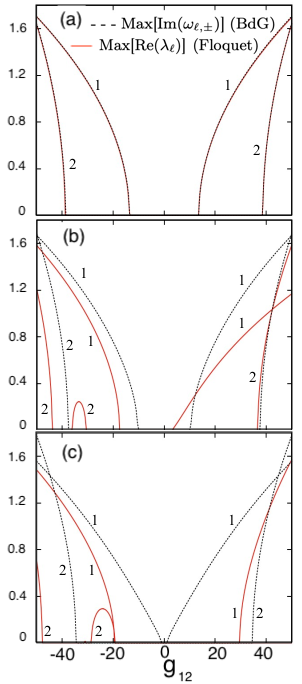
Figure 13: (Color online) Maximum unstable spectra for angular modes $\ell$ [$(=1,2)$, as indicated] are shown as functions of $g_{12}$, with fixed $g=1$ and frequencies $\Omega=$0.01, 0.50, and 0.99 [respectively, in panels (a), (b), and (c)]. With Max[Im($\omega_{\ell,\pm}$)] obtained from (23), the BdG unstable spectra are shown with black-dashed lines. Floquet unstable spectra, from (33), provided by Max[Re($\lambda_{\ell}$)], are with red-solid lines. Within defined units, all quantities are presented as dimensionless.

In Fig. 13, we set together all stability approximations previously discussed in order to observe more closely how the approaches are related to each other. In panels 13 (a), 13 (b) and 13 (c) we display three different regimes of Rabi coupling. In the weak regime $\Omega=0.01$, we see both, BdG and Floquet, approaches return about the same spectrum as already expected. Conversely, when the Rabi coupling constant is increased, the spectrum of the analytical approaches becomes quite different from each other.

A deeper analysis is provided in Fig. 14, which displays simultaneously the different roles of the Rabi coupling depending on the inter-species interaction. It is very clear that the coupling is able to open a large region of stability, which makes the unstable behavior to be postponed. But in some situations, it can make the system unstable, even when the BdG spectrum provides no trace of instability.

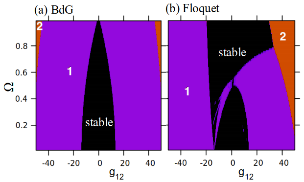
Figure 14: (Color online) Stability diagrams of Rabi parameter $\Omega$ versus $g_{12}$ for fixed $g=1$, given by Max[Im($\omega_{\ell,\pm}$)], representing stable regions ($\leq 0$, Black regions), and unstable ones [Violet, for $\ell=1$ and orange, for $\ell=2$]. BdG approach is in (a) [see (23)], with Floquet approach in (b) [see (35)]. Within defined units, all quantities are presented as dimensionless.

This phenomenon is also depicted for fixed parameters in Fig. 15. We display the two different sets of interaction parameters ($g$, $g_{12}$) $=$ (1, 15) and (40, -10), the first one is driven from an unstable to a stable solution by the increasing of the Rabi coupling, and the second one is led from a stable regime to an unstable one when the coupling becomes higher.

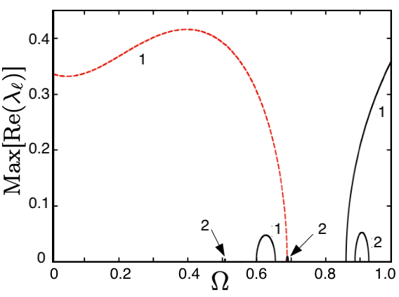
Figure 15: (Color online) Floquet maximum spectra (Max[Re($\lambda_{\ell}$)]) of unstable angular modes $\ell=1,2$ (indicated by the numbers) as functions of the coupling $\Omega$ [see (33)]. Cases ($g$, $g_{12}$) $=$ (1, 15) and (40, -10) are displayed with red-dashed and black-solid lines, respectively. Within defined units, all quantities are presented as dimensionless.

Table 1: Dynamics stability status of the BEC mixture by the three methods, given the parameter of intra- and inter-species interaction, and Rabi coupling constant $\Omega$, $g$, and $g_{12}$, respectively. Unstable cases are displayed with the dominant unstable mode $\ell$. The reference figures where the results can be checked are set in parentheses.

$\Omega$	$g$	$g_{12}$	BdG	Floquet	Dynamics
0.50	1	8	stable	$\ell=1$	$\ell=1$
			(13b)	(13b)	(7, 8a, 10)
0.94	40	-10	stable	$\ell=1$	$\ell=1$
			(3b )	(15)	(7, 8b, 9a, 11a-c)
0.10	1	10	stable	stable	stable
			(3a)	(4a)	(7)
0.99	1	25	$\ell=1$	stable	stable
			(13c)	(13c)	(7)
0.90	-10	20	$\ell=1$	$\ell=2$	$\ell=2$
			(3b)	(4b)	(9b, 11e-f)

In table 1, we compare the predictions of BdG and Floquet methods with the full dynamics calculations for the five sets of parameters ($\Omega$, $g$, $g_{12}$) mostly discussed in the text. We can check that the Floquet spectrum agrees with the dynamics simulations for all cases, then it is more suitable for our system than the BdG method.

Appendix D Resonance conditions

In the regime $g_{12}\ll g$ (or, equivalently, $\Delta g\ll g$ ), let us consider $\psi_{j}(\theta,\phi,t)=\phi_{j}(t){\mathrm{e}}^{-{\mathrm{i}}(\mu+\delta\mu)t},$ where $\mu=(2g+\Delta g)/(8\pi)$ is the chemical potential, with a $\Delta g$- first- order phase correction $\delta\mu=-\Delta g/(16\pi)$. The functions $\phi_{j}(t)$ given by $\phi_{1}=({1}/{\sqrt{4\pi}}\cos\left(\Omega t+\frac{\pi}{4}\right)\left[1+{\rm i}\Delta(t)\right]$, $\phi_{2}=({1}/{\sqrt{4\pi}}\sin\left(\Omega t+\frac{\pi}{4}\right)\left[1-{\rm i}\Delta(t)\right]$ where we are taking into account a time-dependent $\Delta g$- first-order correction function of interaction difference $\Delta g$, given by $\Delta(t)=\frac{\Delta g}{32\pi\Omega}\cos(2\Omega t)$. Small amplitude fluctuations around $\psi_{j}(\theta,\phi,t)$ are assumed, as

$$\psi_{j}(\theta,\phi,t) = [\phi_{j}(t)+\delta\phi_{j}(\theta,\phi,t)].$$ (61)

Now, we apply the following useful transformation from $(\delta\phi_{1},\delta\phi_{2})$ to $(\delta\phi_{d},\delta\phi_{s})$ 2022Zhang , in which terms higher than first order $\Delta(t)$ are neglected:

$$\begin{pmatrix}\delta\phi_{d}\\ \delta\phi_{s}\end{pmatrix} = \begin{pmatrix}{\phi}_{1}^{*}&&{\phi}_{2}^{*}\\ -{\phi}_{2}&&{\phi}_{1}\end{pmatrix}\begin{pmatrix}\delta\phi_{1}\\ \delta\phi_{2}\end{pmatrix},$$ (62a)

$$\begin{pmatrix}\delta\phi_{1}\\ \delta\phi_{2}\end{pmatrix} = 4\pi\begin{pmatrix}\phi_{1}&&-{\phi}_{2}^{*}\\ {\phi}_{2}&&{\phi}_{1}^{*}\end{pmatrix}\begin{pmatrix}\delta\phi_{d}\\ \delta\phi_{s}\end{pmatrix}.$$ (62b)

With (61) and the above inserted in (1) (neglecting 2nd and higher-order terms in $\Delta g$, $\delta\phi_{d}$, and $\delta\phi_{s}$), the following coupled equation for the excitations is obtained:

$${\mathrm{i}}\frac{\partial\delta\phi_{d}}{\partial t} = \Big{\{}-\frac{1}{2}\nabla^{2}+\frac{g}{4\pi}+\frac{\Delta g}{16\pi}\left[1+2\cos(4\Omega t)\right]\Big{\}}\delta\phi_{d}$$ (63)

$$+ \Big{\{}\frac{g}{4\pi}+\frac{\Delta g}{16\pi}\left[1+\cos(4\Omega t)\right]\Big{\}}\delta{\phi}_{d}^{*}$$

$$+ \Big{\{}\frac{\Delta g-2g}{8\pi}\delta{\phi}_{s}-\frac{\Delta g+3g}{16\pi}\delta{\phi}_{s}^{*}\Big{\}}\sin(4\Omega t),$$

$${\mathrm{i}}\frac{\partial\delta\phi_{s}}{\partial t} = \Big{\{}-\frac{1}{2}\nabla^{2}+\frac{\Delta g}{16\pi}\left[1-2\cos(4\Omega t)\right]\Big{\}}\delta\phi_{s}$$ (64)

$$- \Big{\{}\frac{\Delta g}{16\pi}\left[1+\cos(4\Omega t)\right]\Big{\}}\delta{\phi}_{s}^{*}$$

$$- \Big{\{}\frac{\Delta g}{8\pi}\delta{\phi}_{d}+\frac{\Delta g}{16\pi}\delta{\phi}_{d}^{*}\Big{\}}\sin(4\Omega t),$$

leading to a BdG matrix determinant for the spectrum, $|{\bf Z}-\omega_{\ell}|=0$, where, in 1st-order of $\Delta g$ and dropping the sinusoidal terms 2019Chen (nullified in the respective periods)

$${\bf Z}=\begin{pmatrix}\epsilon_{\ell}+\frac{4g+\Delta g}{16\pi}&\frac{4g+\Delta g}{16\pi}&0&0\\ -\frac{4g+\Delta g}{16\pi}&-\epsilon_{\ell}-\frac{4g+\Delta g}{16\pi}&0&0\\ 0&0&\epsilon_{\ell}+\frac{\Delta g}{16\pi}&-\frac{\Delta g}{16\pi}\\ 0&0&\frac{\Delta g}{16\pi}&-\epsilon_{\ell}-\frac{\Delta g}{16\pi}\end{pmatrix}.$$ (65)

The solution leads to the natural elementary excitations:

$$\omega_{d}^{2}={\epsilon_{\ell}\left(\epsilon_{\ell}+\frac{g}{2\pi}+\frac{\Delta g}{8\pi}\right)},\;{\rm and}\;\omega_{s}^{2}={\epsilon_{\ell}\left(\epsilon_{\ell}+\frac{\Delta g}{8\pi}\right)}.$$ (66)

References

- (1) M. C. Cross and P. C. Hohenberg, Pattern formation outside of equilibrium, Rev. Mod. Phys. 65, 851 (1993).
- (2) M. Faraday, XVII. On a peculiar class of acoustical figures; and on certain forms assumed by groups of particles upon vibrating elastic surfaces, Phil. Trans. R. Soc. London 121, 299 (1831).
- (3) M. H. Anderson, J.R. Ensher, M. R. Matthews, C.E. Wieman, and E. A. Cornell, Observation of Bose-Einstein condensation in a dilute atomic vapor, Science 269, 198 (1995).
- (4) K. B. Davis, M. -O. Mewes, M. R. Andrews, N.J. van Druten, D. S. Durfee, D. M. Kurn, and W. Ketterle, Bose-Einstein condensation in a gas of sodium atoms, Phys. Rev. Lett. 75, 3969 (1995).
- (5) C. C. Bradley, C. A. Sackett, J. J. Tollett, and R. G. Hulet, Evidence of Bose-Einstein condensation in an atomic gas with attractive interactions, Phys. Rev. Lett. 75, 1687 (1995).
- (6) F. Dalfovo, S. Giorgini, L. P. Pitaevskii, and S. Stringari, Theory of Bose-Einstein condensation in trapped gases, Rev. Mod. Phys. 71, 463 (1999).
- (7) L. Pitaevskii and S. Stringari, Bose-Einstein condensation and superfluidity, Oxford Sci. Publ. (2016).
- (8) K. Staliunas, S. Longhi, and G. J. de Valcárcel, Faraday patterns in Bose-Einstein condensates, Phys. Rev. Lett. 89, 210406 (2002).
- (9) P. Engels, C. Atherton, and M. A. Hoefer, Observation of Faraday waves in a Bose-Einstein condensate, Phys. Rev. Lett. 98, 095301 (2007).
- (10) R. Nath and L. Santos, Faraday patterns in two-dimensional dipolar Bose-Einstein condensates, Phys. Rev. A 81, 033626 (2010).
- (11) J. B. Sudharsan, R. Radha, M. C. Raportaru, A. I. Nicolin, and A. Balaž, Faraday and resonant waves in binary collisionally-inhomogeneous Bose–Einstein condensates, J. Phys. B: At. Mol. Opt. Phys. 49, 165303 (2016).
- (12) F. Kh. Abdullaev, A. Gammal, and L. Tomio, Faraday waves in Bose-Einstein condensates with engineering three-body interactions, J. Phys. B: At. Mol. Opt. Phys. 49, 025302 (2016).
- (13) F. Kh. Abdullaev, A. Gammal, R. K. Kumar, and L. Tomio, Faraday waves and droplets in quasi-one- dimensional Bose gas mixtures, J. Phys. B: At. Mol. Opt. Phys. 52, 195301 (2019).
- (14) J. Smits, L. Liao, H. T. C. Stoof, and P. van der Straten, Observation of a space-time crystal in a superfluid quantum gas, Phys. Rev. Lett. 121, 185301 (2018).
- (15) J. H. V. Nguyen, M. C. Tsatsos, D. Luo, A. U. J. Lode, G. D. Telles, V. S. Bagnato, and R. G. Hulet, Parametric excitation of a Bose-Einstein condensate: From Faraday waves to granulation, Phys. Rev. X 9, 011052 (2019)
- (16) Z. Zhang, K.-X. Yao, L. Feng, J. Hu, and C. Chin, Pattern formation in a driven Bose-Einstein condensate, Nature Physics 16, 652 (2020).
- (17) D. K. Maity, K. Mukherjee, S. I. Mistakidis, S. Das, P. G. Kevrekidis, S. Majumder, and P. Schmelcher, Parametrically excited star-shaped patterns at the interface of binary Bose-Einstein condensates, Phys. Rev. A 102, 033320 (2020).
- (18) K. Kwon, K. Mukherjee, S. J. Huh, K. Kim, S. I. Mistakidis, D. K. Maity, P. G. Kevrekidis, S. Majumder, P. Schmelcher, and J.-y. Choi, Spontaneous Formation of Star-Shaped Surface Patterns in a Driven Bose-Einstein Condensate, Phys. Rev. Lett. 127, 113001 (2021).
- (19) K. Fujii, S. L. Görlitz, N. Liebster, M. Sparn, E. Kath, H. Strobel, M. K. Oberthaler, and T. Enss, Square pattern formation as stable fixed point in driven two-dimensional Bose-Einstein condensates, arXiv:2309.03829v2 [cond-mat.quant-gas].
- (20) R. Cominotti, A. Berti, A. Farolfi, A. Zenesini, G. Lamporesi , I. Carusotto , A. Recati, and G. Ferrari, Observation of massless and massive collective excitations with Faraday patterns in a two-component superfluid, Phys. Rev. Lett. 128, 210401 (2022).
- (21) E. Timmermans, P. Tommasini, M. Hussein, A. Kerman, Feshbach resonances in atomic Bose–Einstein condensates, Phys. Rep. 315, 199 (1999).
- (22) L. B. da Silva, and E. F. de Lima, Coherent control of nonlinear mode transitions in Bose-Einstein condensates, J. Phys. B: At. Mol. Opt. Phys. 53, 125302 (2020).
- (23) C.-X. Zhu, W. Yi, G.-C. Guo, and Z.-W. Zhou, Parametric resonance of a Bose-Einstein condensate in a ring trap with periodically driven interactions, Phys. Rev. A 99, 023619 (2019).
- (24) M. Grifoni and P. Hänggi, Driven quantum tunneling,Physics Reports 304, 229 (1998).
- (25) J. Williams, R. Walser, J. Cooper, E. A. Cornell, and M. Holland, Excitation of a dipole topological state in a strongly coupled two-component Bose-Einstein condensate, Phys. Rev. A 61, 033612 (2000).
- (26) Y. He, H. Guo, and C.-C. Chien, BCS-BEC crossover of atomic Fermi superfluid in a spherical bubble trap, Phys. Rev. A 105, 033324 (2022).
- (27) L. Amico, D. Anderson, M. Boshier, J.-P. Brantut, L.-C. Kwek, A. Minguzzi, and W. von Klitzing, Colloquium: Atomtronic circuits: From many-body physics to quantum technologies, Rev. Mod. Phys. 94, 041001 (2022).
- (28) B. Kh. Tumanov, B. B. Baizakov, F. Kh. Abdullaev, Generation of density waves in dipolar quantum gases by time-periodic modulation of atomic interactions, Phys. Rev. A 101, 053616 (2020).
- (29) T. Chen, K. Shibata, Y. Eto, T. Hirano, and H. Saito, Faraday patterns generated by Rabi oscillation in a binary Bose-Einstein condensate, Phys. Rev. A 100, 063610 (2019).
- (30) S. D. Jenkins and T. A. B. Kennedy, Dynamic stability of dressed condensate mixtures, Phys. Rev. A 68, 053607 (2003).
- (31) K. Shibata, A. Torii, H. Shibayama, Y. Eto, H. Saito, and T. Hirano, Interaction modulation in a long-lived Bose-Einstein condensate by rf coupling, Phys. Rev. A 99, 013622 (2019).
- (32) L. D. Landau and E. M. Lifshitz, Mechanics, Pergamon, Oxford, (1960).
- (33) H. Zhang, S. Liu, and Y. Zhang, Faraday patterns in spin-orbit-coupled Bose-Einstein condensates, Phys. Rev. A 105, 063319 (2022).
- (34) C. J. Myatt, E. A. Burt, R. W. Ghrist, E. A. Cornell, and C. E. Wieman, Production of two overlapping Bose-Einstein condensates by sympathetic cooling, Phys. Rev. Lett. 78, 586 (1997).
- (35) G. Modugno, M. Modugno, F. Riboli, G. Roati, and M. Inguscio, Two atomic species superfluid, Phys. Rev. Lett. 89, 190404 (2002).
- (36) O. E. Alon, Fragmentation of identical and distinguishable bosons’ pairs and natural geminals of a trapped bosonic Mixture, Atoms 9, 92 (2021).
- (37) M. Brtka, A. Gammal, and B. A. Malomed, Hidden vorticity in binary Bose-Einstein condensates, Phys. Rev. A 82, 053610 (2010).
- (38) A. Andriati, L. Brito, L. Tomio, and A. Gammal, Stability of a Bose-condensed mixture on a bubble trap, Phys. Rev. A 104, 033318 (2021).
- (39) O. Zobay and B. M. Garraway, Two-dimensional atom trapping in field-induced adiabatic potentials, Phys. Rev. Lett. 86, 1195 (2001).
- (40) O. Zobay and B. M. Garraway, Atom trapping and two-dimensional Bose-Einstein condensates in field-induced adiabatic potentials, Phys. Rev. A 69, 023605 (2004).
- (41) D. C. Aveline, J. R. Williams, E. R. Elliott, C. Dutenhoffer, J. R. Kellogg, J. M. Kohel, N. E. Lay, K. Oudrhiri, R. F. Shotwell, N. Yu, and R. J. Thompson, Observation of Bose–Einstein condensates in an Earth-orbiting research lab, Nature 582, 193 (2020).
- (42) R. A. Carollo, D. C. Aveline, B. Rhyno, S. Vishveshwara, C. Lannert, J. D. Murphree, E. R. Elliott, J. R. Williams, R. J. Thompson, and N. Lundblad, Observation of ultracold atomic bubbles in orbital microgravity, Nature 606, 281 (2022).
- (43) N. Lundblad, D. C. Aveline, A. Balaž, E. Bentine, N. P. Bigelow, P. Boegel, M. A. Efremov, N. Gaaloul, M. Meister, M. Olshanii, C. A. R. Sá de Melo, A. Tononi, S. Vishveshwara, A. C. White, A. Wolf, and B. M. Garraway, Perspective on quantum bubbles in microgravity, Quantum Sci. Technol. 8, 024003 (2023).
- (44) F. Jia, Z. Huang, L. Qiu, R. Zhou, Y. Yan, and D. Wang, Expansion dynamics of a shell-shaped Bose-Einstein condensate, Phys. Rev. Lett. 129, 243402 (2022).
- (45) Y. Guo, E. M. Gutierrez, D. Rey, T. Badr, A. Perrin, L. Longchambon, V. S. Bagnato, H. Perrin and R. Dubessy, Expansion of a quantum gas in a shell trap, New J. Phys. 24, 093040 (2022).
- (46) A. Tononi and L. Salasnich, Low-dimensional quantum gases in curved geometries, Nat. Rev. Phys. 5, 398 (2023).
- (47) K. Padavić, K. Sun, C. Lannert, and S. Vishveshwara, Physics of hollow Bose-Einstein condensates, Europhys. Lett. 120, 20004 (2018).
- (48) K. Sun, K. Padavić, F. Yang, S. Vishveshwara, and C. Lannert, Static and dynamic properties of shell-shaped condensates, Phys. Rev. A 98, 013609 (2018).
- (49) S. J. Bereta, L. Madeira, V. S. Bagnato, and M. A. Caracanhas, Bose-Einstein condensation in spherically symmetric traps, Am. J. Phys. 87, 924 (2019).
- (50) A. Tononi and L. Salasnich, Bose-Einstein condensation on the surface of a sphere, Phys. Rev. Lett. 123, 160403 (2019).
- (51) N. S. Móller, F. E. A. dos Santos, V.S. Bagnato, and A. Pelster, Bose–Einstein condensation on curved manifolds, New J. Phys. 22, 063059 (2020).
- (52) K. Padavić, K. Sun, C. Lannert, and S. Vishveshwara, Vortex-antivortex physics in shell-shaped Bose-Einstein condensates, Phys. Rev. A 102, 043306 (2020).
- (53) M. A. Caracanhas, P. Massignan, and A. L. Fetter, Superfluid vortex dynamics on an ellipsoid and other surfaces of revolution, Phys. Rev. A 105, 023307 (2022).
- (54) H. Saito and M. Hayashi, Rossby–Haurwitz wave in a rotating bubble-shaped Bose–Einstein condensate, J. Phys. Soc. Jpn. 92, 044003 (2023).
- (55) S. K. Adhikari. Dipolar Bose-Einstein condensate in a ring or in a shell, Phys. Rev. A 85, 053631 (2012).
- (56) P. C. Diniz, E. A. B. Oliveira, A. R. P. Lima, and E. A. L. Henn, Ground state and collective excitations of a dipolar Bose-Einstein condensate in a bubble trap, Sci. Rep. 10, 4831 (2020).
- (57) A. Tononi, A. Pelster, and L. Salasnich, Topological superfluid transition in bubble-trapped condensates, Phys. Rev. Res. 4, 013122 (2022).
- (58) S. Prestipino and P. V. Giaquinta, Ground state of weakly repulsive soft-core bosons on a sphere, Phys. Rev. A 99, 063619 (2019).
- (59) B. Rhyno, N. Lundblad, D. C. Aveline, C. Lannert, and S. Vishveshwara, Thermodynamics in expanding shell-shaped Bose-Einstein condensates, Phys. Rev. A 104, 063310 (2021).
- (60) P. Stürmer, M. N. Tengstrand, and S. M. Reimann, Mixed bubbles in a one-dimensional Bose-Bose mixture, Phys. Rev. Res. 4, 043182 (2022).
- (61) A. H. Salas, J. E. Castillo H., Exact solution to Duffing equation and the pendulum equation, Appl. Math. Sci. 8, 8781 (2014).
- (62) A. Beléndez, T. Beléndez, F. J. Martínez, C. Pascual, M. L. Alvarez, and E. Arribas, Exact solution for the unforced Duffing oscillator with cubic and quintic nonlinearities, Nonlinear Dyn. 86, 1687 (2016).
- (63) E. T. Whittaker and G. N. Watson, A course of modern analysis, Cambridge University Press, Cambridge, 5th ed., 2021, edited and prepared by V. H. Moll.
- (64) V. M. Kenkre and G. P. Tsironis, Nonlinear effects in quasielastic neutron scattering: Exact line-shape calculation for a dimer, Phys. Rev. B 35, 1473 (1987).