GALAXY CRUISE: Deep Insights into Interacting Galaxies in the Local Universe

Abstract

We present the first results from GALAXY CRUISE, a community (or citizen) science project based on data from the Hyper Suprime-Cam Subaru Strategic Program (HSC-SSP). The current paradigm of galaxy evolution suggests that galaxies grow hierarchically via mergers, but our observational understanding of the role of mergers is still limited. The data from HSC-SSP are ideally suited to improve our understanding with improved identifications of interacting galaxies thanks to the superb depth and image quality of HSC-SSP. We have launched a community science project, GALAXY CRUISE, in 2019 and collected over 2 million independent classifications of 20,686 galaxies at $z<0.2$. We first characterize the accuracy of the participants’ classifications and demonstrate that it surpasses previous studies based on shallower imaging data. We then investigate various aspects of interacting galaxies in detail. We show that there is a clear sign of enhanced activities of super massive black holes and star formation in interacting galaxies compared to those in isolated galaxies. The enhancement seems particularly strong for galaxies undergoing violent merger. We also show that the mass growth rate inferred from our results is roughly consistent with the observed evolution of the stellar mass function. The 2nd season of GALAXY CRUISE is currently under way and we conclude with future prospects. We make the morphological classification catalog used in this paper publicly available at the GALAXY CRUISE website, which will be particularly useful for machine-learning applications.

1 Introduction

Astronomy is one of the research fields where not only professional researchers but the general public as well have made significant contributions to advance the field. An old example can be found back in the 18th century when Edmond Halley asked ‘the Curious’ to observe the total solar eclipse over England (Pasachoff, 1999). Astronomy has a long tradition of active contributions of the general public and amateur astronomers, and new discoveries of interesting objects such as comets and supernovae are often reported even today, some of which are followed up by professional astronomers with a larger telescope for detailed studies. This teamwork between non-professional and professional researchers has been extremely fruitful to improve our understanding of the Universe.

A new area of such collaboration emerged with the advent of large sky surveys, which observe billions of celestial objects in a large area of the sky. While objects from these surveys are detected and measured in an automated fashion, not all properties of the objects can be fully captured and cataloged. Galaxy morphology is one such property; there is no easy measurement that fully describes the entire variation of galaxy morphology. Morphology has traditionally been classified by human eyes as they are good at recognizing characteristic patterns in an image such as spiral arms. A number of automated methods have been proposed such as concentration index (Morgan, 1958; Doi et al., 1993; Abraham et al., 1994), Sersic index (Sersic, 1968), Gini coefficient (Abraham et al., 2003), etc, but human classifications still remain highly complementary to these automated classifications.

Galaxy Zoo (Lintott et al., 2008) is the first large-scale citizen science (hereafter community science) project based on the imaging data from the Sloan Digital Sky Survey (SDSS; York et al. (2000)). Participants classify morphologies of objects in the SDSS image and a large number of independent classifications have been collected for nearly a million objects. There are many scientific papers based on the Galaxy Zoo’s classifications published to date. Galaxy Zoo is undoubtedly the most successful community science project in astronomy and the successor and spin-off projects such as Galaxy Zoo 2 (Willett et al., 2013) have also been successful.

The Galaxy Zoo’s classifications (Lintott et al., 2008) are fundamentally limited by the imaging quality of SDSS. While SDSS delivered the state of the art imaging data at that time, recent imaging surveys such as Dark Energy Survey (DES; The Dark Energy Survey Collaboration (2005)), PanSTARRS1 (PS1; Chambers et al. (2016)), and Hyper Suprime-Cam Subaru Strategic Program (HSC-SSP; Aihara et al. (2018b)) yield deeper images, which help improve the classification accuracy. Among these surveys, HSC-SSP is particularly interesting due to its superb image quality and depth; the median seeing in the $i$-band is 0.6 arcsec and the images reach 26-27th magnitude, i.e., 2-4 magnitudes deeper than SDSS, DES and PS1. The depth is particularly important to detect faint spirals arms as well as diffuse tidal features as we demonstrate in this paper.

Based on the imaging data from HSC-SSP, we have launched GALAXY CRUISE, the first Japanese community science project in astronomy. In order to fully exploit the superb imaging data, we put an emphasis on interacting galaxies. In the bottom-up galaxy formation scenario, we expect that galaxy-galaxy mergers play a fundamental role in the evolution of galaxies over the cosmic time. However, our understanding of mergers is is still limited; frequency of mergers, triggering of starburst and active galactic nuclei (AGN) still remain unclear. This is largely due to the difficulty of identifying interacting/merging galaxies. A traditional way to identify mergers is to look for tidal features around galaxies, but these features are typically very faint and deep imaging data is essential to identify them (e.g., Lotz et al. (2008); Tal et al. (2009); Duc et al. (2015); Bottrell et al. (2019); Wilkinson et al. (2022)). To avoid this difficulty, close pairs are also often used to estimate the merger rate (Patton et al., 2000, 2002; Lin et al., 2004). But, close pairs have their own difficulties such as contamination of line-of-sight pairs that are not physically bound and a lack of sensitivity to post-merger phases. We focus on the former approach to fully exploit the imaging depth of HSC-SSP in this paper and present the first results from GALAXY CRUISE.

The paper is organized as follows. We introduce GALAXY CRUISE and discuss classification statistics in Section 2. We then characterize the classification accuracy in Section 3. Based on the participants’ classifications, we make comparisons to previous community science projects and also examine properties of interacting galaxies in Section 4. Finally, the paper is summarized in Section 5. Unless otherwise stated, we use the AB magnitude system (Oke & Gunn, 1983) and the adopt the flat cosmology with $\rm H_{0}=70\ km\ s^{-1}\ Mpc^{-1}$, $\rm\Omega_{M}=0.3$, and $\Omega_{\Lambda}=0.7$.

2 GALAXY CRUISE

2.1 Motivation

We focus on interacting galaxies to address some of the outstanding questions about galaxy mergers as discussed in the previous Section. As interacting galaxies are a rare population, we need to inspect many galaxies to gain sufficient statistics to study their properties. However, the visual inspection of tens of thousands of galaxies is difficult to perform by professional astronomers as astronomers are a rare population. This is where the interested general public can significantly contribute as Galaxy Zoo demonstrated. We follow the same approach and ask participants to classify galaxies and find interacting galaxies.

A community science project is not just a science project, but it also has a major aspect of public engagement. We put an emphasis on this aspect in GALAXY CRUISE and implemented a lot of gamification factors to motivate and entertain participants as they classify objects. As part of this, we made the theme of the classification site a cruise ship sailing across the cosmic ocean, hence the name GALAXY CRUISE. Participants collect passport stamps and souvenirs as they make progress. There are also seasonal campaigns to make, e.g., a snowman as they classify. We encourage participants not just classify targets but also freely explore the vast Universe. For this, we do not to show postage stamps of galaxies and instead show the entire sky observed by HSC-SSP as a contiguous image. The contiguous image is essential also for identifications of tidal features; we do not know a priori where tidal features are and some of them may be located far away from the central galaxy. A fixed-scale postage-stamp may miss such features, but the contiguous image does not. A screenshot of our classification site is shown in Fig. 1.

As mentioned above, we use publicly available images from HSC-SSP. HSC-SSP is a wide and deep survey of the sky using HSC installed at the Subaru Telescope. It has three survey layers. The Wide survey covers $\sim 1,100$ square degrees of the sky located mostly around the equator in five broad-band filters ($grizy$) down to $r\sim 26.5$ for point sources at $5\sigma$. The Deep survey has four fields separated roughly equally in R.A., so that one of them is observable at any time. The Deep survey typically goes a magnitude deeper than Wide. Finally, the UltraDeep survey is 2 fields, COSMOS and SXDS, reaching down to $\sim 28$th mag. Further details of the survey can be found in Aihara et al. (2018a). The HSC-SSP data are routinely made public and we use mulit-band images from HSC-SSP Public Data Relase 2 (PDR2; Aihara et al. (2019)), which was the latest release when our project started. Most of our targets are from the Wide survey, but we also include objects from the Deep and UltraDeep surveys allowing for duplication, so that we can characterize the dependence on the depth in our classifications (see the next Section for details). Table 2 of Aihara et al. (2019) summarizes the quality of the imaging data. We combine the $g$, $r$, and $i$-bands to generate color images of the sky using Lupton et al. (2004) scheme. Participants can adjust levels so that bright/faint parts of targets can be easily seen. This feature is particularly useful for identifying interaction features, which are often diffuse and extended. Also, single-filter black/white images are available for detailed inspections.

While our primary objective is to identify interacting galaxies, we are also interested in the morphology of normal (non-interacting) galaxies because the depth and quality of HSC may bring a difference in our basic understanding of galaxy morphology in the local Universe. We choose to make two-step classifications; first is to classify morphology of galaxies such as elliptical and spiral, and the second is to look for interaction features. There are multiple morphology classification schemes. Some are rather complicated and difficult, while others are more straightforward. How detailed classification participants can make with what accuracy is not a trivial question to answer.

In order to address the question, we made public experiments at National Museum of Emerging Science and Innovation (Miraikan) in Tokyo. We display a large-format poster of a contiguous region of the sky taken by HSC-SSP. We made an introductory lecture about galaxy morphology to participants and asked them to classify target galaxies marked on the poster. We also directly talked to them to see how they recognize various features of galaxies.

Lessons learned from the experiment include: (1) the general public can classify bright galaxies reasonably well, but (2) faint galaxies (for which basic classifications can still be made by professional astronomers) are very difficult, and (3) subtle differences such as presence of weak bars, elliptical vs S0, etc are difficult to recognize. Following these lessons, we choose to focus on bright galaxies and adopt a simple classification scheme, which we detail in the next subsection. Another lesson learned from the experiment is that edge-on spirals tend to be classified as ellipticals. While we made an attempt to make the difference clear in the tutorial, this tendency is still observed in our classifications in GALAXY CRUISE. The introductory lecture used in the experiment turned into training courses for first-time participants at the GALAXY CRUISE website. Overall, the public experiment was an essential piece of our project.

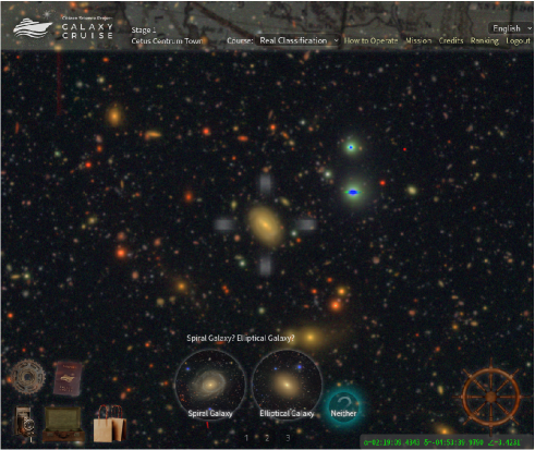
Figure 1: GALAXY CRUISE’s classification screen. Participants classify the target at the center, and then ’sail’ to the next target. Passport stamps, souvenirs and other features are available to motivate the participants.

2.2 Classification Scheme

Fig. 2 shows our classification flow. The first question is whether a galaxy is an elliptical galaxy or spiral galaxy. As described earlier, subtle differences between ellipticals and S0’s and bar structure are difficult to distinguish for the general public. We thus choose to adopt the simplified classification scheme. Some interacting galaxies show significantly distorted shapes and their original morphology can be difficult to infer. In such a case, the participant can choose ‘not sure’. When a target galaxy is too close to a nearby bright star and a fair classification is difficult, the participant can choose ‘not sure’ as well.

The 2nd question is whether there is a sign of interaction or not. Interacting galaxies exhibit a variety of features, but we define 4 typical features; (1) tidal tail/stream, (2) distorted shape, (3) fan/shell structure, and (4) ring structure. The first feature is perhaps the most prominent feature seen around interacting galaxies; leading/trailing streams are formed by stars escaping from an infalling galaxy mostly through the Lagrange points $L_{1}$ and $L_{2}$ due to tidal disruption (Eyre & Binney, 2011). A distorted shape is also a common feature and is also caused by tidal forces. A fan/shell feature is likely a special case of collision with a small impact parameter (i.e., low angular momentum), which results in two-sided caustics with large opening angles (Pop et al., 2018). Finally, the ring structure can be formed by multiple processes including secular process, but galaxy-galaxy interactions are a strong theory for the origin of ring galaxies (e.g., Elagali et al. (2018)) and we interpret the ring structure as a possible sign of interaction.

One can choose multiple interaction features for a given object. This is because multiple features are often seen (especially distortion and tail) and also because some of the features are not easily distinguishable (e.g., arc-like tail vs. fan). As we will discuss below, tail and distortion features are the most common features and ring and fan features are less often observed.

Before a participant joins GALAXY CRUISE and start to make classifications, we ask the participant to go over an online introductory course, which is based on the tutorial from the public experiment as mentioned above, to understand our classification scheme. The online course is a three-step tutorial. We first explain the primary differences between elliptical and spiral galaxies such as the presence of spiral arms and disk structure. We then show that galaxies are normally symmetric in shape and deviations from the symmetry is often an indication of interaction. Finally, we introduce the four typical interaction features discussed above. We ask several questions to the participant at each step to make sure the participant understands the scheme. These three steps are identical to the questions shown in Fig. 2. In other words, we explain each question in the tutorial. After the tutorial, the participant gets a ’boarding pass’ to join GALAXY CRUISE. For further details, the reader is referred to the GALAXY CRUISE website.

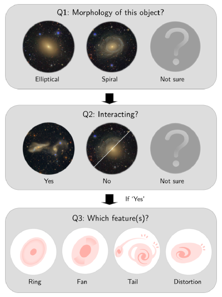
Figure 2: GALAXY CRUISE’s classification scheme. The first question is whether a galaxy is spiral or elliptical. The second question asks if the galaxy is interacting or not. If yes, the participant can choose observed feature(s).

2.3 Target Galaxies

GALAXY CRUISE is based on deep imaging data from HSC-SSP PDR2 (Aihara et al., 2019), in which the global sky subtraction was applied to keep extended wings of bright objects. This is an ideal feature for our purpose as interaction features are often diffuse and extended.

The target galaxies for classifications are drawn from spectroscopic data from the Sloan Digital Sky Survey (SDSS; York et al. (2000)) and the GAMA survey (Driver et al., 2009). The reasons why we draw targets from the spectrscopic data include (1) they are bright objects for which the participants can make good classifications (see Section 2.1), and (2) the distance information allows us to accurately infer physical properties of galaxies such as star formation rates (SFRs) from emission line fluxes, and (3) the spectra allow us to identify active galactic nuclei (AGN) from emission line intensity ratios. The SDSS main galaxy sample (Strauss et al., 2002) is primarily used here, but any objects with spectroscopic redshifts from Data Release 15 (Aguado et al., 2019) located at $z<0.2$ are included. We imposed this redshift cut to make sure we focus on nearby galaxies for which we expect to have sufficient spatial resolution to classify. We supplement the SDSS redshifts with those from GAMA DR2 (Liske et al., 2015) to achieve a higher sampling rate. The same redshift cut of $z<0.2$ is imposed here as well. We then apply a magnitude cut to the cModel photometry in the $z$-band ($z_{cmodel}<17.0$) to the entire sample to ensure that we focus on very bright galaxies.

The magnitude cut was applied using the HSC photometry, which later turned out not to be the best choice; due to the high spatial resolution of HSC, bright galaxies, especially face-on spiral galaxies, are occasionally deblended into multiple pieces (Bosch et al., 2018; Aihara et al., 2019). This resulted in reduced brightness of the central galaxy, and a fraction of bright galaxies were excluded from the target sample by the magnitude cut. The same problem occurred in SDSS as well but to a lesser extent. A comparison between HSC and SDSS photometry indicates that this effect is not significant for most sources, but about 10% of the sources have fainter HSC photometry by more than 1 mag. In order to mitigate the problem, GALAXY CRUISE 2nd season has been running since April 2022. The 2nd season is an extension of the 1st season, but we target fainter galaxies without any magnitude cut including those that should have been targeted in the 1st season. They are still bright galaxies with spectroscopic redshifts following the lesson learned from the public experiment described in Section 2.1. We note that the all photometry used in what follows is from SDSS.

The targets are drawn from SDSS (18,960 galaxies) and GAMA (1,726 galaxies). Among them, 20,116 galaxies are in the Wide layer, and 1,410 galaxies are in the D/UD layer. As three of the four HSC-SSP D/UD fields are embedded in the Wide fields, 840 galaxies are duplicated and classified twice; once at the D/UD depth and once at the Wide depth. We evaluate how classifications change depending on the image depth in Section 3.1.

2.4 Combined Classifications

In this paper, we base our analysis on the classifications collected during the 1st season between November 2019 and April 2022. Due to the way classifications were made, a small number of participants classified the same objects multiple times. We use only the last classification. Fig. 3 shows the number of classifications made for each object. The median of the distribution is 83, which is sufficient for statistical classifications of objects. We define a probability that an object is a spiral galaxy as

$$P(spiral)=\frac{N_{spiral}}{N_{total}},$$ (1)

where $N_{total}$ is the total number of classifications made for that object, and $N_{spiral}$ is the number of spiral classifications among them. If $P(spiral)=1$, everyone agrees that an object is a spiral galaxy. If $P(spiral)=0$ instead, then everyone agrees that it is an elliptical galaxy. Of course, there are other types of galaxies in the Universe such as S0 galaxies, but we adopt this simplified classification scheme as discussed in Section 2.2. Strictly speaking, $P(spiral)$ is not a probability but just a fraction of classifications. However, we will later discuss fraction of spiral galaxies among our sample. In order to reduce confusions about which fraction we are discussing, we refer to the fraction of spiral classifications by the participants as spiral probability or $P(spiral)$. In the same manner, we define $P(int.)$, which indicates the fraction of people who vote for interaction in the 2nd question.

We first merge all of the individual classifications and compute $P(spiral)$. While most participants carefully classify objects, there are a small number of people whose classifications are less accurate. To make a reliable morphological catalog, we make an attempt to exclude those less-accurate participants. To this aim, we focus on galaxies with obvious morphologies, i.e., galaxies for which the vast majority of people agree on their morphological types. To be specific, we select objects with $P(spiral)<0.05$ or $P(spiral)>0.95$. These are clearly either elliptical or spiral. Such objects comprise about 10% of the entire sample. We then compile a list of participants whose classifications fall in the minority (i.e., likely incorrect). We define a probability that a participant makes an inaccurate classification as

$$P(bad)=\frac{N(bad)}{N(obvious)},$$ (2)

where $N(obvious)$ is the number of objects with obvious morphology that a participant classified, and $N(bad)$ is a subset of $N(obvious)$ and is the number of classifications that the participant falls in the minority. Fig. 4 shows $P(bad)$ against the total number of classification that a participant made. As can be seen, most participants make good classifications with low $P(bad)$, but there are people whose classifications are less accurate. We choose to exclude classifications by participants with $P(bad)>0.1$ in this work. This excludes 276,530 classifications out of total 2,431,455 classifications (11 %). We have confirmed that our results do not change if we include them. We note that Galaxy Zoo adopted a similar approach; they down-weighted participants who consistently disagreed with the majority. Note as well that there is a group of participants at $N_{\rm classification}\sim 1,000$ in Fig. 4. It is likely due to classification campaigns we have promoted, during which 1,000 classifications give participants a special image.

The hatched histogram in Fig. 3 shows the number of classifications for each object after the less accurate participants are excluded. The median number of classification is reduced from 83 to 74, but it is still sufficient for statistical analyses in this paper. We use $P(spiral)$ and $P(int.)$ after excluding these inaccurate classifiers in what follows.

For the first and second questions, we include the ’not sure’ option as shown in Fig. 2. This is intended to flag objects that are difficult to classify because the target is very strongly disturbed. We find that the majority (92%) of objects have $P(not\_sure)<0.1$ for the first question. Careful inspections of individual cases suggest that most participants did not choose ’not sure’ even when the target is strongly disturbed. For instance, objects with $P(not\_sure)\sim 0.3$ are often undergoing violent interactions, but $\sim 70\%$ of the participants classified them into elliptical/spiral. Also, it seems a small fraction of people used the ’not sure’ option for simply difficult cases (e.g., galaxies that appear small and hard to classify into ellitical or spiral). This was not our original intention for this option. The trend is similar for the second question; many of the objects with $P(not\_sure)>0.1$ are simply difficult cases such as targets in dense clusters, where the inracluster light is clearly visible.

As some fraction of participants used the ’not sure’ option in the way that we originally did not intend, we choose to exclude ’not sure’ votes when we compute $P(spiral)$ and $P(int.)$ (i.e., $N_{total}$ in Eq. 1 is equal to $N_{spiral}+N_{elliptical}$) because it is the least harmful way to handle them. We have confirmed that our conclusions remain the same if we include them (i.e., $N_{total}=N_{spiral}+N_{elliptical}+N_{not\_sure}$). We should emphasize, however, that the ’not sure’ votes are not useless; they actually turn out to be quite useful to identify violent mergers as we demonstrate below.

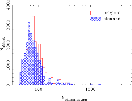
Figure 3: Distribution of the number of classifications for each object. The open histogram is the original classifications, while the shaded one is after the cleaning of bad classifications (see text for details). The median of the distribution is 83 for the original and 74 for the cleaned catalogs, respectively.

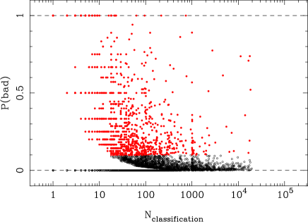
Figure 4: $P(bad)$ plotted against the total number of classification for each participant. Participants with $P(bad)>0.1$ (the red points) are excluded from the main analyses. The other participants shown in black are included.

3 Classification Accuracy

Visual classifications of galaxy morphology is dependent on the imaging depth, e.g., faint arms of a spiral galaxy may not be clearly identified in a shallow image. Diffuse tidal streams may be missed for the same reason. There is also redshift dependence as a faint feature is harder to identify at higher redshift. Furthermore, there may be yet another effect arising from systematic biases in the participants’ classifications. We make a few tests in this Section to characterize the depth and redshift dependence as well as classification biases.

3.1 Depth Dependence

We first focus on the dependence on the imaging depth. As we noted above, a small number of the targets are classified in both of the Wide and D/UD layers. This is done exactly for the purpose of the depth dependence characterization; as the D/UD layer is deeper than Wide layer (the typical exposure time is about 5 times longer; Aihara et al. (2019)), we can make a direct comparison between them for the same set of objects.

Fig. 5 makes this comparison and illustrates the role of depth at fixed resolution by comparing the Wide layer with the D/UD layer. $P(spiral)$ in the left panel shows that, while there is a good agreement at $P(spiral)\sim 0$ and 1, the different depths give a slightly different $P(spiral)$ at intermediate $P(spiral)$. We interpret this trend as spiral galaxies being more robustly identified in the deeper images. As we demonstrate below, GALAXY CRUISE finds a higher fraction of spiral galaxies compared to previous projects because of the much improved depth and quality. That is, spiral features can be more securely identified in deeper and sharper images. This explains the trend seen in Fig. 5; $P(spiral)$ tends to be larger in D/UD than in Wide for ambiguous cases. The depth difference is less important when a target galaxy is obviously elliptical or spiral, and $P(spiral)$ agrees well at 0 and 1.

The right panel, which shows $P(int.)$ for D/UD and Wide, can be explained in the same way. As interaction features are often faint and diffuse, deeper images reveal a larger fraction of interacting galaxies. The green points in both panels show the running median of the distribution and we use this curve to statistically correct $P(spiral)$ and $P(int.)$ from Wide to the D/UD depth. The correction would be larger if we had deeper images than D/UD (i.e., we would identify more interacting features if we could go deeper), but the green points in the figure are the correction we can make with the data in hand. We adopt the D/UD classifications whenever available (i.e., we exclude the Wide classifications for the duplicated objects), and apply the correction as shown by the green dots to objects classified only at the Wide depth to increase their $P(spiral)$ and $P(int.)$ to the D/UD depth. This leaves us 20,686 unique objects.

It is interesting to note that the $P(spiral)$ distribution shows a clear concentration at $P(spiral)\sim 0$ and 1, and galaxies are relatively sparse at intermediate $P(spiral)$. In contrast, the distribution of $P(int.)$ is more contiguous and there are many galaxies with intermediate $P(int.)$, illustrating the difficulty of identifying interacting galaxies compared to the elliptical vs. spiral classifications.

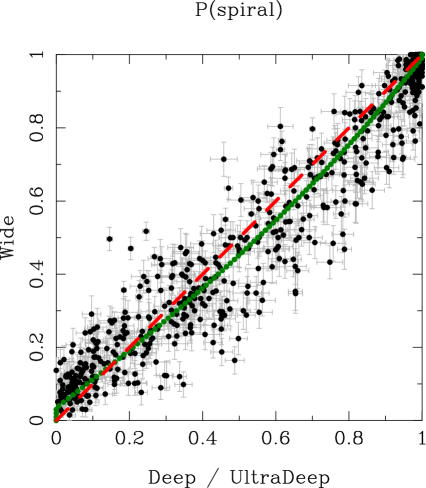
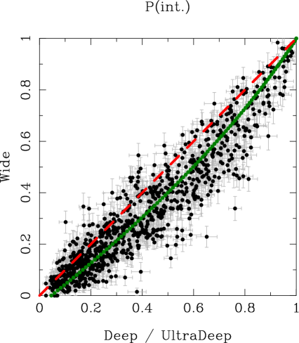
Figure 5: Left: Comparison of $P(spiral)$ between the Wide and Deep/UltraDeep layers for the same set of objects. A point is an object and the associated error bars indicate the statistical uncertainty. The dashed line is the one-to-one relationship, while the green dotted curve is the median of the distribution running over $P(spiral)$ for Wide. Right: As in the left figure but for $P(int.)$.

3.2 Redshift Dependence

Next, we look into the redshift dependence as galaxies at higher redshifts suffer more significantly from cosmological dimming. We evaluate the dependence as a function of absolute magnitude; the reduction in the angular resolution on the physical scale at high redshift likely affects faint (and small) objects more severely than bright objects and thus the effect is strongly dependent on magnitude as well. Fig. 6 shows the fractions of spiral and interacting galaxies as a function of redshift and absolute magnitude in the $r$-band. We define spiral galaxies as those with $P(spiral)>0.79$ and interacting galaxies as those with $P(int.)>0.79$ (see the next subsection for the choice of the threshold).

We first discuss the spiral fraction shown in the top panels. The spiral fraction is a function of magnitude in the sense that the spiral fraction decreases at brighter magnitudes. But, that is not our focus here as it is an intrinsic trend. We are interested in the redshift dependence. Over the narrow redshift range of $0<z<0.2$, we can reasonably assume that the intrinsic spiral fraction does not significantly change (i.e., no significant evolution since $z=0.2$). Thus, any trend with redshift can be attributed to a classification bias. Willett et al. (2013) indeed observed strong redshift dependence in Galaxy Zoo 2 (GZ2) in the sense that the spiral fraction decreases at higher redshifts and they made a statistical correction for it. Our spiral classification shows a similar but weaker trend with redshift. GALAXY CRUISE appears less biased than GZ2. This is likely because the HSC images are sufficiently deep to robustly classify bright galaxies across this redshift range (Tadaki et al., 2020). We apply only a weak correction to the spiral fraction:

$$P(spiral)_{corr}=\frac{P(spiral)}{1-0.5z},$$ (3)

where $z$ is redshift. The maximum correction factor applied is only 11%, but it does reduce the redshift trend as shown in the top-right panel of Fig. 6. Note that, when $P(spiral)_{corr}>1$, we set $P(spiral)_{corr}=1$. For reference, the correction applied in GZ2 spans over a wide range but is typically $\sim 50\%$. There is still some redshift trend left in the top-right panel in the sense that the spiral fraction is very large at $z\lesssim 0.05$. It might be due to the small volume probed. We find that there are few massive clusters at $z<0.05$, and galaxies at this redshift range are predominantly field galaxies ($\sim 1\%$ galaxies in are in dense environments). On the other hand, about 10% of galaxies at $0.05<z<0.1$ are in dense environments. We may be suffering from the morphology-density relation, which we will discuss in Section 4.2, in the top-right panel.

The bottom panels in Fig. 6 shows the interaction fraction. There is a weak redshift trend even for very bright galaxies in the sense that the interaction fraction decreases towards higher redshifts. This is expected because tidal features are often diffuse and extended and we miss those features more easily at higher redshifts. We correct for the redshift dependence in the following way:

$$P(int.)_{corr}=\frac{P(int.)}{1-z}.$$ (4)

The correction is stronger than that for the spiral fraction and the maximum correction applied is 25%. As shown in the bottom-right panel, this correction significantly reduces the redshift trend for interacting galaxies. We note that we need both the redshift and depth corrections. The former reduces the redshift dependence of our classifications and the latter changes the overall normalization of $P(spiral)$ and $P(int.)$.

We have confirmed that our main results in this paper are not affected significantly by whether or not we apply the corrections for the spiral and interaction fractions. We denote $P(spiral)_{corr}$ and $P(int.)_{corr}$ as simply $P(spiral)$ and $P(int.)$ respectively in what follows for the sake of simplicity.

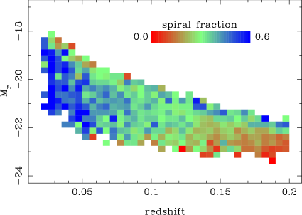
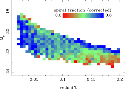
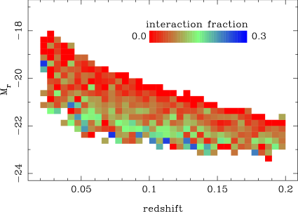
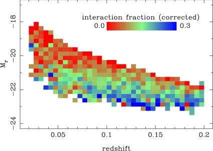
Figure 6: Fraction of spiral galaxies (top) and interacting galaxies (bottom) plotted as a function of redshift and absolute magnitude. The left is the original classification, and the right is after applying the redshift corrections (Eqs. 3 and 4 ). The color bar in each panel shows the mapping between color and fraction. Only pixels with more than 10 objects are plotted. In each panel, the upper right part is missing objects because both SDSS and GAMA are fluxed-limited survey (i.e., intrinsically fainter galaxies at higher redshifts are not targeted). The missing bottom-left part is due to the small volume probed at low redshifts.

3.3 Color-Magnitude Diagram

There may also be a bias in the participants’ classifications themselves as visual classifications are subjective. In order to reduce the subjectivity, it is a common practice to classify objects by multiple people independently (e.g., Fukugita et al. (2007)). Although this is already done in GALAXY CRUISE as we merge classifications by many participants for each galaxy (see Fig. 3), it is still useful to check if there is a systematic bias especially because the classifications are made by non-professional astronomers. However, this is not a trivial question because there is no truth table of morphology for our sample and edge-cases are difficult even for professional astronomers.

In order to roughly evaluate the classification accuracy, we use colors as the truth table. That is, we assume that elliptical galaxies are on the red sequence and spiral galaxies are in the blue cloud. There are of course green-valley galaxies, which are often bulge-dominated spiral galaxies, and also spiral galaxies are not always blue; edge-on spirals are red, and there is a population of spiral galaxies with no sign of ongoing star formation (van den Bergh, 1976; Couch et al., 1998; Masters et al., 2010; Shimakawa et al., 2022). However, there is overall a good correlation between morphology and color. For instance, Schawinski et al. (2009) showed that the vast majority ($96\%$) of the visually selected elliptical galaxies are red. Colors are a different attribute than morphology, but we use them as a proxy for morphology for now.

Fig. 7 shows the rest-frame $u-r$ color k-corrected to $z=0.1$ using the k-correction code by Blanton & Roweis (2007) plotted against absolute magnitude in the $r$-band with galaxies color-coded according to their $P(spiral)$. As can be seen, the red sequence and blue cloud are fairly well populated by elliptical and spiral galaxies, respectively. This demonstrates that the classifications are good at least to the first order. There are, however, galaxies with large $P(spiral)$ on the red sequence and those with low $P(spiral)$ in the blue cloud. Galaxies with intermediate $P(spiral)$ are located both on the red sequence and the blue cloud. They may not necessarily be wrong classifications as discussed above, but we for now assume that the colors are the truth table and make an attempt to quantify the classification accuracy below.

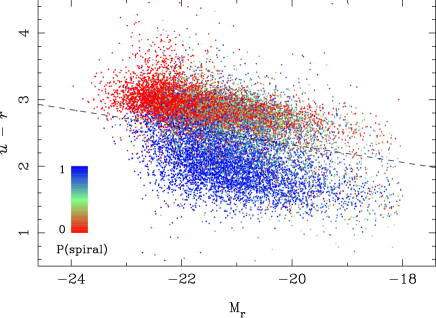
Figure 7: Rest-frame $u-r$ color plotted against $r$-band absolute magnitude. Galaxies are color-coded according to their $P(spiral)$ as shown by the color bar. We split the red/blue galaxies at the dashed line.

The left panel of Fig. 8 shows the $P(spiral)$ distributions of the red and blue galaxies. $P(spiral)$ of red galaxies is sharply peaked at $P(spiral)=0$ with a long and flat tail towards larger $P(spiral)$. The distribution of blue galaxies is similar albeit with a broader wing around $P(spiral)=1$. The tails indicate that there may be misclassifications. To better characterize it, we show in the right panel the purity and completeness of spiral galaxies as a function of threshold $P(spiral)$. Here we define purity as

$${\rm purity}=\frac{N_{blue,\ selected}}{N_{selected}},$$ (5)

where $N_{selected}$ is the number of galaxies with $P(spiral)$ above a certain threshold. The threshold here is a free parameter and is taken in the horizontal axis. $N_{blue,\ selected}$ is the number of blue galaxies among the selected galaxies. Thus, the purity is the fraction of blue galaxies among galaxies selected with a threshold $P(spiral)$. Likewise, we define completeness as

$${\rm completeness}=\frac{N_{blue,\ selected}}{N_{blue}},$$ (6)

where $N_{blue}$ is the total number of blue galaxies and $N_{blue,\ selected}$ is the number of blue galaxies with $P(spiral)$ above the threshold.

The purity shown in the right panel increases with increasing the threshold $P(spiral)$. This is expected because the contamination of elliptical galaxies decreases with more stringent $P(spiral)$ cuts. On the other hand, the completeness decreases with increasing threshold $P(spiral)$. We want to be both pure and complete, but we need to make a compromise between the two in the presence of contaminating galaxies. Here we choose to take $P(spiral)=0.79$ indicated as the vertical dashed line as the threshold. This is the point where both purity and completeness is about 75%. We have confirmed that our primary conclusions in this paper remain unchanged if we perturb the threshold within a reasonable range, e.g., $P(spiral)>0.5$.

A similar analysis will be useful for $P(int.)$, but it is more difficult because there is no truth table or even a good proxy for interaction features. Rest-frame colors or other well-measured quantities do not work as a proxy. Furthermore, interaction features are intrinsically more difficult to identify than elliptical vs spiral. Future missions with deeper and sharper imaging data over a wide area will allow us to better characterize the classification accuracy for interacting galaxies. For now, we choose to conservatively adopt the same threshold, $P(int.)>0.79$, to define interacting galaxies. Once again, we have confirmed that main conclusions of the paper are not sensitive to the particular choice of the threshold within a reasonable range. We plan to carry out a campaign to classify galaxies from cosmological hydrodynamical simulations; we visualize these simulated galaxies accounting for various observational effects and isert them to the real HSC images, so that the participants can classify them (Bottrell et al. in prep.). Because we know the merger histories of the simulated galaxies, we expect that we will be able to evaluate how well the partipants can identify interacting galaxies as functions of, e.g., mass ratio and merger phase, and discover an optimal $P(int.)$ threshold.

An approach alternative to probability thresholding adopted here is to simply use the probabilities as weights; a galaxy with $P(spiral)=0.3$ is counted as 0.3 of a spiral galaxy. Which approach to adopt depends on science applications, and we briefly discuss this point in Appendix A.

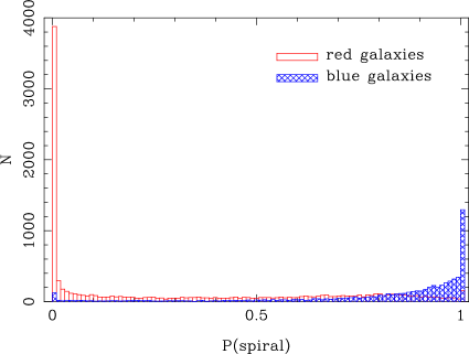
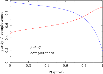
Figure 8: Left: Distribution of $P(spiral)$ for red (open histogram) and blue (shaded histogram) galaxies. Right: Purity and contamination rate plotted as a function of threshold $P(spiral)$. For instance, the purity and contamination at $P(spiral)=0.2$ are for spiral galaxies defined as $P(spiral)>0.2$. The vertical dashed line is the threshold adopted in this paper.

3.4 Gallery of Selected Objects

To visualize the participants’ classifications, we present a gallery of elliptical and spiral galaxies in Fig. 9. They are high-confidence elliptical and spiral galaxies and the classifications are indeed accurate. It will also be instructive to look at galaxies with intermediate $P(spiral)$ shown in the bottom panel. Interestingly, these objects tend to be S0-like galaxies; we do not explicitly include S0’s as a galaxy type in our classification scheme as they are difficult even for professional astronomers, but the participants’ classifications are actually useful to identify them and they are rightly classified as an intermediate type between elliptical and spiral. The color of these objects seem to be a mixture of red and blue and we find that they are indeed located on both the red sequence and blue cloud.

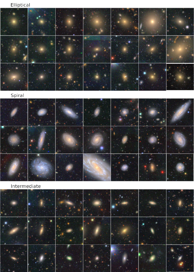
Figure 9: Top: Gallery of galaxies with $P(spiral)<0.05$ (i.e., elliptical galaxies). Each image is 1 arcmin on a side. Middle: Same as the top panel, but for spiral galaxies with $P(spiral)>0.95$. Bottom: Galaxies with $P(spiral)\sim 0.5$. These objects tend to be edge-on S0 galaxies.

Fig. 10 shows galaxies with four distinct interaction features. These galaxies are first selected as $P(int.)>0.79$ and then 21 objects with the highest probabilities for each category are shown in these figures. It is impressive that the classifications are made very well; all these individual features are nicely captured by the participants. Galaxies with distorted shapes tend to have a nearby companion, which is likely interacting with the target galaxies. We find that some of the tidal tails seem to be distorted spiral arms. It is in some cases difficult to distinguish tidal tails from distorted arms, but this tendency of misclassifying distorted arms as tidal tails is a possible classification bias in GALAXY CRUISE. As for fans/shells, coherent caustic features are observed in all cases. Finally, ring galaxies are also all nice ring galaxies. Interestingly, they are all face-on ring galaxies; there should be edge-on (or polar) ring galaxies, but they are not identified. They might be confused with linear tails. We will further discuss ring galaxies in Section 4.5.

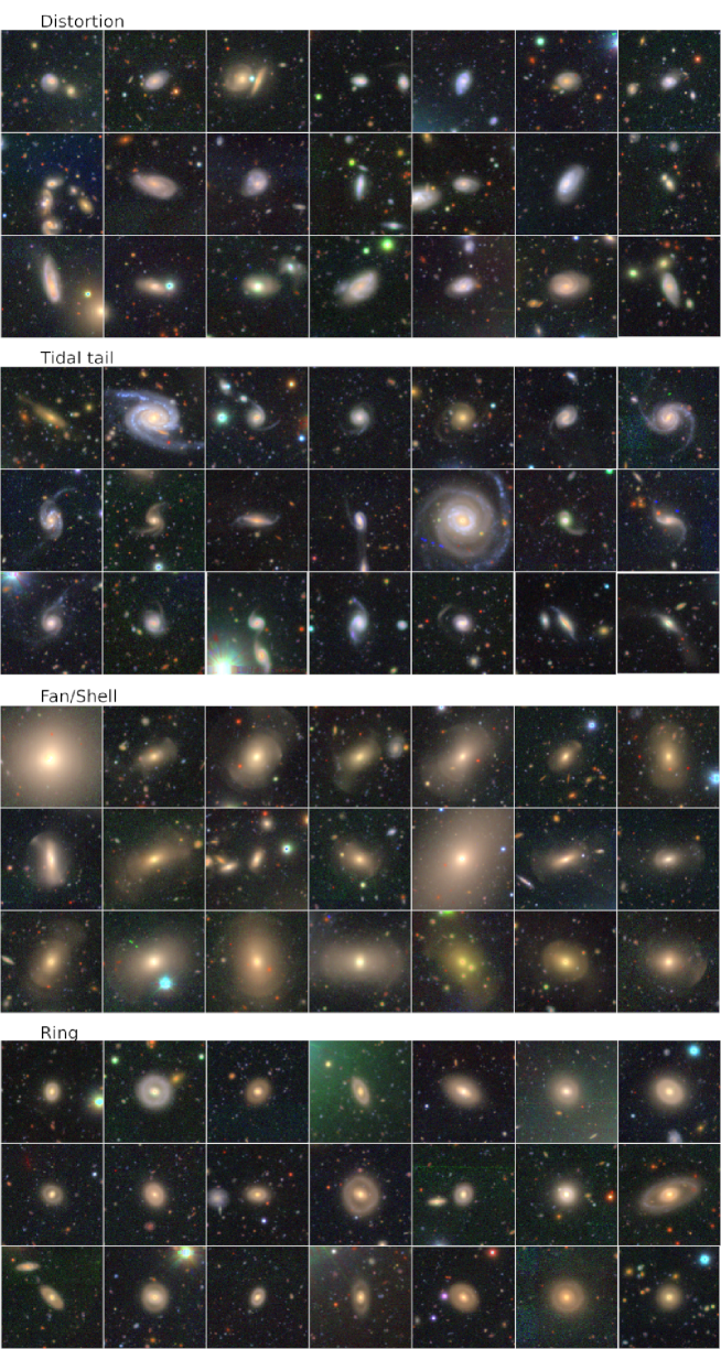
Figure 10: Gallery of interacting galaxies. Shown are those with highest probabilities for distorted shapes, tidal tails, fan/shell, and ring from top to bottom. Each panel is 1 arcmin on a side.

Let us also comment on galaxies with lower $P(int.)$. Visual inspections of a subset of $P(int.)\sim 0.5$ cases suggest that they are indeed a mixture of objects; some show a weak hint of distorted shapes, faint tails, etc, while others do not seem to exhibit clear interaction features. It seems wise to set the threshold to securely identify interacting galaxies well above 0.5 as we do in this paper. Another interesting class of objects is interacting galaxies with intermediate probabilities for invididual interaction features. We recall that we allow the participants to choose multiple interaction features because some of the features can be difficult to distinguish and some galaxies actually exhibit multiple features. Visual inspections of interacting objects with the probability of each feature between 0.15 and 0.35 indeed show complex morphologies with multiple features. Tidal tails and shells are most frequently observed, but distorted shapes and ring-like features are also observed.

Finally, we show in Fig. 11 a collection of violent mergers. This is constructed from a joint slection of $P(not\_sure)>0.2$ from the first question and $P(int.)>0.79$ from the second question. As we discussed in Section 2.4, the ’not sure’ option was not used as we intended, but a certain fraction of the participants followed our intention and sorted objects with significantly disturbed morphology into the ’not sure’ category. The mergers in the figure are all in a violent merger phase and the original morphologies of the galaxies are indeed difficult to classify. In the analyses we present in Section 4, we primarily focus on interacting galaxies defined as $P(int.)>0.79$, but we also include the violent merger subsample defined here. We note that the violent merger subsample comprises 8% of the interacting galaxy sample.

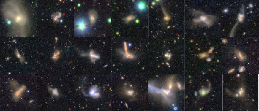
Figure 11: Galaxies with $P(int.)>0.79$ and $P(not\_sure)>0.2$. Each panel is 1 arcmin on a side.

3.5 Statistics of Interacting Galaxies

Before we discuss properties of the target galaxies in detail in the next Section, we briefly summarize statistics of interacting galaxies in Fig. 12. Overall, we find that about 13% of galaxies in our sample are interacting galaxies. The sample is not volume-limited and the number should not be over-interpreted, but the numbers here do not significantly change if we make a volume-limited sample with $z<0.1$ and $M_{r}<-20.5$. Also, the number is somewhat sensitive to the threshold $P(int.)$ value adopted (e.g., if we reduce it to 0.5, 36% of galaxies are interacting).

It is interesting to note that the abundance spiral galaxies relative to elliptical galaxies among the interacting galaxies is about 0.72 as shown in the leftmost bar, while this ratio is about 0.60 for non-interacting galaxies. The same trend holds for a volume-limited sample of $M_{r}<-20.5$ at $z<0.1$. Darg et al. (2010a) found that the spiral to elliptical fraction among interacting galaxies is about twice higher than the global population. While direct comparisons cannot be made as the parent samples are constructed in different ways, we observe a similar (but weaker) trend.

Turning to individual features, we find that tidal tails and distortions are the most common interaction features and they comprise about 3/4 of all interacting galaxies. Spiral galaxies are more abundant than ellipticals for tidal tails, and it is likely due to the misclassifications of distorted spiral arms as tails. The remaining 1/4 of the interacting galaxies is split about equally into fan and ring features. Elliptical galaxies dominate over spiral galaxies here. We suspect that this is at least partly due to the general difficulty (not only for the participants but for professional astronomers as well) of identifying fan and ring features in the presence of spiral arms. These features are much easier to identify around elliptical galaxies. We are going to look at statistical properties of galaxies in GALAXY CRUISE in the next section and we keep these biases in mind.

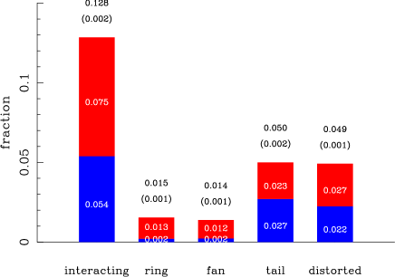
Figure 12: The leftmost bar shows the fraction of interacting galaxies among the entire sample. The number at the top of the bar and the one in the brackets are the fraction and its uncertainty. The bar is split into the red and blue parts, which represent the elliptical and spiral fractions, respectively. The remaining bars are for the ring, fan, tail, and distortion features, and they are normalized such that the sum of their abundances equals to the abundance of interacting galaxies as shown in the leftmost bar. The meaning of the numbers and the red/blue parts are the same as the leftmost one. For reference, the fractions of elliptical and spiral galaxies that are not interacting are 0.55 and 0.32, respectively (these numbers are normalized in the same way and hence the total fraction of non-interacting galaxies is 0.87).

4 Properties of Galaxies in the Local Universe Revisited

Based on the catalog constructed in the previous Section, we now move on to discuss statistical properties of the local galaxies. We first make a comparison with GZ2 (Willett et al., 2013) in Section 4.1. There is a more recent catalog based on deeper DECals data (Walmsley et al., 2022), but here we focus on GZ2 as it is the most widely used visual morphology catalog. We then turn our attention to environmental dependence of galaxy morphology in Section 4.2. In the following Section 4.3, we discuss AGNs and revisit the classic picture of AGN activities being triggered during galaxy interactions. Another activity that might be enhanced by mergers is star formation and we look into it in Section 4.4. An interesting class of objects in GALAXY CRUISE is ring galaxies; the participants’ identification of ring galaxies is accurate as shown in Fig. 10 and we discuss their statistical properties in Section 4.5. Finally, based on a number of simple assumptions, we infer the merger rate from GALAXY CRUISE and discuss the mass growth rate of galaxies in Section 4.6.

4.1 Comparison with GalaxyZoo2

We cross-match our catalog with GZ2 ’Main’ catalog (Willett et al., 2013) with positions. 8,354 objects are matched within 1.5 arcsec. We first compare classifications from GZ2 with those from GALAXY CRUISE on an object-by-object basis.

The GZ2’s classification scheme is different from ours, and there is no elliptical vs. spiral question in GZ2. However, the first question in GZ2, “Is the galaxy smooth and round with no sign of a disk?”, is sufficiently close and we use this question to compute $P(spiral)$ from GZ2. To be specific, a ’No’ to the question indicates that a galaxy is a spiral galaxy. There is a more specific question about the spiral feature later in the sequence of questions, “Is there any sign of a spiral arm pattern?”. Not all volunteers are asked this question. We could compute a conditional probability for spiral arm (Casteels et al., 2013), but we prefer to be simple here and use only the first question.

For interaction features, we use “Is there anything odd?” and the subsequent question about observable features to estimate $P(int.)$. As some of the features are not a result of interaction (e.g., dust lane), we compute $P(int.)$ as a product of $P(there\ is\ something\ odd)$ and $P(ring)+P(disturbed)+P(irregular)+P(merger)$.

We use GZ2’s classifications with weights to individual users (weighted fraction). There is a fraction corrected for the classification bias as a function of redshift (debiased fraction). However, as noted in Walmsley et al. (2022), these debiased fractions are useful only in a statistical sense and are not appropriate for object-by-object comparisons. For this reason, we focus on the weighted fraction here.

The left panel in Fig. 13 compares $P(spiral)$. There is a clump of objects at $P\sim 0$ (bottom-left corner) and 1 (top-right corner). These are objects with obvious morphology and the classifications agree well. However, there is a significant population of galaxies in the bottom-right part of the figure; GALAXY CRUISE classifies them as spiral galaxies, while GZ2 classifies them as elliptical. We randomly draw objects from the bottom-right corner and show their postage stamps in Fig. 14. All of these galaxies are clearly spiral galaxies. The reason for the discrepant classifications is simply the image quality; the SDSS images do not have sufficient depth and resolution to identify the spiral feature.

The right panel in Fig. 13 shows that there is also a significant scatter in the identifications of interacting galaxies. The top-left corner is empty and there is a large population again in the bottom-right corner. Fig. 15 shows postage stamps of randomly drawn objects from the bottom-right corner, and all these galaxies exhibit a clear feature to indicate interactions. The image depth is again the main reason for the discrepancy. These figures demonstrate that the classifications from GALAXY CRUISE are more accurate than those from GZ2.

Figure 13: Comparisons between GZ2 and GALAXY CRUISE. The left figure shows $P(spiral)$ from GZ2 plotted against that from GALAXY CRUISE. The dots are the weighted fraction from GZ2. The dashed line shows the one to one correspondence. The right figure is for $P(int.)$ and the meanings of the symbols are the same as in the left figure.

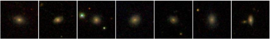
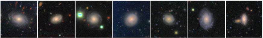
Figure 14: Randomly drawn objects with $P_{GC}(spiral)\sim 1$ and $P_{GZ2}(spiral)\sim 0$. The top row is the SDSS images used for GZ2 and the bottom row is GALAXY CRUISE for the same objects. Each image is 48 arcsec on a side.

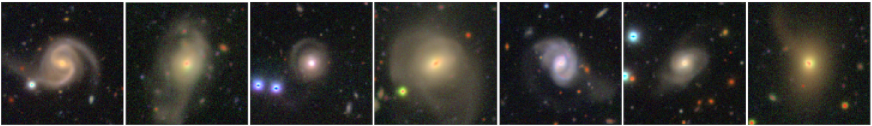
Figure 15: As in Fig. 14 but for interacting galaxies.

Finally, we look at the fraction of spiral galaxies and interacting galaxies as a function of absolute magnitude in Fig. 16. We recall that we define spiral galaxies as galaxies with $P(spiral)>0.79$. We adopt the same definition also for GZ2 to be fair. The left panel shows the well-known trend that the intrinsically bright ($\sim$ massive) galaxies tend to be early-type galaxies, while faint galaxies are more populated by late-type galaxies. The overall normalization of the spiral fraction is different between GALAXY CRUISE and GZ2 in the sense that the spiral galaxies are more abundant in GALAXY CRUISE. This trend holds even when we use the debiased fraction from GZ2 (we use the debiased fraction here because this is a statistical comparison). We note that, if we define spiral galaxies as those with $P(spiral)>0.5$, GALAXY CRUISE and GZ2 debiased fractions are in good agreement, except for the magnitude range at $M_{r}\gtrsim-21$, where GZ2 falls below GALAXY CRUISE. Baldry et al. (2004) examined the relative abundance of red and blue galaxies in the local Universe and showed that the fraction of red galaxies rises slowly from $M_{r}=-18$ to $-22$, and then sharply rises to almost unity at the brightest magnitudes. While we plot the spiral fraction ($\sim$ fraction of blue galaxies) in Fig. 16, the trend in the figure is fully consistent with the finding by Baldry et al. (2004). Colors are a different property from morphology as noted earlier, but the agreement here is reassuring because this strongly suggests that the participants’ classifications are accurate.

The right panel shows the fraction of interacting galaxies. We recall again that the interacting galaxies are conservatively defined as those with $P(int.)>0.79$ and the same definition is used for GZ2. The same trend as in the left panel can be seen; the interaction fraction is higher in GALAXY CRUISE. Interestingly, the weighted fraction and debiased fraction both yield similarly low fractions. The fractions remain low even if we define interacting galaxies as $P(int.)>0.5$.

GALAXY CRUISE’s interaction fraction seems to show a declining trend with magnitudes; fainter galaxies are less likely to exhibit interaction features. This luminosity dependence is consistent with previous work (e.g., Patton & Atfield (2008)). It is also consistent with Rodriguez-Gomez et al. (2015) who examined the major merger rate in the Illustris Simulation (Genel et al., 2014; Vogelsberger et al., 2014) and showed that the rate is a strong function of stellar mass in the sense that more massive galaxies experience more mergers. The mass dependence of merger rate indicates that more massive galaxies have a larger fraction of accreted (ex-situ) stars (Rodriguez-Gomez et al., 2016). Our result here points to the same picture.

As described in Section 2.3, we mistakenly used HSC photometry to select targets. A preliminary analysis of the data from the 2nd season shows that we tend to miss spiral galaxies and interacting galaxies from the sample because they have significant structure. The spiral and interaction fractions discussed here should thus be interpreted as a lower limit. The ongoing 2nd season of GALAXY CRUISE will get rid of this problem and give us better estimates of these fractions.

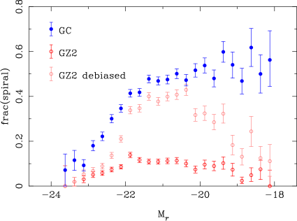
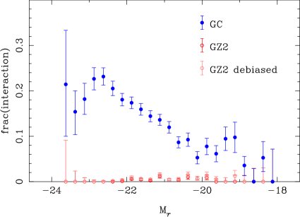
Figure 16: Left: Fraction of spiral galaxies plotted against $r$-band absolute magnitude. The blue filled circles are GALAXY CRUISE (GC), and the open circles are GZ2. For GZ2, we show the spiral fraction using the weighed fraction (red) and debiased fraction (pink). The error bars show the Poisson uncertainty. Right: Fraction of interacting galaxies as a function of the $r$-band absolute magnitude. The meaning of the symbols are the same as in the left panel.

4.2 Dependence on Environment

Another interesting question about our targets is their environmental dependence. We characterize their local environment and discuss how the spiral fraction and interaction fraction change with environment. The former is the well-known morphology-density relation (Dressler, 1980) and we first check if the participants’ classification can reproduce it.

To compute the local environment, we use spectroscopic redshifts from SDSS and construct a volume-limited sample at $z<0.1$ with $M_{r}<-20.5$. We then estimate a distance to the 5th nearest neighbor within a radial velocity slice of $\pm 1000\rm\ km\ s^{-1}$ from each of our target, and translate it into local density as $5/(\pi r_{5}^{2})$, where $r_{5}$ is the projected physical distance to the 5th-nearest neighbor. We apply the same redshift and magnitude cuts to our targets.

The left panel of Fig. 17 shows the fraction of spiral galaxies as a function of local density. We observe the spiral fraction decreasing with increasing local density. In the densest region, the spiral fraction is below 20%. We observe a hint of a break in the relation at $density\sim 2\ \rm Mpc^{-2}$, above which the fraction decreases more rapidly. The break density corresponds to the virial radius of groups and clusters (Tanaka et al., 2004). The participants’ classifications nicely reproduce the morphology-density relation.

The right panel of Fig. 17 shows the fraction of interacting galaxies as a function of local density. We observe a decreasing trend with increasing local density as in the spiral fraction, although the scatter is larger. The trend remains the same with different bin sizes. The classical idea about interactions is that group environments is an efficient place for interactions because relative velocities between galaxies is not very high, while more massive clusters are not very efficient due to their high velocities. This idea is supported by numerical simulations (Jian et al., 2012). The local density alone cannot distinguish groups from clusters (Tanaka et al., 2004) and we have a mix of groups and clusters in Fig. 17. Our result here implies that interactions occur, on average, less frequently in high density regions.

This possible decreasing trend is not consistent with some of the previous studies (e.g., Lin et al. (2010); de Ravel et al. (2011)), which reported an increasing fraction of interacting galaxies with increasing local density. One might suspect that the difference is potentially due to different environments probed. Some of the previous work is based on a relatively small data set such as zCOSMOS (Lilly et al., 2007) and DEEP2 (Newman et al., 2013), and thus their interacting galaxies are mostly located in groups rather than in clusters. On the other hand, we use a larger data set and we have a larger fraction of cluster galaxies. As a quick check, we perform the same analysis as in Fig. 17 with density estimated with the 20th nearest neighbor so that we are more sensitive to large-scale environment. We find that the same trend holds; the interaction fraction decreases in high density environments. This suggests that the dominance of groups vs. clusters is not the main driver of the observed trend. We also examine the distribution of the violent mergers (Section 3.4) but they do not seem to prefer any specific environment.

The difference is at least in part due to different methods employed to identify interacting galaxies. Many of the previous studies are based on galaxy pairs, which probe the pre-merger phase, while our work is based on visual signatures of interactions, which are also sensitive to later phases of interactions. Also, it is possible that the timescale over which tidal features are observable depends on environment. For instance, many galaxies are traveling fast in a small volume in clusters, tidal features may be short-lived compared to those around isolated galaxies. We speculate the combination of these reasons may be able to explain the observed difference. The error bars in Fig. 17 are still large and an increased sample of interacting galaxies from, e.g., machine-learning based on the GALAXY CRUISE classifications will allow us to further explore the origin of the reduced frequency of interactions in dense regions.

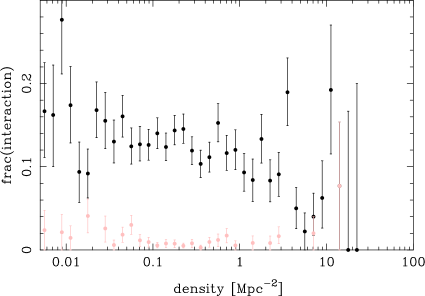
Figure 17: Left: Morphology-density relation. The fraction of spiral galaxies is plotted against local density. Only bins with more than 5 objects are plotted. Right: Fraction of interacting galaxies as a function of local density. The pink symbols are for the violent merger subsample.

4.3 AGN fraction

Next, we look into the long-standing question of whether galaxy-galaxy interactions trigger AGN activities (Keel et al., 1985). AGNs can be identified by a variety of methods, e.g., X-rays, IR colors, variability, etc. As all of our targets have spectra from SDSS and GAMA, we use emission line intensity ratios suggested by Baldwin et al. (1981). In order to separate AGNs from star forming galaxies, we use the threshold proposed by Kauffmann et al. (2003). This diagnostics involve 4 emission lines: H$\beta$, [OIII] ($\lambda 5007$), [NII] ($\lambda 6583$), and H$\alpha$. We require that all of these 4 lines are measured at $>3\sigma$. Among 20,686 galaxies GALAXY CRUISE targeted, 7,994 galaxies passed the condition. The other galaxies are considered normal (i.e., non-AGN host) galaxies, although some of them may harbor obscured or very weak AGNs.

To get a rough picture of the AGN population in our sample, we first show in Fig. 18 the fraction of AGNs as a function of magnitude. The exact AGN fractions here should be taken with caution because they are not from a volume-limited sample. Nonetheless, relative differences between the interacting and non-interacting galaxies are interesting; AGN fraction is consistently higher for interacting galaxies than for non-interacting galaxies at relatively bright magnitudes ($M_{r}\lesssim-21$), while the fraction is consistent at fainter magnitudes. This trend is not sensitive to a particular choice of the bin size. The observed higher AGN fraction among interacting galaxies is in qualitative agreement with Ellison et al. (2013), who observed that AGNs are more common in galaxy pairs with smaller angular separations. We see a hint of the very high AGN fraction among bright violent mergers, which may also be in line with Ellison et al. (2013) as the closest pairs are more likely to be strongly disturbed. Goulding et al. (2018) addressed the AGN enhancement using the HSC-SSP imaging data and found that AGNs are a factor of $2-8$ times more abundant. While the differences in the way mergers and AGNs are identified again make it difficult to make quantitative comparisons, we are in qualitative agreement.

We then make an attempt to see whether any of the specific interaction features is more important for triggering AGN activities. Fig. 19 shows AGN fractions for each interaction feature for a volume-limited sample with $z<0.1$ and $M_{r}<-20.5$. We find that the AGN fraction is clearly higher among interacting galaxies; 35% of interacting galaxies exhibit a sign of AGN, while the fraction is 28% for non-interacting galaxies. This suggests that interactions can indeed trigger AGN activities at a certain rate. If we turn our attention to individual interaction features, we find that the relative fractions of fan, tail, and distortion features to the total AGN fraction are similar to the overall feature fractions shown in Fig. 12; tail and distortions are about the same fraction and their sum comprises about 3/4 of the interacting galaxies, and the ring and fan features are about one-third of each of these features. A possible interpretation is that the orbital parameters of infalling galaxies are not important for triggering AGN activities. It may simply be the tidal disturbance that induces AGN activities. We note that our interaction galaxies include many phases of mergers and interactions; some are in pre-merger phases, while others are post-mergers. There may be phase dependence of AGN activities; in fact, the violent mergers (Section 3.4) seem to show a higher AGN fraction of $0.42\pm 0.07$, indicating that the strong tidal field may be the key to trigger AGNs. The uncertainty is large at this point, and more detailed investigations of merger phases may shed further light on the physical process to activate AGNs.

Our analysis makes it clear that galaxy-galaxy interactions can trigger AGN activities, but galaxies without any clear sign of interactions also exhibit AGN activities and their fraction is as high as 28%. This suggests that interactions are not the only mechanisms to trigger AGNs, and secular processes are one of the primary ways to activate AGNs. Ellison et al. (2019) reported that IR-selected AGNs show a sign of disturbance more frequently than optically-selected AGNs. It would be interesting to look at AGNs selected in various ways and investigate this issue further. We leave it for future work.

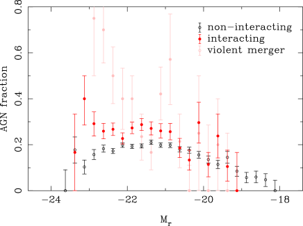
Figure 18: AGN fraction plotted against $r$-band absolute magnitude. The red and black circles for interacting and non-interacting galaxies, respectively. The pink points are the violent merger subsample. The error bars show the Poisson errors. Only bins with more than 5 objects are plotted here.

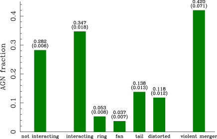
Figure 19: Fraction of AGNs for interacting and non-interacting galaxies (left two bars). The overall AGN fractions are higher than those shown in Fig. 18, but here we use a volume-limited sample at $z<0.1$. Interacting galaxies are split into different features as shown in the following four bars to the right. These feature fractions are normalized such that the sum of each feature equals the AGN fraction (i.e., the sum is 0.347). The rightmost bar is the violent merger subsample. The numbers on the top of each bar are the fraction and its statistical uncertainty, respectively.

4.4 SFR enhancement during interaction

Another activity that may be enhanced during interactions is star formation (e.g., Nikolic et al. (2004); Ellison et al. (2008, 2013)) and we focus on star formation activities of interacting vs. non-interacting galaxies in this subsection. There are multiple ways to infer SFRs of galaxies, but here we adopt the one based on the H$\alpha$ luminosity. We translate the H$\alpha$ luminosity into SFR using the relationship from Murphy et al. (2011). We correct for the dust attenuation when H$\beta$ is measured at $>3\sigma$ using the Cardelli et al. (1989) dust attenuation curve. No correction is made for objects with weaker H$\beta$. We apply no correction for the fiber aperture loss as we are interested in relative differences between interacting and non-interacting galaxies.

SFR is known to correlate significantly with stellar mass (Brinchmann et al., 2004). As the interaction fraction is a function of absolute magnitude (and stellar mass as well) as shown in Fig. 16, a direct comparison of SFRs is not easy to interpret. We utilize the fact that the SFR-$M_{*}$ correlation is roughly linear (Speagle et al., 2014) and we compare the distributions of specific SFR (sSFR) defined as SFR$/M_{*}$. The relation is not completely linear, but we have confirmed the small non-linearity does not alter our conclusion here. We use stellar mass estimates from Ahn et al. (2014) (’GranadaWideDust’) for SDSS galaxies. We exclude the GAMA galaxies to avoid potential systematic effects arising from different stellar mass estimates, but the fraction of GAMA galaxies is only $\sim 10$% of the entire sample (Section 2.3) and whether we include them or not does not change our results.

Fig. 20 shows the sSFR distributions of the two populations. For the non-interacting galaxies, we construct a mass-matched sample; we randomly draw a subset of non-interacting galaxies so that their stellar mass distribution is consistent with that of interacting galaxies. The plot is for the entire sample, but the plot remains similar if we use a volume-limited sample with $z<0.1$ and $M_{*}>10^{10.5}\ M_{\odot}$. Note that AGNs identified in the previous subsection are excluded from the figure so that we do not misinterpret AGN emission as star formation activity. Note as well that we focus on spiral galaxies with $P(spiral)>0.79$ because we are interested in the enhancement of star formation activities. We confirm that elliptical galaxies in our sample do not exhibit a significant sSFR enhancement.

The sSFR distributions are clearly different; interacting galaxies show an sSFR enhancement by about a factor of 2. The overall shapes of the distributions are similar, but there is a clear offset between them (the median offset is 0.31 dex). This enhancement is consistent with the finding by Darg et al. (2010b), Ellison et al. (2013), Bickley et al. (2022) among others, although their interacting galaxies are selected in different ways. The enhancement is also consistent with recent hydrodynamical simulations Hani et al. (2020). As we have classifications of various tidal features, we can address which feature is more important. It seems the offset is primarily driven by galaxies with tidal tails. Galaxies with distorted shapes also contribute to the overall trend. Statistics is too poor for galaxies with ring and fan features to draw any conclusions about them. As noted earlier, machine-learning techniques based on the current sample will be able to make a larger sample, which will allow us to more securely characterize the relative contribution of each feature. However, it is fairly robust already from the current sample that sSFR is boosted by a factor of $\sim 2$ by interactions. Interestingly, the violent mergers (Section 3.4) show an even larger boost of a factor of $\sim 6$ (0.8 dex), indicating that both star formation and AGN activities (see the previous Section) are most significantly enhanced during the violent merger phase.

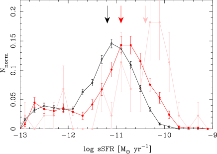
Figure 20: Specific SFR distributions of interacting (red) and non-interacting (black) spiral galaxies. The violent merger subsample is shown in pink. The error bars show the Poisson error. The arrows indicate the median of the distribution (-11.19, -10.88, and -10.39 for non-interacting, non-interacting, and violent mergers, respectively).

4.5 Ring Galaxies

Few & Madore (1986) introduced two classes of ring galaxies: O-type, which is a smooth and regular ring with galaxy nucleus at its center, and P-type, which is often knotted, asymmetric ring and the nucleus is not necessarily at the center. It is interesting that the ring galaxies shown in Fig 10 are mostly O-type rings. Some of them might be pseudo-rings (Shimakawa et al., 2022) and there is certainly a bias towards face-on rings in our classifications because there is no, e.g., polar-ring galaxy. This is at least in part due to limited resolution of our imaging data on the physical scale (our sample extends out to $z=0.2$). Buta (2017) discussed biases in ring galaxies selected from GZ2 and made a similar finding; most ring galaxies are those with bright, large outer rings with nearly face-on configuration. While our resolution is better than SDSS on which GZ2 is based, our sample likely suffers from the same bias. However, the subdominance of P-type rings is still interesting; if there were P-type rings of similar angular sizes, they would have been identified. Of course, we cannot deny the possibility that the subdominance of P-type rings is due to classification bias that it is easier for the participants to identify smooth and symmetric O-type rings. This caveat should be kept in mind.

Elagali et al. (2018) examined ring galaxies from the EAGLE simulation (Schaye et al., 2015). They found that about 80% of the ring galaxies originate from interactions. Interestingly, their ring galaxies seem to be mostly P-type rings. This may be expected as collisional rings may show star formation activities induced by the collision. The dominance of O-type rings in our sample is in contrast to their result. We visually inspect galaxies with $P(int.)>0.79$ and $P(ring)>0.5$ and find that P-type rings comprise only about 10%. We further find that more than 80% of the ring galaxies are classified as red galaxies on the basis of the color-magnitude diagram, and the remaining galaxies tend to be located in the green valley. This indicates that most ring galaxies are not actively forming stars. O-type rings can be formed by resonances due to the central bar, and the observed red color may be consistent with the secular formation mechanism. However, many of the ring galaxies in our sample do not seem to exhibit a clear bar structure. Elagali et al. (2018) found that about 20% of the ring galaxies hold the ring structure for as long as 2 Gyr or more. As our imaging data are fairly deep, we may be preferentially detecting these long-lived rings, in which star formation activities have already ceased.

In any case, more detailed investigations are clearly needed to go beyond these speculations. For instance, close comparisons with recent hydro-dynamical simulation will be useful. Also, machine-learning techniques make it possible to identify galaxies in simulations that look similar to a given observed galaxy. By identifying counterparts of the ring galaxies in simulations and go back in time, we will be able to get a better handle on the origin of these galaxies.

4.6 Merger Rate

Finally, we discuss the merger rate. It is not trivial to estimate the merger rate from our data due to a number of observational complexities; our interacting galaxies include both pre- and post-mergers, some of them might be undergoing fly-by interaction and will not merge, etc. Here, we make simplified assumptions and attempt to make a rough estimate of the merger rate.

We infer merge rate as

$$dN_{merger}=\frac{f_{int.}}{T}dt,$$ (7)

where $f_{int.}$ is the observed interaction fraction and $T$ is the typical timescale over which the interaction features can be observed with our data. Some of the merger features we have identified may be due to multiple merger events, but we assume that they are due to a single event for simplicity.

It is difficult to make a robust estimate of $T$ as the survival time of interaction features depend, for instance, on orbital parameters of infalling galaxies. A radial tail is likely short-lived because it can be destroyed as it passes through the strong tidal field around the potential center, while tangential tails (arcs) may live longer. There may also be environmental dependence as we discussed earlier. We assume that interaction features are observable for of order the dynamical timescale, $T\sim 1$ Gyr. Equation 7 is then

$$dN_{merger}=f_{int.}\left(\frac{1Gyr}{T}\right)\frac{dt}{Gyr}.$$ (8)

The inferred merger rate is shown in Fig. 21 for a volume-limited sample with $z<0.1$ and $M_{*}>10^{10.5}\rm M_{\odot}$. For comparison, we show predictions from the Illustris simulation (Rodriguez-Gomez et al., 2015). The merger rate is a strong function of mass ratio between merging galaxies in the sense that minor mergers are more common than major mergers. Here, we find that our merger rate corresponds approximately to $\mu>0.04$ (i.e., mass ratios larger than $\sim 1/25$). This large mass ratio may not be too surprising because our imaging is very deep and is able to detect faint features due to minor mergers. Note that the overall normalization of our merger rate is sensitive to the assumptions employed and it should be regarded only as a rough estimate.

Based on the merger rate, we can infer the mass growth rate as

$$\frac{dM_{1}}{dt} = <M_{2}>\frac{dN_{merger}}{dt}$$

$$\frac{dM_{1}}{M_{1}} = f_{int.}\left(\frac{<M_{2}>}{M_{1}}\right)\left(\frac{1Gyr}{T}\right)\frac{dt}{Gyr},$$ (9)

where $M_{1}$ is the mass of the central galaxy, and $<M_{2}>$ is the typical mass of an accreting galaxy. For $f_{int.}=0.13$ (which is the interaction fraction at $M_{*}=10^{11}\rm\ M_{\odot}$) and $<M_{2}>/M_{1}=0.04$, the (fractional) growth rate inferred here is $dM_{1}/M_{1}\sim 0.005\rm\ Gyr^{-1}$, which is more than an order of magnitude smaller than that estimated by Tal et al. (2009). One of the main differences is in $f_{int.}$; Tal et al. (2009) find that 70% of galaxies they observed show a sign of interaction, while we find 13%. As noted earlier, the overall normalization has a significant uncertainty both in our work and also in Tal et al. (2009) and we do not peruse the difference further at this point.

Assuming the redshift evolution of the merger rate from Rodriguez-Gomez et al. (2015) and consider all mergers with mass ratio larger than $0.04$, we expect the mass growth of a factor of $\sim 1.4$ since $z=1$ for galaxies with $M_{*}=10^{11}\rm M_{\odot}$ at $z=0$. This is in broad agreement with Davidzon et al. (2017) who evaluated the evolution of the stellar mass function of galaxies and found the observed growth of the characteristic stellar mass since $z\sim 1$ is $\sim 0.2$ dex.

Despite the simplified assumptions employed, the inferred mass growth rate roughly reproduces the observed mass growth. Our approach here is complementary to many of the literature results based on galaxy pairs (e.g., Bundy et al. (2009); López-Sanjuan et al. (2013)) due to different systematic effects. Our merger rates are, however, sensitive to the assumptions employed as well as the adopted threshold to define interacting galaxies, $P(int.)$. As we discussed in Section 3.3, we do now know the best $P(int.)$ to cut at. The adopted threshold is rather conservative and more optimal threshold may change the overall normalization.

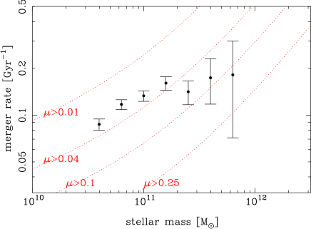
Figure 21: Merger rate plotted against stellar mass. The points show the observed merger rate inferred from Equation 8. The associated error bars include only the Poisson error. The dotted curves are from Rodriguez-Gomez et al. (2015) based on the Illustris simulation. The different curves mean different range of mass ratios ($\mu$) between the merging galaxies considered. For instance, the curve for $\mu>0.1$ is for all mergers with mass ratio of 0.1 or larger.

5 Summary

We have presented our community science project GALAXY CRUISE and its first science results. We focus on morphologies of nearby galaxies with spectroscopic redshifts from SDSS and GAMA with an emphasis on interaction features. The combination of the depth, seeing, and wide area coverage of the HSC-SSP data surpasses the previous community science projects on similar subjects; we are able to identify spiral features and interaction features that were missed in previous projects. After careful screening and statistical corrections to the classifications, the catalog is ready for various scientific explorations.

We have first compared with previous results from GZ2. We confirm that we make more accurate morphological classifications of galaxies than the previous work thanks to the better imaging data. We successfully reproduce the morphology-density relation. We find that tidal tails and distortion are the most frequently observed interaction features and they comprise about 3/4 of all the interaction features. The remainder is equally shared between the ring and fan features. The interacting galaxies seem to decrease in high density regions, which is not necessarily consistent with previous findings. We suspect that the different methods to used identify interacting galaxies can at least partly explain the difference.

As all of our targets have spectra, we apply the BPT diagnostics to identify AGNs. We demonstrate that interactions can trigger AGN activities; the fraction of AGN host galaxies among interacting galaxies is clearly higher than that of non-interacting galaxies. However, about a quarter of non-interacting galaxies harbor AGNs, which indicate that interactions are not the only mechanism to trigger AGNs. We also demonstrate that interactions enhance star formation activities of spiral galaxies by about a factor of 2. Both AGN and star formation activities are even more enhanced among violent mergers, indicating that the strong tidal field is driving this enhancement.

Finally, we have made an attempt to infer the merger rate. We find that our merger rate is similar to that inferred from the Illustris simulation for mass ratios greater than 1:25. The inferred mass growth rate due to mergers since $z=1$ is in good agreement with the observed evolution of the stellar mass function since $z=1$. As many of the previous studies inferred the merger rate from pair statistics, our analysis in this paper is highly complementary because interacting galaxies are identified in a different way.

This work is based on classifications collected during the 1st season of GALAXY CRUISE. We make the merged catalog used in the paper publicly available at the GALAXY CRUISE website, so that the world-wide community benefits from the large number of high-quality classifications. As emphasized throughout the paper, the HSC-SSP images are much deeper than those adopted in previous projects on similar subjects. Our catalog here can be used as a training data set to develop machine-learning algorithms and apply them to galaxies that are not targeted in this paper (e.g., those without spectroscopic redshifts and those covered in releases after PDR2), which will significantly increase the sample of interacting galaxies. This is just one example to use the catalog, and it can be used for a wide variety of purposes.

Currently, the 2nd season of GALAXY CRUISE is under way. Given the good classification accuracy achieved in the 1st season, we choose to include fainter galaxies. We also eliminate the photometry problem that was erroneously introduced. The 2nd season data will thus extend the magnitude range and help us unveil the nature of fainter galaxies in the local Universe. We will report on updated analyses using the 2nd season data in our future paper, and the classifications will be released to the community in due course as well.

This paper is based on morphological classifications of galaxies by the GALAXY CRUISE volunteers, without whom the work would not have been possible. We deeply appreciate their efforts and contributions. We thank Miraikan, the National Museum of Emerging Science and Innovation, for their support and assistance during the public experiments. The experiments were essential for us to define the classification scheme and and make a tutorial course. This work is supported by JSPS KAKENHI Grant Numbers JP 22H01270 and JSPS 22K14078. We thank the anonymous referee for constructive comments, which helped improve the paper.

The Hyper Suprime-Cam (HSC) collaboration includes the astronomical communities of Japan and Taiwan, and Princeton University. The HSC instrumentation and software were developed by the National Astronomical Observatory of Japan (NAOJ), the Kavli Institute for the Physics and Mathematics of the Universe (Kavli IPMU), the University of Tokyo, the High Energy Accelerator Research Organization (KEK), the Academia Sinica Institute for Astronomy and Astrophysics in Taiwan (ASIAA), and Princeton University. Funding was contributed by the FIRST program from Japanese Cabinet Office, the Ministry of Education, Culture, Sports, Science and Technology (MEXT), the Japan Society for the Promotion of Science (JSPS), Japan Science and Technology Agency (JST), the Toray Science Foundation, NAOJ, Kavli IPMU, KEK, ASIAA, and Princeton University.

This paper is based on data collected at the Subaru Telescope and retrieved from the HSC data archive system, which is operated by Subaru Telescope and Astronomy Data Center at NAOJ. Data analysis was in part carried out with the cooperation of Center for Computational Astrophysics at NAOJ. We are honored and grateful for the opportunity of observing the Universe from Maunakea, which has the cultural, historical and natural significance in Hawaii.

This paper makes use of software developed for Vera C. Rubin Observatory. We thank the Rubin Observatory for making their code available as free software at http://pipelines.lsst.io/.

The Pan-STARRS1 Surveys (PS1) and the PS1 public science archive have been made possible through contributions by the Institute for Astronomy, the University of Hawaii, the Pan-STARRS Project Office, the Max-Planck Society and its participating institutes, the Max Planck Institute for Astronomy, Heidelberg and the Max Planck Institute for Extraterrestrial Physics, Garching, The Johns Hopkins University, Durham University, the University of Edinburgh, the Queen’s University Belfast, the Harvard-Smithsonian Center for Astrophysics, the Las Cumbres Observatory Global Telescope Network Incorporated, the National Central University of Taiwan, the Space Telescope Science Institute, the National Aeronautics and Space Administration under Grant No. NNX08AR22G issued through the Planetary Science Division of the NASA Science Mission Directorate, the National Science Foundation Grant No. AST-1238877, the University of Maryland, Eotvos Lorand University (ELTE), the Los Alamos National Laboratory, and the Gordon and Betty Moore Foundation.

Funding for the Sloan Digital Sky Survey IV has been provided by the Alfred P. Sloan Foundation, the U.S. Department of Energy Office of Science, and the Participating Institutions.

SDSS-IV acknowledges support and resources from the Center for High Performance Computing at the University of Utah. The SDSS website is www.sdss4.org.

SDSS-IV is managed by the Astrophysical Research Consortium for the Participating Institutions of the SDSS Collaboration including the Brazilian Participation Group, the Carnegie Institution for Science, Carnegie Mellon University, Center for Astrophysics — Harvard & Smithsonian, the Chilean Participation Group, the French Participation Group, Instituto de Astrofísica de Canarias, The Johns Hopkins University, Kavli Institute for the Physics and Mathematics of the Universe (IPMU) / University of Tokyo, the Korean Participation Group, Lawrence Berkeley National Laboratory, Leibniz Institut für Astrophysik Potsdam (AIP), Max-Planck-Institut für Astronomie (MPIA Heidelberg), Max-Planck-Institut für Astrophysik (MPA Garching), Max-Planck-Institut für Extraterrestrische Physik (MPE), National Astronomical Observatories of China, New Mexico State University, New York University, University of Notre Dame, Observatário Nacional / MCTI, The Ohio State University, Pennsylvania State University, Shanghai Astronomical Observatory, United Kingdom Participation Group, Universidad Nacional Autónoma de México, University of Arizona, University of Colorado Boulder, University of Oxford, University of Portsmouth, University of Utah, University of Virginia, University of Washington, University of Wisconsin, Vanderbilt University, and Yale University.

GAMA is a joint European-Australasian project based around a spectroscopic campaign using the Anglo-Australian Telescope. The GAMA input catalogue is based on data taken from the Sloan Digital Sky Survey and the UKIRT Infrared Deep Sky Survey. Complementary imaging of the GAMA regions is being obtained by a number of independent survey programmes including GALEX MIS, VST KiDS, VISTA VIKING, WISE, Herschel-ATLAS, GMRT and ASKAP providing UV to radio coverage. GAMA is funded by the STFC (UK), the ARC (Australia), the AAO, and the participating institutions. The GAMA website is http://www.gama-survey.org/ .

Using probabilities as weights

In the main body of the paper, we define galaxies with $P(spiral)>0.79$ as spiral galaxies. Instead of thresholding the probability, one can consider simply using the probability as weight. For instance, a galaxy with $P(spiral)=0.3$ can be counted as 0.3 spiral galaxy. Which approach to adopt depends on what one wishes to look at, but we here briefly discuss how the spiral fraction changes between the two approaches. Fig. 22 shows the spiral fraction as a function of $M_{r}$ using $P(spiral)$ as weight. This figure can be compared with Fig. 16, which is based on thresholding. Overall, the spiral fraction from GALAXY CRUISE does not change significantly. This is not surprising because $P(spiral)$ is sharply peaked at 0 and 1 as shown in Fig. 8 and thresholding at $P(spiral)=0.79$ simply splits these peaks into two. On the other hand, $P(spiral)$ from GZ2 is more contiguous, and both weighted and debiased fractions increase when $P(spiral)$ is used as weight. The debiased fractions are in better agreement with GALAXY CRUISE, but there is still the under-abundance of faint spirals.

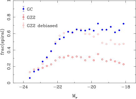
Figure 22: Same as Fig. 16, but here $P(spiral)$ is used as a weight instead of thresholding $P(spiral)$ to define spiral galaxies.

References

- Abraham et al. (1994) Abraham, R. G., Valdes, F., Yee, H. K. C., & van den Bergh, S. 1994, ApJ, 432, 75
- Abraham et al. (2003) Abraham, R. G., van den Bergh, S., & Nair, P. 2003, ApJ, 588, 218
- Aguado et al. (2019) Aguado, D. S., Ahumada, R., Almeida, A., et al. 2019, ApJS, 240, 23
- Ahn et al. (2014) Ahn, C. P., Alexandroff, R., Allende Prieto, C., et al. 2014, ApJS, 211, 17
- Aihara et al. (2018a) Aihara, H., Armstrong, R., Bickerton, S., et al. 2018a, PASJ, 70, S8
- Aihara et al. (2018b) Aihara, H., Arimoto, N., Armstrong, R., et al. 2018b, PASJ, 70, S4
- Aihara et al. (2019) Aihara, H., AlSayyad, Y., Ando, M., et al. 2019, PASJ, 71, 114
- Baldry et al. (2004) Baldry, I. K., Glazebrook, K., Brinkmann, J., et al. 2004, ApJ, 600, 681
- Baldwin et al. (1981) Baldwin, J. A., Phillips, M. M., & Terlevich, R. 1981, PASP, 93, 5
- Bickley et al. (2022) Bickley, R. W., Ellison, S. L., Patton, D. R., et al. 2022, MNRAS, 514, 3294
- Blanton & Roweis (2007) Blanton, M. R., & Roweis, S. 2007, AJ, 133, 734
- Bosch et al. (2018) Bosch, J., Armstrong, R., Bickerton, S., et al. 2018, PASJ, 70, S5
- Bottrell et al. (2019) Bottrell, C., Simard, L., Mendel, J. T., & Ellison, S. L. 2019, MNRAS, 486, 390
- Brinchmann et al. (2004) Brinchmann, J., Charlot, S., White, S. D. M., et al. 2004, MNRAS, 351, 1151
- Bundy et al. (2009) Bundy, K., Fukugita, M., Ellis, R. S., et al. 2009, ApJ, 697, 1369
- Buta (2017) Buta, R. J. 2017, MNRAS, 471, 4027
- Cardelli et al. (1989) Cardelli, J. A., Clayton, G. C., & Mathis, J. S. 1989, ApJ, 345, 245
- Casteels et al. (2013) Casteels, K. R. V., Bamford, S. P., Skibba, R. A., et al. 2013, MNRAS, 429, 1051
- Chambers et al. (2016) Chambers, K. C., Magnier, E. A., Metcalfe, N., et al. 2016, arXiv e-prints, arXiv:1612.05560
- Couch et al. (1998) Couch, W. J., Barger, A. J., Smail, I., Ellis, R. S., & Sharples, R. M. 1998, ApJ, 497, 188
- Darg et al. (2010a) Darg, D. W., Kaviraj, S., Lintott, C. J., et al. 2010a, MNRAS, 401, 1043
- Darg et al. (2010b) —. 2010b, MNRAS, 401, 1552
- Davidzon et al. (2017) Davidzon, I., Ilbert, O., Laigle, C., et al. 2017, A&A, 605, A70
- de Ravel et al. (2011) de Ravel, L., Kampczyk, P., Le Fèvre, O., et al. 2011, arXiv e-prints, arXiv:1104.5470
- Doi et al. (1993) Doi, M., Fukugita, M., & Okamura, S. 1993, MNRAS, 264, 832
- Dressler (1980) Dressler, A. 1980, ApJ, 236, 351
- Driver et al. (2009) Driver, S. P., Norberg, P., Baldry, I. K., et al. 2009, Astronomy and Geophysics, 50, 5.12
- Duc et al. (2015) Duc, P.-A., Cuillandre, J.-C., Karabal, E., et al. 2015, MNRAS, 446, 120
- Elagali et al. (2018) Elagali, A., Lagos, C. D. P., Wong, O. I., et al. 2018, MNRAS, 481, 2951
- Ellison et al. (2013) Ellison, S. L., Mendel, J. T., Patton, D. R., & Scudder, J. M. 2013, MNRAS, 435, 3627
- Ellison et al. (2008) Ellison, S. L., Patton, D. R., Simard, L., & McConnachie, A. W. 2008, AJ, 135, 1877
- Ellison et al. (2019) Ellison, S. L., Viswanathan, A., Patton, D. R., et al. 2019, MNRAS, 487, 2491
- Eyre & Binney (2011) Eyre, A., & Binney, J. 2011, MNRAS, 413, 1852
- Few & Madore (1986) Few, J. M. A., & Madore, B. F. 1986, MNRAS, 222, 673
- Fukugita et al. (2007) Fukugita, M., Nakamura, O., Okamura, S., et al. 2007, AJ, 134, 579
- Genel et al. (2014) Genel, S., Vogelsberger, M., Springel, V., et al. 2014, MNRAS, 445, 175
- Goulding et al. (2018) Goulding, A. D., Greene, J. E., Bezanson, R., et al. 2018, PASJ, 70, S37
- Hani et al. (2020) Hani, M. H., Gosain, H., Ellison, S. L., Patton, D. R., & Torrey, P. 2020, MNRAS, 493, 3716
- Jian et al. (2012) Jian, H.-Y., Lin, L., & Chiueh, T. 2012, ApJ, 754, 26
- Kauffmann et al. (2003) Kauffmann, G., Heckman, T. M., Tremonti, C., et al. 2003, MNRAS, 346, 1055
- Keel et al. (1985) Keel, W. C., Kennicutt, R. C., J., Hummel, E., & van der Hulst, J. M. 1985, AJ, 90, 708
- Lilly et al. (2007) Lilly, S. J., Le Fèvre, O., Renzini, A., et al. 2007, ApJS, 172, 70
- Lin et al. (2004) Lin, L., Koo, D. C., Willmer, C. N. A., et al. 2004, ApJ, 617, L9
- Lin et al. (2010) Lin, L., Cooper, M. C., Jian, H.-Y., et al. 2010, ApJ, 718, 1158
- Lintott et al. (2008) Lintott, C. J., Schawinski, K., Slosar, A., et al. 2008, MNRAS, 389, 1179
- Liske et al. (2015) Liske, J., Baldry, I. K., Driver, S. P., et al. 2015, MNRAS, 452, 2087
- López-Sanjuan et al. (2013) López-Sanjuan, C., Le Fèvre, O., Tasca, L. A. M., et al. 2013, A&A, 553, A78
- Lotz et al. (2008) Lotz, J. M., Davis, M., Faber, S. M., et al. 2008, ApJ, 672, 177
- Lupton et al. (2004) Lupton, R., Blanton, M. R., Fekete, G., et al. 2004, PASP, 116, 133
- Masters et al. (2010) Masters, K. L., Mosleh, M., Romer, A. K., et al. 2010, MNRAS, 405, 783
- Morgan (1958) Morgan, W. W. 1958, PASP, 70, 364
- Murphy et al. (2011) Murphy, E. J., Condon, J. J., Schinnerer, E., et al. 2011, ApJ, 737, 67
- Newman et al. (2013) Newman, J. A., Cooper, M. C., Davis, M., et al. 2013, ApJS, 208, 5
- Nikolic et al. (2004) Nikolic, B., Cullen, H., & Alexander, P. 2004, MNRAS, 355, 874
- Oke & Gunn (1983) Oke, J. B., & Gunn, J. E. 1983, ApJ, 266, 713
- Pasachoff (1999) Pasachoff, J. M. 1999, Journal of Astronomical History and Heritage, 2, 39
- Patton & Atfield (2008) Patton, D. R., & Atfield, J. E. 2008, ApJ, 685, 235
- Patton et al. (2000) Patton, D. R., Carlberg, R. G., Marzke, R. O., et al. 2000, ApJ, 536, 153
- Patton et al. (2002) Patton, D. R., Pritchet, C. J., Carlberg, R. G., et al. 2002, ApJ, 565, 208
- Pop et al. (2018) Pop, A.-R., Pillepich, A., Amorisco, N. C., & Hernquist, L. 2018, MNRAS, 480, 1715
- Rodriguez-Gomez et al. (2015) Rodriguez-Gomez, V., Genel, S., Vogelsberger, M., et al. 2015, MNRAS, 449, 49
- Rodriguez-Gomez et al. (2016) Rodriguez-Gomez, V., Pillepich, A., Sales, L. V., et al. 2016, MNRAS, 458, 2371
- Schawinski et al. (2009) Schawinski, K., Lintott, C., Thomas, D., et al. 2009, MNRAS, 396, 818
- Schaye et al. (2015) Schaye, J., Crain, R. A., Bower, R. G., et al. 2015, MNRAS, 446, 521
- Sersic (1968) Sersic, J. L. 1968, Atlas de Galaxias Australes
- Shimakawa et al. (2022) Shimakawa, R., Tanaka, M., Bottrell, C., et al. 2022, PASJ, 74, 612
- Speagle et al. (2014) Speagle, J. S., Steinhardt, C. L., Capak, P. L., & Silverman, J. D. 2014, ApJS, 214, 15
- Strauss et al. (2002) Strauss, M. A., Weinberg, D. H., Lupton, R. H., et al. 2002, AJ, 124, 1810
- Tadaki et al. (2020) Tadaki, K.-i., Iye, M., Fukumoto, H., et al. 2020, MNRAS, 496, 4276
- Tal et al. (2009) Tal, T., van Dokkum, P. G., Nelan, J., & Bezanson, R. 2009, AJ, 138, 1417
- Tanaka et al. (2004) Tanaka, M., Goto, T., Okamura, S., Shimasaku, K., & Brinkmann, J. 2004, AJ, 128, 2677
- The Dark Energy Survey Collaboration (2005) The Dark Energy Survey Collaboration. 2005, arXiv e-prints, astro
- van den Bergh (1976) van den Bergh, S. 1976, ApJ, 206, 883
- Vogelsberger et al. (2014) Vogelsberger, M., Genel, S., Springel, V., et al. 2014, MNRAS, 444, 1518
- Walmsley et al. (2022) Walmsley, M., Lintott, C., Géron, T., et al. 2022, MNRAS, 509, 3966
- Wilkinson et al. (2022) Wilkinson, S., Ellison, S. L., Bottrell, C., et al. 2022, MNRAS, 516, 4354
- Willett et al. (2013) Willett, K. W., Lintott, C. J., Bamford, S. P., et al. 2013, MNRAS, 435, 2835
- York et al. (2000) York, D. G., Adelman, J., Anderson, John E., J., et al. 2000, AJ, 120, 1579