Dynamic fluctuations of current and mass in nonequilibrium mass transport processes

Abstract

We study steady-state dynamic fluctuations of current and mass, as well as the corresponding power spectra, in conserved-mass transport processes on a ring of $L$ sites; these processes violate detailed balance, have nontrivial spatial structures, and their steady states are not described by the Boltzmann-Gibbs distribution. We exactly calculate, for all times $T$, the fluctuations $\langle\mathcal{Q}_{i}^{2}(T)\rangle$ and $\langle\mathcal{Q}_{sub}^{2}(l,T)\rangle$ of the cumulative currents upto time $T$ across $i$th bond and across a subsystem of size $l$ (summed over bonds in the subsystem), respectively; we also calculate the (two-point) dynamic correlation function for subsystem mass. In particular, we show that, for large $L\gg 1$, the bond-current fluctuation grows linearly for $T\sim{\cal O}(1)$, subdiffusively for $T\ll L^{2}$ and then again linearly for $T\gg L^{2}$. The scaled subsystem current fluctuation $\lim_{l\rightarrow\infty,T\rightarrow\infty}\langle\mathcal{Q}^{2}_{sub}(l,T)\rangle/2lT$ converges to the density-dependent particle mobility $\chi$ when the large subsystem size limit is taken first, followed by the large time limit. Remarkably, the scaled current fluctuation $D\langle\mathcal{Q}_{i}^{2}(T)\rangle/2\chi L\equiv{\cal W}(y)$ as a function of scaled time $y=DT/L^{2}$ is expressed in terms of a universal scaling function ${\cal W}(y)$, where $D$ is the bulk-diffusion coefficient. Similarly, the power spectra for current and mass time series are characterized by the respective universal scaling functions, which are calculated exactly. We provide a microscopic derivation of equilibrium-like Green-Kubo and Einstein relations, that connect the steady-state current fluctuations to the response to an external force and to mass fluctuation, respectively.

I Introduction

Characterizing the static and dynamic properties of mass transport processes is a fundamental problem in nonequilibrium statistical physics; it helps develop a simple theoretical understanding of a variety of natural phenomena involving rather complex many-body interactions among constituents, that facilitate transport of mass and energy in a far-from-equilibrium setting. Such processes are abundant in nature, manifesting themselves in cloud formation  [1], heat conduction [2], propagation of forces in granular media  [3, 4], river network formation  [5], self-assembly of lipid droplets on cell surfaces  [6], traffic flow  [7], and wealth distribution in a population  [8], among others. A widely studied class of minimal lattice models for understanding transport in interacting-particle systems is that of simple exclusion processes (SEPs) and zero-range processes (ZRPs). Another class of models, which have drawn significant attention in the past, is that of the conserved-mass transport processes, also called mass chipping models (MCMs) [2, 3, 4, 9, 10, 11, 12, 13]. Interestingly, their steady-state measures on a closed geometry, unlike that for SEPs and ZRPs, are not usually described by the equilibrium Boltzmann-Gibbs distribution and, in most cases, are a-priori not known. Indeed, these systems are inherently driven far from equilibrium and generate nontrivial spatial structures, making exact dynamic characterization of steady-state fluctuations a challenging problem.

Recently, a theoretical framework for driven diffusive systems, known as macroscopic fluctuation theory (MFT) [14, 15], has been developed to study fluctuations of coarse-grained (hydrodynamic) variables such as density $\rho(x,\tau)$ and current $j(x,\tau)$, where $x$ and $\tau$ are suitably rescaled position and time, respectively. The MFT is a generalization of the Onsager-Machlup theory of near-equilibrium systems to the theory of far-from-equilibrium ones [16, 17]. Its main ingredients are the density-dependent transport coefficients, namely the bulk-diffusion coefficient $D(\rho)$ and the mobility $\chi(\rho)$ (equivalently, the conductivity), which govern density relaxation and current fluctuation on macroscopic scales [18, 19, 20, 21]. Despite a simple prescription of the MFT, calculating the transport coefficients as a function of density, and other parameters, is difficult, especially for many-body systems when spatial correlations are nonzero and the steady-state measure is unknown. The difficulty stems primarily from the fact that the averages of various observables, which are necessary to calculate the transport coefficients, must be computed in the nonequilibrium steady state, which is however not described by the Boltzmann-Gibbs distribution and is, furthermore, not explicitly known in most cases. Perhaps not surprisingly, apart from SEPs [22, 23, 24, 25, 26, 27, 28] and ZRPs [29, 30], which have a product-measure steady state [31], there are very few examples of exact microscopic characterization of dynamic fluctuations in interacting-particle systems.

Of course, MCMs, which constitute a paradigm for out-of-equilibrium many-body systems, are an exception. Indeed, because they are analytically tractable, MCMs provide a level playing field for exact microscopic calculations of various time-dependent quantities, such as static density correlations and dynamic tagged-particle correlations, which have been extensively explored in the past [9, 13, 32]. However, except for the Kipnis-Marchioro-Presutti (KMP)-like models [33, 34] and the SEP [35], which satisfy detailed balance, exact calculations of current fluctuations, and characterization of the precise quantitative connection between fluctuation and transport, have not been done for mass transport models with a nontrivial nonequilibrium steady state. Indeed it would be quite interesting to employ the microscopic techniques to relate the dynamic properties of mass and current to the macroscopic transport coefficients, and to derive the MFT for such models from “first-principles” calculations.

In this paper we exactly calculate dynamic correlations for subsystem current and mass in a broad class of one-dimensional mass chipping models (MCMs) on a ring of $L$ sites. In these models, a site $i$ contains a continuous mass $m_{i}\geq 0$ and the total mass in the systems remains conserved. With some specified rates, a certain fraction of mass at a site gets fragmented or chipped off from the parent mass, diffuse symmetrically and coalesce with mass at one of the nearest-neighbor sites. The MCMs have been intensively studied in various contexts in the past decades [9, 10, 12, 13, 32, 36], and can be mapped to a class of transport processes, called the random averaging processes (RAPs) [37], which is again a variant of the so called Hammersley process [38]. Note that, for symmetric transfer (i.e., diffusion) of masses, although there is no net mass flow in the steady state on a ring geometry, the probability currents in the configuration space can still be nonzero and the Kolmogorov criteria for equilibrium can be shown to get violated [39]. As mentioned before, despite the steady-state measures for generic parameter values are not known [10, 9, 12, 32], the MCMs are amenable to exact theoretical studies. For example, the spatial correlation function of mass has been exactly calculated before in some of the variants of MCMs [9, 40, 41, 10, 11]. Furthermore, the mean-squared fluctuation of the position of a single tagged particle as well as the dynamic correlations of two tagged particles in related models - the RAPs - have been calculated exactly using microscopic and hydrodynamic calculations [41, 42, 43].

The primary focus of our study is the cumulative time-integrated currents - $\mathcal{Q}_{i}(T)$ and $\mathcal{Q}_{sub}(l,T)$ in a time interval $[0,T]$ across a bond $(i,i+1)$ and a subsystem of size $l$, respectively. The bond current fluctuation $\langle{\cal Q}^{2}_{i}(T)\rangle$ as a function of time $T$ exhibits three distinct temporal behaviors. Initially, for small times $T\ll 1/D$, the temporal growth is linear in time $T$, where $D$ is the bulk-diffusion coefficient (a constant). At moderately large times, the fluctuation grows subdiffusively, having a $T^{1/2}$ growth for $1/D\ll T\ll L^{2}/D$ with $L$ being the system size. Finally, at very large times $T\gg L^{2}/D$, the growth again becomes linear in time. We find that, even in the presence of nonzero spatial correlations, the qualitative behaviour of the current fluctuations, except for the prefactors, have a characteristic similar to that in the SEP. Remarkably, independent of the details of the mass transfer rules of the models, the suitably scaled bond-current fluctuation $\langle\mathcal{Q}_{i}^{2}(T)\rangle D/2\chi L$, with $\chi(\rho)$ is the density-dependent mobility, as a function of the scaled time $y=DT/L^{2}$ can be expressed in terms of a universal scaling function $\mathcal{W}(y)$, which is exactly calculated and is shown to have the following asymptotic behavior,

$$\mathcal{W}(y)=\begin{cases}\left(\frac{y}{\pi}\right)^{1/2}&{\rm for}\hskip 4.0pty\ll 1,\\ y&{\rm for}\hskip 4.0pty\gg 1.\end{cases}$$ (1)

Furthermore, we show that the two-point correlation for the instantaneous current as a function of time $t$ has a delta correlated part at $t=0$ and a long-ranged (power law) negative part, which decays as $t^{-3/2}$. The corresponding power spectrum of current $S_{\mathcal{J}}(f)$ is calculated analytically and it exhibits a low-frequency power-law behavior $f^{1/2}$ in the frequency regime $D/L^{2}\ll f\ll 1$. Similarly, the power spectrum $S_{M_{l}}(f)$ for the subsystem mass time series is calculated exactly and is shown to have a low-frequency power-law divergence $f^{-3/2}$. We have also calculated the scaling functions when the rescaled power spectra for current and mass are expressed in terms of the scaled frequency $fL^{2}/D$.

We derive a nonequilibrium fluctuation relation between scaled subsystem mass and space-time integrated current fluctuations. We calculate the scaled fluctuation of the cumulative current $\mathcal{Q}_{sub}(l,T)$, summed over a subsystem of size $l$ and integrated up to time $T$, and we show that the scaled subsystem current fluctuation converges to the density-dependent particle mobility $\chi(\rho)$, i.e., a nonequilibrium Green-Kubo-like formula,

$$\sigma^{2}_{\mathcal{Q}}\equiv\lim_{l\rightarrow\infty,T\rightarrow\infty}\frac{\langle\mathcal{Q}_{sub}^{2}(l,T)\rangle}{lT}=2\chi(\rho),$$ (2)

where the infinite subsystem-size limit $l\rightarrow\infty$ is taken first, followed by the infinite time limit $T\rightarrow\infty$; notably, in the opposite order of limits, the lhs simply vanishes. By explicitly calculating the scaled subsystem mass fluctuation $\sigma^{2}_{M}=\lim_{l\to\infty}\langle\Delta M_{l}^{2}\rangle/l$, where $\langle\Delta M_{l}^{2}\rangle=\langle M_{l}^{2}\rangle-\langle M_{l}\rangle^{2}$ is the fluctuation of mass in a subsystem of size $l$, we then derive a nonequilibrium fluctuation relation between mass and current fluctuations,

$$\sigma^{2}_{M}=\frac{\sigma^{2}_{\mathcal{Q}}}{2D},$$ (3)

which is a modified version of the celebrated Einstein relation for equilibrium systems. Furthermore, provided there is a small biasing force $\tilde{F}$ (suitably scaled), which generates a drift current $J_{drift}=\chi_{op}(\rho)\tilde{F}$ along the direction of the force, we derive a Green-Kubo-like fluctuation-response relation,

$$\chi_{op}(\rho)\equiv\left[\frac{\partial J_{drift}}{\partial\tilde{F}}\right]_{\tilde{F}=0}=\frac{\sigma^{2}_{Q}}{2};$$ (4)

the above relation directly connects the “operational mobility” or, equivalently, the response, due to the applied force, to the current fluctuations in the nonequilibrium steady state.

We organize the rest of the paper as follows. In section II we introduce three models at the core of our study: MCM I, MCM II, and MCM III. In Section III, a comprehensive theoretical framework is established to calculate the dynamic correlations, time-integrated bond current fluctuations, and power spectra of instantaneous bond current and subsystem mass fluctuations within the context of MCM I. In sections IV and V we present similar calculations of dynamic correlations for the other two models, MCM II and MCM III, both of which lack nearest-neighbor correlation in masses. We perform a thorough comparative analysis of the dynamic properties exhibited by these models in section VI. Finally, in Sec. VII, we summarize our results.

II Models

In this section, we define three well studied variants of conserved mass chipping models: MCM I, MCM II, and MCM III, which differ in the details of their microscopic dynamics. In our consideration, MCMs are defined in a one-dimensional periodic lattice with sites labeled by $i=0,1,\cdots,L-1$. A mass $m_{i}\geq 0$ is associated with each site $i$. The total mass $M=\sum_{i=0}^{L}m_{i}$ is conserved. In these models, we introduce a variable $\lambda$ that determines the fraction of mass retained by the site and other fraction of mass $\tilde{\lambda}=1-\lambda$, called chipping constant, which gets chipped off from the parent mass. In Fig. 1 we present schematic diagrams that represent the underlying microscopic dynamics of these three models. In these models, a site $i$ is updated with unit rate, with which the following events occur.

MCM I: A specific fraction, $\lambda$, is retained at the site, while fraction, $\tilde{\lambda}=1-\lambda$, of mass $m_{i}$ is chipped off. Subsequently, a random fraction $\xi_{i}$ of the chipped-off mass,i.e., $\tilde{\lambda}m_{i}\xi_{i}$, is then transferred to the right nearest neighbor, while the remaining fraction of the chipped-off mass, $\tilde{\lambda}m_{i}(1-\xi_{i})$, is transferred to the left nearest neighbor. Here $\xi_{i}\in[0,1]$ is independent and identically distributed (i.i.d.) random variables, having a uniform distribution. For convenience, we also define $\tilde{\xi}_{i}=1-\xi_{i}$ for later use.

MCM II: A specific fraction, $\lambda$, is retained, while the fraction, $\tilde{\lambda}=1-\lambda$, is chipped off. Additionally, a random fraction $\xi_{i}$ of the chipped-off mass, i.e., $\tilde{\lambda}m_{i}\xi_{i}$, is then transferred either to the left or to the right, with an equal probability $1/2$. The remaining fraction of the chipped-off mass, $\tilde{\lambda}m_{i}(1-\xi_{i})$, is subsequently deposited back to site $i$.

MCM III: In this model, a bond $(i,i+1)$ is updated with unit rate. A fraction $\tilde{\lambda}=1-\lambda$ of their masses is chipped off,i.e., resulting in $\tilde{\lambda}m_{i}$ being removed from the site $i$ and $\tilde{\lambda}m_{i+1}$ from the site $i+1$. These chipped-off masses are then combined and, subsequently, a random fraction, $\xi_{i}$, of the combined mass is transferred to site $i+1$, while the $\tilde{\xi}_{i}=1-\xi_{i}$ fraction is tranferred to site $i$.

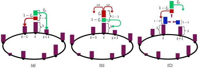
Figure 1: Schematic representation of the mass-chipping models MCM I, MCM II, and MCM III: (a) In MCM I, a site $i$ on a periodic lattice (shaped as a dark oval) having mass $m_{i}$ (dark violet), retains a fraction $\lambda$ of its mass (dark violet), while a random fraction $\xi_{i}$ of the chipped-off mass (green) migrates to the right neighbor, and the remaining fraction of the chipped mass(red) moves to the left side. (b) In MCM II, a random fraction $\xi_{i}$ of chipped-off mass(red) moves either left or nearest neighbor with equal probability, while the rest of the chipped mass(green) is deposited back to the same site $i$. (c) In MCM III, a fraction equivalent to $1-\lambda$ of the mass (blue) is chipped off from sites $i$ and $i+1$. This extracted mass is then recombined and subsequently redistributed in a way such that site $i$ receives a random fraction of $1-\xi_{i}$ (red), while site $i+1$ acquires a fraction of $\xi_{i}$ (green).

III Theory: MCM I

In this section, we study in detail the first variant of mass-chipping models, i.e., MCM I, on a periodic one-dimensional lattice of size $L$; For other models MCMs II and III, we later state the results, which can be derived following the techniques developed in this section.

A site $i$, with $i=0$, $1$, $\ldots$, $L-1$, possess a mass $m_{i}$, which can take continuous value in the interval $0\leq m_{i}\leq M$; total mass $M=\sum_{i=0}^{L-1}m_{i}=M$ remains conserved throughout and is the only conserved quantity. Density is defined as $\rho=M/L$, however we denote $\rho_{i}(t)=\langle m_{i}(t)\rangle$ as local density at site $i$ and at time $t$. Notably, unlike in MCMs II and III, a site in MCM I is stochastically updated in a way that simultaneously impacts its immediate neighbours, as stated in the previous section. This results in nonzero spatial correlations, making the calculations nontrivial.

We can now explicitly write down the stochastic update rules for mass $m_{i}(t)$ at site $i$ and at time $t$ during an infinitesimal time interval $(t,t+dt)$,

$$m_{i}(t+dt)=\begin{cases}\textbf{event}&\textbf{prob.}\\ m_{i}(t)-\tilde{\lambda}m_{i}(t)&dt\\ m_{i}(t)+\tilde{\lambda}\xi_{i-1}m_{i-1}(t)&dt\\ m_{i}(t)+\tilde{\lambda}\tilde{\xi}_{i+1}m_{i+1}(t)&dt\\ m_{i}(t)&(1-3dt),\end{cases}$$ (5)

where $\xi_{j}\in(0,1)$ is a random variable, which, for simplicity, is taken to be uniformly distributed; generalization of the results to other distributions is straightforward. Using the above dynamical update rules, the time-evolution of local mass can be written as

$$\frac{d}{dt}\left\langle m_{i}(t)\right\rangle=D(\lambda)\left(\left\langle m_{i-1}(t)\right\rangle-2\left\langle m_{i}(t)\right\rangle+\left\langle m_{i+1}(t)\right\rangle\right),$$ (6)

where $D(\lambda)=\tilde{\lambda}/2$ is the bulk-diffusion coefficient for MCM I. Note that $D$ is independent of density, leading to some important simplifications in the hierarchy for nass and current correlation functions, which, as we show later, actually close.

III.1 Definitions and notations

At this point, we introduce time-integrated bond current $\mathcal{Q}_{i}(t)$, which is the cumulative current across bond $(i,i+1)$ in the time interval time $(0,t)$. The time-integrated current across the $i^{th}$ bond during an infinitesimal time interval $[t,t+dt]$ is simply $\mathcal{J}_{i}(t)dt$, where instantaneous bond current

$$\mathcal{J}_{i}(t)\equiv\frac{d\mathcal{Q}_{i}(t)}{dt},$$ (7)

and therefore we have the time-integrated current across bond $(i,i+1)$

$$\mathcal{Q}_{i}(t)=\int\limits_{0}^{t}dt^{\prime}\mathcal{J}_{i}(t^{\prime}).$$ (8)

We can then express Eq.(6), the time evolution of the local density $\rho_{i}(t)=\langle m_{i}(t)\rangle$, in terms of a continuity equation for local density $\rho_{i}(t)=\langle m_{i}(t)\rangle$ and the average local current $\langle\mathcal{J}_{i}(t)\rangle$ simply as

$$\frac{d}{dt}\rho_{i}(t)=\langle\mathcal{J}_{i}(t)-\mathcal{J}_{i+1}(t)\rangle.$$ (9)

It is useful to decompose the instantaneous bond current as the sum of a diffusive component $\mathcal{J}_{i}^{(d)}(t)$ and a fluctuating component $\mathcal{J}_{i}^{(fl)}$ as

$$\mathcal{J}_{i}(t)=\mathcal{J}_{i}^{(d)}(t)+\mathcal{J}_{i}^{(fl)}(t),$$ (10)

where we can identify the diffusive current $\mathcal{J}_{i}^{(d)}(t)$ as

$$\mathcal{J}_{i}^{(d)}(t)\equiv D(\lambda)\big{[}m_{i}(t)-m_{i+1}(t)\big{]}.$$ (11)

The diffusion constant $D(\lambda)$ depends only on the chipping constant $\tilde{\lambda}$, not density $\rho$. It should be noted that the average fluctuating current $\langle\mathcal{J}_{i}^{(fl)}\rangle=0$, implying $\langle\mathcal{J}_{i}(t)\rangle=\langle\mathcal{J}_{i}^{(d)}(t)\rangle$. Indeed, one could interpret $\mathcal{J}_{i}^{(fl)}(t)$ as a fast varying “noise” current around the slowly varying diffusive (“hydrodynamic”) current component $\mathcal{J}_{i}^{(d)}(t)$. This decomposition of current is important because, as we show later explicitly, the fluctuation statistics of $\mathcal{J}_{i}^{(fl)}(t)$ is in fact strictly delta-correlated in time and short-ranged in space, whereas the diffusive current $\mathcal{J}_{i}^{(d)}(t)$ is long-ranged in time (in fact, a power law) and short-ranged in space.

For convenience, we introduce the following notation for correlation function $C_{r}^{AB}(t,t^{\prime})$ involving any two local observable $A_{i}(t)$ and $B_{j}(t^{\prime})$, with $t\geq t^{\prime}$,

$$C_{r=|j-i|}^{AB}(t,t^{\prime}) =\langle A_{i}(t)B_{j}(t^{\prime})\rangle-\langle A_{i}(t)\rangle\langle B_{j}(t^{\prime})\rangle$$ (12)

$$\equiv\langle A_{i}(t)B_{j}(t^{\prime})\rangle_{c},$$

where $r=|j-i|$ is the relative distance. We denote the spatial Fourier transform of the correlation function $C_{r}^{AB}(t,t^{\prime})$ as given below

$$\tilde{C}_{q}^{AB}(t,t^{\prime})=\sum\limits_{r=0}^{L-1}C_{r}^{AB}(t,t^{\prime})e^{iqr},$$ (13)

where $q=2\pi s/L$ and $s=0,1,\dots,L-1$; the inverse Fourier transform is given by

$$C_{r}^{AB}(t,t^{\prime})=\frac{1}{L}\sum\limits_{q}\tilde{C}_{q}^{AB}(t,t^{\prime})e^{-iqr}.$$ (14)

III.2 Calculation scheme

In this section we describe our calculation scheme in details for MCM I. The stochastic dynamical rules for time-integrated current $\mathcal{Q}_{i}(t)$ in an infinitesimal time interval $(t,t+dt)$ can be written as

$$\mathcal{Q}_{i}(t+dt)=\begin{cases}\textbf{event}&\textbf{prob.}\\ \mathcal{Q}_{i}(t)+\tilde{\lambda}\xi_{i}m_{i}(t)&dt\\ \mathcal{Q}_{i}(t)-\tilde{\lambda}\xi_{i+1}m_{i+1}(t)&dt\\ \mathcal{Q}_{i}(t)&(1-2dt).\end{cases}$$ (15)

The above update rules allow us to derive the time-evolution equation for the first moment of the time-integrated bond-current $\mathcal{Q}_{i}(t)$ as follows:

$$\frac{d\langle\mathcal{Q}_{i}(t)\rangle}{dt}=D\langle m_{i}(t)-m_{i+1}(t)\rangle=\langle\mathcal{J}_{i}^{(d)}(t)\rangle.$$ (16)

Using the update rule as in Eq.(15), the infinitesimal time-evolution equation for following product of the time-integrated currents at two different times $t$ and $t^{\prime}$($t>t^{\prime}$) can be written as

$$\mathcal{Q}_{i}(t+dt)\mathcal{Q}_{i+r}(t^{\prime})=~{}~{}~{}~{}~{}~{}~{}~{}~{}~{}~{}~{}~{}~{}~{}~{}~{}~{}~{}~{}~{}~{}~{}~{}~{}~{}~{}~{}~{}~{}$$

$$\begin{cases}\textbf{event}&\textbf{prob.}\\ [\mathcal{Q}_{i}(t)+\tilde{\lambda}\xi_{i}m_{i}(t)]\mathcal{Q}_{i+r}(t^{\prime})&dt\\ [\mathcal{Q}_{i}(t)-\tilde{\lambda}\xi_{i+1}m_{i+1}(t)]\mathcal{Q}_{i+r}(t^{\prime})&dt\\ \mathcal{Q}_{i}(t)\mathcal{Q}_{i+r}(t^{\prime})&(1-2dt).\end{cases}$$ (17)

Now expressing Eq.(19) in terms of mass and after some algebraic manipulation, we immediately get the following equality,

$$\frac{d}{dt}C_{r}^{\mathcal{Q}\mathcal{Q}}(t,t^{\prime})=C_{r}^{\mathcal{J}^{(d)}\mathcal{Q}}(t,t^{\prime}).$$ (18)

Interestingly, while calculating time derivative of current (or related observales), Eq. (18) can be simply obtained by using a convenient thumb rule where one takes the time derivative inside angular brackets as

$$\begin{aligned} \frac{d}{dt}\left\langle\mathcal{Q}_{i}(t)\mathcal{Q}_{i+r}(t^{\prime})\right\rangle_{c}&\equiv\left\langle\frac{d\mathcal{Q}_{i}(t)}{dt}\mathcal{Q}_{i+r}(t^{\prime})\right\rangle\\ &-\left\langle\frac{d\mathcal{Q}_{i}(t)}{dt}\right\rangle\left\langle\mathcal{Q}_{i+r}(t^{\prime})\right\rangle.\end{aligned}$$ (19)

Then by replacing the instantaneous current through the equivalence relation ${d\mathcal{Q}_{i}(t)}/{dt}\equiv D(m_{i}-m_{i+1})+\mathcal{J}_{i}^{(fl)}$ and subsequently dropping the noise correlation as $\langle{\cal J}_{i}^{(fl)}(t){\cal Q}_{i+r}(t^{\prime})\rangle=0$ for $t>t^{\prime}$, we get Eq. (18).

Now, using Eq. (11) into rhs of Eq.(18), we can immediately express the time evolution of unequal-space-time current-current correlation function in terms of the unequal-space-time mass-current correlation function,

$$\frac{d}{dt}C_{r}^{\mathcal{Q}\mathcal{Q}}(t,t^{\prime})=D\big{(}C_{r}^{m\mathcal{Q}}(t,t^{\prime})-C_{r-1}^{m\mathcal{Q}}(t,t^{\prime})\big{)}.$$ (20)

From the above equation, we see that we now rwquire to calculate the unequal-time mass-current correlation $C_{r}^{m\mathcal{Q}}(t,t^{\prime})$ in order to determine the unequal-time current-current correlation $C_{r}^{\mathcal{Q}\mathcal{Q}}(t,t^{\prime})$. The time evolution of the correlation function $C_{r}^{m\mathcal{Q}}(t,t^{\prime})$ can be obtained by using infinitesimal-time update rules for the following mass-current product at a later time $t+dt$ as

$$m_{i}(t+dt)Q_{i+r}(t^{\prime})=~{}~{}~{}~{}~{}~{}~{}~{}~{}~{}~{}~{}~{}~{}~{}~{}~{}~{}~{}~{}~{}~{}~{}~{}~{}~{}~{}~{}~{}~{}~{}~{}~{}~{}~{}~{}~{}~{}~{}~{}~{}~{}~{}~{}$$

$$\begin{cases}\textbf{event}&\textbf{prob.}\\ [m_{i}(t)-\tilde{\lambda}m_{i}(t)]Q_{i+r}(t^{\prime})&dt\\ [m_{i}(t)+\tilde{\lambda}\xi_{i-1}m_{i-1}(t)]Q_{i+r}(t^{\prime})&dt\\ [m_{i}(t)+\tilde{\lambda}\tilde{\xi}_{i+1}m_{i+1}(t)]Q_{i+r}(t^{\prime})&dt\\ m_{i}(t)Q_{i+r}(t^{\prime})&(1-3dt).\end{cases}$$ (21)

Using above update rule the time evaluation of unequal-time mass-current can be expressed in the following form,

$$\begin{aligned} &\frac{d}{dt}C_{r}^{m\mathcal{Q}}(t,t^{\prime})\\ &=D\langle(m_{i+1}(t)-2m_{i}(t)+m_{i-1}(t))\mathcal{Q}_{i+r}(t^{\prime})\rangle_{c}\\ &=D\sum\limits_{k}\Delta_{r,k}C_{k}^{m\mathcal{Q}}(t,t^{\prime}),\end{aligned}$$ (22)

where $\Delta_{r,k}=\delta_{r-1,k}-2\delta_{r,k}+\delta_{r+1,k}$ is the discrete Laplacian operator. Now, equations (20) and (22) can be expressed in terms of the Fourier modes as defined in Eq.(13),

$$\frac{d}{dt}\tilde{C}_{q}^{\mathcal{Q}\mathcal{Q}}(t,t^{\prime})=D\tilde{C}_{q}^{m\mathcal{Q}}(t,t^{\prime})\left(1-e^{iq}\right),$$ (23)

and

$$\frac{d}{dt}\tilde{C}_{q}^{m\mathcal{Q}}(t,t^{\prime})=-D\omega_{q}\tilde{C}_{q}^{m\mathcal{Q}}(t,t^{\prime}),$$ (24)

where the eigenvalue of discrete Laplacian is written as follows

$$\omega_{q}=2\left(1-\cos q\right).$$ (25)

Also, $\tilde{C}_{q}^{\mathcal{Q}\mathcal{Q}}(t,t^{\prime})$ and $\tilde{C}_{q}^{m\mathcal{Q}}(t,t^{\prime})$ are the Fourier transforms of the quantities $C_{r}^{\mathcal{Q}\mathcal{Q}}(t,t^{\prime})$ and $C_{r}^{m\mathcal{Q}}(t,t^{\prime})$, respectively. Now, Eq.(23) and Eq.(24), can be integrated to have

$$\tilde{C}_{q}^{\mathcal{Q}\mathcal{Q}}(t,t^{\prime}) =D\int\limits_{t^{\prime}}^{t}dt^{\prime\prime}\tilde{C}_{q}^{m\mathcal{Q}}(t^{\prime\prime},t^{\prime})\left(1-e^{iq}\right)$$ (26)

$$+\tilde{C}_{q}^{\mathcal{Q}\mathcal{Q}}(t^{\prime},t^{\prime}),$$

and

$$\tilde{C}_{q}^{m\mathcal{Q}}(t,t^{\prime})=e^{-D\omega_{q}(t-t^{\prime})}\tilde{C}_{q}^{m\mathcal{Q}}(t^{\prime},t^{\prime})$$ (27)

respectively. The equations Eq.(26) and Eq.(27) suggest that the dynamic correlation of current-current $C_{r}^{m\mathcal{Q}\mathcal{Q}}(t^{\prime},t^{\prime})$ and mass-current $C_{r}^{m\mathcal{Q}}(t^{\prime},t^{\prime})$ at equal time are required to obtain the respective dynamic correlation at unequal time, from their corresponding update rules.

The time-evolution equation for the equal-time current-current spatial correlation $C_{r}^{\mathcal{Q}\mathcal{Q}}(t,t)$ can be written from the infinitesimal update rules for the product of the following random variables,

$$\mathcal{Q}_{i}(t+dt)\mathcal{Q}_{i+r}(t+dt)=~{}~{}~{}~{}~{}~{}~{}~{}~{}~{}~{}~{}~{}~{}~{}~{}~{}~{}~{}~{}~{}~{}~{}~{}~{}~{}~{}~{}~{}~{}~{}~{}~{}~{}~{}~{}~{}~{}~{}~{}$$

$$\begin{cases}\textbf{event}&\textbf{prob.}\\ \mathcal{Q}_{i}\mathcal{Q}_{i+r}+\tilde{\lambda}\left(\xi_{i}m_{i}-\tilde{\xi}_{i+1}m_{i+1}\right)\mathcal{Q}_{r}\\ +\tilde{\lambda}\left(\xi_{r}m_{r}-\tilde{\xi}_{r+1}m_{r+1}\right)\mathcal{Q}_{i}&dt\\ \mathcal{Q}_{i}\mathcal{Q}_{i+r}+\tilde{\lambda}^{2}(\xi_{i}^{2}m_{i}^{2}+\tilde{\xi}_{i+1}^{2}m_{i+1}^{2})&\delta_{r,0}dt\\ \mathcal{Q}_{i}\mathcal{Q}_{i+r}-\tilde{\lambda}^{2}\xi_{i}\tilde{\xi}_{i}m_{i}^{2}&\delta_{r,1}dt\\ \mathcal{Q}_{i}\mathcal{Q}_{i+r}-\tilde{\lambda}^{2}\xi_{i+1}\tilde{\xi}_{i+1}m_{i+1}^{2}&\delta_{r,-1}dt\\ \mathcal{Q}_{i}\mathcal{Q}_{i+r}&1-\sum dt,\end{cases}$$ (28)

where $\sum=1+\delta_{r,0}+\delta_{r,1}+\delta_{r,-1}$ represents the total exit rate. Hence, from the above update rules, we can deduce the following time-evolution equation,

$$\frac{d}{dt}\left\langle\mathcal{Q}_{i}(t)\mathcal{Q}_{i+r}(t)\right\rangle_{c} =D\left\langle(m_{i}-m_{i+1})\mathcal{Q}_{r}\right\rangle_{c}$$ (29)

$$+D\left\langle\mathcal{Q}_{i}(m_{i+r}-m_{i+r+1})\right\rangle_{c}+\Gamma_{r},$$

where $\Gamma_{r}$ can be written in terms of steady-state single-site mass fluctuation (function of $\rho$),

$$\Gamma_{r}(\rho)=\frac{\tilde{\lambda}^{2}}{6}\langle m_{i}^{2}\rangle(4\delta_{r,0}-\delta_{r,1}-\delta_{r,-1}).$$ (30)

For convenience, we introduce the following quantity,

$$\chi(\rho)\equiv\frac{\tilde{\lambda}^{2}}{6}\langle m_{i}^{2}\rangle$$ (31)

which, as we show later, is nothing but the density-dependent transport coefficient, called mobility $\chi(\rho)=\lim\limits_{T\to\infty,L\to\infty}L\left\langle\mathcal{Q}_{i}^{2}(T)\right\rangle/2T$ - the scaled bond-current fluctuation, with infinite time limit $T\to\infty$ taken first [23]. As we shall demonstrate later, the mobility $\chi(\rho)$ can be exactly equated to another related transport coefficient, we call it “operational” mobility $\chi_{op}(\rho)$, which is ratio of the current (response) to a small externally applied biasing force (perturbation) [39]. The expression for the second moment of mass $\langle m_{i}^{2}\rangle$ in the steady state can be written in terms of chipping constant $\tilde{\lambda}$ and the density $\rho$ as given below [13],

$$\langle m_{i}^{2}\rangle=\frac{3\rho^{2}}{3-2\tilde{\lambda}}.$$ (32)

We can now substitute Eq.(31) into Eq.(30) to express $\Gamma_{r}$ in terms of the system’s mobility $\chi$ as

$$\Gamma_{r}(\rho)=4\chi(\rho)\delta_{r,0}-\chi(\delta_{r,1}+\delta_{r,-1}).$$ (33)

It is interesting to note that $\Gamma_{r}$ has a direct connection to the steady-state mass-mass correlation $C_{r}^{mm}$, through the relation

$$\Gamma_{r}=2DC_{r}^{mm},$$ (34)

which should be generic for diffusive systems [44, 45]. Later we show that the quantity $\Gamma_{r}$ is also related to the spatial correlation function for the fluctuating (“noise”) current, thus establishing a direct (presumably generic) connection between (noise) current fluctuation and density fluctuation in a diffusive system and, thus, characterizing the role of steady-state spatial structure in determining the large-scale dynamic properties. This is precisely how density and current fluctuations, as well as relaxation properties (through bulk-diffusivity), are intricately coupled to one another, resulting in an equilibrium-like Einstein relation, as demonstrated subsequently.

Now, by using the following formula

$$\begin{aligned} D\left\langle(m_{i}-m_{i+1})\mathcal{Q}_{r}\right\rangle_{c}=\frac{D}{L}\sum\limits_{q}(1-e^{iq})\tilde{C}_{q}^{m\mathcal{Q}}(t,t)e^{-iqr}\end{aligned}$$ (35)

in Eq.(29) and performing some algebraic manipulations, we obtain the following expression,

$$\frac{d}{dt}C_{r}^{\mathcal{Q}\mathcal{Q}}(t,t)=\frac{D}{L}\sum\limits_{q}(1-e^{iq})\tilde{C}_{q}^{m\mathcal{Q}}(t,t)(2-\omega_{qr})+\Gamma_{r},$$ (36)

where $\omega_{qr}=2\left(1-\cos(qr)\right)$, as indicated in Eq.(25). After integrating both sides of the above equation, we obtain the equal-time current-current dynamic correlation as follows:

$$C_{r}^{\mathcal{Q}\mathcal{Q}}(t,t)=\int\limits_{0}^{t}dt^{\prime}\Gamma_{r}(t^{\prime})+$$ (37)

$$\frac{D}{L}\int\limits_{0}^{t}dt^{\prime}\sum\limits_{q}\tilde{C}_{q}^{m\mathcal{Q}}(t^{\prime},t^{\prime})(1-e^{iq})(2-\omega_{qr}).$$

Now, to obtain the desired form of the above equal-time correlation for current, we calculate the equal-time correlation function $C_{r}^{m\mathcal{Q}}(t,t)$ by using the following infnitesimal-time update rule,

$$m_{i}(t+dt)\mathcal{Q}_{i+r}(t+dt)=~{}~{}~{}~{}~{}~{}~{}~{}~{}~{}~{}~{}~{}~{}~{}~{}~{}~{}~{}~{}~{}~{}~{}~{}~{}~{}~{}~{}~{}~{}~{}~{}~{}~{}~{}~{}$$

$$\begin{cases}\textbf{event}&\textbf{prob.}\\ m_{i}\mathcal{Q}_{i+r}+\tilde{\lambda}m_{i}(\xi_{i+r}m_{i+r}-\tilde{\xi}_{i+r+1}m_{i+r+1})\\ +\tilde{\lambda}\left(\tilde{\xi}_{i+1}m_{i+1}-m_{i}+\xi_{i-1}m_{i-1}\right)\mathcal{Q}_{r}&dt\\ m_{i}\mathcal{Q}_{i+r}-\tilde{\lambda}^{2}(\xi_{i}m_{i}^{2}+\tilde{\xi}_{i+1}^{2}m_{i+1}^{2})&\delta_{r,0}dt\\ m_{i}\mathcal{Q}_{i+r}+\tilde{\lambda}^{2}(\tilde{\xi}_{i}m_{i}^{2}+\xi_{i-1}^{2}m_{i-1}^{2})&\delta_{r,-1}dt\\ m_{i}\mathcal{Q}_{i+r}+\tilde{\lambda}^{2}\tilde{\xi}_{i+1}\xi_{i+1}m_{i+1}^{2}&\delta_{r,1}dt\\ m_{i}\mathcal{Q}_{i+r}-\tilde{\lambda}^{2}\xi_{i-1}\tilde{\xi}_{i-1}m_{i-1}^{2}&\delta_{r,-2}dt\\ m_{i}\mathcal{Q}_{i+r}&1-\sum dt,\end{cases}$$ (38)

where $\sum=1+\delta_{r,0}+\delta_{r,1}+\delta_{r,-1}+\delta_{r,-2}$ is the total exit rate. Using the above dynamical update rules, we obtain the following equation:

$$\frac{d}{dt}C_{r}^{m\mathcal{Q}}(t,t)=D\left(C_{r-1}^{m\mathcal{Q}}-2C_{r}^{m\mathcal{Q}}+C_{r+1}^{m\mathcal{Q}}\right)+A_{r},$$ (39)

where $A_{r}$ is given by

$$\begin{aligned} A_{r}&=\frac{\tilde{\lambda}}{2}\langle m_{i}m_{i+r}-m_{i}m_{i+r+1}\rangle_{c}\\ &-\frac{5\tilde{\lambda}^{2}}{6}\langle m_{i}^{2}\rangle\delta_{r,0}+\frac{\tilde{\lambda}^{2}}{6}\langle m_{i}^{2}\rangle\delta_{r,1}-\frac{\tilde{\lambda}^{2}}{6}\langle m_{i}^{2}\rangle\delta_{r,-2}.\end{aligned}$$ (40)

From the above equation, it is evident that $A_{r}$ can be represented in terms of the equal-time spatial correlation of masses, which can be calculated by using the following infinitesimal-time update rules, $m_{i}(t+dt)m_{i+r}(t+dt)=$

$$\begin{cases}\textbf{event}&\textbf{prob.}\\ \tilde{\lambda}\left(\tilde{\xi}_{i+1}m_{i+1}+\xi_{i-1}m_{i-1}\right)m_{r}\\ +\tilde{\lambda}m_{i}(\tilde{\xi}_{i+r+1}m_{i+r+1}+\xi_{i+r-1}m_{i+r-1})\\ (1-2\tilde{\lambda})m_{i}m_{i+r}&dt\\ m_{i}m_{i+r}+\tilde{\lambda}^{2}(m_{i}^{2}+\tilde{\xi}_{i+1}^{2}m_{i+1}^{2}+m_{i-1}^{2}\xi_{i-1}^{2})&\delta_{r,0}dt\\ m_{i}m_{i+r}-\tilde{\lambda}^{2}(\tilde{\xi}_{i+1}m_{i+1}^{2}+\xi_{i}m_{i}^{2})&\delta_{r,1}dt\\ m_{i}m_{i+r}+\tilde{\lambda}^{2}(\tilde{\xi}_{i}m_{i}^{2}+\xi_{i-1}m_{i-1}^{2}&\delta_{r,-1}dt\\ m_{i}m_{i+r}-\tilde{\lambda}^{2}\xi_{i+1}\tilde{\xi}_{i+1}m_{i+11}^{2}&\delta_{r,2}dt\\ m_{i}m_{i+r}-\tilde{\lambda}^{2}\xi_{i-1}\tilde{\xi}_{i-1}m_{i-1}^{2}&\delta_{r,-2}dt\\ m_{i}m_{i+r}&1-\sum dt,\end{cases}$$ (41)

where $\sum=1+\delta_{r,0}+\delta_{r,1}+\delta_{r,-1}+\delta_{r,-2}+\delta_{r,2}$ is the total exit rate. Using the above dynamical update rules we obtain the following equation:

$$\frac{d}{dt}C_{r}^{mm}(t,t)=2D\sum\limits_{k}\left\langle m_{0}\Delta_{r,k}m_{k}\right\rangle_{c}+B_{r},$$ (42)

where the source term $B_{r}$ can be expressed in terms of the second moment of a single site mass as,

$$\begin{aligned} B_{r}=\frac{\tilde{\lambda}^{2}\left\langle m_{i}^{2}\right\rangle}{6}[10\delta_{r,0}-6(\delta_{r,1}+\delta_{r,-1})+(\delta_{r,2}+\delta_{r,-2})].\end{aligned}$$ (43)

Then using the steady-state condition $dC_{r}^{mm}(t,t)/dt=0$, we obtain:

$$2D\left[C_{r+1}^{mm}-2C_{r}^{mm}+C_{r-1}^{mm}\right]+B_{r}=0.$$ (44)

Now, Eq.(44) can be exactly solved by employing a generating function method (which is slightly different than that used in [13]),

$$G(z)=\sum\limits_{r=0}^{\infty}C_{r}^{mm}z^{r};$$ (45)

we present it here for completeness of the various calculations and derivations of a set of fluctuation relations, which will follow in the subsequent sections. By multiplying both sides of Eq.(44) by $z^{r}$ and then summing over $r$, we can express the equation in terms of $G(z)$ as follows:

$$G(z)=\frac{C_{0}^{mm}[6-(10-6z+z^{2})\tilde{\lambda}]-6zC_{1}^{mm}-(10-6z+z^{2})\rho^{2}}{6(1-z)^{2}},$$

where we use identities, $\sum_{r=0}^{\infty}C_{r+1}^{mm}z^{r}=[G(z)-C_{0}^{mm}]/z$, $\sum_{r=0}^{\infty}C_{r-1}^{mm}z^{r}=C_{1}^{mm}+zG(z)$, and $\left\langle m_{i}^{2}\right\rangle=C_{0}^{mm}+\rho^{2}$. From the equation above, it is evident that $G(z)$ has a second-order pole singularity at $z=1$. However, considering that $G(z=1)$ represents the sum of density correlations and thus should be finite, implying that $\lim_{z\to 1}G(z)$ must also be finite. Therefore the numerator, and its derivative, must also vanish as $z\to 1$. From this root-cancellation conditions, we get the following two equations,

$$C_{0}^{mm}(6-5\tilde{\lambda})-6C_{1}^{mm}-5\rho^{2}=0,$$ (46)

and

$$2\tilde{\lambda}C_{0}^{mm}+3C_{1}^{mm}-2\rho^{2}=0.$$ (47)

By solving the above equations, we finally obtain the desired solution for the generating function,

$$G(z)=\frac{2\tilde{\lambda}\rho^{2}}{3-2\tilde{\lambda}}-\frac{\tilde{\lambda}\rho^{2}}{2(3-2\tilde{\lambda})}z,$$ (48)

which immediately leads to the explicit analytical expression for the steady-state spatial correlation function $C_{r}^{mm}$ for mass,

$$C_{r}^{mm}=\langle m_{i}m_{i+r}\rangle-\rho^{2}=\begin{cases}\frac{2\tilde{\lambda}\rho^{2}}{3-2\tilde{\lambda}}&\text{for}~{}r=0\\ -\frac{\tilde{\lambda}\rho^{2}}{2(3-2\tilde{\lambda})}&\text{for}~{}|r|=1\\ 0&\text{otherwise}.\end{cases}$$ (49)

Note that the above correlation function was previously calculated through a different method in Ref. [13]. Now the steady-state spatial correlation function for mass can be readily expressed in terms of the particle mobility $\chi$,

$$C_{r}^{mm}=\frac{\chi}{\tilde{\lambda}}(4\delta_{r,0}-\delta_{r,1}-\delta_{r,-1}).$$ (50)

Now, by summing both sides of Eq.(50) over $r$, we obtain a fluctuation relation between mass fluctuation and the mobility (equivalently, the current fluctuation),

$$\sum\limits_{r=-\infty}^{\infty}C_{r}^{mm}=\frac{2\chi}{\tilde{\lambda}}.$$ (51)

Now, in the steady state, we write $A_{r}$ by simply using Eq.(50) in Eq.(40),

$$A_{r}=-\frac{5}{2}\chi(\delta_{r,0}-\delta_{r,-1})+\frac{1}{2}\chi(\delta_{r,1}-\delta_{r,-2}).$$ (52)

We now express Eq. (39) in the Fourier space as

$$\frac{d}{dt}\tilde{C}_{q}^{m\mathcal{Q}}(t,t)=-D\omega_{q}\tilde{C}_{q}^{m\mathcal{Q}}(t,t)+\tilde{f}_{q}(t),$$ (53)

where the Fourier transform of the source term $A_{r}$ is expressed as $\tilde{f}_{q}(t^{\prime})$ in the following equation:

$$\tilde{f}_{q}=-\chi(1-e^{-iq})\left(1+\frac{1}{2}\omega_{q}\right).$$ (54)

Equation (53) can now be integrated directly to obtain the following equation,

$$\tilde{C}_{q}^{m\mathcal{Q}}(t^{\prime},t^{\prime})=\int\limits_{0}^{t^{\prime}}dt^{\prime\prime}e^{-D\omega_{q}(t^{\prime}-t^{\prime\prime})}\tilde{f}_{q}(t^{\prime\prime}).$$ (55)

The above equation describes the equal-time dynamic correlation of mass-current, which appears in Eq.(37) and Eq.(27), making it necessary for the calculation of the equal-time current-current correlation and unequal-time mass-current, respectively. By substituting Eq.(55) into Eq.(27), leading to the following expression,

$$\tilde{C}_{q}^{m\mathcal{Q}}(t,t^{\prime})=\int\limits_{0}^{t^{\prime}}dt^{\prime\prime}e^{-D\omega_{q}(t-t^{\prime\prime})}\tilde{f}_{q}(t^{\prime\prime}).$$ (56)

III.3 Time-integrated current fluctuation

In this section, we apply the theoretical framework established in the previous section to finally compute the time-integrated bond-current fluctuation for MCM I. To achieve this, we insert Eq. (55) into Eq. (37), yielding an explicit expression for the time-integrated bond-current fluctuation at equal times, as follows:

$$C_{r}^{\mathcal{Q}\mathcal{Q}}(t,t)=\int\limits_{0}^{t}dt^{\prime}\Gamma_{r}(t^{\prime})+$$ (57)

$$\frac{D}{L}\sum\limits_{q}\int\limits_{0}^{t}dt^{\prime}\int\limits_{0}^{t^{\prime}}dt^{\prime\prime}e^{-D\omega_{q}(t^{\prime}-t^{\prime\prime})}\tilde{f}_{q}(t^{\prime\prime})(1-e^{iq})[2-\omega_{qr}].$$

Furthermore, by plugging in the equal-time current-current dynamic correlation $C_{r}^{\mathcal{Q}\mathcal{Q}}(t,t)$ from Eq.(57) and the unequal-time mass-current $\tilde{C}_{q}^{m\mathcal{Q}}(t,t^{\prime})$ from Eq.(56) into Eq.(26), we can obtain the final expression for the current-current dynamic correlation at unequal time:

$$C^{\mathcal{Q}\mathcal{Q}}_{r}(t,t^{\prime})= t^{\prime}\Gamma_{r}-\frac{\chi D}{L}\sum\limits_{q}\int\limits_{0}^{t^{\prime}}\differential{t^{\prime\prime}}\int\limits_{0}^{t^{\prime\prime}}\differential{t^{\prime\prime\prime}}e^{-D\omega_{q}(t^{\prime\prime}-t^{\prime\prime\prime})}\omega_{q}(1+\frac{1}{2}\omega_{q})(2-\omega_{qr})$$ (58)

$$-\frac{\chi D}{L}\sum\limits_{q}\int\limits_{t^{\prime}}^{t}\differential{t^{\prime\prime}}\int\limits_{0}^{t^{\prime}}\differential{t^{\prime\prime\prime}}e^{-D\omega_{q}(t^{\prime\prime}-t^{\prime\prime\prime})}\omega_{q}(1+\frac{1}{2}\omega_{q})e^{-iqr}.$$

We obtain the time-integrated bond-current fluctuation $\langle\mathcal{Q}^{2}(T)\rangle\equiv\langle\mathcal{Q}_{i}^{2}(T)\rangle=C_{0}^{\mathcal{Q}\mathcal{Q}}(T,T)$ from Eq.(58), by putting $t^{\prime}=t=T$ and $r=0$,

$$\langle\mathcal{Q}^{2}(T)\rangle=\frac{2\chi T}{L}+\frac{2\chi}{L}\sum\limits_{n=1}^{L-1}\left(1+\frac{\omega_{n}}{2}\right)\frac{(1-e^{-D\omega_{n}T})}{D\omega_{n}},$$ (59)

where $\omega_{n}=2(1-\cos(2\pi n/L))$, with $n=0,1,\cdots,L-1$. If we take the $T\to\infty$ limit first (i.e., $T\gg L^{2}$), we immediately obtain

$$\langle\mathcal{Q}^{2}(T)\rangle\simeq\frac{2\chi T}{L}+\frac{\chi}{D}\left(\frac{L}{6}-\frac{1}{L}\right)=\frac{2\chi T}{L}\left[1+{\cal O}\left(\frac{L^{2}}{DT}\right)\right].$$ (60)

In Eq. (59), we have identified two distinct time regimes that correspond to two the following cases.

Case 1: $DT\ll 1$

In the limit $DT\ll 1$, the system does not have sufficient time for building up of spatial correlations at neighboring sites, resulting in the bond-current fluctuation having no information of the spatial structure. In equation (59), we expand the exponential up to linear order for $DT\ll 1$ and obtain

$$\langle\mathcal{Q}^{2}(T)\rangle=\frac{2\chi T}{L}+\frac{2\chi}{L}\sum\limits_{n=1}^{L-1}\left(1+\frac{\omega_{n}}{2}\right)T.$$ (61)

To further simplify the above equation, we utilize the identity $\sum_{n=1}^{L-1}\omega_{n}=2L$, resulting in

$$\langle\mathcal{Q}^{2}(T)\rangle=\Gamma_{0}T=4\chi T.$$ (62)

where $\Gamma_{0}$ is the strength of fluctuating current as mentioned in Eq.(33) and shown exactly later.

In Figure [2], we present the simulation data for the time-integrated bond-current fluctuation, $\langle\mathcal{Q}^{2}(T)\rangle$, as a function of time $T$. The plot reveals three distinct growth behaviors of $\langle\mathcal{Q}^{2}(T)\rangle$ over time: $T$, $T^{1/2}$, and again $T$. We have examined the effects of varying chipping parameters on two different system sizes, namely $L=500$ and $L=1000$, with values of $\lambda$ set at 0.25 and 0.90. Additionally, we have included two plots that overlap in the $DT\ll 1$ region for the two system sizes with the same $\lambda$ values.

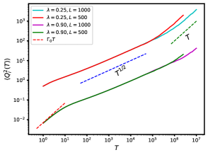
Figure 2: The time-integrated bond-current fluctuation, $\langle\mathcal{Q}_{i}^{2}(T)\rangle$, plotted as a function of time $T$ for various chipping parameter and system sizes. The cyan ($\lambda=0.25$, $L=1000$), magenta ($\lambda=0.90$, $L=1000$), red ($\lambda=0.25$, $L=500$), and green ($\lambda=0.90$, $L=500$) lines lines represent simulation data for global density $\rho=1$. The red dashed line represents the behavior $\Gamma_{0}T$ for $\lambda=0.90$ as mentioned in Eq.(62), while the blue and green dashed lines represent sub-diffusive $\sim T^{1/2}$ and diffusive $\sim T$ growth, respectively, as mentioned in Eq.(71).

Case 2: $DT\gg 1$

In the time limit $DT\gg 1$, the spatial correlations buid up in the systems. Interestingly Eq.(60) suggests that, in the large-time limit, $\langle Q_{i}^{2}\rangle$ asymptotically approaches $2\chi T/L$, indicating that, in the long-time regime, only three relevant parameters are required to characterize the diffusive system: $D$, $\chi$, and $L$. Moreover, it becomes evident that $\langle\mathcal{Q}_{i}^{2}\rangle$ and $T$ are related through a particular scaling combination, as given in Eq.(63). To further analyze the behavior, we introduce a scaled time-integrated bond-current fluctuation as follows:

$$\mathcal{W}\left(\frac{DT}{L^{2}}\right)\equiv\frac{D\langle\mathcal{Q}^{2}(T)\rangle}{2\chi L}$$ (63)

$$=\lim\limits_{L\to\infty}\frac{DT}{L^{2}}+\lim\limits_{L\to\infty}\frac{1}{L^{2}}\sum\limits_{q}\left(1+\frac{\omega_{q}}{2}\right)\frac{1-e^{-\omega_{q}DT}}{\omega_{q}},$$

or, equivalently, we can write the scaling function as

$$\mathcal{W}(y)=\lim\limits_{L\to\infty}\left[y+\frac{1}{L^{2}}\sum\limits_{q}\left(1+\frac{\omega_{q}}{2}\right)\frac{1-e^{-\omega_{q}L^{2}y}}{\omega_{q}}\right],~{}~{}$$ (64)

$$=\lim\limits_{L\to\infty}\left[y+\frac{1}{L^{2}}\sum\limits_{q}\frac{1-e^{-\omega_{q}L^{2}y}}{\omega_{q}}\right]+o\left(\frac{1}{L}\right),~{}~{}$$ (65)

where $\omega_{q}=2(1-\cos q)$, with $q=2\pi n/L$ and $n=1,2,\cdots,L-1$. In the expression of Eq. 64, the scaling function $\mathcal{W}(y)$ can be approximately written as the following integral representation,

$$\begin{aligned} \mathcal{W}(y)\simeq y+&\lim\limits_{L\to\infty}\frac{1}{\pi L}\int\limits_{\frac{2\pi}{L}}^{\pi}dq\frac{\left(1-e^{-L^{2}y\omega(q)}\right)}{\omega(q)}\\ &+\lim\limits_{L\to\infty}\frac{1}{2\pi L}\int\limits_{\frac{2\pi}{L}}^{\pi}dq\left(1-e^{-L^{2}y\omega(q)}\right).\\ \end{aligned}$$ (66)

By using variable transformation $z=\omega(q)L^{2}$ to Eq.(66) and taking the infinite system-size limit $L\to\infty$, we obtain the following expression,

$$\mathcal{W}(y)\simeq y+\frac{1}{2\pi}\int\limits_{4\pi^{2}}^{\infty}dz\frac{\left(1-e^{-zy}\right)}{z^{\frac{3}{2}}},$$ (67)

where we have used that the third term in the rhs of eq. (66) gives a subleading $o(1/L)$ contribution, which vanishes in the scaling limit. After performing the integration, we finally write

$$\mathcal{W}(y)\simeq y+\sqrt{\frac{y}{\pi}}\text{erfc}(2\pi\sqrt{y})+\frac{1-e^{-4\pi^{2}y}}{4\pi^{2}},$$ (68)

where $\text{erfc}(z)=1-\text{erf}(z)$, with error function,

$$\text{erf}(z)=\frac{2}{\sqrt{\pi}}\int\limits_{0}^{z}e^{-t^{2}}dt.$$ (69)

From Eq.(68), we can calculate the asymptotic forms of $\mathcal{W}(y)$ in two different limits,

$$\mathcal{W}(y)\simeq\begin{cases}\sqrt{\frac{y}{\pi}}&\text{for}~{}y\ll 1\\ y&\text{for}~{}y\gg 1.\end{cases}$$ (70)

In Fig.3, we illustrate the scaled time-integrated bond-current fluctuation $\langle\mathcal{Q}_{i}^{2}(T)\rangle D/(2\chi L)$ as a function of scaled time $DT/L^{2}$ for different chipping parameters and system sizes at a global density of $\rho=1$. The colored lines are obtained from simulations, and the black solid line corresponds to the theoretical lines as in Eq.(65). Two guiding dashed lines, which represent sub-diffusive behavior as $\sim y^{1/2}$ (blue) at early times, followed by diffusive growth as $\sim y$ (green) at longer times, as mentioned in Eq.(70).

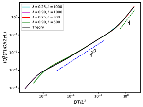
Figure 3: Scaled time-integrated bond-current fluctuation, $\langle\mathcal{Q}_{i}^{2}(T)\rangle D/(2\chi L)$, plotted against scaled time $DT/L^{2}$ for different chipping parameters and system sizes at a global density of $\rho=1$. The cyan ($\lambda=0.25$, $L=1000$), magenta ($\lambda=0.90$, $L=1000$), red ($\lambda=0.25$, $L=500$), and green ($\lambda=0.90$, $L=500$) lines lines represent simulation data. The two guiding dashed lines depict sub-diffusive behavior as $\sim y^{1/2}$ (blue) at early times, followed by a diffusive growth as $\sim y$ (green) at longer times. These trends are based on the scaling function $\mathcal{W}(y)$ [as in Eq.(70)]. The black solid line corresponds to theoretical results [as in Eq.(65)] and demonstrates excellent agreement with the simulations.

Now combining all the temporal regimes discussed abose, we can summarize asymptotic behaviors of the time-integrated bond-current $\langle\mathcal{Q}^{2}(T)\rangle$ in the following three regimes:

$$\langle\mathcal{Q}^{2}(T)\rangle=\begin{cases}4\chi T&\text{for}~{}DT\ll 1\\ \frac{2\chi}{\sqrt{D\pi}}T^{\frac{1}{2}}&\text{for}~{}1\ll DT\ll L^{2}\\ \frac{2\chi T}{L}&\text{for}~{}DT\gg L^{2}.\end{cases}$$ (71)

III.3.1 Space-time integrated current

In this section, we will focus on the calculation of the steady-state variance $\langle\mathcal{Q}_{sub}^{2}(l,T)\rangle-\langle\mathcal{Q}_{sub}(l,T)\rangle^{2}=\langle\mathcal{Q}_{sub}^{2}(l,T)\rangle$ of the cumulative (space-time integrated) actual particle current $\mathcal{Q}_{sub}(l,T)=\sum_{i=0}^{l-1}\mathcal{Q}_{i}(T)$ across a subsystem of size $l$ and up to time $T$. The variance $\langle\mathcal{Q}_{sub}^{2}(l,T)\rangle$ can be expressed as follows:

$$\langle\mathcal{Q}_{sub}^{2}(l,T)\rangle=\left\langle\sum\limits_{i=1}^{l-1}\mathcal{Q}_{i}(T)\sum\limits_{j=1}^{l-1}\mathcal{Q}_{j}(T)\right\rangle.$$ (72)

The sum on the right-hand side of the equation can be simplified and expressed in terms of the current-current dynamic correlation at equal times:

$$\langle\mathcal{Q}_{sub}^{2}(l,T)\rangle=lC_{0}^{\mathcal{Q}\mathcal{Q}}(T,T)+\sum\limits_{r=1}^{l-1}2(l-r)C_{r}^{\mathcal{Q}\mathcal{Q}}(T,T).$$ (73)

Now, we can utilize Eq.(57) in the above equation and employ the following identity:

$$\sum\limits_{r=1}^{l-1}2(l-r)(2-\omega_{rq})=2\left(\frac{\omega_{lq}-l\omega_{q}}{\omega_{q}}\right).$$ (74)

Afterwards, we perform some algebraic manipulations, yielding the following expression:

$$\langle\mathcal{Q}_{sub}^{2}(l,T)\rangle =2\chi lT+2\chi T(1-\delta_{l,L})-\frac{2\chi D}{L}$$ (75)

$$\times\sum\limits_{q}\frac{(D\omega_{q}T-1+e^{-\omega_{q}DT})}{(\omega_{q}D)^{2}}\big{(}1+\frac{1}{2}\omega_{q}\big{)}\omega_{ql}.$$

Here, $\omega_{q}=2(1-\cos q)$, where $q=2\pi n/L$ and $n=1,2,\cdots,L-1$. The influence of the subsystem size $l$ comes into play through the Fourier mode $\omega_{ql}$ alone. We will now derive the asymptotic dependence of Eq.(75) on the subsystem size $l$ and time $T$, first by considering the limit $T\gg 1$ followed by $l\gg 1$, and then by reversing the order of the limits, i.e., $l\gg 1$ followed by $T\gg 1$.

Case 1: $T\gg 1$ and $l\gg 1$

When we first consider the limit $T\gg 1$ followed by $l\gg 1$, the above Eq.(75) simplifies to:

$$\langle\mathcal{Q}_{sub}^{2}(l,T)\rangle$$ (76)

$$\simeq\frac{2\chi l^{2}T}{L}+\frac{2\chi D}{L}\sum\limits_{q}\frac{(1-e^{-D\omega_{q}T})}{D^{2}\omega_{q}^{2}}\left(1+\frac{\omega_{q}}{2}\right)\omega_{ql}.$$

In the limit as $L\to\infty$, the sum in the above equation can be approximated to an integral form as follows:

$$\langle\mathcal{Q}_{sub}^{2}(l,T)\rangle$$ (77)

$$\simeq\frac{2\chi D}{\pi}\int\limits_{0}^{\pi}dq\frac{(1-e^{-D\omega(q)T})}{D^{2}\omega(q)^{2}}\left(1+\frac{\omega(q)}{2}\right)\omega(ql).$$ (78)

By using the approximation $\omega(lq)\simeq l^{2}q^{2}$ for a finite subsystem size $l$, and introducing a variable transformation $z=DTq^{2}$, we obtain

$$\langle\mathcal{Q}_{sub}^{2}(l,T)\rangle\simeq\frac{\chi l^{2}\sqrt{T}}{\pi\sqrt{D}}\int\limits_{0}^{\infty}dz(1-e^{-z})z^{-3/2}.$$ (79)

After evaluating the integral $\int_{0}^{\infty}dz(1-e^{-z})z^{-3/2}=2\sqrt{\pi}$, we obtain:

$$\frac{\langle\mathcal{Q}_{sub}^{2}(l,T)\rangle}{lT}\simeq\frac{2\chi}{\sqrt{\pi D}}\frac{l}{\sqrt{T}}.$$ (80)

Case 2: $l\gg 1$ and $T\gg 1$

In this specific order of taking the limit ($l\gg 1$ first and then $T\gg 1$), we make the approximation $\omega(ql)\simeq 2$, and the equation (75) can be expressed in integral form as:

$$\begin{aligned} &\frac{\langle\mathcal{Q}_{sub}^{2}(l,T)\rangle}{lT}\\ &\simeq 2\chi+\frac{2\chi}{l}+\frac{4\chi D}{lT\pi}\int\limits_{0}^{\pi}dq\frac{[D\omega(q)T-1+e^{-\omega(q)DT}]}{D^{2}\omega(q)^{2}}.\end{aligned}$$ (81)

Again using the variable transformation $z=DTq^{2}$, we obtain,

$$\begin{aligned} &\frac{\langle\mathcal{Q}_{sub}^{2}(l,T)\rangle}{lT}\\ &\simeq 2\chi+\frac{2\chi}{l}-\frac{2\chi\sqrt{DT}}{\pi l}\int\limits_{0}^{\infty}dz(z-1+e^{-z})z^{-\frac{5}{2}}.\end{aligned}$$ (82)

By employing the integral $\int_{0}^{\infty}dz(z-1+e^{-z})z^{-5/2}=4\sqrt{\pi}/3$ in the above equation, we can express the leading-order contribution as:

$$\frac{\langle\mathcal{Q}_{sub}^{2}(l,T)\rangle}{lT}\simeq 2\chi-\frac{8\chi}{3}\frac{\sqrt{D}}{\pi}\frac{\sqrt{T}}{l}$$ (83)

Hence, the asymptotic expression for the variance of the cumulative subsystem current, as presented in equation (75), is conditional on the order of limits for the two variables $T\gg 1$ and $l\gg 1$, i.e.,

$$\frac{\langle\mathcal{Q}_{sub}^{2}(l,T)\rangle}{lT}\simeq\begin{cases}\frac{2\chi}{\sqrt{\pi D}}\frac{l}{\sqrt{T}}~{}&\text{for}~{}T\gg 1,l\gg 1,\\ 2\chi-\frac{8\chi}{3}\frac{\sqrt{D}}{\pi}\frac{\sqrt{T}}{l}~{}&\text{for}~{}l\gg 1,T\gg 1.\end{cases}$$ (84)

The first expression in the equation above results from taking the limits in the following sequence: first $T\gg 1$ and then $l\gg 1$. In this specific order of limits, the scaled function $\langle\mathcal{Q}_{sub}^{2}(l,T)\rangle/lT$ decreases as $1/\sqrt{T}$ and eventually diminishes as $T$ approaches infinity. Conversely, if we reverse the order of limits, starting with $l\gg 1$ and then considering $T\gg 1$, we derive the second asymptotic expression found in Eq.(84). In essence, when $l\to\infty$, the scaled fluctuation of the subsystem current $\langle\mathcal{Q}_{sub}^{2}(l,T)\rangle/lT$ approaches $2\chi$ as $T$ increases,

$$\sigma_{\mathcal{Q}}^{2}\equiv\lim\limits_{l\to\infty}\lim\limits_{T\to\infty}\frac{\langle\mathcal{Q}_{sub}^{2}(l,T)\rangle}{lT}=\sum\limits_{r}\Gamma_{r}.$$ (85)

In the infinite subsystem limit, taken first, followed by the infinite-time limit, Eq. (85) can be viewed as a non-equilibrium version of the Green-Kubo relation, well-known in equilibrium systems. Interestingly, when we consider $l=L\gg 1$, which corresponds to the bond current summed over the entire system, we obtain the following identity:

$$\lim_{L\to\infty}\frac{\langle\mathcal{Q}_{sub}^{2}(L,T)\rangle}{LT}=2\chi=\sum_{r}\Gamma_{r}.$$ (86)

It is important to note that the above expression is valid for any finite time $T$. This is due to the fact that the diffusive part of the total current vanishes over the full system size, i.e., $\sum_{i=1}^{L}\mathcal{J}^{(d)}_{i}=0$, by definition. As a result, we are left with only the strength of the fluctuating part of the current, which leads to $\sum_{r}\Gamma_{r}=2\chi$.

Figure 4: The scaled space-time-integrated bond-current fluctuation, $\langle\mathcal{Q}_{sub}^{2}(l,T)\rangle$, is displayed as a function of time $T$ for various sub-system sizes: $l=100$ (lower blue solid line), $500$ (middle orange solid line), and $1000$ (top solid green line). The chosen chipping parameter for the model is $\lambda=0.25$ (fixed), with a system size of $L=1000$ and a global density of $\rho=1$. The black dashed line in the plot corresponds to the theoretical prediction derived from Eq.(75), and it precisely aligns with the respectable simulation data. Moreover, when the subsystem size equals the full system size, i.e., $l=L$, $\langle\mathcal{Q}_{sub}^{2}(L,T)\rangle/LT$ follows the behavior of $2\chi$ (magenta dashed lines), as indicated by Eq.(86).

In Figure 4, we plot the scaled subsystem current fluctuation $\langle\mathcal{Q}_{sub}^{2}(l,T)\rangle/lT$ against time $T$ for various subsystem sizes: $l=100$ (blue line), $l=500$ (orange line), and $l=L=1000$ (green line). The black dashed lines represent theoretical predictions that closely match the simulation data. A magenta dotted line at $2\chi$ overlays the data when $l=L$, indicating a limit where $l\to\infty$ is taken first. Notably, for smaller subsystem sizes, $\langle\mathcal{Q}_{sub}^{2}(l,T)\rangle/lT$ tends to zero as $T\to\infty$ limit taken first.

III.4 Instantaneous bond-current fluctuations

In this section, we calculate the spatio-temporal correlation of the instantaneous current, $C^{\mathcal{J}\mathcal{J}}_{r}(t)=\langle\mathcal{J}_{i}(t)\mathcal{J}_{r+r}(0)\rangle_{c}$, from the correlation of the time-integrated bond current and show that the instantaneous bond current is negatively correlated in time. This is accomplished by taking a double derivative of the time-integrated bond current correlation, which is expressed as follows:

$$C_{r}^{\mathcal{J}\mathcal{J}}(t,t^{\prime})=\left[\frac{d}{dt}\frac{d}{dt^{\prime}}C_{r}^{\mathcal{Q}\mathcal{Q}}(t,t^{\prime})\right],$$ (87)

Here, with the condition that $t\geq t^{\prime}$, we proceed to differentiate Eq.(58) twice, resulting in its rewritten form:

$$\begin{aligned} C_{r}^{\mathcal{J}\mathcal{J}}(t,t^{\prime})&=\Gamma_{r}\delta(t-t^{\prime})\\ &-\frac{\chi D}{L}\sum\limits_{q}e^{-D\omega_{q}(t-t^{\prime})}\omega_{q}\left(1+\frac{\omega_{q}}{2}\right)e^{-iqr}.\end{aligned}$$ (88)

To investigate the temporal behavior of instantaneous bond current, we set $r=0$ and $t>t^{\prime}=0$ in Eq.(88), and simplify the resulting equation into the following integral form by taking limit $L\to\infty$ as

$$C_{0}^{\mathcal{J}\mathcal{J}}(t,0)\simeq\frac{\chi D}{\pi}\int\limits_{0}^{\pi}dqe^{-D\omega(q)t}\omega(q)\left[1+\frac{\omega(q)}{2}\right],$$ (89)

where $\omega(q)=2(1-\cos q)$. Now, we approximate $\omega(q)\simeq q^{2}$ and make a variable transformation $z=Dq^{2}t$ to rewrite the above equation as follows:

$$C_{0}^{\mathcal{J}\mathcal{J}}(t,0)\simeq-\frac{\chi t^{-\frac{3}{2}}}{2\pi\sqrt{D}}\int\limits_{0}^{\infty}z^{\frac{1}{2}}e^{-z}dz,$$ (90)

where we have ignored the subleading term $O(t^{-5/2})$. We note that the sign is negative in Eq.(90). Finally, using the integral $\int_{0}^{\infty}z^{1/2}e^{-z}dz=\sqrt{\pi}/2$, the asymptotic form of the time-dependent instantaneous current for any time $t$ in the thermodynamic limit can be written as:

$$C_{0}^{\mathcal{J}\mathcal{J}}(t,0)\simeq\Gamma_{0}\delta(t)-\frac{\chi}{4\sqrt{\pi D}}t^{-\frac{3}{2}}.$$ (91)

Notably, the negative part of the above equation exhibits long-range behavior in the temporal domain, primarily due to the contribution of dynamic correlation from the diffusive current, i.e., $C_{0}^{\mathcal{J}^{(d)}\mathcal{J}^{(d)}}(t,0)\sim t^{-3/2}$. In contrast, the fluctuating current is short-ranged, given by $C_{r}^{\mathcal{J}^{(fl)}\mathcal{J}^{(fl)}}(t,0)=\delta(t)\Gamma_{r}$, where $\Gamma_{r}$ represents the strength of the fluctuating current.

Now, to check the spatial behavior of instantaneous current, we calculated this correlation at the same time, $t=t^{\prime}$. In that case Eq.(88) can be expressed as:

$$\begin{aligned} C_{r}^{\mathcal{J}\mathcal{J}}(t,t)=\Gamma_{r}\delta(0)-\frac{\chi D}{L}\sum\limits_{q}\omega_{q}\left(1+\frac{\omega_{q}}{2}\right)e^{-iqr}.\end{aligned}$$ (92)

After some algebraic manipulation of the above equation, it can be expressed in terms of the steady-state $(t\to\infty)$ density correlation $C_{r}^{mm}$ as follows:

$$\begin{aligned} C_{r}^{\mathcal{J}\mathcal{J}}&=\Gamma_{r}\delta(0)-D^{2}[3C_{r}^{mm}-(C_{r-1}^{mm}+C_{r+1}^{mm})].\end{aligned}$$ (93)

In Eq.(93), we can see that the spatial length scale of the instantaneous current is intimately tied to the strength of the instantaneous current, denoted as $\Gamma_{r}$, particularly in the leading-order analysis. An intriguing implication emerges from this observation: as $\Gamma_{r}$ directly influences the density correlation $C_{r}^{mm}$, it points to the conclusion that the spatial extent of the instantaneous current in this model is inherently short-ranged. In contrast with the dynamic correlation of the fluctuating current, which constitutes two distinct components: first, the fluctuating current, which is short-ranged both in terms of spatial and temporal dependencies; and second, the diffusive current, characterized by its short-ranged spatial behavior but intriguingly long-ranged (power law) temporal behavior, scaling as $\sim t^{-3/2}$.

Now, using the Wiener-Khinchin theorem [46], we can express the power spectrum for the instantaneous current $\mathcal{J}_{i}$ as

$$S_{\mathcal{J}}(f)=\int\limits_{-\infty}^{\infty}dtC_{0}^{\mathcal{J}\mathcal{J}}(t,0)e^{2\pi ift}.$$ (94)

Using Eq.(88) with $r=0$ and $t^{\prime}=0$, we integrate the rhs of the above equation and obtain the following expression:

$$S_{\mathcal{J}}(f)=\frac{2\chi(\rho)}{L}+\frac{2\chi(\rho)}{L}\sum\limits_{q}\big{(}1+\frac{1}{2}\omega_{q}\big{)}\frac{4\pi^{2}f^{2}}{D^{2}\omega_{q}^{2}+4\pi^{2}f^{2}}.$$ (95)

Here, $\omega_{q}=2(1-\cos q)$, where $q=2\pi n/L$ and $n=1,2,\cdots,L-1$. Subtracting the zero modes we rewrite the above expression as follows $\tilde{S}_{\mathcal{J}}(f)=S_{\mathcal{J}}(f)-S_{\mathcal{J}}(0)$,

$$\tilde{S}_{\mathcal{J}}(f)=\frac{2\chi(\rho)}{L}\sum\limits_{q}\big{(}1+\frac{1}{2}\omega_{q}\big{)}\frac{4\pi^{2}f^{2}}{D^{2}\omega_{q}^{2}+4\pi^{2}f^{2}}.$$ (96)

In the equation above, we rescaled frequency as $\tilde{y}=fL^{2}/D$ and introduced a scaling function $\mathcal{H}$ that relates to $\tilde{S}_{\mathcal{J}}(f)$ as,

$$\mathcal{H}\left(\frac{L^{2}f}{D}\right) =\frac{L\tilde{S}_{\mathcal{J}}(f)}{2\chi(\rho)}$$ (97)

$$=\lim_{L\to\infty}\sum\limits_{q}\big{(}1+\frac{1}{2}\omega_{q}\big{)}\frac{4\pi^{2}\left(\frac{L^{2}f}{D}\right)^{2}}{L^{4}\omega_{q}^{2}+4\pi^{2}\left(\frac{L^{2}f}{D}\right)^{2}},$$

where $\omega_{q}=2(1-\cos q)$, with $q=2\pi n/L$ and $n=1,2,\cdots,L-1$. The above expression can be represented in integral form, and in the limit of small frequency and $L\to\infty$, we obtain the scaling regime. Furthermore, Eq(97) shows that as $\tilde{y}\to\infty$, the scaled power spectrum of instantaneous currents diverges with the system size as $2L-1$, which has been illustrated in Fig. 5.

The proposed scaling function for the power spectrum of instantaneous bond current as a function of scaled frequency $\tilde{y}$ has an integral representation in the lower frequency regime $D/L^{2}\ll f\ll 1$. The integral representation is as follows:

$$\mathcal{H}(\tilde{y})\simeq\lim\limits_{L\to\infty}\frac{L}{\pi}\int\limits_{2\pi/L}^{\pi}dq\left[1+\frac{\omega(q)}{2}\right]\frac{1}{1+\frac{L^{4}\omega(q)^{2}}{4\pi^{2}\tilde{y}^{2}}},$$ (98)

where $\omega(q)=2(1-\cos q)$. Now after variable transformation $z=\omega(q)L^{2}$ and then taking $L\to\infty$, we obtained the following expression,

$$\mathcal{H}(\tilde{y})\simeq\frac{1}{2\pi}\int\limits_{0}^{\infty}\frac{dz}{z^{1/2}[1+\frac{z^{2}}{4\pi^{2}\tilde{y}^{2}}]}\simeq\sqrt{\frac{\tilde{y}\pi}{4}}.$$ (99)

In Figure 5, you can see the scaled power spectrum of the instantaneous bond current, denoted as $L\tilde{S}_{\mathcal{J}}(f)/(2\chi)$, plotted against the scaled frequency $L^{2}f/D$ for various chipping parameters and system sizes, all at a global density of $\rho=1$. The simulation results are depicted using solid color lines, while the black solid line represents the theoretical predictions from Eq.(97), which align perfectly with the simulation data. Additionally, we’ve included a guiding line $\sim\tilde{y}^{1/2}$, as specified in Eq.(99), in the lower scaled-frequency range.

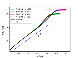
Figure 5: The scaled power spectrum of instantaneous currents, $L\tilde{S}_{\mathcal{J}}(f)/(2\chi)$, is plotted as a function of scaled frequency $L^{2}f/D$ for various chipping parameters and system sizes. The cyan solid line corresponds to $\lambda=0.25$ and $L=1000$, the magenta solid line corresponds to $\lambda=0.90$ and $L=1000$, the red solid line corresponds to $\lambda=0.25$ and $L=500$, and the green solid line corresponds to $\lambda=0.90$ and $L=500$, all at a global density of $\rho=1$. The blue dashed line shows $\tilde{y}^{1/2}$ scaling behavior in the low-frequency regime as in Eq.(99) and red dashed lines represent $L\tilde{S}_{\mathcal{J}}(f)/(2\chi)$ diverges as system size $2L-1$ at the high-frequency limit. The solid color lines represent the simulation results, while the black solid line represents the theoretical predictions of Eq.(97), which perfectly matches the simulation data.

According to Eq.(99), the power spectrum of the instantaneous currents displays a power-law behavior of $f^{\psi_{\mathcal{J}}}$ with an exponent of $\psi_{\mathcal{J}}=1/2$ in the low-frequency regime. Additionally, it can be inferred that in the temporal domain, the correlation of instantaneous current has a scaling behavior of $\langle\mathcal{J}_{0}(t)\mathcal{J}_{0}(0)\rangle\sim t^{-\psi_{\mathcal{J}}-1}$, which is qualitatively described by a $t^{-3/2}$ behavior.

III.5 Subsystem mass fluctuations

In previous sections, we have a detailed study on current-current dynamical correlation and its associated power spectrum of instantaneous current. In this section, we study the power spectrum of subsystem mass fluctuation. For that, we derive a two-point dynamic correlation of mass $C_{r}^{mm}(t,0)=\left\langle m_{i}(t)m_{i+r}(0)\right\rangle-\left\langle m_{i}(t)\right\rangle\left\langle m_{i+r}(0)\right\rangle$. By employing the microscopic update rule, we can derive the time evolution of $C_{r}^{mm}(t,0)\equiv C_{r}^{mm}(t)$ as follows:

$$\begin{aligned} \frac{d}{dt}C_{r}^{mm}(t)&=D\sum\limits_{k}\Delta_{0,k}\left\langle m_{k}(t)m_{r}(0)\right\rangle_{c}\\ &=D\sum\limits_{k}\Delta_{0,k}C_{k}^{mm}(t).\end{aligned}$$ (100)

The solution of above Eq.(100) can be written as Fourier representation as

$$\tilde{C}_{q}^{mm}(t)=e^{-D\omega_{q}t}\tilde{C}_{q}^{mm}(0),$$ (101)

where $\tilde{C}_{q}^{mm}$ is the Fourier transform of $C_{r}^{mm}$. The equal-time mass correlation $C_{r}^{mm}(0)$ corresponds to the steady-state mass-mass correlation $C_{r}^{mm}$ mentioned in Eq.(50). Notably, this correlation $C_{r}^{mm}$ has a direct connection with scaled subsystem-mass fluctuation,

$$\sigma_{M}^{2}\equiv\lim\limits_{l\to\infty}\frac{\left\langle M_{l}^{2}\right\rangle-\left\langle M_{l}\right\rangle^{2}}{l}=\sum\limits_{r=-\infty}^{r=\infty}C_{r}^{mm}=\frac{\chi}{D},$$ (102)

where boundary contribution of $C_{r}^{mm}$ has been neglected.

Note that, in the above equation, the mobility $\chi$ is defined purely from current fluctuations in the systems, when the particle hopping rates are strictly symmetric in either directions. Indeed, the essence of the MFT is that, for “gradient-type models”, the current fluctuations can be alternatively calculated using a slightly different approach where the hopping rates are biased in a certain direction; this amounts to applying a small biasing force in that direction so that the hopping rates become slightly asymmetric and a small current is generated in the system. Interestingly, this particular scheme leads to definition of another transport coefficient in the system, we call it an “operational” mobility, which characterizes the response of the systems (i.e., the small current generated) to a small force field $F$, which, for simplicity, assumed to be constant. Indeed, in Ref. [39], one of us previously introduced such a biasing force which modifies the original unbiased (symmetric) hopping rates of MCMs; of course, in the absence of the force $F$, we recover the original time-evolution equation of Eq.(6)). In that case, a time-evolution equation of local density, as opposed to the unbiased scenario as in Eq.(6)), is given by

$$\frac{d\rho_{i}}{dt}=\frac{\tilde{\lambda}}{2}(\rho_{i+1}-2\rho_{i}+\rho_{i-1})+\frac{\tilde{\lambda}^{2}}{12}F\left(\left\langle m_{i-1}^{2}\right\rangle-\left\langle m_{i+1}^{2}\right\rangle\right),$$ (103)

where $\rho_{i}=\left\langle m_{i}\right\rangle$. By scaling space and time as $x=i/L$ and $\tau=t/L^{2}$ and the (vanishingly) small biasing force as $F=\tilde{F}/L$, the time evolution equation for density field $\rho(x,\tau)$ as a function of the rescaled space and time variables can be expressed in terms of a continuity equation,

$$\begin{aligned} \partial_{\tau}\rho(x,\tau)&=-\partial_{x}\left[-D\partial_{x}\rho(x,\tau)+\chi_{op}\tilde{F}\rho(x,\tau)\right]\\ &=-\partial_{x}J(x,\tau),\end{aligned}$$ (104)

where the total local current $J=J_{diff}+J_{drift}$ is written as the sum of the diffusive current $J_{diff}=-D\partial_{x}\rho(x,\tau)$ and drift current $J_{drift}=\chi_{op}\tilde{F}$; here the two transport coefficients - the bulk-diffusion coefficient and the “operational” mobility are given by $D=\tilde{\lambda}/2$ and $\chi_{op}=\left\langle m_{i}^{2}\right\rangle/6$, respectively. The latter identity immediately implies, directly through Eq.(31), a simple fluctuation-response relation

$$\chi_{op}(\rho)\equiv\left[\frac{\partial J_{drift}}{\partial\tilde{F}}\right]_{\tilde{F}=0}=\sigma_{Q}^{2}\equiv\chi(\rho).$$ (105)

In other words, we have derived here a nonequilibrium version of the celebrated Green-Kubo relation for (near) equilibrium systems. We can immediately derive a version of another celebrated relation in equilibrium, called the Einstein relation, which connects the scaled mass fluctuation, the bulk-diffusion coefficient and the “operational” mobility, i.e.,

$$\chi_{op}\equiv\left[\frac{\partial J_{drift}}{\partial\tilde{F}}\right]_{\tilde{F}=0}=D\sigma^{2}_{M},$$ (106)

where we have used the already derived fluctuation relation [47] as given in Eq.(102); notably, the above equation is exact for MCMs and the above analysis constitutes a microscopic derivation of the relation. Furthermore, by using Eq.(85) and Eq. (102), we can immediately derive another nonequilibrium fluctuation relation, between fluctuation of mass and that of current, as expressed in the following equation,

$$\sigma^{2}_{M}=\frac{\sigma^{2}_{\mathcal{Q}}}{2D}.$$ (107)

It is not difficult to see that the above relation is nothing but a slightly modified version of the equilibrium-like Einstein relation as given in Eq. (106). While the above set of fluctuation relations is well established in the context of equilibrium systems, their existence in systems having a nonequilibrium steady state is not well understood. Indeed, a general theoretical understanding has emerged for nonequilibrium diffusive systems, which MCMs belong to, and it is desirable to prove such relations using exact microscopic calculations, which are still a formidable task even for the simplest class of models, i.e., the many-particle diffusive systems.

In order to solve Eq.(101), we must determine the value of the steady-state mass-mass correlation in Fourier mode, denoted as $C_{q}^{mm}$, which is given by:

$$C_{q}^{mm}=\frac{\chi}{D}\left(1+\frac{\omega_{q}}{2}\right).$$ (108)

Now, we substitute the above equation into Eq.(101) to obtain the solution of Eq.(101) as follows:

$$\tilde{C}_{q}^{mm}(t)=\frac{\chi}{D}e^{-D\omega_{q}t}\left(1+\frac{\omega_{q}}{2}\right).$$ (109)

Finally, using inverse Fourier transformation, we get

$$C_{r}^{mm}(t)=\frac{\chi}{D}\frac{1}{L}\sum\limits_{q}e^{-iqr}e^{-D\omega_{q}t}\left(1+\frac{\omega_{q}}{2}\right).$$ (110)

To calculate the asymptotic behavior at the single site level, we express the above expression by setting $r=0$ and write it in integral form as follows:

$$C_{0}^{mm}(t)\simeq\frac{\chi}{\pi D}\int\limits_{0}^{\pi}dqe^{-D\omega(q)t}\left[1+\frac{\omega(q)}{2}\right].$$ (111)

Now, we approximate $\omega(q)\approx q^{2}$ and perform a variable transformation $z=Dtq^{2}$ to simplify the above equation as follows:

$$C_{0}^{mm}(t)\simeq\frac{\chi}{\pi D\sqrt{4Dt}}\int\limits_{0}^{\pi}z^{-\frac{1}{2}}e^{-z}dz,$$ (112)

where subleading term $O(t^{-3/2})$ is neglected. After putting the value of the integral $\int_{0}^{\infty}z^{-\frac{1}{2}}e^{-z}dz=\sqrt{\pi}$ in the above equation, we obtain the asymptotic expression of dynamic correlation of mass at a single site as

$$C_{0}^{mm}(t)\simeq\frac{\chi}{D\sqrt{4\pi D}}t^{-\frac{1}{2}}.$$ (113)

We now consider a subsystem of size $l<L$ with a total mass $M_{l}(t)=\sum_{i=0}^{l-1}m_{i}(t)$ and calculate the unequal-time correlation of mass $C^{M_{l}M_{l}}(t,0)\equiv C^{M_{l}M_{l}}(t)$ as follows:

$$C^{M_{l}M_{l}}(t)=\left\langle\sum\limits_{i=0}^{l-1}m_{i}(t)\sum\limits_{j=0}^{l-1}m_{j}(0)\right\rangle_{c}.$$ (114)

Upon simplification of the above equation, we obtain,

$$C^{M_{l}M_{l}}(t)=lC_{0}^{mm}(t)+\sum\limits_{r=1}^{l-1}(l-r)\left[C_{r}^{mm}(t)+C_{-r}^{mm}(t)\right].$$ (115)

After substituting Eq.(110) into the previous equation and performing algebraic operations, we arrive at the subsequent expression,

$$C^{M_{l}M_{l}}(t)=\frac{\chi}{D}\frac{1}{L}\sum\limits_{q}e^{-D\omega_{q}t}\left(1+\frac{\omega_{q}}{2}\right)\frac{\omega_{lq}}{\omega_{q}}.$$ (116)

Now, we derive the temporal asymptotic behavior of the dynamic correlation of the subsystem mass $C^{M_{l}M_{l}}(t)$ as appeared in Eq.(116). At time $t=0$, it takes a maximum value and after that, it decays as a function of time $t$. To extract the time dependency, we isolate $C^{M_{l}M_{l}}(t)$ after its subtracted from its maximum value and then express the equation in an approximate integral form as mentioned below:

$$\begin{aligned} &C^{M_{l}M_{l}}(0)-C^{M_{l}M_{l}}(t)\\ &\simeq\frac{2\chi}{\pi D}\int\limits_{0}^{\pi}dq\left[1-e^{-D\omega(q)t}\right]\left[1+\frac{\omega(q)}{2}\right]\frac{1}{\omega(q)}.\end{aligned}$$ (117)

Again, we approximate $\omega(q)\approx q^{2}$ and perform a variable transformation $z=Dtq^{2}$ to simplify the above equation in the leading order as follows:

$$C^{M_{l}M_{l}}(0)-C^{M_{l}M_{l}}(t)\simeq\frac{\chi\sqrt{t}}{\pi\sqrt{D}}\int\limits_{0}^{\infty}z^{-\frac{3}{2}}(1-e^{-z})dz.$$ (118)

After putting the value of the integral $\int_{0}^{\infty}z^{-3/2}(1-e^{-z})dz=2\sqrt{\pi}$ in the above equation, we obtain the asymptotic expression of dynamic correlation of the subsystem mass as

$$C^{M_{l}M_{l}}(t)-C^{M_{l}M_{l}}(0)\simeq-\frac{2\chi}{\sqrt{\pi D}}t^{\frac{1}{2}}.$$ (119)

Now, after taking the Fourier transform of the Eq.(116), we can express the power spectrum of the subsystem mass fluctuation $S_{M_{l}}(f)$ as follows:

$$S_{M_{l}}(f) =\lim\limits_{T\to\infty}\int\limits_{-T}^{T}dt~{}C^{M_{l}M_{l}}(t,0)e^{2\pi ift}.$$ (120)

Upon completing the aforementioned integration, we have derived the subsequent expression,

$$S_{M_{l}}(f)=\frac{2\chi}{L}\sum\limits_{q}\left(1+\frac{\omega_{q}}{2}\right)\frac{\omega_{lq}}{\omega_{q}^{2}D^{2}+4\pi^{2}f^{2}},$$ (121)

where $\omega_{q}=2(1-\cos q)$, with $q=2\pi n/L$ and $n=1,2,\cdots,L-1$. We would like to present an additional scaling function, denoted as $\mathcal{F}$, that links $S_{M_{l}}(f)$ in the following manner:

$$\mathcal{F}\left(\frac{L^{2}f}{D}\right) =\frac{D^{2}}{2\chi L^{3}}S_{M_{l}}(f)$$ (122)

$$=\lim_{L\to\infty}\sum\limits_{q}\left(1+\frac{\omega_{q}}{2}\right)\frac{\omega_{lq}}{L^{4}\omega_{q}^{2}+4\pi^{2}(L^{2}f/D)^{2}}.$$

Additionally, it is worth noting that the sub-system mass power spectrum $S_{M_{l}}(f)$ can be represented by an integral, as stated below,

$$\mathcal{F}(\tilde{y}) \simeq\lim\limits_{L\to\infty}\frac{L}{\pi}\int\limits_{2\pi/L}^{\pi}dq\left[1+\frac{\omega(q)}{2}\right]\frac{\omega(lq)}{4\pi^{2}\tilde{y}^{2}+L^{4}\omega(q)^{2}}.$$ (123)

For a large subsystem size $1\ll l<L$, the function $\omega(lq)$ exhibits high-frequency oscillations with values in the range of $[0,4]$, leading to an approximation of $\omega(lq)\approx 2$. Additionally, we can make use of the transformation $z=\omega(q)L^{2}$ and then taking $L\to\infty$, we obtain the following expression,

$$\mathcal{F}(\tilde{y})\simeq\frac{1}{4\pi^{3}\tilde{y}^{2}}\int\limits_{0}^{\infty}\frac{dz}{z^{1/2}\left(1+\frac{z^{2}}{4\pi^{2}\tilde{y}^{2}}\right)}.$$ (124)

After performing the above integral, we obtain the asymptotic expression of the scaled power spectrum of the subsystem mass fluctuation as follows:

$$\mathcal{F}(\tilde{y})\simeq\frac{(\tilde{y}\pi)^{-\frac{3}{2}}}{4}.$$ (125)

This implies that in the low-frequency regime, the power spectrum of the subsystem mass follows a power-law behavior $f^{-\psi_{M}}$ with an exponent of $\psi_{M}=3/2$. It is also evident that in the temporal domain, the correlation of the subsystem mass $\langle M_{l}(t)M_{l}(0)\rangle_{c}$ scales as $t^{\psi_{M}-1}$, which is qualitatively a $t^{1/2}$ behavior.

Fig. 6 displays the scaled sub-system mass power spectrum $D^{2}\tilde{S}_{M_{l}}(f)/(2\chi L^{3})$ as a function of the scaled frequency $L^{2}f/D$ for various chipping parameters and system sizes, along with theoretical predictions. The power spectrum exhibits notable scaling behaviors in the low-frequency range, with the red dashed line indicating a $\tilde{y}^{-3/2}$ scaling behavior. The simulation results (solid color lines) are in excellent agreement with the theoretical predictions (black solid line).

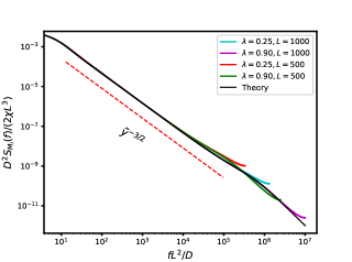
Figure 6: The scaled subsystem mass power spectrum, $D^{2}\tilde{S}_{M_{l}}(f)/(2\chi L^{3})$, is plotted as a function of the scaled frequency $L^{2}f/D$ for various chipping parametre and system sizes. The lines, colored cyan ($\lambda=0.25$, $L=1000$), magenta ($\lambda=0.90$, $L=1000$), red ($\lambda=0.25$, $L=500$), and green ($\lambda=0.90$, $L=500$), represent simulation data, all obtained at a global density of $\rho=1$. In the low-frequency range, the red dashed line demonstrates a scaling behavior of $\mathcal{F}(\tilde{y})$ as $\tilde{y}^{-3/2}$ [as in Eq.(125)]. The black solid line corresponds to theoretical predictions [as mentioned in Eq.(122)], providing an excellent match with the simulation data for that system size.

IV Model: MCM II

In this section, we apply a similar theoretical framework as developed in the previous section. In the case of MCM II, a site is selected randomly, and a portion of the chipped-off mass is transferred either to the right nearest neighbor or the left nearest neighbor, with the remaining chipped-off mass being deposited back onto the same site. This dynamic behavior results in the absence of nearest-neighbor correlations, simplifying the calculation of dynamic correlations. Since we have already provided an analytical theory for MCM I model, we now present the significant findings for MCM II model.

IV.1 Time-integrated current fluctuation

Importantly, for MCM II, the time-integrated bond-current fluctuation follows the functional form as mentioned in Eq.(126). In this case, the strength of the fluctuating current is characterized by $\Gamma_{r}=2\chi\delta_{0,r}$, where the bulk diffusion coefficient is given by $D=\frac{\tilde{\lambda}}{4}$, and the mobility $\chi$ remains identical to that of MCM I. Indeed, it’s worth highlighting that for this model, MCM II, both the steady-state density correlation $C_{r}^{mm}$ and the strength of the fluctuating current $\Gamma_{r}$ are short-ranged, indicating a lack of nearest-neighbor correlation (as indicated in Table I. Additionally, it’s noteworthy that $\Gamma_{r}$ and $C_{r}^{mm}$ are related by a scaling factor represented by the bulk diffusivity $D$, as demonstrated in Eq.(34), and this relationship holds true for this model as well.

For MCM II, we proceed to calculate the time-integrated bond-current fluctuation $C_{0}^{QQ}(t,t)$ for equal time $t^{\prime}=t=T$ and in the same space, i.e., $r=0$. The resulting expression is as follows:

$$\langle\mathcal{Q}^{2}(T)\rangle=\frac{2\chi T}{L}+\frac{2\chi}{L}\sum\limits_{n=1}^{L-1}\frac{(1-e^{-D\omega_{n}T})}{D\omega_{n}},$$ (126)

where $\omega_{n}=2(1-\cos(2\pi n/L))$, with $n=0,1,\cdots,L-1$. If we take the $T\to\infty$ limit first in the above equation, we get the following expression,

$$\langle\mathcal{Q}^{2}(T)\rangle\simeq\frac{2\chi T}{L}+\frac{\chi L}{6D}=\frac{2\chi T}{L}\left[1+{\cal O}\left(\frac{L^{2}}{DT}\right)\right].$$ (127)

It is worth noting that the term $\chi L/6D$ in the above equation can be safely neglected since the leading contribution will arise from the $2\chi T/L$ term as $T\gg L^{2}$. In the smaller time regime where $DT\ll 1$, Eq.(126) can be simplified as follows:

$$\langle\mathcal{Q}^{2}(T)\rangle=\Gamma_{0}T=2\chi T,$$ (128)

where the strength of the fluctuating current $\Gamma_{0}$ is equal to $2\chi$, which differs from the value found in the first model, MCM I (as demonstrated in Eq.(33)). Furthermore, it’s worth highlighting that in the scaling regime where $DT\gg 1$, we’ve observed that the scaling function $\mathcal{W}(y)$, with the scaling variable $y=DT/L^{2}$, maintains the same form as presented in Eq.(68), as observed in MCM I. In Figure 7, we present the time-integrated bond-current fluctuation, denoted as $\langle\mathcal{Q}_{i}^{2}(T)\rangle$, as a function of time $T$ in the top panel. We highlight the early-time behavior of $\langle\mathcal{Q}^{2}(T)\rangle$, which scales as $\Gamma_{0}T$ and is described in Eq.(128). Additionally, in the bottom panel of this figure, we showcase the scaled fluctuation of the time-integrated current, represented as $\langle\mathcal{Q}_{i}^{2}(T)\rangle D/(2\chi L)$, as a function of the scaled time $DT/L^{2}$. We include guiding lines that illustrate the asymptotic behavior of the scaling function $\mathcal{W}(y)$.

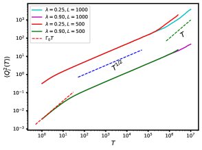
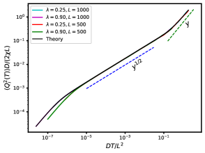
Figure 7: In top panel:We present the time-integrated bond-current fluctuation, denoted as $\langle\mathcal{Q}_{i}^{2}(T)\rangle$, plotted as a function of time $T$ for various chipping parameters and system sizes. For both this panel, the cyan ($\lambda=0.25$, $L=1000$), magenta ($\lambda=0.90$, $L=1000$), red ($\lambda=0.25$, $L=500$), and green ($\lambda=0.90$, $L=500$) lines represent simulation data at a global density of $\rho=1$. The red dashed line corresponds to the behavior $\Gamma_{0}T$ for $\lambda=0.90$ (refer to Eq.(128)), while the blue and green dashed lines represent sub-diffusive growth, approximately scaling as $\sim T^{1/2}$, and diffusive growth, approximately scaling as $\sim T$, respectively, as discussed in Eq.(129) In bottom panel: The plot displays the scaled time-integrated bond-current fluctuation, $\langle\mathcal{Q}_{i}^{2}(T)\rangle D/(2\chi L)$, as a function of scaled time $DT/L^{2}$ for various chipping parameter and system sizes. The two dashed lines serve as guides, indicating that $\mathcal{W}(y)$ exhibits sub-diffusive behavior as $\sim y^{1/2}$ (in blue) at early times, followed by diffusive growth as $\sim y$ (in green) at later times [as in Eq.(70)]. The solid color lines illustrate the simulation results, while the black solid line represents the theoretical results obtained from Eq.(126) upon suitable scaling, and this theoretical curve perfectly matches the simulation data.

The overall growth of the time-integrated bond-current fluctuation exhibits three distinct asymptotic regimes, as described below:

$$\langle\mathcal{Q}^{2}(T)\rangle=\begin{cases}2\chi T&\text{for}~{}DT\ll 1\\ \frac{2\chi}{\sqrt{D\pi}}T^{\frac{1}{2}}&\text{for}~{}1\ll DT\ll L^{2}\\ \frac{2\chi T}{L}&\text{for}~{}DT\gg L^{2}\end{cases}$$ (129)

IV.2 Instantaneous bond-current fluctuations

Using the theory presented in Section III, we have computed the power spectrum of the instantaneous bond current $\mathcal{J}_{i}(t)$ in MCM II. The expression for the power spectrum is provided below:

$$\tilde{S}_{\mathcal{J}}(f)=\frac{2\chi(\rho)}{L}\sum\limits_{q}\frac{4\pi^{2}f^{2}}{D^{2}\omega_{q}^{2}+4\pi^{2}f^{2}},$$ (130)

where, $\omega_{q}=2(1-\cos q)$, with $q=2\pi n/L$ and $n=1,2,\cdots,L-1$. The above expression exhibits an asymptotic behavior $\mathcal{H}(\tilde{y})\sim\tilde{y}^{1/2}$ in the lower frequency regime, similar to MCM I as mentioned in Eq.(99). Furthermore, $\mathcal{H}(\tilde{y})$ diverges as $L-1$ in the limit $\tilde{y}\to\infty$ (much larger than $L^{2}$).

In Figure 8, the scaled power spectrum of the instantaneous bond current, represented as $L\tilde{S}_{\mathcal{J}}(f)/(2\chi)$, plotted against the scaled frequency $L^{2}f/D$. Both simulation and theoretical results are shown, and they exhibit a perfect match. Additionally, in the lower frequency range, we have included a guiding line $\sim\tilde{y}^{1/2}$, which is obtained from the integral representation of Eq.(130). This behavior is consistent with what was mentioned earlier in the context of MCM I.

Figure 8: The scaled power spectrum of instantaneous currents, $L\tilde{S}_{\mathcal{J}}(f)/(2\chi)$, is plotted as a function of scaled frequency $L^{2}f/D$ for various chipping parameters and system sizes. The cyan solid line corresponds to $\lambda=0.25$ and $L=1000$, the magenta solid line corresponds to $\lambda=0.90$ and $L=1000$, the red solid line corresponds to $\lambda=0.25$ and $L=500$, and the green solid line corresponds to $\lambda=0.90$ and $L=500$, all at a global density of $\rho=1$. The blue dashed line shows $\tilde{y}^{1/2}$ scaling behavior in the low-frequency regime as in Eq.(99) and red dashed lines represent $L\tilde{S}_{\mathcal{J}}(f)/(2\chi)$ diverges as system size $L-1$ at the high-frequency limit. The solid color lines represent the simulation results, while the black solid line represents the theoretical predictions of Eq.(130) upon suitable scaling, which fully matches the simulation data.

IV.3 Subsystem mass fluctuations

For MCM II, we have also computed another temporal quantity known as the sub-system mass power spectrum $S_{M_{l}}(f)$. This quantity is expressed as a summation as below:

$$S_{M_{l}}(f)=\frac{2\chi}{L}\sum\limits_{q}\frac{\omega_{vq}}{\omega_{q}^{2}D^{2}+4\pi^{2}f^{2}}.$$ (131)

Additionally, we have calculated the scaling function $\mathcal{F}(\tilde{y})$ associated with the power spectrum of the subsystem mass. Notably, it exhibits a $\tilde{y}^{-3/2}$ behavior in the low-frequency limit, mirroring the behavior observed in model MCM I as previously mentioned in Eq.(125). In Figure 9, the scaled subsystem mass power spectrum, denoted as $D^{2}\tilde{S}_{M_{l}}(f)/(2\chi L^{3})$, plotted against the scaled frequency $L^{2}f/D$ for various chipping parameters and system sizes. The red dashed line exhibits a $\tilde{y}^{-3/2}$ scaling behavior in the low-frequency regime. The solid color lines represent the simulation results, and the black solid line corresponds to the theoretical predictions from Eq.(131), which matches the simulation data when suitably scaled.

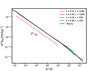
Figure 9: The scaled subsystem mass power spectrum, $D^{2}\tilde{S}_{M_{l}}(f)/(2\chi L^{3})$, is plotted as a function of scaled frequency $L^{2}f/D$ for various chipping parametre and system sizes. The cyan solid line corresponds to $\lambda=0.25$ and $L=1000$, the magenta solid line corresponds to $\lambda=0.90$ and $L=1000$, the red solid line corresponds to $\lambda=0.25$ and $L=500$, and the green solid line corresponds to $\lambda=0.90$ and $L=500$, all at a global density of $\rho=1$. The red dashed line shows a $\tilde{y}^{-3/2}$ scaling behavior in the low-frequency regime. The solid color lines represent the simulation results, while the black solid line represents the theoretical predictions of Eq.(131) upon suitable scaling, which matches the simulation data.

V MCM III

In this section, we have computed the dynamic correlation for MCM III, which has been previously investigated to comprehend the distribution of wealth in a population[48, 49]. In this model, each site retains a fraction of its own mass, and the remaining mass is distributed among its nearest neighbor sites. The distribution of the mixed masses among these sites is randomized. It is important to note that the dynamic correlations for this model, MCM II, turn out to be similar to those of model MCM II upon appropriate scaling. This similarity arises from the fact that both of these models exhibit similar density correlation behaviors due to their respective microscopic dynamics.

V.1 Time-integrated current fluctuation

The time-integrated bond current fluctuation in MCM III takes on an identical form to that of MCM II, as shown in Eq.(126). What stands out is that the strength of the fluctuating current $\Gamma_{0}$ and the conductivity $\chi$ are the same as in MCM II. The key distinction lies in the bulk diffusivity, which is given by $D=\frac{\tilde{\lambda}}{2}$ for MCM III.

In Figure 10, we present the time-integrated bond-current fluctuation, denoted as $\langle\mathcal{Q}_{i}^{2}(T)\rangle$, as a function of time $T$ in the top panel. The early-time behavior of $\langle\mathcal{Q}^{2}(T)\rangle$, which scales as $\Gamma_{0}T$ according to Eq.(128), is highlighted. In the bottom panel, we display the scaled fluctuation of the time-integrated current, $\langle\mathcal{Q}_{i}^{2}(T)\rangle D/(2\chi L)$, as a function of scaled time $DT/L^{2}$. Solid color lines represent simulation results, while the black solid line represents the theoretical prediction obtained from Eq.(126), which closely matches the simulation data when appropriately scaled. Guiding lines illustrate the asymptotic behavior of the scaling function $\mathcal{W}(y)$.

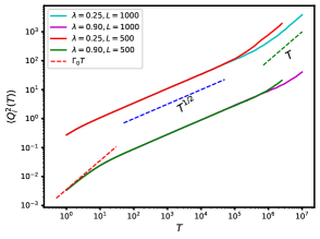
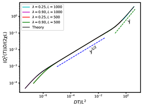
Figure 10: In top panel: The time-integrated bond-current fluctuation, $\langle\mathcal{Q}_{i}^{2}(T)\rangle$, plotted as a function of time $T$ for various chipping parameter and system sizes. For both this panel, the cyan ($\lambda=0.25$, $L=1000$), magenta ($\lambda=0.90$, $L=1000$), red ($\lambda=0.25$, $L=500$), and green ($\lambda=0.90$, $L=500$) lines lines represent simulation data for global density $\rho=1$. The red dashed line represents the behavior $\Gamma_{0}T$ for $\lambda=0.90$ [see Eq(128)], while the blue and green dashed lines represent sub-diffusive $\sim T^{1/2}$ and diffusive $\sim T$ growth, respectively, as mentioned in Eq.(129). In bottom panel: The plot shows the scaled time-integrated bond-current fluctuation, $\langle\mathcal{Q}_{i}^{2}(T)\rangle D/(2\chi L)$, as a function of scaled time $DT/L^{2}$ for different chipping parameter and system sizes. The two dashed lines serve as guides, indicating that $\mathcal{W}(y)$ exhibits sub-diffusive behavior as $\sim y^{1/2}$ (in blue) at early times, followed by diffusive growth as $\sim y$ (in green) at later times [as in Eq.(70)]. Solid color lines represent simulation results, while the black solid line represents the theoretical prediction obtained from Eq.(126), which perfectly matches the simulation data when suitably scaled.

V.2 Instantaneous bond-current fluctuations

For MCM III, we have calculated the power spectrum of the instantaneous current, and interestingly, it exhibits the same form as mentioned in Eq.(130), with $D=\lambda/2$ and the conductivity being the same as above mentioned MCMs (MCM I and MCM II).

In Fig. 11, the scaled power spectrum of the instantaneous bond current, represented as $L\tilde{S}_{\mathcal{J}}(f)/(2\chi)$, plotted against the scaled frequency $L^{2}f/D$. Both simulation and theoretical results are shown, and they exhibit a perfect match. Additionally, in the lower frequency range, we have included a guiding line $\sim\tilde{y}^{1/2}$. This behavior is consistent with what was mentioned earlier in the context of MCM I [see Eq.(99)]. Notably, both models MCM II and MCM III show identical behavior in the scaled plot, both from simulation and theory, indicating a strong agreement between the two.

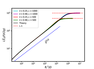
Figure 11: The scaled power spectrum of instantaneous currents, $L\tilde{S}_{\mathcal{J}}(f)/(2\chi)$, is plotted as a function of scaled frequency $L^{2}f/D$ for various chipping parameters and system sizes. The cyan solid line corresponds to $\lambda=0.25$ and $L=1000$, the magenta solid line corresponds to $\lambda=0.90$ and $L=1000$, the red solid line corresponds to $\lambda=0.25$ and $L=500$, and the green solid line corresponds to $\lambda=0.90$ and $L=500$, all at a global density of $\rho=1$. The blue dashed line shows $\tilde{y}^{1/2}$ scaling behavior in the low-frequency regime and the red dashed lines represent the power spectrum diverges as $L-1$ at the high-frequency limit. The solid color lines represent the simulation results, while the black solid line represents the theoretical predictions of Eq.(130) upon suitable scaling, which fully matches the simulation data.

V.3 Subsystem Mass fluctuations

Additionally, we have calculated the power spectrum of the subsystem mass, and remarkably, it follows the same form as mentioned in Eq.(131). In Figure 12, we plot the scaled subsystem mass power spectrum, denoted as $D^{2}\tilde{S}_{M_{l}}(f)/(2\chi L^{3})$, against the scaled frequency $L^{2}f/D$ for various chipping parameters and system sizes. Solid color lines represent simulation results, and the black solid line corresponds to theoretical predictions from Eq.(131), matching the simulation data when suitably scaled. The red dashed line shows a $\tilde{y}^{-3/2}$ scaling behavior at low frequencies, agreeing with MCM I [Eq.(125)].

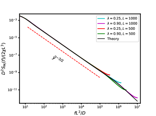
Figure 12: The scaled subsystem mass power spectrum, $D^{2}\tilde{S}_{M_{l}}(f)/(2\chi L^{3})$, is plotted as a function of scaled frequency $L^{2}f/D$ for various chipping parameter and system sizes. The cyan solid line corresponds to $\lambda=0.25$ and $L=1000$, the magenta solid line corresponds to $\lambda=0.90$ and $L=1000$, the red solid line corresponds to $\lambda=0.25$ and $L=500$, and the green solid line corresponds to $\lambda=0.90$ and $L=500$, all at a global density of $\rho=1$. The red dashed line shows a $\tilde{y}^{-3/2}$ scaling behavior in the low-frequency regime. The solid color lines represent the simulation results, while the black solid line represents the theoretical predictions of Eq.(131) upon suitable scaling, which matches the simulation data.

VI Comparison of models

In this section, we present a comprehensive comparative study of various dynamical quantities for the three models: MCM I, MCM II, and MCM III. Specifically, we investigate the scaled time-integrated bond-current fluctuation $\mathcal{W}(y)$ as a function of scaled time $y=DT/L^{2}$, the scaled power spectrum of instantaneous currents $\mathcal{H}(\tilde{y})$, and the scaled subsystem mass power spectrum $\mathcal{F}(\tilde{y})$ as a function of scaled frequency $\tilde{y}=fL^{2}/D$ for these three models. In Fig.(13), we present comparative plots of these dynamical quantities for the three models. Remarkably, despite the different microscopic dynamics of the models, we find that there exists an appropriate scaling regime, where all three models in fact exhibit qualitatively quite similar behavior. This observation suggests that certain universal features are shared among these models, and presumably diffusive systems in general, even when the underlying dynamical mechanisms are completely different.

Furthermore, we note that outside the scaling regime, deviations are observed between the model with nearest neighbor correlation (MCM I) and the models without nearest neighbor correlation (MCM II and MCM III). These deviations are accurately captured in both the simulation data and theoretical predictions, providing insights into the distinct dynamical properties of each model.

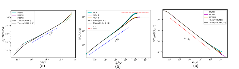
Figure 13: (a) Scaled time-integrated bond-current fluctuation, $\langle\mathcal{Q}_{i}^{2}(T)\rangle D/(2\chi L)$, as a function of scaled time $DT/L^{2}$ for three models: MCM I (blue solid line), MCM II (magenta solid line), and MCM III (orange solid line). The two dashed lines serve as guides, indicating that $\mathcal{W}(y)$ exhibits sub-diffusive behavior as $\sim y^{1/2}$ (in blue) at early times, followed by diffusive growth as $\sim y$ (in green) at later times. (b) Scaled power spectrum of instantaneous currents, $L\tilde{S}_{\mathcal{J}}(f)/(2\chi)$, plotted as a function of scaled frequency $L^{2}f/D$ for various chipping parameter and system sizes. The blue dashed line represents the $\tilde{y}^{1/2}$ scaling behavior of $\mathcal{H}(\tilde{y})$ in the low-frequency regime. In contrast, the power spectrum exhibits divergence, reaching $2L-1$ (red dashed line) for MCM I and $L-1$ (lime dashed line) for MCM II and MCM III in the high-frequency limit. (c) Scaled subsystem mass power spectrum, $D^{2}\tilde{S}_{M_{l}}(f)/(2\chi L^{3})$, plotted as a function of scaled frequency $L^{2}f/D$ for various chipping parameters and system sizes. The red dashed line shows a $\tilde{y}^{-3/2}$ scaling behavior of $\mathcal{F}(\tilde{y})$ in the low-frequency regime. In all of these panels, we have used a fixed chipping parameter $\lambda=0.5$, global density $\rho=1.0$, and a system size of $L=1000$. Simulation data for MCM I, MCM II, and MCM III are represented by blue, magenta, and orange solid lines, respectively. Black dashed lines correspond to MCM I theory, while black solid lines represent MCM II and MCM III theory, which are identical.

Quantity	MCM I	MCM II	MCM III
Bulk-diffusivity: D	$\frac{\tilde{\lambda}}{2}$	$\frac{\tilde{\lambda}}{4}$	$\frac{\tilde{\lambda}}{2}$
Mobility: $\mathbf{\chi}$	$\frac{\tilde{\lambda}^{2}\rho^{2}}{2(3-2\tilde{\lambda})}$	$\frac{\tilde{\lambda}^{2}\rho^{2}}{2(3-2\tilde{\lambda})}$	$\frac{\tilde{\lambda}^{2}\rho^{2}}{2(3-2\tilde{\lambda})}$
Density correlation: $\mathbf{C_{r}^{mm}}$	$\frac{\tilde{\lambda}\rho^{2}}{2(3-2\tilde{\lambda})}[4\delta_{0,r}-\delta_{r,1}-\delta_{r,-1}]$	$\frac{2\tilde{\lambda}}{(3-2\tilde{\lambda})}\rho^{2}\delta_{0,r}$	$\frac{\tilde{\lambda}}{(3-2\tilde{\lambda})}\rho^{2}\delta_{0,r}$
$\mathbf{\Gamma_{r}}$	$\frac{\tilde{\lambda}^{2}\rho^{2}}{2(3-2\tilde{\lambda})}[4\delta_{0,r}-\delta_{r,1}-\delta_{r,-1}]$	$\frac{\tilde{\lambda}^{2}\rho^{2}}{(3-2\tilde{\lambda})}\delta_{r,0}$	$\frac{\tilde{\lambda}^{2}\rho^{2}}{(3-2\tilde{\lambda})}\delta_{r,0}$
$\mathbf{A_{r}}$	$\frac{\tilde{\lambda}^{2}\rho^{2}}{4(3-2\tilde{\lambda})}[-5(\delta_{r,0}-\delta_{r,-1})+(\delta_{r,1}-\delta_{r,-2})]$	$-\frac{1}{2}\frac{\tilde{\lambda}^{2}\rho^{2}}{(3-2\tilde{\lambda})}(\delta_{r,0}-\delta_{r,-1})$	$-\frac{1}{2}\frac{\tilde{\lambda}^{2}\rho^{2}}{(3-2\tilde{\lambda})}(\delta_{r,r}-\delta_{r,-1})$
$\mathbf{\tilde{f}_{q}}$	$-\frac{\tilde{\lambda}^{2}\rho^{2}}{2(3-2\tilde{\lambda})}(1-e^{-iq})\Big{(}1+\frac{w_{q}}{2}\Big{)}$	$-\frac{\tilde{\lambda}^{2}\rho^{2}}{2(3-2\tilde{\lambda})}(1-e^{-iq})$	$-\frac{\tilde{\lambda}^{2}\rho^{2}}{2(3-2\tilde{\lambda})}(1-e^{-iq})$

Table 1: We have highlighted key quantities related to dynamical correlations in these three models: MCM I, MCM II, and MCM III. These quantities include transport coefficients such as bulk diffusivity $D$ and mobility $\chi$. Additionally, we have mentioned steady-state density correlation $C_{r}^{mm}$, the strength of fluctuating current $\Gamma_{r}$, the source term in the time evolution equation of mass-current correlation at equal times $A_{r}$, and its Fourier mode $\tilde{f}_{q}$. These quantities are essential for deriving dynamical correlations in these models.

Table I provides a concise overview of the similarities and differences among these three models in terms of their key parameters and quantities related to dynamical correlations. To begin with, it highlights the transport coefficients, bulk diffusion coefficient $D$, and mobility $\chi$ for each model. Notably, $D$ is constant (indepndent of density) for all three models; however, the mobility $\chi$ is density dependent (proportional to density square). The table displays the density correlation function $C_{r}^{mm}$ for these models. MCM I possess nearest-neighbor correlations, whereas MCM II and MCM III lack such correlations. The table also presents the strength $\Gamma_{r}$ of fluctuating (“noise”) current for the models, with each model of the models having a distinct value. However, it is important to note that the relationship $\Gamma_{r}=C_{r}^{mm}/2D$ holds true for all models; presumably this relation is valid for diffusive systems in general. Lastly, the table compares the source term $A_{r}$ in the time evolution equation of mass-current correlation. For completeness, we also provide the Fourier modes of this source term, denoted as $\tilde{f}_{q}$, which proves to be useful in the explicit calculations of various dynamic quantities.

VII summary and Conclusion

In this paper, we exactly calculate dynamic correlation functions for mass and current in a broad class of one dimensional conserved-mass transport processes, called mass chipping models (MCMs). These systems violate detailed balance and have nontrivial spatial structures; indeed, their steady state measures are not described by the Boltzmann-Gibbs distribution, and a priori not known. Overall we find three temporal growth regimes for the fluctuation of the time-integrated bond current. Initially, for all three models, the time-integrated current fluctuation grows linearly with time $T$, with a proportionality factor of $\Gamma_{0}$, which, however, is a model-dependent quantity. In the intermediate, but large, time regime $1/D\ll T\ll L^{2}/D$, with $D$ being the bulk diffusion coefficient, we found subdiffusive - $T^{1/2}$ - growth of the current fluctuation where the density-dependent prefactor of $T^{1/2}$ is exactly determined. This was again followed by a linear or diffusive growth of current fluctuation in the large diffusive time region, $T\gg L^{2}$. Furthermore, we exactly calculate a model independent scaling function $\mathcal{W}(y)\equiv D\langle\mathcal{Q}_{i}^{2}(T)\rangle/2\chi L$ as a function of a scaling variable $y=DT/L^{2}$, where $D$, $\chi$ and $L$ are the bulk-diffusion coefficient, mobility, and system size $L$, respectively.

We calculate the dynamic correlation function for the instantaneous current and show that the correlation function decays as $t^{-3/2}$; notably, the correlation function has a delta-correlated part at $t=0$ and its magnitude for $t>0$ is negative. Indeed the negative part of the current correlation function is directly responsible for the subdiffusive growth of the bond current fluctuation in the thermodynamic limit. The power-law behavior of dynamic current correlations is consistent with the exact calculation of the current power spectrum, $\tilde{S}_{\mathcal{J}}(f)$, which has a low-frequency asymptotic behavior $\tilde{S}_{\mathcal{J}}(f)\sim f^{\psi_{\mathcal{J}}}$ with $\psi_{\mathcal{J}}=1/2$. Furthermore, we exactly obtain the scaling function which $\mathcal{H}(\tilde{y})$, which represents the rescaled power spectrum of the current $L\tilde{S}_{\mathcal{J}}(f)/2\chi$ as a function of the scaled variable $\tilde{y}=fL^{2}/D$.

We also calculate the scaled subsystem mass fluctuation, which is shown to be identically equal to the suitably scaled dynamic fluctuation of the space-time integrated current $\mathcal{Q}_{sub}(l,T)$, divided by factor of $2D$ - $D$ being the bulk-diffusion coefficient [see Eq.(107)]. This particular fluctuation relation in the context of MCMs is nothing but a slightly modified, nonequilibrium version of the celebrate equilibrium Einstein relation. It should be noted that the fluctuation relation requires the intensive fluctuation of space-time integrated current to be calculated in the thermodynamic limit, i.e., by first taking the limit of the infinite subsystem size limit $l\rightarrow\infty$, followed by the limit of infinite time $T\rightarrow\infty$. In this specific order of limits, we also show that $\lim_{l\rightarrow\infty}\lim_{T\rightarrow\infty}\langle\mathcal{Q}_{sub}^{2}(l,T)\rangle/lT$ is identically equal to the spatial sum of the strength $\Gamma_{r}$ of the fluctuating bond current. As a simple consequence of the Einstein relation, the correlation functions of mass and fluctuating current are related by $C_{r}^{mm}=\Gamma_{r}/2D$. We also calculate the unequal-time correlation function of the total mass of a subsystem and its power spectrum $S_{M_{l}}$, which decays as $S_{M_{l}}\sim f^{-\psi_{M}}$, with $\psi_{M}=3/2$, consistent with the scaling relation $\psi_{\mathcal{J}}=2-\psi_{M}$ [44]. The scaled power spectrum of subsystem mass, $D^{2}S_{M_{l}}(f)/2\chi L^{3}$, can also be expressed in terms of a scaling function $\mathcal{F}(\tilde{y})$ with scaling variable $\tilde{y}=fL^{2}/D$.

Notably, the qualitative behavior of time-integrated bond-current fluctuations for all three models are similar, though the prefactors of the temporal growth laws depend on the details of the dynamical rules. In the small-frequency (large-time) domain, the prefactors of the intermediate-time subdiffusive and long-time diffusive growth of the bond current fluctuations can be expressed in terms of the bulk-diffusion coefficient and the particle mobility. However, the large-frequency behavior is not universal in the sense that they depend on the local microscopic properties. More specifically, the different spatial structures of these models manifest in the small-time growth of the time-integrated bond-current fluctuation $\langle\mathcal{Q}^{2}_{i}(T)\rangle\simeq\Gamma_{0}T$, where $\Gamma_{0}$ is proportional to the single-site mass fluctuation $\langle m_{i}^{2}\rangle$, being considerably different in thse models.

A few remarks are in order. Characterizing the dynamic properties of interacting-particle systems through microscopic calculations is an important, though difficult, problem in statistical physics. The variants of mass chipping models discussed here have nontrivial steady states, that, unlike the SEP on a periodic domain, are not described by the Boltzmann-Gibbs distribution and, moreover, a-priori unknown. As mentioned above, depending on their dynamical rules, these models differ from each other in the details of their spatial structures. Model MCM I possesses nonzero spatial correlations, whereas MCM II and III have vanishing neighboring correlations. However all these models share one noteworthy aspect in common: The bulk-diffusion coefficient, like in the SEP [35], is independent of density. In fact, this is precisely why the hierarchy of current and mass correlations closes and thus the models are exactly solvable. Despite the fact that the mass chipping models have a nontrivial steady state, these models, due to their simple dynamical rules, do not exhibit a phase transition, or any singularities in the transport coefficients. However, through simple variations in the dynamical rules, it is possible to have nontrivial (singular) macroscopic behavior in some of the variants of these models. Indeed, it would be quite interesting to characterize the dynamic properties of current and mass through microscopic calculations in higher dimensions, for systems with more than one conserved density [34] and when the transport properties are singular or anomalous [44].

References

- Friedlander and Marlow [1977] S. K. Friedlander and W. H. Marlow, Smoke, Dust and Haze: Fundamentals of Aerosol Behavior, Physics Today 30, 58 (1977).
- Kipnis et al. [1982] C. Kipnis, C. Marchioro, and E. Presutti, Heat flow in an exactly solvable model, J. Stat. Phys. 27, 65 (1982).
- Liu et al. [1995] C.-H. Liu, S. R. Nagel, D. A. Schecter, S. N. Coppersmith, S. Majumdar, O. Narayan, and T. A. Witten, Force fluctuations in bead packs, Science 269, 513 (1995).
- Coppersmith et al. [1996] S. N. Coppersmith, C. h. Liu, S. Majumdar, O. Narayan, and T. A. Witten, Model for force fluctuations in bead packs, Phys. Rev. E 53, 4673 (1996).
- Scheidegger [1967] A. E. Scheidegger, A stochastic model for drainage patterns into an intramontane treinch, International Association of Scientific Hydrology. Bulletin 12, 15 (1967).
- Dutta and Kumar Sinha [2015] A. Dutta and D. Kumar Sinha, Turnover of the actomyosin complex in zebrafish embryos directs geometric remodelling and the recruitment of lipid droplets, Sci. Rep. 5, 1 (2015).
- Chowdhury et al. [2000] D. Chowdhury, L. Santen, and A. Schadschneider, Statistical physics of vehicular traffic and some related systems, Physics Reports 329, 199 (2000).
- Yakovenko and Rosser [2009] V. M. Yakovenko and J. B. Rosser, Colloquium: Statistical mechanics of money, wealth, and income, Rev. Mod. Phys. 81, 1703 (2009).
- Rajesh R. [2000] M. S. Rajesh R., Conserved mass models and particle systems in one dimension, Journal of Statistical Physics 99, 943 (2000).
- Krug and García [2000] J. Krug and J. García, Asymmetric Particle Systems on , J. Stat. Phys. 99, 31 (2000).
- Zielen and Schadschneider [2002] F. Zielen and A. Schadschneider, Exact mean-field solutions of the asymmetric random average process, Journal of Statistical Physics 106, 173 (2002).
- Bondyopadhyay and Mohanty [2012] S. Bondyopadhyay and P. K. Mohanty, Conserved mass models with stickiness and chipping, J. Stat. Mech.: Theory Exp. 2012 (07), P07019.
- Das et al. [2016] A. Das, S. Chatterjee, and P. Pradhan, Spatial correlations, additivity, and fluctuations in conserved-mass transport processes, Phys. Rev. E 93, 062135 (2016).
- Derrida [2007] B. Derrida, Non-equilibrium steady states: fluctuations and large deviations of the density and of the, J. Stat. Mech.: Theory Exp. 2007 (07), P07023.
- Bertini et al. [2015] L. Bertini, A. De Sole, D. Gabrielli, G. Jona-Lasinio, and C. Landim, Macroscopic fluctuation theory, Rev. Mod. Phys. 87, 593 (2015).
- Onsager and Machlup [1953] L. Onsager and S. Machlup, Fluctuations and Irreversible Processes, Phys. Rev. 91, 1505 (1953).
- Landau and Lifshitz [2013] L. D. Landau and E. M. Lifshitz, Statistical Physics: Volume 5, Volume 5 (Elsevier Science, Oxford, England, UK, 2013).
- Bertini et al. [2001] L. Bertini, A. De Sole, D. Gabrielli, G. Jona-Lasinio, and C. Landim, Fluctuations in Stationary Nonequilibrium States of Irreversible Processes, Phys. Rev. Lett. 87, 040601 (2001).
- Bodineau and Derrida [2004] T. Bodineau and B. Derrida, Current Fluctuations in Nonequilibrium Diffusive Systems: An Additivity Principle, Phys. Rev. Lett. 92, 180601 (2004).
- Hurtado and Garrido [2009] P. I. Hurtado and P. L. Garrido, Test of the Additivity Principle for Current Fluctuations in a Model of Heat Conduction, Phys. Rev. Lett. 102, 250601 (2009).
- Rizkallah et al. [2023] P. Rizkallah, A. Grabsch, P. Illien, and O. Bénichou, Duality relations in single-file diffusion, J. Stat. Mech.: Theory Exp. 2023 (1), 013202.
- Derrida and Lebowitz [1998] B. Derrida and J. L. Lebowitz, Exact Large Deviation Function in the Asymmetric Exclusion Process, Phys. Rev. Lett. 80, 209 (1998).
- Derrida et al. [2004] B. Derrida, B. Douçot, and P.-E. Roche, Current Fluctuations in the One-Dimensional Symmetric Exclusion Process with Open Boundaries, J. Stat. Phys. 115, 717 (2004).
- Derrida and Gerschenfeld [2009] B. Derrida and A. Gerschenfeld, Current Fluctuations of the One Dimensional Symmetric Simple Exclusion Process with Step Initial Condition, J. Stat. Phys. 136, 1 (2009).
- Gabrielli and Krapivsky [2018] D. Gabrielli and P. L. Krapivsky, Gradient structure and transport coefficients for strong particles, J. Stat. Mech.: Theory Exp. 2018 (4), 043212.
- Fiore et al. [2021] C. E. Fiore, P. E. Harunari, C. E. F. Noa, and G. T. Landi, Current fluctuations in nonequilibrium discontinuous phase transitions, Phys. Rev. E 104, 064123 (2021).
- Grabsch et al. [2023] A. Grabsch, P. Rizkallah, A. Poncet, P. Illien, and O. Bénichou, Exact spatial correlations in single-file diffusion, Phys. Rev. E 107, 044131 (2023).
- Grabsch et al. [2022] A. Grabsch, A. Poncet, P. Rizkallah, P. Illien, and O. Bénichou, Exact closure and solution for spatial correlations in single-file diffusion, Sci. Adv. 8, 10.1126/sciadv.abm5043 (2022).
- Harris et al. [2005] R. J. Harris, A. Rákos, and G. M. Schütz, Current fluctuations in the zero-range process with open boundaries, J. Stat. Mech.: Theory Exp. 2005 (08), P08003.
- Bertini et al. [2006] L. Bertini, A. D. Sole, D. Gabrielli, G. Jona-Lasinio, and C. Landim, Non Equilibrium Current Fluctuations in Stochastic Lattice Gases, J. Stat. Phys. 123, 237 (2006).
- Blythe and Evans [2007] R. A. Blythe and M. R. Evans, Nonequilibrium steady states of matrix-product form: a solver’s guide, J. Phys. A: Math. Theor. 40, R333 (2007).
- Cividini et al. [2016] J. Cividini, A. Kundu, S. N. Majumdar, and D. Mukamel, Exact gap statistics for the random average process on a ring with a tracer, J. Phys. A: Math. Theor. 49, 085002 (2016).
- Prados et al. [2012] A. Prados, A. Lasanta, and P. I. Hurtado, Nonlinear driven diffusive systems with dissipation: Fluctuating hydrodynamics, Phys. Rev. E 86, 031134 (2012).
- Basile et al. [2006] G. Basile, C. Bernardin, and S. Olla, Momentum Conserving Model with Anomalous Thermal Conductivity in Low Dimensional Systems, Phys. Rev. Lett. 96, 204303 (2006).
- Sadhu and Derrida [2016] T. Sadhu and B. Derrida, Correlations of the density and of the current in non-equilibrium diffusive systems, J. Stat. Mech.: Theory Exp. 2016 (11), 113202.
- Dandekar and Kundu [2023] R. Dandekar and A. Kundu, Mass fluctuations in random average transfer process in open set-up, J. Stat. Mech.: Theory Exp. 2023 (1), 013205.
- Ferrari and Fontes [1998] P. A. Ferrari and L. R. G. Fontes, Fluctuations of a surface submitted to a random average process., Electronic Journal of Probability [electronic only] 3, Paper.6,34p. (1998).
- Aldous and Diaconis [1995] D. Aldous and P. Diaconis, Hammersley’s interacting particle process and longest increasing subsequences, Probab. Theory Related Fields 103, 199 (1995).
- Das et al. [2017] A. Das, A. Kundu, and P. Pradhan, Einstein relation and hydrodynamics of nonequilibrium mass transport processes, Phys. Rev. E 95, 062128 (2017).
- Rajesh and Majumdar [2000] R. Rajesh and S. N. Majumdar, Exact calculation of the spatiotemporal correlations in the takayasu model and in the q model of force fluctuations in bead packs, Phys. Rev. E 62, 3186 (2000).
- Rajesh and Majumdar [2001] R. Rajesh and S. N. Majumdar, Exact tagged particle correlations in the random average process, Phys. Rev. E 64, 036103 (2001).
- Schütz [2000] G. M. Schütz, Exact Tracer Diffusion Coefficient in the Asymmetric Random Average Process, J. Stat. Phys. 99, 1045 (2000).
- Kundu and Cividini [2016] A. Kundu and J. Cividini, Exact correlations in a single-file system with a driven tracer, Europhys. Lett. 115, 54003 (2016).
- Mukherjee and Pradhan [2023] A. Mukherjee and P. Pradhan, Dynamic correlations in the conserved manna sandpile, Phys. Rev. E 107, 024109 (2023).
- Chakraborty and Pradhan [2023] T. Chakraborty and P. Pradhan, Time-dependent properties of run-and-tumble particles. II.: Current fluctuations, arXiv 10.48550/arXiv.2309.02896 (2023), 2309.02896 .
- MacDonald [2013] D. K. C. MacDonald, Noise and Fluctuations: An Introduction (Dover Publications, Incorporated, 2013).
- Marconi et al. [2008] U. M. B. Marconi, A. Puglisi, L. Rondoni, and A. Vulpiani, Fluctuation–dissipation: Response theory in statistical physics, Phys. Rep. 461, 111 (2008).
- Vledouts et al. [2015] A. Vledouts, N. Vandenberghe, and E. Villermaux, Fragmentation as an aggregation process, Proc. R. Soc. A. 471, 20150678 (2015).
- Chakraborti and Chakrabarti [2000] A. Chakraborti and B. K. Chakrabarti, Statistical mechanics of money: how saving propensity affects its distribution, Eur. Phys. J. B 17, 167 (2000).