In-situ characterization of qubit drive-phase distortions

Abstract

Reducing errors in quantum gates is critical to the development of quantum computers. To do so, any distortions in the control signals should be identified, however, conventional tools are not always applicable when part of the system is under high vacuum, cryogenic, or microscopic. Here, we demonstrate a method to detect and compensate for amplitude-dependent phase changes, using the qubit itself as a probe. The technique is implemented using a microwave-driven trapped ion qubit, where correcting phase distortions leads to a three-fold improvement in single-qubit gate error, to attain state-of-the-art performance benchmarked at $1.6(4)\times 10^{-6}$ error per Clifford gate.

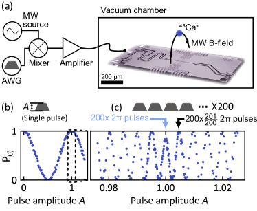
Figure 1: Non-linear drive chain and Rabi-oscillation distortion. (a) Overview of the experimental setup showing a simplified schematic of the MW drive chain delivering pulses to a ${}^{\text{43}}$Ca⁺ trapped-ion qubit. The potential nonlinearity of the MW components needs to be identified and compensated for. Ion height and MW field not to scale. (b) Delivering a single pulse of fixed duration, but varied amplitude $A$, enables the observation of Rabi-oscillations. Here $P_{\ket{0}}$ corresponds to the probability of measuring the initial state $\ket{0}$ after the pulse. The amplitude is normalized such that $A=1$ corresponds to a pulse driving a $2\pi$ rotation of the qubit. (c) When $N$ pulses are delivered, the initial qubit state is in principle recovered when the pulse amplitude is an integer multiple of $1/N$. Here this is verified for $N=200$, and surprisingly is not the case for $A=1$. This exceptional point corresponds to the case where $N\times\ 2\pi$ pulses are nominally delivered. As explained in Fig. 2, this is a signature of a phase-amplitude relation, stemming from the nonlinearity of MW components.

High-fidelity control of quantum systems is crucial to quantum computing, as it can drastically minimize the overhead associated with error correction [1]. In many platforms, quantum gates are driven by laser, radio-frequency or microwave pulses, where low error rates depend on the accurate control of signal amplitude and phase. Distortions induced by the chain of components generating and delivering this drive signal should therefore be identified and corrected. A common compensation technique is to use “pre-distortion” such that distortions produce the desired pulse [2]. This is used in NMR [3], EPR [4], Rydberg atoms [5], Bose-Einstein condensates [6], and superconducting circuits [7, 8, 9]. In trapped ions [10], pre-distortion has been used to compensate for thermal transients in microwave circuitry [11], or for compensating filtering in fast shuttling operations [12]. Successful pre-distortion relies however on an accurate model of the drive chain, part of which is, for trapped ions, under high vacuum, microscopic and possibly cooled cryogenically [13]. Using conventional tools such as network analyzers is therefore not always possible.

Here, we demonstrate how a trapped ion qubit can be used as a sensor to characterize the distortion of gate pulses [7, 8, 9, 14]. We present a scheme which coherently amplifies the amplitude-dependent phase change of a microwave field. Pre-distortion is shown to compensate this drive chain imperfection, leading to a three-fold reduction in single-qubit gate error, to attain state of the art performance benchmarked at $1.6(4)\times 10^{-6}$ error per Clifford gate. This method is not restricted to microwave-driven trapped ion qubits and is in principle applicable to any quantum computing platform.

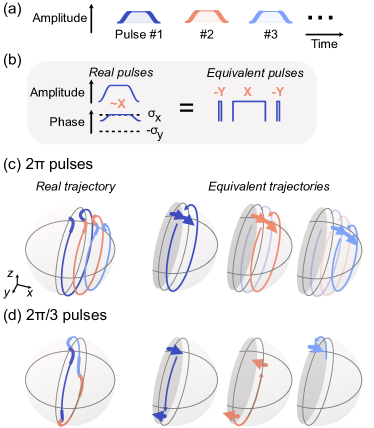
Figure 2: Coherent amplification of phase variations. (a) Schematic of the train of pulses applied to the qubit. These are intended to produce $x$-rotations. (b) If the MW phase depends on amplitude (“real pulses”), the resulting deviations in phase during ramp up/down can be described by a small $y$-rotation (“equivalent pulses”). The trajectory driven on the Bloch sphere by three successive pulses is shown in (c) and (d) for the real and equivalent pulses. The ramping or resulting $y$-rotations are shown in bold or with a thicker arrow. (c) In the case of a train of $2\pi$ pulses, since the qubit returns to the same part of the Bloch sphere for ramp-up/down of the pulse amplitude, the small $y$-rotations add up coherently, producing the exceptional $A=1$ point in Fig. 1(c). (d) Otherwise, for example here with $2\pi/3$ pulses, ramp-up/down occurs on varying parts of the Bloch sphere, such that the $y$-rotations cancel out, ensuring a return to the initial qubit state. To make the effect visible for just 3 pulses, ramp durations and phase deviations are exaggerated with respect to the experiment.

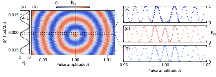
Figure 3: MW phase pre-distortion. Rabi-oscillations are measured as in Fig. 1(c) for a train of $N=200$ pulses. (a) For $A=1$, we vary the proportionality factor between phase and amplitude $\phi_{c}^{\prime}$, implemented in our AWG, whilst monitoring $P_{\ket{0}}$. Compensation of the effect is obtained for $\phi_{c}^{\prime}=-2\pi\times 1.8\times 10^{-3}$ radians. (b) $P_{\ket{0}}$ as a function of both $\phi_{c}^{\prime}$ and pulse amplitude $A$, where selected transects show that the effect can be accentuated (c, $\phi_{c}^{\prime}=2\pi\times 4.9\times 10^{-3}$) with respect to the case where the phase is not intentionally varied (d, $\phi_{c}^{\prime}=0$), or compensated for (e).

Experiments are carried out using a trapped ion qubit driven by near-field microwaves [15, 16, 11, 17, 18, 19]. Our qubit is defined by the hyperfine levels $\ket{0}=|F=3,M_{F}=1\rangle$ and $\ket{1}=|F=4,M_{F}=1\rangle$ of the ground state manifold 4S_1/2 of ⁴³Ca⁺, which form a clock transition at our static magnetic field strength of 28.8 mT. The ion is trapped $40\ \upmu$m above a surface “chip” trap, which features a microwave (MW) electrode used to drive the magnetic dipole moment of the qubit. Amplitude-shaped $\sim 100$ MHz pulses are generated using an arbitrary waveform generator (AWG), then up-converted using a $3$ GHz source and an IQ mixer to be brought into on resonance with the qubit frequency at 3.1 GHz. After amplification to $\sim$ 400 mW, the microwaves are delivered into the vacuum chamber to the surface trap where they drive the qubit. A simplified schematic of the experimental setup is shown in Fig. 1(a), with more detail in Sec. S2. Details on the trap and qubit state preparation and readout can be found in Ref [20].

These MW pulses, resonant with the qubit transition, will drive Rabi-oscillations, as shown in Fig. 1(b). Given our control system’s 1 ns timing resolution and our pulse duration of $1.2\ \upmu$s, varying the pulse amplitude at the AWG (with 15-bit resolution) offers a more precise method of tuning the pulse area than varying the pulse duration ($3\times 10^{-5}$ precision rather than $8\times 10^{-4}$). We therefore vary pulse amplitude rather than the more usual pulse time in these measurements. For a fixed pulse shape and duration, we define a pulse amplitude scaling factor $A$ such that $A=1$ produces a $2\pi$ rotation of the qubit. When $A$ is swept from 0 to 1, the probability $P_{\ket{0}}$ of recovering the initial qubit state $\ket{0}$ will undergo a single oscillation as shown in Fig. 1(a).

When driving the qubit with a train of $N$ (identical) pulses rather than one pulse, $P_{\ket{0}}$ should undergo $N$ oscillations rather than one in the same amplitude span. Indeed, at a pulse amplitude $A=n/N$, if $n$ is an integer, the cumulative effect of the pulse train should be to induce $n$ full rotations of the qubit state around the Bloch sphere. The resulting recovery to the initial state is observed in the measurement of Fig. 1(c), except for the case $A=1$, nominally corresponding to a train of $2\pi$ rotations.

To explain this phenomenon, we consider a change in MW phase $\phi(t)$ during the pulse, proportional to the pulse amplitude $a(t)$. We normalize $a$ such that $a(t)=A$ during the “plateau” of the pulse. The phase variation is assumed to be characterized by the phase-amplitude proportionality factor $\phi^{\prime}=\partial\phi/\partial a$, such that we have $\phi(t)=\phi^{\prime}a(t)+\phi_{0}$. We assume proportionality here, but higher order dependencies of phase on amplitude can be studied experimentally with an alternative scheme shown in Fig. S1. Such a phase-amplitude relation would come into play whilst ramping up/down the pulse, which is done in this experiment over a duration of $t_{\text{ramp}}=$200 ns per ramp (400 ns total ramping time over a pulse). This consideration is motivated by the number of potentially non-linear elements in the MW drive chain (AWG, mixer, amplifier). Without loss of generality, we set $\phi(t)=0$ during the “plateau” of the pulse such that the small phase variation perturbs the pulse – during the ramping – away from the ideal $x$-rotation. The resulting physics can be understood by constructing an equivalent unitary to that driven by the pulse train, where phase deviations manifest as small $y$-rotations at the beginning and end of each pulse train. This is schematically shown in Fig. 2(b) and formally derived in Sec. S1.1.

These small $y$-rotations will nearly always be inconsequential as the dominant $x$-rotation will dynamically decouple the qubit from non-commuting $y$-rotations. However, this is not the case at the exceptional $A=1$ point in Fig. 1(c), where the $x$-rotation is an identity operation, which then commutes with $y$-rotations. Indeed, at $A=1$, each pulse is approximately a $2\pi$ rotation around the $x$-axis, and ramping up/down the pulse always occurs when the qubit state is in the same area of the Bloch sphere. The $y$-rotations will then coherently add up such that, after $N=200$ pulses, the total $y$-rotation produces a noticeable decrease in $P_{\ket{0}}$. This is schematically shown in Fig. 2(c), with inflated ramping durations and phase variations such that the effect is noticeable after a few pulses. When pulses do not produce a $2\pi$ rotation, ramping up/down will occur at varying areas of the Bloch sphere as the train of pulses progresses, and the $y$-rotations tend to average out. This is illustrated in the case of $2\pi/3$ pulses in Fig. 2(d). As derived in Sec. S1.2, in the former case phase variations have a $\sim(N\phi^{\prime})^{2}$ impact on $P_{\ket{0}}$, whereas in the latter the effect is much smaller $\sim(N\phi^{\prime})^{4}$.

To verify this interpretation, we add a compensation phase proportional to the pulse amplitude $\phi_{c}(t)=a(t)\phi_{c}^{\prime}$ in the pulses generated by our AWG. This “pre-distorted” MW pulse then has a phase given by

$$\phi(t)=\phi_{n}(t)+\phi_{c}(t)=a(t)(\phi_{n}^{\prime}+\phi_{c}^{\prime})+\phi_{0}$$ (1)

where $\phi_{n}$ designates the phase variation native to the drive chain. Whilst varying the parameter $\phi_{c}^{\prime}$, we measure the distorted Rabi-oscillations to show that full contrast at $A=1$ can be recovered for $\phi_{c}^{\prime}=-2\pi\times 1.8\times 10^{-3}$ radians (Fig. 3). Here we are again using a train of 200 pulses just as in Fig. 1(c). This indicates that the phase does indeed change (linearly) with MW amplitude. A control experiment providing further confirmation of this fact is presented in Sec. S2.

Scanning both pulse amplitude $A$ and phase compensation $\phi_{c}^{\prime}$ whilst monitoring $P_{\ket{0}}$ reveals a symmetry in their influence (Fig. 3(b)). Indeed, whilst deviations of the pulse amplitude away from $A=1$ increases the amount of net rotation around the $x$-axis, increased phase variation during pulse ramping increases the accumulated $y$-rotation over the train of pulses. While a horizontal line-cut of Fig. 3 (Fig. 3(e)) describes Rabi-oscillations induced by $x$-rotations, a vertical line-cut (Fig. 3(a)) describes Rabi-oscillations induced by $y$-rotations. This is demonstrated more formally in Sec. S1.2 using perturbation theory, showing that for $|A-1|,|\phi(t)|\ll 1$, a train of $N$ pulses drives the unitary evolution

$$\hat{U}=\text{exp}\left(iN\Omega_{x}\hat{\sigma}_{x}+iN\Omega_{y}\hat{\sigma}_{y}\right)$$ (2)

with $\Omega_{x}\propto(A-1)$ and $\Omega_{y}\propto\phi^{\prime}$. This unitary results in the ring pattern observed in the measurement of Fig. 3(b):

$$P_{\ket{0}}=\frac{1}{2}\left(1+\cos\left(N\sqrt{\Omega_{x}^{2}+\Omega_{y}^{2}}\right)\right)\ .$$ (3)

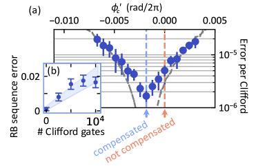
Figure 4: Application to high-fidelity quantum gates. (a) Dots are single-qubit gate errors measured using randomized benchmarking (RB) as a function of phase compensation. The error is reduced from $5(2)\times 10^{-6}$ to $1.6(4)\times 10^{-6}$ when using the phase compensation identified in Fig.3(a). The error scaling at higher phase compensation values is consistent with simulated RB data (gray dashed lines). Lower errors are limited by other physical mechanisms [19]. (b) RB sequence error as a function of the number of Clifford gates per sequence. Corresponds to lowest error where the phase variations are compensated for. The gate error is on par with state-of-the art errors across all quantum computing platforms [16, 19].

Whilst the phase change over a non-compensated pulse is small, it can be a leading source of error in the high-fidelity logic operations on trapped-ion qubits. Scanning the compensation parameter whilst monitoring $P_{\ket{0}}$ (Fig. 3(a)) constitutes a rapid calibration procedure sufficient to mitigate phase variations. To demonstrate this, we scan the phase compensation parameter $\phi_{c}^{\prime}$ whilst monitoring the single-qubit Clifford gate error with randomized benchmarking [21] (Fig. 4(a)). The error is reduced from $5(2)\times 10^{-6}$ to $1.6(4)\times 10^{-6}$ when using the phase compensation identified in Fig. 3(a). In this case, identifying and compensating for this small variation in phase brings single-qubit gate performance to state of the art error rates [19, 16].

We note that this problem is not present in previously reported error budgets [19] due to the different decomposition of Clifford gates into native MW pulses. Here, we decompose Clifford gates into $\pi$ and $\pi/2$ pulses, with the same pulse duration, but varying pulse amplitude. The bulk of the error arises here due to the $\times 2$ variation in pulse amplitude, which produces a change in the relative phases of $\pi$ and $\pi/2$ pulses. This error can thus also be mitigated by varying pulse times rather than amplitude or decomposing Clifford gates into only $\pi/2$ pulses. The latter was done in Ref. [19] after realizing the presence of this phase-amplitude relation. The residual error from phase variation during pulse ramping is then negligeable.

A calibration of phase variations is also useful in more complex composite pulse schemes. In particular when we want to leverage the fine pulse amplitude control from pulse to pulse – for example in the ion addressing scheme of Ref. [19]. In the addressing experiment, the combination of weak pulses (at least half the amplitude used in this work), and the dominance of drift-induced errors made the impact of phase variations negligeable. The average error over 100 different addressing pulse sequences is theoretically $9.0(2)\times 10^{-7}$, much smaller than the average error measured at $3.4\times 10^{-5}$. However, by simply doubling the amplitude and $\phi_{n}^{\prime}$, the error would have been considerable at $1.5(5)\times 10^{-5}$ per gate.

By measuring a scattering parameter ($S_{\text{21}}$) of the nonlinear components of our MW drive chain, we attempt to understand the native phase variation characterized by $\phi_{n}^{\prime}=2\pi\times 1.8\times 10^{-3}$ rad. Unfortunately, such measurements are limited to the phase precision of our vector network analyzer $\sim 2\pi\times 10^{-4}$ rad. The only component showing measurable phase variation is the amplifier with $\phi^{\prime}=2\pi\times 0.8\times 10^{-3}$, see measurement details in Sec. S2. In this experimental context, the Rabi-oscillation distortion is thus a much more sensitive method for diagnostic and compensation.

Finally, we note that the measurement scheme of Fig. 1(c) also enables the characterization of other drive chain distortions. If the Rabi-frequency scales linearly with the MW amplitude programmed in the AWG, then the period of oscillations in Fig. 1(c) should remain constant as the amplitude increases. In practice, we find that this is not the case, and this measurement constitutes a rapid calibration of this field-amplitude non-linearity which could be useful for e.g. the addressing scheme of Ref. [19].

In conclusion, we have presented a scheme to rapidly identify, and to compensate for, phase-amplitude relations in qubit drives. These phase variations are shown to be a dominant error in our implementation of microwave-driven quantum logic. Pre-distortion of the phase evolution during the pulse ramping is shown to be an effective mitigation technique. The resulting error rate, measured through randomized benchmarking ($1.6(4)\times 10^{-6}$ per Clifford gate), is consistent with the state of the art across all quantum computing platforms [16, 19]. The scheme is applicable to any qubit system driven by an amplitude-shaped pulse. Since the qubit itself is used to probe the field, it is particularly suited to systems partially inaccessible by more conventional sensors; systems under vacuum, cryogenic, or micro-/nano-meter in size.

Acknowledgments: This work was supported by the U.S. Army Research Office (ref. W911NF-18-1-0340) and the U.K. EPSRC Quantum Computing and Simulation Hub. M.F.G. acknowledges support from the Netherlands Organization for Scientific Research (NWO) through a Rubicon Grant. A.D.L. acknowledges support from Oxford Ionics Ltd.

Supplementary information

S1 Theory

S1.1 ZYXYZ decomposition

The Hamiltonian describing MW driving of the qubit with a time-varying phase writes

$$\hat{H}(t)=\hbar\underbrace{\Omega(t)\cos(\phi(t))}_{\Omega_{x}(t)}\hat{\sigma}_{x}/2+\hbar\underbrace{\Omega(t)\sin(\phi(t))}_{\Omega_{y}(t)}\hat{\sigma}_{y}/2\ ,$$ (S1)

in the interaction picture, where terms rotating at the qubit frequency have been neglected. Here $\hbar$ is the reduced Planck constant, $\hat{\sigma}_{x,y}$ are Pauli operators acting on the qubit states, and $\Omega(t),\phi(t)$ are the Rabi-frequency and phase of the drive. The variations in phase are assumed to arise from changes in amplitude, such that, without loss of generality, we can set $\phi(t)=0$ during the “plateau” of the pulse. The small phase variations then perturb the pulse – during the ramping – away from the ideal $x$-rotation. This Hamiltonian drives the following unitary evolution during ramping

$$\hat{U}_{\text{ramp}}=\exp[-i(r_{x}\hat{\sigma}_{x}+r_{y}\hat{\sigma}_{y})/2]\ ,$$ (S2)

where $r_{x,y}=\int_{0}^{t_{\text{ramp}}}\Omega_{x,y}(t)dt$. Upon ramp up, we decompose the unitary into $z$-, $y$- then $x$- rotation described by

$$\hat{U}_{\text{ramp}}\simeq\exp[-i\alpha_{x}\hat{\sigma}_{x}/2]\exp[-i\alpha_{y}\hat{\sigma}_{y}/2]\exp[-i\alpha_{z}\hat{\sigma}_{z}/2]\ ,$$ (S3)

where $\alpha_{x,y,z}$ are Tait-Bryan angles. Whilst the decomposition can be exact, we can assume small phase deviations $|\phi(t)|\ll 1$, implying $|r_{y}|\ll 1$, to simplify the expression for the rotation angles, given to first order by

$$\alpha_{x} =r_{x}$$ (S4)

$$\alpha_{y} =r_{y}\frac{\sin(r_{x})}{r_{x}}$$

$$\alpha_{z} =-r_{y}\frac{1-\cos(r_{x})}{r_{x}}\ .$$

Upon ramp-down, assuming a symmetric pulse $\int_{T-t_{\text{ramp}}}^{T}\Omega_{x,y}(t)dt=r_{x,y}$, we can decompose the unitary into a $x$-, $y$- then $z$- rotation described by

$$\hat{U}_{\text{ramp}}\simeq\exp[-i(-\alpha_{z})\hat{\sigma}_{z}/2]\exp[-i\alpha_{y}\hat{\sigma}_{y}/2]\exp[-i\alpha_{x}\hat{\sigma}_{x}/2]\ .$$ (S5)

The $z$-rotation angle has flipped sign here because of the change in the order of rotations with respect to the ramp-up. When constructing a train of pulses, the inter-pulse z-rotations of subsequent pulses cancel due to this sign flip. The remaining z-rotations at the beginning and end of the pulse train is negligeable, in addition to being irrelevant when preparing and measuring the qubit state in the computational basis. The $x$-rotations will dominate in the ramping portion of the pulse, and can be combined with the unitary describing the “plateau” portion of the pulse, resulting in the effective description of the pulse shown in Fig 2(a). Note that, given our definition of $\phi(t)$, and our assumption of positive proportionality factor between phase and amplitude in Fig. 2, $r_{y}<0$ in the trajectories of Fig. 2(b,c).

S1.2 Perturbation theory

To describe the data shown in Fig. 3(b), we the relation between amplitude and phase $\phi(t)=\phi^{\prime}(a(t)-A)$. The Hamiltonian introduced in Eq. (S1) then writes

$$\hat{H}(t)= \hbar\Omega a(t)\big{[}\cos\left(\phi^{\prime}\left(a(t)-A\right)\right)\hat{\sigma}_{x}/2$$ (S6)

$$+\sin\left(\phi^{\prime}\left(a(t)-A\right)\right)\hat{\sigma}_{y}/2\big{]}\ .$$

Here $a(t)$ describes the temporal profile and the amplitude of the pulse: we assume $\sin^{2}$ ramping over a duration $t_{\text{ramp}}$ at both the beginning and end of the pulse, and a plateau of amplitude $a(t)=A$. The quantity $\Omega=2\pi/(T-t_{\text{ramp}})$ can be seen as a normalization factor which ensures that

$$\int_{0}^{T}\Omega a(t)dt=2\pi A\ .$$ (S7)

We consider a small deviation $\epsilon$ from a pulse $a_{2\pi}$ generating $2\pi$ rotations in the absence of phase variations ($\int_{0}^{T}\Omega a_{2\pi}(t)dt=2\pi$), such that the pulse profile writes

$$a(t)=a_{2\pi}(t)(1+\epsilon)\ .$$ (S8)

In the limit $|\epsilon|,|\phi^{\prime}|\ll 1$, the parameter regime explored in Fig. 3(b), the Hamiltonian can be approximated as

$$\hat{H}(t) \simeq H_{0}(t)+H_{1}(t)\ ,$$ (S9)

$$\hat{H}_{0}(t) =\hbar\Omega a_{2\pi}(t)\hat{\sigma}_{x}/2\ ,$$

$$\hat{H}_{1}(t) =\hbar\Omega\left(\epsilon a_{2\pi}(t)\hat{\sigma}_{x}/2+\phi^{\prime}a_{2\pi}(t)(a_{2\pi}(t)-1)\hat{\sigma}_{y}/2\right)\ .$$

We aim to write the unitary evolution using first order perturbation theory:

$$\hat{U}(0,T) \simeq\hat{U}_{0}(0,T)+\hat{U}_{1}(0,T)\ ,$$ (S10)

$$\hat{U}_{0}(t_{0},t) =\exp\left[-\frac{i}{\hbar}\int_{t_{0}}^{t}\hat{H}_{0}(\tau)d\tau\right]$$

$$\hat{U}_{1}(0,T) =-\frac{i}{\hbar}\hat{U}_{0}(0,T)\int_{0}^{T}\hat{U}_{0}(t,0)\hat{H}_{1}(t)\hat{U}_{0}(0,t)dt\ .$$

Since textbooks tend to focus on the case where $H_{0}$ is time-independent, we have not been able to find a proof in the literature of this exact perturbative expansion of the unitary evolution operator. We therefore include a proof of (S10) in Sec. S1.3. The 0-th order term drives a rotation of angle $\theta(t)$ about the $x$- axis of the Bloch sphere:

$$\hat{U}_{0}(0,t) =\begin{pmatrix}\cos\left[\theta(t)/2\right]&-i\sin\left[\theta(t)/2\right]\\ -i\sin\left[\theta(t)/2\right]&\cos\left[\theta(t)/2\right]\\ \end{pmatrix},$$ (S11)

$$\hat{U}_{0}(t,0) =\begin{pmatrix}\cos\left[\theta(t)/2\right]&i\sin\left[\theta(t)/2\right]\\ i\sin\left[\theta(t)/2\right]&\cos\left[\theta(t)/2\right]\\ \end{pmatrix},$$

$$\theta(t) =\int_{0}^{t}\Omega a_{2\pi}(\tau)d\tau\ .$$

Here the definition of $a_{2\pi}$ means that $\theta(T)=2\pi$ and $\hat{U}_{0}(0,T)=-\mathds{1}$. Expressing $\hat{U}_{0}$ in this form is helpful when computing the first order term

$$\hat{U}_{1}(0,T) =i\epsilon A_{x}\hat{\sigma}_{x}/2+i\phi^{\prime}A_{y}\hat{\sigma}_{y}/2\ ,$$ (S12)

$$A_{x} =\int_{0}^{T}\Omega a_{2\pi}(t)dt=2\pi\ ,$$

$$A_{y} =\int_{0}^{T}\Omega a_{2\pi}(t)(a_{2\pi}(t)-1)\cos(\theta(t))dt\ .$$

To derive this expression, we have relied on the fact that $\int_{0}^{T}\sin(\theta(t))a(t)(a_{2\pi}(t)-1)=0$ since $\sin(\theta(t))$ and $a(t)$ are antisymmetric and symmetric respectively about $t=T/2$. The total unitary in first order perturbation theory is then (up to a global phase)

$$\hat{U}(0,T) \simeq\mathds{1}-i\epsilon A_{x}\hat{\sigma}_{x}/2-i\phi^{\prime}A_{y}\hat{\sigma}_{y}/2$$ (S13)

$$\simeq\exp\left[-i\epsilon A_{x}\hat{\sigma}_{x}/2-i\phi^{\prime}A_{y}\hat{\sigma}_{y}/2\right]$$

where the exponential form is equivalent to first order in $\epsilon,\phi^{\prime}$. The exponential form makes the cumulative effect of multiple pulses easier to calculate:

$$\hat{U}(0,T)^{N}\simeq\exp\left[-iN\left(\epsilon A_{x}\hat{\sigma}_{x}/2+\phi^{\prime}A_{y}\hat{\sigma}_{y}/2\right)\right]\ .$$ (S14)

This unitary corresponds to Rabi-oscillations with effective Rabi-frequency $N\sqrt{(\epsilon A_{x})^{2}+(\phi^{\prime}A_{y})^{2}}$ and the probability of recovering the initial qubit state $\ket{0}$ is

$$P_{\ket{0}}=\frac{1}{2}\left(1+\cos\left(N\sqrt{(\epsilon A_{x})^{2}+(\phi^{\prime}A_{y})^{2}}\right)\right)\ .$$ (S15)

Plotting $P_{\ket{0}}$ reproduces the concentric circles of Fig. 3(b) where $\epsilon$ and $\phi^{\prime}$ are varied in the $x$ and $y$ axes respectively.

At $\epsilon=0$ ($A=1$), the probability $P_{\ket{0}}$ is approximately

$$P_{\ket{0}}\simeq 1-\frac{1}{2}\left(N\phi^{\prime}A_{y}\right)^{2}\ ,$$ (S16)

showing a quadratic dependence on phase variations. In the regime where $x$-rotations dominate instead ($|\epsilon A_{x}|\gg|\phi^{\prime}A_{y}|$) – for example at a pulse amplitude $\epsilon=1/N$ ($A=(N+1)/N$) which shows full contrast in Figs. 1,3 – we have

$$P_{\ket{0}}\simeq 1-\frac{1}{32\pi^{2}}\left(N\phi^{\prime}A_{y}\right)^{4}\ .$$ (S17)

showing a much smaller quartic dependence on phase variations. Given the temporal profile of our pulse, and in the absence of any compensation for phase variations, the transition point between these two regimes ($|\epsilon A_{x}|=|\phi^{\prime}A_{y}|$) occurs for $|\epsilon|=1\times 10^{-3}$, which is much smaller than the period of oscillations $1/N=5\times 10^{-3}$ shown in Figs. 1,3. This explains why loss of contrast only occurs around $A=1$.

S1.3 Perturbative expansion of $\hat{U}$

Here we provide proof of the perturbative expansion introduced in Eq. (S10). We consider a more generic Hamiltonian

$$\hat{H}(t)=\hat{H}_{0}(t)+\eta\hat{H}_{1}(t)\ .$$ (S18)

We want to write a perturbative expansion for the unitary evolution operator $\hat{U}(t_{0},t)$ under the assumption $\eta\ll 1$:

$$\hat{U}(t_{0},t)=\hat{U}_{0}(t_{0},t)+\eta\hat{U}_{1}(t_{0},t)+\eta^{2}\hat{U}_{2}(t_{0},t)+...\ .$$ (S19)

The operator $\hat{U}$ follows

$$\hat{H}(t)\hat{U}(t_{0},t)\psi(t_{0})=i\hbar\frac{\partial}{\partial t}\hat{U}(t_{0},t)\psi(t_{0})$$ (S20)

and substituting $\hat{H},\hat{U}$ from Eqs (S18,S19) for $\eta=0$ yields the equation defining the 0-th order term

$$\hat{H}_{0}(t)\hat{U}_{0}(t_{0},t)\psi(t_{0})=i\hbar\frac{\partial}{\partial t}\hat{U}_{0}(t_{0},t)\psi(t_{0})$$ (S21)

which we integrate to obtain

$$\hat{U}_{0}(t_{0},t)=\exp\left[-\frac{i}{\hbar}\int_{t_{0}}^{t}\hat{H}_{0}(\tau)d\tau\right]\ .$$ (S22)

We now write the first-order equation by injecting $\hat{H},\hat{U}$ from Eqs. (S18,S19) into Eq. (S20), neglecting terms in $\eta^{n},n>1$, and making use of Eq. (S21) to obtain

$$\left(\hat{H}_{1}(t)\hat{U}_{0}(t_{0},t)+\hat{H}_{0}(t)\hat{U}_{1}(t_{0},t)\right)\psi(t_{0})=i\hbar\frac{\partial}{\partial t}\hat{U}_{1}(t_{0},t)\psi(t_{0})\ ,$$ (S23)

providing the first order contribution

$$\hat{U}_{1}(t_{0},t)=-\frac{i}{\hbar}\hat{U}_{0}(t_{0},t)\int_{t_{0}}^{t}U_{0}(\tau,t_{0})\hat{H}_{1}(\tau)\hat{U}_{0}(t_{0},\tau)d\tau\ .$$ (S24)

Injecting this expression for $\hat{U}_{1}(t_{0},t)$ in Eq (S23), and utilizing the fact that $\hat{U}_{0}(t_{0},t)\hat{U}_{0}(t,t_{0})=\mathds{1}$ demonstrates the validity of Eq. (S24).

S2 Supporting measurements

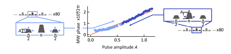
Figure S1: Alternative measurement of the phase-amplitude relation. A train of 80 $\pi/2-\pi-\pi/2$ pulse sequences is delivered to the qubit. In the absence of phase variations between the pulses, the sequence should have no net effect on the qubit. If a phase-amplitude relation exists however, maintaining a large difference in amplitude between the $\pi/2$ and $\pi$ pulses leads to phase differences between these two pulses. The pulse sequence then induces a change in the qubit state, which coherently adds up with the number of sequences, from which the phase difference can be inferred.
We vary the amplitude and duration of the $\pi$ or $\pi/2$ pulses, maintaining an approximately constant pulse area, to map out the phase-amplitude relationship. The measurement has to be carried out in two steps however, if the full range of microwave amplitudes is to be explored. Indeed, the sensitivity of this measurement increases with the difference in amplitude between the pulses. In the light blue data, we start with the shortest, highest amplitude $\pi$ pulse possible, and increase the $\pi/2$ amplitude until phase variations are difficult to resolve. In the dark blue data, we start with $A\sim 0$ amplitude $\pi/2$ pulse, and decrease the amplitude of $\pi$ pulses until sensitivity is lost.
Maintaining the correct pulse area is complicated by the lack of control over pulse time (relative to the high degree of control over amplitude), as well as amplitude non-linearity (the amplitude requested from the AWG is not proportional to the field amplitude at the ion). In practice, we find that a slight adjustment of the amplitude of one of the pulses is required for each point shown in this figure. Each measurement (light/dark blue points) are thus extracted from different 2-dimensional parameter scans, which are considerably longer to carry out than the calibration demonstrated in Fig. 3(a). This measurement does, however, demonstrate an approximately linear phase-amplitude relationship, confirming the findings reported in the main text.

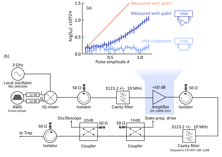
Figure S2: Nonlinearity in the microwave amplifier (a) The measured phase shift induced by the amplifier (Arg[$S_{\text{21}}$]) used in the qubit microwave drive chain is shown in dark blue. The measurement is carried out using a vector network analyzer (Rohde&Schwarz ZVL) with a precision of $~{}2\pi 10^{-4}$ radians, measured in the control experiment shown in light blue where the amplifier is removed from the measured network. The amplifier contributes to $\phi^{\prime}=2\pi\times 0.8\times 10^{-3}$ of the total phase shift $\phi^{\prime}=2\pi\times 1.8\times 10^{-3}$ measured using the qubit (orange). (b) Microwave setup used to drive the qubit, showing the multitude of potentially nonlinear components which could produce phase shifts. The AWG, IQ-mixer and amplifier were probed for such an effect, but only the amplifier showed a phase variation exceeding the precision of the VNA measurement.

References

- Knill [2010] E. Knill, Quantum computing, Nature 463, 441 (2010).
- Hincks et al. [2015] I. N. Hincks, C. E. Granade, T. W. Borneman, and D. G. Cory, Controlling quantum devices with nonlinear hardware, Phys. Rev. Appl. 4, 024012 (2015).
- Tabuchi et al. [2010] Y. Tabuchi, M. Negoro, K. Takeda, and M. Kitagawa, Total compensation of pulse transients inside a resonator, Journal of Magnetic Resonance 204, 327 (2010).
- Spindler et al. [2017] P. E. Spindler, P. Schöps, W. Kallies, S. J. Glaser, and T. F. Prisner, Perspectives of shaped pulses for epr spectroscopy, Journal of Magnetic Resonance 280, 30 (2017), special Issue on Methodological advances in EPR spectroscopy and imaging.
- Singh et al. [2023] J. Singh, R. Zeier, T. Calarco, and F. Motzoi, Compensating for nonlinear distortions in controlled quantum systems, Phys. Rev. Appl. 19, 064067 (2023).
- Jäger and Hohenester [2013] G. Jäger and U. Hohenester, Optimal quantum control of bose-einstein condensates in magnetic microtraps: Consideration of filter effects, Phys. Rev. A 88, 035601 (2013).
- Gustavsson et al. [2013] S. Gustavsson, O. Zwier, J. Bylander, F. Yan, F. Yoshihara, Y. Nakamura, T. P. Orlando, and W. D. Oliver, Improving quantum gate fidelities by using a qubit to measure microwave pulse distortions, Phys. Rev. Lett. 110, 040502 (2013).
- Jerger et al. [2019] M. Jerger, A. Kulikov, Z. Vasselin, and A. Fedorov, In situ characterization of qubit control lines: A qubit as a vector network analyzer, Phys. Rev. Lett. 123, 150501 (2019).
- Lazăr et al. [2023] S. Lazăr, Q. Ficheux, J. Herrmann, A. Remm, N. Lacroix, C. Hellings, F. Swiadek, D. C. Zanuz, G. J. Norris, M. B. Panah, A. Flasby, M. Kerschbaum, J.-C. Besse, C. Eichler, and A. Wallraff, Calibration of drive nonlinearity for arbitrary-angle single-qubit gates using error amplification, Phys. Rev. Appl. 20, 024036 (2023).
- Bruzewicz et al. [2019] C. D. Bruzewicz, J. Chiaverini, R. McConnell, and J. M. Sage, Trapped-ion quantum computing: Progress and challenges, Applied Physics Reviews 6 (2019).
- Harty et al. [2016] T. P. Harty, M. A. Sepiol, D. T. C. Allcock, C. J. Ballance, J. E. Tarlton, and D. M. Lucas, High-fidelity trapped-ion quantum logic using near-field microwaves, Phys. Rev. Lett. 117, 140501 (2016).
- Bowler et al. [2013] R. Bowler, U. Warring, J. W. Britton, B. C. Sawyer, and J. Amini, Arbitrary waveform generator for quantum information processing with trapped ions, Review of Scientific Instruments 84, 033108 (2013).
- Poitzsch et al. [1996] M. E. Poitzsch, J. C. Bergquist, W. M. Itano, and D. J. Wineland, Cryogenic linear ion trap for accurate spectroscopy, Review of Scientific Instruments 67, 129 (1996).
- Kristen et al. [2020] M. Kristen, A. Schneider, A. Stehli, T. Wolz, S. Danilin, H. S. Ku, J. Long, X. Wu, R. Lake, D. P. Pappas, et al., Amplitude and frequency sensing of microwave fields with a superconducting transmon qudit, npj Quantum Information 6, 57 (2020).
- Ospelkaus et al. [2008] C. Ospelkaus, C. E. Langer, J. M. Amini, K. R. Brown, D. Leibfried, and D. J. Wineland, Trapped-ion quantum logic gates based on oscillating magnetic fields, Phys. Rev. Lett. 101, 090502 (2008).
- Harty et al. [2014] T. P. Harty, D. T. C. Allcock, C. J. Ballance, L. Guidoni, H. A. Janacek, N. M. Linke, D. N. Stacey, and D. M. Lucas, High-fidelity preparation, gates, memory, and readout of a trapped-ion quantum bit, Phys. Rev. Lett. 113, 220501 (2014).
- Zarantonello et al. [2019] G. Zarantonello, H. Hahn, J. Morgner, M. Schulte, A. Bautista-Salvador, R. F. Werner, K. Hammerer, and C. Ospelkaus, Robust and resource-efficient microwave near-field entangling gate, Phys. Rev. Lett. 123, 260503 (2019).
- Srinivas et al. [2021] R. Srinivas, S. C. Burd, H. M. Knaack, R. T. Sutherland, A. Kwiatkowski, S. Glancy, E. Knill, D. J. Wineland, D. Leibfried, A. C. Wilson, D. T. C. Allcock, and D. H. Slichter, High-fidelity laser-free universal control of trapped ion qubits, Nature 597, 209–213 (2021).
- Leu et al. [2023] A. D. Leu, M. F. Gely, M. A. Weber, M. C. Smith, D. P. Nadlinger, and D. M. Lucas, Fast, high-fidelity addressed single-qubit gates using efficient composite pulse sequences, Phys. Rev. Lett. 131, 120601 (2023).
- Weber et al. [2022] M. A. Weber, C. Löschnauer, J. Wolf, M. F. Gely, R. K. Hanley, J. F. Goodwin, C. J. Ballance, T. P. Harty, and D. M. Lucas, Cryogenic ion trap system for high-fidelity near-field microwave-driven quantum logic (2022), arXiv:2207.11364 [quant-ph] .
- Knill et al. [2008] E. Knill, D. Leibfried, R. Reichle, J. Britton, R. B. Blakestad, J. D. Jost, C. Langer, R. Ozeri, S. Seidelin, and D. J. Wineland, Randomized benchmarking of quantum gates, Phys. Rev. A 77, 012307 (2008).