DriveSceneGen: Generating Diverse and Realistic Driving Scenarios from Scratch

Abstract

Realistic and diverse traffic scenarios in large quantities are crucial for the development and validation of autonomous driving systems. However, owing to numerous difficulties in the data collection process and the reliance on intensive annotations, real-world datasets lack sufficient quantity and diversity to support the increasing demand for data. This work introduces DriveSceneGen, a data-driven driving scenario generation method that learns from the real-world driving dataset and generates entire dynamic driving scenarios from scratch. DriveSceneGen is able to generate novel driving scenarios that align with real-world data distributions with high fidelity and diversity. Experimental results on 5k generated scenarios highlight the generation quality, diversity, and scalability compared to real-world datasets. To the best of our knowledge, DriveSceneGen is the first method that generates novel driving scenarios involving both static map elements and dynamic traffic participants from scratch.

I INTRODUCTION

In recent years, data-driven approaches have garnered increasing popularity in the autonomous driving research community. Many of the latest achievements in this field are powered by deep learning models trained on large amounts of data collected from real-world driving scenarios. For this class of methods, having large amounts of different scenarios is paramount for their performance and generalization capability. Particularly for the decision-making and planning modules in autonomous systems, it is important to ensure safety and sufficient capability to handle challenging scenarios by training and validating the system on a wide variety of driving scenarios. For this reason, the demand for more driving scenarios has been rapidly growing over the years. As part of this endeavor, numerous research institutions and autonomous vehicle companies have released a range of public driving datasets[1, 2, 3, 4]. However, despite the fact that these are real-world datasets collected from various locations covering a large number of scenarios, several notable limitations still persist.

Limited quantity and variety. In terms of data quantity, most existing datasets only contain about 300 to 500 hours, 290 to 1750 km of driving data. In comparison, an average American driver drives 21,688 km annually [5]. The data quantity is still not satisfactory compared to human statistics. In terms of data diversity, most datasets were only collected in a few US cities, limited by the available testing areas. Within each dataset, the number of unique scenes, i.e., geo-locations with distinct map typologies, is also limited, further constraining the generalizability of the dataset.

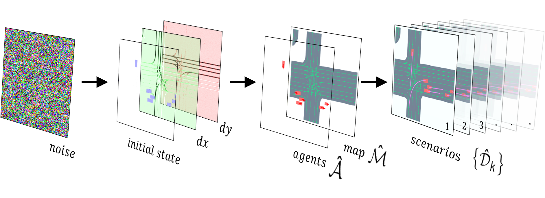
Figure 1: An illustration of a set of generated scenarios and its components at the various stages of DriveSceneGen pipeline.

Non-deterministic nature of agents’ driving behaviors. It is worth noting that the joint distribution of all traffic participants’ behaviors is inherently non-deterministic. Starting from the same initial scene, an unlimited number of possible futures could unfold. At every time step, each traffic participant receives new partial observations and makes individual judgments upon every smallest nuance occurring in the scene, resulting in drastically different driving scenarios in the end. However, real-world datasets could only capture the one that was developed at the time of collection, which can cause a significant loss of data diversity.

Expensive and Time-consuming. One of the major limitations of real-world datasets is that the collection process requires specialized equipment and licensing, often making the acquisition process extremely expensive. The post-processing and labeling of the collected scenario data also tend to be labor-intensive and time-costly, further limiting the availability of data to most researchers and institutes.

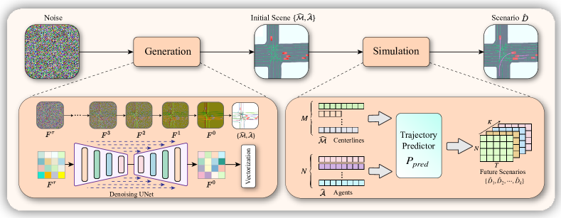
Figure 2: An overview of the DriveSceneGen pipeline. The pipeline consists of two stages: a generation stage and a simulation stage. In the generation stage, a diffusion model is employed to generate a rasterized Birds-Eye-View (BEV) representation of the initial scene of the driving scenario, which is then decoded by a rule-based vectorization method. In the simulation stage, the vectorized representation of the scenario is consumed by a simulation network as the initial scene to predict multi-modal joint distributions of the generated agents’ future trajectories, with each distribution representing a distinct possible outcome from this same initial scene.

Motivation and Contributions. With the understanding of these limitations of existing real-world datasets and the rising need for more data, we wish to leverage the latest generative models to learn the real-world distribution of various driving scenarios and then generate novel scenarios from this learned distribution. The contributions of this paper can summarized in fourfold:

• We propose the first method for generating novel driving scenarios from scratch, including both static lane maps and dynamic traffic agents, following a generation-simulation two-stage pipeline.

• We introduced a diffusion model in the generation stage of our method to generate a realistic birds-eye-view (BEV) feature map of the scenario, detailing both static map elements and dynamic agents’ initial states, which are then converted to its vectorized data form by a rule-based vectorization method.

• We repurposed a trajectory prediction model in the simulation stage to predict the multi-modal behaviors of each agent and form multiple joint predictions as different possible future scenarios, conditioned on the generated map and agents’ initial states.

• Experimental evaluations on the 5$k$ scenarios generated by our proposed method demonstrate that our method is able to achieve high fidelity and diversity compared to the 70k ground truth scenarios.

II RELATED WORKS

II-A Diffusion models

Denoising Diffusion Probabilistic Models (DDPM))[6, 7], often simply referred to as diffusion models, is a new class of generative models. These models demonstrate high generation-quality in image-related tasks such as image generation[8], inpainting[9], denoising, etc. At the same time, diffusion models have also gained success in a wide range of other domains, including sequence generation[10, 11], decision-making, planning[12, 13] and character animation[14]. Experimental evidence also showed that training with synthetic data generated by diffusion models can improve task performance on tasks such as image classification[15]. Building on prior works that demonstrated the model’s ability to produce high-quality samples in various domains, we are the first to apply diffusion models for the generation of autonomous driving datasets.

II-B Simulation Networks and Map Generation

A typical driving scenario mainly consists of two layers of information: a static map layer detailing the lanelet network and a dynamic agent layer that records the traffic agents and their corresponding driving trajectories. Many previous works have attempted to generate diverse agent trajectories based on a given real map. Works including [16, 17, 18] focused on sampling agent states from existing scenarios, then erasing and respawning the agents based on agent state distribution. Trafficgen[18] encoded both lane and agent data into a graph structure and summarized agent states using a Gaussian Mixture Model (GMM) and employing a Multi-Layer Perceptron (MLP) to model and simulate the distribution of agent states. SimNet[17] constructed the dynamic state of agents as a Markov Process and further learned both the state distribution and transition function using a Neural Network. However, these methods are only able to generate dynamic agents with a reliance on a given static map as the condition.

One existing work that attempted static map generation is HDMapGen[19], which autoregressively generated static lane structures as hierarchical graphs. However, the local details of the generated maps are not sufficiently realistic. And the model is not capable of generating complex and diverse road networks, limiting its practical applications.

To bridge the gap in the existing research between static map generation and dynamic agent simulation, we propose an entire driving scenario generation technique that includes static and dynamic elements, enhancing the diversity of scenarios and maintaining the consistency between static maps and dynamic agents.

III METHODOLOGY

III-A Overview of the Proposed Method

The proposed method mainly consists of two stages: a generation stage and a simulation stage, as shown in Fig. 2. First, in the generation stage, a diffusion model is employed to generate a rasterized Birds-Eye-View (BEV) representation of the initial scene of the driving scenario, which is then decoded by a rule-based vectorization method. Second, in the simulation stage, the vectorized representation of the scenario is consumed by a simulation network as the initial scene to predict multi-modal joint distributions of the generated agents’ future trajectories, with each distribution representing a distinct possible outcome from this same initial scene.

III-B Generation

A Diffusion Model for Driving Scenarios. A typical driving scenario $D$ can be divided into two major components: a static map layer $\mathcal{M}$ detailing the lanelet network and a dynamic agent layer $\mathcal{A}$ that records a set of traffic agents and their corresponding driving trajectories. The map $\mathcal{M}$ consists of a set of lanelets (or lanes), where each lanelet can be described by an imaginary polyline $\mathcal{P}$ as its centerline, which is essentially a set of waypoints $p\in\mathbb{R}^{2}$ connected according to the driving direction. Over the entire scenario time span $T$, the map information is assumed to be invariant, while each agent $A_{i}\in\mathcal{A}$ is updated at every time step $t$. An agent’s states over this time span can be represented by a bounding box $b\in\mathbb{R}^{2}$ containing the length and width of the vehicle, and a trajectory $\pi$, which consists of a set of vehicle states $\{s_{t}\mid 0\leq t\leq T\}$. Each state $s_{t}=[x,y,\theta,v]^{T}$ is a vector describing the vehicle x, y coordinates, heading, and velocity at time step $t$.

For the generation task, we define a rasterization function $f\colon D(\mathcal{M},\mathcal{A})\rightarrow F$, which encodes the above-mentioned map and agent data of a single driving scenario within a local region of $R$ meters into one rasterized BEV feature map $F\in\mathbb{R}^{W\times H\times C}$, where $W$ and $H$ denote the image width and height, and $C$ denotes the channels. At each coordinate location $(x,y)$, the value $C_{x,y}^{i}$ at each channel $i$ is used to encode a different type of information.

We propose an encoding strategy that augments the current centerlines with explicit directional information to help the model better learn the topological connection among them. For each waypoint $p=[x,y]^{T}$ on the centerline, we append an additional directional vector $\Delta p=[dx,dy]^{T}$, which points from waypoint $p_{i}$ to $p_{i+1}$, to the existing coordinate vector. Then, the centerlines are represented in the feature map with the $dx,dy$ encoded as values at two channels, respectively:

$$[C_{x,y}^{1},C_{x,y}^{2}]^{T}=0.5\times\left(1+\frac{\Delta p}{\|\Delta p\|_{2}}\right)\\$$ (1)

The directional vectors are assumed to be $[0,0]^{T}$ for non-lane areas. For each scenario, a transform $\mathbf{T}\colon(x,y)\rightarrow(i,j)$ is computed to map all real-world coordinates into a pixel location on the feature map.

Meanwhile, each agent’s initial state is represented by a rectangle bounding box $bbox$ according to its position and heading on the third channel of the feature map $C_{x,y}^{3}$, with the values within the bounding box region representing the vehicle’s velocity. A background value is assigned for regions in the feature map not occupied by any agent instead.

$$C_{x,y}^{3}=\left\{\begin{array}[]{cl}0.5\times\left(1+k_{v}*v\right)&\quad\textrm{if }(x,y)\subseteq bbox\\ 0&\quad\textrm{otherwise}\end{array}\right.$$ (2)

With each driving scenario $D_{i}$ being encoded into a rasterized format $F_{i}$ with the strategies described above, a diffusion model $\Theta$ is employed to learn a distribution $P(\mathcal{D})$ of the real-world driving scenarios from dataset $\mathcal{D}=\{F_{1},F_{2},\dots,F_{N}\}$. Subsequently, new driving scenarios $\hat{F}$ can be sampled from this learned distribution: $\hat{F}\sim P(\mathcal{D}|\Theta)$ as our desired outputs.

For this task, a DDPM model[7], with a U-Net[20] structure as its backbone, is designed to predict the noise added at each diffusion step. The U-Net comprises four down and up blocks, and a middle block. Each down block and up block consists of two ResNet blocks, while the middle block is made up of a self-attention layer and two ResNet blocks.

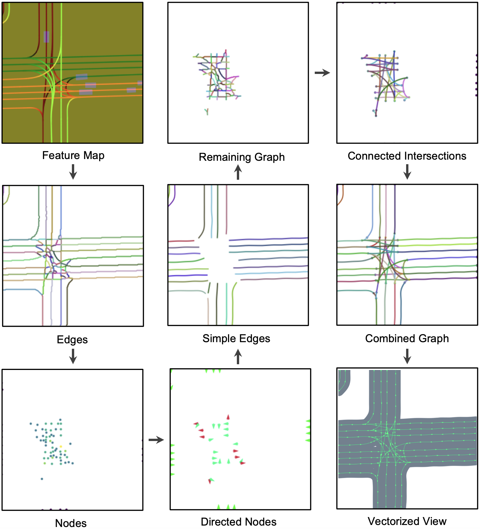
Figure 3: A visualization of the results obtained at each stage of the proposed vectorization method. The example feature map used represents a scene of 80$m\ \times$ 80$m$.

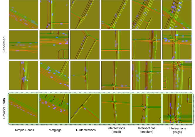
Figure 4: Qualitative evaluation of the raster initial scenes generated by DriveSceneGen. Compared to the ground truths, the generated samples show high fidelity in terms of road geometry, lane topology, and agents’ initial state distribution. Meanwhile, the generated results demonstrate both inter-category and intra-category diversities.

Vectorization. Once the diffusion model generates a new scenario sample, a vectorization process is applied to decode the scenario information from the feature map representation to its vector form $f^{-1}\colon\hat{F}\rightarrow\hat{D}$. It is worth highlighting that, in some applications, the generated scenarios in their current form can be directly used by methods that use raster data as inputs. However, for a more general purpose of use, we explicitly reconstruct the vectorized data $\hat{D}$ from the feature map $\hat{F}$.

To achieve this, we propose a graph-based method that extracts lane geometries from the generated feature map and recovers their topological connections, as illustrated in Fig. 3. First, the colored line features are extracted from the original feature map as edges $\mathcal{E}$, and the locations where multiple lines intersect are detected as vertices $\mathcal{V}$, using the method described in [21]. Then, an undirected graph can be established as $G\{\mathcal{V},\mathcal{E}\}$. Next, the directional vectors at each vertex location can be recovered by inverting Eq. 1. Among all the vertices, we are particularly interested in the vertices with a degree of 1 (terminal vertex $V_{i}^{t}$) and their corresponding neighbors (branching vertex $V_{i}^{b}$). With their directions computed, these special vertices can be simply labeled into two types: entry or exit, as shown in green and red colors in Fig.3. The assigned vertex type represents if an agent enters or exits an intersection along the driving direction. For each edge $E(V_{i}^{t},V_{i}^{b})$ that connects a terminal vertex $V_{i}^{t}$ and its branching vertex $V_{i}^{b}$, a directed edge can be extracted from graph $G$ into a new directed graph $G_{dir}$, following the driving direction. In the remaining graph, only intersection regions are present, including all branching vertices $\mathcal{V}^{b}$ with their labels, along with all the rest of the unclassified vertices. At this stage, for every pair of entry and exit vertices in the remaining graph $(V_{i}^{in},V_{j}^{out})$, a bézier curve is fitted to connect them if there exists a path between the two vertices. If the geometric of the fitted curve satisfies a set of rules, a new directed edge $E_{dir}(V_{i}^{in},V_{j}^{out})$ is added to the directed graph $G_{dir}$. Finally, the extracted simple edges and the fitted edges at intersections are combined and converted to a set of polylines $\mathcal{P}$ to form the final vectorized map $\mathcal{\hat{M}}$.

III-C Simulation

The aim of the simulation stage is to generate a set of potential future trajectories $\hat{\Pi}_{i}$ for each generated agent $\hat{A}_{i},i=\{1,\dots,N\}$ conditioned on the generated map context $\hat{\mathcal{M}}$ as well as the generated agents information $\hat{\mathcal{A}}$. A single future trajectory $\hat{\pi}_{i}$ belonging to a generated agent $\hat{A}_{i}$ can be represented as a sequence of states $\hat{s}_{i}^{t}$ at discrete time steps $t=\{1,\dots,T\}$ within the time horizon $T$. For each generated initial agent state $\hat{A}_{i}^{0}$, we wish to predict $K$ number of possible future candidate trajectories $\hat{\pi}_{i,k},k=\{1,\dots,K\}$, as well as their probability $p_{i,k}$. With the simulation model $P_{sim}$, the simulation problem can be mathematically expressed as $\{\hat{\pi}_{i,k}^{1:T},p_{k}\}_{\begin{subarray}{c}i\in\{1,\dots,N\},k\in\{1,\dots,K\}\end{subarray}}=\mathcal{P}_{sim}\left(\hat{\mathcal{M}},\{\hat{A}_{1}^{0},\dots,\hat{A}_{N}^{0}\}\right)$. By observing the problem defined above, this conditional generation problem can be treated as a relaxed form of the trajectory prediction problem, which aims to predict the same set of future trajectories conditioned on agents’ initial states with additional historical information over $\{-T_{h},\dots,0\}$ time steps: $\mathcal{P}_{pred}\left(\hat{\mathcal{M}},\{\hat{A}_{1}^{-T_{h}:0},\dots,\hat{A}_{N}^{-T_{h}:0}\}\right)$. Thus, generic trajectory prediction methods can be employed in the simulation stage as the backbone. To demonstrate the usability of our generated data, we leverage the recent developments in the trajectory prediction field and repurposed an MTR[22] model, which shows state-of-the-art multi-modal performance. The inputs to the model are configured to be the generated lane centerlines $\hat{\mathcal{M}}=\{\hat{\mathcal{P}_{1}},\dots,\hat{\mathcal{P}_{M}}\}$ and agents’ initial states $\hat{\mathcal{A}}=\{\hat{A}_{1}^{0},\dots,\hat{A}_{N}^{0}\}$. From the same initial scene, the model’s top $K$ marginal predictions $\{\hat{\pi}_{i,k}^{1:T},p_{k}\}$ are joined to form $K$ joint predictions $\{\hat{\Pi}_{k}\mid k={1,\dots,K}\}$, with each representing a distinct potential future scenario $\hat{D}_{k}$.

TABLE I: Generation Fidelity & Diversity

	Range ($m$)	Channels			FID $\downarrow$	Diversity
		1	2	3		Generated	Groundtruth	Discrepency % $\downarrow$
Map only	80	centerlines	centerlines	centerlines	206.49	15.25	17.27	11.69
		dx	dy	gray	35.75	17.37	17.76	2.19
Map + Agent		dx	dy	trajectories	90.56	17.84	18.44	3.25
		dx	dy	initial states	46.81	18.18	18.41	1.25
	120	dx	dy	initial states	44.69	17.64	18.11	2.59
	160	dx	dy	initial states	46.40	17.63	17.91	1.56

IV EXPERIMENTS

IV-A Experiment Setup

We evaluate the performance of DriveSceneGen on the Waymo Motion dataset [1], which contains 70k driving scenarios of 20 seconds duration. Unless specified, all models are trained at a resolution of $256\,\times 256\,$ on 4 NVIDIA V100 GPUs with a total batch size of 36 for 50 epochs. The training timesteps are set to 1000, and the AdamW optimizer is utilized with a learning rate of 1e-5. The number of model parameters for each is 56M.

IV-B Generation Fidelity & Diversity

Baselines. To assess the variations in different generation methods, we explored two generation modes: one designed for scenarios featuring only static maps, and another for scenarios that combine both static maps and dynamic agents. For the map-only generation mode, two encoding strategies are explored: (1), which encodes plain centerlines into three feature map channels without the directional vector information, and (2), which encodes $dx$, $dy$ in the first two channels of the scenario with the third channel filled with $0.5$. For the map + agent generation mode, we designed two different encoding strategies: (3), which encodes the agents as a set of trajectories, and (4), which encodes the agents as a set of initial states.

Quantitative Evaluation. Two commonly used metrics are adopted to evaluate the quality of the generated initial scenes. To measure the fidelity, Fréchet Inception Distance (FID) [23] is used to compute the distance between the feature vectors of the 5$k$ generated initial scenes and the feature vectors of the 70$k$ initial scenes in the ground truth dataset, both extracted by the Inception V3 network. A lower FID score indicates a higher generation fidelity. To measure the diversity, the average feature distance [24] among the feature vectors of the 5$k$ samples generated by each method is computed and compared with that of the 70$k$ ground truths in the Waymo dataset. The results are summarised in TABLE I.

Experimental results indicate that the method focusing only on the static map gives a higher FID score than generating initial scenes with both maps and agents. When compared with the method that only generates plain centerlines, our encoding strategy with directional vectors shows a lower FID score and a closer diversity score to the ground truth dataset. It can also be concluded that, for agent encoding strategies, the one that encodes agents’ initial states performs better than the one that encodes agent trajectories.

Qualitative Evaluation. To provide a qualitative comparison, several typical categories of driving scenarios are selected from both the ground truth dataset and the samples generated by our method, as shown in Fig. 4. It can be observed that, samples generated by DriveSceneGen are realistic enough when compared to the ground truths in terms of road geometry, connectivity logic, and agents’ initial state distribution. Additionally, our method is able to learn a wide range of scenario styles and generate results with sufficient diversity both within each category and across multiple categories.

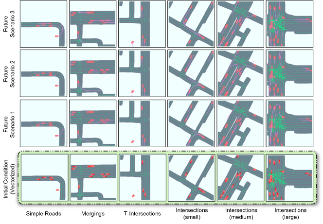
Figure 5: Qualitative evaluation of the different possible future scenarios generated from the same initial scene. Comparing the scenarios in each column, each future scenario presents distinct agent behaviors starting from the same initial scene.

Ablation Study. The fidelity and diversity scores of various ablated versions of our method are presented in TABLE I. While maintaining a constant input resolution, rectangular areas of different sizes are extracted from ground truth scenarios to train and evaluate each ablated version. The fidelity and diversity results indicate that DriveSceneGen is not sensitive to the changes in the range of the scenario.

IV-C Vectorization Fidelity

Baselines. To evaluate the performance of our vectorization pipeline, two other baseline methods were proposed and compared: (1) a Transformer-based model and (2) a graph-based method without intersection curve fitting.

For the Transformer-based method, a variant of the DETR[25] detector is designed for extracting lane vectors from the BEV feature maps. In line with the method described in LaneGAP[26], the initial raw ground truth polylines are assembled as a path that traverses the map from one edge to another. A hierarchical query is also implemented for the transformer decoder, explicitly encoding centerline elements for enhanced accuracy[27].

Quantitative Evaluation. Two graph-based metrics are selected to assess the fidelity of vectorization, namely GEO and TOPO metric [28]. The GEO-metric compares the geometric accuracy and recall between the vectorized results and the ground truth, while the TOPO-metric further considers the topological connectivity as well. The vectorization process is evaluated on the Waymo dataset since the generated initial scenes do not have their corresponding ground truth data. For each ground truth feature map $F$, we predict the vectorized data $\mathcal{M}_{pred}$ and compare it with the ground truth data $\mathcal{M}$.

During the evaluation, each path is interpolated to intervals of 0.5$m$. For the ground truth graph $G$, and extraction result $\hat{G}$, two vertices are paired if their distance is smaller than 1.5$m$. The subgraph distance $r$ is 50$m$. Experiments are conducted on 1$k$ ground truth examples, and results are listed in TABLE II. Results indicate that the Graph-fitting method has the highest vectorization fidelity. The graph-based approach outperforms the DETR-path method as it directly extracts polylines from the pixels. Furthermore, the graph-based method exhibits less degradation in performance as the scenario size increases. The Graph-fitting method excels in accurately fitting lane shapes, resulting in a significant improvement in the Precision scores. By comparing the results of different map ranges, a recommended range of 80$m$ is concluded to strike a balance between scenario size and vectorization accuracy.

TABLE II: Fidelity of Vectorized Samples

Method	GEO Metric			TOPO Metric
	Pre	Rec	F1	Pre	Rec	F1
DETR-path 40m	0.64	0.81	0.72	0.56	0.57	0.56
DETR-path 80m	0.52	0.67	0.59	0.37	0.33	0.35
DETR-path 120m	0.41	0.53	0.46	0.22	0.18	0.20
Graph 40m	0.70	0.86	0.77	0.59	0.75	0.66
Graph 80m	0.65	0.78	0.71	0.50	0.63	0.56
Graph 120m	0.64	0.56	0.60	0.47	0.37	0.42
Graph-fitting 40m	0.95	0.86	0.91	0.92	0.67	0.77
Graph-fitting 80m	0.92	0.85	0.88	0.88	0.56	0.68
Graph-fitting 120m	0.90	0.82	0.86	0.86	0.47	0.60

IV-D Simulation Results

Qualitative Evaluation. For this experiment, the simulation model is trained on the same Waymo Motion dataset. Based on the experiment results in the previous section, the scenario range is set as 80$m$. For each generated and vectorized initial scene $\{\mathcal{\hat{M}},\mathcal{\hat{A}}\}$, the top 3 future trajectories are generated by the simulation model and visualized in Fig. 5. By comparing the scenarios in each column, it can be observed that each future scenario presents distinct agent behaviors starting from the same initial scene.

V CONCLUSIONS & DISCUSSION

In this paper, we present the first method that learns to generate driving scenarios from the collected real-world driving dataset from scratch. Our method demonstrates that the task of generating novel driving scenarios that comply with real-world distributions is possible. Experimental results highlight the capability of DriveSceneGen in generating quality, diversity, and scalability on real-world datasets. We believe that such capability can potentially benefit the development of data-driven methods in autonomous driving and have unlimited prospective applications outside robotics. Since the generation of an entire dynamic scenario is a new task, there are currently no quantitative metrics to directly compare the distribution of the generated dynamic scenarios consisting of both maps and agent behaviors to the ground truth distribution. We wish to investigate potential metrics as part of our future work.

References

- [1] S. Ettinger, S. Cheng, B. Caine, C. Liu, H. Zhao, S. Pradhan, Y. Chai, B. Sapp, C. Qi, Y. Zhou, Z. Yang, A. Chouard, P. Sun, J. Ngiam, V. Vasudevan, A. McCauley, J. Shlens, and D. Anguelov, “Large Scale Interactive Motion Forecasting for Autonomous Driving : The Waymo Open Motion Dataset,” Proceedings of the IEEE International Conference on Computer Vision, pp. 9690–9699, apr 2021. [Online]. Available: https://arxiv.org/abs/2104.10133v1
- [2] H. Caesar, J. Kabzan, K. S. Tan, W. K. Fong, E. M. Wolff, A. H. Lang, L. Fletcher, O. Beijbom, and S. Omari, “nuplan: A closed-loop ml-based planning benchmark for autonomous vehicles,” CoRR, vol. abs/2106.11810, 2021. [Online]. Available: https://arxiv.org/abs/2106.11810
- [3] M.-F. Chang, J. Lambert, P. Sangkloy, J. Singh, S. Bak, A. Hartnett, D. Wang, P. Carr, S. Lucey, D. Ramanan, and J. Hays, “Argoverse: 3d tracking and forecasting with rich maps,” in Proceedings of the IEEE/CVF Conference on Computer Vision and Pattern Recognition (CVPR), June 2019.
- [4] B. Wilson, W. Qi, T. Agarwal, J. Lambert, J. Singh, S. Khandelwal, B. Pan, R. Kumar, A. Hartnett, J. Kaesemodel Pontes, D. Ramanan, P. Carr, and J. Hays, “Argoverse 2: Next generation datasets for self-driving perception and forecasting,” in Proceedings of the Neural Information Processing Systems Track on Datasets and Benchmarks, J. Vanschoren and S. Yeung, Eds., vol. 1. Curran, 2021. [Online]. Available: https://datasets-benchmarks-proceedings.neurips.cc/paper_files/paper/2021/file/4734ba6f3de83d861c3176a6273cac6d-Paper-round2.pdf
- [5] U. S. D. o. T. Federal Highway Administration, “Average annual miles per driver by age group.” [Online]. Available: https://www.fhwa.dot.gov/ohim/onh00/bar8.htm
- [6] J. Sohl-Dickstein, E. A. Weiss, N. Maheswaranathan, and S. Ganguli, “Deep unsupervised learning using nonequilibrium thermodynamics,” 2015.
- [7] J. Ho, A. Jain, and P. Abbeel, “Denoising diffusion probabilistic models,” 2020.
- [8] R. Rombach, A. Blattmann, D. Lorenz, P. Esser, and B. Ommer, “High-resolution image synthesis with latent diffusion models,” 2022.
- [9] A. Lugmayr, M. Danelljan, A. Romero, F. Yu, R. Timofte, and L. V. Gool, “Repaint: Inpainting using denoising diffusion probabilistic models,” 2022.
- [10] S. Gong, M. Li, J. Feng, Z. Wu, and L. Kong, “DiffuSeq: Sequence to Sequence Text Generation with Diffusion Models,” oct 2022. [Online]. Available: http://arxiv.org/abs/2210.08933
- [11] Z. Kong, W. Ping, J. Huang, K. Zhao, and B. Catanzaro, “Diffwave: a Versatile Diffusion Model for Audio Synthesis,” ICLR 2021 - 9th International Conference on Learning Representations, 2021.
- [12] A. Ajay, Y. Du, A. Gupta, J. Tenenbaum, T. Jaakkola, and P. Agrawal, “Is Conditional Generative Modeling all you need for Decision-Making?” nov 2022. [Online]. Available: http://arxiv.org/abs/2211.15657
- [13] M. Janner, Y. Du, J. B. Tenenbaum, and S. Levine, “Planning with Diffusion for Flexible Behavior Synthesis,” Proceedings of Machine Learning Research, vol. 162, pp. 9902–9915, 2022.
- [14] G. Tevet, S. Raab, B. Gordon, Y. Shafir, D. Cohen-Or, and A. H. Bermano, “Human motion diffusion model,” 2022.
- [15] S. Azizi, S. Kornblith, C. Saharia, M. Norouzi, and D. J. Fleet, “Synthetic Data from Diffusion Models Improves ImageNet Classification,” apr 2023. [Online]. Available: https://arxiv.org/abs/2304.08466v1
- [16] S. Tan, K. Wong, S. Wang, S. Manivasagam, M. Ren, and R. Urtasun, “SceneGen: Learning to Generate Realistic Traffic Scenes,” Proceedings of the IEEE Computer Society Conference on Computer Vision and Pattern Recognition, pp. 892–901, 2021.
- [17] L. Bergamini, Y. Ye, O. Scheel, L. Chen, C. Hu, L. Del Pero, B. Osiński, H. Grimmett, and P. Ondruska, “Simnet: Learning Reactive Self-driving Simulations from Real-world Observations,” Proceedings - IEEE International Conference on Robotics and Automation, vol. 2021-May, pp. 5119–5125, 2021.
- [18] L. Feng, Q. Li, Z. Peng, S. Tan, and B. Zhou, “TrafficGen: Learning to Generate Diverse and Realistic Traffic Scenarios,” 2022. [Online]. Available: http://arxiv.org/abs/2210.06609
- [19] L. Mi, H. Zhao, C. Nash, X. Jin, J. Gao, C. Sun, C. Schmid, N. Shavit, Y. Chai, and D. Anguelov, “Hdmapgen: A hierarchical graph generative model of high definition maps,” in Proceedings of the IEEE/CVF Conference on Computer Vision and Pattern Recognition, 2021, pp. 4227–4236.
- [20] O. Ronneberger, P. Fischer, and T. Brox, “U-net: Convolutional networks for biomedical image segmentation,” 2015.
- [21] T. Y. Zhang and C. Y. Suen, “A fast parallel algorithm for thinning digital patterns,” Commun. ACM, vol. 27, no. 3, p. 236–239, mar 1984. [Online]. Available: https://doi.org/10.1145/357994.358023
- [22] S. Shi, L. Jiang, D. Dai, and B. Schiele, “Motion transformer with global intention localization and local movement refinement,” 2023.
- [23] M. Heusel, H. Ramsauer, T. Unterthiner, B. Nessler, and S. Hochreiter, “Gans trained by a two time-scale update rule converge to a local nash equilibrium,” Advances in neural information processing systems, vol. 30, 2017.
- [24] H.-Y. Lee, X. Yang, M.-Y. Liu, T.-C. Wang, Y.-D. Lu, M.-H. Yang, and J. Kautz, “Dancing to music,” 2019.
- [25] N. Carion, F. Massa, G. Synnaeve, N. Usunier, A. Kirillov, and S. Zagoruyko, “End-to-end object detection with transformers,” in European conference on computer vision. Springer, 2020, pp. 213–229.
- [26] B. Liao, S. Chen, B. Jiang, T. Cheng, Q. Zhang, W. Liu, C. Huang, and X. Wang, “Lane graph as path: Continuity-preserving path-wise modeling for online lane graph construction,” arXiv preprint arXiv:2303.08815, 2023.
- [27] B. Liao, S. Chen, X. Wang, T. Cheng, Q. Zhang, W. Liu, and C. Huang, “Maptr: Structured modeling and learning for online vectorized hd map construction,” in International Conference on Learning Representations, 2023.
- [28] S. He and H. Balakrishnan, “Lane-level street map extraction from aerial imagery,” in Proceedings of the IEEE/CVF Winter Conference on Applications of Computer Vision, 2022, pp. 2080–2089.