FedCompass: Efficient Cross-Silo Federated Learning on Heterogeneous Client Devices using a Computing Power Aware Scheduler

Abstract

Cross-silo federated learning offers a promising solution to collaboratively train robust and generalized AI models without compromising the privacy of local datasets, e.g., healthcare, financial, as well as scientific projects that lack a centralized data facility. Nonetheless, because of the disparity of computing resources among different clients (i.e., device heterogeneity), synchronous federated learning algorithms suffer from degraded efficiency when waiting for straggler clients. Similarly, asynchronous federated learning algorithms experience degradation in the convergence rate and final model accuracy on non-identically and independently distributed (non-IID) heterogeneous datasets due to stale local models and client drift. To address these limitations in cross-silo federated learning with heterogeneous clients and data, we propose FedCompass, an innovative semi-asynchronous federated learning algorithm with a computing power aware scheduler on the server side, which adaptively assigns varying amounts of training tasks to different clients using the knowledge of the computing power of individual clients. FedCompass ensures that multiple locally trained models from clients are received almost simultaneously as a group for aggregation, effectively reducing the staleness of local models. At the same time, the overall training process remains asynchronous, eliminating prolonged waiting periods from straggler clients. Using diverse non-IID heterogeneous distributed datasets, we demonstrate that FedCompass achieves faster convergence and higher accuracy than other asynchronous algorithms while remaining more efficient than synchronous algorithms when performing federated learning on heterogeneous clients.

1 Introduction

Federated learning (FL) is a collaborative model training approach where multiple clients train a global model under the orchestration of a central server (Konečnỳ et al., 2016; McMahan et al., 2017; Yang et al., 2019; Kairouz et al., 2021). In FL, there are $m$ distributed clients solving the optimization problem: $\min_{w\in\mathbb{R}^{d}}F(w)=\sum_{i=1}^{m}p_{i}F_{i}(w),$ where $p_{i}$ is the importance weight of client $i$’s local data and is usually defined as the relative data sample size, and $F_{i}(w)$ is the loss on client $i$’s local data. FL typically runs two steps iteratively: (i) the server distributes the global model to clients to train it using their local data; (ii) the server collects the locally trained models and updates the global model by aggregating them. Federated Averaging (FedAvg) (McMahan et al., 2017) is the most popular FL algorithm where each client trains a model using local data for $Q$ local steps in each training round, after which the orchestration server aggregates all local models by performing a weighted averaging and sends the updated global model back to all clients for the next round of training. By leveraging the training data from multiple clients without explicitly sharing, FL empowers the training of more robust and generalized models while preserving the privacy of client data. The data in FL is generally heterogeneous, which means that client data is non-identically and independently distributed (non-IID). FL is most commonly conducted in two settings: cross-device FL and cross-silo FL (Kairouz et al., 2021). In cross-device FL, numerous mobile or IoT devices participate, but not in every training round due to reliability issues (Mills et al., 2019). In cross-silo FL, a smaller number of reliable clients contribute to training in each round, and the clients are often represented by large institutions in domains such as healthcare or finance, where it is essential to preserve data privacy (Wang et al., 2019; Wang, 2019; Kaissis et al., 2021; Pati et al., 2022).

The performance of FL suffers from device heterogeneity, where the disparity of computing power among participating client devices leads to significant variations in local training times. Classical synchronous FL algorithms such as FedAvg, where the server waits for all client models before global aggregation, suffer from compute inefficiency as faster clients have to wait for slower clients (stragglers). Several asynchronous FL algorithms have been developed to immediately update the global model after receiving one client model to improve computing resource utilization. The principal shortcoming in asynchronous FL is straggler clients may train on outdated global models and obtain stale local models, which can potentially undermine the performance of the global model. To deal with stale local models, various solutions have been proposed, including client selection, weighted aggregation, and tiered FL. Client selection strategies such as FedAR (Imteaj & Amini, 2020) select a subset of clients according to their robustness or computing power. However, these strategies may not be applicable for cross-silo FL settings, where all clients are expected to participate to maintain the robustness of the global model. Algorithms such as FedAsync (Xie et al., 2019) introduce a staleness factor to penalize the local models trained on outdated global models. While the staleness factor alleviates the negative impact of stale local models, it may cause the global model to drift away from the slower clients (client drift) even with minor disparities in client computing power, resulting in a further decrease in accuracy on non-IID heterogeneous distributed datasets. Tiered FL methods such as FedAT (Chai et al., 2021) group clients into tiers based on their computing power, allowing each tier to update at its own pace. Nonetheless, the waiting time inside each tier can be significant, and it is not resilient to sudden changes in computing power.

In this paper, we focus on improving the performance in cross-silo FL settings. Particularly, we propose a semi-asynchronous cross-silo FL algorithm, FedCompass, which employs a COMputing Power Aware Scheduler (Compass) to reduce client local model staleness and enhance FL efficiency in cross-silo settings. Compass assesses the computing power of individual clients based on their previous response times and dynamically assigns varying numbers of local training steps to ensure that a group of clients can complete local training almost simultaneously. Compass is also designed to be resilient to sudden client computing power changes. This enables the server to perform global aggregation using the local models from a group of clients without prolonged waiting times to improve computing resource utilization. Group aggregation leads to less global update frequency and reduced local model staleness, thus mitigating client drift and improving the performance on non-IID heterogeneous data. In addition, the design of FedCompass is orthogonal to and compatible with several server-side optimization strategies for further enhancement of performance on non-IID data. In summary, the main contributions of this paper are:

• A novel semi-asynchronous cross-silo FL algorithm, FedCompass, which employs a resilient computing power aware scheduler to make client updates arrive in groups almost simultaneously for aggregation, thus reducing client model staleness for enhanced performance on non-IID heterogeneous distributed datasets while ensuring computing efficiency.

• A suite of convergence analyses which demonstrate that FedCompass can converge to a first-order critical point of the global loss function with heterogeneous clients and data, and offer insights into how the number of local training steps impacts the convergence rate.

• A suite of experiments with heterogeneous clients and datasets which demonstrate that FedCompass converges faster than synchronous and asynchronous FL algorithms, and achieves higher accuracy than other asynchronous algorithms by mitigating client drift.

2 Related Work

Device Heterogeneity in Federated Learning. Device heterogeneity occurs when clients have varying computing power, leading to varied local training times (Li et al., 2020; Xu et al., 2021). For synchronous FL algorithms that wait for all local models before global aggregation, device heterogeneity leads to degraded efficiency due to the waiting time for slower clients, often referred to as stragglers. Some methods address device heterogeneity by only waiting for some clients and ignoring the stragglers (Bonawitz et al., 2019). However, this approach disregards the contributions of straggler clients, resulting in wasted client computing resources and a global model significantly biased towards faster clients. Other solutions explicitly select the clients that perform updates. Chen et al. (2021) employs a greedy selection method as a heuristic based on client computing resources. Hao et al. (2020) defines a priority function according to computing power and model accuracy to select participating clients. FedAr (Imteaj & Amini, 2020) assigns each client a trust score based on previous activities. FedCS (Nishio & Yonetani, 2019) queries client resource information for client selection. SAFA (Wu et al., 2020) chooses the clients with lower crash probabilities. However, these methods may not be suitable for cross-silo FL settings, where the participation of every client is crucial for maintaining the robustness of the global model and there are stronger assumptions with regard to the trustworthiness and reliability of clients.

Asynchronous Federated Learning. Asynchronous FL algorithms provide another avenue to mitigate the impact of stragglers. In asynchronous FL, the server typically updates the global model once receiving one or few client models (Xie et al., 2019; Chen et al., 2020) or stores the local models in a size-$K$ buffer (Nguyen et al., 2022), and then immediately sends the global model back for further local training. Asynchronous FL offers significant advantages in heterogeneous client settings by reducing the idle time for each client. However, one of the key challenges in asynchronous FL is the staleness of local models. In asynchronous FL, global model updates can occur without waiting for all local models. This flexibility leads to stale local models trained on outdated global models, which may negatively impact the accuracy of the global model. Various solutions aimed to mitigate these adverse effects are proposed. One common strategy is weighted aggregation, which is prevalent in numerous asynchronous FL algorithms (Xie et al., 2019; Chen et al., 2019; 2020; Wang et al., 2021; Nguyen et al., 2022). This approach applies a staleness weight factor to penalize outdated local models during the aggregation. While effective in reducing the negative impact of stale models, this often causes the global model to drift away from the local data on slower clients, and the staleness factor could significantly degrade the final model performance in settings with minor computing disparities among clients. Tiered FL methods offer another option for improvement. FedAT (Chai et al., 2021) clusters clients into several faster and slower tiers, allowing each tier to update the global model at its own pace. However, the waiting time within tiers can be substantial, and it becomes less effective when the client pool is small. The tiering may also not get updated timely to become resilient to speed changes. Similarly, CSAFL (Zhang et al., 2021) groups clients based on gradient direction and computation time. While this offers some benefits, the fixed grouping can become a liability if client computing speeds vary significantly over the course of training.

3 Proposed Method: FedCompass

The design choices of FedCompass are motivated by the shortcomings of other asynchronous FL algorithms and the desire to specifically adapt FedCompass for the cross-silo FL settings. The potential staleness of client local models is the main challenge for asynchronous FL algorithms. In FedAsync, as the global model gets updated frequently, the client model is significantly penalized by a staleness weight factor, leading to theoretically and empirically sub-optimal convergence characteristics, especially when the disparity in computing power amongst clients is small. This can cause the global model to gradually drift away from the data of slow clients and have decreased performance on non-IID heterogeneous distributed datasets. FedBuffer attempts to address this problem by introducing a size-$K$ buffer for client updates to reduce the global update frequency. However, the optimal buffer size varies for different client numbers and heterogeneity settings and needs to be selected heuristically. It is also possible that one buffer contains several updates from the same client, or one client may train on the same global model several times. Inspired by those shortcomings, we aim to group clients for global aggregation to reduce model staleness and avoid repeated aggregation or local training. As cross-silo FL involves a small number of reliable clients, this enables us to design a scheduler that can profile the computing power of each client. The scheduler then dynamically and automatically creates groups accordingly by assigning clients with different numbers of local training steps to allow clients with similar computing power to finish local training in close proximity to each other. Additionally, we decide to keep the scheduler operations separated from the global aggregation, which makes it possible to combine the benefits of aggregation strategies in other FL algorithms, such as server-side optimizations for improving performance when training data are non-IID (Hsu et al., 2019; Reddi et al., 2020). Finally, learning from the drawbacks of other tiered FL methods such as FedAT and CSAFL, we also design the scheduler to cover multiple corner cases to ensure its resilience to sudden changes in client computing power.

3.1 Compass: Computing Power Aware Scheduler

To address the aforementioned desiderata, we introduce a COMputing Power Aware Scheduler (Compass), which assesses the computing power of individual clients according to their previous response times. Compass then dynamically assigns varying numbers of local steps $Q$ within a predefined range $[Q_{\min},Q_{\max}]$ to different clients in each training round. This approach ensures that multiple client models are received nearly simultaneously, allowing for a grouped aggregation on the server side. By incorporating several local models in a single global update and coordinating the timing of client responses, we effectively reduce the frequency of global model updates. This, in turn, reduces client model staleness while keeping the client idle time to a minimum during the training process.

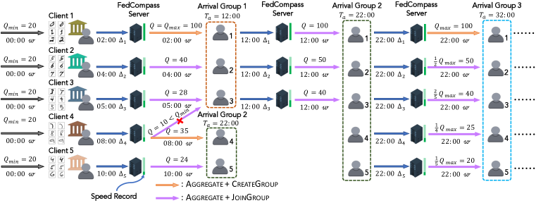
Figure 1: Overview of an example FL run using Compass scheduler on five clients with the minimum number of local steps $Q_{\min}=20$ and maximum number of local steps $Q_{\max}=100$.

Figure 1 illustrates an example run of federated learning using Compass scheduler on five clients with different computing power. For the sake of brevity, this illustration focuses on a simple scenario, and more details are described in Section 3.2. All times in the figure are absolute wall-clock times from the start of FL. First, all clients are initialized with $Q_{\min}=20$ local steps. When client 1 finishes local training and sends the update $\Delta_{1}$ to the server at time 02:00, Compass records its speed and creates the first arrival group with the expected arrival time ${T}_{a}=$ 12:00, which is computed based on the client speed and the assigned number of local steps $Q=Q_{\max}=100$. We assume negligible communication and aggregation times in this example, so client 1 receives an updated global model $w$ immediately at 02:00 and begins the next round of training. Upon receiving the update from client 2, Compass slots it into the first arrival group with $Q=40$ local steps, aiming for a completion time of $T_{a}=$ 12:00 as well. Client 3 follows suit with $28$ steps. When Compass computes local steps for client 4 in order to finish by ${T}_{a}=$ 12:00, it finds that $Q=10$ falls below $Q_{\min}=20$. Therefore, Compass creates a new arrival group for client 4 with expected arrival time $T_{a}=$ 22:00. Compass optimizes the value of $T_{a}$ such that the clients in an existing arrival group may join this newly created group in the future for group merging. After client 5 finishes, it is assigned to the group created for client 4. When clients 1-3 finish their second round of local training at 12:00, Compass assigns them to the arrival group of clients 4 and 5 (i.e., arrival group 2) with the corresponding values of $Q$ so that all the clients are in the same arrival group and expected to arrive nearly simultaneously for global aggregation in the future. The training then achieves equilibrium, and future training rounds will proceed with certain values of $Q$ for each client in the ideal case.

The detailed implementation and explanation of Compass can be found in Appendix A. We also provide analyses and empirical results for non-ideal scenarios with client computing powering changes in Appendix G.2, where we show how the design of Compass makes it resilient when clients experience speedup or slowdown during the course of training.

3.2 FedCompass: Federated Learning with Compass

1

2Function FedCompass-Client($i$, $w$, $Q$, $\eta_{\ell}$, $B$):

Input : Client id $i$, global model $w$, number of local steps $Q$, local learning rate $\eta_{\ell}$, batch size $B$

3 for $q\in[1,\dots,Q]$ do

4       $\mathcal{B}_{i,q}:=$ random training batch with batch size $B$;

5       $w_{i,q}:=w_{i,q-1}-\eta_{\ell}\nabla f_{i}(w_{i,q-1},\mathcal{B}_{i,q})$ $\ \triangleright$ $w_{i,q}$ is client $i$’s model after $q$ steps, $w_{i,0}=w$;

6      

7Send $\Delta_{i}:=w_{i,0}-w_{i,Q}$ to server;

8

9

10Function FedCompass-Server($N$, $\eta_{\ell}$, $B$, $w$):

Input : Number of comm. rounds $N$, local learning rate $\eta_{\ell}$, batch size $B$, initial model weight $w$

11 $\textsc{FedCompass-Client}(i,w,Q_{\min},\eta_{\ell},B)$ for all client $i$’s;

12 Initialize client info dictionary $\mathcal{C}$, group info dictionary $\mathcal{G}$, and global model timestamp $\tau_{g}:=0$;

13 for $n\in[1,\dots,N]$ do

14       if receive update $\Delta_{i}$ from client $i$ then

15             Record client speed into $\mathcal{C}\texttt{[}i\texttt{]}.S$;

16             if client $i$ has an arrival group $g$ then

17                  

18                  $\mathcal{G}\texttt{[}g\texttt{]}.CL.\texttt{remove(}i\texttt{)}$,  $\mathcal{G}\texttt{[}g\texttt{]}.ACL.\texttt{add(}i\texttt{)}$ $\ \triangleright$ move client $i$ to arrived client list;

19                   if $T_{\text{now}}>\mathcal{G}\texttt{[}g\texttt{]}.{T}_{\max}$ then

20                         $\overline{\Delta}:=\overline{\Delta}+st(\tau_{g}-\mathcal{C}\texttt{[}i\texttt{]}.\tau)*p_{i}*\Delta_{i}$;  $\mathcal{C}\texttt{[}i\texttt{]}.\tau:=\tau_{g}$;

21                         $\textsc{AssignGroup}(i)$ $\ \triangleright$ this computes $\mathcal{C}\texttt{[}i\texttt{]}.Q$, details in Alg. 2 from Appendix;

22                         FedCompass-Client $(i,w,\mathcal{C}\texttt{[}i\texttt{]}.Q,\eta_{\ell},B)$;

23                         delete $\mathcal{G}\texttt{[}g\texttt{]}$ if $\texttt{len(}\mathcal{G}\texttt{[}g\texttt{]}.CL\texttt{)}=0$;

24                        

25                  else

26                         $\overline{\Delta}^{g}:=\overline{\Delta}^{g}+st(\tau_{g}-\mathcal{C}\texttt{[}i\texttt{]}.\tau)*p_{i}*\Delta_{i}$;

27                         if $\texttt{len(}\mathcal{G}\texttt{[}g\texttt{]}.CL=0\texttt{)}$ then

28                               $\textsc{GroupAggregate}(g)$ $\ \triangleright$ details in Alg. 3 from Appendix;

29                               delete $\mathcal{G}\texttt{[}g\texttt{]}$;

30                              

31                        

32                  

33            else

34                   $w:=w-st(\tau_{g}-\mathcal{C}\texttt{[}i\texttt{]}.\tau)*p_{i}*\Delta_{i}$;  $\tau_{g}:=\tau_{g}+1$;  $\mathcal{C}\texttt{[}i\texttt{]}.\tau:=\tau_{g}$;

35                   $\textsc{AssignGroup}(i)$ $\ \triangleright$ this computes $\mathcal{C}\texttt{[}i\texttt{]}.Q$, details in Alg. 2 from Appendix;

36                   FedCompass-Client $(i,w,\mathcal{C}\texttt{[}i\texttt{]}.Q,\eta_{\ell},B)$;

37                  

38            

39      

Algorithm 1 FedCompass Algorithm

FedCompass is a semi-asynchronous FL algorithm that leverages the Compass scheduler to coordinate the training process. It is semi-asynchronous as the server may need to wait for a group of clients for global aggregation, but the Compass scheduler minimizes the waiting time by managing to have clients within the same group to finish local training nearly simultaneously, so the overall training process still remains asynchronous without long client idle times. Function FedCompass-Client in Algorithm 1 outlines the client-side algorithm for FedCompass. The client performs $Q$ local steps using mini-batch stochastic gradient descent and sends the difference between the initial and final models $\Delta_{i}$ as the client update to the server.

Function FedCompass-Server in Algorithm 1 presents the algorithm for FedCompass server. The server records the client and arrival group information in dictionaries $\mathcal{C}$ and $\mathcal{G}$. As the server has no prior knowledge of the computing power of clients, it first assigns $Q_{\min}$ local steps to all clients for warm-up. The client’s computing speed is updated according to the training time and the number of local steps whenever the server receives an update from the client (line 12). If client $i$ belongs to an arrival group $g$, the server will move the client from the list of non-arrived clients ($\mathcal{G}\texttt{[}g\texttt{]}.CL$) to the list of arrived clients ($\mathcal{G}\texttt{[}g\texttt{]}.ACL$). In addition to the expected arrival time $\mathcal{G}\texttt{[}g\texttt{]}.T_{a}$, each group $g$ has the latest arrival time $\mathcal{G}\texttt{[}g\texttt{]}.T_{\max}$ to account for client speed fluctuations and estimation errors. If the client arrives later than $\mathcal{G}\texttt{[}g\texttt{]}.{T}_{\max}$ (lines 15 to 19), the server stores the update in a general buffer $\overline{\Delta}$ with a staleness factor $st(\cdot)$ applied, which is computed based on the difference between the global model timestamp ($\tau_{g}$) and the local model timestamp ($\mathcal{C}\texttt{[}i\texttt{]}.\tau$). The server then immediately assigns a new training task to the client after assigning an arrival group (see Alg. 2 in Appendix A for details of AssignGroup). When the client arrives earlier than $\mathcal{G}\texttt{[}g\texttt{]}.{T}_{\max}$ (lines 20 to 24), the server stores the client update into a group-specific buffer $\overline{\Delta}^{g}$ with the staleness factor applied, and checks whether the client is the last one in the group to arrive. If not, the server waits until the last client in the group arrives or the latest arrival time $\mathcal{G}\texttt{[}g\texttt{]}.{T}_{\max}$. Otherwise, the server invokes GroupAggregate for global aggregation. GroupAggregate updates the global model using the group-specific butter $\overline{\Delta}^{g}$ and the general buffer $\overline{\Delta}$, and assigns new training tasks to all arriving clients in the group $g$. The details of GroupAggregate are shown in Algorithm 3 in the Appendix. If client $i$ does not belong to any arrival group (lines 25 to 28), which only occurs when client $i$ arrives for the first time after the warm-up, the server immediately updates the global model, assigns an arrival group, and sends a new training task to client $i$.

4 Convergence Analysis

We provide the convergence analysis of FedCompass for smooth and non-convex loss functions $F_{i}(w)$. We denote by $\nabla F(w)$ the gradient of global loss, $\nabla F_{i}(w)$ the gradient of client $i$’s local loss, and $\nabla f_{i}(w,\mathcal{B}_{i})$ the gradient of loss evaluated on batch $\mathcal{B}_{i}$. With that, we make the following assumptions.

Assumption 1.

Lipschitz smoothness. The loss function of each client $i$ is Lipschitz smooth. $||\nabla F_{i}(w)-\nabla F_{i}(w^{\prime})||\leq L||w-w^{\prime}||$.

Assumption 2.

Unbiased client stochastic gradient. $\mathbb{E}_{\mathcal{B}_{i}}[\nabla f_{i}(w,\mathcal{B}_{i}))]=\nabla F_{i}(w)$.

Assumption 3.

Bounded gradient, and bounded local and global gradient variance. $||\nabla F_{i}(w)||^{2}\leq M$, $\mathbb{E}_{\mathcal{B}_{i}}[||\nabla f_{i}(w,\mathcal{B}_{i}))-\nabla F_{i}(w)||^{2}]\leq\sigma_{l}^{2}$, and $\mathbb{E}[||\nabla F_{i}(w)-\nabla F(w)||^{2}]\leq\sigma_{g}^{2}$.

Assumption 4.

Bounded client heterogeneity and staleness. Suppose that client $a$ is the fastest client, and client $b$ is the slowest, $\mathcal{T}_{a}$ and $\mathcal{T}_{b}$ are the times per one local step of these two clients, respectively. We then assume that ${\mathcal{T}_{b}}/{\mathcal{T}_{a}}\leq\mu$. This assumption also implies that the staleness ($\tau_{g}-\mathcal{C}\texttt{[}i\texttt{]}.\tau$) of each client model is also bounded by a number $\tau_{\max}$.

Assumptions 1-3 are common assumptions in the convergence analysis of federated or distributed learning algorithms (Stich, 2018; Li et al., 2019; Yu et al., 2019; Karimireddy et al., 2020; Nguyen et al., 2022). Assumption 4 indicates that the speed difference among clients is finite and is equivalent to the assumption that all clients are reliable, which is reasonable in cross-silo FL.

Theorem 1.

Suppose that $\eta_{\ell}\leq\frac{1}{2LQ_{\max}}$, $\textit{Q}=Q_{\max}/Q_{\min}$, and $\mu^{\prime}=\textit{Q}^{\lfloor\log_{\textit{Q}}\mu\rfloor}$. Then, after $T$ updates for global model $w$, FedCompass achieves the following convergence rate:

$$\frac{1}{T}\mathop{\sum}\limits_{t=0}^{T-1}\mathbb{E}\|\nabla F(w^{(t)})\|^{2}\leq \frac{2\gamma_{2}F^{*}}{\eta_{\ell}Q_{\min}T}+\frac{2\gamma_{2}\eta_{\ell}m^{2}\sigma_{l}^{2}LQ_{\max}^{2}}{\gamma_{1}^{2}Q_{\min}}+\frac{6\gamma_{2}m\eta_{\ell}^{2}\sigma^{2}L^{2}Q_{\max}^{3}}{\gamma_{1}Q_{\min}}(\tau_{\max}^{2}+1),$$ (1)

where $m$ being the number of clients, $w^{(t)}$ being the global model after $t$ global updates, $\gamma_{1}=1+\frac{m-1}{\mu^{\prime}},\gamma_{2}=1+\mu^{\prime}(m-1)$, $F^{*}=F(w^{(0)})-F(w^{*})$, and $\sigma^{2}=\sigma_{l}^{2}+\sigma_{g}^{2}+M$.

Corollary 1.

When $Q_{\min}\leq{Q_{\max}}/{\mu}$ and $\eta_{\ell}=\mathcal{O}(1/Q_{\max}\sqrt{T})$ while satisfying $\eta_{\ell}\leq\frac{1}{2LQ_{\max}}$, then

$$\underset{t\in[T]}{\min}\ \mathbb{E}\|\nabla F(w^{(t)})\|^{2}\leq\mathcal{O}\Big{(}\frac{mF^{*}}{\sqrt{T}}\Big{)}+\mathcal{O}\Big{(}\frac{m\sigma_{l}^{2}L}{\sqrt{T}}\Big{)}+\mathcal{O}\Big{(}\frac{m\tau_{\max}^{2}\sigma^{2}L^{2}}{T}\Big{)}$$ (2)

The proof is provided in Appendix C. Based on Theorem 1 and Corollary 1, we remark the following algorithmic characteristics.

Worst Case Convergence. Corollary 1 provides an upper bound for the expected squared norm of the gradients of the global loss, which is monotonically decreasing with respect to the total number of global updates $T$. This leads to the conclusion that FedCompass converges to a first-order stationary point in expectation, characterized by a zero gradient, of the smooth and non-convex global loss function $F(w)=\sum_{i=1}^{m}p_{i}F_{i}(w)$. Specifically, the first term of (2) represents the influence of model initialization, and the second term accounts for stochastic noise from local updates. The third term reflects the impact of device heterogeneity ($\tau_{\max}^{2}$) and data heterogeneity ($\sigma^{2}$) on the convergence process, which theoretically provides a convergence guarantee for FedCompass on non-IID heterogeneous distributed datasets and heterogeneous client devices.

Effect of Number of Local Steps. Theorem 1 establishes the requirement $\eta_{\ell}\leq\frac{1}{2LQ_{\max}}$, signifying a trade-off between the maximum number of client local steps $Q_{\max}$ and the client learning rate $\eta_{\ell}$. A higher $Q_{\max}$ necessitates a smaller $\eta_{\ell}$ to ensure the convergence of FL training. The value of $Q_{\min}$ also presents a trade-off: a smaller $Q_{\min}$ leads to a reduced $\mu^{\prime}$, causing an increase in $\gamma_{1}$ and a decrease in $\gamma_{2}$, which ultimately lowers the gradient bound. Appendix B shows that $Q_{\min}$ also influences the grouping of FedCompass. There are at most $\lceil\log_{\textit{Q}}\mu\rceil$ existing groups at the equilibrium state, so a smaller $Q_{\min}$ results in fewer groups and a smaller $\tau_{\max}$. However, as $Q_{\min}$ appears in the denominator in (1), a smaller $Q_{\min}$ could potentially increase the gradient bound. Corollary 1 represents an extreme case where the value of $Q_{\min}$ makes $\mu^{\prime}$ reach the minimum value of 1. We give empirical ablation study results on the effect of the number of local steps in Section 5.2 and Appendix G.1. The ablation study results show that the performance of FedCompass is not sensitive to the choice of the ratio $\textit{Q}=Q_{\max}/Q_{\min}$, and a wide range of Q still leads to better performance than other asynchronous FL algorithms such as FedBuffer.

5 Experiments

5.1 Experiment Setup

Datasets. To account for the inherent statistical heterogeneity of federated datasets, we use two types of datasets: (i) artificially partitioned MNIST (LeCun, 1998) and CIFAR-10 (Krizhevsky et al., 2009) datasets, and (ii) two naturally split datasets from cross-silo FL benchmark FLamby (Ogier du Terrail et al., 2022), Fed-IXI and Fed-ISIC2019. Artificially partitioned datasets are created by dividing classic datasets into client splits. We introduce class partition and dual Dirichlet partition strategies. The class partition makes each client only hold data of a few classes, and the dual Dirichlet parition employs Dirichlet distributions to model the class distribution within each client and the variation in sample sizes across clients. Dirichlet distribution is used to make each client have a subset of classes through the adjustment of the concentration parameter, thus representing data heterogeneity in FL better. These strategies align with those commonly employed in existing FL research to generate non-IID datasets (McMahan et al., 2017; Yurochkin et al., 2019; Hsu et al., 2019; Wang et al., 2020; Nguyen et al., 2022). However, these methods might not accurately capture the intricate data heterogeneity in real federated datasets. Naturally split datasets, on the other hand, are composed of federated datasets obtained directly from multiple real-world clients, which retain the authentic characteristics and complexities of the underlying data distribution. The Fed-IXI dataset takes MRI images as inputs to generate 3D brain masks, and the Fed-ISIC2019 dataset takes dermoscopy images as inputs and aims to predict the corresponding melanoma classes. The details of the partition strategies and the FLamby datasets are elaborated in Appendix D.

Client Heterogeneity Simulation. To simulate client heterogeneity, let $t_{i}$ be the average time for client $i$ to finish one local step, and assume that $t_{i}$ follows a random distribution. We use three different distributions in the experiments, normal distribution $t_{i}\sim\mathcal{N}(\mu,\sigma^{2})$ with $\sigma=0$ (i.e., homogeneous clients), normal distribution $t_{i}\sim\mathcal{N}(\mu,\sigma^{2})$ with $\sigma=0.3\mu$, and exponential distribution $t_{i}\sim\textit{Exp}(\lambda)$. The client heterogeneity increases accordingly for these three heterogeneity settings. The mean values of the distributions ($\mu$ or $1/\lambda$) for different experiment datasets are given in Appendix E.1. Additionally, to account for the variance in training time within each client across different training rounds, we apply another normal distribution $t_{i}^{(k)}\sim\mathcal{N}(t_{i},(0.05t_{i})^{2})$ with smaller variance. This distribution simulates the local training time per step for client $i$ in the training round $k$, considering the variability experienced by the client during different training rounds. The combination of distributions adequately captures the client heterogeneity in terms of both average training time among clients and the variability in training time within each client across different rounds.

Training Settings. For the partitioned MNIST dataset, we use a convolutional neural network (CNN) with two convolutional layers and two fully connected layers. For the partitioned CIFAR-10 dataset, we use a randomly initialized ResNet-18 (He et al., 2016). We conduct experiments with $m$=$\{5,10,20\}$ clients and the three client heterogeneity settings above for both datasets, and we partition both datasets using the class partition and dual Dirichlet partition strategies. For datasets Fed-IXI and Fed-ISIC2019 from FLamby, we use the default experiment settings provided by FLamby. We list the detailed model architectures and experiment hyperparameters in Appendix E.

5.2 Experiment Results

Table 1: Relative wall-clock time to first reach the target validation accuracy on different datasets for various FL algorithms with different numbers of clients and client heterogeneity settings.

	Client number		$m=5$				$m=10$				$m=20$
Dataset	Method		homo	normal	exp		homo	normal	exp		homo	normal	exp
	FedAvg		1.35$\times$	2.82$\times$	4.32$\times$		1.25$\times$	2.10$\times$	5.01$\times$		1.44$\times$	4.20$\times$	9.03$\times$
	FedAvgM		1.27$\times$	2.75$\times$	4.23$\times$		1.50$\times$	2.51$\times$	6.01$\times$		2.20$\times$	5.36$\times$	13.73$\times$
MNIST-Class	FedAsync		2.15$\times$	2.34$\times$	2.35$\times$		-	2.17$\times$	1.32$\times$		-	4.44$\times$	1.32$\times$
Partition (90%)	FedBuffer		1.30$\times$	1.57$\times$	1.81$\times$		1.58$\times$	1.39$\times$	1.43$\times$		1.37$\times$	1.18$\times$	1.39$\times$
	FedCompass		1.00$\times$	1.00$\times$	1.00$\times$		1.00$\times$	1.00$\times$	1.00$\times$		1.00$\times$	1.00$\times$	1.00$\times$
	FedCompass+M		1.10$\times$	1.19$\times$	0.81$\times$		1.18$\times$	0.99$\times$	0.81$\times$		1.10$\times$	1.09$\times$	1.08$\times$
	FedAvg		0.91$\times$	1.85$\times$	4.90$\times$		1.18$\times$	2.44$\times$	5.68$\times$		1.14$\times$	2.48$\times$	5.94$\times$
	FedAvgM		0.91$\times$	1.85$\times$	4.89$\times$		1.22$\times$	2.45$\times$	5.83$\times$		1.21$\times$	2.70$\times$	6.12$\times$
MNIST-Dirichlet	FedAsync		1.78$\times$	1.68$\times$	2.01$\times$		-	2.28$\times$	1.29$\times$		-	-	1.76$\times$
Partition (90%)	FedBuffer		1.23$\times$	1.52$\times$	1.86$\times$		1.81$\times$	1.51$\times$	1.49$\times$		2.77$\times$	1.22$\times$	1.40$\times$
	FedCompass		1.00$\times$	1.00$\times$	1.00$\times$		1.00$\times$	1.00$\times$	1.00$\times$		1.00$\times$	1.00$\times$	1.00$\times$
	FedCompass+M		0.72$\times$	0.92$\times$	0.95$\times$		0.93$\times$	0.91$\times$	0.88$\times$		0.87$\times$	1.31$\times$	0.81$\times$
	FedAvg		1.84$\times$	2.64$\times$	9.40$\times$		3.18$\times$	4.18$\times$	11.51$\times$		3.20$\times$	3.24$\times$	7.13$\times$
	FedAvgM		2.57$\times$	3.73$\times$	13.12$\times$		2.19$\times$	2.88$\times$	9.04$\times$		3.13$\times$	3.19$\times$	6.91$\times$
CIFAR10-Class	FedAsync		-	3.18$\times$	3.07$\times$		-	-	5.18$\times$		-	-	-
Partition (60%)	FedBuffer		1.68$\times$	2.18$\times$	2.47$\times$		-	-	2.62$\times$		-	-	4.62$\times$
	FedCompass		1.00$\times$	1.00$\times$	1.00$\times$		1.00$\times$	1.00$\times$	1.00$\times$		1.00$\times$	1.00$\times$	1.00$\times$
	FedCompass+M		0.82$\times$	0.82$\times$	0.95$\times$		0.89$\times$	0.78$\times$	0.96$\times$		0.78$\times$	0.81$\times$	0.83$\times$
	FedAvg		2.19$\times$	2.81$\times$	10.86$\times$		4.55$\times$	5.05$\times$	11.47$\times$		5.88$\times$	5.83$\times$	9.05$\times$
	FedAvgM		2.17$\times$	2.97$\times$	10.77$\times$		3.77$\times$	4.21$\times$	11.06$\times$		5.19$\times$	5.44$\times$	8.63$\times$
CIFAR10-Dirichlet	FedAsync		-	3.18$\times$	1.70$\times$		-	-	5.35$\times$		-	-	-
Partition (50%)	FedBuffer		1.62$\times$	1.99$\times$	1.67$\times$		-	-	2.42$\times$		-	-	-
	FedCompass		1.00$\times$	1.00$\times$	1.00$\times$		1.00$\times$	1.00$\times$	1.00$\times$		1.00$\times$	1.00$\times$	1.00$\times$
	FedCompass+M		0.82$\times$	0.80$\times$	1.03$\times$		1.07$\times$	0.85$\times$	0.94$\times$		0.86$\times$	0.69$\times$	0.98$\times$

Table 2: Relative wall-clock time to first reach the target validation accuracy on the Fed-IXI and Fed-ISIC2019 datasets for various FL algorithms in different client heterogeneity settings.

	Fed-IXI (0.98)				Fed-ISIC2019 (50%)
Method	homo	normal	exp		homo	normal	exp
FedAvg	1.18$\times$	1.80$\times$	2.20$\times$		1.35$\times$	2.00$\times$	1.90$\times$
FedAvgM	1.14$\times$	1.83$\times$	2.20$\times$		2.74$\times$	2.74$\times$	4.65$\times$
FedAsync	1.40$\times$	1.31$\times$	1.45$\times$		1.50$\times$	1.75$\times$	1.69$\times$
FedBuffer	1.20$\times$	1.25$\times$	1.38$\times$		2.59$\times$	3.76$\times$	1.03$\times$
FedCompass	1.00$\times$	1.00$\times$	1.00$\times$		1.00$\times$	1.00$\times$	1.00$\times$
FedCompass+M	1.00$\times$	0.98$\times$	1.02$\times$		2.22$\times$	2.02$\times$	2.03$\times$

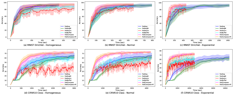
Figure 2: Change in validation accuracy and standard deviation for different FL algorithms on the dual Dirichlet partitioned MNIST dataset and the class partitioned CIFAR-10 dataset with five clients and three client heterogeneity settings. (Synchronous algorithms take the same amount of time and asynchronous algorithms take the same amount of time in the same experiment setting.)

Performance Comparison. Table 1 shows the relative wall-clock time for various FL algorithms to first reach the target validation accuracy on the partitioned MNIST and CIFAR-10 datasets with different numbers of clients and client heterogeneity settings. Table 2 reports the relative wall-clock time to reach 0.98 DICE accuracy (Dice, 1945) on the Fed-IXI dataset and 50% balanced accuracy on the Fed-ISIC2019 dataset in three heterogeneity settings. The numbers are the average results of ten runs with different random seeds, and the wall-clock time for FedCompass is used as a baseline. A dash “-” signifies that a certain algorithm cannot reach the target accuracy in at least half of the experiment runs. The dataset target accuracy is carefully selected based on each algorithm’s top achievable accuracy during training (given in Appendix F). Among the benchmarked algorithms, FedAvg (McMahan et al., 2017) is the most commonly used synchronous FL algorithm, and FedAvgM (Hsu et al., 2019) is a variant of FedAvg using server-side momentum to address non-IID data. FedAsync (Xie et al., 2019) and FedBuffer (Nguyen et al., 2022) are two popular asynchronous FL algorithms. As the Compass scheduler is separated from global aggregation, making FedCompass compatible with server-side optimization strategies, we also benchmark the performance of using server-side momentum in FedCompass (FedCompass+M). Tiered FL methods are omitted from our benchmarks since they either require prior knowledge of client computing power or are only relevant for cross-device FL, rendering them equivalent to FedAvg in a cross-silo FL context with only one cluster. From the table, we obtain the following key observations: (i) The speedup provided by asynchronous FL algorithms increases as client heterogeneity increases and synchronous FL algorithms have longer client idle times. (ii) Similar to synchronous FL where server-side optimizations can sometimes speed up the convergence, applying server momentum to FedCompass in group aggregation can sometimes speed up the convergence as well. This indicates that the design of FedCompass allows it to easily take advantage of other FL strategies. (iii) Due to client drift and model staleness, FedAsync and FedBuffer occasionally fail to achieve the target accuracy, particularly in settings with minimal client heterogeneity and unnecessary application of the staleness factor. On the other hand, FedCompass can quickly converge in all cases, as Compass dynamically and automatically groups clients for global aggregation, reducing client model staleness and mitigating the client drift problem. This shows that FedCompass outperforms other asynchronous algorithms on heterogeneous non-IID data without any prior knowledge of clients. Additionally, Figure 2 illustrates the change in validation accuracy during the training for different FL algorithms on the dual Dirichlet partitioned MNIST dataset (subplots a to c) and the class partitioned CIFAR-10 dataset (subplots d to f) with five clients and three client heterogeneity settings. In the plots, synchronous algorithms take the same amount of time, and asynchronous algorithms take the same amount of time in the same experiment setting. These plots further illustrate how FedCompass converges faster than other algorithms and also achieves higher accuracy than other asynchronous algorithms. For example, subplots d and e explicitly demonstrate that FedAsync and FedBuffer only converge to much lower accuracy in low-heterogeneity settings, mainly due to client drift from unnecessary staleness factors. More plots of the training process and the maximum achievable accuracy for each FL algorithm are given in Appendix F.

Effect of Number of Local Steps. We conduct ablation studies on the values of $\textit{1/Q}=Q_{\min}/Q_{\max}$ to investigate its impact on the performance of the FedCompass, with results listed in Table 3. From the table, we observe that smaller 1/Q values (ranging from 0.05 to 0.2) usually lead to faster convergence speed. Additionally, a wide range of 1/Q (ranging 0.05 from 0.8) can achieve a reasonable convergence rate compared with FedBuffer, which showcases that FedCompass is not sensitive to the value of Q. Therefore, users do not need to heuristically select Q for different client numbers and heterogeneity settings. In the extreme case that $\textit{Q}=1$, i.e. $Q_{\min}=Q_{\max}$, there is a significant performance drop for FedCompass, as Compass loses the flexibility to assign different local steps to different clients. Therefore, each client has its own arrival group and FedCompass becomes equivalent to FedAsync. More ablation study results are given in Appendix G.1.

Table 3: Relative wall-clock time for FedCompass to first reach the target validation accuracy on the dual Dirichlet partitioned MNIST datasets for various values of $\textit{1/Q}=Q_{\min}/Q_{\max}$.

Client number			$m=5$				$m=10$				$m=20$
Dataset	1/Q		homo	normal	exp		homo	normal	exp		homo	normal	exp
	0.05		0.89$\times$	1.01$\times$	0.85$\times$		0.96$\times$	0.97$\times$	0.82$\times$		1.00$\times$	1.02$\times$	0.96$\times$
	0.10		0.91$\times$	1.05$\times$	0.92$\times$		0.96$\times$	0.95$\times$	0.85$\times$		0.97$\times$	1.02$\times$	0.96$\times$
	0.20		1.00$\times$	1.00$\times$	1.00$\times$		1.00$\times$	1.00$\times$	1.00$\times$		1.00$\times$	1.00$\times$	1.00$\times$
MNIST-Dirichlet	0.40		1.02$\times$	1.03$\times$	1.70$\times$		1.04$\times$	1.05$\times$	1.28$\times$		1.00$\times$	1.14$\times$	1.25$\times$
Partition (90%)	0.60		1.04$\times$	1.01$\times$	1.83$\times$		1.00$\times$	1.01$\times$	1.19$\times$		0.92$\times$	1.11$\times$	1.16$\times$
	0.80		1.04$\times$	1.13$\times$	1.58$\times$		0.91$\times$	1.25$\times$	1.22$\times$		0.86$\times$	1.22$\times$	1.21$\times$
	1.00		1.78$\times$	1.68$\times$	2.01$\times$		-	2.28$\times$	1.29$\times$		-	-	1.76$\times$
FedBuffer			1.23$\times$	1.52$\times$	1.86$\times$		1.81$\times$	1.51$\times$	1.49$\times$		2.77$\times$	1.22$\times$	1.40$\times$

6 Conclusion

This paper introduces FedCompass, which employs a novel computing power aware scheduler to make several client models arrive almost simultaneously for group aggregation to reduce global aggregation frequency and mitigate the stale local model issues in asynchronous FL, thus enhancing the FL training efficiency with heterogeneous client devices, and improving the performance on non-IID heterogeneous distributed datasets. Through a comprehensive suite of experiments, we have demonstrated that FedCompass achieves faster convergence than other prevalent FL algorithms in various training tasks with heterogeneous training data and clients. This new approach opens up new pathways for the development and use of robust AI models in settings that require privacy, with the additional advantage that it can readily leverage the existing disparate computing ecosystem.

Reproducibility Statement

The source code and instructions to reproduce all the experiment results can be found in the supplemental materials. The details of the classic dataset partition strategies are provided in Appendix D, and the corresponding implementations are included in the source code. The setups and hyperparameters used in the experiments are given in Appendix E. Additionally, the proofs of Theorem 1 and Corollary 1 are provided in Appendix C.

Acknowledgments

The material is based upon work and resources of the Argonne Leadership Computing Facility at Argonne National Laboratory, which is supported by the U.S. Department of Energy, Office of Science, under contract number DE-AC02-06CH11357 and in part by MIDRC (The Medical Imaging and Data Resource Center) funded by the National Institutes of Health under contract 75N92020C00021. This research is also part of the Delta research computing project, which is supported by the National Science Foundation (award OCI 2005572), and the State of Illinois. Delta is a joint effort of the University of Illinois at Urbana-Champaign and its National Center for SuperComputing Applications.

Appendix A Detailed Implementation of FedCompass

Table 4 lists all frequently used notations and their corresponding explanations in the algorithm description of FedCompass.

Table 4: Summary of notations used in algorithm description of FedCompass.

Notation	Explanation
$\mathcal{C}$	client information dictionary
$\mathcal{G}$	arrival group information dictionary
$G$	index of the arrival group for a client
$Q$	number of local steps for a client
$S$	estimated computing speed for a client
$T_{\text{start}}$	start time of current local training round for a client
$CL$	list of non-arrived clients for an arrival group
$ACL$	list of arrived clients for an arrival group
$T_{a}$	expected arrival time for an arrival group
${T}_{\max}$	lastest arrival time for an arrival group
$T_{\text{now}}$	current time
$Q_{\max}$	maximum number of local steps for clients
$Q_{\min}$	minimum number of local steps for clients
$\lambda$	latest time factor
$\eta_{\ell}$	client learning rate
$N$	total number of communication rounds
$B$	batch size for local training
$st(\cdot)$	staleness function
$\tau$	timestamp of the global model that a client trained on
$\tau_{g}$	timestamp of the global model
$p_{i}$	importance weight of client $i$
$\Delta_{i}$	the difference between the original model and the trained model of client $i$
$\overline{\Delta}^{g}$	client update buffer for group $g$
$\overline{\Delta}$	general client update buffer
$w$	global model
$w_{i,q}$	local model of client $i$ after $q$ local steps

1

Function AssignGroup($i$): Input : Client id $i$

2 if $\textsc{JoinGroup}(i)=\texttt{False}$ then

3       $\textsc{CreateGroup}(i)$;

4      

5

6

Function JoinGroup($i$): Input : Client id $i$

7 Initialization: $G_{\text{assign}},Q_{\text{assign}}:=-1,-1$;

8 for $g\in\mathcal{G}$ do

9       $q:=\lfloor(\mathcal{G}\texttt{[}g\texttt{]}.T_{a}-T_{\text{now}})/\mathcal{C}\texttt{[}i\texttt{]}.S\rfloor$;

10       if $q\geq Q_{\min}$ and $q\geq Q_{\text{assign}}$ and $q\leq Q_{\max}$ then

11             $G_{\text{assign}},Q_{\text{assign}}:=g,q$;

12            

13      

14

15if $G_{\text{assign}}\neq-1$ then

16       $\mathcal{C}\texttt{[}i\texttt{]}.(G,Q,T_{\text{start}}):=(G_{\text{assign}},Q_{\text{assign}},T_{\text{now}})$;

17       $\mathcal{G}\texttt{[}g\texttt{]}.CL.\texttt{add(}i\texttt{)}$;

18       return True;

19      

20else

21       return False

22

23

Function CreateGroup($i$): Input : Client id $i$

24 Initialization: $Q_{\text{assign}}:=-1$;

25 for $g\in\mathcal{G}$ do

26       if $T_{\text{now}}<\mathcal{G}\texttt{[}g\texttt{]}.T_{a}$ then

27             $S:=\text{speed of the fastest client in group }g$;

28             $T_{\text{exp}}:=\mathcal{G}\texttt{[}g\texttt{]}.T_{a}+S*Q_{\max}$;

29             $Q_{\text{assign}}:=\max(Q_{\text{assign}},\lfloor(T_{\text{exp}}-T_{\text{now}})/\mathcal{C}\texttt{[}i\texttt{]}.S\rfloor)$;

30            

31      

32

33if $Q_{\text{assign}}\geq 0$ and $Q_{\text{assign}}<Q_{\min}$ then

34       $Q_{\text{assign}}:=Q_{\min}$;

35      

36else

37       if $Q_{\text{assign}}<0\ \texttt{or}\ Q_{\text{assign}}>Q_{\max}$ then

38             $Q_{\text{assign}}:=Q_{\max}$;

39            

40      

41

42$G_{\text{new}}:=\text{a unique id for the new group}$;

43 $\mathcal{G}\texttt{[}G_{\text{new}}\texttt{]}.(CL,ACL):=(\texttt{[}i\texttt{]},\texttt{[]})$;

44 $\mathcal{G}\texttt{[}G_{\text{new}}\texttt{]}.T_{a}:=T_{\text{now}}+Q_{\text{assign}}*\mathcal{C}\texttt{[}i\texttt{]}.S$;

45 $\mathcal{G}\texttt{[}G_{\text{new}}\texttt{]}.{T}_{\max}:=T_{\text{now}}+Q_{\text{assign}}*\mathcal{C}\texttt{[}i\texttt{]}.S*\lambda$;

46 $\mathcal{C}\texttt{[}i\texttt{]}.(G,Q,T_{\text{start}}):=(G_{\text{new}},Q_{\text{assign}},T_{\text{now}})$;

47 Add a timer event at $\mathcal{G}\texttt{[}G_{\text{new}}\texttt{]}.{T}_{\max}$ to invoke GroupAggregate($G_{\text{new}}$);

Algorithm 2 AssignGroup

1 Function GroupAggregate($g$):

Input: group index $g$

2 if $g\in\mathcal{G}$ then

3       $w:=w-\overline{\Delta}_{g}-\overline{\Delta}$;  $\overline{\Delta}:=\mathbf{0}$;  $\tau_{g}:=\tau_{g}+1$;

4       sort $\mathcal{G}\texttt{[}g\texttt{]}.ACL$ from fastest client to slowest client;

5       for $i\in\mathcal{G}\texttt{[}g\texttt{]}.ACL$ do

6             $\mathcal{C}\texttt{[}i\texttt{]}.\tau:=\tau_{g}$;

7             AssignGroup($i$) ;

8             FedCompass-Client($i$, $w$, $\mathcal{C}\texttt{[}i\texttt{]}.Q$, $\eta_{\ell}$, $B$);

9            

10      

Algorithm 3 GroupAggregate Algorithm

Compass utilizes the concept of arrival group to determine which clients are supposed to arrive together. To manage the client arrival groups, Compass employs two dictionaries: $\mathcal{C}$ for client information and $\mathcal{G}$ for arrival group information. Specifically, for client $i$, $\mathcal{C}\texttt{[}i\texttt{]}.G$, $\mathcal{C}\texttt{[}i\texttt{]}.Q$, $\mathcal{C}\texttt{[}i\texttt{]}.S$, and $\mathcal{C}\texttt{[}i\texttt{]}.T_{\text{start}}$ represent the arrival group, number of local steps, estimated computing speed (time per step), and start time of current communication round of client $i$. $\mathcal{C}\texttt{[}i\texttt{]}.\tau$ represents the timestamp of the global model upon which client $i$ trained (i.e., client local model timestamp). For arrival group $g$, $\mathcal{G}\texttt{[}g\texttt{]}.CL$, $\mathcal{G}\texttt{[}g\texttt{]}.ACL$, $\mathcal{G}\texttt{[}g\texttt{]}.T_{a}$, and $\mathcal{G}\texttt{[}g\texttt{]}.{T}_{\max}$ represent the list of non-arrived and arrived clients, expected arrival time for clients in the group, and latest arrival time for clients in the group. According to the client speed estimation, all clients in group $g$ are expected to finish local training and send the trained local updates back to the server before $\mathcal{G}\texttt{[}g\texttt{]}.T_{a}$, however, to account for potential errors in speed estimation and variations in computing speed, the group can wait until the latest arrival time $\mathcal{G}\texttt{[}g\texttt{]}.{T}_{\max}$ for the clients to send their trained models back. The difference between $\mathcal{G}\texttt{[}g\texttt{]}.{T}_{\max}$ and the group creation time is $\lambda$ times longer than the difference between $\mathcal{G}\texttt{[}g\texttt{]}.T_{a}$ and the group creation time.

Algorithm 2 presents the process through which Compass assigns a client to an arrival group. The dictionaries $\mathcal{C}$ and $\mathcal{G}$ along with the constant parameters $Q_{\max}$, $Q_{\min}$, and $\lambda$ are assumed to be available implicitly and are not explicitly passed as algorithm inputs. When Compass assigns a client to a group, it first checks whether it can join an existing arrival group (function JoinGroup, lines 5 to 16). For each group, Compass uses the current time, group expected arrival time, and estimated client speed to calculate a tentative local step number $q$ (line 8). To avoid large disparity in the number of local steps, Compass uses two parameters $Q_{\max}$ and $Q_{\min}$ to specify a valid range of local steps. If Compass can find the largest $q$ within the range $[Q_{\min},Q_{\max}]$, it assigns the client to the corresponding group. Otherwise, Compass creates a new arrival group for the client. When creating this new group, Compass aims to ensure that a specific existing arrival group can join the newly created group for group merging once all of its clients have arrived, as described in function CreateGroup (lines 18 to 35). To achieve this, Compass first identifies the computing speed $S$ of the fastest client in group $g$. It assumes that all clients in the group will arrive at the expected time $\mathcal{G}\texttt{[}g\texttt{]}.T_{a}$ and the fastest client will perform $Q_{\max}$ local steps in the next round. Subsequently, Compass utilizes the expected arrival time in the next round (line 23) to determine the appropriate number of local steps (line 24). It then selects the largest number of local steps while ensuring that it is within the range $[Q_{\min},Q_{\max}]$. In cases where Compass is unable to set the number of local steps in a way that allows any existing group to be suitable for joining in the next round, it assigns $Q_{\max}$ to the client upon creating the group. Whenever a new group is created, Compass sets up a timer event to invoke the GroupAggregate function (Algorithm 3) to aggregate the group of client updates after passing the group’s latest arrival time $\mathcal{G}\texttt{[}g\texttt{]}.T_{\max}$. In GroupAggregate, the server updates the global model using the group-specific buffer $\overline{\Delta}^{g}$, containing updates from clients in arrival group $g$, and the general buffer $\overline{\Delta}$, containing updates from clients arriving late in other groups. After the global update, the server updates the global model timestamp and assigns new training tasks to all arriving clients in group $g$.

Appendix B Upper Bound on the Number of Groups

If the client speeds do not have large variations for a sufficient number of global updates, then FedCompass can reach an equilibrium state where the arrival group assignment for clients is fixed and the total number of existing groups (denoted by $\#_{g}$) is bounded by $\lceil\log_{\textit{Q}}\mu\rceil$, where $\textit{Q}=Q_{\max}/Q_{\min}$ and $\mu$ is the ratio of the time per local step between the slowest client and the fastest client.

Consider one execution of FedCompass with a list of sorted client local computing times $\{\mathcal{T}_{1},\mathcal{T}_{2},\cdots,\mathcal{T}_{m}\}$ where $\mathcal{T}_{i}$ represents the time for client $i$ to complete one local step and $\mathcal{T}_{i}\leq\mathcal{T}_{j}$ if $i<j$. Let $\mathcal{G}_{1}=\{i\ |\ \frac{T_{i}}{T_{1}}\leq\frac{Q_{\max}}{Q_{\min}}\}=\{1,\cdots,g_{1}\}$ be the first group of clients, then all the clients $i\in\mathcal{G}_{1}$ will be assigned to the same arrival group at the equilibrium state with $Q_{i}=\frac{T_{1}}{T_{i}}Q_{\max}\in[Q_{\min},Q_{\max}]$. Similarly, if $g_{1}<m$, we can get the second group of clients $\mathcal{G}_{2}=\{i\ |\ \frac{T_{i}}{T_{g_{1}+1}}\leq\frac{Q_{\max}}{Q_{\min}}\}=\{g_{1}+1,\cdots,g_{2}\}$ where the clients in $\mathcal{G}_{2}$ will be assigned to another arrival group at the equilibrium state. Therefore, the maximum number of existing arrival groups at the equilibrium state is equal to the smallest integer such that

$$\Big{(}\frac{Q_{\max}}{Q_{\min}}\Big{)}^{\#_{g}}=\textit{Q}^{\#_{g}}\leq\frac{\mathcal{T}_{m}}{\mathcal{T}_{1}}=\mu\implies\#_{g}\leq\lceil\log_{\textit{Q}}\mu\rceil$$ (3)

Additionally, this implies that the maximum ratio of time for two different clients to finish one communication round at the equilibrium state is bounded by ${\mu}^{\prime}=\textit{Q}^{\lfloor\log_{\textit{Q}}\mu\rfloor}$. First, we can assume that the maximum ratio of time for two different clients to finish one communication round is the same as that for two different arrival groups to finish one communication round. In the extreme case that there are maximum $\lceil\log_{\textit{Q}}\mu\rceil$ arrival groups, then the time ratio between the slowest group and fastest group is then bounded by $\textit{Q}^{\lceil\log_{\textit{Q}}\mu\rceil-1}=\textit{Q}^{\lfloor\log_{\textit{Q}}\mu\rfloor}$.

Appendix C FedCompass Convergence Analysis

C.1 List of Notations

Table 5 lists frequently used notations in the convergence analysis of FedCompass.

Table 5: Frequently used notations in the convergence analysis of FedCompass.

Notation	Explanation
$m$	total number of clients
$\eta_{\ell}$	client local learning rate
$L$	Lipschitz constant
$\mu$	ratio of the time per local step between the slowest client and the fastest client
$\sigma_{l}$	bound for local gradient variance
$\sigma_{g}$	bound for global gradient variance
$M$	bound for gradient
$Q_{\min}$	minimum number of client local steps in each training round
$Q_{\max}$	maximum number of client local steps in each training round
Q	ratio between $Q_{\max}$ and $Q_{\min}$, i.e., $Q_{\max}/Q_{\min}$
$Q_{i,t}$	number of local steps for client $i$ in round $t$
$w^{(t)}$	global model after $t$ global updates
$w_{i,q}^{(t-\tau_{i,t})}$	local model of client $i$ after $q$ local steps, where the original model has timestamp $t-\tau_{i,t}$
$\mathcal{B}_{i,q}$	a random training batch that client $i$ uses in the $q$-th local step
$F(w)$	global loss for model $w$
$F_{i}(w)$	client $i$’s local loss for model $w$
$f_{i}(w,\mathcal{B}_{i})$	loss for model $w$ evaluated on batch $\mathcal{B}_{i}$ from client $i$
$\nabla F(w)$	gradient of global loss w.r.t. $w$
$\nabla F_{i}(w)$	gradient of client $i$’s local loss w.r.t. $w$
$\nabla f_{i}(w,\mathcal{B}_{i})$	gradient of loss evaluated on batch $\mathcal{B}_{i}$ w.r.t. $w$
$\mathcal{S}_{t}$	set of arriving clients at timestamp $t$
$\Delta_{i}^{(t-\tau_{i,t})}$	update from client $i$ at timestamp $t$ trained on global model with staleness $\tau_{i,t}$
$\overline{\Delta}^{(t)}$	aggregated local updates from clients for updating the global model at timestamp $t$

C.2 Proof of Theorem 1

Lemma 1.

$\mathbb{E}\Big{[}\|\nabla f_{i}(w,\mathcal{B}_{i})\|^{2}\Big{]}\leq 3(\sigma_{l}^{2}+\sigma_{g}^{2}+M)$ for any model $w$.

Proof of Lemma 1.

$$\mathbb{E}\Big{[}\|\nabla f_{i}(w,\mathcal{B}_{i})\|^{2}\Big{]}= \ \mathbb{E}\Big{[}\|\nabla f_{i}(w,\mathcal{B}_{i})-\nabla F_{i}(w)+\nabla F_{i}(w)-\nabla F(w)+\nabla F(w)\|^{2}\Big{]}$$ (4)

$$\overset{\text{(a)}}{\leq} \ 3\mathbb{E}\Big{[}\|\nabla f_{i}(w,\mathcal{B}_{i})-\nabla F_{i}(w)\|^{2}+\|\nabla F_{i}(w)-\nabla F(w)\|^{2}+\|\nabla F(w)\|^{2}\Big{]}$$

$$\overset{\text{(b)}}{\leq} \ 3(\sigma_{l}^{2}+\sigma_{g}^{2}+M),$$

where step (a) utilizes Cauchy-Schwarz inequality, and step (b) utilizes Assumption 3.

Lemma 2.

When a function $F:\mathbb{R}^{n}\rightarrow\mathbb{R}$ is Lipschitz smooth, then we have

$$F(w^{\prime})\leq F(w)+\langle\nabla F(w),w^{\prime}-w\rangle+\frac{L}{2}\|w^{\prime}-w\|^{2}\\$$ (5)

Proof of Lemma 2.

Let $w_{t}=w+t(w^{\prime}-w)$ for $t\in[0,1]$, then according to the definition of gradient, we have

$$F(w^{\prime})= \ F(w)+\int_{0}^{1}\langle\nabla F(w_{t}),w^{\prime}-w\rangle dt$$ (6)

$$= \ F(w)+\langle\nabla F(w),w^{\prime}-w\rangle+\int_{0}^{1}\langle\nabla F(w_{t})-\nabla F(w),w^{\prime}-w\rangle dt$$

$$\overset{\text{(a)}}{\leq} \ F(w)+\langle\nabla F(w),w^{\prime}-w\rangle+\int_{0}^{1}\|F(w_{t})-\nabla F(w)\|\cdot\|w^{\prime}-w\|dt$$

$$\overset{\text{(b)}}{\leq} \ F(w)+\langle\nabla F(w),w^{\prime}-w\rangle+L\int_{0}^{1}\|w_{t}-w\|\cdot\|w^{\prime}-w\|dt$$

$$= \ F(w)+\langle\nabla F(w),w^{\prime}-w\rangle+L\|w^{\prime}-w\|^{2}\int_{0}^{1}tdt$$

$$= \ F(w)+\langle\nabla F(w),w^{\prime}-w\rangle+\frac{L}{2}\|w^{\prime}-w\|^{2},$$

where step (a) utilizes Cauchy-Schwarz inequality $\langle u,v\rangle\leq|\langle u,v\rangle|\leq\|u\|\cdot\|v\|$, and step (b) utilizes the definition of Lipschitz smoothness.

Proof of Theorem 1.

According to Lemma 2, we have

$$F(w^{(t+1)}) \leq F(w^{(t)})+\langle\nabla F(w^{(t)}),w^{(t+1)}-w^{(t)}\rangle+\frac{L}{2}\|w^{(t+1)}-w^{(t)}\|^{2}$$ (7)

$$\leq F(w^{(t)})-\langle\nabla F(w^{(t)}),\overline{\Delta}^{(t)}\rangle+\frac{L}{2}\|\overline{\Delta}^{(t)}\|^{2}$$

$$=F(w^{(t)})\underbrace{-\frac{1}{m}\mathop{\sum}\limits_{k\in\mathcal{S}_{t}}\langle\nabla F(w^{(t)}),\Delta_{k}^{(t-\tau_{k,t})}\rangle}_{P_{1}}+\underbrace{\frac{L}{2m^{2}}\Big{\|}\mathop{\sum}\limits_{k\in\mathcal{S}_{t}}\Delta_{k}^{(t-\tau_{k,t})}\Big{\|}^{2}}_{P_{2}},$$

where $\mathcal{S}_{t}$ represents the set of clients arrived at timestamp $t$, and $\Delta_{k}^{(t-\tau_{k,t})}$ represents the update from client $k$ trained on global model with staleness $\tau_{k,t}$. Rearranging part $P_{1}$,

$$P_{1} =-\frac{1}{m}\mathop{\sum}\limits_{k\in\mathcal{S}_{t}}\langle\nabla F(w^{(t)}),\Delta_{k}^{(t-\tau_{k,t})}\rangle=-\frac{\eta_{\ell}}{m}\mathop{\sum}\limits_{k\in\mathcal{S}_{t}}\Big{\langle}\nabla F(w^{(t)}),\mathop{\sum}\limits_{q=0}^{Q_{k,t}-1}\nabla f_{k}(w_{k,q}^{(t-\tau_{k,t})},\mathcal{B}_{k,q})\Big{\rangle},$$ (8)

where $Q_{k,t}$ represents the number of local steps client $k$ has taken before sending the update to the server at timestamp $t$, $w_{k,q}^{(t-\tau_{k,t})}$ represents the model of client $k$ in local step $q$, and $\mathcal{B}_{k,q}$ represents a random training batch that the client $k$ uses in local step $q$. To compute an upper bound for the expectation of part $P_{1}$, we utilize conditional expectation: $\mathbb{E}[P_{1}]=\mathbb{E}_{\mathcal{H}}\mathbb{E}_{\{i\}\sim[m]|\mathcal{H}}\mathbb{E}_{\mathcal{B}_{i}|\{i\}\sim[m],\mathcal{H}}[P_{1}]$. Specifically, $\mathbb{E}_{\mathcal{H}}$ is the expectation over the history $\mathcal{H}$ of iterates up to timestamp $t$, $\mathbb{E}_{\{i\}\sim[m]|\mathcal{H}}$ is the expectation over the random group of clients arriving at timestamp $t$, and $\mathbb{E}_{\mathcal{B}_{i}|\{i\}\sim[m],\mathcal{H}}$ is the expectation over the mini-batch stochastic gradient on client $i$.

$$\mathbb{E}[P_{1}]= -\frac{\eta_{\ell}}{m}\mathbb{E}\Big{[}\mathop{\sum}\limits_{k\in\mathcal{S}_{t}}\Big{\langle}\nabla F(w^{(t)}),\mathop{\sum}\limits_{q=0}^{Q_{k,t}-1}\nabla f_{k}(w_{k,q}^{(t-\tau_{k,t})},\mathcal{B}_{k,q})\Big{\rangle}\Big{]}$$ (9)

$$\overset{\text{(a)}}{=} -\frac{\eta_{\ell}}{m}\mathbb{E}\Big{[}\mathop{\sum}\limits_{k\in\mathcal{S}_{t}}\mathop{\sum}\limits_{q=0}^{Q_{k,t}-1}\Big{\langle}\nabla F(w^{(t)}),\nabla F_{k}(w_{k,q}^{(t-\tau_{k,t})})\Big{\rangle}\Big{]},$$

$$\overset{\text{(b)}}{=} -\frac{\eta_{\ell}}{2m}\mathbb{E}\Big{[}\mathop{\sum}\limits_{k\in\mathcal{S}_{t}}\mathop{\sum}\limits_{q=0}^{Q_{k,t}-1}\Big{(}\|\nabla F(w^{(t)})\|^{2}-\|\nabla F(w^{(t)})-\nabla F_{k}(w_{k,q}^{(t-\tau_{k,t})})\|^{2}\Big{)}\Big{]}$$

$$-\frac{\eta_{\ell}}{2m}\mathbb{E}\Big{[}\mathop{\sum}\limits_{k\in\mathcal{S}_{t}}\mathop{\sum}\limits_{q=0}^{Q_{k,t}-1}\|\nabla F_{k}(w_{k,q}^{(t-\tau_{k,t})})\|^{2}\Big{]}$$

$$\overset{\text{(c)}}{=} -\frac{\eta_{\ell}}{2m}\mathbb{E}_{\mathcal{H}}\Big{[}\mathop{\sum}\limits_{i=1}^{m}\pi_{i}\mathop{\sum}\limits_{q=0}^{Q_{i,t}-1}\Big{(}\|\nabla F(w^{(t)})\|^{2}-\|\nabla F(w^{(t)})-\nabla F_{i}(w_{i,q}^{(t-\tau_{i,t})})\|^{2}\Big{)}\Big{]}$$

$$-\frac{\eta_{\ell}}{2m}\mathbb{E}\Big{[}\mathop{\sum}\limits_{k\in\mathcal{S}_{t}}\mathop{\sum}\limits_{q=0}^{Q_{k,t}-1}\|\nabla F_{k}(w_{k,q}^{(t-\tau_{k,t})})\|^{2}\Big{]}$$

$$= -\frac{\eta_{\ell}\mathcal{P}}{2m}\mathbb{E}_{\mathcal{H}}\Big{[}\mathop{\sum}\limits_{i=1}^{m}\pi_{i}^{\prime}\mathop{\sum}\limits_{q=0}^{Q_{i,t}-1}\|\nabla F(w^{(t)})\|^{2}\Big{]}$$

$$+\frac{\eta_{\ell}\mathcal{P}}{2m}\mathbb{E}_{\mathcal{H}}\Big{[}\mathop{\sum}\limits_{i=1}^{m}\pi_{i}^{\prime}\mathop{\sum}\limits_{q=0}^{Q_{i,t}-1}\|\nabla F(w^{(t)})-\nabla F_{i}(w_{i,q}^{(t-\tau_{i,t})})\|^{2}\Big{]}$$

$$-\frac{\eta_{\ell}}{2m}\mathbb{E}\Big{[}\mathop{\sum}\limits_{k\in\mathcal{S}_{t}}\mathop{\sum}\limits_{q=0}^{Q_{k,t}-1}\|\nabla F_{k}(w_{k,q}^{(t-\tau_{k,t})})\|^{2}\Big{]}$$

$$\leq -\frac{\eta_{\ell}}{2m}\mathbb{E}_{\mathcal{H}}\Big{[}\mathop{\sum}\limits_{i=1}^{m}\pi_{i}^{\prime}\mathop{\sum}\limits_{q=0}^{Q_{i,t}-1}\|\nabla F(w^{(t)})\|^{2}\Big{]}$$

$$+\frac{\eta_{\ell}}{2}\mathbb{E}_{\mathcal{H}}\Big{[}\mathop{\sum}\limits_{i=1}^{m}\pi_{i}^{\prime}\mathop{\sum}\limits_{q=0}^{Q_{i,t}-1}\|\nabla F(w^{(t)})-\nabla F_{i}(w_{i,q}^{(t-\tau_{i,t})})\|^{2}\Big{]}$$

$$-\frac{\eta_{\ell}}{2m}\mathbb{E}\Big{[}\mathop{\sum}\limits_{k\in\mathcal{S}_{t}}\mathop{\sum}\limits_{q=0}^{Q_{k,t}-1}\|\nabla F_{k}(w_{k,q}^{(t-\tau_{k,t})})\|^{2}\Big{]},$$

where step (a) utilizes Assumption 2, step (b) utilizes the identity $\langle u,v\rangle=\frac{1}{2}(\|u\|^{2}+\|v\|^{2}-\|u-v\|^{2})$, and step (c) utilizes conditional expectation with the probability $\pi_{i}$ of client $i$ to arrive at timestamp $t$. We let $\mathcal{P}=\mathop{\sum}\limits_{i=1}^{m}\pi_{i}\in[1,m]$ and $\pi_{i}^{\prime}:=\pi_{i}/\mathcal{P}$ such that $\mathop{\sum}\limits_{i=1}^{m}\pi_{i}^{\prime}=1$.

To derive the upper and lower bounds of $\pi_{i}^{\prime}$, according to the conclusion we get in Appendix B, we have $\pi_{\max}^{\prime}/\pi_{\min}^{\prime}\leq\textit{Q}^{\lfloor\log_{\textit{Q}}\mu\rfloor}=\mu^{\prime}$, i.e., $\pi_{\min}^{\prime}\geq\frac{1}{\mu^{\prime}}\pi_{\max}^{\prime}$. Therefore, we can derive the upper and lower bounds of $\pi_{i}^{\prime}$ as follows:

$$1=\mathop{\sum}\limits_{i=1}^{m}\pi_{i}^{\prime}\geq \pi_{\max}^{\prime}+(m-1)\pi_{\min}^{\prime}\geq\pi_{\max}^{\prime}+\frac{m-1}{\mu^{\prime}}\pi_{\max}^{\prime}$$ (10)

$$\pi_{\max}^{\prime}\leq\frac{1}{1+\frac{m-1}{\mu^{\prime}}}$$

$$1=\mathop{\sum}\limits_{i=1}^{m}\pi_{i}^{\prime}\leq \pi_{\min}^{\prime}+(m-1)\pi_{\max}^{\prime}\leq\pi_{\min}^{\prime}+\mu^{\prime}(m-1)\pi_{\min}^{\prime}$$ (11)

$$\pi_{\min}^{\prime}\geq\frac{1}{1+\mu^{\prime}(m-1)}$$

Let $\gamma_{1}=1+\frac{m-1}{\mu^{\prime}}$ and $\gamma_{2}=1+\mu^{\prime}(m-1)$, we have $\pi_{i}^{\prime}\in[\frac{1}{\gamma_{2}},\frac{1}{\gamma_{1}}]$. Then,

$$\mathbb{E}[P_{1}]\leq -\frac{\eta_{\ell}Q_{\min}}{2\gamma_{2}}\mathbb{E}\Big{[}\|\nabla F(w^{(t)})\|^{2}\Big{]}-\frac{\eta_{\ell}}{2m}\mathbb{E}\Big{[}\mathop{\sum}\limits_{k\in\mathcal{S}_{t}}\mathop{\sum}\limits_{q=0}^{Q_{k,t}-1}\|\nabla F_{k}(w_{k,q}^{(t-\tau_{k,t})})\|^{2}\Big{]}$$ (12)

$$+\underbrace{\frac{\eta_{\ell}}{2\gamma_{1}}\mathbb{E}_{\mathcal{H}}\Big{[}\mathop{\sum}\limits_{i=1}^{m}\mathop{\sum}\limits_{q=0}^{Q_{\max}-1}\|\nabla F(w^{(t)})-\nabla F_{i}(w_{i,q}^{(t-\tau_{i,t})})\|^{2}\Big{]}}_{P_{3}}$$

For part $P_{3}$, by utilizing Assumption 1, we can get

$$P_{3}= \ \frac{\eta_{\ell}}{2\gamma_{1}}\mathbb{E}_{\mathcal{H}}\Big{[}\mathop{\sum}\limits_{i=1}^{m}\mathop{\sum}\limits_{q=0}^{Q_{\max}-1}\|\nabla F(w^{(t)})-\nabla F_{i}(w_{i,q}^{(t-\tau_{i,t})})\|^{2}\Big{]}$$ (13)

$$\leq \ \frac{\eta_{\ell}}{\gamma_{1}}\mathbb{E}_{\mathcal{H}}\Big{[}\mathop{\sum}\limits_{i=1}^{m}\mathop{\sum}\limits_{q=0}^{Q_{\max}-1}\Big{(}\|\nabla F_{i}(w^{(t)})-\nabla F_{i}(w^{(t-\tau_{i,t})})\|^{2}+\|\nabla F_{i}(w^{(t-\tau_{i,t})})-\nabla F_{i}(w_{i,q}^{(t-\tau_{i,t})})\|^{2}\Big{)}\Big{]}$$

$$\leq \ \frac{\eta_{\ell}L^{2}}{\gamma_{1}}\mathbb{E}_{\mathcal{H}}\Big{[}\mathop{\sum}\limits_{i=1}^{m}\mathop{\sum}\limits_{q=0}^{Q_{\max}-1}\Big{(}\|w^{(t)}-w^{(t-\tau_{i,t})}\|^{2}+\|w^{(t-\tau_{i,t})}-w^{(t-\tau_{i,t})}_{i,q}\|^{2}\Big{)}\Big{]}$$

For $\|w^{(t)}-w^{(t-\tau_{i,t})}\|^{2}$, we derive its upper bound in the following way, with step (a) utilizing Cauchy-Schwarz inequality and step (b) utilizing Lemma 1.

$$\ \|w^{(t)}-w^{(t-\tau_{i,t})}\|^{2}=\Bigg{\|}\mathop{\sum}\limits_{\rho=t-\tau_{i,t}}^{t}(w^{(\rho+1)}-w^{(\rho)})\Bigg{\|}^{2}=\Bigg{\|}\mathop{\sum}\limits_{\rho=t-\tau_{i,t}}^{t}\frac{1}{m}\mathop{\sum}\limits_{k\in\mathcal{S}_{\rho}}\Delta_{k}^{(\rho-\tau_{k,\rho})}\Bigg{\|}^{2}$$ (14)

$$= \ \frac{\eta_{\ell}^{2}}{m^{2}}\Bigg{\|}\mathop{\sum}\limits_{\rho=t-\tau_{i,t}}^{t}\mathop{\sum}\limits_{k\in\mathcal{S}_{\rho}}\mathop{\sum}\limits_{q=0}^{Q_{k,\rho}-1}\nabla f_{k}(w_{k,q}^{(\rho-\tau_{k,\rho})},\mathcal{B}_{k,q})\Bigg{\|}^{2}$$

$$\overset{\text{(a)}}{\leq} \ \frac{\eta_{\ell}^{2}\tau_{\max}Q_{\max}}{m}\mathop{\sum}\limits_{\rho=t-\tau_{i,t}}^{t}\mathop{\sum}\limits_{k\in\mathcal{S}_{\rho}}\mathop{\sum}\limits_{q=0}^{Q_{k,\rho}-1}\Big{\|}\nabla f_{k}(w_{k,q}^{(\rho-\tau_{k,\rho})},\mathcal{B}_{k,q})\Big{\|}^{2}$$

$$\overset{\text{(b)}}{\leq} \ 3\eta_{\ell}^{2}\tau_{\max}^{2}Q_{\max}^{2}(\sigma_{l}^{2}+\sigma_{g}^{2}+M)$$

For $\|w^{(t-\tau_{i,t})}-w^{(t-\tau_{i,t})}_{i,q}\|^{2}$, we derive its upper bound also using Lemma 1.

$$\|w^{(t-\tau_{i,t})}-w^{(t-\tau_{i,t})}_{i,q}\|^{2}=\eta_{\ell}^{2}\Big{\|}\mathop{\sum}\limits_{e=0}^{q-1}\nabla f_{i}(w_{i,e}^{(t-\tau_{i,t})},\mathcal{B}_{i,e})\Big{\|}^{2}\leq 3\eta_{\ell}^{2}Q_{\max}^{2}(\sigma_{l}^{2}+\sigma_{g}^{2}+M)$$ (15)

Combining (14) and (15), we can obtain the upper bound of $P_{3}$:

$$P_{3}\leq\frac{3mL^{2}\eta_{\ell}^{3}Q_{\max}^{3}}{\gamma_{1}}(\tau_{\max}^{2}+1)(\sigma_{l}^{2}+\sigma_{g}^{2}+M)$$ (16)

Putting the upper bound of $P_{3}$ ((16)) into (12), we can get:

$$\mathbb{E}[P_{1}]\leq -\frac{\eta_{\ell}Q_{\min}}{2\gamma_{2}}\mathbb{E}\Big{[}\|\nabla F(w^{(t)})\|^{2}\Big{]}\underbrace{-\frac{\eta_{\ell}}{2m}\mathbb{E}\Big{[}\mathop{\sum}\limits_{k\in\mathcal{S}_{t}}\mathop{\sum}\limits_{q=0}^{Q_{k,t}-1}\|\nabla F_{k}(w_{k,q}^{(t-\tau_{k,t})})\|^{2}\Big{]}}_{P_{4}}$$ (17)

$$+\frac{3mL^{2}\eta_{\ell}^{3}Q_{\max}^{3}}{\gamma_{1}}(\tau_{\max}^{2}+1)(\sigma_{l}^{2}+\sigma_{g}^{2}+M)$$

To compute the upper bound for the expectation of part $P_{2}$, similar to $P_{1}$, we also apply conditional expectation: $\mathbb{E}[P_{2}]=\mathbb{E}_{\mathcal{H}}\mathbb{E}_{\{i\}\sim[m]|\mathcal{H}}[P_{2}]$.

$$\mathbb{E}[P_{2}]= \ \frac{L}{2m^{2}}\mathbb{E}\Bigg{[}\Big{\|}\mathop{\sum}\limits_{k\in\mathcal{S}_{t}}\Delta_{k}^{(t-\tau_{k,t})}\Big{\|}^{2}\Bigg{]}=\frac{\eta_{\ell}^{2}L}{2m^{2}}\mathbb{E}\Bigg{[}\Big{\|}\mathop{\sum}\limits_{k\in\mathcal{S}_{t}}\mathop{\sum}\limits_{q=0}^{Q_{k,t}-1}\nabla f_{k}(w_{k,q}^{(t-\tau_{k,t})},\mathcal{B}_{k,q})\Big{\|}^{2}\Bigg{]}$$ (18)

$$= \ \frac{\eta_{\ell}^{2}L}{2m^{2}}\mathbb{E}\Bigg{[}\Big{\|}\mathop{\sum}\limits_{k\in\mathcal{S}_{t}}\mathop{\sum}\limits_{q=0}^{Q_{k,t}-1}\Big{(}\nabla f_{k}(w_{k,q}^{(t-\tau_{k,t})},\mathcal{B}_{k,q})-\nabla F_{k}(w_{k,q}^{(t-\tau_{k,t})})\Big{)}+\mathop{\sum}\limits_{k\in\mathcal{S}_{t}}\mathop{\sum}\limits_{q=0}^{Q_{k,t}-1}\nabla F_{k}(w_{k,q}^{(t-\tau_{k,t})})\Big{\|}^{2}\Bigg{]}$$

$$\overset{\text{(a)}}{\leq} \ \frac{\eta_{\ell}^{2}L}{m^{2}}\mathbb{E}_{\mathcal{H}}\Bigg{[}\Big{\|}\mathop{\sum}\limits_{i=1}^{m}\pi_{i}\mathop{\sum}\limits_{q=0}^{Q_{i,t}-1}\Big{(}\nabla f_{i}(w_{i,q}^{(t-\tau_{i,t})},\mathcal{B}_{i,q})-\nabla F_{i}(w_{i,q}^{(t-\tau_{i,t})})\Big{)}\Big{\|}^{2}\Bigg{]}$$

$$+\frac{\eta_{\ell}^{2}L}{m^{2}}\mathbb{E}\Bigg{[}\Big{\|}\mathop{\sum}\limits_{k\in\mathcal{S}_{t}}\mathop{\sum}\limits_{q=0}^{Q_{k,t}-1}\nabla F_{k}(w_{k,q}^{(t-\tau_{k,t})})\Big{\|}^{2}\Bigg{]}$$

$$= \ \frac{\eta_{\ell}^{2}L\mathcal{P}^{2}}{m^{2}}\mathbb{E}_{\mathcal{H}}\Bigg{[}\Big{\|}\mathop{\sum}\limits_{i=1}^{m}\pi_{i}^{\prime}\mathop{\sum}\limits_{q=0}^{Q_{i,t}-1}\Big{(}\nabla f_{i}(w_{i,q}^{(t-\tau_{i,t})},\mathcal{B}_{i,q})-\nabla F_{i}(w_{i,q}^{(t-\tau_{i,t})})\Big{)}\Big{\|}^{2}\Bigg{]}$$

$$+\frac{\eta_{\ell}^{2}L}{m^{2}}\mathbb{E}\Bigg{[}\Big{\|}\mathop{\sum}\limits_{k\in\mathcal{S}_{t}}\mathop{\sum}\limits_{q=0}^{Q_{k,t}-1}\nabla F_{k}(w_{k,q}^{(t-\tau_{k,t})})\Big{\|}^{2}\Bigg{]}$$

$$\leq \ \frac{\eta_{\ell}^{2}L}{\gamma_{1}^{2}}\mathbb{E}_{\mathcal{H}}\Bigg{[}\Big{\|}\mathop{\sum}\limits_{i=1}^{m}\mathop{\sum}\limits_{q=0}^{Q_{i,t}-1}\Big{(}\nabla f_{i}(w_{i,q}^{(t-\tau_{i,t})},\mathcal{B}_{i,q})-\nabla F_{i}(w_{i,q}^{(t-\tau_{i,t})})\Big{)}\Big{\|}^{2}\Bigg{]}$$

$$+\frac{\eta_{\ell}^{2}L}{m^{2}}\mathbb{E}\Bigg{[}\Big{\|}\mathop{\sum}\limits_{k\in\mathcal{S}_{t}}\mathop{\sum}\limits_{q=0}^{Q_{k,t}-1}\nabla F_{k}(w_{k,q}^{(t-\tau_{k,t})})\Big{\|}^{2}\Bigg{]}$$

$$\overset{\text{(b)}}{\leq} \ \frac{m\eta_{\ell}^{2}LQ_{\max}}{\gamma_{1}^{2}}\mathop{\sum}\limits_{i=1}^{m}\mathop{\sum}\limits_{q=0}^{Q_{\max}-1}\mathbb{E}\Big{[}\Big{\|}\nabla f_{i}(w_{i,q}^{(t-\tau_{i,t})},\mathcal{B}_{i,q})-\nabla F_{i}(w_{i,q}^{(t-\tau_{i,t})})\Big{\|}^{2}\Big{]}$$

$$+\frac{\eta_{\ell}^{2}L}{m^{2}}\mathbb{E}\Bigg{[}\Big{\|}\mathop{\sum}\limits_{k\in\mathcal{S}_{t}}\mathop{\sum}\limits_{q=0}^{Q_{k,t}-1}\nabla F_{k}(w_{k,q}^{(t-\tau_{k,t})})\Big{\|}^{2}\Bigg{]}$$

$$\overset{\text{(c)}}{\leq} \ \frac{m^{2}\eta_{\ell}^{2}\sigma_{l}^{2}LQ_{\max}^{2}}{\gamma_{1}^{2}}+\underbrace{\frac{\eta_{\ell}^{2}L}{m^{2}}\mathbb{E}\Bigg{[}\Big{\|}\mathop{\sum}\limits_{k\in\mathcal{S}_{t}}\mathop{\sum}\limits_{q=0}^{Q_{k,t}-1}\nabla F_{k}(w_{k,q}^{(t-\tau_{k,t})})\Big{\|}^{2}\Bigg{]}}_{P_{5}},$$

where step (a) utilizes conditional expectation and Cauchy-Schwarz inequality, step (b) utilizes Caucht-Schwarz inequality, and step (c) utilizes the Assumption 3.

To find the upper bound of $\mathbb{E}[P_{1}+P_{2}]$, we need to make sure that $P_{4}+P_{5}\leq 0$ so that we can eliminate these two parts when evaluating the upper bound. The following step (a) employs Cauchy-Schwarz inequality.

$$P4+P5= -\frac{\eta_{\ell}}{2m}\mathbb{E}\Big{[}\mathop{\sum}\limits_{k\in\mathcal{S}_{t}}\mathop{\sum}\limits_{q=0}^{Q_{k,t}-1}\|\nabla F_{k}(w_{k,q}^{(t-\tau_{k,t})})\|^{2}\Big{]}+\frac{\eta_{\ell}^{2}L}{m^{2}}\mathbb{E}\Bigg{[}\Big{\|}\mathop{\sum}\limits_{k\in\mathcal{S}_{t}}\mathop{\sum}\limits_{q=0}^{Q_{k,t}-1}\nabla F_{k}(w_{k,q}^{(t-\tau_{k,t})})\Big{\|}^{2}\Bigg{]}$$ (19)

$$\overset{\text{(a)}}{\leq} -\frac{\eta_{\ell}}{2m}\mathbb{E}\Big{[}\mathop{\sum}\limits_{k\in\mathcal{S}_{t}}\mathop{\sum}\limits_{q=0}^{Q_{k,t}-1}\|\nabla F_{k}(w_{k,q}^{(t-\tau_{k,t})})\|^{2}\Big{]}+\frac{\eta_{\ell}^{2}LQ_{\max}}{m}\mathbb{E}\Bigg{[}\mathop{\sum}\limits_{k\in\mathcal{S}_{t}}\mathop{\sum}\limits_{q=0}^{Q_{k,t}-1}\Big{\|}\nabla F_{k}(w_{k,q}^{(t-\tau_{k,t})})\Big{\|}^{2}\Bigg{]}$$

$$= \ (\frac{\eta_{\ell}^{2}LQ_{\max}}{m}-\frac{\eta_{\ell}}{2m})\mathbb{E}\Big{[}\mathop{\sum}\limits_{k\in\mathcal{S}_{t}}\mathop{\sum}\limits_{q=0}^{Q_{k,t}-1}\|\nabla F_{k}(w_{k,q}^{(t-\tau_{k,t})})\|^{2}\Big{]}\leq 0$$

Therefore, we need to have $\eta_{\ell}\leq\frac{1}{2LQ_{\max}}$. In such cases, combining (17) and (18), we have

$$\mathbb{E}[F(w^{(t+1)})]\leq \ \mathbb{E}[F(w^{(t)})]-\frac{\eta_{\ell}Q_{\min}}{2\gamma_{2}}\mathbb{E}\Big{[}\|\nabla F(w^{(t)})\|^{2}\Big{]}+\frac{m^{2}\eta_{\ell}^{2}\sigma_{l}^{2}LQ_{\max}^{2}}{\gamma_{1}^{2}}$$ (20)

$$+\frac{3mL^{2}\eta_{\ell}^{3}Q_{\max}^{3}}{\gamma_{1}}(\tau_{\max}^{2}+1)(\sigma_{l}^{2}+\sigma_{g}^{2}+M)$$

Summing up $t$ from $0$ to $T-1$, we can get,

$$\frac{\eta_{\ell}Q_{\min}}{2\gamma_{2}}\mathop{\sum}\limits_{t=0}^{T-1}\mathbb{E}\Big{[}\|\nabla F(w^{(t)})\|^{2}\Big{]}\leq \mathop{\sum}\limits_{t=0}^{T-1}\Big{(}\mathbb{E}[F(w^{(t)})]-\mathbb{E}[F(w^{(t+1)})]\Big{)}+\frac{m^{2}\eta_{\ell}^{2}\sigma_{l}^{2}LQ_{\max}^{2}T}{\gamma_{1}^{2}}$$ (21)

$$+\frac{3mL^{2}\eta_{\ell}^{3}Q_{\max}^{3}T}{\gamma_{1}}(\tau_{\max}^{2}+1)(\sigma_{l}^{2}+\sigma_{g}^{2}+M)$$

$$\leq \ \Big{(}F(w^{(0)})-F(w^{*})\Big{)}+\frac{m^{2}\eta_{\ell}^{2}\sigma_{l}^{2}LQ_{\max}^{2}T}{\gamma_{1}^{2}}$$

$$+\frac{3mL^{2}\eta_{\ell}^{3}Q_{\max}^{3}T}{\gamma_{1}}(\tau_{\max}^{2}+1)(\sigma_{l}^{2}+\sigma_{g}^{2}+M)$$

Therefore, we obtain the conclusion in Theorem 1.

$$\frac{1}{T}\mathop{\sum}\limits_{t=0}^{T-1}\mathbb{E}\Big{[}\|\nabla F(w^{(t)})\|^{2}\Big{]}\leq \frac{2\gamma_{2}\Big{(}F(w^{(0)})-F(w^{*})\Big{)}}{\eta_{\ell}Q_{\min}T}+\frac{2\gamma_{2}\eta_{\ell}m^{2}\sigma_{l}^{2}LQ_{\max}^{2}}{\gamma_{1}^{2}Q_{\min}}$$ (22)

$$+\frac{6\gamma_{2}m\eta_{\ell}^{2}L^{2}Q_{\max}^{3}}{\gamma_{1}Q_{\min}}(\tau_{\max}^{2}+1)(\sigma_{l}^{2}+\sigma_{g}^{2}+M)$$

Proof of Corollary 1.

When $Q_{\min}\leq{Q_{\max}}/{\mu}$, then $\mu\leq Q_{\max}/Q_{\min}=\textit{Q}$. Therefore,

$$\mu^{\prime}=\textit{Q}^{\lfloor\log_{\textit{Q}}\mu\rfloor}=\textit{Q}^{0}=1$$ (23)

Consequently, $\gamma_{1}=1+\frac{m-1}{\mu^{\prime}}=m,\gamma_{2}=1+\mu^{\prime}(m-1)=m$. Letting $F^{*}=F(w^{(0)})-F(w^{*})$, and $\sigma^{2}=\sigma_{l}^{2}+\sigma_{g}^{2}+M$, (22) can be written as

$$\frac{1}{T}\mathop{\sum}\limits_{t=0}^{T-1}\mathbb{E}\Big{[}\|\nabla F(w^{(t)})\|^{2}\Big{]}\leq \frac{2mF^{*}}{\eta_{\ell}Q_{\min}T}+\frac{2\eta_{\ell}m\sigma_{l}^{2}LQ_{\max}^{2}}{Q_{\min}}+\frac{6m\eta_{\ell}^{2}\sigma^{2}L^{2}Q_{\max}^{3}}{Q_{\min}}(\tau_{\max}^{2}+1)$$ (24)

If choosing $\eta_{\ell}=\mathcal{O}(1/Q_{\max}\sqrt{T})$ and considering $Q_{\max}$ and $Q_{\min}$ having the same order in the $\mathcal{O}$-class estimation, we can derive the conclusion of Corollary 1.

$$\underset{t\in[T]}{\min}\ \mathbb{E}\|\nabla F(w^{(t)})\|^{2}\leq\frac{1}{T}\mathop{\sum}\limits_{t=0}^{T-1}\mathbb{E}\Big{[}\|\nabla F(w^{(t)})\|^{2}\Big{]}\leq \mathcal{O}\Big{(}\frac{mF^{*}}{\sqrt{T}}\Big{)}+\mathcal{O}\Big{(}\frac{m\sigma_{l}^{2}L}{\sqrt{T}}\Big{)}+\mathcal{O}\Big{(}\frac{m\tau_{\max}^{2}\sigma^{2}L^{2}}{T}\Big{)}$$ (25)

Appendix D Details of the Experiment Datasets

D.1 Classic Dataset Partition Strategy

To simulate data heterogeneity on the classic datasets, we employ two partition strategies: (i) class partition and (ii) dual Dirichlet partition, and apply them to both the MNIST (LeCun, 1998) and CIFAR-10 (Krizhevsky et al., 2009) datasets. The details of these two partition strategies are elaborated in the following subsections.

D.1.1 Class Partition

Data: Classic dataset $\mathcal{D}$, sample indices for different classes $class\_indices$, number of clients $m$, total number of distinct classes $n$, minimum and maximum number of sample classes for each client split $n_{\min}$ and $n_{\max}$, mean value of the normal distribution $\mu$, standard deviation of the normal distribution $\sigma$.

1 $client\_datasets:=\{i:\texttt{[]}\textbf{ for }i\in[1,m]\}$ $\ \triangleright$ Return value: local datasets for each client;

2 repeat

3       $class\_partition:=\{\}$ $\ \triangleright$ For a certain class, which client(s) have samples of that class in its own client split;

4       for $i\in[1,m]$ do

5             $n_{i}:=\texttt{randint(}n_{\min},n_{\max}\texttt{)}$;

6             $classes_{i}:=\texttt{randpermutation(}n\texttt{)[:}n_{i}\texttt{]}$;

7             for $c\in classes_{i}$ do

8                   $class\_partition[c]:=\texttt{[}i\texttt{]}\textbf{ if }c\notin class\_partition\textbf{ else }class\_partition\texttt{[}c\texttt{]}.add(i)$;

9                  

10            

11      

12until $\texttt{len(}class\_partition\texttt{)}=n$;

13for $c\in class\_partition$ do

14       $n_{s}:=\texttt{normal(mean=}\mu,\texttt{std=}\sigma,\texttt{size=}\texttt{len(}class\_partition\texttt{[}c\texttt{]}\texttt{)}\texttt{)}$;

15       $n_{s}:=(n_{s}/\texttt{sum(}n_{s}\texttt{)})*\texttt{len(}class\_indices\texttt{[}c\texttt{]}\texttt{)}$ $\ \triangleright$ Number of samples with class $c$ for each assigned client;

16       for $num,i\in\texttt{zip(}n_{s},class\_partition\texttt{[}c\texttt{]}\texttt{)}$ do

17             Add $num$ samples of $\mathcal{D}$ with distinct indices from $classes\_indices\texttt{[}c\texttt{]}$ to $client\_datasets\texttt{[}i\texttt{]}$;

18            

19      

20return $client\_datasets$;

Algorithm 4 ClassPartition

Algorithm 4 outlines the process of class partition, which partitions a classic dataset into several client splits such that each client split only has samples from a few classes. Many previous research works partition the classical dataset in a similar way to artificially create non-IID federated datasets (McMahan et al., 2017; Chen et al., 2019). To partition a dataset $\mathcal{D}$, we first obtain a dictionary $class\_indices$ which contains the indices of samples belonging to each class. Namely, $class\_indices\texttt{[}c\texttt{]}$ represents the indices of all samples in $\mathcal{D}$ with class $c$. Lines 2 to 9 of the algorithm assign each client $i$ with $n_{i}$ classes for its own client split, where $n_{i}\in[n_{\min},n_{\max}]$. Additionally, the algorithm ensures that each sample class is assigned to at least one client split. Subsequently, from lines 10 to 14, the algorithm determines the number of samples of class $c$ that each assigned client split should have based on a normal distribution, and then assigns the corresponding number of data samples to the respective clients. The class partition strategy results in imbalanced and non-IID FL datasets, with clients having varying sample classes within their local datasets.

In the experiments, the mean value of the normal distribution $\mu=10$, and the standard deviation $\sigma=3$. Both the MNIST and the CIFAR-10 datasets have 10 distinct classes, i.e., $n=10$. When the number of clients $m=5$, $n_{\min}=5$ and $n_{\max}=6$, when $m=10$ or $20$, $n_{\min}=3$ and $n_{\max}=5$. Figure 3 shows a sample class distribution generated by the class partition strategy among $m=10$ clients with $n_{\min}=3$, $n_{\max}=5$, and $n=10$.

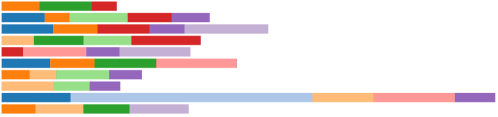
Figure 3: Sample class distribution generated by the class partition strategy among ten clients.

D.1.2 Dual Dirichlet Partition

Data: Classic dataset $\mathcal{D}$, sample indices for different classes $class\_indices$, number of clients $m$, total number of distinct classes $n$, two concentration parameters $\alpha_{1}$ and $\alpha_{2}$ for Dirichlet distributions.

1 $client\_datasets:=\{i:\texttt{[]}\textbf{ for }i\in[1,m]\}$ $\ \triangleright$ Return value: local datasets for each client;

2 $\mathbf{p_{1}}:=\texttt{[}1/m\textbf{ for }i\in[1,m]\texttt{]}$ $\ \triangleright$ Prior distribution for the number of samples for each client;

3 $\mathbf{p_{2}}:=\texttt{[len(}class\_indices\texttt{[}c\texttt{]}\texttt{)}\textbf{ for }c\in class\_indices$];

4 $\mathbf{p_{2}}:=\texttt{[}p/\texttt{sum(}\mathbf{p_{2}}\texttt{)}\textbf{ for }p\in\mathbf{p_{2}}\texttt{]}$ $\triangleright$ Prior distribution for the number of samples for each class;

5 $\boldsymbol{\alpha_{1}}:=\alpha_{1}*\mathbf{p_{1}}$;

6 $\boldsymbol{\alpha_{2}}:=\alpha_{2}*\mathbf{p_{2}}$;

7 $client\_wts:=\texttt{dirichlet(}\boldsymbol{\alpha_{1}}\texttt{)}$ $\ \triangleright$ Normalized number of samples for each client, shape is $\mathbb{R}^{m}$, sum is 1;

8 $class\_wts:=\texttt{dirichlet(}\boldsymbol{\alpha_{2}},\texttt{size=}m\texttt{)}$ $\ \triangleright$ Normalized number of samples for each class within each client, shape is $\mathbb{R}^{m\times n}$, row sum is 1;

9 for $i\in[1,m]$ do

10       for $c\in[1,n]$ do

11             $num:=client\_wts[i]*class\_wts[i][c]*\texttt{len(}class\_indices[c])/\langle client\_wts,class\_wts[:,c]\rangle$;

12             Add $num$ samples of $\mathcal{D}$ with distinct indices from $classes\_indices\texttt{[}c\texttt{]}$ to $client\_datasets\texttt{[}i\texttt{]}$;

13            

14      

15return $client\_datasets$;

Algorithm 5 DualDirichletPartition

Some prior works that model data heterogeneity also employ a Dirichlet distribution to model the class distribution within each local client dataset (Yurochkin et al., 2019; Hsu et al., 2019). We extend the work of others using two Dirichlet distributions with details outlined in Algorithm 5. The first Dirichlet distribution uses concentration parameter $\alpha_{1}$ and prior distribution $\mathbf{p_{1}}$ to generate the normalized number of samples for each client, $client\_wts\in\mathbb{R}^{m}$. The second Dirichlet distribution uses concentration parameter $\alpha_{2}$ and prior distribution $\mathbf{p_{2}}$ to generate the normalized number of samples for each class within each client, $class\_wts\in\mathbb{R}^{m\times n}$. From lines 9 to 12, the algorithm combines $client\_wts$, $class\_wts$, and the total number of samples for class $c$ to calculate the number of samples with class $c$ to be assigned for each client, and assigns the samples accordingly. In summary, the dual Dirichlet partition strategy employs two Dirichlet distributions to model two levels of data heterogeneity: the distribution across clients and the distribution across different classes within each client. Therefore, the generated client datasets are imbalanced and non-IID, which more accurately reflect real world federated datasets.

In the experiments, we set $\alpha_{1}=m$ and $\alpha_{2}=0.5$. The concentration parameter $\alpha$ governs the similarity among clients or classes. When $\alpha\rightarrow\infty$, the distribution becomes identical to the prior distribution. Conversely, when $\alpha\rightarrow 0$, only one item is selected with a value of 1 while the remaining items have a value of 0. As concentration parameter $\alpha_{2}$ has a very small value, each client only has data samples from a few classes. Figure 4 illustrates a sample class distribution generated by the dual Dirichlet partition strategy among $m=10$ clients, where $n=10$, $\alpha_{1}=10$, and $\alpha_{2}=0.5$.

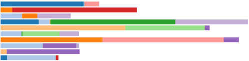
Figure 4: Sample class distribution generated by the dual Dirichlet partition strategy among ten clients.

D.2 Naturally Split Datasets: FLamby

FLamby is an open-source suite that provides naturally split datasets specifically designed for benchmarking cross-silo federated learning algorithms (Ogier du Terrail et al., 2022). These datasets are sourced directly from distributed real-world entities, ensuring that they preserve the authentic characteristics and complexities of data distribution in FL. In our study, we selected two medium-sized datasets from FLamby – Fed-IXI, and Fed-ISIC2019 – to evaluate the performance of FedCompass and other FL algorithms in the experiments. The two datasets offer valuable perspectives into two healthcare domains, brain MRI interpretation (Fed-IXI), and skin cancer detection (Fed-ISIC2019). By leveraging these datasets, our goal is to showcase the robustness and versatility of FedCompass across diverse machine learning tasks in real-world scenarios. Table 6 provides the overview of the two selected datasets in FLamby. Detailed descriptions of these datasets are provided in the following subsections.

Table 6: Overview of the two selected datasets in FLamby.

Dataset	Fed-IXI	Fed-ISIC2019
Inputs	T1 weighted image (T1WI)	Dermoscopy
Task type	3D segmentation	Classification
Prediction	Brain mask	Melanoma class
Client number	3	6
Model	3D U-net(Çiçek et al., 2016)	EfficientNet(Tan & Le, 2019)
Metric	DICE (Dice, 1945)	Balanced accuracy
Input dimension	48 $\times$ 60 $\times$ 48	200 $\times$ 200 $\times$ 3
Dataset size	444MB	9GB

D.2.1 Fed-IXI

Fed-IXI dataset is sourced from the Information eXtraction from Images (IXI) database and includes brain T1 magnetic resonance images (MRIs) from three hospitals (Pérez-García et al., 2021). These MRIs have been repurposed for a brain segmentation task; the model performance is evaluated with the DICE score (Dice, 1945). To ensure consistency, the images undergo preprocessing steps like volume resizing to 48 × 60 × 48 voxels, and sample-wise intensity normalization. The 3D U-net (Çiçek et al., 2016) serves as the baseline model for this task.

D.2.2 Fed-ISIC2019

Fed-ISIC2019 dataset is sourced from the ISIC2019 dataset, which includes dermoscopy images collected from four hospitals (Tschandl et al., 2018; Codella et al., 2018; Combalia et al., 2019). The images are restricted to a subset from the public train set and are split based on the imaging acquisition system, resulting in a 6-client federated dataset. The task involves image classification among eight different melanoma classes, and the performance is measured through balanced accuracy. Images are preprocessed by resizing and normalizing brightness and contrast. The baseline classification model is an EfficientNet (Tan & Le, 2019) pretrained on ImageNet (Deng et al., 2009).

Appendix E Experiment Setup Details

All the experiments are implemented using the open-source software framework for privacy-preserving federated learning (Ryu et al., 2022; Li et al., 2023).

E.1 Details of Client Heterogeneity Simulation

When simulating the client heterogeneity, we consider the average time $t_{i}$ required for client $i$ to complete one local step. We assume that $t_{i}$ follows a random distribution $P$, i.e. $t_{i}\sim P(t)$. In our experiments, we employ three different distributions to simulate client heterogeneity: the normal distribution $t_{i}\sim\mathcal{N}(\mu,\sigma^{2})$ with $\sigma=0$ (i.e., homogeneous clients), the normal distribution $t_{i}\sim\mathcal{N}(\mu,\sigma^{2})$ with $\sigma=0.3\mu$, and the exponential distribution $t_{i}\sim\textit{Exp}(\lambda)$. The exponential distribution models the amount of time until a certain event occurs (arrival time), specifically events that follow a Poisson process. The mean values of the distribution ($\mu$ or $1/\lambda$) are adjusted for different datasets according to the size of the model and training data. Table 7 presents the mean values of the client training time distribution for different datasets used in the experiments. Furthermore, Figure 5 illustrates the distribution of the training time to complete one local step among 50 clients under normal distribution with $\sigma=0.3\mu$ and exponential distribution, both with a mean value of 0.15.

Table 7: Mean values of the training time distribution for different datasets.

Dataset Name	Batch Size	Mean ($\mu$ or $1/\lambda$)
MNIST	64	0.15s
CIFAR-10	128	0.5s
Fed-IXI	2	0.8s
Fed-ISIC2019	64	1.5s

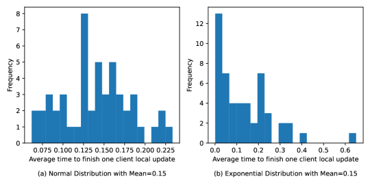
Figure 5: A sample distribution of the training time to complete one local step among 50 clients under (a) normal distribution with $\sigma=0.3\mu$, and (b) exponential distribution.

E.2 Detailed Setups and Hyperparameters for Experiments on the MNIST Dataset

Table 8 shows the detailed architecture of the convolutional neural network (CNN) used for the experiments on the MNIST dataset. Table 9 provides a comprehensive list of the hyperparameter values used for training. Specifically, $Q$ is the number of client local steps for each training round, $Q_{\min}$ and $Q_{\max}$ are the minimum and maximum numbers of client local steps in FedCompass, $\eta_{\ell}$ is the client local learning rate, $\beta$ is the server-side momentum, and $B$ is the batch size. For all asynchronous FL algorithms, we adopt the polynomial staleness function introduced in (Xie et al., 2019), denoted as $st(t-\tau)=\alpha(t-\tau+1)^{-a}$. The values of $\alpha$ and $a$ are also listed in Table 9 for all asynchronous algorithms. Additionally, $K$ is the buffer size for the FedBuffer algorithm, and $\lambda$ is the latest time factor for FedCompass. For hyperparameters given as length-three tuples, the tuple items correspond to the hyperparameter values when the number of clients is 5, 10, and 20, respectively. For hyperparameters that are not applicable to certain algorithms, the corresponding value is marked as a dash “-”. To ensure a fair comparison, similar algorithms are assigned the same hyperparameter values, as depicted in the table. The number of global training rounds is chosen separately for different experiment settings and FL algorithms such that the corresponding FL algorithm converges, synchronous FL algorithms take the same amount of wall-clock time and asynchronous algorithms take the same amount of wall-clock time in the same setting.

Table 8: MNIST CNN model architecture.

Layer	Outsize	Setting	Parama #
Input	(1, 28, 28)	-	0
Conv1	(32, 24, 24)	kernel=5, stride=1	832
ReLU1	(32, 24, 24)	-	0
MaxPool1	(32, 12, 12)	kernel=2, stride=2	0
Conv2	(64, 8, 8)	kernel=5, stride=1	51,264
ReLU2	(64, 8, 8)	-	0
MaxPool2	(64, 4, 4)	kernel=2, stride=2	0
Flatten	(1024,)	-	0
FC1	(512,)	-	524,800
ReLU2	(512,)	-	0
FC2	(10,)	-	5,130

Table 9: Hyperparameters for various FL algorithms on the MNIST dataset.

	FedAvg	FedAvgM	FedAsync	FedBuffer	FedCompass	FedCompass+M
$Q$	(200, 200, 100)	(200, 200, 100)	(200, 200, 100)	(200, 200, 100)	-	-
$Q_{\min}$	-	-	-	-	(40, 40, 20)	(40, 40, 20)
$Q_{\max}$	-	-	-	-	(200, 200, 100)	(200, 200, 100)
Optimizer	Adam	Adam	Adam	Adam	Adam	Adam
$\eta_{\ell}$	0.003	0.003	0.003	0.003	0.003	0.003
$\beta$	-	0.9	-	-	-	0.9
$B$	64	64	64	64	64	64
$\alpha$	-	-	0.9	0.9	0.9	0.9
$a$	-	-	0.5	0.5	0.5	0.5
$K$	-	-	-	(3, 3, 5)	-	-
$\lambda$	-	-	-	-	1.2	1.2

E.3 Detailed Setups and Hyperparameters for Experiments on the CIFAR-10 Dataset

For experiments on the CIFAR-10 dataset, a randomly initialized ResNet-18 model (He et al., 2016) is used in training. Table 10 shows the detailed architecture of the ResNet-18 model, which contains eight residual blocks. Each residual block contains two convolutional + batch normalization layers, as shown in Table 11, and the corresponding output is added by the input itself if the output channel is equal to the input channel, otherwise, the input goes through a 1x1 convolutional + batch normalization layer before adding to the output. An additional ReLU layer is appended at the end of the residual block. Table 12 lists the hyperparameter values used in the training for various FL algorithms. The number of global training rounds is chosen separately for different experiment settings and FL algorithms such that the corresponding FL algorithm converges, synchronous FL algorithms take the same amount of wall-clock time and asynchronous algorithms take the same amount of wall-clock time in the same setting.

Table 10: CIFAR-10 ResNet18 model architecture.

Layer	Outsize	Setting	Param #
Input	(3, 32, 32)	-	0
Conv1	(64, 32, 32)	kernel=3, stride=1, padding=1, bias=False	1,728
BatchNorm1	(64, 32, 32)	-	128
ReLU1	(64, 32, 32)	-	0
ResidualBlock1-1	(64, 32, 32)	stride=1	73,984
ResidualBlock1-2	(64, 32, 32)	stride=1	73,984
ResidualBlock2-1	(128, 16, 16)	stride=2	230,144
ResidualBlock2-2	(128, 16, 16)	stride=1	295,424
ResidualBlock3-1	(256, 8, 8)	stride=2	919,040
ResidualBlock3-2	(256, 8, 8)	stride=1	1,180,672
ResidualBlock4-1	(512, 4, 4)	stride=2	3,673,088
ResidualBlock4-2	(512, 4, 4)	stride=1	4,720,640
AvgPool	(512,)	kernel=4, stride=4	0
Linear	(10,)	-	5,130

Table 11: ResidualBlock in ResNet18 architecture.

Layer	Outsize	Setting	Param #
Input	(in_planes, H, W)	-	0
Conv1	(planes, H/stride, W/stride)	kernel=3, stride=stride, padding=1	in_planes*planes*9
BatchNorm1	(planes, H/stride, W/stride)	-	2*planes
ReLU1	(planes, H/stride, W/stride)	-	0
Conv2	(planes, H/stride, W/stride)	kernel=3, stride=1, padding=1	planes*planes*9
BatchNorm2	(planes, H/stride, W/stride)	-	2*planes
“Identity”	(planes, H/stride, W/stride)	1x1 Conv + BatchNorm if in_plane $\neq$ plane	-
ReLU2	(planes, H/stride, W/stride)	$\triangleright$ Apply after adding BatchNorm2 and “Identity” outputs	0

Table 12: Hyperparameters for various FL algorithms on the CIFAR-10 dataset.

	FedAvg	FedAvgM	FedAsync	FedBuffer	FedCompass	FedCompass+M
$Q$	(200, 200, 100)	(200, 200, 100)	(200, 200, 100)	(200, 200, 100)	-	-
$Q_{\min}$	-	-	-	-	(40, 40, 20)	(40, 40, 20)
$Q_{\max}$	-	-	-	-	(200, 200, 100)	(200, 200, 100)
Optimizer	SGD	SGD	SGD	SGD	SGD	SGD
$\eta_{\ell}$	0.1	0.1	0.1	0.1	0.1	0.1
$\beta$	-	0.9	-	-	-	0.9
$B$	128	128	128	128	128	128
$\alpha$	-	-	0.9	0.9	0.9	0.9
$a$	-	-	0.5	0.5	0.5	0.5
$K$	-	-	-	(3, 3, 5)	-
$\lambda$	-	-	-	-	1.2	1.2

E.4 Detailed Setups and Hyperparameters for Experiments on the FLamby Datasets

For the datasets from FLamby (Ogier du Terrail et al., 2022), we use the default experiments settings provided by FLamby. The details of the experiment settings are shown in Table 13

Table 13: Detailed settings for experiments on FLamby datasets.

	Fed-IXI	Fed-ISIC2019
Model	3D U-net (Çiçek et al., 2016)	EfficientNet (Tan & Le, 2019)
Metric	DICE	Balanced accuracy
$m$ (Client #)	3	6
$Q$	50	50
$Q_{\min}$	20	20
$Q_{\max}$	100	100
Optimizer	AdamW (Loshchilov & Hutter, 2017)	Adam
$\eta_{\ell}$	0.001	0.0005
$\beta$	0.9	0.5
$B$	2	64
$\alpha$	0.9	0.9
$a$	0.5	0.5
$K$	2	3
$\lambda$	1.2	1.2

Appendix F Additional Experiment Results

F.1 Additional Experiment Results on the MNIST Dataset

Table 14 shows the top validation accuracy and the corresponding standard deviation on the class partitioned MNIST dataset for various federated learning algorithms with different numbers of clients and client heterogeneity settings among ten independent experiment runs with different random seeds, and Table 15 shows that on the dual Dirichlet partitioned MNIST dataset. As all asynchronous FL algorithms take the same amount of training time in the same experiment setting, the results indicate that FedCompass not only converges faster than other asynchronous FL algorithms, but it can also converge to higher accuracy.

Figures 6 to 11 depict the change in validation accuracy during the training process for various FL algorithms in different experiment settings. Those figures illustrate how FedCompass can achieve faster convergence in different data and device heterogeneity settings.

Table 14: Average top validation accuracy and standard deviation on the class partitioned MNIST dataset for various federated learning algorithms with different numbers of clients and client heterogeneity settings.

		$n=5$				$n=10$				$n=20$
Method		homo	normal	exp		homo	normal	exp		homo	normal	exp
FedAvg		92.42$\pm$3.96	92.42$\pm$3.96	92.42$\pm$3.96		92.27$\pm$3.88	92.27$\pm$3.88	92.27$\pm$3.88		97.38$\pm$1.59	97.38$\pm$1.59	97.38$\pm$1.59
FedAvgM		96.22$\pm$2.45	96.22$\pm$2.45	96.22$\pm$2.45		97.11$\pm$1.45	97.11$\pm$1.45	97.11$\pm$1.45		98.27$\pm$0.18	98.27$\pm$0.18	98.27$\pm$0.18
FedAsync		90.60$\pm$6.96	92.53$\pm$5.57	92.44$\pm$3.07		86.73$\pm$6.62	92.27$\pm$3.82	96.25$\pm$2.46		84.26$\pm$7.96	90.98$\pm$2.48	98.01$\pm$0.89
FedBuffer		95.77$\pm$1.93	94.69$\pm$3.52	95.68$\pm$1.78		91.93$\pm$4.50	94.83$\pm$3.36	96.82$\pm$1.91		93.04$\pm$3.61	98.12$\pm$0.54	98.56$\pm$0.22
FedCompass		95.06$\pm$2.89	95.54$\pm$2.89	96.34$\pm$1.89		94.33$\pm$3.80	95.47$\pm$3.05	97.51$\pm$1.66		98.49$\pm$0.45	98.66$\pm$0.36	98.72$\pm$0.47
FedCompass+M		95.58$\pm$2.87	95.98$\pm$2.43	95.93$\pm$1.92		95.64$\pm$2.72	96.61$\pm$2.12	97.69$\pm$0.76		98.58$\pm$0.23	97.05$\pm$0.91	98.51$\pm$0.47

Table 15: Average top accuracy and standard deviation on the dual Dirichlet partitioned MNIST dataset for various federated learning algorithms with different numbers of clients and client heterogeneity settings.

		$m=5$				$m=10$				$m=20$
Method		homo	normal	exp		homo	normal	exp		homo	normal	exp
FedAvg		93.08$\pm$4.16	93.08$\pm$4.16	93.08$\pm$4.16		93.71$\pm$4.52	93.71$\pm$4.52	93.71$\pm$4.52		95.77$\pm$2.98	95.77$\pm$2.98	95.77$\pm$2.98
FedAvgM		93.88$\pm$3.16	93.88$\pm$3.16	93.88$\pm$3.16		94.00$\pm$3.49	94.00$\pm$3.49	94.00$\pm$3.49		96.06$\pm$2.17	96.06$\pm$2.17	96.06$\pm$2.17
FedAsync		92.11$\pm$2.99	92.96$\pm$3.70	93.29$\pm$3.08		86.31$\pm$4.51	90.72$\pm$4.30	94.06$\pm$5.91		78.49$\pm$6.28	85.82$\pm$5.31	95.90$\pm$1.58
FedBuffer		93.87$\pm$4.30	94.11$\pm$3.60	94.94$\pm$2.49		92.27$\pm$4.60	94.29$\pm$4.04	94.50$\pm$3.72		87.04$\pm$6.26	95.27$\pm$1.84	96.90$\pm$0.98
FedCompass		94.15$\pm$4.26	94.36$\pm$4.28	95.46$\pm$3.59		95.53$\pm$3.21	95.41$\pm$3.52	96.34$\pm$2.64		96.41$\pm$1.96	97.62$\pm$1.57	97.86$\pm$0.71
FedCompass+M		94.74$\pm$3.42	95.21$\pm$3.13	96.15$\pm$2.03		96.01$\pm$2.76	96.10$\pm$2.91	95.59$\pm$2.81		97.03$\pm$1.50	93.25$\pm$3.28	97.42$\pm$0.96

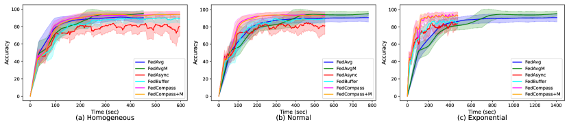
Figure 6: Change in validation accuracy during the training process for different FL algorithms on the class partitioned MNIST dataset with five clients and three client heterogeneity settings.

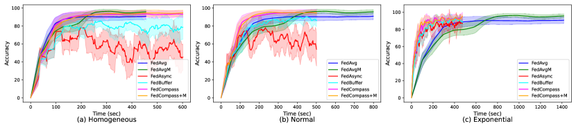
Figure 7: Change in validation accuracy during the training process for different FL algorithms on the class partitioned MNIST dataset with ten clients and three client heterogeneity settings.

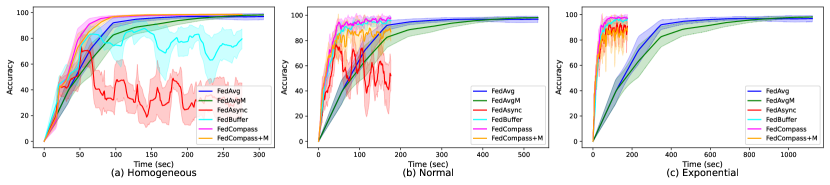
Figure 8: Change in validation accuracy during the training process for different FL algorithms on the class partitioned MNIST dataset with twenty clients and three client heterogeneity settings.

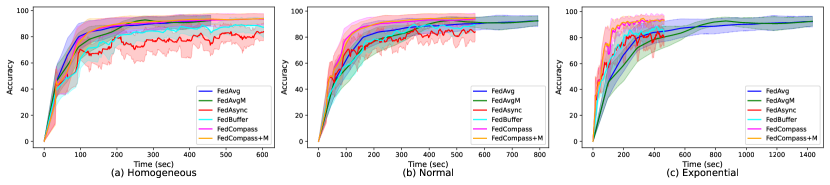
Figure 9: Change in validation accuracy during the training process for different FL algorithms on the dual Dirichlet partitioned MNIST dataset with five clients and three client heterogeneity settings.

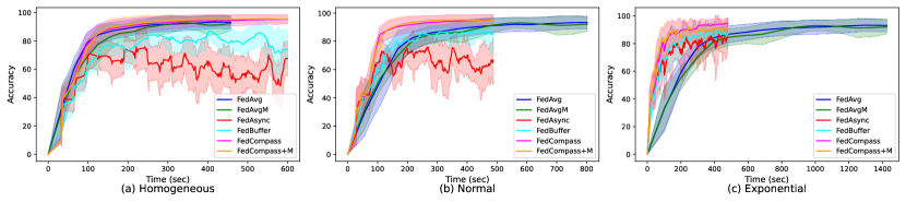
Figure 10: Change in validation accuracy during the training process for different FL algorithms on the dual Dirichlet partitioned MNIST dataset with ten clients and three client heterogeneity settings.

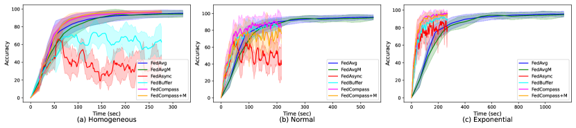
Figure 11: Change in validation accuracy during the training process for different FL algorithms on the dual Dirichlet partitioned MNIST dataset with twenty clients and three client heterogeneity settings.

F.2 Additional Experiment Results on the CIFAR-10 Dataset

Table 16 shows the top validation accuracy and the corresponding standard deviation on the class partitioned CIFAR-10 dataset for various federated learning algorithms with different numbers of clients and client heterogeneity settings among ten independent experiment runs with different random seeds, and Table 17 shows that on the dual Dirichlet partitioned CIFAR-10 dataset. Figures 12 to 17 give the change in validation accuracy during the training process for various FL algorithms in different experiment settings on the CIFAR-10 datasets.

Table 16: Average top accuracy and standard deviation on the class partitioned CIFAR-10 dataset for various FL algorithms with different numbers of clients and client heterogeneity settings.

		$m=5$				$m=10$				$m=20$
Method		homo	normal	exp		homo	normal	exp		homo	normal	exp
FedAvg		67.10$\pm$6.33	67.10$\pm$6.33	67.10$\pm$6.3		66.80$\pm$2.71	66.80$\pm$2.71	66.80$\pm$2.71		70.03$\pm$2.37	70.03$\pm$2.37	70.03$\pm$2.37
FedAvgM		63.44$\pm$3.26	63.44$\pm$3.26	63.44$\pm$3.26		63.50$\pm$2.56	63.50$\pm$2.56	63.50$\pm$2.56		64.47$\pm$1.88	64.47$\pm$1.88	64.47$\pm$1.88
FedAsync		53.30$\pm$4.12	63.65$\pm$2.81	66.27$\pm$3.91		37.09$\pm$2.99	44.87$\pm$3.54	59.40$\pm$4.21		30.18$\pm$2.84	36.73$\pm$4.93	54.30$\pm$2.64
FedBuffer		67.02$\pm$2.55	67.33$\pm$2.46	70.86$\pm$2.99		46.14$\pm$4.14	50.86$\pm$4.43	64.32$\pm$3.78		43.83$\pm$3.01	49.63$\pm$4.60	60.90$\pm$3.37
FedCompass		72.66$\pm$2.44	73.64$\pm$1.80	73.96$\pm$1.83		66.27$\pm$2.41	67.07$\pm$2.40	68.73$\pm$1.95		66.83$\pm$1.29	67.14$\pm$1.32	67.41$\pm$1.59
FedCompass+M		72.82$\pm$2.27	74.03$\pm$1.77	74.22$\pm$1.98		66.79$\pm$1.93	67.72$\pm$1.77	69.14$\pm$1.78		66.80$\pm$1.18	67.48$\pm$1.38	67.91$\pm$1.45

Table 17: Average top accuracy and standard deviation on the dual Dirichlet partitioned CIFAR-10 dataset for various FL algorithms with different numbers of clients and client heterogeneity settings.

		$m=5$				$m=10$				$m=20$
Method		homo	normal	exp		homo	normal	exp		homo	normal	exp
FedAvg		48.88$\pm$8.03	48.88$\pm$8.03	48.88$\pm$8.03		51.91$\pm$7.65	51.91$\pm$7.65	51.91$\pm$7.65		49.28$\pm$2.62	49.28$\pm$2.62	49.28$\pm$2.62
FedAvgM		49.89$\pm$5.27	49.89$\pm$5.27	49.89$\pm$5.27		51.72$\pm$2.64	51.72$\pm$2.64	51.72$\pm$2.64		49.94$\pm$4.15	49.94$\pm$4.15	49.94$\pm$4.15
FedAsync		44.38$\pm$4.71	47.67$\pm$4.29	51.21$\pm$4.99		33.52$\pm$3.29	38.13$\pm$2.07	47.62$\pm$2.59		34.89$\pm$3.34	36.12$\pm$1.69	39.92$\pm$3.39
FedBuffer		51.85$\pm$3.23	54.03$\pm$4.84	58.11$\pm$4.62		42.60$\pm$2.47	45.24$\pm$1.12	53.04$\pm$2.45		41.37$\pm$2.85	42.65$\pm$1.70	46.30$\pm$2.90
FedCompass		59.29$\pm$3.49	59.98$\pm$3.65	61.23$\pm$2.67		54.51$\pm$3.50	54.95$\pm$3.68	57.29$\pm$1.98		51.01$\pm$2.20	52.03$\pm$2.75	51.39$\pm$2.12
FedCompass+M		59.29$\pm$2.65	60.20$\pm$3.01	59.73$\pm$3.97		54.24$\pm$4.21	54.53$\pm$3.14	56.30$\pm$2.87		51.48$\pm$2.54	52.73$\pm$2.61	51.70$\pm$2.06

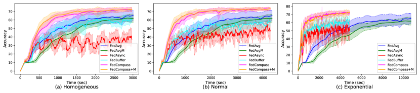
Figure 12: Change in validation accuracy during the training process for different FL algorithms on the class partitioned CIFAR-10 dataset with five clients and three client heterogeneity settings.

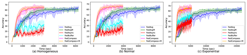
Figure 13: Change in validation accuracy during the training process for different FL algorithms on the class partitioned CIFAR-10 dataset with ten clients and three client heterogeneity settings.

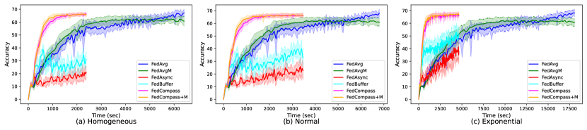
Figure 14: Change in validation accuracy during the training process for different FL algorithms on the class partitioned CIFAR-10 dataset with twenty clients and three client heterogeneity settings.

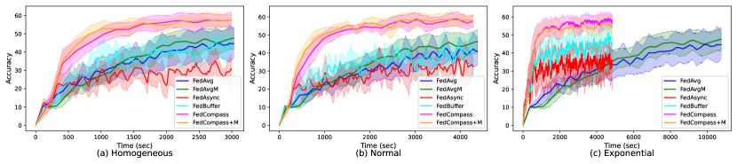
Figure 15: Change in validation accuracy during the training process for different FL algorithms on the dual Dirichlet partitioned CIFAR-10 dataset with five clients and three client heterogeneity settings.

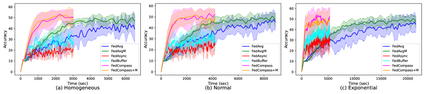
Figure 16: Change in validation accuracy during the training process for different FL algorithms on the dual Dirichlet partitioned CIFAR-10 dataset with ten clients and three client heterogeneity settings.

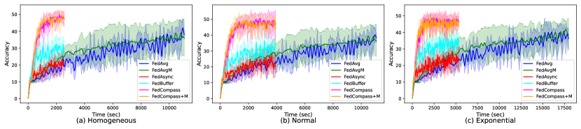
Figure 17: Change in validation accuracy during the training process for different FL algorithms on the dual Dirichlet partitioned CIFAR-10 dataset with twenty clients and three client heterogeneity settings.

F.3 Additional Experiment Results on the FLamby Datasets

Table 18 shows the top validation accuracy and the corresponding standard deviation on the Fed-IXI and Fed-ISIC2019 datasets from FLamby for various federated learning algorithms in different client heterogeneity settings among ten independent experiment runs with different random seeds. Figures 18 and 19 present the change in validation accuracy during the training process for various FL algorithms on the Fed-IXI and Fed-ISIC2019 datasets, respectively.

Table 18: Average top accuracy and standard deviation on the FLamby datasets for various federated learning methods in different client heterogeneity settings.

		Fed-IXI				Fed-ISIC2019
Method		homo	normal	exp		homo	normal	exp
FedAvg		98.39$\pm$0.02	98.39$\pm$0.02	98.39$\pm$0.02		59.12$\pm$1.38	59.12$\pm$1.38	59.12$\pm$1.38
FedAvgM		98.39$\pm$0.00	98.39$\pm$0.00	98.39$\pm$0.00		50.25$\pm$2.57	50.25$\pm$2.57	50.25$\pm$2.57
FedAsync		98.05$\pm$0.25	98.24$\pm$0.18	98.32$\pm$0.20		59.43$\pm$1.18	59.66$\pm$3.04	56.34$\pm$4.34
FedBuffer		98.36$\pm$0.03	98.35$\pm$0.03	98.35$\pm$0.08		57.65$\pm$2.07	57.46$\pm$2.60	55.13$\pm$4.74
FedCompass		98.76$\pm$0.00	98.61$\pm$0.06	98.59$\pm$0.04		68.46$\pm$0.38	66.35$\pm$3.76	65.46$\pm$5.33
FedCompass+M		98.76$\pm$0.00	98.61$\pm$0.06	98.59$\pm$0.04		64.72$\pm$0.94	62.43$\pm$5.23	60.18$\pm$4.95

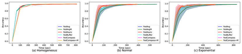
Figure 18: Change in validation accuracy during the training process for different federated learning algorithms on the FLamby Fed-IXI dataset with three different client heterogeneity settings.

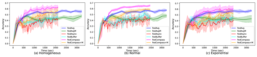
Figure 19: Change in validation accuracy during the training process for different federated learning algorithms on the FLamby Fed-ISIC2019 dataset with three different client heterogeneity settings.

Appendix G Ablation Study

G.1 Ablation Study on $Q_{\min}/Q_{\max}$

In this section, we conduct ablation studies on the values of $\textit{1/Q}=Q_{\min}/Q_{\max}$ to investigate its impact on the performance of the FedCompass algorithm. Table 19 lists the relative wall-clock time for different values of $\textit{1/Q}=Q_{\min}/Q_{\max}$ to reach 90% validation accuracy on the class partitioned and dual Dirichlet partitioned MNIST datasets in different client heterogeneity settings, and Table 20 shows the corresponding the validation accuracy and standard deviations. The results are the average of ten different runs with random seeds. Table 19 also lists the results of FedBuffer for reference. From Table 19, the following observations can be derived: (1) A smaller $Q_{\min}$ usually leads to faster convergence speed, which is consistent with the convergence analysis from Section 4 where smaller 1/Q results in fewer existing arrival groups at equilibrium and may help to reduce the impact of device heterogeneity. (2) Though FedCompass achieves faster convergence rate with smaller 1/Q (0.05 - 0.2) in general, it still can achieve reasonable convergence rate with large 1/Q values (0.2 - 0.8) compared with FedBuffer, which shows that FedCompass is not sensitive to the choice of the value of Q. (3) In the extreme case that $\textit{Q}=1$, i.e. $Q_{\min}=Q_{\max}$, there is a significant performance drop for FedCompass, as the Compass scheduler is not able to assign different number of local steps to different clients, so each client has its own group and the FedCompass algorithm becomes equivalent to the FedAsync algorithm.

Table 19: Relative wall-clock time to first reach the target validation accuracy on the MNIST datasets for various values of $\textit{1/Q}=Q_{\min}/Q_{\max}$ with different number of clients and client heterogeneity settings.

			$m=5$				$m=10$				$m=20$
Dataset	1/Q		homo	normal	exp		homo	normal	exp		homo	normal	exp
	0.05		1.04$\times$	1.16$\times$	0.92$\times$		0.93$\times$	0.90$\times$	0.95$\times$		0.98$\times$	0.93$\times$	0.99$\times$
	0.10		1.00$\times$	1.38$\times$	0.93$\times$		1.03$\times$	0.92$\times$	0.93$\times$		1.01$\times$	1.03$\times$	1.02$\times$
	0.20		1.00$\times$	1.00$\times$	1.00$\times$		1.00$\times$	1.00$\times$	1.00$\times$		1.00$\times$	1.00$\times$	1.00$\times$
MNIST-Class	0.40		0.99$\times$	1.67$\times$	2.48$\times$		0.98$\times$	0.98$\times$	1.41$\times$		1.01$\times$	1.19$\times$	1.10$\times$
Partition (90%)	0.60		0.97$\times$	1.23$\times$	2.64$\times$		0.98$\times$	0.97$\times$	1.28$\times$		1.02$\times$	1.31$\times$	1.11$\times$
	0.80		0.96$\times$	1.33$\times$	1.51$\times$		0.98$\times$	1.21$\times$	1.23$\times$		1.01$\times$	1.61$\times$	1.28$\times$
	1.00		2.15$\times$	2.34$\times$	2.35$\times$		-	2.17$\times$	1.32$\times$		-	4.44$\times$	1.32$\times$
FedBuffer			1.30$\times$	1.57$\times$	1.81$\times$		1.58$\times$	1.39$\times$	1.43$\times$		1.37$\times$	1.18$\times$	1.39$\times$
	0.05		0.89$\times$	1.01$\times$	0.85$\times$		0.96$\times$	0.97$\times$	0.82$\times$		1.00$\times$	1.02$\times$	0.96$\times$
	0.10		0.91$\times$	1.05$\times$	0.92$\times$		0.96$\times$	0.95$\times$	0.85$\times$		0.97$\times$	1.02$\times$	0.96$\times$
	0.20		1.00$\times$	1.00$\times$	1.00$\times$		1.00$\times$	1.00$\times$	1.00$\times$		1.00$\times$	1.00$\times$	1.00$\times$
MNIST-Dirichlet	0.40		1.02$\times$	1.03$\times$	1.70$\times$		1.04$\times$	1.05$\times$	1.28$\times$		1.00$\times$	1.14$\times$	1.25$\times$
Partition (90%)	0.60		1.04$\times$	1.01$\times$	1.83$\times$		1.00$\times$	1.01$\times$	1.19$\times$		0.92$\times$	1.11$\times$	1.16$\times$
	0.80		1.04$\times$	1.13$\times$	1.58$\times$		0.91$\times$	1.25$\times$	1.22$\times$		0.86$\times$	1.22$\times$	1.21$\times$
	1.00		1.78$\times$	1.68$\times$	2.01$\times$		-	2.28$\times$	1.29$\times$		-	-	1.76$\times$
FedBuffer			1.23$\times$	1.52$\times$	1.86$\times$		1.81$\times$	1.51$\times$	1.49$\times$		2.77$\times$	1.22$\times$	1.40$\times$

Table 20: Average top validation accuracy and standard deviation for various values of $\textit{1/Q}=Q_{\min}/Q_{\max}$ with different number of clients and client heterogeneity settings.

			$m=5$				$m=10$				$m=20$
Dataset	1/Q		homo	normal	exp		homo	normal	exp		homo	normal	exp
	0.05		95.20$\pm$2.53	95.21$\pm$2.90	97.22$\pm$1.67		94.29$\pm$3.80	94.88$\pm$3.73	97.49$\pm$1.55		98.56$\pm$0.43	98.80$\pm$0.17	98.75$\pm$0.20
	0.10		95.03$\pm$3.13	95.35$\pm$2.15	97.07$\pm$1.67		94.72$\pm$3.56	94.65$\pm$3.74	97.71$\pm$1.25		98.57$\pm$0.38	98.80$\pm$0.11	98.82$\pm$0.18
MNIST	0.20		95.06$\pm$2.89	95.55$\pm$2.89	96.34$\pm$1.89		94.33$\pm$3.80	95.47$\pm$3.05	97.51$\pm$1.66		98.49$\pm$0.45	98.67$\pm$0.36	98.73$\pm$0.47
Class	0.40		94.44$\pm$3.26	95.34$\pm$3.63	92.73$\pm$3.09		94.42$\pm$3.94	95.01$\pm$3.52	96.91$\pm$2.13		98.58$\pm$0.36	98.74$\pm$0.26	98.75$\pm$0.32
Partition	0.60		95.29$\pm$2.75	95.25$\pm$3.36	94.90$\pm$0.97		94.17$\pm$3.88	95.38$\pm$2.55	97.73$\pm$0.86		98.48$\pm$0.56	98.80$\pm$0.20	98.80$\pm$0.19
(90%)	0.80		95.61$\pm$2.34	95.35$\pm$2.30	95.04$\pm$3.13		94.77$\pm$3.59	96.08$\pm$2.60	97.35$\pm$1.49		98.60$\pm$0.45	98.72$\pm$0.25	98.74$\pm$0.25
	1.00		90.60$\pm$6.96	92.53$\pm$5.57	92.44$\pm$3.07		86.73$\pm$6.62	92.27$\pm$3.82	96.25$\pm$2.46		84.26$\pm$7.96	90.98$\pm$2.48	98.01$\pm$0.89
	0.05		94.10$\pm$4.12	94.30$\pm$4.18	95.81$\pm$3.12		95.64$\pm$3.15	95.75$\pm$2.98	96.17$\pm$3.01		96.22$\pm$2.25	97.40$\pm$1.82	97.04$\pm$1.97
	0.10		94.14$\pm$4.08	94.14$\pm$4.44	96.11$\pm$3.04		95.49$\pm$3.32	95.65$\pm$3.23	96.78$\pm$2.56		96.39$\pm$1.92	97.59$\pm$1.28	97.68$\pm$1.28
MNIST	0.20		94.15$\pm$4.26	94.36$\pm$4.28	95.46$\pm$3.59		95.53$\pm$3.21	95.41$\pm$3.52	96.34$\pm$2.64		96.41$\pm$1.96	97.62$\pm$1.57	97.86$\pm$0.71
Dirichlet	0.40		94.12$\pm$4.11	94.27$\pm$4.11	95.40$\pm$2.46		95.46$\pm$3.47	95.67$\pm$3.14	95.86$\pm$3.35		96.07$\pm$2.45	98.03$\pm$0.93	97.85$\pm$1.00
Partition	0.60		94.09$\pm$4.10	94.65$\pm$4.11	94.29$\pm$3.43		95.43$\pm$3.36	95.89$\pm$3.26	95.27$\pm$4.71		96.37$\pm$2.35	98.04$\pm$0.68	97.66$\pm$1.14
(90%)	0.80		94.23$\pm$3.89	94.71$\pm$3.56	95.09$\pm$2.62		95.32$\pm$3.55	95.46$\pm$3.20	95.26$\pm$4.36		96.72$\pm$2.20	97.51$\pm$0.84	97.66$\pm$0.62
	1.00		92.11$\pm$2.99	92.96$\pm$3.70	93.29$\pm$3.08		86.31$\pm$4.51	90.72$\pm$4.30	94.06$\pm$5.91		78.49$\pm$6.28	85.82$\pm$5.31	95.90$\pm$1.58

G.2 Client Speed Changes in FedCompass and Ablation Study on $\lambda$

In cross-silo federated learning scenarios, variations in computing power and speeds among clients are frequent occurrences. For instance, a client utilizing a supercomputer might experience fluctuations in computing power due to the allocation or deallocation of additional tasks within the same cluster. In this section, we provide analyses and empirical results to study how FedCompass is resilient to client speed changes.

Figure 20 depicts an execution of FedCompass involving a client speedup scenario. During the second round of local training, client 3 enhances its computing speed from $4$ step/min to $5$ step/min. Consequently, client 3 transmits its local updates $\Delta_{3}$ at 10:36, earlier than the expected group arrival time $T_{a}=$ 12:00. In this situation, FedCompass server first updates the speed record for client 3 and then waits for the arrival of clients 1 and 2 in the same group. Upon the arrival of clients 1 and 2 at 12:00, FedCompass server assigns all three clients to arrival group 2 for the subsequent round of local training, and the number of local steps for client 3 are assigned according to its new speed.

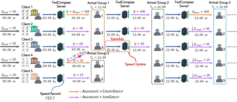
Figure 20: Overview of an execution of FedCompass on five clients with the minimum number of local steps $Q_{\min}=20$, maximum number of local steps $Q_{\max}=100$, and client speedup.

Figures 21 and 22 illustrate two executions of FedCompass with different levels of client slowdown. In Figure 21, the speed of client 3 changes from $4$ step/min to $3.33$ step/min during its second round of training. Consequently, the client transmits its local update $\Delta_{3}$ back to the server at 13:24, surpassing the expected arrival time $T_{a}=$ 12:00. Nonetheless, it is important to recall that each arrival group has the latest arrival time $T_{\max}$ to accommodate potential client speed fluctuations. The time interval between $T_{\max}$ and the group’s creation time is $\lambda$ times longer than the difference between $T_{a}$ and the group’s creation time. For this example, we select $\lambda=1.2$, resulting in $T_{\max}=$ 14:00 for arrival group 1. Since client 3 arrives later than $T_{a}$ but earlier than $T_{\max}$, FedCompass server waits until client 3 arrives at 13:24, subsequently assigning clients 1 to 3 to a new arrival group for the next training round. Figure 22 presents another case where the client has a relatively larger slowdown. In this example, the speed of client 3 diminishes from $4$ step/min to $2.5$ step/min, causing it to transmit local update $\Delta_{3}$ at 15:12, even exceeding $T_{\max}=$ 14:00. When FedCompass server does not receive an update from client 3 by the latest arrival time 14:00, it responds to clients 1 and 2. The server assigns these clients to arrival group 2 with corresponding numbers of local steps. Upon client 3 arrives at 15:12, the server first attempts to assign it to group 2, but this is unsuccessful due to the corresponding number of steps ($Q=\text{(22:00-15:12)}*2.5\text{ (step/min)}=17$) falling below the $Q_{\min}=20$. As a result, the server establishes a new group 3 for client 3. Subsequently, once all clients in group 2 arrive at $22:00$, the server assigns all of them to group 3.

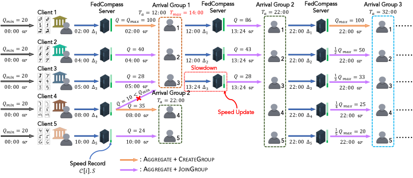
Figure 21: Overview of an execution of FedCompass on five clients with the minimum number of local steps $Q_{\min}=20$ and maximum number of local steps $Q_{\max}=100$ with client slowdown.

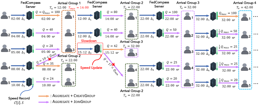
Figure 22: Overview of an execution of FedCompass on five clients with the minimum number of local steps $Q_{\min}=20$ and maximum number of local steps $Q_{\max}=100$ with client slowdown.

To empirically study how FedCompass is resilient to client speed changes and how the value of $\lambda$ may impact the resilience, we set up a scenario such that each client has a 10% probability to change its computing speed by re-sampling a speed from the client speed distribution in each local training round. Table 21 shows the convergence speed for the FedCompass algorithm with different values of $\lambda$, and Table 22 shows the corresponding average top accuracy and standard deviations. From Table 21, we can draw the following conclusions: (1) When $\lambda=1.00$, the Compass scheduler is not resilient to even small client slowdown, so FedCompass converges relatively slower compared with some $\lambda$ values slightly above $1.00$ in general. (2) $\lambda$ values slightly above $1.00$ (e.g., $1.20-1.50$) result in faster convergence from the empirical results as the Compass scheduler accounts for minor client speed fluctuations without a long waiting time. (3) Large $\lambda$ values sometimes slow down the convergence as the server needs to experience a long waiting time when there are significant client speed slowdowns.

Table 21: Relative wall-clock time to first reach the target validation accuracy on the MNIST datasets for various values of $\lambda$ with different number of clients and client heterogeneity settings, and each client has 10% probability to change its speed in each local training round.

			$m=5$			$m=10$			$m=20$
Dataset	$\lambda$		normal	exp		normal	exp		normal	exp
	1.00		1.00$\times$	1.00$\times$		1.00$\times$	1.00$\times$		1.00$\times$	1.00$\times$
MNIST-Class	1.20		0.64$\times$	0.83$\times$		0.84$\times$	0.88$\times$		0.86$\times$	0.90$\times$
Partition (90%)	1.50		0.67$\times$	1.00$\times$		0.72$\times$	1.01$\times$		1.01$\times$	1.00$\times$
	2.00		0.68$\times$	1.11$\times$		0.80$\times$	1.11$\times$		1.04$\times$	1.37$\times$
	1.00		1.00$\times$	1.00$\times$		1.00$\times$	1.00$\times$		1.00$\times$	1.00$\times$
MNIST-Dirichlet	1.20		0.63$\times$	1.05$\times$		0.75$\times$	0.62$\times$		0.79$\times$	0.98$\times$
Partition (90%)	1.50		0.55$\times$	1.20$\times$		0.75$\times$	0.62$\times$		0.85$\times$	1.16$\times$
	2.00		0.55$\times$	1.29$\times$		0.76$\times$	0.83$\times$		0.86$\times$	1.28$\times$

Table 22: Average top validation accuracy and standard deviation on the MNIST datasets for various values of $\lambda$ with different number of clients and client heterogeneity settings, and each client has 10% probability to change its speed in each local training round.

			$m=5$			$m=10$			$m=20$
Dataset	$\lambda$		normal	exp		normal	exp		normal	exp
	1.00		97.01$\pm$1.19	97.57$\pm$1.01		96.55$\pm$1.07	97.45$\pm$2.17		98.78$\pm$0.03	98.76$\pm$0.15
MNIST-Class	1.20		96.19$\pm$2.46	97.54$\pm$1.54		96.78$\pm$2.94	97.03$\pm$2.71		98.86$\pm$0.10	98.90$\pm$0.05
Partition (90%)	1.50		95.99$\pm$2.30	97.59$\pm$1.98		96.25$\pm$3.26	97.44$\pm$1.90		98.86$\pm$0.09	98.71$\pm$0.26
	2.00		96.29$\pm$1.77	97.84$\pm$1.06		96.37$\pm$3.17	97.37$\pm$2.29		98.86$\pm$0.09	98.83$\pm$0.13
	1.00		91.15$\pm$4.48	94.34$\pm$2.84		94.88$\pm$4.40	96.90$\pm$1.53		98.08$\pm$0.34	98.09$\pm$0.23
MNIST-Dirichlet	1.20		92.03$\pm$4.10	93.92$\pm$3.45		96.59$\pm$2.10	97.19$\pm$1.82		98.16$\pm$0.13	98.22$\pm$0.19
Partition (90%)	1.50		91.82$\pm$4.35	93.32$\pm$4.03		96.04$\pm$3.36	97.47$\pm$1.42		98.28$\pm$0.13	98.16$\pm$0.19
	2.00		92.09$\pm$4.11	93.08$\pm$3.61		95.77$\pm$3.29	97.36$\pm$1.68		98.16$\pm$0.20	98.26$\pm$0.07

References

- Bonawitz et al. (2019) Keith Bonawitz, Hubert Eichner, Wolfgang Grieskamp, Dzmitry Huba, Alex Ingerman, Vladimir Ivanov, Chloe Kiddon, Jakub Konečnỳ, Stefano Mazzocchi, Brendan McMahan, et al. Towards federated learning at scale: System design. Proceedings of machine learning and systems, 1:374–388, 2019.
- Chai et al. (2021) Zheng Chai, Yujing Chen, Ali Anwar, Liang Zhao, Yue Cheng, and Huzefa Rangwala. Fedat: A high-performance and communication-efficient federated learning system with asynchronous tiers. In Proceedings of the International Conference for High Performance Computing, Networking, Storage and Analysis, pp. 1–16, 2021.
- Chen et al. (2019) Yang Chen, Xiaoyan Sun, and Yaochu Jin. Communication-efficient federated deep learning with layerwise asynchronous model update and temporally weighted aggregation. IEEE transactions on neural networks and learning systems, 31(10):4229–4238, 2019.
- Chen et al. (2020) Yujing Chen, Yue Ning, Martin Slawski, and Huzefa Rangwala. Asynchronous online federated learning for edge devices with non-iid data. In 2020 IEEE International Conference on Big Data (Big Data), pp. 15–24. IEEE, 2020.
- Chen et al. (2021) Zheyi Chen, Weixian Liao, Kun Hua, Chao Lu, and Wei Yu. Towards asynchronous federated learning for heterogeneous edge-powered internet of things. Digital Communications and Networks, 7(3):317–326, 2021.
- Çiçek et al. (2016) Özgün Çiçek, Ahmed Abdulkadir, Soeren S Lienkamp, Thomas Brox, and Olaf Ronneberger. 3d u-net: learning dense volumetric segmentation from sparse annotation. In Medical Image Computing and Computer-Assisted Intervention–MICCAI 2016: 19th International Conference, Athens, Greece, October 17-21, 2016, Proceedings, Part II 19, pp. 424–432. Springer, 2016.
- Codella et al. (2018) Noel CF Codella, David Gutman, M Emre Celebi, Brian Helba, Michael A Marchetti, Stephen W Dusza, Aadi Kalloo, Konstantinos Liopyris, Nabin Mishra, Harald Kittler, et al. Skin lesion analysis toward melanoma detection: A challenge at the 2017 international symposium on biomedical imaging (isbi), hosted by the international skin imaging collaboration (isic). In 2018 IEEE 15th international symposium on biomedical imaging (ISBI 2018), pp. 168–172. IEEE, 2018.
- Combalia et al. (2019) Marc Combalia, Noel CF Codella, Veronica Rotemberg, Brian Helba, Veronica Vilaplana, Ofer Reiter, Cristina Carrera, Alicia Barreiro, Allan C Halpern, Susana Puig, et al. Bcn20000: Dermoscopic lesions in the wild. arXiv preprint arXiv:1908.02288, 2019.
- Deng et al. (2009) Jia Deng, Wei Dong, Richard Socher, Li-Jia Li, Kai Li, and Li Fei-Fei. Imagenet: A large-scale hierarchical image database. In 2009 IEEE conference on computer vision and pattern recognition, pp. 248–255. Ieee, 2009.
- Dice (1945) Lee R Dice. Measures of the amount of ecologic association between species. Ecology, 26(3):297–302, 1945.
- Hao et al. (2020) Jiangshan Hao, Yanchao Zhao, and Jiale Zhang. Time efficient federated learning with semi-asynchronous communication. In 2020 IEEE 26th International Conference on Parallel and Distributed Systems (ICPADS), pp. 156–163. IEEE, 2020.
- He et al. (2016) Kaiming He, Xiangyu Zhang, Shaoqing Ren, and Jian Sun. Deep residual learning for image recognition. In Proceedings of the IEEE conference on computer vision and pattern recognition, pp. 770–778, 2016.
- Hsu et al. (2019) Tzu-Ming Harry Hsu, Hang Qi, and Matthew Brown. Measuring the effects of non-identical data distribution for federated visual classification. arXiv preprint arXiv:1909.06335, 2019.
- Imteaj & Amini (2020) Ahmed Imteaj and M Hadi Amini. Fedar: Activity and resource-aware federated learning model for distributed mobile robots. In 2020 19th IEEE International Conference on Machine Learning and Applications (ICMLA), pp. 1153–1160. IEEE, 2020.
- Kairouz et al. (2021) Peter Kairouz, H Brendan McMahan, Brendan Avent, Aurélien Bellet, Mehdi Bennis, Arjun Nitin Bhagoji, Kallista Bonawitz, Zachary Charles, Graham Cormode, Rachel Cummings, et al. Advances and open problems in federated learning. Foundations and Trends® in Machine Learning, 14(1–2):1–210, 2021.
- Kaissis et al. (2021) Georgios Kaissis, Alexander Ziller, Jonathan Passerat-Palmbach, Théo Ryffel, Dmitrii Usynin, Andrew Trask, Ionésio Lima Jr, Jason Mancuso, Friederike Jungmann, Marc-Matthias Steinborn, et al. End-to-end privacy preserving deep learning on multi-institutional medical imaging. Nature Machine Intelligence, 3(6):473–484, 2021.
- Karimireddy et al. (2020) Sai Praneeth Karimireddy, Satyen Kale, Mehryar Mohri, Sashank Reddi, Sebastian Stich, and Ananda Theertha Suresh. Scaffold: Stochastic controlled averaging for federated learning. In International Conference on Machine Learning, pp. 5132–5143. PMLR, 2020.
- Konečnỳ et al. (2016) Jakub Konečnỳ, H Brendan McMahan, Felix X Yu, Peter Richtárik, Ananda Theertha Suresh, and Dave Bacon. Federated learning: Strategies for improving communication efficiency. arXiv preprint arXiv:1610.05492, 2016.
- Krizhevsky et al. (2009) Alex Krizhevsky, Geoffrey Hinton, et al. Learning multiple layers of features from tiny images. 2009.
- LeCun (1998) Yann LeCun. The mnist database of handwritten digits. http://yann. lecun. com/exdb/mnist/, 1998.
- Li et al. (2020) Tian Li, Anit Kumar Sahu, Ameet Talwalkar, and Virginia Smith. Federated learning: Challenges, methods, and future directions. IEEE signal processing magazine, 37(3):50–60, 2020.
- Li et al. (2019) Xiang Li, Kaixuan Huang, Wenhao Yang, Shusen Wang, and Zhihua Zhang. On the convergence of fedavg on non-iid data. arXiv preprint arXiv:1907.02189, 2019.
- Li et al. (2023) Zilinghan Li, Shilan He, Pranshu Chaturvedi, Trung-Hieu Hoang, Minseok Ryu, EA Huerta, Volodymyr Kindratenko, Jordan Fuhrman, Maryellen Giger, Ryan Chard, et al. Appflx: Providing privacy-preserving cross-silo federated learning as a service. arXiv preprint arXiv:2308.08786, 2023.
- Loshchilov & Hutter (2017) Ilya Loshchilov and Frank Hutter. Decoupled weight decay regularization. arXiv preprint arXiv:1711.05101, 2017.
- McMahan et al. (2017) Brendan McMahan, Eider Moore, Daniel Ramage, Seth Hampson, and Blaise Aguera y Arcas. Communication-efficient learning of deep networks from decentralized data. In Artificial intelligence and statistics, pp. 1273–1282. PMLR, 2017.
- Mills et al. (2019) Jed Mills, Jia Hu, and Geyong Min. Communication-efficient federated learning for wireless edge intelligence in iot. IEEE Internet of Things Journal, 7(7):5986–5994, 2019.
- Nguyen et al. (2022) John Nguyen, Kshitiz Malik, Hongyuan Zhan, Ashkan Yousefpour, Mike Rabbat, Mani Malek, and Dzmitry Huba. Federated learning with buffered asynchronous aggregation. In International Conference on Artificial Intelligence and Statistics, pp. 3581–3607. PMLR, 2022.
- Nishio & Yonetani (2019) Takayuki Nishio and Ryo Yonetani. Client selection for federated learning with heterogeneous resources in mobile edge. In ICC 2019-2019 IEEE international conference on communications (ICC), pp. 1–7. IEEE, 2019.
- Ogier du Terrail et al. (2022) Jean Ogier du Terrail, Samy-Safwan Ayed, Edwige Cyffers, Felix Grimberg, Chaoyang He, Regis Loeb, Paul Mangold, Tanguy Marchand, Othmane Marfoq, Erum Mushtaq, et al. Flamby: Datasets and benchmarks for cross-silo federated learning in realistic healthcare settings. Advances in Neural Information Processing Systems, 35:5315–5334, 2022.
- Pati et al. (2022) Sarthak Pati, Ujjwal Baid, Brandon Edwards, Micah Sheller, Shih-Han Wang, G Anthony Reina, Patrick Foley, Alexey Gruzdev, Deepthi Karkada, Christos Davatzikos, et al. Federated learning enables big data for rare cancer boundary detection. Nature communications, 13(1):7346, 2022.
- Pérez-García et al. (2021) Fernando Pérez-García, Rachel Sparks, and Sébastien Ourselin. Torchio: a python library for efficient loading, preprocessing, augmentation and patch-based sampling of medical images in deep learning. Computer Methods and Programs in Biomedicine, 208:106236, 2021.
- Reddi et al. (2020) Sashank Reddi, Zachary Charles, Manzil Zaheer, Zachary Garrett, Keith Rush, Jakub Konečnỳ, Sanjiv Kumar, and H Brendan McMahan. Adaptive federated optimization. arXiv preprint arXiv:2003.00295, 2020.
- Ryu et al. (2022) Minseok Ryu, Youngdae Kim, Kibaek Kim, and Ravi K Madduri. Appfl: open-source software framework for privacy-preserving federated learning. In 2022 IEEE International Parallel and Distributed Processing Symposium Workshops (IPDPSW), pp. 1074–1083. IEEE, 2022.
- Stich (2018) Sebastian U Stich. Local sgd converges fast and communicates little. arXiv preprint arXiv:1805.09767, 2018.
- Tan & Le (2019) Mingxing Tan and Quoc Le. Efficientnet: Rethinking model scaling for convolutional neural networks. In International conference on machine learning, pp. 6105–6114. PMLR, 2019.
- Tschandl et al. (2018) Philipp Tschandl, Cliff Rosendahl, and Harald Kittler. The ham10000 dataset, a large collection of multi-source dermatoscopic images of common pigmented skin lesions. Scientific data, 5(1):1–9, 2018.
- Wang (2019) Guan Wang. Interpret federated learning with shapley values. arXiv preprint arXiv:1905.04519, 2019.
- Wang et al. (2019) Guan Wang, Charlie Xiaoqian Dang, and Ziye Zhou. Measure contribution of participants in federated learning. In 2019 IEEE international conference on big data (Big Data), pp. 2597–2604. IEEE, 2019.
- Wang et al. (2020) Jianyu Wang, Qinghua Liu, Hao Liang, Gauri Joshi, and H Vincent Poor. Tackling the objective inconsistency problem in heterogeneous federated optimization. Advances in neural information processing systems, 33:7611–7623, 2020.
- Wang et al. (2021) Qizhao Wang, Qing Li, Kai Wang, Hong Wang, and Peng Zeng. Efficient federated learning for fault diagnosis in industrial cloud-edge computing. Computing, 103(10):2319–2337, 2021.
- Wu et al. (2020) Wentai Wu, Ligang He, Weiwei Lin, Rui Mao, Carsten Maple, and Stephen Jarvis. Safa: A semi-asynchronous protocol for fast federated learning with low overhead. IEEE Transactions on Computers, 70(5):655–668, 2020.
- Xie et al. (2019) Cong Xie, Sanmi Koyejo, and Indranil Gupta. Asynchronous federated optimization. arXiv preprint arXiv:1903.03934, 2019.
- Xu et al. (2021) Chenhao Xu, Youyang Qu, Yong Xiang, and Longxiang Gao. Asynchronous federated learning on heterogeneous devices: A survey. arXiv preprint arXiv:2109.04269, 2021.
- Yang et al. (2019) Qiang Yang, Yang Liu, Tianjian Chen, and Yongxin Tong. Federated machine learning: Concept and applications. ACM Transactions on Intelligent Systems and Technology (TIST), 10(2):1–19, 2019.
- Yu et al. (2019) Hao Yu, Sen Yang, and Shenghuo Zhu. Parallel restarted sgd with faster convergence and less communication: Demystifying why model averaging works for deep learning. In Proceedings of the AAAI Conference on Artificial Intelligence, volume 33, pp. 5693–5700, 2019.
- Yurochkin et al. (2019) Mikhail Yurochkin, Mayank Agarwal, Soumya Ghosh, Kristjan Greenewald, Nghia Hoang, and Yasaman Khazaeni. Bayesian nonparametric federated learning of neural networks. In International conference on machine learning, pp. 7252–7261. PMLR, 2019.
- Zhang et al. (2021) Yu Zhang, Morning Duan, Duo Liu, Li Li, Ao Ren, Xianzhang Chen, Yujuan Tan, and Chengliang Wang. Csafl: A clustered semi-asynchronous federated learning framework. In 2021 International Joint Conference on Neural Networks (IJCNN), pp. 1–10. IEEE, 2021.