Model averaging: A shrinkage perspective

Abstract

Model averaging (MA), a technique for combining estimators from a set of candidate models, has attracted increasing attention in machine learning and statistics. In the existing literature, there is an implicit understanding that MA can be viewed as a form of shrinkage estimation that draws the response vector towards the subspaces spanned by the candidate models. This paper explores this perspective by establishing connections between MA and shrinkage in a linear regression setting with multiple nested models. We first demonstrate that the optimal MA estimator is the best linear estimator with monotone non-increasing weights in a Gaussian sequence model. The Mallows MA, which estimates weights by minimizing the Mallows’ $C_{p}$, is a variation of the positive-part Stein estimator. Motivated by these connections, we develop a novel MA procedure based on a blockwise Stein estimation. Our resulting Stein-type MA estimator is asymptotically optimal across a broad parameter space when the variance is known. Numerical results support our theoretical findings. The connections established in this paper may open up new avenues for investigating MA from different perspectives. A discussion on some topics for future research concludes the paper.

Keywords: Model averaging, Stein shrinkage, penalized blockwise Stein rule, asymptotic optimality.

1 Introduction

Model averaging (MA) is an umbrella term for methods that combine multiple candidate models to make a decision, typically in regression and forecasting problems. The concept of MA was first introduced by de Laplace, (1818) (see Moral-Benito,, 2015, for a comprehensive review of the historical development of MA). In recent years, MA has received an explosion of interest in both machine learning and statistics (see, e.g., Fletcher,, 2018). It is regarded as a viable alternative to model selection (MS) techniques, as it aims to mitigate MS variability and control modeling biases among candidate models. The benefits of MA compared to MS have been theoretically studied in Peng and Yang, (2022).

In the existing literature, MA has been approached using either Bayesian or frequentist frameworks. The Bayesian perspective on MA can be found in works such as Draper, (1995), George and Mcculloch, (1997), and Hoeting et al., (1999). Within the frequentist paradigm, MA strategies have become increasingly popular in forecasting literature since the works of Barnard, (1963) and Bates and Granger, (1969) (see Timmermann,, 2006, for a review on the literature). In recent years, several important techniques has been developed, including boosting (Freund,, 1995), bagging (Breiman, 1996a, ), stacking (Wolpert,, 1992; Breiman, 1996b, ), random forest (Amit and Geman,, 1997), information criterion weighting (Buckland et al.,, 1997; Hjort and Claeskens,, 2003), adaptive regression by mixing (Yang,, 2001; Yuan and Yang,, 2005), exponential weighting (George,, 1986; Leung and Barron,, 2006; Dalalyan and Salmon,, 2012), and Q-aggregation (Rigollet,, 2012; Dai et al.,, 2014; Bellec,, 2018). Additionally, there is a growing body of literature focused on constructing asymptotically optimal MA, with the goal of finding the optimal convex combination of candidate estimates. This is typically achieved by minimizing performance measures such as Mallows’ $C_{p}$ (see, e.g., Blaker,, 1999; Hansen,, 2007; Wan et al.,, 2010) or cross-validation error (see, e.g., Hansen and Racine,, 2012; Zhang et al.,, 2013; Ando and Li,, 2014).

Despite the extensive theoretical work and wide applications of MA, there is a commonly held viewpoint that MA is essentially a shrinkage estimator, and that other shrinkage methods can also achieve the objectives of MA. This view has been substantiated by several studies. For instance, the results in Section 5.1 of Kneip, (1994) indicate that combining two linear smoothers by minimizing Mallows’ $C_{p}$ yields a James-Stein estimator. The relationship between Mallows model averaging (MMA) and Stein shrinkage estimation has been further explored in Blaker, (1999), Hansen, (2007), and Hansen, (2014) in the context of two nested models. In a semiparametric regression setting, Ullah et al., (2017) established the connection between MA and ridge shrinkage on the basis of the orthogonal model. Additionally, in a Gaussian location model, Green and Strawderman, (1991) proposed a James-Stein type estimator to estimate the best linear combination of two independent biased and unbiased estimators. The independence assumption between two estimators in Green and Strawderman, (1991) has been relaxed by Kim and White, (2001), Judge and Mittelhammer, (2004), and Mittelhammer and Judge, (2005). More recently, Hansen, (2016) proposed a Stein method to combine the restricted and unrestricted maximum likelihood estimators in a local asymptotic framework, and showed the asymptotic risk of this shrinkage estimator is strictly less than that of the maximum likelihood estimator.

Note that most of the aforementioned studies focused on the relationship between MA and shrinkage in a two-model setting. The fundamental question that remains to be explored is whether these links persist in the context of multiple models. If so, can some state-of-the-art shrinkage techniques be employed to create MA estimators that perform as optimally as the infeasible optimal convex combinations of candidate models (i.e., the asymptotically optimal MA estimators)? Such answers would have a significant impact on the theories and applications of MA.

This paper addresses the previously mentioned questions in a general linear model setting with multiple nested candidate models. The main contribution is twofold. First, we demonstrate that the optimal MA estimator is equivalent to the optimal linear estimator with monotonically non-increasing weights in a specific Gaussian sequence model. And the MMA estimator (Hansen,, 2007), which targets the optimal MA risk, can be regarded as a variation of the sum of a set of positive-part Stein estimators from multiple mutually orthogonal subspaces. Second, we introduce a novel MA procedure to achieve asymptotic optimality by adapting the blockwise Stein rules from prior works (Donoho and Johnstone,, 1995; Nemirovski,, 1998; Cavalier and Tsybakov,, 2001) to linear regression. In particular, when the candidate model set is properly constructed, this Stein-type MA estimator achieves the full potential of MA (i.e., the minimal MA risk over all the nested models) in a sufficiently large parameter space. The results of finite sample simulations support our theories.

This paper gives the opportunity of looking at MA from different angles. By connecting MA with shrinkage, existing knowledge and technology derived from shrinkage estimation can be potentially transferred to MA. The selected review presented in this paper and the unveiled connections provide a theoretical foundation for this transfer; See Section 6 for more discussion.

The remainder of the paper is structured as follows. In Section 2, we set up our regression problem. Section 3 draws the theoretical connections between MA and shrinkage. In Section 4, we propose a Stein-type MA procedure and present its theoretical properties. Section 5 examines the finite sample properties of proposed methods by numerical simulations, and Section 6 concludes the paper. Proofs are included in the Appendix.

2 Problem setup

Consider the linear regression model

$$y_{i}=\mu_{i}+\varepsilon_{i}=\sum_{j=1}^{p_{n}}\beta_{j}x_{ij}+\varepsilon_{i},\quad i=1,\ldots,n,$$ (2.1)

where $\varepsilon_{1},\ldots,\varepsilon_{n}$ are independent normal errors with mean $0$ and variance $\sigma^{2}$, $x_{i1},\ldots,x_{ip_{n}}$ are non-stochastic variables, and $p_{n}$ is the number of regressors. Let $\mathbf{y}=(y_{1},\ldots,y_{n})^{\top}$, $\bm{\mu}=(\mu_{1},\ldots,\mu_{n})^{\top}$, $\bm{\varepsilon}=(\varepsilon_{1},\ldots,\varepsilon_{n})^{\top}$, $\bm{\beta}=(\beta_{1},\ldots,\beta_{p_{n}})^{\top}$, and $\mathbf{x}_{j}=(x_{1j},\ldots,x_{nj})^{\top}$ for $j=1,\ldots,p_{n}$. Define $\mathbf{X}=\left[\mathbf{x}_{1},\ldots,\mathbf{x}_{p_{n}}\right]$ the regressor matrix. In matrix notation, (2.1) can be written as

$$\mathbf{y}=\bm{\mu}+\bm{\varepsilon}=\mathbf{X}\bm{\beta}+\bm{\varepsilon}.$$ (2.2)

From now on, we make the assumption: $p_{n}\leq n$ and $\mathbf{X}$ has full column rank. For simplicity, we assume that the variance $\sigma^{2}$ is known, which was also considered in Leung and Barron, (2006) to develop the theory of MA.

To estimate the true regression mean vector $\bm{\mu}$, $M_{n}$ strictly nested linear models are considered as candidates. The $m$-th candidate model includes the first $k_{m}$ regressors, where $1\leq k_{1}<k_{2}<\cdots<k_{M_{n}}\leq p_{n}$. The information about the sizes of candidate models is stored in a set $\mathcal{M}=\left\{k_{1},\ldots,k_{M_{n}}\right\}$, and then $M_{n}=|\mathcal{M}|$, where $|\mathcal{S}|$ denotes the cardinality of a set $\mathcal{S}$. Let $\mathbf{X}_{k_{m}}=\left[\mathbf{X}_{1},\ldots,\mathbf{X}_{k_{m}}\right]$ be the design matrix of the $m$-th candidate model. We estimate the regression coefficients by the least-squares method $(\mathbf{X}_{k_{m}}^{\top}\mathbf{X}_{k_{m}})^{-1}\mathbf{X}_{k_{m}}^{\top}\mathbf{y}$. The $m$-th estimator of $\bm{\mu}$ is

$$\widehat{\bm{\mu}}_{k_{m}}=\mathbf{X}_{k_{m}}(\mathbf{X}_{k_{m}}^{\top}\mathbf{X}_{k_{m}})^{-1}\mathbf{X}_{k_{m}}^{\top}\mathbf{y}=\mathbf{P}_{k_{m}}\mathbf{y},$$

where $\mathbf{P}_{k_{m}}\triangleq\mathbf{X}_{k_{m}}(\mathbf{X}_{k_{m}}^{\top}\mathbf{X}_{k_{m}})^{-1}\mathbf{X}_{k_{m}}^{\top}$ and $\mathbf{P}_{0}=\bm{0}_{n\times n}$.

Let $\mathbf{w}=(w_{1},\ldots,w_{M_{n}})^{\top}$ denote a weight vector in the unit simplex of $\mathbb{R}^{M_{n}}$:

$$\mathcal{W}_{M_{n}}=\left\{\mathbf{w}\in[0,1]^{M_{n}}:\sum_{m=1}^{M_{n}}w_{m}=1\right\}.$$ (2.3)

Given the candidate model set $\mathcal{M}$, the MA estimator of $\bm{\mu}$ is

$$\widehat{\bm{\mu}}_{\mathbf{w}|\mathcal{M}}\triangleq\sum_{m=1}^{M_{n}}w_{m}\widehat{\bm{\mu}}_{k_{m}}=\sum_{m=1}^{M_{n}}w_{m}\mathbf{P}_{k_{m}}\mathbf{y},$$ (2.4)

where the subscript $\mathbf{w}|\mathcal{M}$ is to emphasize the dependence of the MA estimator on the candidate model set $\mathcal{M}$.

For the theoretical work, we consider the squared $\ell_{2}$ loss $L_{n}(\widehat{\bm{\mu}},\bm{\mu})=\|\widehat{\bm{\mu}}-\bm{\mu}\|^{2}$ and its corresponding risk $R_{n}(\widehat{\bm{\mu}},\bm{\mu})=\mathbb{E}L_{n}(\widehat{\bm{\mu}},\bm{\mu})$ as measures of the performance of an estimator $\widehat{\bm{\mu}}$. For abbreviation, let $L_{n}(\mathbf{w}|\mathcal{M},\bm{\mu})$ and $R_{n}(\mathbf{w}|\mathcal{M},\bm{\mu})$ stand for $L_{n}(\widehat{\bm{\mu}}_{\mathbf{w}|\mathcal{M}},\bm{\mu})$ and $R_{n}(\widehat{\bm{\mu}}_{\mathbf{w}|\mathcal{M}},\bm{\mu})$, respectively. Given a candidate model set $\mathcal{M}$, the optimal weight vector in $\mathcal{W}_{M_{n}}$ is

$$\mathbf{w}^{*}|\mathcal{M}=\arg\min_{\mathbf{w}\in\mathcal{W}_{M_{n}}}R_{n}(\mathbf{w}|\mathcal{M},\bm{\mu}).$$

Then, our goal is to construct an MA estimator that performs asymptotically equivalent to that based on $\mathbf{w}^{*}|\mathcal{M}$. The specific definitions are as follows.

Definition 1.

An MA estimator with the weights $\widehat{\mathbf{w}}|\mathcal{M}$ trained on data is called asymptotically optimal if

$$\mathbb{E}L_{n}(\widehat{\mathbf{w}}|\mathcal{M},\bm{\mu})=\left[1+o(1)\right]R_{n}(\mathbf{w}^{*}|\mathcal{M},\bm{\mu})$$ (2.5)

holds as $n\to\infty$.

A representative example of the candidate model set is $\mathcal{M}_{a}=\{1,2,\ldots,p_{n}\}$, which contains all nested models. For any $\mathcal{M}\subseteq\mathcal{M}_{a}$, we have $R_{n}(\mathbf{w}^{*}|\mathcal{M}_{a},\bm{\mu})\leq R_{n}(\mathbf{w}^{*}|\mathcal{M},\bm{\mu})$. Thus, $R_{n}(\mathbf{w}^{*}|\mathcal{M}_{a},\bm{\mu})$ represents the full potential of MA in the nested model setting.

Definition 2.

An MA estimator with the weights $\widehat{\mathbf{w}}|\mathcal{M}$ estimated on data is called fully asymptotically optimal if

$$\mathbb{E}L_{n}(\widehat{\mathbf{w}}|\mathcal{M},\bm{\mu})=\left[1+o(1)\right]R_{n}(\mathbf{w}^{*}|\mathcal{M}_{a},\bm{\mu})$$ (2.6)

holds as $n\to\infty$.

Note that Definition 2 targets the full potential of MA in the nested model setting we considered, while Definition 1 provides the asymptotic justification for some general candidate model sets $\mathcal{M}$. In the next sections, we demonstrate some unexplored connections between MA and shrinkage estimation, through which we develop a Stein-type MA procedure to achieve the asymptotic optimality properties in Definitions 1–2.

3 Connecting MA to shrinkage

3.1 Optimal MA and monotone oracle

Define the matrixes $\mathbf{D}_{m|\mathcal{M}}=\mathbf{P}_{k_{m}}-\mathbf{P}_{k_{m-1}}$ for $m=1,\ldots,M_{n}$, and $\mathbf{D}_{M_{n}+1|\mathcal{M}}=\mathbf{I}-\mathbf{P}_{k_{M_{n}}}$. As pointed out in Xu and Zhang, (2022), $\mathbf{D}_{m|\mathcal{M}},m=1,\ldots,M_{n}+1$ are mutually orthogonal since $\mathbf{D}_{m|\mathcal{M}}\mathbf{D}_{m^{\prime}|\mathcal{M}}=\mathbf{D}_{m|\mathcal{M}}\delta_{mm^{\prime}}$, where $\delta_{mm^{\prime}}$ is the Kronecker delta. We represent the original sample space (2.2) as an orthogonal direct sum of $M_{n}+1$ subspaces

$$\mathbf{y}_{m|\mathcal{M}}=\bm{\mu}_{m|\mathcal{M}}+\bm{\varepsilon}_{m|\mathcal{M}},\quad m=1,\ldots,M_{n}+1,$$ (3.1)

where $\mathbf{y}_{m|\mathcal{M}}=\mathbf{D}_{m|\mathcal{M}}\mathbf{y}$, $\bm{\mu}_{m|\mathcal{M}}=\mathbf{D}_{m|\mathcal{M}}\bm{\mu}$, and $\bm{\varepsilon}_{m|\mathcal{M}}=\mathbf{D}_{m|\mathcal{M}}\bm{\varepsilon}$. Note that $\bm{\varepsilon}_{m|\mathcal{M}}$ is distributed as $N(\bm{0},\sigma^{2}\mathbf{D}_{m|\mathcal{M}})$ and is independent of $\bm{\varepsilon}_{m^{\prime}|\mathcal{M}}$ when $m^{\prime}\neq m$. The expression (3.1) defines a Gaussian sequence model with $M_{n}+1$ independent vector-valued observations.

The MA estimator (2.4) can be written as a linear estimator in the Gaussian sequence model

$$\widehat{\bm{\mu}}_{\mathbf{w}|\mathcal{M}}=\widehat{\bm{\mu}}_{\bm{\gamma}|\mathcal{M}}\triangleq\sum_{m=1}^{M_{n}}\gamma_{m}\mathbf{y}_{m|\mathcal{M}},$$ (3.2)

where $\gamma_{m}=\sum_{j=m}^{M_{n}}w_{j}$, $\gamma_{M_{n}+1}=0$, and $\bm{\gamma}|\mathcal{M}=(\gamma_{1},\ldots,\gamma_{M_{n}})^{\top}$ is the cumulative weight vector. For simplicity of notation, we write $\mathbf{w}|\mathcal{M}$ and $\bm{\gamma}|\mathcal{M}$ in the same expression $\widehat{\bm{\mu}}$. It will cause no confusion if we use different notations $\mathbf{w}|\mathcal{M}$ and $\bm{\gamma}|\mathcal{M}$ to designate the forms in terms of the weights and the cumulative weights respectively. Similar arguments apply to the other notations defined in this section

Furthermore, we see that the MA risk equals to the risk of the linear estimator (3.2) in the Gaussian sequence model (3.1), i.e.,

$$\begin{split}R_{n}(\mathbf{w}|\mathcal{M},\bm{\mu})&=R_{n}(\bm{\gamma}|\mathcal{M},\bm{\mu})\triangleq\sum_{m=1}^{M_{n}+1}\mathbb{E}\|\bm{\mu}_{m|\mathcal{M}}-\gamma_{m}\mathbf{y}_{m|\mathcal{M}}\|^{2}\\ &=\sum_{m=1}^{M_{n}}\left[\|\bm{\mu}_{m|\mathcal{M}}\|^{2}(1-\gamma_{m})^{2}+\sigma^{2}_{m|\mathcal{M}}\gamma_{m}^{2}\right]+\|\bm{\mu}_{M_{n}+1|\mathcal{M}}\|^{2},\end{split}$$ (3.3)

where $\sigma^{2}_{m|\mathcal{M}}=(k_{m}-k_{m-1})\sigma^{2}$. By defining the set of monotone non-increasing cumulative weights

$$\Gamma_{M_{n}}=\left\{\bm{\gamma}:1=\gamma_{1}\geq\gamma_{2}\geq\cdots\geq\gamma_{M_{n}}\geq 0\right\},$$ (3.4)

we connect $\mathbf{w}^{*}|\mathcal{M}$ to the monotone oracle

$$\bm{\gamma}^{*}|\mathcal{M}=\arg\min_{\bm{\gamma}\in\Gamma_{M_{n}}}R_{n}(\bm{\gamma}|\mathcal{M},\bm{\mu})$$

with $w_{m}^{*}=\gamma_{m}^{*}-\gamma_{m+1}^{*}$ for $m=1,\ldots,M_{n}$.

It is worth mentioning that the connection between the optimal MA estimator and the monotone oracle went noticed in Peng and Yang, (2022). However, Peng and Yang, (2022) mainly focused on the property of (3.3) itself rather than the specific MA procedures. The next subsection will provide more insight on how to estimate the optimal MA estimator/the monotone oracle based on the observed data.

3.2 MMA and Stein estimation

A well-known idea of estimating $\mathbf{w}^{*}|\mathcal{M}$ and $\bm{\gamma}^{*}|\mathcal{M}$ is based on the principle of unbiased risk estimation (URE) (Mallows,, 1973; Akaike,, 1973; Stein,, 1981). Under the linear regression model (2.2), it is also known as the MMA criterion

$$C_{n}(\mathbf{w}|\mathcal{M},\mathbf{y})=\|\mathbf{y}-\widehat{\bm{\mu}}_{\mathbf{w}|\mathcal{M}}\|^{2}+2\sigma^{2}\mathbf{k}^{\top}\mathbf{w}.$$ (3.5)

Minimizing $C_{n}(\mathbf{w}|\mathcal{M},\mathbf{y})$ over $\mathcal{W}_{M_{n}}$ yields $\widehat{\mathbf{w}}_{\text{\scriptsize MMA}}|\mathcal{M}=\arg\min_{\mathbf{w}\in\mathcal{W}_{M_{n}}}C_{n}(\mathbf{w}|\mathcal{M},\mathbf{y})$ and the MMA estimator

$$\widehat{\bm{\mu}}_{\widehat{\mathbf{w}}_{\text{\tiny MMA}}|\mathcal{M}}=\sum_{m=1}^{M_{n}}\widehat{w}_{\text{\tiny MMA},m}\widehat{\bm{\mu}}_{k_{m}},$$

where $\widehat{w}_{\text{\tiny MMA},m}$ is the $m$-th element of $\widehat{\mathbf{w}}_{\text{\scriptsize MMA}}|\mathcal{M}$.

Under the Gaussian sequence model (3.1), an equivalent expression of the MMA criterion in terms of $\bm{\gamma}|\mathcal{M}$ is

$$C_{n}(\bm{\gamma}|\mathcal{M},\mathbf{y})=\sum_{m=1}^{M_{n}}\left[\|\mathbf{y}_{m|\mathcal{M}}\|^{2}(1-\gamma_{m})^{2}+2\sigma^{2}_{m|\mathcal{M}}\gamma_{m}\right]+\|\mathbf{y}_{M_{n}+1|\mathcal{M}}\|^{2},$$ (3.6)

where $\mathbf{y}_{m|\mathcal{M}}$ and $\sigma^{2}_{m|\mathcal{M}}$ is defined in Section 3.1. Minimizing $C_{n}(\bm{\gamma}|\mathcal{M},\mathbf{y})$ over the monotone weight set $\Gamma_{M_{n}}$ gives $\widehat{\bm{\gamma}}_{\text{\scriptsize MMA}}|\mathcal{M}=\min_{\bm{\gamma}\in\Gamma_{M_{n}}}C_{n}(\bm{\gamma}|\mathcal{M},\mathbf{y})$ and

$$\widehat{\bm{\mu}}_{\widehat{\bm{\gamma}}_{\text{\tiny MMA}}|\mathcal{M}}=\sum_{m=1}^{M_{n}}\widehat{\gamma}_{\text{\tiny MMA},m}\mathbf{y}_{m|\mathcal{M}},$$

where $\widehat{\gamma}_{\text{\scriptsize MMA},m}$ is the $m$-th element of $\widehat{\bm{\gamma}}_{\text{\scriptsize MMA}}|\mathcal{M}$. Based on the relation (3.2), it is evident that $\widehat{\bm{\mu}}_{\widehat{\mathbf{w}}_{\text{\tiny MMA}}|\mathcal{M}}$ and $\widehat{\bm{\mu}}_{\widehat{\bm{\gamma}}_{\text{\tiny MMA}}|\mathcal{M}}$ are exactly the same estimator.

In general, $\widehat{\bm{\mu}}_{\widehat{\mathbf{w}}_{\text{\tiny MMA}}|\mathcal{M}}$ and $\widehat{\bm{\mu}}_{\widehat{\bm{\gamma}}_{\text{\tiny MMA}}|\mathcal{M}}$ do not have explicit expressions, which makes it challenging to investigate their properties directly. However, if we consider minimizing $C_{n}(\bm{\gamma}|\mathcal{M},\mathbf{y})$ in a hypercube

$$\widetilde{\Gamma}_{M_{n}}=[0,1]^{M_{n}}$$

instead of the monotone set $\Gamma_{M_{n}}$, or equivalently, minimizing $C_{n}(\mathbf{w}|\mathcal{M},\mathbf{y})$ over an enlarged convex set

$$\widetilde{\mathcal{W}}_{M_{n}}=\left\{\mathbf{w}\in\mathbb{R}^{M_{n}}:0\leq\sum_{j=m}^{M_{n}}w_{m}\leq 1,m=1,\ldots,M_{n}\right\}$$ (3.7)

rather than $\mathcal{W}_{M_{n}}$, then things become clearer. The solution of the problem $\min_{\bm{\gamma}\in\widetilde{\Gamma}_{M_{n}}}C_{n}(\bm{\gamma}|\mathcal{M},\mathbf{y})$ is given by

$$\widehat{\gamma}_{\text{\scriptsize STE},m}=\left(1-\frac{\sigma^{2}_{m|\mathcal{M}}}{\|\mathbf{y}_{m|\mathcal{M}}\|^{2}}\right)_{+},\quad m=1,\ldots,M_{n}.$$ (3.8)

Define $\widehat{\gamma}_{\text{\scriptsize STE},M_{n}+1}=0$ and $\widehat{w}_{\text{\scriptsize STE},m}=\widehat{\gamma}_{\text{\scriptsize STE},m}-\widehat{\gamma}_{\text{\scriptsize STE},m+1}$ for $m=1,\ldots,M_{n}$. This also generates an MA estimator

$$\begin{split}&\widehat{\bm{\mu}}_{\widehat{\mathbf{w}}_{\text{\tiny STE}}|\mathcal{M}}=\sum_{m=1}^{M_{n}}\widehat{w}_{\text{\scriptsize STE},m}\widehat{\bm{\mu}}_{k_{m}}\\ =&\widehat{\bm{\mu}}_{\widehat{\bm{\gamma}}_{\text{\tiny STE}}|\mathcal{M}}=\sum_{m=1}^{M_{n}}\left(1-\frac{\sigma^{2}_{m|\mathcal{M}}}{\|\mathbf{y}_{m|\mathcal{M}}\|^{2}}\right)_{+}\mathbf{y}_{m|\mathcal{M}},\end{split}$$ (3.9)

which actually is the sum of multiple positive-part Stein estimators in different orthogonal subspaces defined by the Gaussian sequence model (3.1).

3.3 Relaxation of weight constraint

Comparing the MMA estimator $\widehat{\bm{\mu}}_{\widehat{\mathbf{w}}_{\text{\tiny MMA}}|\mathcal{M}}$ with the Stein estimator $\widehat{\bm{\mu}}_{\widehat{\mathbf{w}}_{\text{\tiny STE}}|\mathcal{M}}$, we see that $\widehat{\bm{\mu}}_{\widehat{\mathbf{w}}_{\text{\tiny MMA}}|\mathcal{M}}$ is the minimizer of the principle of URE under the weight constraint $\mathcal{W}_{M_{n}}$ while $\widehat{\bm{\mu}}_{\widehat{\mathbf{w}}_{\text{\tiny STE}}|\mathcal{M}}$ is based on the enlarged set $\widetilde{\mathcal{W}}_{M_{n}}$. A natural question is whether relaxing the weight constraint from the simplex $\mathcal{W}_{M_{n}}$ to $\widetilde{\mathcal{W}}_{M_{n}}$ provides substantial benefits for MA. This section compares the optimal MA risks in $\mathcal{W}_{M_{n}}$ and $\widetilde{\mathcal{W}}_{M_{n}}$. Define $\mathbf{w}^{*}|\mathcal{M}=\arg\min_{\mathbf{w}\in\mathcal{W}_{M_{n}}}R_{n}(\mathbf{w}|\mathcal{M},\bm{\mu})$ and $\widetilde{\mathbf{w}}^{*}|\mathcal{M}=\arg\min_{\mathbf{w}\in\widetilde{\mathcal{W}}_{M_{n}}}R_{n}(\mathbf{w}|\mathcal{M},\bm{\mu})$. Since $\mathcal{W}_{M_{n}}\subseteq\widetilde{\mathcal{W}}_{M_{n}}$, we have

$$R_{n}(\widetilde{\mathbf{w}}^{*}|\mathcal{M},\bm{\mu})\leq R_{n}(\mathbf{w}^{*}|\mathcal{M},\bm{\mu}).$$

To further reveal the difference between $R_{n}(\widetilde{\mathbf{w}}^{*}|\mathcal{M},\bm{\mu})$ and $R_{n}(\mathbf{w}^{*}|\mathcal{M},\bm{\mu})$, define

$$\mathcal{M}_{T}=\arg\max_{\mathcal{S}\subseteq\mathcal{M}}\left\{\frac{\|\bm{\mu}_{l|\mathcal{S}}\|^{2}}{\sigma^{2}_{l|\mathcal{S}}}\geq\frac{\|\bm{\mu}_{l+1|\mathcal{S}}\|^{2}}{\sigma^{2}_{l+1|\mathcal{S}}},\quad l=1,\ldots,|\mathcal{S}|-1\right\}.$$

Note that $\|\bm{\mu}_{l|\mathcal{M}}\|^{2}/(n\sigma^{2}_{l|\mathcal{M}})$ represents the SNR in the $l$-th subspace of (3.1). Thus, $\mathcal{M}_{T}$ is actually the largest subset of $\mathcal{M}$ whose signal-to-noise ratios (SNRs) in the subspaces are monotone nonincreasing. It is clear that

$$\{k_{1},k_{2},\ldots,k_{M_{n}}\}=\mathcal{M}_{1}\supseteq\cdots\supseteq\mathcal{M}_{T}\supseteq\cdots\supseteq\{k_{1},k_{M_{n}}\}.$$

Proposition 1.

For any $\mathcal{M}=\{k_{1},k_{2},\ldots,k_{M_{n}}\}$, we have

$$R_{n}(\widetilde{\mathbf{w}}^{*}|\mathcal{M},\bm{\mu})=\sum_{m=1}^{M_{n}}\frac{\|\bm{\mu}_{m|\mathcal{M}}\|^{2}\sigma^{2}_{m|\mathcal{M}}}{\|\bm{\mu}_{m|\mathcal{M}}\|^{2}+\sigma^{2}_{m|\mathcal{M}}}+\|\bm{\mu}_{M_{n}+1|\mathcal{M}}\|^{2},$$ (3.10)

and

$$\begin{split}&R_{n}(\mathbf{w}^{*}|\mathcal{M},\bm{\mu})=R_{n}(\mathbf{w}^{*}|\mathcal{M}_{T},\bm{\mu})\\ &=\frac{\sigma^{4}_{1|\mathcal{M}_{T}}}{\|\bm{\mu}_{1|\mathcal{M}_{T}}\|^{2}+\sigma^{2}_{1|\mathcal{M}_{T}}}+\sum_{l=1}^{|\mathcal{M}_{T}|}\frac{\|\bm{\mu}_{l|\mathcal{M}_{T}}\|^{2}\sigma^{2}_{l|\mathcal{M}_{T}}}{\|\bm{\mu}_{l|\mathcal{M}_{T}}\|^{2}+\sigma^{2}_{l|\mathcal{M}_{T}}}+\|\bm{\mu}_{M_{n}+1|\mathcal{M}_{T}}\|^{2}.\end{split}$$

Proposition 1 suggests that when the SNRs of the subspaces in $\mathcal{M}$ is not monotone noninceasing, the weight restriction based on the simplex limits the potential of MA since the optimal MA risk in this case equals to the optimal MA risk based on a reduced candidate models set $\mathcal{M}_{T}$.

To illustrate this observation, consider two extreme cases. If for all $l=2,\ldots,M_{n}-1$, $\|\bm{\mu}_{l|\mathcal{M}}\|^{2}/\sigma^{2}_{l|\mathcal{M}}\geq\|\bm{\mu}_{l+1|\mathcal{M}}\|^{2}/\sigma^{2}_{l+1|\mathcal{M}}$, then $\mathcal{M}_{T}=\{k_{1},k_{2},\ldots,k_{M_{n}}\}$. In this case, we have

$$R_{n}(\mathbf{w}^{*}|\mathcal{M},\bm{\mu})-R_{n}(\widetilde{\mathbf{w}}^{*}|\mathcal{M},\bm{\mu})=\frac{\sigma^{4}_{1|\mathcal{M}}}{\|\bm{\mu}_{1|\mathcal{M}}\|^{2}+\sigma^{2}_{1|\mathcal{M}}},$$

which is ignorable compared to $R_{n}(\mathbf{w}^{*}|\mathcal{M},\bm{\mu})$ provided $k_{1}$ is bounded and $R_{n}(\mathbf{w}^{*}|\mathcal{M},\bm{\mu})\to\infty$. The result in this case implies that if the SNR is monotone nonincreasing as $l$ increases, the optimal MA risks in $\mathcal{W}_{M_{n}}$ and $\widetilde{\mathcal{W}}_{M_{n}}$ are asymptotically equivalent.

In contrast, if for every $l=2,\ldots,M_{n}-1$, $\|\bm{\mu}_{l|\mathcal{M}}\|^{2}/\sigma^{2}_{l|\mathcal{M}}<\|\bm{\mu}_{l+1|\mathcal{M}}\|^{2}/\sigma^{2}_{l+1|\mathcal{M}}$, then $\mathcal{M}_{T}$ is reduced to $\{k_{1},k_{M_{n}}\}$. In this case, $R_{n}(\mathbf{w}^{*}|\mathcal{M},\bm{\mu})$ equals to the optimal MA risk based on the two-model set $\{k_{1},k_{M_{n}}\}$ while $R_{n}(\widetilde{\mathbf{w}}^{*}|\mathcal{M},\bm{\mu})$ stays unchanged. The result in this case suggests that if the SNR is not strictly nonincreasing, enlarging the weight set from $\mathcal{W}_{M_{n}}$ to $\widetilde{\mathcal{W}}_{M_{n}}$ may have substantial benefits.

4 A Stein-type MA procedure

4.1 Penalized blockwise Stein method

Intuitively, although the Stein estimator (3.9) has lower oracle MA risk as discussed in Section 3.3, it may suffer from a higher estimation error since it minimizes the principle of URE in a relatively large weight set (see, e.g., Cavalier and Tsybakov,, 2001). When its estimation error exceeds the optimal MA risk, it is hard to establish the asymptotic optimality of MA.

Inspired by the ideas of Cavalier and Tsybakov, (2001, 2002), we now modify the Stein rule (3.8) and consider

$$\widehat{\gamma}_{m}=\left(1-\frac{\sigma_{m|\mathcal{M}}^{2}(1+\varphi_{m})}{\|\mathbf{y}_{m|\mathcal{M}}\|^{2}}\right)_{+},\quad m=1,\ldots,M_{n},$$ (4.1)

where $0\leq\varphi_{m}<1$ is a penalty factor, $\widehat{\bm{\gamma}}|\mathcal{M}=(\widehat{\gamma}_{1},\ldots,\widehat{\gamma}_{M_{n}})^{\top}$, and $\widehat{\gamma}_{M_{n}+1}=0$. And then, define a Stein-type MA estimator

$$\widehat{\bm{\mu}}_{\widehat{\mathbf{w}}|\mathcal{M}}=\sum_{m=1}^{M_{n}}\widehat{\gamma}_{m}\mathbf{y}_{m|\mathcal{M}}=\sum_{m=1}^{M_{n}}\widehat{w}_{m}\widehat{\bm{\mu}}_{k_{m}},$$ (4.2)

where the $m$-th element of $\widehat{\mathbf{w}}|\mathcal{M}$ is $\widehat{w}_{m}=\widehat{\gamma}_{m}-\widehat{\gamma}_{m+1}$. In the existing literature, the estimator (4.2) is also known as the penalized blockwise Stein estimator (Cavalier and Tsybakov,, 2001, 2002). Because of the penalty factor $\varphi_{m}$, the estimator (4.2) has fewer nonzero cumulative weights than the Stein estimator (3.9), resulting in lower estimation error.

In this paper, $\varphi_{m}$ is assumed to be related to $n$. Specifically, we assume the values of $\varphi_{m}$ are small and

$$\max_{1\leq m\leq M_{n}}\varphi_{m}\to 0$$ (4.3)

as $n\to\infty$. To get the theoretical properties of the Stein-type MA estimator $\widehat{\bm{\mu}}_{\widehat{\mathbf{w}}|\mathcal{M}}$, we need two additional assumptions on $\mathcal{M}$ and $\varphi_{m}$.

Assumption 1.

There exists a constant $c_{1}$ such that

$$\sum_{m=1}^{M_{n}}\exp\left[-\frac{(k_{m}-k_{m-1})\varphi_{m}^{2}}{16(1+2\sqrt{\varphi_{m}})^{2}}\right]\leq c_{1}.$$ (4.4)

Assumption 2.

For all $m=1,\ldots,M_{n}$, assume

$$\frac{1}{k_{m}-k_{m-1}}\leq\frac{1-\varphi_{m}}{4}.$$ (4.5)

Note that a prerequisite for Assumption 1 is

$$(k_{m}-k_{m-1})\varphi_{m}^{2}\to\infty.$$ (4.6)

This requires that $k_{m}-k_{m-1}\to\infty$ as $m$ increase. From (4.6), a typical choice for the penalty factor is $\varphi_{m}=1/(k_{m}-k_{m-1})^{\tau}$, where $0<\tau<1/2$. For Assumption 2, a sufficient condition is $k_{m}-k_{m-1}>3$, which is a common assumption for the Stein-type methods (see, e.g., Stein,, 1981).

Theorem 1.

Suppose Assumptions 1–2 hold. Then for any sample size $n$ and any regression mean vector $\bm{\mu}$, we have

$$\mathbb{E}L_{n}(\widehat{\mathbf{w}}|\mathcal{M},\bm{\mu})\leq(1+\bar{\varphi})R_{n}(\mathbf{w}^{*}|\mathcal{M},\bm{\mu})+8c_{1}\sigma^{2},$$ (4.7)

where $\bar{\varphi}=\max_{1\leq m\leq M_{n}}\{2\varphi_{m}+16/[(k_{m}-k_{m-1})\varphi_{m}]\}$.

The oracle inequality in Theorem 1 states that the Stein-type MA estimator (4.2) performs as well as the optimal MA estimator based on $\mathcal{M}$ and $\mathcal{W}_{M_{n}}$. Indeed, when (4.3) and (4.6) hold, we have

$$\bar{\varphi}=\max_{1\leq m\leq M_{n}}\left[2\varphi_{m}+o(\varphi_{m})\right]=O\left(\max_{1\leq m\leq M_{n}}\varphi_{m}\right)\to 0.$$ (4.8)

Thus, if $R_{n}(\mathbf{w}^{*}|\mathcal{M},\bm{\mu})\to\infty$ as $n\to\infty$, the Stein-type MA estimator is asymptotically optimal in terms of (2.5).

Theorem 1 improves the properties of the existing asymptotically optimal MA procedures in several directions. First, it significantly generalizes the setting of Blaker, (1999) by considering multiple nested candidate models. Second, in contrast to the MA procedures that use the discrete weight set (Hansen,, 2007), our Stein-type MA estimator targets the optimal MA estimator in the continues weight set theoretically, hence resulting in a lower MA risk (see Section 3 of Peng et al.,, 2023). Moreover, the Stein-type MA estimator has a closed form, which is more computationally feasible than minimizing the MMA criterion over some convex sets with weight constraint (Hansen,, 2007; Wan et al.,, 2010).

In addition, Assumptions 1–2 are much milder than those in Wan et al., (2010), Zhang, (2021), and Fang et al., (2022). Indeed, Condition (8) in Wan et al., (2010), Assumption 2 in Zhang, (2021), and the regularity assumptions in Fang et al., (2022) are too restrictive for the nested MA to include the best candidate model. As shown in the next subsection, Assumptions 1–2 allow the candidate model sets $\mathcal{M}$ on which the Stein-type MA estimator can perform as well as the optimal MA estimator based on the largest candidate model set $\mathcal{M}_{a}$.

Remark 1.

This paper focuses on the setup where the candidate models are restricted to be nested and estimated by least squares. More general MA frameworks with non-nested least squares candidates were considered by Wan et al., (2010) and Zhang, (2021). In addition, the MA procedures in Dalalyan and Salmon, (2012) and Bellec, (2018) are suitable to combine a set of affine estimators, which include least squares estimator, ridge estimator, and nearest neighbor as special cases. Moreover, the MA strategies developed by Yang, (2001, 2003, 2004); Wang et al., (2014) can be used to construct adaptive MA estimators under different weight constraints almost without imposing any restriction on candidate models.

4.2 Candidate model set

In this subsection, we construct the candidate model set for the Stein-type MA estimator (4.2) to achieve the full asymptotic optimality given in Definition 2. The main idea is based on the system of weakly geometrically increasing blocks, which was studied in other statistical models (Nemirovski,, 1998; Cavalier and Tsybakov,, 2001, 2002). Specifically, consider $\mathcal{M}=\{k_{1},k_{2},\ldots,k_{M_{n}}\}$ with $k_{M_{n}}=p_{n}$. And the sizes of the candidate models in $\mathcal{M}$ are assumed to satisfy the following assumption.

Assumption 3.

There exists $\zeta_{n}>0$ such that

$$\max_{1\leq j\leq M_{n}-1}\frac{k_{j+1}-k_{j}}{k_{j}-k_{j-1}}\leq 1+\zeta_{n}.$$ (4.9)

Theorem 2.

Suppose Assumptions 1–3 hold. Then there exist an integer $N$ such that when $n>N$, we have

$$\mathbb{E}L_{n}(\widehat{\mathbf{w}}|\mathcal{M},\bm{\mu})\leq(1+\bar{\varphi})(1+\zeta_{n})R_{n}(\mathbf{w}^{*}|\mathcal{M}_{a},\bm{\mu})+\left[8c_{1}+k_{1}(1+\bar{\varphi})\right]\sigma^{2},$$ (4.10)

where $c_{1}$ is given in Assumption 1 and $\bar{\varphi}$ is defined in Theorem 1.

This theorem indicates that the Stein-type MA estimator achieves the full potential of MA provided that $\bar{\varphi}\to 0$, $\zeta_{n}\to 0$, and the remainder term $\left[8c_{1}+k_{1}(1+\bar{\varphi})\right]\sigma^{2}$ is not too large. Now we give a specific example of $\mathcal{M}$ to illustrate this theorem.

Let $\nu_{n}$ be an integer such that $\nu_{n}\to\infty$ as $n\to\infty$. A typical choice is $\nu_{n}=\lfloor\log n\rfloor$ or $\nu_{n}=\lfloor\log\log n\rfloor$. And then let $\rho_{n}=1/\log\nu_{n}$. Define a candidate model set $\mathcal{M}^{*}$ with $k_{1}=\lfloor\nu_{n}\rfloor$, $k_{m}=k_{m-1}+\lfloor\nu_{n}\rho_{n}(1+\rho_{n})^{m-1}\rfloor$ for $m=2,\ldots,M_{n}-1$, and $k_{M_{n}}=p_{n}$, where $M_{n}=\arg\max_{m\in\mathbb{N}}(\nu_{n}+\sum_{j=2}^{m}\lfloor\nu_{n}\rho_{n}(1+\rho_{n})^{j-1}\rfloor\leq p_{n})$. Then we have the following consequence.

Corollary 1.

Suppose

$$\varphi_{m}=\frac{1}{(k_{m}-k_{m-1})^{\tau}},\quad 0<\tau<1/2,$$ (4.11)

and

$$\nu_{n}=o\left[R_{n}(\mathbf{w}^{*}|\mathcal{M}_{a},\bm{\mu})\right],$$ (4.12)

then the Stein-type MA estimator based on $\mathcal{M}^{*}$ is fully asymptotically optimal in terms of (2.6).

The proof of Corollary 1 consists in checking Assumptions 1–3 for $\mathcal{M}^{*}$ and is given in the Appendix. The hyperparameters $\tau$ and $\nu_{n}$ influence the Stein-type MA in two different ways. First, $\tau$ does not affect the fully asymptotic optimality of the Stein-type MA estimator when $0<\tau<1/2$. However, $\tau$ hurts the speed at which the estimator converges to the optimal MA risk as it decreases to $0$, which is caused by the slower decaying rate of $\bar{\varphi}$ in the risk bound (4.10).

In contrast, the parameter $\nu_{n}$ restricts the parameter space on which the fully asymptotic optimality can hold. For example, when $\nu_{n}=\lfloor\log n\rfloor$, (4.12) requires $R_{n}(\mathbf{w}^{*}|\mathcal{M}_{a},\bm{\mu})$ to converge slower than $\log n$ for the fully asymptotic optimality. On the other hand, decreasing the order of $\nu_{n}$ from $\log n$ to a slower rate, say, $\log\log n$, can broaden the parameter space for the fully asymptotic optimality. But it also increases the order of $\rho_{n}$ and $\zeta_{n}$, hence resulting to a slower rate of convergence of the Stein-type MA estimator. See Section 5 for more discussions about the choices of $\nu_{n}$.

Remark 2.

When the error terms follow a sub-Gaussian assumption, Peng et al., (2023) prove that the risk of the MMA estimator based on $\mathcal{M}_{a}$ is upper bounded by

$$\begin{split}&\mathbb{E}L_{n}(\widehat{\mathbf{w}}_{\text{\scriptsize MMA}}|\mathcal{M}_{a},\bm{\mu})\leq R_{n}(\mathbf{w}^{*}|\mathcal{M}_{a},\bm{\mu})\\ &+C_{1}(\log n)^{3}+C_{2}\left[R_{n}(\mathbf{w}^{*}|\mathcal{M}_{a},\bm{\mu})\right]^{1/2}(\log n)^{3/2},\end{split}$$ (4.13)

where $C_{1}$ and $C_{2}$ are two positive constants. This bound implies that MMA is fully asymptotically optimal if $(\log n)^{3}=o[R_{n}(\mathbf{w}^{*}|\mathcal{M}_{a},\bm{\mu})]$, while the Stein-type MA estimator with $\nu_{n}=\lfloor\log n\rfloor$ achieves the fully asymptotic optimality provided $\log n=o[R_{n}(\mathbf{w}^{*}|\mathcal{M}_{a},\bm{\mu})]$. Thus, the Stein-type MA estimator imposes milder limitations on $R_{n}(\mathbf{w}^{*}|\mathcal{M}_{a},\bm{\mu})$ than MMA and achieves the fully asymptotic optimality in a broader parameter space. However, comparing the remainder terms in the risk bounds (4.10) and (4.13), we find that MMA converges to the oracle MA risk in a rate

$$(\log n)^{3}\vee\left\{\left[R_{n}(\mathbf{w}^{*}|\mathcal{M}_{a},\bm{\mu})\right]^{1/2}(\log n)^{3/2}\right\},$$ (4.14)

whereas the Stein-type MA estimator converges in a rate of

$$\frac{R_{n}(\mathbf{w}^{*}|\mathcal{M}_{a},\bm{\mu})}{\log\log n}\vee(\log n),$$ (4.15)

which is slower than (4.14) when $R_{n}(\mathbf{w}^{*}|\mathcal{M}_{a},\bm{\mu})$ is large. For example, if $R_{n}(\mathbf{w}^{*}|\mathcal{M}_{a},\bm{\mu})$ grows at the order $n^{1/2}$, (4.14) is of the order $n^{1/4}(\log n)^{3/2}$ in contrast to $n^{1/2}/\log\log n$ in (4.15).

5 Simulation studies

The data is simulated from the linear regression model (2.1), where $p_{n}=\lfloor 3n/4\rfloor$, $x_{1i}=1$, the regressor vectors $(x_{2i},\ldots,x_{p_{n}i})^{\top},i=1,\ldots,n$ are i.i.d. from the multivariate normal distribution with mean $\bm{0}_{p_{n}-1}$ and covariance $\Sigma_{(p_{n}-1)\times(p_{n}-1)}$, where $\Sigma_{ii}=1$ and $\Sigma_{ij}=\rho$ when $i\neq j$, and the random error terms $\epsilon_{i}$’s are i.i.d. from $N(0,\sigma^{2})$ and are independent of ${x_{ji}}^{\prime}$s. We set $\rho$ to be $0$, $0.3$, and $0.6$ and consider two cases of the regression coefficient vector:

Case 1

$\bm{\beta}=(\beta_{1},\ldots,\beta_{p_{n}})^{\top}$, where $\beta_{j}=j^{-\alpha_{1}}$ and $\alpha_{1}$ is set to be $0.51$, $1$, and $1.5$.

Case 2

$\bm{\beta}=(\beta_{1},\ldots,\beta_{p_{n}})^{\top}$, where $\beta_{j}=\exp(-j^{\alpha_{2}})$ and $\alpha_{2}$ is set to be $0.5$, $1$, and $1.5$.

Let $\bm{\beta}_{-1}$ denote $(\beta_{2},\ldots,\beta_{p_{n}})^{\top}$. The signal-to-noise ratio, defined by $\bm{\beta}_{-1}^{\top}\Sigma\bm{\beta}_{-1}/\sigma^{2}$, is set to be one via the parameter $\sigma^{2}$. Moreover, the sample size $n$ increases from $30$ to $1000$. Note that in Case 1, the oracle MA risk $R_{n}(\mathbf{w}^{*}|\mathcal{M}_{a},\bm{\mu})$ has a typical nonparametric rate $n^{1/(2\alpha_{1})}$, while in Case 2, $R_{n}(\mathbf{w}^{*}|\mathcal{M}_{a},\bm{\mu})$ increases at a logarithmic rate $(\log n)^{1/\alpha_{2}}$ (Peng and Yang,, 2022).

The candidate models used to implement MA are nested and estimated by least squares. We consider four competing MA methods to combine candidate models. The first (MMA1) is the classical MMA method, which minimizes (3.5) over $\mathcal{W}_{p_{n}}$ to combine all nested models. The second (MMA2) is a parsimonious version of the MMA method (Zhang et al.,, 2020), which uses the same weight set and candidate model set as MMA1 but replaces $2\sigma^{2}$ in (3.5) with a stronger penalty factor $\log n$. The third (SMA1) is the proposed Stein-type MA based on the candidate model set $\mathcal{M}^{*}$ with $\tau=1/3$ and $\nu_{n}=\lfloor\log n\rfloor$. The last one (SMA2) is the same as SMA1, except that $\nu_{n}$ is set to be $\lfloor\log\log n\rfloor$.

Let $\bm{\mu}=(\mu_{1},\ldots,\mu_{n})^{\top}$ denote the mean vector of the true regression function. The accuracy of an estimation procedure is evaluated in terms of the squared $\ell_{2}$ loss $\|\bm{\mu}-\widehat{\bm{\mu}}\|^{2}$, where $\widehat{\bm{\mu}}=(\mu_{1},\ldots,\mu_{n})^{\top}$ is the estimated mean vector. We replicate the data generation process $R=1000$ times to approximate the risks of the competing methods. Let $\bm{\mu}^{(r)}$ and $\widehat{\bm{\mu}}^{(r)}$ denote the true mean vector and the estimated mean vector in the $r$-th replicate, respectively. To highlight the differences among competing methods, we plot the relative risk of each method

$$\text{Relative risk}=\frac{R^{-1}\sum_{r=1}^{R}\|\bm{\mu}^{(r)}-\widehat{\bm{\mu}}^{(r)}\|^{2}}{R^{-1}\sum_{r=1}^{R}\min_{\mathbf{w}\in\mathcal{W}_{p_{n}}}\|\bm{\mu}^{(r)}-\widehat{\bm{\mu}}^{(r)}_{\mathbf{w}|\mathcal{M}_{a}}\|^{2}}$$ (5.1)

as a function of $n$, where the denominator of (5.1) is an estimate of the oracle risk of MA based on $\mathcal{M}_{a}$. The simulation results are displayed in Figures 1–2.

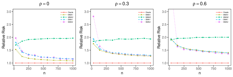
(a) $\alpha_{1}=0.51$

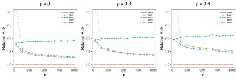
(b) $\alpha_{1}=1$

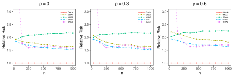
(c) $\alpha_{1}=1.5$

Figure 1: Relative risks of the competing methods in Case 1 with $\alpha_{1}=0.51$ in row (a), $\alpha_{1}=1$ in row (b), and $\alpha_{1}=1.5$ in row (c).

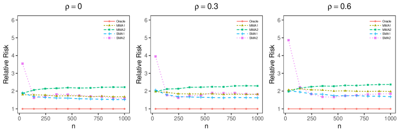
(a) $\alpha_{2}=0.5$

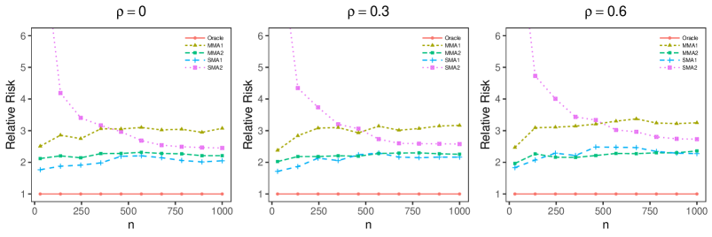
(b) $\alpha_{2}=1$

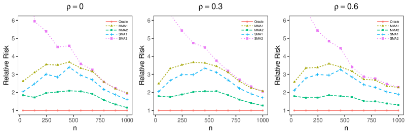
(c) $\alpha_{2}=1.5$

Figure 2: Relative risks of the competing methods in Case 2 with $\alpha_{2}=0.5$ in row (a), $\alpha_{2}=1$ in row (b), and $\alpha_{2}=1.5$ in row (c).

From Figure 1, we observe that the relative risks of the methods MMA1, SMA1, and SMA2 gradually decrease and approach 1 with increasing $n$ in Case 1, which supports the asymptotic optimality results in this paper and the work of Peng et al., (2023). In contrast, the curves of the MMA2 method are flat and have values around 2. This result may be explained by the fact that the MMA2 method tends to assign more weights to small models due to its strong penalty, while the optimal size of candidate model in Case 1 is relatively large. In addition, Figure 1 also shows that MMA1 is the best performing method when the coefficients decay slowly and the correlation between regressors is weak ($\alpha_{1}=0.51$ and $\rho=0$). However, when $\alpha_{1}$ and $\rho$ increase, two Stein-type MA estimators perform as well as or sometimes even better than MMA1 (for example, when $\alpha_{1}=1.5$ and $\rho=0.6$). Another interesting observation is that when $\alpha_{1}=1.5$, the relative risk curves of SMA2 show some fluctuations. A possible explanation for this is that SMA2 includes fewer candidate models than SMA1 and may have certain possibility of excluding important models in Case 1.

The patterns presented in Figure 2 are slightly more complicated, but they are still consistent with the current MA theories. When $\alpha_{2}=0.5$, there are slight decreases in relative risks of the Stein-type estimators, which supports their fully asymptotic optimality results in Section 4.2. But the curves of SMA2 have more fluctuations than SMA1, which occurs due to the similar reason as that in Figure 1 (c). In contrast, the curves of MMA1 level off with relative risks significantly larger than 1. This result corroborates the findings in Peng et al., (2023) that MMA1 achieves the fully asymptotic optimality when $\alpha_{2}<1/3$ but may not when the coefficients decay too fast.

When $\alpha_{2}=1$, it can be seen from Figure 2 (b) that the relative risk of SMA2 declines steadily from 9.39 to 2.57 when $\rho=0.3$, whereas the curve of SMA1 increases slightly from 1.71 to 2.16. This finding is consistent with our theoretical understanding in Corollary 1 that SMA2 achieves the fully asymptotic optimality in a broader parameter space than SMA1. On the other hand, SMA2 actually performs much worse than SMA1, especially when $n\leq 500$. Thus, it also illustrates that the asymptotic optimality should not be the sole justification for a MA method. As shown in Figure 2 (b), the estimator with satisfactory asymptotic property (SMA2) may converge slowly and perform worse in the finite sample setting. When $\alpha_{2}=1.5$, the coefficients decay extremely fast and, MA does not have any real benefit compared to MS (Peng and Yang,, 2022). Such a case is close to the setting where a fixed-dimension true model exists. In this case, the MMA2 method becomes the best. This result is expected and in accord with the theory in Zhang et al., (2020).

One unanticipated result in Figure 2 (c) is that the relative risks of MMA1 and SMA1 experience a two-phase process, a sharp increase as the sample size $n$ is less than 500, followed by a decrease as $n$ goes above 500. Similar simulation results have also appeared in Peng et al., (2023). The existing theories cannot fully explain this phenomenon, but it might be related to the specific expression of the relative risk in the finite sample setting. Take the SMA1 method for instance. If the upper bound in (4.10) is tight, then we may assume that the exact risk of SMA1 is $C_{1}(\log n)^{2/3}+C_{2}\log n+C_{3}$, where $C_{1}\to 1$ as $n\to\infty$, and $C_{2}$ and $C_{3}$ are two positive constants. Thus, the relative risk of SMA1 is $\mbox{RE}(n)=C_{1}+C_{2}(\log n)^{1/3}+C_{3}(\log n)^{-2/3}$, which increases to $\infty$ as $n\to\infty$. However, in the finite sample setting, the monotonicity of $\mbox{RE}(n)$ may depend on the speed of $C_{1}+C_{3}(\log n)^{-2/3}$ decreasing to 1. When the decrement of $C_{1}+C_{3}(\log n)^{-2/3}$ exceeds the increment of $C_{2}(\log n)^{1/3}$ in some range of $n$, the relative risk of SMA1 shows a downward trend and vice versa.

6 Discussion

This paper establishes an explicit link between MA and shrinkage in a multiple model setting, which significantly enhances the previous understanding of the relationship between MA and shrinkage in the two-model settings. Building upon the established connections, we extend the penalized blockwise Stein rule to the linear regression setting to develop the asymptotically optimal MA estimators. We provide some specific candidate model sets on which the proposed Stein-type MA estimator achieves the performance of the optimal convex combination of all the nested models (i.e., the fully asymptotic optimality). The improvement of the proposed Stein-type MA over the existing MA approaches is illustrated theoretically and numerically. Note that a limitation of our Stein-type MA method is that it requires the variance of the error terms to be known. Thus, extending our results to the case of unknown variance is a pressing topic for future research.

The unveiled connections between MA and shrinkage offer the possibility of novel methodological developments in the area of MA. The focus of this paper has been on a linear regression setting. It is of great interest to bridge the gap between MA and shrinkage in the generalized linear model setting, and then apply the Stein estimators in some general distribution families (e.g., see Chapter 5 of Hoffmann,, 2000, for a review) to combine models. In addition, given the approximate and exact distributions of the Stein-type estimators (Ullah,, 1982; Phillips,, 1984) and the techniques of constructing Stein-type confidence intervals (Hwang and Casella,, 1982; He,, 1992), it is greatly desirable to conduct inference for the asymptotically optimal MA estimators. Note that Hansen, (2014) and Zhang and Liu, (2019) have previously investigated the inference of MA but without the asymptotic optimality results. Another research direction is building a unified theory for Bayesian and frequentist MA. Indeed, the BIC weighting method considered in the frequentist literature (Buckland et al.,, 1997; Hjort and Claeskens,, 2003) can be seen as an approximation of Bayesian MA. We conjecture that the asymptotically optimal MA estimator may also have a Bayesian interpretation since the Stein-type estimation is essentially an empirical Bayes approach (see, e.g., Efron and Morris,, 1973). We leave these for future work.

Appendix A.1 Proof of Proposition 1

We first introduce some notations. Given a candidate model set $\mathcal{M}=\{k_{1},k_{2},\ldots,k_{M_{n}}\}$, define $\mathcal{M}_{1}=\mathcal{M}$. For $t\geq 1$, define

$$\mathcal{M}_{t+1}=\mathcal{M}_{t}\setminus\{s_{t,l}:l\in\mathcal{I}_{t}\},$$ (A.1.1)

where $s_{t,l}$ is the size of the $l$-th smallest model in $\mathcal{M}_{t}$. If $|\mathcal{M}_{t}|>2$ and there exists an $l\in\{2,\ldots,|\mathcal{M}_{t}|-1\}$ such that $\|\bm{\mu}_{l|\mathcal{M}_{t}}\|^{2}/\sigma^{2}_{l|\mathcal{M}_{t}}<\|\bm{\mu}_{l+1|\mathcal{M}_{t}}\|^{2}/\sigma^{2}_{l+1|\mathcal{M}_{t}}$, then define

$$\mathcal{I}_{t}=\left\{l\in\left\{2,\ldots,|\mathcal{M}_{t}|-1\right\}:\|\bm{\mu}_{l|\mathcal{M}_{t}}\|^{2}/\sigma^{2}_{l|\mathcal{M}_{t}}<\|\bm{\mu}_{l+1|\mathcal{M}_{t}}\|^{2}/\sigma^{2}_{l+1|\mathcal{M}_{t}}\right\}.$$

Otherwise, if $\mathcal{M}_{t}=\{k_{1},k_{M_{n}}\}$ or for any $l\in\{2,\ldots,|\mathcal{M}_{t}|-1\}$, $\|\bm{\mu}_{l|\mathcal{M}_{t}}\|^{2}/\sigma^{2}_{l|\mathcal{M}_{t}}\geq\|\bm{\mu}_{l+1|\mathcal{M}_{t}}\|^{2}/\sigma^{2}_{l+1|\mathcal{M}_{t}}$, then define $\mathcal{I}_{t}=\emptyset$. Let $T=\arg\min_{t}\{\mathcal{I}_{t}=\emptyset\}$ and define $\mathcal{M}_{T}=\{s_{T,1},\ldots,s_{T,|\mathcal{M}_{T}|}\}$, where $s_{T,l}$ is the size of the $l$-th smallest model in $\mathcal{M}_{T}$. $\mathcal{M}_{T}$ is actually the largest subset $\mathcal{S}$ of $\mathcal{M}$ satisfying $\|\bm{\mu}_{l|\mathcal{S}}\|^{2}/\sigma^{2}_{l|\mathcal{S}}\geq\|\bm{\mu}_{l+1|\mathcal{S}}\|^{2}/\sigma^{2}_{l+1|\mathcal{S}}$.

From (3.3), we have

$$\begin{split}&R_{n}(\mathbf{w}|\mathcal{M},\bm{\mu})=R_{n}(\bm{\gamma}|\mathcal{M},\bm{\mu})\\ &=\sum_{m=1}^{M_{n}}\left(\|\bm{\mu}_{m|\mathcal{M}}\|^{2}+\sigma^{2}_{m|\mathcal{M}}\right)\left[\gamma_{m}-\frac{\|\bm{\mu}_{m|\mathcal{M}}\|^{2}}{\|\bm{\mu}_{m|\mathcal{M}}\|^{2}+\sigma^{2}_{m|\mathcal{M}}}\right]^{2}\\ &\quad+\sum_{m=1}^{M_{n}}\frac{\|\bm{\mu}_{m|\mathcal{M}}\|^{2}\sigma^{2}_{m|\mathcal{M}}}{\|\bm{\mu}_{m|\mathcal{M}}\|^{2}+\sigma^{2}_{m|\mathcal{M}}}+\|\bm{\mu}_{M_{n}+1|\mathcal{M}}\|^{2}.\end{split}$$ (A.1.2)

Since $0\leq\|\bm{\mu}_{m|\mathcal{M}}\|^{2}/(\|\bm{\mu}_{m|\mathcal{M}}\|^{2}+\sigma^{2}_{m|\mathcal{M}})\leq 1$, the optimal MA risk in the enlarged weight set $\widetilde{\mathcal{W}}_{M_{n}}$ is

$$\begin{split}R_{n}(\widetilde{\mathbf{w}}^{*}|\mathcal{M},\bm{\mu})&=\min_{\mathbf{w}\in\widetilde{\mathcal{W}}_{M_{n}}}R_{n}(\mathbf{w}|\mathcal{M},\bm{\mu})=\min_{\bm{\gamma}\in\widetilde{\Gamma}_{M_{n}}}R_{n}(\bm{\gamma}|\mathcal{M},\bm{\mu})\\ &=\sum_{m=1}^{M_{n}}\frac{\|\bm{\mu}_{m|\mathcal{M}}\|^{2}\sigma^{2}_{m|\mathcal{M}}}{\|\bm{\mu}_{m|\mathcal{M}}\|^{2}+\sigma^{2}_{m|\mathcal{M}}}+\|\bm{\mu}_{M_{n}+1|\mathcal{M}}\|^{2}.\end{split}$$

Now our main task is to calculate $R_{n}(\mathbf{w}^{*}|\mathcal{M},\bm{\mu})=\min_{\bm{\gamma}\in\Gamma_{M_{n}}}R_{n}(\bm{\gamma}|\mathcal{M},\bm{\mu})$, where $\Gamma_{M_{n}}$ is defined in (3.4). The monotonicity of the sequence $\{\|\bm{\mu}_{m|\mathcal{M}}\|^{2}/\sigma^{2}_{m|\mathcal{M}}\}_{m=1}^{M_{n}}$ plays a key role in the optimal MA risk $R_{n}(\mathbf{w}^{*}|\mathcal{M},\bm{\mu})$. When $\{\|\bm{\mu}_{m|\mathcal{M}}\|^{2}/\sigma^{2}_{m|\mathcal{M}}\}_{m=1}^{M_{n}}$ is monotonically non-increasing, we see that $\|\bm{\mu}_{m|\mathcal{M}}\|^{2}/(\|\bm{\mu}_{m|\mathcal{M}}\|^{2}+\sigma^{2}_{m|\mathcal{M}})$ is also monotonically non-increasing. In view of (A.1.2), the optimal MA risk in $\Gamma_{M_{n}}$ is given by

$$R_{n}(\mathbf{w}^{*}|\mathcal{M},\bm{\mu})=\frac{\sigma^{4}_{1|\mathcal{M}}}{\|\bm{\mu}_{1|\mathcal{M}}\|^{2}+\sigma^{2}_{1|\mathcal{M}}}+\sum_{m=1}^{M_{n}}\frac{\|\bm{\mu}_{m|\mathcal{M}}\|^{2}\sigma^{2}_{m|\mathcal{M}}}{\|\bm{\mu}_{m|\mathcal{M}}\|^{2}+\sigma^{2}_{m|\mathcal{M}}}+\|\bm{\mu}_{M_{n}+1|\mathcal{M}}\|^{2}.$$

In contrast, if the sequence $\{\|\bm{\mu}_{m|\mathcal{M}}\|^{2}/\sigma^{2}_{m|\mathcal{M}}\}_{m=1}^{M_{n}}$ is not strictly monotone non-increasing, let

$$\mathcal{I}_{1}=\left\{l\in\left\{2,\ldots,M_{n}-1\right\}:\|\bm{\mu}_{l|\mathcal{M}}\|^{2}/\sigma^{2}_{l|\mathcal{M}}<\|\bm{\mu}_{l+1|\mathcal{M}}\|^{2}/\sigma^{2}_{l+1|\mathcal{M}}\right\}$$

denote the set of indexes where the monotonicity is violated. Based on (A.1.2), we see that minimizing $R_{n}(\bm{\gamma}|\mathcal{M},\bm{\mu})$ over $\Gamma_{M_{n}}$ is equivalent to minimizing $R_{n}(\bm{\gamma}|\mathcal{M},\bm{\mu})$ over

$$\Gamma_{M_{n},(1)}=\left\{\bm{\gamma}\in\Gamma_{M_{n}}:\gamma_{l}=\gamma_{l+1},l\in\mathcal{I}_{1}\right\}.$$ (A.1.3)

It is immediate to observe that

$$R_{n}(\mathbf{w}^{*}|\mathcal{M},\bm{\mu})=\min_{\bm{\gamma}\in\Gamma_{M_{n},(1)}}R_{n}(\bm{\gamma}|\mathcal{M},\bm{\mu})=\min_{\bm{\gamma}\in\Gamma_{|\mathcal{M}_{2}|}}R_{n}(\bm{\gamma}|\mathcal{M}_{(2)},\bm{\mu}),$$ (A.1.4)

where $\mathcal{M}_{2}$ is defined in (A.1.1), and the second equality is due to the fact that the adding the additional equality constraint on $\bm{\gamma}$ is equivalent to merging the candidate models. If the monotonicity assumption is still violated based on $\mathcal{M}_{2}$, then we repeat the above process $T-2$ times until obtaining a $\mathcal{M}_{T}$, where all elements in $\{\|\bm{\mu}_{m|\mathcal{M}_{T}}\|^{2}/\sigma^{2}_{m|\mathcal{M}_{T}}\}_{m=2}^{|\mathcal{M}_{T}|}$ are monotonically non-increasing. This completes the proof.

Appendix A.2 Proof of Theorem 1

The proof of this theorem basically follows the same lines as the proofs in Cavalier and Tsybakov, (2001, 2002) but involves additional complexity since the covariances of $\bm{\varepsilon}_{m|\mathcal{M}}$, $m=1,\ldots,M_{n}$ are not identity matrixes.

We lower bound the optimal MA risk by

$$\begin{split}R_{n}(\mathbf{w}^{*}|\mathcal{M},\bm{\mu})&\geq\sum_{m=1}^{M_{n}}\min_{\gamma_{m}}\left[\|\bm{\mu}_{m|\mathcal{M}}\|^{2}(1-\gamma_{m})^{2}+\sigma^{2}_{m|\mathcal{M}}\gamma_{m}^{2}\right]+\|\bm{\mu}_{M_{n}+1|\mathcal{M}}\|^{2}\\ &=\sum_{m=1}^{M_{n}}\frac{\sigma^{2}_{m|\mathcal{M}}\|\bm{\mu}_{m|\mathcal{M}}\|^{2}}{\sigma^{2}_{m|\mathcal{M}}+\|\bm{\mu}_{m|\mathcal{M}}\|^{2}}+\|\bm{\mu}_{M_{n}+1|\mathcal{M}}\|^{2}.\end{split}$$ (A.2.1)

The risk of the Stein-type MA estimator is

$$\mathbb{E}L_{n}(\widehat{\mathbf{w}}|\mathcal{M},\bm{\mu})=\sum_{m=1}^{M_{n}}\mathbb{E}\|\widehat{\gamma}_{m}\mathbf{y}_{m|\mathcal{M}}-\bm{\mu}_{m|\mathcal{M}}\|^{2}+\|\bm{\mu}_{M_{n}+1|\mathcal{M}}\|^{2}.$$ (A.2.2)

The task now is to find the upper bounds of $\mathbb{E}\|\widehat{\gamma}_{m}\mathbf{y}_{m|\mathcal{M}}-\bm{\mu}_{m|\mathcal{M}}\|^{2}$, $m=1,\ldots,M_{n}$, respectively. Following Cavalier and Tsybakov, (2002), we consider two different cases:

$$\|\bm{\mu}_{m|\mathcal{M}}\|^{2}<\varphi_{m}\sigma^{2}_{m|\mathcal{M}}/2,$$ (A.2.3)

and

$$\|\bm{\mu}_{m|\mathcal{M}}\|^{2}\geq\varphi_{m}\sigma^{2}_{m|\mathcal{M}}/2.$$ (A.2.4)

We first construct the upper bound for $\mathbb{E}\|\widehat{\gamma}_{m}\mathbf{y}_{m|\mathcal{M}}-\bm{\mu}_{m|\mathcal{M}}\|^{2}$ under (A.2.3). Note that

$$\begin{split}\mathbb{E}\|\widehat{\gamma}_{m}\mathbf{y}_{m|\mathcal{M}}-\bm{\mu}_{m|\mathcal{M}}\|^{2}&=\mathbb{E}\|(\widehat{\gamma}_{m}-1)\mathbf{y}_{m|\mathcal{M}}+\bm{\varepsilon}_{m|\mathcal{M}}\|^{2}\\ &=\mathbb{E}\|\bm{\varepsilon}_{m|\mathcal{M}}\|^{2}+2\mathbb{E}\left\langle(\widehat{\gamma}_{m}-1)\mathbf{y}_{m|\mathcal{M}},\bm{\varepsilon}_{m|\mathcal{M}}\right\rangle+\mathbb{E}\|(\widehat{\gamma}_{m}-1)\mathbf{y}_{m|\mathcal{M}}\|^{2}.\end{split}$$ (A.2.5)

The first term $\mathbb{E}\|\bm{\varepsilon}_{m|\mathcal{M}}\|^{2}=\sigma^{2}_{m|\mathcal{M}}$. For the second term, we obtain

$$\mathbb{E}\left\langle(\widehat{\gamma}_{m}-1)\mathbf{y}_{m|\mathcal{M}},\bm{\varepsilon}_{m|\mathcal{M}}\right\rangle=\mathbb{E}\left[\sum_{i=1}^{n}(\widehat{\gamma}_{m}-1)y_{m|\mathcal{M},i}\varepsilon_{m|\mathcal{M},i}\right],$$ (A.2.6)

where $y_{m|\mathcal{M},i}$, $\mu_{m|\mathcal{M},i}$, and $\varepsilon_{m|\mathcal{M},i}$ denote the $i$-th elements of $\mathbf{y}_{m|\mathcal{M}}$, $\bm{\mu}_{m|\mathcal{M}}$, and $\bm{\varepsilon}_{m|\mathcal{M}}$, respectively.

Define $A_{m|\mathcal{M}}$ the event $\{\|\mathbf{y}_{m|\mathcal{M}}\|^{2}\geq\sigma^{2}_{m|\mathcal{M}}(1+\varphi_{m})\}$. Based on Lemma 1 of Liu, (1994), we have

$$\begin{split}&\mathbb{E}\left[(\widehat{\gamma}_{m}-1)y_{m|\mathcal{M},i}\varepsilon_{m|\mathcal{M},i}\right]=\mbox{cov}\left[y_{m|\mathcal{M},i},(\widehat{\gamma}_{m}-1)y_{m|\mathcal{M},i}\right]\\ &=\sum_{j=1}^{n}\mbox{cov}(y_{m|\mathcal{M},i},y_{m|\mathcal{M},j})\mathbb{E}\left(\frac{\partial\widehat{\gamma}_{m}}{\partial y_{m|\mathcal{M},j}}y_{m|\mathcal{M},i}\right)+\mbox{var}(y_{m|\mathcal{M},i})\mathbb{E}(\widehat{\gamma}_{m}-1),\\ \end{split}$$ (A.2.7)

where

$$\frac{\partial\widehat{\gamma}_{m}}{\partial y_{m|\mathcal{M},j}}=\frac{2\sigma^{2}_{m|\mathcal{M}}(1+\varphi_{m})y_{m|\mathcal{M},j}I(A_{m|\mathcal{M}})}{\|\mathbf{y}_{m|\mathcal{M}}\|^{4}}.$$ (A.2.8)

Substituting (A.2.17)–(A.2.8) into (A.2.5) yields

$$\begin{split}&\quad\,\mathbb{E}\|\widehat{\gamma}_{m}\mathbf{y}_{m|\mathcal{M}}-\bm{\mu}_{m|\mathcal{M}}\|^{2}=\sigma^{2}_{m|\mathcal{M}}\\ &+\mathbb{E}\left\{\frac{4\sigma^{2}_{m|\mathcal{M}}(1+\varphi_{m})I(A_{m|\mathcal{M}})}{\|\mathbf{y}_{m|\mathcal{M}}\|^{4}}\sum_{i=1}^{n}\sum_{j=1}^{n}\mbox{cov}(y_{m|\mathcal{M},i},y_{m|\mathcal{M},j})y_{m|\mathcal{M},i}y_{m|\mathcal{M},j}\right\}\\ &-2\mathbb{E}\left[\frac{\sigma^{2}_{m|\mathcal{M}}(1+\varphi_{m})I(A_{m|\mathcal{M}})}{\|\mathbf{y}_{m|\mathcal{M}}\|^{2}}+I(\bar{A}_{m|\mathcal{M}})\right]\sum_{i=1}^{n}\mbox{var}(y_{m|\mathcal{M},i})\\ &+\mathbb{E}\left[\frac{\sigma^{4}_{m|\mathcal{M}}(1+\varphi_{m})^{2}I(A_{m|\mathcal{M}})}{\|\mathbf{y}_{m|\mathcal{M}}\|^{2}}+\|\mathbf{y}_{m|\mathcal{M}}\|^{2}I(\bar{A}_{m|\mathcal{M}})\right].\end{split}$$ (A.2.9)

Since $\sum_{i=1}^{n}\mbox{var}(y_{m|\mathcal{M},i})=\sigma^{2}_{m|\mathcal{M}}$ and

$$\begin{split}&\sum_{i=1}^{n}\sum_{j=1}^{n}\mbox{cov}(y_{m|\mathcal{M},i},y_{m|\mathcal{M},j})y_{m|\mathcal{M},i}y_{m|\mathcal{M},j}=\sigma^{2}\mathbf{y}_{m|\mathcal{M}}^{\top}\mathbf{D}_{m|\mathcal{M}}\mathbf{y}_{m|\mathcal{M}}\leq\sigma^{2}\|\mathbf{y}_{m|\mathcal{M}}\|^{2},\end{split}$$ (A.2.10)

we have

$$\mathbb{E}\|\widehat{\gamma}_{m}\mathbf{y}_{m|\mathcal{M}}-\bm{\mu}_{m|\mathcal{M}}\|^{2}\leq\|\bm{\mu}_{m|\mathcal{M}}\|^{2}+\mathbb{E}\left[W(\|\mathbf{y}_{m|\mathcal{M}}\|^{2})I(A_{m|\mathcal{M}})\right],$$ (A.2.11)

where $W(x)$ is the function

$$W(x)=-x+2\sigma^{2}_{m|\mathcal{M}}+\frac{\sigma^{4}_{m|\mathcal{M}}\left[4(1+\varphi_{m})/(k_{m}-k_{m-1})-(1-\varphi_{m}^{2})\right]}{x}.$$ (A.2.12)

Then following the proofs in the Proposition 1 of Cavalier and Tsybakov, (2002), we see that under the condition (A.2.3),

$$\mathbb{E}\|\widehat{\gamma}_{m}\mathbf{y}_{m|\mathcal{M}}-\bm{\mu}_{m|\mathcal{M}}\|^{2}\leq\frac{1}{1-\varphi_{m}/2}\frac{\sigma^{2}_{m|\mathcal{M}}\|\bm{\mu}_{m|\mathcal{M}}\|^{2}}{\sigma^{2}_{m|\mathcal{M}}+\|\bm{\mu}_{m|\mathcal{M}}\|^{2}}+\frac{8\sigma^{2}_{m|\mathcal{M}}}{k_{m}-k_{m-1}}\exp\left[-\frac{(k_{m}-k_{m-1})\varphi_{m}^{2}}{16(1+2\sqrt{\varphi_{m}})^{2}}\right].$$ (A.2.13)

Then, we construct the upper bound under (A.2.4). From Theorem 6.2 of Lehmann, (1983), it is evident that

$$\mathbb{E}\|\widehat{\gamma}_{m}\mathbf{y}_{m|\mathcal{M}}-\bm{\mu}_{m|\mathcal{M}}\|^{2}\leq\mathbb{E}\|\widetilde{\gamma}_{m}\mathbf{y}_{m|\mathcal{M}}-\bm{\mu}_{m|\mathcal{M}}\|^{2},$$ (A.2.14)

where

$$\widetilde{\gamma}_{m}=1-\frac{\sigma_{m|\mathcal{M}}^{2}(1+\varphi_{m})}{\|\mathbf{y}_{m|\mathcal{M}}\|^{2}}$$ (A.2.15)

Similar to (A.2.5), we have

$$\begin{split}\mathbb{E}\|\widetilde{\gamma}_{m}\mathbf{y}_{m|\mathcal{M}}-\bm{\mu}_{m|\mathcal{M}}\|^{2}&=\mathbb{E}\|(\widetilde{\gamma}_{m}-1)\mathbf{y}_{m|\mathcal{M}}+\bm{\varepsilon}_{m|\mathcal{M}}\|^{2}\\ &=\mathbb{E}\|\bm{\varepsilon}_{m|\mathcal{M}}\|^{2}+2\mathbb{E}\left\langle(\widetilde{\gamma}_{m}-1)\mathbf{y}_{m|\mathcal{M}},\bm{\varepsilon}_{m|\mathcal{M}}\right\rangle+\mathbb{E}\|(\widetilde{\gamma}_{m}-1)\mathbf{y}_{m|\mathcal{M}}\|^{2}.\end{split}$$ (A.2.16)

And the second term of (A.2.16) is

$$\mathbb{E}\left\langle(\widetilde{\gamma}_{m}-1)\mathbf{y}_{m|\mathcal{M}},\bm{\varepsilon}_{m|\mathcal{M}}\right\rangle=\mathbb{E}\left[\sum_{i=1}^{n}(\widetilde{\gamma}_{m}-1)y_{m|\mathcal{M},i}\varepsilon_{m|\mathcal{M},i}\right].$$ (A.2.17)

Using Lemma 1 of Liu, (1994) again, we have

$$\begin{split}\mathbb{E}\left[(\widetilde{\gamma}_{m}-1)y_{m|\mathcal{M},i}\varepsilon_{m|\mathcal{M},i}\right]=&\sigma_{m|\mathcal{M}}^{2}(1+\varphi_{m})\sum_{j=1}^{n}\mbox{cov}(y_{m|\mathcal{M},i},y_{m|\mathcal{M},j})\mathbb{E}\left(\frac{2y_{m|\mathcal{M},i}y_{m|\mathcal{M},j}}{\|\mathbf{y}_{m|\mathcal{M}}\|^{4}}\right)\\ &-\sigma_{m|\mathcal{M}}^{2}(1+\varphi_{m})\mbox{var}(y_{m|\mathcal{M},i})\mathbb{E}\left(\frac{1}{\|\mathbf{y}_{m|\mathcal{M}}\|^{2}}\right).\end{split}$$ (A.2.18)

Therefore, we have

$$\begin{split}&\mathbb{E}\|\widetilde{\gamma}_{m}\mathbf{y}_{m|\mathcal{M}}-\bm{\mu}_{m|\mathcal{M}}\|^{2}=\sigma^{2}_{m|\mathcal{M}}+4\sigma_{m|\mathcal{M}}^{2}(1+\varphi_{m})\sum_{i=1}^{n}\sum_{j=1}^{n}\mbox{cov}(y_{m|\mathcal{M},i},y_{m|\mathcal{M},j})\mathbb{E}\left(\frac{y_{m|\mathcal{M},i}y_{m|\mathcal{M},j}}{\|\mathbf{y}_{m|\mathcal{M}}\|^{4}}\right)\\ &\quad-2\sigma_{m|\mathcal{M}}^{2}(1+\varphi_{m})\sum_{i=1}^{n}\mbox{var}(y_{m|\mathcal{M},i})\mathbb{E}\left(\frac{1}{\|\mathbf{y}_{m|\mathcal{M}}\|^{2}}\right)+\mathbb{E}\left[\frac{\|\mathbf{y}_{m|\mathcal{M}}\|^{2}\sigma_{m|\mathcal{M}}^{4}(1+\varphi_{m})^{2}}{\|\mathbf{y}_{m|\mathcal{M}}\|^{4}}\right]\\ &\leq\sigma^{2}_{m|\mathcal{M}}+4\sigma^{2}\sigma_{m|\mathcal{M}}^{2}(1+\varphi_{m})\mathbb{E}\left(\frac{1}{\|\mathbf{y}_{m|\mathcal{M}}\|^{2}}\right)-2\sigma_{m|\mathcal{M}}^{4}(1+\varphi_{m})\mathbb{E}\left(\frac{1}{\|\mathbf{y}_{m|\mathcal{M}}\|^{2}}\right)\\ &\quad+\sigma_{m|\mathcal{M}}^{4}(1+\varphi_{m})^{2}\mathbb{E}\left(\frac{1}{\|\mathbf{y}_{m|\mathcal{M}}\|^{2}}\right)\\ &=\sigma^{2}_{m|\mathcal{M}}-\left[1-\varphi_{m}^{2}-4(1+\varphi_{m})/(k_{m}-k_{m-1})\right]\sigma_{m|\mathcal{M}}^{4}\mathbb{E}\frac{1}{\|\mathbf{y}_{m|\mathcal{M}}\|^{2}}.\end{split}$$ (A.2.19)

Under Assumption 2, the second term of (A.2.19) is negative. Combining with

$$\mathbb{E}\left(\frac{1}{\|\mathbf{y}_{m|\mathcal{M}}\|^{2}}\right)\geq\frac{1}{\mathbb{E}\|\mathbf{y}_{m|\mathcal{M}}\|^{2}}=\frac{1}{\sigma^{2}_{m|\mathcal{M}}+\|\bm{\mu}_{m|\mathcal{M}}\|^{2}},$$ (A.2.20)

we have

$$\begin{split}&\mathbb{E}\|\bar{\gamma}_{m}\mathbf{y}_{m|\mathcal{M}}-\bm{\mu}_{m|\mathcal{M}}\|^{2}\\ &\leq\frac{\sigma^{2}_{m|\mathcal{M}}\|\bm{\mu}_{m|\mathcal{M}}\|^{2}}{\sigma^{2}_{m|\mathcal{M}}+\|\bm{\mu}_{m|\mathcal{M}}\|^{2}}\left[\frac{\sigma^{2}_{m|\mathcal{M}}+\|\bm{\mu}_{m|\mathcal{M}}\|^{2}}{\|\bm{\mu}_{m|\mathcal{M}}\|^{2}}-\frac{\sigma^{2}_{m|\mathcal{M}}}{\|\bm{\mu}_{m|\mathcal{M}}\|^{2}}+\frac{[\varphi_{m}^{2}+8/(k_{m}-k_{m-1})]\sigma^{2}_{m|\mathcal{M}}}{\|\bm{\mu}_{m|\mathcal{M}}\|^{2}}\right]\\ &\leq\frac{\sigma^{2}_{m|\mathcal{M}}\|\bm{\mu}_{m|\mathcal{M}}\|^{2}}{\sigma^{2}_{m|\mathcal{M}}+\|\bm{\mu}_{m|\mathcal{M}}\|^{2}}\left[1+\frac{2[\varphi_{m}^{2}+8/(k_{m}-k_{m-1})]}{\varphi_{m}^{2}}\right].\end{split}$$ (A.2.21)

In view of Assumption 2, we have

$$\frac{1}{1-\varphi_{m}/2}\leq 1+\varphi_{m}\leq 1+\frac{2\left(\varphi_{m}^{2}+8/(k_{m}-k_{m-1})\right)}{\varphi_{m}}.$$ (A.2.22)

Combining (A.2.13) with (A.2.21), we can conclude that

$$\begin{split}\mathbb{E}\|\widehat{\gamma}_{m}\mathbf{y}_{m|\mathcal{M}}-\bm{\mu}_{m|\mathcal{M}}\|^{2}&\leq\left\{(1+2\varphi_{m}+16/[(k_{m}-k_{m-1})\varphi_{m}]\right\}\frac{\sigma^{2}_{m|\mathcal{M}}\|\bm{\mu}_{m|\mathcal{M}}\|^{2}}{\sigma^{2}_{m|\mathcal{M}}+\|\bm{\mu}_{m|\mathcal{M}}\|^{2}}\\ &+\frac{8\sigma^{2}_{m|\mathcal{M}}}{k_{m}-k_{m-1}}\exp\left[-\frac{(k_{m}-k_{m-1})\varphi_{m}^{2}}{16(1+2\sqrt{\varphi_{m}})^{2}}\right]\end{split}$$ (A.2.23)

Under Assumption 1, summing up (A.2.23) yields

$$\mathbb{E}L_{n}(\widehat{\mathbf{w}}|\mathcal{M},\bm{\mu})\leq(1+\bar{\varphi})\sum_{m=1}^{M_{n}}\frac{\sigma^{2}_{m|\mathcal{M}}\|\bm{\mu}_{m|\mathcal{M}}\|^{2}}{\sigma^{2}_{m|\mathcal{M}}+\|\bm{\mu}_{m|\mathcal{M}}\|^{2}}+8c_{1}\sigma^{2}+\|\bm{\mu}_{M_{n}+1|\mathcal{M}}\|^{2},$$ (A.2.24)

where $\bar{\varphi}=\max_{1\leq m\leq M_{n}}2\varphi_{m}+16/[(k_{m}-k_{m-1})\varphi_{m}$. Substituting (A.2.24) into (A.2.1), we have proved the theorem.

Appendix A.3 Proof of Theorem 2

We first prove that

$$R_{n}(\mathbf{w}^{*}|\mathcal{M},\bm{\mu})\leq(1+\zeta_{n})R_{n}(\mathbf{w}^{*}|\mathcal{M}_{a},\bm{\mu})+k_{1}\sigma^{2}.$$ (A.3.1)

Define an $M_{n}$-dimensional weight vector $\bar{\mathbf{w}}=(\bar{w}_{1},\ldots,\bar{w}_{M_{n}})^{\top}$, where $\bar{w}_{m}=\sum_{j=k_{m-1}+1}^{k_{m}}w_{j}^{*}$, $\bar{\gamma}_{m}=\sum_{j=m}^{M_{n}}\bar{w}_{m}$, and $w_{j}^{*}$ is the $j$-th element of $\mathbf{w}^{*}|\mathcal{M}_{a}$. According to (3.3), we have

$$\begin{split}R_{n}(\bar{\mathbf{w}}|\mathcal{M},\bm{\mu})&=\sum_{m=1}^{M_{n}}\left[\|\bm{\mu}_{m|\mathcal{M}}\|^{2}(1-\bar{\gamma}_{m})^{2}+\sigma^{2}_{m|\mathcal{M}}\bar{\gamma}_{m}^{2}\right]\\ &=\sum_{m=1}^{M_{n}}\left[\sum_{j=k_{m-1}+1}^{k_{m}}\|\bm{\mu}_{j|\mathcal{M}_{a}}\|^{2}(1-\bar{\gamma}_{m})^{2}+\sigma^{2}_{m|\mathcal{M}}\bar{\gamma}_{m}^{2}\right]\\ &\leq\sum_{m=1}^{p_{n}}\|\bm{\mu}_{m|\mathcal{M}_{a}}\|^{2}(1-\gamma_{m}^{*})^{2}+\sum_{m=1}^{M_{n}}\sigma^{2}_{m|\mathcal{M}}\bar{\gamma}_{m}^{2}\end{split}$$ (A.3.2)

where the inequality follows the fact that $\gamma_{j}^{*}\leq\bar{\gamma}_{m}$ when $k_{m-1}+1\leq j\leq k_{m}$. Note that

$$\begin{split}\sum_{m=1}^{M_{n}}\sigma^{2}_{m|\mathcal{M}}\bar{\gamma}_{m}^{2}&\leq k_{1}\sigma^{2}+(1+\zeta_{n})\sum_{m=2}^{M_{n}}(k_{m-1}-k_{m-2})\sigma^{2}\bar{\gamma}_{m}^{2}\\ &\leq k_{1}\sigma^{2}+(1+\zeta_{n})\sigma^{2}\sum_{j=1}^{p_{n}}(\gamma_{j}^{*})^{2},\end{split}$$ (A.3.3)

where the second inequality is due to $\bar{\gamma}_{m}\leq\gamma_{j}^{*}$ when $k_{m-2}+1\leq j\leq k_{m-1}$. Substituting (A.3.3) into (A.3.2), we obtain (A.3.1). Then combining the oracle inequality in Theorem 1 with (A.3.1), we proof the theorem.

Appendix A.4 Proof of Corollary 1

First, it is obvious that $\mathcal{M}^{*}$ satisfies Assumption 3. We then verify Assumption 2. Note that $1/k_{1}=1/\nu_{n}$. When $2\leq m\leq M_{n}$, we have

$$k_{m}-k_{m-1}\geq\lfloor\nu_{n}\rho_{n}(1+\rho_{n})^{m-1}\rfloor\geq(1-\rho_{n})\nu_{n}\rho_{n}(1+\rho_{n})^{m-1},$$ (A.4.1)

where the first inequality is due to the definition of $\mathcal{M}^{*}$, and the second inequality follows from $\lfloor x\rfloor\geq(1-\rho_{n})x$ when $x\geq\rho_{n}^{-1}$. Thus when $2\leq m\leq M_{n}$ and $n$ is large enough, we obtain

$$\frac{1}{k_{m}-k_{m-1}}\leq\frac{1}{(1-\rho_{n})\nu_{n}\rho_{n}}=O\left(\frac{1}{\nu_{n}\rho_{n}}\right)$$ (A.4.2)

where the first inequality is due to

$$k_{m}-k_{m-1}=\lfloor\nu_{n}\rho_{n}(1+\rho_{n})^{m-1}\rfloor\geq(1-\rho_{n})\nu_{n}\rho_{n}(1+\rho_{n})^{m-1}.$$ (A.4.3)

Since $\nu_{n}\to\infty$ and $\nu_{n}\rho_{n}\to\infty$, Assumption 2 is naturally satisfied when $n$ is large than some fixed integer $N$. Combining with (4.8), we also see that $\bar{\varphi}\to 0$ as $n\to\infty$.

We now focus on Assumption 1. Because $\varphi_{m}$ is bounded and $\varphi_{m}=1/(k_{m}-k_{m-1})^{\tau}$, then there exist a constant $C_{1}$ such that

$$\exp\left[-\frac{(k_{m}-k_{m-1})\varphi_{m}^{2}}{16(1+2\sqrt{\varphi_{m}})^{2}}\right]\leq\exp\left[-C_{1}(k_{m}-k_{m-1})^{1-2\tau}\right].$$ (A.4.4)

When $m=1$, we have $\exp(-C_{1}k_{1}^{1-2\tau})\to 0$. When $m\geq 2$, using (A.4.3), we have

$$\sum_{m=2}^{M_{n}}\exp\left[-C_{1}(k_{m}-k_{m-1})^{1-2\tau}\right]\leq\sum_{m=1}^{\infty}\exp\left[-C_{1}C_{2}\left(\nu_{n}\rho_{n}(1+\rho_{n})^{m-1}\right)^{1-2\tau}\right]\to 0,$$ (A.4.5)

which meets Assumption 1. Thus, applying Theorem 2, we proof the corollary.

References

- Akaike, (1973) Akaike, H. (1973). Information theory and an extension of the maximum likelihood principle. In Petrov, B. N. and Csaki, F., editors, Proceedings of the 2nd International Symposium on Information Theory, pages 267–281, Akademiai Kiado, Budapest.
- Amit and Geman, (1997) Amit, Y. and Geman, D. (1997). Shape quantization and recognition with randomized trees. Neural Computation, 9(7):1545–1588.
- Ando and Li, (2014) Ando, T. and Li, K.-C. (2014). A model-averaging approach for high-dimensional regression. Journal of the American Statistical Association, 109(505):254–265.
- Barnard, (1963) Barnard, G. A. (1963). New methods of quality control. Journal of the Royal Statistical Society. Series A (General), 126(2):255–258.
- Bates and Granger, (1969) Bates, J. M. and Granger, C. W. J. (1969). The combination of forecasts. Journal of the Operational Research Society, 20(4):451–468.
- Bellec, (2018) Bellec, P. C. (2018). Optimal bounds for aggregation of affine estimators. The Annals of Statistics, 46(1):30–59.
- Blaker, (1999) Blaker, H. (1999). On adaptive combination of regression estimators. Annals of the Institute of Statistical Mathematics, 51(4):679–689.
- (8) Breiman, L. (1996a). Bagging predictors. Machine Learning, 24(2):123–140.
- (9) Breiman, L. (1996b). Stacked regressions. Machine Learning, 24(1):49–64.
- Buckland et al., (1997) Buckland, S. T., Burnham, K. P., and Augustin, N. H. (1997). Model selection: An integral part of inference. Biometrics, 53:603–618.
- Cavalier and Tsybakov, (2001) Cavalier, L. and Tsybakov, A. (2001). Penalized blockwise Stein’s method, monotone oracles and sharp adaptive estimation. Mathematical Methods of Statistics, 10:247–282.
- Cavalier and Tsybakov, (2002) Cavalier, L. and Tsybakov, A. (2002). Sharp adaptation for inverse problems with random noise. Probability Theory and Related Fields, 123(3):323–354.
- Dai et al., (2014) Dai, D., Rigollet, P., Xia, L., and Zhang, T. (2014). Aggregation of affine estimators. Electronic Journal of Statistics, 8(1):302 – 327.
- Dalalyan and Salmon, (2012) Dalalyan, A. S. and Salmon, J. (2012). Sharp oracle inequalities for aggregation of affine estimators. The Annals of Statistics, 40(4):2327 – 2355.
- de Laplace, (1818) de Laplace, P. S. (1818). Deuxième Supplement à la Théorie Analytique des Probabilités. Courcier, Paris.
- Donoho and Johnstone, (1995) Donoho, D. L. and Johnstone, I. M. (1995). Adapting to unknown smoothness via wavelet shrinkage. Journal of the American Statistical Association, 90(432):1200–1224.
- Draper, (1995) Draper, D. (1995). Assessment and propagation of model uncertainty. Journal of the Royal Statistical Society: Series B (Statistical Methodology), 57:45–97.
- Efron and Morris, (1973) Efron, B. and Morris, C. (1973). Stein’s estimation rule and its competitors—An empirical Bayes approach. Journal of the American Statistical Association, 68(341):117–130.
- Fang et al., (2022) Fang, F., Yuan, C., and Tian, W. (2022). An asymptotic theory for least squares model averaging with nested models. Econometric Theory, pages 1–30.
- Fletcher, (2018) Fletcher, D. (2018). Model Averaging. Springer Berlin, Heidelberg.
- Freund, (1995) Freund, Y. (1995). Boosting a weak learning algorithm by majority. Information and Computation, 121(2):256–285.
- George, (1986) George, E. I. (1986). Minimax multiple shrinkage estimation. The Annals of Statistics, 14(1):188–205.
- George and Mcculloch, (1997) George, E. I. and Mcculloch, R. E. (1997). Approaches for Bayesian variable selection. Statistica Sinica, 7:339–373.
- Green and Strawderman, (1991) Green, E. J. and Strawderman, W. E. (1991). A james-stein type estimator for combining unbiased and possibly biased estimators. Journal of the American Statistical Association, 86(416):1001–1006.
- Hansen, (2007) Hansen, B. E. (2007). Least squares model averaging. Econometrica, 75(4):1175–1189.
- Hansen, (2014) Hansen, B. E. (2014). Model averaging, asymptotic risk, and regressor groups. Quantitative Economics, 5(3):495–530.
- Hansen, (2016) Hansen, B. E. (2016). Efficient shrinkage in parametric models. Journal of Econometrics, 190(1):115–132.
- Hansen and Racine, (2012) Hansen, B. E. and Racine, J. S. (2012). Jackknife model averaging. Journal of Econometrics, 167(1):38–46.
- He, (1992) He, K. (1992). Parametric empirical Bayes confidence intervals based on James-Stein estimator. Statistics & Risk Modeling, 10(1-2):121–132.
- Hjort and Claeskens, (2003) Hjort, N. L. and Claeskens, G. (2003). Frequentist model average estimators. Journal of the American Statistical Association, 98:879–899.
- Hoeting et al., (1999) Hoeting, J. A., Madigan, D., Raftery, A. E., and Volinsky, C. (1999). Bayesian model averaging: A tutorial. Statistical Science, 14:382–417.
- Hoffmann, (2000) Hoffmann, K. (2000). Stein estimation—A review. Statistical Papers, 41:127–158.
- Hwang and Casella, (1982) Hwang, J. T. and Casella, G. (1982). Minimax confidence sets for the mean of a multivariate normal distribution. The Annals of Statistics, 10(3):868–881.
- Judge and Mittelhammer, (2004) Judge, G. G. and Mittelhammer, R. C. (2004). A semiparametric basis for combining estimation problems under quadratic loss. Journal of the American Statistical Association, 99(466):479–487.
- Kim and White, (2001) Kim, T.-H. and White, H. (2001). James-stein-type estimators in large samples with application to the least absolute deviations estimator. Journal of the American Statistical Association, 96(454):697–705.
- Kneip, (1994) Kneip, A. (1994). Ordered linear smoothers. The Annals of Statistics, pages 835–866.
- Lehmann, (1983) Lehmann, E. (1983). Theory of Point Estimation. Wiley, New York.
- Leung and Barron, (2006) Leung, G. and Barron, A. (2006). Information theory and mixing least-squares regressions. IEEE Transactions on Information Theory, 52(8):3396–3410.
- Liu, (1994) Liu, J. S. (1994). Siegel’s formula via Stein’s identities. Statistics & Probability Letters, 21(3):247–251.
- Mallows, (1973) Mallows, C. (1973). Some comments on . Technometrics, 15:661–675.
- Mittelhammer and Judge, (2005) Mittelhammer, R. C. and Judge, G. G. (2005). Combining estimators to improve structural model estimation and inference under quadratic loss. Journal of econometrics, 128(1):1–29.
- Moral-Benito, (2015) Moral-Benito, E. (2015). Model averaging in economics: An overview. Journal of Economic Surveys, 29(1):46–75.
- Nemirovski, (1998) Nemirovski, A. (1998). Lectures on probability theory and statistics. part ii: topics in non-parametric statistics. Probability Summer School, Saint Flour, Springer-Verlag, Berlin.
- Peng et al., (2023) Peng, J., Li, Y., and Yang, Y. (2023). On optimality of Mallows model averaging. arXiv preprint arXiv:2309.13239.
- Peng and Yang, (2022) Peng, J. and Yang, Y. (2022). On improvability of model selection by model averaging. Journal of Econometrics, 229(2):246–262.
- Phillips, (1984) Phillips, P. (1984). The exact distribution of the Stein-rule estimator. Journal of Econometrics, 25(1):123–131.
- Rigollet, (2012) Rigollet, P. (2012). Kullback–Leibler aggregation and misspecified generalized linear models. The Annals of Statistics, 40(2):639 – 665.
- Stein, (1981) Stein, C. M. (1981). Estimation of the mean of a multivariate normal distribution. The Annals of Statistics, 9(6):1135 – 1151.
- Timmermann, (2006) Timmermann, A. (2006). Forecast combinations. volume 1 of Handbook of Economic Forecasting, pages 135–196. Elsevier.
- Ullah, (1982) Ullah, A. (1982). The approximate distribution function of the Stein-rule estimator. Economics Letters, 10(3):305–308.
- Ullah et al., (2017) Ullah, A., Wan, A. T., Wang, H., Zhang, X., and Zou, G. (2017). A semiparametric generalized ridge estimator and link with model averaging. Econometric Reviews, 36(1-3):370–384.
- Wan et al., (2010) Wan, A. T., Zhang, X., and Zou, G. (2010). Least squares model averaging by mallows criterion. Journal of Econometrics, 156(2):277–283.
- Wang et al., (2014) Wang, Z., Paterlini, S., Gao, F., and Yang, Y. (2014). Adaptive minimax regression estimation over sparse -hulls. Journal of Machine Learning Research, 15(1):1675–1711.
- Wolpert, (1992) Wolpert, D. H. (1992). Stacked generalization. Neural Networks, 5(2):241–259.
- Xu and Zhang, (2022) Xu, W. and Zhang, X. (2022). From model selection to model averaging: A comparison for nested linear models. arXiv preprint arXiv:2202.11978.
- Yang, (2001) Yang, Y. (2001). Adaptive regression by mixing. Journal of the American Statistical Association, 96(454):574–588.
- Yang, (2003) Yang, Y. (2003). Regression with multiple candidate models: Selecting or mixing? Statistica Sinica, 13(3):783–809.
- Yang, (2004) Yang, Y. (2004). Aggregating regression procedures to improve performance. Bernoulli, 10(1):25–47.
- Yuan and Yang, (2005) Yuan, Z. and Yang, Y. (2005). Combining linear regression models: When and how? Journal of the American Statistical Association, 100(472):1202–1214.
- Zhang, (2021) Zhang, X. (2021). A new study on asymptotic optimality of least squares model averaging. Econometric Theory, 37(2):388–407.
- Zhang and Liu, (2019) Zhang, X. and Liu, C.-A. (2019). Inference after model averaging in linear regression models. Econometric Theory, 35(4):816–841.
- Zhang et al., (2013) Zhang, X., Wan, A. T., and Zou, G. (2013). Model averaging by jackknife criterion in models with dependent data. Journal of Econometrics, 174(2):82–94.
- Zhang et al., (2020) Zhang, X., Zou, G., Liang, H., and Carroll, R. J. (2020). Parsimonious model averaging with a diverging number of parameters. Journal of the American Statistical Association, 115(530):972–984.