Bicriteria Approximation Algorithms for the Submodular Cover Problem

Abstract

In this paper, we consider the optimization problem Submodular Cover (SCP), which is to find a minimum cardinality subset of a finite universe $U$ such that the value of a submodular function $f$ is above an input threshold $\tau$. In particular, we consider several variants of SCP including the general case, the case where $f$ is additionally assumed to be monotone, and finally the case where $f$ is a regularized monotone submodular function. Our most significant contributions are that: (i) We propose a scalable algorithm for monotone SCP that achieves nearly the same approximation guarantees as the standard greedy algorithm in significantly faster time; (ii) We are the first to develop an algorithm for general SCP that achieves a solution arbitrarily close to being feasible; and finally (iii) we are the first to develop algorithms for regularized SCP. Our algorithms are then demonstrated to be effective in an extensive experimental section on data summarization and graph cut, two applications of SCP.

1 Introduction

Submodularity captures a diminishing returns property of set functions: Let $f:2^{U}\to\mathbb{R}$ be defined over subsets of a universe $U$ of size $n$. Then $f$ is submodular if for all $A\subseteq B\subseteq U$ and $x\notin B$, $f(A\cup\{x\})-f(A)\geq f(B\cup\{x\})-f(B)$. Examples of submodular set functions include cut functions in graphs [Balkanski et al., 2018], information-theoretic quantities like entropy and mutual information [Iyer et al., 2021], determinantal point processes [Gillenwater et al., 2012], and coverage functions [Bateni et al., 2017]. Submodular set functions arise in many important real-world applications including active learning [Kothawade et al., 2021, 2022], partial label learning [Bao et al., 2022], structured pruning of neural networks [El Halabi et al., 2022], data summarization [Tschiatschek et al., 2014], and client selection in federated learning [Balakrishnan et al., 2022].

While the majority of existing work has focused on developing approximation algorithms to maximize a submodular function subject to some constraint [Nemhauser et al., 1978a, Mirzasoleiman et al., 2015a, Harshaw et al., 2019, Buchbinder et al., 2014], in this paper we focus on developing algorithms for the related optimization problem of Submodular Cover (SCP), defined as follows.

Problem 1 (Submodular Cover (SCP)).

Let $f:2^{U}\to\mathbb{R}_{\geq 0}$ be a nonnegative submodular set function defined over subsets of the ground set $U$ of size $n$. Given threshold $\tau$, SCP is to find $\text{argmin}\{|X|:f(X)\geq\tau\}$ if such a set exists.

SCP captures applications where we seek to achieve a certain value of $f$ in as few elements as possible. For example, consider data summarization, where a submodular function $f$ is formulated to measure how effectively a subset $X$ summarizes the entire dataset $U$ [Tschiatschek et al., 2014]. Then if we set $\tau=\max\{f(X):X\subseteq U\}$, SCP asks to find the set of minimum size in $U$ that achieves the maximum effectiveness as a summary. Another example is when expected advertising revenue functions are formulated over subsets of a social network [Hartline et al., 2008], then SCP asks how we can reach a certain amount of revenue while picking as small a subset of users as possible.

In this paper, we propose and analyze algorithms for several variants of SCP including the general case, the case where $f$ is assumed to be monotone, and finally when $f$ is a regularized monotone submodular function (and potentially takes on negative values). In particular, the contributions of this paper are:

• We first address the need for scalable algorithms for SCP where $f$ is assumed to be monotone. While the greedy algorithm finds the best possible approximation guarantee for monotone SCP (MSCP) [Feige, 1998], it makes $O(n^{2})$ queries of $f$ which may be impractical in many applications. We propose and introduce two algorithms for MSCP which achieve nearly the same theoretical guarantee as the greedy algorithm but only make $O(n\ln(n))$ queries of $f$. In addition, we extend the work of Iyer and Bilmes [2013a] to a method of converting fast randomized approximation algorithms for the dual cardinality constrained monotone submodular maximization problem (MSMP) into approximation algorithms for MSCP.

• Next, we address the need for algorithms that can produce nearly feasible solutions to the general SCP problem. In particular, we provide the first algorithm for SCP that, with input $\epsilon>0$, returns a solution $S$ that is guaranteed to satisfy: (i) $f(S)\geq(1-\epsilon)\tau$; and (ii) $|S|=O(|OPT|/\epsilon)$ where $OPT$ is an optimal solution to the instance. A caveat for our algorithm is that it is not necessarily polynomial time and requires an exact solution to SMP on an instance of size $O(|OPT|/\epsilon^{2})$.

• Third, we are the first to consider regularized SCP (RSCP). RSCP is where the objective $f=g-c$ where $g$ is a nonnegative, monotone, and submodular function and $c$ is a modular cost penalty function. $f$ is not necessarily monotone but potentially takes on negative values, and therefore this new problem doesn’t fall under the general SCP problem. We develop a method of converting algorithms for the dual regularized submodular maximization problem [Harshaw et al., 2019] into ones for RSCP. We then propose the first algorithm for RSCP, which is a greedy algorithm using queries to a distorted version of $f=g-c$.

• Finally, we conduct an experimental analysis for our algorithms for MSCP and general SCP on instances of data summarization and graph cut. We find that our algorithms for MSCP makes a large speedup compared to the standard greedy approach, and we explore the pros and cons of each relative to the other. We also find that our algorithm for general SCP is practical for our applications despite not being guaranteed to run in polynomially many queries of $f$.

A table summarizing all of our algorithmic contributions can be found in the appendix. We now provide a number of preliminary definitions and notations that will be used throughout the paper.

1.1 Preliminary definitions

We first provide a number of prelimary definitions that will be used throughout the paper: (i) The Submodular Maximization Problem (SMP) is the dual optimization problem to SCP defined by, given budget $\kappa$, find $\text{argmax}\{f(X):X\subseteq U,|X|\leq\kappa\}$; (ii) Monotone SCP (MSCP) is the version of SCP where $f$ is additionally assumed to be monotone; (iii) Regularized SCP (RSCP) is a related problem to SCP where $f=g-c$ and $g$ is monotone, submodular, and nonnegative, while $c$ is a modular nonnegative cost function; (iv) $OPT$ is used to refer to the optimal solution to the instance of SCP that should be clear from the context; (v) $OPT_{SM}$ is used to refer to the optimal solution to the instance of SMP that should be clear from the context; (vi) An $(\alpha,\beta)$-bicriteria approximation algorithm for SCP returns a solution $X$ such that $|X|\leq\alpha|OPT|$ and $f(X)\geq\beta\tau$. An $(\alpha,\beta)$-bicriteria approximation algorithm for SMP returns a solution $X$ such that $f(X)\geq\alpha f(OPT)$ and $|X|\leq\beta\kappa$. Notice that the approximation on the objective is first, and the approximation on the constraint is second; (vii) The marginal gain of adding an element $u\in U$ to a set $S\subseteq U$ is denoted as $\Delta f(S,u)=f(S\cup u)-f(S)$; (viii) The function $f_{\tau}=\min\{f,\tau\}$.

1.2 Related Work

MSCP is the most studied variant of SCP [Wolsey, 1982, Wan et al., 2010, Mirzasoleiman et al., 2015b, 2016, Crawford et al., 2019]. The standard greedy algorithm produces a logarithmic approximation guarantee for MSCP in $O(n^{2})$ queries of $f$ [Wolsey, 1982], and this is the best approximation guarantee that we can expect unless NP has $n^{\mathcal{O}(\log(\log(n)))}$-time deterministic algorithms [Feige, 1998]. One version of the greedy algorithm for MSCP works as follows: A set $S$ is initialized to be $\emptyset$. Iteratively, the element $\text{argmax}\{\Delta f(S,x):x\in U\}$ is added to $S$ until $f(S)$ reaches $(1-\epsilon)\tau$. It has previously been shown that this is a $(\ln(1/\epsilon),1-\epsilon)$-bicriteria approximation algorithm [Krause et al., 2008]. Beyond greedy algorithms, algorithms for the distributed setting [Mirzasoleiman et al., 2015c, 2016] as well as the streaming setting [Norouzi-Fard et al., 2016] for MSCP have been proposed.

On the other hand, developing algorithms for SCP in full generality is more difficult since monotonicity of $f$ is not assumed. The standard greedy algorithm does not have any non-trivial approximation guarantee for SCP. In fact, to the best of our knowledge, no greedy-like algorithms have been found to be very useful for SCP. Recently, Crawford [2023] considered SCP and proved that it is not possible to develop an algorithm that guarantees $f(X)\geq\tau/2$ for SCP in polynomially many queries of $f$ assuming the value oracle model. On the other hand, algorithmic techniques that are used for SMP in the streaming setting [Alaluf et al., 2022] proved to be useful for SCP. In particular, Crawford [2023] proposed an algorithm using related techniques to that of Alaluf et al. that achieves a $(O(1/\epsilon^{2}),1/2-\epsilon)$-bicriteria approximation guarantee for SCP in polynomially many queries of $f$. We also take an approach inspired by the streaming algorithm of Alaluf et al., but sacrifice efficiency in order to find a solution for SCP that is arbitrarily close to being feasible.

SMP is the dual optimization problem to SCP, and has received relatively more attention than SCP [Nemhauser et al., 1978b, Badanidiyuru and Vondrák, 2014, Mirzasoleiman et al., 2015a, Feige et al., 2011, Buchbinder et al., 2014, Alaluf et al., 2022]. Iyer and Bilmes [2013b] proposed a method of converting algorithms for SMP to ones for SCP. In particular, given a deterministic $(\gamma,\beta)$-bicriteria approximation algorithm for SMP, the algorithm convert (see pseudocode in the appendix) proposed by Iyer and Bilmes produces a deterministic $((1+\alpha)\beta,\gamma)$-bicriteria approximation algorithm for SCP. The algorithm works by making $\log_{1+\alpha}(n)$ guesses for $|OPT|$ (which is unknown in SCP), running the SMP algorithm with the budget set to each guess, and returning the smallest solution with $f$ value above $\gamma\tau$. However, this approach is limited by the approximation guarantees of existing algorithms for SMP. The best $\gamma$ for monotone SMP is $1-1/e$, and the best for general SMP where $f$ is not assumed to be monotone is significantly lower [Gharan and Vondrák, 2011]. Several of the algorithms that we propose in this paper do generally follow the model of convert in that they rely on guesses of $|OPT|$, but are different because they: (i) Implicitly use bicriteria approximation algorithms for SMP which have better guarantees on the objective ($\gamma$) because they do not necessarily return a feasible solution; (ii) Are more efficient with respect to the number of queries of $f$, since convert potentially wastes many queries of $f$ by doing essentially the same behavior for different guesses of $|OPT|$.

2 Algorithms and Theoretical Guarantees

In this section, we present and theoretically analyze our algorithms for several variants of SCP. In particular, in Section 2.1 we first consider MSCP. We present a method of converting randomized algorithms for SMP to algorithms for SCP, and then we present the algorithms thresh-greedy-c and stoch-greedy-c for MSCP, which both have lower query complexity compared to the standard greedy algorithm. Next, we consider the general problem of SCP in Section 2.2. We present the algorithm stream-c for SCP, which produces a solution with $f$ value arbitrarily close to $\tau$, but does not necessarily make polynomially many queries to $f$. Finally, in Section 2.3, we consider RSCP. We present a method of converting algorithms for regularized SMP to ones for RSCP, and then introduce the algorithm distorted-bi for RSCP.

2.1 Monotone submodular cover

In this section, we develop and analyze approximation algorithms for MSCP. The greedy algorithm is a tight $(\ln(1/\epsilon),1-\epsilon)$-bicriteria approximation algorithm for MSCP [Krause et al., 2008]. However, the greedy algorithm makes $O(n^{2})$ queries of $f$, which is impractical in many application settings with large $U$ and/or when queries of $f$ are costly [Mirzasoleiman et al., 2015a]. Motivated by this, we propose and analyze the algorithms thresh-greedy-c and stoch-greedy-c for MSCP which give about the same bicriteria approximation guarantees but in many fewer queries of $f$.

We first describe thresh-greedy-c. thresh-greedy-c is closely related to the existing threshold greedy algorithm for monotone SMP [Badanidiyuru and Vondrák, 2014], and therefore we relegate the pseudocode of thresh-greedy-c to the appendix and only include a brief discussion here. At each iteration of thresh-greedy-c, instead of picking the element with highest marginal gain into $S$, it adds all elements in $U$ with marginal gain above a threshold, $w$. $w$ is initialized to $\max_{u\in U}f(\{u\})$, and is decreased by a factor of $(1-\epsilon/2)$ when the algorithm proceeds to the next iteration. thresh-greedy-c adds elements to a solution $S$ until $f(S)$ reaches $(1-\epsilon)\tau$, which is shown to happen in at most $\ln(2/\epsilon)|OPT|+1$ elements in the proof of Theorem 1. We now state the theoretical guarantees of thresh-greedy-c in Theorem 1.

Theorem 1.

thresh-greedy-c produces a solution with $(\ln(2/\epsilon)+1,1-\epsilon)$-bicriteria approximation guarantee to MSCP, in $O(\frac{n}{\epsilon}\log(\frac{n}{\epsilon}))$ number of queries of $f$.

Another method of speeding up the standard greedy algorithm is by introducing randomization, as has been done for monotone SMP in the stochastic greedy algorithm [Mirzasoleiman et al., 2015a]. A natural question is whether a randomized algorithm for monotone SMP can be converted into an algorithm for MSCP using the algorithm convert of Iyer and Bilmes. However, convert relies on a deterministic approximation guarantee. We now introduce a new algorithm called convert-rand that is analogous to convert but runs the SMP algorithm $O(\ln(n)\ln(1/\delta))$ times in order to have the approximation guarantee hold with high probability. Pseudocode for convert-rand, as well as a proof of Theorem 2 can be found in the appendix.

Theorem 2.

Any randomized $(1-\epsilon/2,\beta)$-bicriteria approximation algorithm for monotone SMP that runs in time $\mathcal{T}(n)$ where $\gamma$ holds only in expectation can be converted into a $((1+\alpha)\beta,1-\epsilon)$-bicriteria approximation algorithm for MSCP that runs in time $O(\log_{1+\alpha}(|OPT|)\ln(1/\delta)\mathcal{T}(n))$ where $\gamma$ holds with probability at least $1-\delta$.

Therefore by applying Theorem 2 to the stochastic greedy algorithm of Mirzasoleiman et al., we have a $(1+\alpha,1-1/e-\epsilon)$-bicriteria approximation algorithm for MSCP with high probability in $O(n\log_{1+\alpha}(|OPT|)\ln(1/\delta)\ln(1/\epsilon))$ queries of $f$. However, a factor of $1-1/e-\epsilon$ of $\tau$ is not very close to feasible, and further the convert-rand method wastes many queries of $f$ essentially doing the same computations for different guesses of $|OPT|$. Therefore we focus the rest of this section on developing an algorithm, stoch-greedy-c, that uses the techniques of the stochastic greedy algorithm more directly for MSCP.

The idea behind the stochastic greedy algorithm for SMP is that instead of computing the marginal gains of all elements at each iteration, we take a uniformly random sampled subset from $U$ and pick the element with the highest marginal gain among the sampled subset. If the sampled subset is sufficiently large, in particular of size at least $(n/\kappa)\ln(1/\epsilon)$ where $\kappa$ is the budget for the instance of SMP, then with high probability a uniformly random element of $OPT_{SM}$ will appear in the sampled subset and the marginal gain of adding the element is nearly the same as the standard greedy algorithm in expectation. However, in SMP we know that $|OPT_{SM}|=\kappa$, but in MSCP $|OPT|$ is unknown. Therefore it is not obvious how to apply this technique in a more direct way than convert-rand.

We now introduce our algorithm stoch-greedy-c for MSCP, pseudocode for which is provided in Algorithm 1. stoch-greedy-c takes as input $\epsilon>0$, $\delta>0$, $\alpha>0$, and an instance of MSCP. stoch-greedy-c keeps track of $O(\ln(1/\delta))$ possibly overlapping solutions $S_{1},S_{2},...$ throughout a sequence of iterations. stoch-greedy-c also keeps track of an estimate of $|OPT|$, $g$. During each iteration, for each solution $S_{i}$, stoch-greedy-c uniformly randomly and independently samples a set $R$ of size $\min\{n,(n/g)\ln(3/\epsilon)\}$ and adds $u=\text{argmax}\{\Delta f_{\tau}(S_{i},x):x\in R\}$ to $S_{i}$. Every time $\frac{\alpha}{1+\alpha}\ln(3/\epsilon)g$ elements have been added to each $S_{i}$, $g$ is increased by a factor of $1+\alpha$. stoch-greedy-c stops once there exists an $S_{i}$ such that $f(S_{i})\geq(1-\epsilon)\tau$, and returns this solution.

Algorithm 1 stoch-greedy-c

Input: $\epsilon,\alpha,\tau$
Output: $S\subseteq U$

1:$S_{i}\leftarrow\emptyset$ $\forall i\in\left\{1,...,\ln(1/\delta)/\ln(2)\right\}$

2:$r\leftarrow 1,g\leftarrow 1+\alpha$

3:while $f(S_{i})<(1-\epsilon)\tau$ $\forall i$ do

4:     for $i\in\left\{1,...,\ln(1/\delta)/\ln(2)\right\}$ do

5:          $R\leftarrow$ sample $\min\{n,n\ln(3/\epsilon)/g\}$ elements from $U$

6:         $u\leftarrow\text{argmax}_{x\in R}\Delta f_{\tau}(S_{j},x)$

7:         $S_{j}\leftarrow S_{j}\cup\{u\}$      

8:     $r\leftarrow r+1$

9:     if $r>\ln(3/\epsilon)g$ then $g\leftarrow(1+\alpha)g$     

10:return $\text{argmin}\{|S_{i}|:f(S_{i})\geq(1-\epsilon)\tau\}$

We now state the theoretical results for stoch-greedy-c in Theorem 3.

Theorem 3.

Suppose that stoch-greedy-c is run for an instance of MSCP. Then with probability at least $1-\delta$, stoch-greedy-c outputs a solution $S$ that satisfies a $((1+\alpha)\lceil\ln(3/\epsilon)\rceil,1-\epsilon)$-bicriteria approximation guarantee in at most $O\left(\frac{\alpha}{1+\alpha}n\ln(1/\delta)\ln^{2}(3/\epsilon)\log_{1+\alpha}(|OPT|)\right)$ queries of $f$.

Compared to thresh-greedy-c, stoch-greedy-c has a better dependence on $\epsilon$ in terms of the number of queries made to $f$. In addition, it is possible to extend the stochastic greedy algorithm of Mirzasoleiman et al. to a $(1-\epsilon,\ln(1/\epsilon)$-bicriteria approximation algorithm for SMP and then use convert (see the appendix). However, stoch-greedy-c still would have strictly fewer queries of $f$ by a factor of $\frac{\alpha}{1+\alpha}$ compared to this approach because convert does essentially the same computations for different guesses of $|OPT|$. In order to prove Theorem 3, we first need Lemma 1 below, which states that as long as $g\leq(1+\alpha)|OPT|$, the marginal gain of adding $u$ in Line 6 is about the same as the standard greedy algorithm in expectation.

Lemma 1.

Consider any of the sets $S_{i}$ at the beginning of an iteration on Line 4 where $g\leq(1+\alpha)|OPT|$. Then if $u_{i}$ is the random element that will be added on Line 6, we have that $\mathbb{E}[\Delta f_{\tau}(S_{i},u_{i})]\geq\frac{1-\epsilon/3}{(1+\alpha)|OPT|}(\tau-f_{\tau}(S_{i}))$.

Further, Lemma 2 below uses Lemma 1 to show that by the time $g$ reaches $(1+\alpha)|OPT|$, $\mathbb{E}[f_{\tau}(S_{i})]\geq(1-\frac{\epsilon}{2})\tau$ for all $i$.

Lemma 2.

Once $r$ reaches $(1+\alpha)\lceil\ln(3/\epsilon)|OPT|\rceil$, we have that $\mathbb{E}[f_{\tau}(S_{i})]\geq\left(1-\frac{\epsilon}{2}\right)\tau$ for all $i$.

Finally, because there are $O(\ln(1/\delta))$ solutions, by the time $g$ reaches $(1+\alpha)|OPT|$, there exists $i$ such that $f(S_{i})\geq(1-\epsilon)\tau$ with probability at least $1-\delta$ by using concentration bounds, which is stated in Lemma 3.

Lemma 3.

With probability at least $1-\delta$, once $r$ reaches $(1+\alpha)\lceil\ln(3/\epsilon)|OPT|\rceil$, we have that $\max_{i}f(S_{i})\geq(1-\epsilon)\tau$.

Lemma 3 allows us to keep increasing $g$ by a factor of $(1+\alpha)$ periodically, because intuitively the longer we keep adding elements, the bigger we know that $|OPT|$ must be since the algorithm is still running and none of the solution sets has reached $(1-\epsilon)\tau$ yet. The proof of Lemmas 1 and 2, and of Theorem 3 can be found in the appendix.

2.2 Non-monotone submodular cover

In this section, we introduce and theoretically analyze the algorithm stream-c for SCP in the general setting, where $f$ is not assumed to be monotone. In the general setting, the standard greedy algorithm doesn’t have non-trivial approximation guarantee for SCP. In addition, it has previously been shown that it is not possible for an algorithm to guarantee that $f(X)\geq\tau/2$ for SCP, where $X$ is its returned solution, in polynomially many queries of $f$ assuming the value oracle model [Crawford, 2023]. Our algorithm stream-c does produce a solution $X$ that is guaranteed to satisfy $f(X)\geq(1-\epsilon)\tau$, but relies on solving an instance of SMP exactly on a set of size $O(|OPT|/\epsilon^{2})$. Despite not being polynomial time, stream-c is practical in many instances of SCP because: (i) $|OPT|$ may be relatively small; and (ii) the instance of SMP may be relatively easy to solve, e.g. $f$ may be very close to monotone on the instance of SMP even if it was very non-monotone on the original instance of SCP. These aspects of stream-c are further explored in Section 3.

We now describe stream-c, pseudocode for which can be found in Algorithm 2. stream-c takes as input $\epsilon>0$, $\alpha>0$, and an instance of SCP. stream-c takes sequential passes through the universe $U$ (Line 4) with each pass corresponds to a new guess of $|OPT|$, $g$. $g$ is initialized as $1+\alpha$, and at the end of each pass is increased by a factor of $1+\alpha$. Throughout stream-c, a subset of elements of $U$ are stored into $2/\epsilon$ disjoint sets, $S_{1},...,S_{2/\epsilon}$. An element $u$ is stored in at most one set $S_{j}$ if both of the following are true: (i) $|S_{j}|<2g/\epsilon$; (ii) adding $u$ is sufficiently beneficial to increasing the $f$ value of $S_{j}$ i.e. $\Delta f(S_{j},u)\geq\epsilon\tau/(2g)$. If no such $S_{j}$ exists, $u$ is discarded. At the end of each pass, stream-c finds $S=\text{argmax}\{f(X):X\subseteq\cup S_{i},|X|\leq 2g/\epsilon\}$ on Line 7. If $f(S)\geq(1-\epsilon)\tau$, then $S$ is returned and stream-c terminates.

Algorithm 2 stream-c

Input: $\epsilon$, $\alpha$
Output: $S\subseteq U$

1:$S\leftarrow\emptyset,S_{1}\leftarrow\emptyset,...,S_{2/\epsilon}\leftarrow\emptyset$

2:$g\leftarrow 1+\alpha$

3:while $f(S)<(1-\epsilon)\tau$ do

4:     for $u\in U$ do

5:         if $\exists j$ s.t. $\Delta f(S_{j},u)\geq\epsilon\tau/(2g)$ and $|S_{j}|<2g/\epsilon$ then

6:              $S_{j}\leftarrow S_{j}\cup\{u\}$               

7:      $S\leftarrow\text{argmax}\{f(X):X\subseteq\cup_{i=1}^{2/\epsilon}S_{i},|X|\leq 2g/\epsilon\}$

8:     $g=(1+\alpha)g$

9:return $S$

We now present the theoretical guarantees of stream-c in Theorem 4.

Theorem 4.

Suppose that stream-c is run for an instance of SCP. Then stream-c returns $S$ such that $f(S)\geq(1-\epsilon)\tau$ and $|S|\leq(1+\alpha)(2/\epsilon)|OPT|$ in at most

$$\log_{1+\alpha}(|OPT|)\left(\frac{2n}{\epsilon}+\mathcal{T}\left((1+\alpha)\left(\frac{4}{\epsilon^{2}}|OPT|\right)\right)\right)$$

queries of $f$, where $\mathcal{T}(m)$ is the number of queries to $f$ of the algorithm for SMP used on Line 7 of Algorithm 2 on an input set of size $m$.

The key idea for proving Theorem 4 is that by the time $g$ is in the region $[|OPT|,(1+\alpha)|OPT|]$, there exists a subset $X\subseteq\cup S_{i}$ such that $|X|\leq 2g/\epsilon$ and $f(X)\geq(1-\epsilon)\tau$. In fact, it is shown in the proof of Lemma 4 in the appendix that the set $X$ is $S_{t}\cup(\cup_{i}S_{i}\cap OPT)$ for a certain one of the sets $S_{t}$. Then when we solve the instance of SMP on Line 7, we find a set that has these same properties as $X$, and stream-c returns this set and terminates. Because $g\leq(1+\alpha)|OPT|$, the properties described in Theorem 4 hold. Further notice that $|\cup_{i}S_{i}|\leq 2(1+\alpha)|OPT|/\epsilon^{2}$ at all times before stream-c exits, which implies the bounded query complexity in Theorem 4. The key idea for proving Theorem 4 is stated below in Lemma 4 and proven in the appendix.

Lemma 4.

By the time that $g$ reaches the region $[|OPT|,(1+\alpha)|OPT|]$ and the loop on Line 4 of stream-c has completed, there exists a set $X\subseteq\cup S_{i}$ of size at most $2(1+\alpha)|OPT|/\epsilon$ such that $f(X)\geq(1-\epsilon)\tau$.

2.3 Regularized monotone submodular cover

The final class of submodular functions we consider take the form $f=g-c$ where $g$ is monotone, submodular, and nonnegative, while $c$ is a modular, nonnegative penalty cost function, called RSCP. In this case, $f$ may take on negative values and therefore this class of submodular functions does not fit into general SCP. $f$ may also be nonmonotone. Existing theoretical guarantees for the dual problem of regularized SMP are in a different form than typical approximation algorithms [Harshaw et al., 2019, Kazemi et al., 2021], which we will describe in more detail below, and as a result convert cannot be used. Motivated by this, we first develop an algorithm, convert-reg, that takes algorithms for regularized SMP and converts them into an algorithm for RSCP. Next, we propose a generalization of the distorted greedy algorithm of Harshaw et al. for regularized SMP, called distorted-bi, that can be used along with convert-reg to produce an algorithm for RSCP.

Existing proposed algorithms for regularized SMP have guarantees of the following form: Given budget $\kappa$, the regularized SMP algorithm is guaranteed to return a set $S$ such that $|S|\leq\kappa$ and $g(S)-c(S)\geq\gamma g(OPT_{SM})-c(OPT_{SM})$ where $\gamma$ is some value less than 1, e.g. $1-1/e$ for the distorted greedy algorithm of Harshaw et al.. A guarantee of this form means convert cannot be used (the check on Line 2 of the pseudocode for convert in the appendix is the problem). Motivated by this, we provide convert-reg for these different types of theoretical guarantees.

We now describe convert-reg, pseudocode for which can be found in Algorithm 3. convert-reg takes as input an algorithm reg for regularized SMP, and $\alpha>0$. convert-reg repeatedly makes guesses for $|OPT|$, $\kappa$. For each guess $\kappa$, the algorithm reg is run on an instance of SMP with objective $g-(\gamma/\beta)c$ and budget $\kappa$. Once $g-(\gamma/\beta)c$ reaches $\gamma\tau$, convert-reg exits.

Algorithm 3 convert-reg

Input: $\alpha>0$
Output: $S\subseteq U$

1:$\kappa\leftarrow 1+\alpha$, $S\leftarrow\emptyset$

2:while $g(S)-\frac{\gamma}{\beta}c(S)<\gamma\tau$ do

3:     $S\leftarrow$reg run with objective $g-\frac{\gamma}{\beta}c$ and budget $\kappa$

4:     $\kappa\leftarrow(1+\alpha)\kappa$

5:return $S$

The theoretical guarantees of convert-reg are stated below in Theorem 5 and proven in the appendix. Theorem 5 makes a slightly stronger assumption on reg than its approximation guarantees relative to $OPT_{SM}$. In particular, it is assumed that it returns a solution satisfying $|S|\leq\rho\kappa$ and $g(S)-c(S)\geq\gamma g(X)-c(X)$ for all $X\subseteq U$ such that $|X|\leq\kappa$, not just for $OPT_{SM}$. However, this is true of many algorithms for regularized SMP including the distorted greedy algorithm of Harshaw et al.. The idea behind running reg with the objective $g-\frac{\gamma}{\beta}c$ instead of the actual objective $g-c$, is that by the time $\kappa$ is a good guess of $|OPT|$, it is shown in the proof of Theorem 5 that with this different objective $g(S)-\frac{\gamma}{\beta}c(S)\geq\gamma\tau$.

Theorem 5.

Suppose that we have an algorithm reg for regularized SMP, and given budget $\kappa$ reg is guaranteed to return a set $S$ of cardinality at most $\rho\kappa$ such that $g(S)-c(S)\geq\gamma g(X)-\beta c(X)$ for all $X$ such that $|X|\leq\kappa$, in time $T(n)$. Then the algorithm convert-reg using reg as a subroutine returns a set $S$ in time $O(\log_{1+\alpha}(n)T(n))$ such that $|S|\leq(1+\alpha)\rho|OPT|$ and $g(S)-\frac{\gamma}{\beta}c(S)\geq\gamma\tau.$

If we use convert-reg on the distorted greedy algorithm of Harshaw et al., we end up with an algorithm for RSCP that is guaranteed to return a set $S$ such that $|S|\leq(1+\alpha)|OPT|$ and $g(S)-(1-1/e)c(S)\geq(1-1/e)\tau$. If we set $c=0$, then the problem setting reduces to MSCP and the distorted greedy algorithm of Harshaw et al. [2019] is equivalent to the standard greedy algorithm. However, our approximation guarantee does not reduce to the $(\ln(1/\epsilon),1-\epsilon)$-bicriteria approximation guarantee that would be preferable. A more intuitive result would be one that converges to that of the standard greedy algorithm as $c$ goes to 0. Motivated by this, we now propose an extension of the distorted greedy algorithm of Harshaw et al. [2019] for regularized SMP, distorted-bi, that accomplishes this.

We now describe distorted-bi, pseudocode for which can be found in the appendix. distorted-bi takes as input an instance of regularized SMP and $\epsilon>0$. distorted-bi is related to the standard greedy algorithm, but instead of making queries to $g-c$, distorted-bi queries a distorted version of $g-c$ that de-emphasizes $g$ compared to $c$, and evolves over time. In particular, when element $i$ is being added to the solution set, we choose the element of maximum marginal gain, provided it is positive, to the objective

$$\Phi_{i}(X)=\left(1-\frac{1}{\kappa}\right)^{\ln(1/\epsilon)\kappa-i}g(X)-c(X).$$

The theoretical guarantees of distorted-bi are now presented in Theorem 6, and the proof of Theorem 6 can be found in the appendix.

Theorem 6.

Suppose that distorted-bi is run for an instance of regularized SMP. Then distorted-bi produces a solution $S$ in $O(n\kappa\ln(1/\epsilon))$ queries of $f$ such that $|S|\leq\ln(1/\epsilon)\kappa$ and for all $X\subseteq U$ such that $|X|\leq\kappa$, $g(S)-c(S)\geq(1-\epsilon)g(X)-\ln(1/\epsilon)c(X).$

Therefore by running convert-reg with distorted-bi as a subroutine for regularized SMP, we end up with an algorithm for regularized RSCP that is guaranteed to return a set $S$ such that $|S|\leq(1+\alpha)\ln(1/\epsilon)|OPT|$ and $g(S)-(1-\epsilon)c(S)/\ln(1/\epsilon)\geq(1-\epsilon)\tau$ in $O((1+\alpha)n|OPT|\log_{1+\alpha}(n)\log(1/\epsilon))$ queries of $f$.

3 Experiments

In this section, we experimentally evaluate the algorithms proposed in Sections 2.1 and 2.2 on real instances of SCP. In particular, the emphasis of Section 3.1 is on evaluation of our algorithm stoch-greedy-c on instances of data summarization, an application of MSCP. Next, we evaluate stream-c on instances of graph cut, an application of SCP that is not monotone, in Section 3.2. Additional details about the applications, setup, and results can be found in the appendix.

3.1 Monotone submodular objective

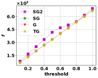
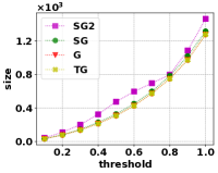
We first compare the solutions returned by stoch-greedy-c ("SG"), greedy-c ("G"), thresh-greedy-c ("TG"), and convert using the bicriteria extension of the stochastic greedy algorithm of Mirzasoleiman et al. (see appendix) ("SG2") on instances of data summarization. The data summarization instance featured here in the main paper is the delicious dataset of URLs tagged with topics, and $f$ takes a subset of URLs to the number of distinct topics represented by those URLs ($n=5000$ with $8356$ tags) [Soleimani and Miller, 2016]. Additional datasets are explored in the appendix. We run the algorithms with input $\epsilon$ in the range $(0,0.15)$ and threshold values between 0 and $f(U)$ ($f(U)$ is the total number of tags). When $\epsilon$ is varied, $\tau$ is fixed at $0.6f(U)$. When $\tau$ is varied, $\epsilon$ is fixed at $0.2$. The parameter $\alpha$ is set to be $0.1$ and the initial guess of $|OPT|$ for stoch-greedy-c and convert is set to be $\tau/\max_{s}f(s)$.

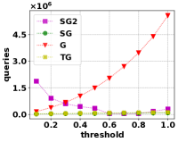
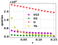
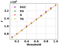
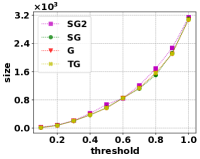
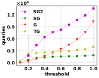
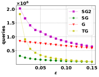
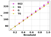
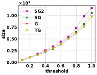
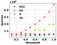
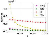
The results in terms of the $f$ values and size of the solutions are presented in Figure 1(a) and 1(b). From the plots, one can see that the $f$ values and size of solutions returned by stoch-greedy-c, greedy-c, thresh-greedy-c are nearly the same, and are smaller than the ones returned by convert. This is unsurprising, because the theoretical guarantees on $f$ and size are about the same for the different algorithms, but convert tends to perform closer to its worst case guarantee on size. The number of queries to $f$ for different $\epsilon$ and $\tau$ are depicted in Figures 1(d) and 1(c). Recall that the theoretical worst case number of queries to $f$ for stoch-greedy-c, greedy-c, thresh-greedy-c and convert are $O((\alpha/(1+\alpha))n\ln^{2}(1/\epsilon)\log_{1+\alpha}(|OPT|))$, $O(n\ln(1/\epsilon)|OPT|)$, $O(n\log(|OPT|/\epsilon)/\epsilon)$, and $O(n\ln^{2}(1/\epsilon)\log_{1+\alpha}(|OPT|)$ respectively. As expected based on these theoretical guarantees, greedy-c does the worst and increases rapidly as $\tau$ (and therefore $|OPT|$) increases. thresh-greedy-c tends to do worse compared to stoch-greedy-c and convert as $\epsilon$ gets smaller. stoch-greedy-c consistently performs the fastest out of all of the algorithms.

(a) cover $f$

(b) cover $c$

(c) cover queries

(d) cover queries

(e) euall $f$

(f) euall $c$

(g) euall queries

(h) euall queries

Figure 1: The experimental results of running the monotone algorithms on instances of data summarization on the delicious URL dataset ("cover") and running stream-c on the instances of graph cut on the email-EuAll graph ("euall").

3.2 Non-Monotone Submodular Objective

We now analyze the performance of stream-c on several instances of graph cut over real social network data. The universe $U$ is all nodes in the network, and $f$ is the number of edges between a set and its complement. The network featured in the main paper is the email-EuAll dataset ($n=265214$, 420045 edges) from the SNAP large network collection [Leskovec and Sosič, 2016] and additional datasets can be found in the appendix. We run stream-c with input $\epsilon$ in the range $(0,0.5)$ and threshold values between 0 and $f(X)$ where $X$ is a solution returned by the unconstrained submodular maximization algorithm of Buchbinder et al. [2015] on the instance. When $\epsilon$ is varied, $\tau$ is fixed at $0.9f(X)$. When $\tau$ is varied, $\epsilon$ is fixed at $0.15$.

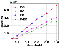
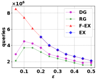
We compare the performance of stream-c using several possible algorithms for the subroutine of SMP over $\cup S_{i}$ (see line 7 in Algorithm 2), including a polynomial time approximation algorithm and an unconstrained submodular maximization algorithm. In particular, we use the random greedy approximation algorithm for SMP that is proposed in Buchbinder et al. [2014] ("RG"), and the double greedy approximation algorithm for unconstrained submodular maximization proposed in Buchbinder et al. [2015] ("DG"). Random greedy and double greedy are both approximation algorithms ($1/e$ in expectation and $1/2$ in expectation respectively), and therefore the stopping conditions are set to be $\frac{(1-\epsilon)\tau}{e}$ and $\frac{(1-\epsilon)\tau}{2}$ respectively. We also consider an exact algorithm ("EX"), which essentially is a greedy heuristic followed by an exact search of all (exponentially many) possible solutions if the greedy fails. On instances where the exact algorithm was unable to complete in a time period of $5$ minutes, we did not include a data point. We further discuss the use of these algorithms in the appendix.

Before introducing the fourth subroutine, we discuss an interesting pattern that we saw in our instances of graph cut. We noticed that it was often the case that: (i) $\cup S_{i}$ tended to be small compared to its upper bound and in fact typically $|\cup S_{i}|$ was smaller than the SMP constraint, making the subroutine an instance of unconstrained submodular maximization; (ii) The majority of elements (if not all) were "monotone" in the sense that for many $x\in\cup S_{i}$, $\Delta f(\cup S_{i}/x,x)\geq 0$. Let $M\subseteq\cup S_{i}$ be the set of monotone elements. Then if (i) holds the instance of submodular maximization is equivalent to $\arg\max_{X\in\cup S_{i}/M}f(X\cup M)$. If $M$ is large in $\cup S_{i}$, this new problem instance is relatively easy to solve exactly. This motivates our fourth algorithm, fast-exact ("F-EX"), used on instances where (i) holds, and is to separate $\cup S_{i}$ into monotone and non-monotone and search for the best subset amongst the non-monotone elements in a similar manner as the plain exact algorithm. We explore to what extent properties (i) and (ii) hold on different instances, as well as give additional details about the fast exact algorithm, in the appendix.

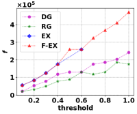
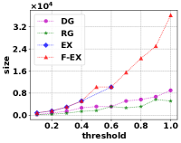
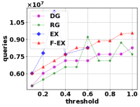
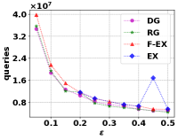
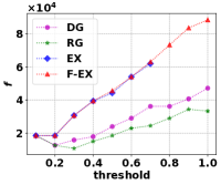
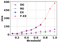
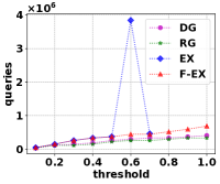
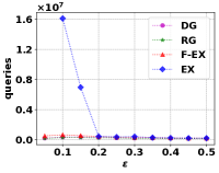
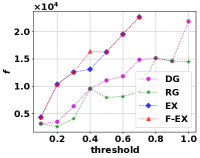
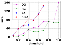
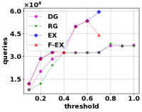
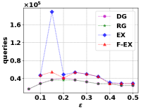
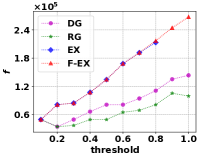
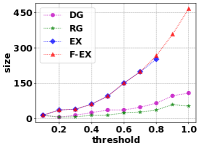
The results in terms of the $f$ values and size of the output solutions returned by the four algorithms are plotted in Figure 1(e) and Figure 1(f). From the plots, one can see that the $f$ values satisfy that $f(S_{\text{exact}})\approx f(S_{\text{f-exact}})>f(S_{\text{DG}})>f(S_{\text{RG}})$. This is due to the stopping conditions for each algorithm, which follow from each algorithms approximation guarantee on $f$ of $1-\epsilon$, $1-\epsilon$, 1/2, and $1/e$ respectively. On the other hand, the size mirrors the $f$ value, since it tends to be the case that reaching a higher $f$ value requires more elements from $U$. The number of queries made by the algorithms can be seen in Figure 1(h) and 1(g). As expected, the exact algorithms make more queries compared to the approximation algorithms, and in some cases "EX" doesn’t even finish. However, by taking advantage of the properties (i) and (ii) discussed above, "F-EX" is able to run even for smaller $\epsilon$. Therefore, depending on the application, an exact algorithm on the relatively small set $\cup S_{i}$ may be a practical choice in order to achieve a solution that is very close to feasible.

4 Appendix for Section 2

In this portion of the appendix, we present missing details and proofs from Section 2 in the main paper. We first present missing content from Section 2.1 in Section 4.1, followed by missing content from Section 2.2 in Section 4.2, and finally missing content from Section 2.3 is presented in Section 4.3. In this section, we include a more detailed comparison of the algorithms presented in this paper. In addition, pseudocode for the algorithm convert of Iyer and Bilmes [2013b] is presented in Algorithm 4.

Table 1: Theoretical guarantees of a subset of algorithms in this paper

Alg name	$f$ value	soln size	number of queries
greedy-c	$(1-\epsilon)\tau$	$\ln(1/\epsilon)$	$O(n\ln(1/\epsilon)|OPT|)$
stoch-greedy-c	$(1-\epsilon)\tau$	$(1+\alpha)\ln(3/\epsilon)$	$O(\frac{\alpha}{1+\alpha}n\ln(1/\delta)\ln^{2}(1/\epsilon)\ln(|OPT|))$
thresh-greedy-c	$(1-\epsilon)\tau$	$\ln(2/\epsilon)+1$	$O(\frac{n}{\epsilon}\ln(\frac{|OPT|}{\epsilon}))$
stream-c	$(1-\epsilon)\tau$	$(1+\alpha)(2/\epsilon+1)|OPT|$	$O(\log(|OPT|)(\frac{n}{\epsilon}+\mathcal{T}((1+\alpha)|OPT|/\epsilon^{2}))$

Algorithm 4 convert

Input: An SC instance with threshold $\tau$, a $(\gamma,\beta)$-bicriteria approximation algorithm for SMP, $\alpha>0$
Output: $S\subseteq U$

1:$\kappa\leftarrow(1+\alpha)$, $S\leftarrow\emptyset$.

2:while $f(S)<\gamma\tau$ do

3:     $S\leftarrow(\gamma,\beta)$-bicriteria approximation for SMP with budget $\kappa$

4:     $\kappa\leftarrow(1+\alpha)\kappa$

5:return $S$

4.1 Additional content to Section 2.1

In this section, we present the detailed statement and proofs of the randomized converting theorem convert-rand, and the proofs for the theoretical results of the thresh-greedy-c and stoch-greedy-c algorithms. The pseudocode for thresh-greedy-c is in Algorithm 5. We now provide a proof of Theorem 1.

Theorem 1. thresh-greedy-c produces a solution with $(\ln(2/\epsilon)+1,1-\epsilon)$-bicriteria approximation guarantee to MSCP, in $O(\frac{n}{\epsilon}\log(\frac{n}{\epsilon}))$ number of queries of $f$.

Proof.

Let $r_{0}$ be defined as $r_{0}=\ln(\frac{2}{\epsilon})|OPT|$. By Claim 3.1 in Badanidiyuru and Vondrák [2014], we have that any $s\in U$ that is added to $S$ on Line 6 of Algorithm 5 would satisfy

$$\Delta f(S,s)\geq\frac{1-\epsilon/2}{|OPT|}\sum_{u\in OPT/S}\Delta f(S,u)$$

when it was added. It follows by submodularity that

$$\Delta f(S,s)\geq\frac{1-\epsilon/2}{|OPT|}\sum_{u\in OPT/S}\Delta f(S,u)\geq\frac{1-\epsilon/2}{|OPT|}(f(OPT)-f(S)).$$

And by re-arranging the above equation, and using induction over the elements added to $S$, we have that

$$f(S)\geq\left(1-\left(1-\frac{1-\epsilon/2}{|OPT|}\right)^{i}\right)f(OPT).$$

Then at the $r_{0}$-th time of adding new element, it is the case that

$$f(S)\geq\left(1-\left(1-\frac{1-\epsilon/2}{|OPT|}\right)^{r_{0}}\right)f(OPT)\geq(1-\epsilon)f(OPT)\geq(1-\epsilon)\tau.$$

Thus the condition on Line 3 is satisfied by this point and the algorithm stops after adding the $r_{0}$-th element. The output solution set satisfies that $|S|\leq|r_{0}|$.

We now analyze the number of queries made to $f$. We claim that the algorithm stops before $w=\epsilon\max_{u\in U}f(u)/|OPT|$. This is because at the end of the iteration of the while loop in Algorithm 5 corresponding to $w=\epsilon\max_{u\in U}f(u)/|OPT|$, we have that $\Delta f(S,s)<w$ for any $s\in U\setminus S$. Therefore

$$\sum_{s\in OPT/S}\Delta f(S,s)<|OPT/S|w\leq\epsilon\max_{u\in U}f(u)\leq\epsilon f(OPT).$$

It follows that at the end of this iteration of the while loop that $f(S)>(1-\epsilon)f(OPT)$, which means the condition on Line 3 is not satisfied and the algorithm terminates. The number of iterations is thus $O\left(\frac{\ln(|OPT|/\epsilon)}{\epsilon}\right)$ and the query complexity is $O\left(\frac{n}{\epsilon}\ln\left(\frac{|OPT|}{\epsilon}\right)\right)$. ∎

Algorithm 5 thresh-greedy-c

Input: $\epsilon$
Output: $S\subseteq U$

1:$S\leftarrow\emptyset$

2:$w=\max_{u\in U}f(u)$

3:while $f(S)<(1-\epsilon)\tau$ do

4:     for  each $u$ in $U$ do

5:         if $\Delta f(S,u)\geq w$ then

6:              $S\leftarrow S\cup\{u\}$               

7:     $w=w(1-\frac{\epsilon}{2})$

8:return $S$

Next, we consider the algorithm convert-rand that converts algorithms for monotone SMP to ones for MSCP. Pseudocode for convert-rand is provided in Algorithm 6. We now present the proof of Theorem 2.

Algorithm 6 convert-rand

Input: A MSCP instance with threshold $\tau$, a $(1-\frac{\epsilon}{2},\beta)$-bicriteria approximation algorithm for monotone SMP where $\epsilon$ is in expectation, $\alpha>0$
Output: $S\subseteq U$

1:$S_{i}\leftarrow\emptyset$, $\forall i\in\{1,...,\ln(1/\delta)/\ln(2)\}$

2:$g\leftarrow(1+\alpha)$

3:while $f(S_{i})<(1-\epsilon))\tau$ $\forall i$ do

4:     for $i\in\{1,...,\ln(1/\delta)/\ln(2)\}$ do

5:         $S_{i}\leftarrow(1-\epsilon/2,\beta)$-bicriteria approximation for monotone SMP with objective function $f_{\tau}$ and budget $g$      

6:     $g\leftarrow(1+\alpha)g$

7:return $S$

Theorem 2. Any randomized $(1-\epsilon/2,\beta)$-bicriteria approximation algorithm for monotone SMP that runs in time $\mathcal{T}(n)$ where $\epsilon$ holds only in expectation can be converted into a $((1+\alpha)\beta,1-\epsilon)$-bicriteria approximation algorithm for MSCP that runs in time $O(\log_{1+\alpha}(|OPT|)\ln(1/\delta)\mathcal{T}(n))$ where $\epsilon$ holds with probability at least $1-\delta$.

Proof.

Consider the run of the algorithm for monotone SMP on Line 3 of Algorithm 6 when the parameter $g$ falls into the region $|OPT|\leq g\leq(1+\alpha)|OPT|$. Notice that it is the case that $f_{\tau}$ is also monotone and submodular. By the theoretical guarantees of the algorithm for monotone SMP, we have that for all $i\in\{1,...,\ln(1/\delta)/\ln(2)\}$

$$\mathbb{E}f_{\tau}(S_{i}) \geq(1-\epsilon/2)\max_{|X|\leq g}\{f_{\tau}(X)\}\geq(1-\epsilon/2)\max_{|X|\leq|OPT|}\{f_{\tau}(X)\}\geq(1-\epsilon/2)\tau.$$

From Markov’s inequality, we have that for each $i\in\{1,...,\ln(1/\delta)/\ln(2)\}$

$$P(f_{\tau}(S_{i})\leq(1-\epsilon)\tau)\leq P(\tau-f_{\tau}(S_{i})>2(\tau-\mathbb{E}f_{\tau}(S_{i})))\leq 1/2.$$

Then the probability that none of the subsets $S_{i}$ can reach the stopping condition can be bounded by

$$P(f(S_{i})\leq(1-\epsilon)\tau,\forall i) =P(f_{\tau}(S_{i})\leq(1-\epsilon)\tau,\forall i)$$

$$=\prod_{i=1}^{\ln(1/\delta)/\ln(2)}P(f_{\tau}(S_{i})\leq(1-\epsilon)\tau)$$

$$\leq(1/2)^{\ln(1/\delta)/\ln(2)}=\delta.$$

This means with probability at least $1-\delta$, convert-rand stops when $g$ reaches the region where $|OPT|\leq g\leq(1+\alpha)|OPT|$ since the condition of the while loop is not satisfied.

∎

Before we present the proof of the theoretical guarantees of the algorithm stoch-greedy-c, we first introduce an algorithm for monotone SMP with bicriteria approximation guarantee called stoch-bi. stoch-bi is an extension of the stochastic greedy algorithm of Mirzasoleiman et al. [2015a], which produces an infeasible solution to the instance of monotone SMP that has $f$ value arbitrarily close to that of the optimal solution. Pseudocode for stoch-bi is provided in Algorithm 7. Notice that if we use the stoch-bi as a subroutine for convert-rand, we can obtain an algorithm for MSCP that runs in $O(n\ln^{2}(3/\epsilon)\ln(1/\delta)\log_{1+\alpha}|OPT|)$, which is less queries than the standard greedy algorithm, but worse than our algorithm stoch-greedy-c by a factor of $(1+\alpha)/\alpha$.

Algorithm 7 stoch-bi

Input: $\epsilon>0$
Output: $S\subseteq U$

1:$S\leftarrow\emptyset$

2:while $|S|<\ln(\frac{3}{2\epsilon})\kappa$ do

3:     $R\leftarrow$ sample $\frac{n}{\kappa}\ln(\frac{3}{2\epsilon})$ elements from $U$

4:     $u\leftarrow\text{argmax}_{x\in R}\Delta f(S,x)$

5:return $S$

Theorem 7.

stoch-bi produces a solution with $(1-\epsilon,\ln(\frac{3}{2\epsilon}))$-bicriteria approximation guarantee to MSMP, where the $1-\epsilon$ holds in expectation, in $O(n\ln^{2}(\frac{3}{2\epsilon}))$ queries of $f$.

Proof.

Our argument to prove Theorem 7 follows a similar approach as Mirzasoleiman et al. [2015a]. Let the partial solution $S$ before $i$-th iteration of the while loop of Algorithm 7 be $S_{i}$, the item that is added to set $S$ during iteration $i$ be $u_{i}$, and the sampled set $R$ during iteration $i$ be $R_{i}$. Consider the beginning of any iteration $i$ of the while loop. Then because of the greedy choice for $u_{i}$ it is the case that if $R_{i}\cap OPT\neq\emptyset$,

$$\Delta f(S_{i},u_{i})\geq\Delta f(S_{i},x)$$

for all $x\in R_{i}\cap OPT$. Therefore we have that in expectation over the randomly chosen set $R_{i}$

$$\mathbb{E}[\Delta f(S_{i},u_{i})|S_{i}] \geq\textbf{Pr}(R_{i}\cap OPT\neq\emptyset)\mathbb{E}[\Delta f(S_{i},u_{i})|S_{i},R_{i}\cap OPT\neq\emptyset]$$

$$\geq\textbf{Pr}(R_{i}\cap OPT\neq\emptyset)\frac{1}{|R_{i}\cap OPT|}\sum_{x\in R_{i}\cap OPT}\Delta f(S_{i},x)$$

$$=\textbf{Pr}(R_{i}\cap OPT\neq\emptyset)\frac{1}{\kappa}\sum_{x\in OPT}\Delta f(S_{i},x)$$ (1)

where the last inequality follows since the elements of $R_{i}$ are chosen uniformly randomly, implying that all elements of $OPT$ are equally likely to be chosen.

Let the number of samples $s=\frac{n}{k}\ln(\frac{3}{2\epsilon})$. The probability $\textbf{Pr}(R_{i}\cap OPT\neq\emptyset)$ can be lower bounded as

$$\textbf{Pr}(R_{i}\cap OPT\neq\emptyset) =1-\textbf{Pr}(R_{i}\cap OPT=\emptyset)$$

$$=1-\frac{\binom{n-\kappa}{s}}{\binom{n}{s}}$$

$$\geq 1-(\frac{n-\kappa}{n})^{s}$$

$$\geq 1-\frac{2\epsilon}{3},$$ (2)

where the last inequality comes from the fact that $(1-\frac{1}{x})^{x}\leq e^{-1}$. By submodularity, we have

$$\sum_{u\in OPT}\Delta f(S_{i},u)\geq f(OPT)-f(S_{i}).$$ (3)

Plug Equations (4.1) and (3) into (4.1) yields that

$$\mathbb{E}[\Delta f(S_{i},u_{i})|S_{i}]\geq\frac{1-2\epsilon/3}{\kappa}(f(OPT)-f(S_{i})).$$ (4)

Therefore,

$$\mathbb{E}[f(S_{i+1})|S_{i}]\geq\frac{1-2\epsilon/3}{\kappa}f(OPT)+(1-\frac{1-2\epsilon/3}{\kappa})f(S_{i})).$$

By induction and by taking expectation over $S_{i}$, we can get that at the last iteration

$$\mathbb{E}[f(S)] \geq\frac{1-2\epsilon/3}{\kappa}\sum_{i=0}^{|S|-1}(1-\frac{1-2\epsilon/3}{\kappa})^{i}f(OPT)$$

$$\geq\{1-(1-\frac{1-2\epsilon/3}{\kappa})^{|S|}\}f(OPT)$$

$$\geq(1-(2\epsilon/3)^{1-2\epsilon/3})f(OPT)\geq(1-\epsilon)f(OPT),$$

where in the last inequality, we use the fact that $|S|=\ln(3/2\epsilon)\kappa$. ∎

We now present the omitted proofs for Lemmas 1, 2, and 3 about our algorithm stoch-greedy-c. Once these lemmas are proven, we next prove Theorem 3 using the lemmas.

Lemma 1. Define $\ell$ to be the integer such that $(1+\alpha)^{\ell-1}\leq|OPT|\leq(1+\alpha)^{\ell}$. Consider any of the sets $S_{i}$ at the beginning of an iteration on Line 4 where $g\leq(1+\alpha)^{\ell}$. Then if $u_{i}$ is the random element that will be added on Line 6, we have that

$$\mathbb{E}[\Delta f_{\tau}(S_{i},u_{i})|S_{i}]\geq\frac{1-\epsilon/3}{(1+\alpha)^{\ell}}(\tau-f_{\tau}(S_{i}))\geq\frac{1-\epsilon/3}{(1+\alpha)|OPT|}(\tau-f_{\tau}(S_{i})).$$

Proof.

Define $OPT^{*}=\arg\max_{|X|\leq(1+\alpha)^{\ell}}f(X).$ Then we have $f(OPT^{*})\geq f(OPT)\geq\tau$. Therefore $f_{\tau}(OPT^{*})\geq\tau$. Consider an iteration of the while loop on Line 4 of stoch-greedy-c where $g\leq(1+\alpha)^{\ell}$, and some iteration of inside for loop corresponding to set $S_{i}$. From Line 5 of stoch-greedy-c, we have that the size of the randomly sampled subset $R_{i}$ for $S_{i}$ is $\min\{n,n\ln(3/\epsilon)/g\}$. Then if $n\ln(3/\epsilon)/g<n$, we have that

$$|R_{i}|=\frac{n}{g}\ln(3/\epsilon)\geq\frac{n}{(1+\alpha)^{\ell}}\ln(3/\epsilon).$$

This implies that if $n\ln(3/\epsilon)/g<n$, when we randomly sample $R_{i}$

$$P(R_{i}\cap OPT^{*}=\emptyset)=(1-|OPT^{*}|/n)^{|R_{i}|}\leq(1-(1+\alpha)^{\ell}/n)^{\frac{n\ln(3/\epsilon)}{(1+\alpha)^{\ell}}}\leq\epsilon/3.$$

On the other hand, if $n\ln(3/\epsilon)/g\geq n$, then $P(R_{i}\cap OPT^{*}=\emptyset)=0$ and the above inequality also holds.

Notice that $f_{\tau}$ is monotone and submodular. Let $u_{i}$ be the elements of $R_{i}$ which will be added to $S_{i}$. Then

$$\mathbb{E}[\Delta f_{\tau}(S_{i},u_{i})|R_{i}\cap OPT^{*}\neq\emptyset] \geq\frac{1}{|OPT^{*}|}\sum_{o\in OPT^{*}}\Delta f_{\tau}(S_{i},o)$$

$$\stackrel{{\scriptstyle\mathclap{\mbox{(i)}}}}{{\geq}}\frac{1}{|OPT^{*}|}(f_{\tau}(OPT^{*})-f_{\tau}(S_{i}))$$

$$\geq\frac{1}{(1+\alpha)^{\ell}}(\tau-f_{\tau}(S_{i})).$$

where (i) is implied by the fact that $f_{\tau}$ is monotone and submodular. Altogether we have that

$$\mathbb{E}[\Delta f_{\tau}(S_{i},u_{i})|S_{i}] \geq P(R\cap OPT^{*}\neq\emptyset)\mathbb{E}[\Delta f_{\tau}(S_{i},u_{i})|R\cap OPT^{*}\neq\emptyset]$$

$$\geq\frac{1-\epsilon/3}{(1+\alpha)^{\ell}}(\tau-f_{\tau}(S_{i})).$$

∎

Lemma 2. Once $r\geq(1+\alpha)\ln(3/\epsilon)|OPT|$, we have that $\mathbb{E}[f_{\tau}(S_{i})]\geq\left(1-\frac{\epsilon}{2}\right)\tau$ for all $i$.

Proof.

Define $\ell$ to be the integer such that $(1+\alpha)^{\ell-1}\leq|OPT|\leq(1+\alpha)^{\ell}$. Then notice that throughout stoch-greedy-c until $r$ is incremented to be $\ln(3/\epsilon)(1+\alpha)^{\ell}$, it is the case that $g\leq(1+\alpha)^{\ell}$. Therefore Lemma 1 applies for all marginal gains of adding elements to the sets until the end of the $\ln(3/\epsilon)(1+\alpha)^{\ell}$ iteration of the while loop. Consider any of the sets $S_{i}$. By applying recursion to Lemma 1, we have that at the end of any iteration $r\leq\ln(3/\epsilon)(1+\alpha)^{\ell}$ of the while loop

$$\mathbb{E}[f_{\tau}(S_{i})]\geq\left(1-\left(\frac{1-\epsilon/3}{(1+\alpha)^{\ell}}\right)^{r}\right)\tau.$$

Therefore, Once $r$ reaches $\ln(3/\epsilon)(1+\alpha)^{\ell}$, the expectation of $S_{i}$ is

$$\mathbb{E}[f_{\tau}(S_{i})]\geq\left(1-\left(\frac{1-\epsilon/3}{(1+\alpha)^{\ell}}\right)^{(1+\alpha)^{\ell}\ln(3/\epsilon)}\right)\tau\geq\left(1-\frac{\epsilon}{2}\right)\tau.$$

Because $\ln(3/\epsilon)(1+\alpha)^{\ell}\leq(1+\alpha)\ln(3/\epsilon)|OPT|$ and $f$ is monotonic, Lemma 2 holds. ∎

Lemma 3. With probability at least $1-\delta$, once $r\geq(1+\alpha)\ln(3/\epsilon)|OPT|$, we have that $\max_{i}f(S_{i})\geq(1-\epsilon)\tau$.

Proof.

Since $f_{\tau}(S)=\min\{f(S),\tau\}$, we have that $\tau-f_{\tau}(S)\in[0,\tau]$ for any $S\in U$. By applying the Markov’s inequality, we have that

$$P(\tau-f_{\tau}(S_{j})\geq 2\mathbb{E}(\tau-f_{\tau}(S_{j}))\leq\frac{1}{2}$$

From Lemma 2, we have $\mathbb{E}(\tau-f_{\tau}(S_{j}))\leq\frac{\epsilon\tau}{2}$. Then

$$P(f_{\tau}(S_{j})\leq(1-\epsilon)\tau) =P(\tau-f_{\tau}(S_{j})\geq\epsilon\tau)$$

$$\leq P(\tau-f_{\tau}(S_{j})\geq 2\mathbb{E}(\tau-f_{\tau}(S_{j})))$$

$$\leq\frac{1}{2}.$$

Thus we have

$$P(\max_{j}f_{\tau}(S_{j})>(1-\epsilon)\tau) =1-P(f_{\tau}(S_{j})\leq(1-\epsilon)\tau,\forall j)$$

$$=1-P(f_{\tau}(S_{1})\leq(1-\epsilon)\tau)^{\ln(1/\delta)/\ln(2)}$$

$$\geq 1-\left(\frac{1}{2}\right)^{\ln(1/\delta)/\ln(2)}\geq 1-\delta.$$

∎

Theorem 3. Suppose that stoch-greedy-c is run for an instance of MSCP. Then with probability at least $1-\delta$, stoch-greedy-c outputs a solution $S$ that satisfies a $((1+\alpha)\ln(3/\epsilon),1-\epsilon)$-bicriteria approximation guarantee in at most

$$O\left(\frac{\alpha}{1+\alpha}n\ln(1/\delta)\ln^{2}(3/\epsilon)\log_{1+\alpha}(|OPT|)\right)$$

queries of $f$.

Proof.

From Lemma 3, we have that the algorithm stops by the time $r$ reaches $(1+\alpha)\ln(3/\epsilon)|OPT|$ with probability at least $1-\delta$. Before $r$ reaches this point, consider the number of queries made to $f$ over the duration that $g$ is a certain value $(1+\alpha)^{m}$. Then for each of the $O(\ln(1/\delta))$ sets a total of at most

$$\left(\ln\left(\frac{3}{\epsilon}\right)(1+\alpha)^{m}-\ln\left(\frac{3}{\epsilon}\right)(1+\alpha)^{m-1}\right)\frac{n\ln(\frac{3}{\epsilon})}{(1+\alpha)^{m}}=\frac{\alpha}{1+\alpha}n\ln^{2}(3/\epsilon)$$

queries are made to $f$. Because $g$ takes on at most $O(\log_{1+\alpha}(|OPT|))$ values before $r$ reaches $(1+\alpha)\ln(3/\epsilon)|OPT|$, Theorem 3 follows. ∎

4.2 Additional content for Section 2.2

In this section, we present the proofs of theoretical results from Section 2.2. First, in Claim 1 we present a useful claim from Crawford [2023] about submodular functions in order to prove Lemma 4. Next, we use Claim 1 in order to prove Lemma 4. Finally, Lemma 4 is used to prove the main result for stream-c, Theorem 4.

Claim 1 (Claim 1 in Crawford [2023]).

Let $A_{1},...,A_{m}\subseteq U$ be disjoint, and $B\subseteq U$. Then there exists $i\in\{1,...,m\}$ such that $f(A_{i}\cup B)\geq(1-1/m)f(B)$.

Lemma 4. By the time that $g$ reaches the region $[|OPT|,(1+\alpha)|OPT|]$ and the loop on Line 4 of stream-c has completed, there exists a set $X\subseteq\cup S_{i}$ of size at most $(2/\epsilon+1)g$ such that $f(X)\geq(1-\epsilon)\tau$.

Proof.

Suppose that stream-c has reach the end of the loop on Line 4 when $g\geq|OPT|$. We first consider the case where there exists some set $S_{t}$ $t\in\{1,...,2/\epsilon\}$ such that $|S_{t}|=2g/\epsilon$. In this case it follows that $f(S_{t})=\sum_{i=1}^{2g/\epsilon}\Delta f(S_{t}^{i},u_{i})\geq\tau$, where $S_{t}^{i}$ is the set of $S_{t}$ before adding the $i$-th element $u_{i}$, and so the Lemma statement is proven.

Next, we consider the case where $|S_{j}|<2g/\epsilon$, $\forall j\in[2/\epsilon]$. Let $OPT_{1}=OPT\cap(\cup_{i=1}^{2/\epsilon}S_{i})$ and $OPT_{2}=OPT/OPT_{1}$. By Claim 1, there exists a set $S_{t}$ such that

$$f(S_{t}\cup OPT)\geq(1-\epsilon/2)f(OPT)\geq(1-\epsilon/2)\tau.$$

Since $|S_{t}|<2g/\epsilon$ at the end of the algorithm, we can see each element $o$ in $OPT_{2}$ is not added into $S_{t}$ because $\Delta f(S_{t},o)\leq\epsilon\tau/(2g)$ at the time $o$ is seen in the loop on Line 4. By submodularity and the fact that $g\geq|OPT|\geq|OPT_{2}|$,

$$\sum_{o\in OPT_{2}}\Delta f(S_{t}\cup OPT_{1},o)<\epsilon|OPT_{2}|\tau/(2g)\leq\epsilon\tau/2.$$

Therefore

$$(1-\epsilon/2)\tau \leq f(S_{t}\cup OPT)$$

$$\leq f(S_{t}\cup OPT_{1})+\Delta f(S_{t}\cup OPT_{1},OPT_{2})$$

$$\leq f(S_{t}\cup OPT_{1})+\sum_{o\in OPT_{2}}\Delta f(S_{t}\cup OPT_{1},o)$$

$$\leq f(S_{t}\cup OPT_{1})+\epsilon\tau/2.$$

Therefore $f(S_{t}\cup OPT_{1})\geq(1-\epsilon)\tau$. Because $S_{t}\cup OPT_{1}\subseteq\cup S_{i}$, and it is the case that $|S_{t}\cup OPT_{1}|\leq|S_{t}|+|OPT_{1}|\leq 2g/\epsilon+g$, so the Lemma statement is proven. ∎

Theorem 4. Suppose that stream-c is run for an instance of SCP. Then stream-c returns $S$ such that $f(S)\geq(1-\epsilon)\tau$ and $|S|\leq(1+\alpha)(2/\epsilon+1)|OPT|$ in at most

$$\log_{1+\alpha}(|OPT|)\left(\frac{2n}{\epsilon}+\mathcal{T}\left((1+\alpha)\left(\frac{4}{\epsilon^{2}}|OPT|\right)\right)\right)$$

queries of $f$, where $\mathcal{T}(m)$ is the number of queries to $f$ of the algorithm for SMP used on Line 7 of Algorithm 2 on an input set of size $m$.

Proof.

By Lemma 4, once stream-c reaches $g\geq|OPT|$ then $f(S)\geq(1-\epsilon)\tau$ will be satisfied and therefore the while loop will exit. This implies that $g\leq(1+\alpha)|OPT|$ once stream-c exits, and therefore $|S|\leq(2/\epsilon+1)g\leq(1+\alpha)(2/\epsilon+1)|OPT|$. Therefore the qualities of $S$ stated in Theorem 4 are proven. As far as the number of queries of $f$, it takes at most $\log_{1+\alpha}(|OPT|)$ iterations of the loop to reach the point that $g\geq|OPT|$. In addition, each iteration of the loop makes $\frac{2n}{\epsilon}+\mathcal{T}\left((1+\alpha)\left(\frac{4}{\epsilon^{2}}|OPT|\right)\right)$ queries of $f$. Therefore the bound on the number of queries of $f$ in Theorem 4 is proven. ∎

4.3 Supplementary material to Section 2.3

We now present additional theoretical details for Section 2.3, where we considered regularized SCP. First, we prove Theorem 5 about our algorithm convert-reg which converts algorithms for regularized SMP into ones for RSCP.

Theorem 5. Suppose that we have an algorithm reg for maximization of a regularized submodular function subject to a cardinality constraint $\kappa$, and that algorithm is guaranteed to return a set $S$ of cardinality at most $\rho\kappa$ such that

$$g(S)-c(S)\geq\gamma g(X)-\beta c(X)$$

for all $X$ such that $|X|\leq\kappa$ in time $T(n)$. Then the algorithm convert-reg using reg as a subroutine returns a set $S$ such that

$$g(S)-\frac{\gamma}{\beta}c(S)\geq\gamma\tau$$

and $|S|\leq(1+\alpha)\rho|OPT|$ in time $O(\log_{1+\alpha}(n)T(n))$.

Proof.

Let $OPT$ be the optimal solution to the instance of regularized SCP. Consider the iteration of convert-reg where $\kappa$ has just increased above $|OPT|$, i..e $|OPT|\leq\kappa\leq(1+\alpha)|OPT|$. Then we run reg with input objective $g-\frac{\gamma}{\beta}c$ and budget $\kappa\geq|OPT|$. Then by the assumptions on reg we have that

$$g(S)-\frac{\gamma}{\beta}c(S)\geq\gamma(g(OPT)-c(OPT))\geq\gamma\tau$$

and $|S|\leq\rho\kappa\leq(1+\alpha)\rho|OPT|$. ∎

We now fill in the missing information concerning our algorithm distorted-bi. Recall the definition of

$$\Phi_{i}(X)=\left(1-\frac{1}{\kappa}\right)^{t-i}g(X)-c(X),$$

where $t=\ln(1/\epsilon)\kappa$, which is used in both the pseudocode for distorted-bi and throughout the proofs. First, pseudocode for distorted-bi is presented in Algorithm 8. Next, we present and prove Lemma 5, and then use Lemma 5 in order to prove our main result for distorted-bi, Theorem 6.

Lemma 5.

Consider any iteration $i+1$ of the while loop in distorted-bi. Let $S_{i}$ be defined to be $S$ after the $i$-th iteration of the while loop in distorted-bi. Then for any $X\subseteq U$ such that $|X|\leq\kappa$,

$$\Phi_{i+1}(S_{i+1})-\Phi_{i}(S_{i})\geq\frac{1}{\kappa}\left(1-\frac{1}{\kappa}\right)^{t-(i+1)}g(X)-\frac{c(X)}{\kappa}.$$

Proof.

First, suppose that during iteration $i+1$ an element $s_{i+1}$ was added to $S$. First, notice that

$$\Phi_{i+1}(S_{i+1})-\Phi_{i}(S_{i}) =\Phi_{i+1}(S_{i+1})-\Phi_{i+1}(S_{i})+\Phi_{i+1}(S_{i})-\Phi_{i}(S_{i})$$

$$=\Delta\Phi_{i+1}(S_{i},s_{i+1})+\frac{1}{\kappa}\left(1-\frac{1}{\kappa}\right)^{t-(i+1)}g(S_{i}).$$ (5)

In addition, notice that for any subset of $U$ such that $|X|\leq\kappa$

$$\Delta\Phi_{i+1}(S_{i},s_{i+1}) \overset{(a)}{\geq}\frac{1}{\kappa}\sum_{o\in X}\left(\Delta\Phi_{i+1}(S_{i},o)\right)$$

$$\geq\frac{1}{\kappa}\sum_{o\in X}\left(\left(1-\frac{1}{\kappa}\right)^{t-(i+1)}\Delta g(S_{i},o)-\Delta c(S_{i},o)\right)$$

$$\geq\frac{1}{\kappa}\left(1-\frac{1}{\kappa}\right)^{t-(i+1)}\sum_{o\in X}\Delta g(S_{i},o)-\frac{c(X)}{\kappa}$$

$$\overset{(b)}{\geq}\frac{1}{\kappa}\left(1-\frac{1}{\kappa}\right)^{t-(i+1)}\left(g(S_{i}\cup X)-g(S_{i})\right)-\frac{c(X)}{\kappa}$$

$$\overset{(c)}{\geq}\frac{1}{\kappa}\left(1-\frac{1}{\kappa}\right)^{t-(i+1)}\left(g(X)-g(S_{i})\right)-\frac{c(X)}{\kappa}$$

where (a) is because of the greedy choice of $s_{i}$; (b) is by the submodularity of $g$; and (c) is by the monotonicity of $g$. Combining the previous two equations gives the result of Lemma 5.

Next, we consider the case where $\Delta\Phi_{i}(S_{i},x)\leq 0$ for all $x\in U$, and so there is no new element added. In this case, we can randomly choose an element from the current solution $S_{i}$ as the added element $s_{i+1}$. It is not hard to verify that the above two inequalities still holds in this case, and therefore again we have the result of Lemma 5. ∎

Algorithm 8 distorted-bi

Input: $\epsilon$
Output: $S\subseteq U$

1:$S\leftarrow\emptyset$

2:$i\leftarrow 1$

3:while $|S|<\ln(1/\epsilon)\kappa$ do

4:     $u\leftarrow\text{argmax}_{x\in U}\Delta\Phi_{i}(S,x)$

5:     if $\Delta\Phi_{i}(S,x)>0$ then

6:         $S\leftarrow S\cup\{u\}$

7:         $i\leftarrow i+1$

8:     else

9:         break      

10:return $S$

Theorem 6. Suppose that distorted-bi is run for an instance of regularized SMP. Then distorted-bi produces a solution $S$ in $O(n\kappa\ln(1/\epsilon))$ queries of $f$ such that $|S|\leq\ln(1/\epsilon)\kappa$ and for all $X\subseteq U$ such that $|X|\leq\kappa$, $g(S)-c(S)\geq(1-\epsilon)g(X)-\ln(1/\epsilon)c(X).$

Proof.

We will use Lemma 5 to prove Theorem 6. Define $t=\ln(1/\epsilon)\kappa$. Then we see that

$$g(S_{t})-c(S_{t}) \overset{(a)}{\geq}\Phi_{t}(S_{t})-\Phi_{0}(S_{0})$$

$$=\sum_{i=0}^{t-1}\left(\Phi_{i+1}(S_{i+1})-\Phi_{i}(S_{i})\right)$$

$$\overset{(b)}{\geq}\sum_{i=0}^{t-1}\left(\frac{1}{\kappa}\left(1-\frac{1}{\kappa}\right)^{t-(i+1)}g(X)-\frac{c(X)}{\kappa}\right)$$

$$=\frac{g(X)}{\kappa}\sum_{i=0}^{t-1}\left(1-\frac{1}{\kappa}\right)^{t-(i+1)}-\ln\left(1/\epsilon\right)c(X)$$

$$=\frac{g(X)}{\kappa}\sum_{i=0}^{t-1}\left(1-\frac{1}{\kappa}\right)^{i}-\ln\left(1/\epsilon\right)c(X)$$

$$\overset{(c)}{=}\left(1-\left(1-\frac{1}{\kappa}\right)^{t}\right)g(X)-\ln\left(1/\epsilon\right)c(X)$$

$$\geq(1-\epsilon)g(X)-\ln\left(1/\epsilon\right)c(X)$$

where (a) is because $g(\emptyset)\geq 0$; (b) is because Lemma 5; and (c) is by the formula for geometric series. ∎

5 Supplementary material for Section 3

In this section, we present supplementary material to Section 3. In particular, we present additional detail about the experimental setup in Section 5.1, and additional experimental results in Section 5.2.

5.1 Experimental setup

First of all, we provide more detail about the two applications used to evaluate the algorithms proposed in the main paper. For monotone SCP, the application considered here is data summarization, where $f$ is a function that represents how well a subset could summarize the whole dataset. The problem definition is as follows.

Definition 1.

(Data Summarization) Suppose there are a total of $n$ elements denoted as $U$. Let $T$ be a set of tags. Each element in $U$ is tagged with a set of elements from $T$ via function $t:U\rightarrow 2^{T}$. The function $f$ is defined as

$$f(S)=|\cup_{s\in S}t(s)|,\qquad\forall S\in U.$$

From the definition, we can see that $f$ is both monotone and submodular. For general SCP, the application we consider is where $f$ is a graph cut function, which is a submodular but not necessarily monotone function.

Definition 2.

(Graph cut) Let $G=(V,E)$ be a graph, and $w:E\rightarrow\mathbb{R}_{\geq 0}$ be a function that assigns a weight for evry edge in the graph. The function $f:2^{U}\rightarrow\mathbb{R}_{\geq 0}$ maps a subset of vertices $X\subseteq V$ to the total weight of edges between $X$ and $V\backslash X$. More specifically,

$$f(S)=\sum_{x\in X,y\in V\backslash X}w(x,y).$$

In addition to the datasets considered in the main paper, we also look at graph cut instances on the com-Amazon ($n=334863$, 925872 edges), ego-Facebook ($n=4039$, 88234 edges), and email-Enron ($n=36692$, 183831 edges) graphs from the SNAP large network collection [Leskovec and Sosič, 2016].

We now present more detail about the algorithms “EX” and “F-EX”. EX begins by using a greedy algorithm to find a solution that meets the desired threshold. If this greedy choice fails, EX begins a search of all feasible sets where each element considered is in order of decreasing marginal gains. Lazy updates are used for computing marginal gains. “F-EX” uses a similar approach as EX, but as described in the main paper limits the search to a smaller portion of the elements. In particular, as described in the main paper, the F-EX algorithm first checks if the optimization problem in line 7 of stream-c is an unconstrained SMP. If so, the algorithm adds all monotone elements from the the union of $\{S_{1},...S_{2/\epsilon}\}$ to the solution set and then explores the non-monotone elements in the rest of $\cup_{i=1}^{2/\epsilon}S_{i}$.

5.2 Additional experimental results

First of all, we present some additional monotone experimental results on the synthetic data and the corel dataset. The corel dataset is the Corel5k set of images in Duygulu et al. [2002] ($n=4500$). The synthetic data we used here is a data summarization instance with a total of $m=4000$ elements and 2000 ($n=2000$) subset of elements. Each subset is randomly generated in the following way: let us denote the set of elements as $[m]=\{1,2,3...,m\}$, each elements $i\leq 250$ is added to the subset with probability $0.4$, and each element $250<i\leq m$ is added with probability $0.002$. The four algorithms examined here can be found in Section 3. We compare the four algorithms for different value of $\tau$ and $\epsilon$. When $\epsilon$ is varied, $\tau$ is fixed at $0.9f(U)$ for corel dataset and synthetic dataset with $U$ being the universe of the two instances respectively. When $\tau$ is varied, $\epsilon$ is fixed at $0.05$. The results on the synthetic data are presented in Figure 2(a), 2(b), 2(c), and 2(d). The results on the corel dataset are plotted in Figure 2(e), 2(f), 2(g) and 2(h).From the results, we can see that the results on the corel dataset is in line with the results in the main paper. However, on the synthetic dataset, it is worth noting that the "SG" (stoch-greedy-c) algorithm requires less number of queries compared with other three algorithms even when $\epsilon$ is large, which further demonstrates the advantages of our algorithms.

(a) synthetic $f$

(b) synthetic $c$

(c) synthetic queries

(d) synthetic queries

(e) corel $f$

(f) corel $c$

(g) corel queries

(h) corel queries

Figure 2: The experimental results of running different greedy algorithms on the instances of data summarization on the synthetic dataset, and corel dataset.

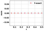
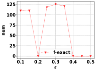
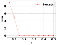
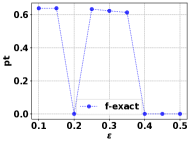
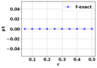
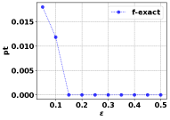
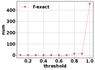
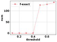
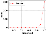
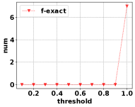
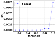
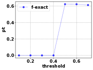
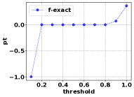
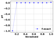
The additional experiments we present are further exploration of our algorithm stream-c. In Figure 3, we present additional experimental results analogous to those presented in the main paper for graph cut, but on the additional datasets described above. In summary, we see many of the same patterns exhibited on these instances as discussed in the main paper. In addition, we include an additional set of experiments analyzing how many non-monotone elements there are in the union of $\{S_{1},...S_{2/\epsilon}\}$ in stream-c in order to analyze how effective we would expect F-EX to be. The number (“num”) and portion (“pt”) of the nonmonotone elements the union of $\{S_{1},...S_{2/\epsilon}\}$ on the instances with the graph cut objective are plotted in Figures 4 and 5. If that instance did not require an exact search (meaning that the initial greedy heuristic found a solution), then -1 is plotted. From the figures, we can see that in most cases, the number of nonmonotone elements is either $0$ or very small, which explains why the fast exact algorithm requires less queries than the exact algorithm in these cases. This implies that in many instances of SCP, stream-c is able to cut down the original instance to one that is nearly monotone and much easier to solve.

(a) amazon $f$

(b) amazon $c$

(c) amazon queries

(d) amazon queries

(e) enron $f$

(f) enron $c$

(g) enron queries

(h) enron queries

(i) facebook $f$

(j) facebook $c$

(k) facebook queries

(l) facebook queries

Figure 3: The experimental results of running stream-c on the instances of graph cut on the com-Amazon graph ("amazon"), email-Enron ("enron") and ego-Facebook ("facebook") dataset.

(a) amazon, $\tau=0.5\cdot f_{\text{ave-max}}$

(b) facebook, $\tau=0.5\cdot f_{\text{ave-max}}$

(c) enron, $\tau=0.7\cdot f_{\text{ave-max}}$

(d) euall, $\tau=0.9\cdot f_{\text{ave-max}}$

(e) amazon, $\tau=0.5\cdot f_{\text{ave-max}}$

(f) facebook, $\tau=0.5\cdot f_{\text{ave-max}}$

(g) enron, $\tau=0.7\cdot f_{\text{ave-max}}$

(h) euall, $\tau=0.9\cdot f_{\text{ave-max}}$

Figure 4: The second experiments. We plot the number and portion of the non-monotone elements. Here $x$-axis refers to value of $\tau$.

(a) amazon, $\epsilon=0.3$

(b) facebook, $\epsilon=0.3$

(c) enron, $\epsilon=0.2$

(d) euall, $\epsilon=0.15$

(e) amazon, $\epsilon=0.3$

(f) facebook, $\epsilon=0.3$

(g) enron, $\epsilon=0.2$

(h) euall, $\epsilon=0.15$

Figure 5: The second experiments. We plot the number and portion of the non-monotone elements. Here $x$-axis refers to value of $\epsilon$.

References

- Balkanski et al. [2018] Eric Balkanski, Adam Breuer, and Yaron Singer. Non-monotone submodular maximization in exponentially fewer iterations. Advances in Neural Information Processing Systems, 31, 2018.
- Iyer et al. [2021] Rishabh Iyer, Ninad Khargonkar, Jeff Bilmes, and Himanshu Asnani. Generalized submodular information measures: Theoretical properties, examples, optimization algorithms, and applications. IEEE Transactions on Information Theory, 68(2):752–781, 2021.
- Gillenwater et al. [2012] Jennifer Gillenwater, Alex Kulesza, and Ben Taskar. Near-optimal map inference for determinantal point processes. Advances in Neural Information Processing Systems, 25, 2012.
- Bateni et al. [2017] MohammadHossein Bateni, Hossein Esfandiari, and Vahab Mirrokni. Almost optimal streaming algorithms for coverage problems. In Proceedings of the 29th ACM Symposium on Parallelism in Algorithms and Architectures, pages 13–23, 2017.
- Kothawade et al. [2021] Suraj Kothawade, Nathan Beck, Krishnateja Killamsetty, and Rishabh Iyer. Similar: Submodular information measures based active learning in realistic scenarios. Advances in Neural Information Processing Systems, 34:18685–18697, 2021.
- Kothawade et al. [2022] Suraj Kothawade, Saikat Ghosh, Sumit Shekhar, Yu Xiang, and Rishabh Iyer. Talisman: targeted active learning for object detection with rare classes and slices using submodular mutual information. In Computer Vision–ECCV 2022: 17th European Conference, Tel Aviv, Israel, October 23–27, 2022, Proceedings, Part XXXVIII, pages 1–16. Springer, 2022.
- Bao et al. [2022] Wei-Xuan Bao, Jun-Yi Hang, and Min-Ling Zhang. Submodular feature selection for partial label learning. In Proceedings of the 28th ACM SIGKDD Conference on Knowledge Discovery and Data Mining, pages 26–34, 2022.
- El Halabi et al. [2022] Marwa El Halabi, Suraj Srinivas, and Simon Lacoste-Julien. Data-efficient structured pruning via submodular optimization. Advances in Neural Information Processing Systems, 35:36613–36626, 2022.
- Tschiatschek et al. [2014] Sebastian Tschiatschek, Rishabh K Iyer, Haochen Wei, and Jeff A Bilmes. Learning mixtures of submodular functions for image collection summarization. Advances in neural information processing systems, 27, 2014.
- Balakrishnan et al. [2022] Ravikumar Balakrishnan, Tian Li, Tianyi Zhou, Nageen Himayat, Virginia Smith, and Jeff Bilmes. Diverse client selection for federated learning via submodular maximization. In International Conference on Learning Representations, 2022.
- Nemhauser et al. [1978a] George L Nemhauser, Laurence A Wolsey, and Marshall L Fisher. An analysis of approximations for maximizing submodular set functions—i. Mathematical programming, 14(1):265–294, 1978a.
- Mirzasoleiman et al. [2015a] Baharan Mirzasoleiman, Ashwinkumar Badanidiyuru, Amin Karbasi, Jan Vondrák, and Andreas Krause. Lazier than lazy greedy. In Proceedings of the AAAI Conference on Artificial Intelligence, volume 29, 2015a.
- Harshaw et al. [2019] Chris Harshaw, Moran Feldman, Justin Ward, and Amin Karbasi. Submodular maximization beyond non-negativity: Guarantees, fast algorithms, and applications. In International Conference on Machine Learning, pages 2634–2643. PMLR, 2019.
- Buchbinder et al. [2014] Niv Buchbinder, Moran Feldman, Joseph Naor, and Roy Schwartz. Submodular maximization with cardinality constraints. In Proceedings of the twenty-fifth annual ACM-SIAM symposium on Discrete algorithms, pages 1433–1452. SIAM, 2014.
- Hartline et al. [2008] Jason Hartline, Vahab Mirrokni, and Mukund Sundararajan. Optimal marketing strategies over social networks. In Proceedings of the 17th international conference on World Wide Web, pages 189–198, 2008.
- Feige [1998] Uriel Feige. A threshold of ln n for approximating set cover. Journal of the ACM (JACM), 45(4):634–652, 1998.
- Iyer and Bilmes [2013a] Rishabh K Iyer and Jeff A Bilmes. Submodular optimization with submodular cover and submodular knapsack constraints. Advances in neural information processing systems, 26, 2013a.
- Wolsey [1982] Laurence A Wolsey. An analysis of the greedy algorithm for the submodular set covering problem. Combinatorica, 2(4):385–393, 1982.
- Wan et al. [2010] Peng-Jun Wan, Ding-Zhu Du, Panos Pardalos, and Weili Wu. Greedy approximations for minimum submodular cover with submodular cost. Computational Optimization and Applications, 45(2):463–474, 2010.
- Mirzasoleiman et al. [2015b] Baharan Mirzasoleiman, Amin Karbasi, Ashwinkumar Badanidiyuru, and Andreas Krause. Distributed submodular cover: Succinctly summarizing massive data. In Advances in Neural Information Processing Systems, pages 2881–2889, 2015b.
- Mirzasoleiman et al. [2016] Baharan Mirzasoleiman, Morteza Zadimoghaddam, and Amin Karbasi. Fast distributed submodular cover: Public-private data summarization. In Advances in Neural Information Processing Systems, pages 3594–3602, 2016.
- Crawford et al. [2019] Victoria Crawford, Alan Kuhnle, and My Thai. Submodular cost submodular cover with an approximate oracle. In International Conference on Machine Learning, pages 1426–1435. PMLR, 2019.
- Krause et al. [2008] Andreas Krause, H Brendan McMahan, Carlos Guestrin, and Anupam Gupta. Robust submodular observation selection. Journal of Machine Learning Research, 9(12), 2008.
- Mirzasoleiman et al. [2015c] Baharan Mirzasoleiman, Amin Karbasi, Ashwinkumar Badanidiyuru, and Andreas Krause. Distributed submodular cover: Succinctly summarizing massive data. Advances in Neural Information Processing Systems, 28, 2015c.
- Norouzi-Fard et al. [2016] Ashkan Norouzi-Fard, Abbas Bazzi, Ilija Bogunovic, Marwa El Halabi, Ya-Ping Hsieh, and Volkan Cevher. An efficient streaming algorithm for the submodular cover problem. In Advances in Neural Information Processing Systems, pages 4493–4501, 2016.
- Crawford [2023] Victoria Crawford. Scalable bicriteria algorithms for non-monotone submodular cover. In International Conference on Artificial Intelligence and Statistics, pages 9517–9537. PMLR, 2023.
- Alaluf et al. [2022] Naor Alaluf, Alina Ene, Moran Feldman, Huy L Nguyen, and Andrew Suh. An optimal streaming algorithm for submodular maximization with a cardinality constraint. Mathematics of Operations Research, 47(4):2667–2690, 2022.
- Nemhauser et al. [1978b] George L Nemhauser, Laurence A Wolsey, and Marshall L Fisher. An analysis of approximations for maximizing submodular set functions—i. Mathematical programming, 14(1):265–294, 1978b.
- Badanidiyuru and Vondrák [2014] Ashwinkumar Badanidiyuru and Jan Vondrák. Fast algorithms for maximizing submodular functions. In Proceedings of the twenty-fifth annual ACM-SIAM symposium on Discrete algorithms, pages 1497–1514. SIAM, 2014.
- Feige et al. [2011] Uriel Feige, Vahab S Mirrokni, and Jan Vondrák. Maximizing non-monotone submodular functions. SIAM Journal on Computing, 40(4):1133–1153, 2011.
- Iyer and Bilmes [2013b] Rishabh K Iyer and Jeff A Bilmes. Submodular optimization with submodular cover and submodular knapsack constraints. In Advances in Neural Information Processing Systems, pages 2436–2444, 2013b.
- Gharan and Vondrák [2011] Shayan Oveis Gharan and Jan Vondrák. Submodular maximization by simulated annealing. In Proceedings of the twenty-second annual ACM-SIAM symposium on Discrete Algorithms, pages 1098–1116. SIAM, 2011.
- Kazemi et al. [2021] Ehsan Kazemi, Shervin Minaee, Moran Feldman, and Amin Karbasi. Regularized submodular maximization at scale. In International Conference on Machine Learning, pages 5356–5366. PMLR, 2021.
- Soleimani and Miller [2016] Hossein Soleimani and David J Miller. Semi-supervised multi-label topic models for document classification and sentence labeling. In Proceedings of the 25th ACM international on conference on information and knowledge management, pages 105–114, 2016.
- Leskovec and Sosič [2016] Jure Leskovec and Rok Sosič. Snap: A general-purpose network analysis and graph-mining library. ACM Transactions on Intelligent Systems and Technology (TIST), 8(1):1–20, 2016.
- Buchbinder et al. [2015] Niv Buchbinder, Moran Feldman, Joseph Seffi, and Roy Schwartz. A tight linear time (1/2)-approximation for unconstrained submodular maximization. SIAM Journal on Computing, 44(5):1384–1402, 2015.
- Duygulu et al. [2002] Pinar Duygulu, Kobus Barnard, Joao FG de Freitas, and David A Forsyth. Object recognition as machine translation: Learning a lexicon for a fixed image vocabulary. In Computer Vision—ECCV 2002: 7th European Conference on Computer Vision Copenhagen, Denmark, May 28–31, 2002 Proceedings, Part IV 7, pages 97–112. Springer, 2002.