Inverse non-linear problem of the long wave run-up on coast

Abstract

The study of the process of catastrophic tsunami-type waves on the coast makes it possible to determine the destructive force of waves on the coast. In hydrodynamics, the one-dimensional theory of the run-up of non-linear waves on a flat slope has gained great popularity, within which rigorous analytical results have been obtained in the class of non-breaking waves. In general, the result depends on the characteristics of the wave approaching (or generated on) the slope, which is usually not known in the measurements. Here we describe a rigorous method for recovering the initial displacement in a source localised in an inclined power-shaped channel from the characteristics of a moving shoreline. The method uses the generalised Carrier-Greenspan transformation, which allows one-dimensional non-linear shallow-water equations to be reduced to linear ones. The solution is found in terms of Erdélyi-Kober integral operator. Numerical verification of our results is presented for the cases of a parabolic bay and an infinite plane beach.

Alexei Rybkin, Department of Mathematics and Statistics, University of Alaska Fairbanks, PO Box 756660, Fairbanks, AK 99775. arybkin@alaska.edu

Efim Pelinovsky, HSE University, Nizhny Novgorod, Russia and A.V. Gaponov-Grekhov Institute of Applied Physics, Nizhny Novgorod, Russia Pelinovsky@gmail.com

Noah Palmer, Department of Mathematics and Statistics, University of Alaska Fairbanks, PO Box 756660, Fairbanks, AK 99775. njpalmer@alaska.edu

Oleksandr Bobrovnikov, Department of Mathematics and Statistics, University of Alaska Fairbanks, PO Box 756660, Fairbanks, AK 99775. obobrovnikov@alaska.edu

Ekaterina Pniushkova, Department of Biomedical Engineering, Northwestern University, Evanston IL. katya.pniushkova@gmail.com

Daniel Abramowicz, Department of Mathematics, University of San Francisco, San Francisco, CA. dlabramowicz@dons.usfca.edu

1 Introduction

With the devastating loss of life caused by tsunamis such as the Indian Ocean Tsunami in 2004 and the Tōhoku Tsunami in 2011, predictive modelling of tsunami wave run-up is of great practical importance. In modern tsunami wave modelling, the shallow water, or long-wave, approximations are commonly used to predict inundation areas [Levin & Nosov (2016)]. Such models require initial conditions to compute wave propagation. However, due to a lack of data on initial water displacement, models such as the Okada seismic model [Okada et al. (1992)] are often used to generate the initial data. An alternative approach is to indirectly estimate characteristics of the tsunami source through various inversion methods. Implementations have been used to recover the initial height of the water at the source [Abe (1973)], the source location [Fujii et al. (2011)] as well as fault motion [Satake et al. (1987)] to name just three. The latter, through the inversion of data gathered for the wave signal, is crucial in such fields as seismic hazard assessment. Through studying the accumulation of slip on each segment of a fault via the inverse problem, the prediction of earthquake recurrence intervals becomes increasingly more accurate. We suggest the recent review by K. Satake [Satake et al. (2021)] and the sources therein for more details on tsunami inversion methods, including waveform inversion, inverse modelling for the purpose of examining the tsunami source, and the generation of tsunami inverse refraction diagrams. Note that most methods assume that wave propagation is linear, while the tsunami wave run-up is a notoriously non-linear phenomenon. Unfortunately, inverse problems for non-linear PDEs are intractable in general. That is why it is very important to identify a realistic class of bathymetries where non-linear inversion methods are available. This is the main goal of our contribution.

At present, the calculations of the zones of flooding of the coast by tsunami waves are carried out within the framework of numerical codes from the source to the coast. Their testing is performed on a number of benchmarks well supported by experimental data. A special place here is occupied by the problem of the run-up of a non-linear long wave on a flat slope, which has a rigorous analytical solution in the class of non-breaking waves using the Carrier-Greenspan transformation, which makes it possible to reduce non-linear shallow-water equations to a linear wave equation with cylindrical symmetry (a particular class of the Euler-Poisson-Darboux equation) [Carrier & Greenspan (1958)]. Within the framework of this approach, the run-up of waves generated on the slope is considered (the initial displacement of the water surface is given). In this case, an initial condition of various forms is specified: soliton [Synolakis (1987)], Gaussian [Carrier et al. (2003)] and Lorentz [Pelinovsky and Mazova (1992)] pulses, $N$-wave [Tadepalli & Synolakis (1994)], cnoidal wave [Synolakis et al. (1988)], algebraic pulse [Dorbokhotov et al. (2017)], Okada solution [Tinti & Tonini (2005), Løvholt et al. (2012)]. Naturally, the specific characteristics of the run-up depend on the features of the shape of the initial displacement in the source. Therefore, attempts were made to parametrise these formulas in order to reduce the number of initial perturbation parameters [Didenkulova et al. (2008), Løvholt et al. (2012)]. Note that later it was possible to study a more general problem, such as taking into account the velocity of fluid movement in the source [Kânoğlu & Synolakis (2006), Rybkin et al. (2019)] and solving the boundary problem when a wave approaching the coast is given [Antuono & Brocchini (2007), Aydin (2020)]. Similar approaches have also been developed for wave run-up in power-shaped bays [Hartle et al. (2021), Nicolsky et al. (2018), Rybkin et al. (2014), Rybkin et al. (2021), Shimozono (2016)].

In the papers cited above, the direct problem (the Cauchy problem) of the non-linear equations of the shallow water theory was solved. In this case, since there are no measurements of wave parameters in the shelf zone, model functions were used as initial conditions. In view of this, the inverse problem of restoring the initial conditions from the given (experimental or model) characteristics of the moving shoreline is of interest. This is especially important for fast estimates of tsunami waves in situations with uncertain wave properties during real events.

In this work we consider the problem of restoring the shape of an incident wave from the known oscillations of a moving shoreline. This problem was first considered in [Rybkin et al. (2023)] and our work here is a generalisation of those results to a more diverse set of bathymetries. In this case, the following restrictions are imposed: the tsunami source is located on a slope at an arbitrary distance from the shoreline. Two configurations of the bottom relief are considered: a flat slope and an inclined parabolic channel. The solution of the inverse problem is found using the Abel transform in the class of non-breaking waves.

Our work here is organised as follows. In section $2$, we introduce the shallow water framework our model is built upon. In section $3$ we give the statement of both the direct and inverse problem and introduce the Carrier-Greenspan hodograph transformation on which our method is based. We solve both the direct and inverse problems in section $3$ through the derivation of what we call the shoreline equation, an equation relating the mechanical energy of the wave at the shoreline and the initial wave profile. Section $5$ discusses the recovery of certain characteristics of the initial wave. In section $6$ we give numerical verifications of our method. Finally, in section $7$ we give some concluding remarks and discuss some potential future directions.

2 Shallow water equations (SWE)

The shallow water equations (SWE) are a set of non-linear, hyperbolic PDEs which are commonly used to model tsunami wave run-up. The 2+1 (two spatial and one temporal derivative) SWE are a simplification of the Euler equations, a highly non-linear 3+1 system. They can be derived with the truncation of Taylor expansions of non-linear terms and the assumptions of no vorticity, small vertical velocity, and small depth/wavelength and wave height/depth ratios. The 2+1 SWE can be further reduced to a 1+1 system by assuming that the bathymetry is centred along the $x$ axis and is uniformly inclined. For the bathymetries we are concerned with here (see Fig. 1), power-shaped bays with $y$ cross-section $|y|^{m}$, the non-linear SWE in non-dimensional units are given as

$$\begin{split}\partial_{t}\eta+u\left(1+\partial_{x}\eta\right)+\frac{m}{m+1}\left(x+\eta\right)\partial_{x}u&=0,\\ \partial_{t}u+u\partial_{x}u+\partial_{x}\eta&=0,\end{split}$$ (2.1)

where $u(x,t)$ is the depth averaged flow velocity over the corresponding cross-section, and $\eta(x,t)$ is the water displacement exceeding the unperturbed water level. The total perturbed water depth is given as $H(x,t)=h(x)+\eta(x,t)$ along the $x$ axis, where $h(x)$ is the depth of the bay, and so in dimensionless units we simply have $h(x)=x$. Typically, the system seen in (2.1) is given in dimensional units. The substitution

$$x=(H_{0}/\alpha)\widetilde{x},\quad t=\sqrt{H_{0}/g}\,\widetilde{t}/\alpha,\quad\eta=H_{0}\widetilde{\eta},\quad u=\sqrt{H_{0}g}\leavevmode\nobreak\ \widetilde{u},$$ (2.2)

where $H_{0}$ is the characteristic height of the wave, $\alpha$ is the slope of the bathymetry and $g$ is the acceleration of gravity, turns the dimensionless system into one with dimension. The shoreline in the physical plane (i.e., the wet/dry boundary) is given by

$$x+\eta(x,t)=0.$$ (2.3)

The solution to (2.3) equation $x_{0}(t)$ describes the run-up and draw-down of the tsunami wave. We consider the initial value problem IVP for (2.1) with typical initial conditions characterised the instantaneous bottom displacement (see for instance [Okada et al. (1985)])

$$\eta(x,0)=\eta_{0}(x),$$ (2.4)

$$u(x,0)=0.$$

While the choice of zero initial velocity may be restrictive in physical application there are good reasons for this choice. For earthquake generated tsunamis it is typical to assume that the initial velocity is zero. Additionally, it is a convenient choice, a common technique in finding solutions to the SWE

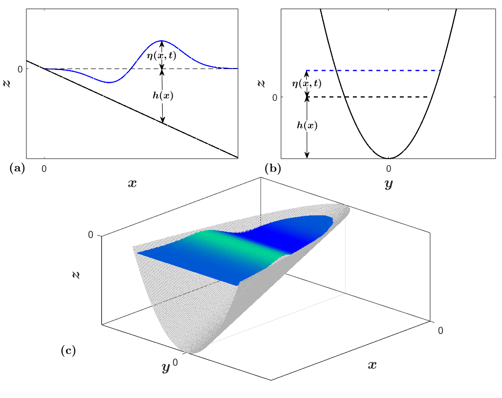
Figure 1: Geometrical representations of a power-shaped bathymetry resembling the case $m=2$. In (a) we have cross sectional view of the $xOz$ plane, in (b) a cross sectional view of the $yOz$ plane, and in (c) a 3-dimensional view of the bay and an $N$-wave.

3 Statement of the direct and inverse problems

In this paper we investigate the following direct problem: knowing the initial displacement of the water $\eta_{0}(x)$ and assuming zero initial velocity of the water, we find the movement of the shoreline $x_{0}(t)$. The direct problem was solved both numerically and analytically by many authors (see the references in the introduction). The corresponding inverse problem then consists of restoring the initial displacement of the water, assuming zero initial velocity and knowing the shoreline movement $x_{0}(t)$ and the time of an earthquake, i.e., zero time. It is worth noting that a non-linear inverse problem, as is the case with our problem, presents several challenges in terms of deriving a solution. The main difficulty is that the shoreline is moving. The Carrier-Greenspan transform allows to reduce the original problem to a linear one on $\mathbb{R}_{>0}$.

Carrier-Greenspan Transform

The Carrier-Greenspan (CG) hodograph transform, introduced in [Carrier & Greenspan (1958)], can be used to linearise (2.1) into a form which can then be solved using Hankel transforms [Courant & Hilbert]. We use the form of the CG transform, originally introduced for power-shaped bays in [Tuck & Hwang (1972)]:

$$\varphi(\tau,\sigma)=u(x,t),\quad\sigma=x+\eta(x,t),\quad\psi(\tau,\sigma)=\eta(x,t)+u^{2}(x,t)/2,\quad\tau=t-u(x,t).$$ (3.1)

Applying (3.1) to (2.1) yields the linear hyperbolic system

$$\begin{split}\partial_{\tau}\psi+\frac{m}{m+1}\sigma\partial_{\sigma}\varphi+\varphi&=0,\\ \partial_{\tau}\varphi+\partial_{\sigma}\psi&=0,\end{split}$$ (3.2)

which is often written as the second order equation

$$\partial^{2}_{\tau}\psi=\frac{m}{m+1}\sigma\partial^{2}_{\sigma}\psi+\partial_{\sigma}\psi.$$ (3.3)

We therefore obtain a linear hyperbolic equation (3.3) from a non-linear system (2.1). Physically, $\sigma$ denotes wave height from the bottom, $\tau$ is a delayed time, $\varphi$ is the flow velocity, and $\psi$ can be called the total energy. The CG transforms main benefit is that the moving shoreline $x_{0}(t)$ is fixed at $\sigma=0$. Nevertheless, the CG transform has some notable drawbacks; for one, the ICs become complicated in the hodograph coordinates, making standard techniques difficult to apply. However, by setting the initial velocity of the wave to be zero, that is $u_{0}(x)=0$, one avoids this issue. While, this premiss is restrictive, it is typical when considering earthquake generated tsunamis. Thus, we assume this condition which is equivalent to $\varphi(0,\sigma)=0$, and so (2.4) becomes

$${\left.\varphi\vphantom{\Bigr{|}}\right\lvert_{\Gamma}}=0,\quad{\left.\psi\vphantom{\Bigr{|}}\right\lvert_{\Gamma}}=\psi_{0}(\sigma)=\eta_{0}(\gamma(\sigma))$$ (3.4)

where $\Gamma$ is the vertical line $(0,\sigma)$ in the hodograph plane and $x=\gamma(\sigma)$ solves $\sigma=\eta(x,t)+x$. Additionally, the regular singularity at $\sigma=0$ causes computational difficulties at the shoreline. Finally, we note that the transformation only works provided it is invertible, i.e. the wave does not break [Rybkin et al. (2021)], so we must surmise this going forward.

4 The Shoreline Equation

In this section we derive what we call the shoreline equation of an arbitrary power-shaped bay. Specifically, we derive an equation relating $\psi(\tau,0)$, the energy of the water at the shoreline, and $\psi(0,\sigma)=\psi_{0}(\sigma)$ the initial displacement of the water. Notably, the direct problem has previously been solved for power-shaped bathymetries (see, for instance, [Garayshin et al. (2016)],[Didenkulova & Pelinovsky (2011)]) and the inverse problem in the narrow case of a plane beach [Rybkin et al. (2023)]. Here the direct problem is solved both analytically, as follows in this section, and numerically, as can be seen in Section 6, to ensure that propagation of the wave is being accounted for as described in [Satake et al. (1987)]. Since the energy at the shoreline can be computed from the movement of the shoreline $x_{0}(t)$, the shoreline equation allows us to easily solve the inverse problem and recover $\eta_{0}(x)$ after converting back into physical space.

We start with the bounded analytical solution to the initial value problem (3.3, 3.4), which is given in [Rybkin et al. (2021)]:

$$\psi(\tau,\sigma)=\sigma^{-\frac{1}{2m}}\int_{0}^{\infty}2k\left(\int_{0}^{\infty}\psi_{0}(s)s^{\frac{1}{2m}}J_{\frac{1}{m}}(2k\sqrt{s})\leavevmode\nobreak\ \mathrm{d}s\right)\cos\left(\sqrt{\frac{m}{m+1}}k\tau\right)J_{\frac{1}{m}}(2k\sqrt{\sigma})\leavevmode\nobreak\ \mathrm{d}k,$$ (4.1)

where $J_{\frac{1}{m}}$ is the Bessel function of the first kind of order $1/m$ and $\Gamma(z)$ is the gamma function. Since $J_{\nu}(z)=z^{\nu}2^{-\nu}/\Gamma\left(\nu+1\right)+{o}(1)$ as $z\to+0$, we obtain

$$\psi(\tau,0)=\frac{2}{\Gamma(\frac{1}{m}+1)}\int_{0}^{\infty}k^{\frac{1}{m}+1}\left(\int_{0}^{\infty}\psi_{0}(s)s^{\frac{1}{2m}}J_{\frac{1}{m}}(2k\sqrt{s})\leavevmode\nobreak\ \mathrm{d}s\right)\cos\left(\sqrt{\frac{m}{m+1}}k\tau\right)\leavevmode\nobreak\ \mathrm{d}k,$$ (4.2)

which after the substitution $\lambda=\sqrt{s}$ and $\widehat{\psi}_{0}(\lambda)=\psi_{0}(\lambda^{2})$ becomes

$$\psi(\tau,0)=\frac{4}{\Gamma(\frac{1}{m}+1)}\int_{0}^{\infty}k^{\frac{1}{m}+1}\left(\int_{0}^{\infty}\widehat{\psi}_{0}(\lambda)\lambda^{\frac{1}{m}+1}J_{\frac{1}{m}}(2k\lambda)\leavevmode\nobreak\ \mathrm{d}\lambda\right)\cos\left(\sqrt{\frac{m}{m+1}}k\tau\right)\leavevmode\nobreak\ \mathrm{d}k.$$ (4.3)

Now, define the modified Hankel transform as

$$\left[\widehat{\mathcal{H}}_{\nu}f(r)\right](k)=k^{-\nu}\int_{0}^{\infty}f(r)J_{\nu}(kr)r^{\nu+1}\leavevmode\nobreak\ \mathrm{d}r.$$ (4.4)

Note that

$$\left[\widehat{\mathcal{H}}_{\nu}f(r)\right](\lambda)=\lambda^{-\nu}\left[\mathcal{H}_{\nu}r^{\nu}f(r)\right](\lambda),$$ (4.5)

where $\mathcal{H}_{\nu}$ is the standard Hankel transform, and so we observe that $\widehat{\mathcal{H}}_{\nu}$ is self-inverse. So, applying (4.4) to (4.3) we have

$$\psi(\tau,0)=\frac{2^{2+\frac{1}{m}}}{\Gamma(\frac{1}{m}+1)}\int_{0}^{\infty}k^{1+\frac{2}{m}}\left[\widehat{\mathcal{H}}_{\frac{1}{m}}\widehat{\psi}_{0}(\lambda)\right](2k)\cos\left(2\pi\xi k\right)\leavevmode\nobreak\ \mathrm{d}k,$$ (4.6)

where $\xi=(\sqrt{m/(m+1)}\tau)/2\pi=:q^{-1}\tau$. Let $g(k)=k^{1+\frac{1}{2m}}\left[\widehat{\mathcal{H}}_{\frac{1}{m}}\widehat{\psi}_{0}(\lambda)\right](2k)$ and denote

$$\left[\mathcal{F}_{c}f(t)\right](\xi)=\int_{0}^{\infty}f(t)\cos(2\pi\xi t)\leavevmode\nobreak\ \mathrm{d}t,$$ (4.7)

as the Fourier cosine transform. Then we obtain

$$\psi(\tau,0)=\frac{2^{2+\frac{1}{m}}}{\Gamma(\frac{1}{m}+1)}\int_{0}^{\infty}g(k)\cos(2\pi\xi k)\leavevmode\nobreak\ \mathrm{d}k=\frac{2^{2+\frac{1}{m}}}{\Gamma(\frac{1}{m}+1)}\left[\mathcal{F}_{c}g(k)\right](\xi)=\frac{2^{2+\frac{1}{m}}}{\Gamma(\frac{1}{m}+1)}\left[\mathcal{F}_{c}k^{1+\frac{1}{2m}}\left[\widehat{\mathcal{H}}_{\frac{1}{m}}\widehat{\psi}_{0}(\lambda)\right](2k)\right](\xi).$$ (4.8)

So (4.8) allows us to solve the direct problem. For that one would need to find $\psi_{0}(\sigma)$ from the Carrier-Greenspan transform as

$$\eta_{0}\left(x\right)=\psi_{0}\left(\sigma\right),\quad\sigma={x+\eta_{0}\left(x\right)},$$ (4.9)

then compute two integral transforms, and finally return to the $(x,t)$ space using the inverse CG transform, which at the shoreline becomes

$$\psi\left(\tau,0\right)=-x_{0}\left(t\right)+\dot{x}_{0}\left(t\right)^{2}/2,\quad\tau=t-\dot{x}_{0}\left(t\right).$$ (4.10)

Solution to the Inverse problem

In this section we invert the transform given in (4.8) in order to solve the inverse problem.

Applying the inverse Fourier cosine transform to (4.8) we obtain

$$\frac{\Gamma(\frac{1}{m}+1)}{2^{2+\frac{1}{m}}}\psi(q\xi,0) =\left[\mathcal{F}_{c}g(k)\right](\xi)$$ (4.11)

$$\frac{\Gamma(\frac{1}{m}+1)}{2^{2+\frac{1}{m}}}\left[\mathcal{F}_{c}^{-1}\psi(q\xi,0)\right](k) =k^{1+\frac{1}{2m}}\left[\widehat{\mathcal{H}}_{\frac{1}{m}}\widehat{\psi}_{0}(\lambda)\right](2k)$$

$$\frac{\Gamma(\frac{1}{m}+1)}{2^{2+\frac{1}{m}}k^{1+\frac{1}{2m}}}\left[\mathcal{F}_{c}^{-1}\psi(q\xi,0)\right](k) =\left[\widehat{\mathcal{H}}_{\frac{1}{m}}\widehat{\psi}_{0}(\lambda)\right](2k).$$

Applying the inverse Hankel transform and utilising the identity [Gradshteyn & Ryzhik (2007)]

$$J_{\nu}(z)=\frac{2\left(\frac{z}{2}\right)^{\nu}}{\Gamma\left(\nu+\frac{1}{2}\right)\sqrt{\pi}}\int_{0}^{1}\cos zs(1-s^{2})^{\nu-\frac{1}{2}}\leavevmode\nobreak\ \mathrm{d}s\quad\text{for }z>0,\leavevmode\nobreak\ \nu>-\frac{1}{2},$$ (4.12)

we obtain

$$\widehat{\psi}_{0}(\lambda)=2\Gamma(1+1/m)\lambda^{-1/m}\int_{0}^{\infty}k^{-1/m}\int_{0}^{\infty}\psi(q\xi,0)\cos 2\pi\xi k\leavevmode\nobreak\ \mathrm{d}\xi J_{1/m}(2k\lambda)\leavevmode\nobreak\ \mathrm{d}(2k)\\ =\frac{8\Gamma(1+1/m)}{\sqrt{\pi}\Gamma(1/m+1/2)}\int_{0}^{\infty}\int_{0}^{\infty}\psi(q\xi,0)\cos(2\pi\xi k)\leavevmode\nobreak\ \mathrm{d}\xi\int_{0}^{1}\cos(2\pi\lambda s)(1-s^{2})^{1/m-1/2}\leavevmode\nobreak\ \mathrm{d}s\leavevmode\nobreak\ \mathrm{d}k\\ =\frac{2\Gamma(1+1/m)}{\lambda\Gamma(1/m+1/2)}\int_{0}^{1}(1-s^{2})^{1/m-1/2}4\int_{0}^{\infty}\int_{0}^{\infty}\psi(q\xi,0)\cos 2\pi k\xi\leavevmode\nobreak\ \mathrm{d}\xi\cos(2k\lambda s)\leavevmode\nobreak\ \mathrm{d}k\leavevmode\nobreak\ \mathrm{d}s\\ =\frac{2\sqrt{\pi}\Gamma(1+1/m)}{\lambda\Gamma(1/m+1/2)}\int_{0}^{\lambda/\pi}\left(1-\frac{\pi^{2}}{\lambda^{2}}\xi\right)^{1/m-1/2}4\int_{0}^{\infty}\int_{0}^{\infty}\psi(q\xi,0)\cos 2\pi k\xi\leavevmode\nobreak\ \mathrm{d}\xi\cos 2\pi k\xi\leavevmode\nobreak\ \mathrm{d}k\leavevmode\nobreak\ \mathrm{d}\xi\\ =\frac{2\sqrt{\pi}\Gamma(1+1/m)}{\lambda\Gamma(1/m+1/2)}\int_{0}^{\lambda/\pi}\left(1-\left(\frac{\pi\xi}{\lambda}\right)^{2}\right)^{1/m-1/2}\psi(q\xi,0)\leavevmode\nobreak\ \mathrm{d}\xi.$$ (4.13)

Upon switching back to variable $\sigma$ one obtains

$$\psi_{0}(\sigma^{2})=\frac{2\sqrt{\pi}\Gamma(1+1/m)}{\sigma^{2}\Gamma(1/m+1/2)}\int_{0}^{\sigma^{2}/\pi}\left(1-\left(\frac{\pi\xi}{\sigma^{2}}\right)^{2}\right)^{1/m-1/2}\psi(\tau,0)\leavevmode\nobreak\ \mathrm{d}\xi.$$ (4.14)

Now denote

$$\left[\mathcal{A}_{\alpha}f(x)\right](s)=\int_{0}^{s}\frac{f(x)\leavevmode\nobreak\ \mathrm{d}x}{(s^{2}-x^{2})^{\alpha}}$$ (4.15)

as the singular Abel type integral of order $\alpha$ as seen in [Deans (2000)]. After a straightforward substitution one obtains that

$$\psi_{0}(\sigma^{2})=\frac{2\Gamma\left(\frac{m+1}{m}\right)}{\Gamma\left(\frac{1}{m}+\frac{1}{2}\right)\sqrt{\pi}}\sigma^{-\frac{4}{m}}\left[\mathcal{A}_{1/2-1/m}\psi\left(\frac{qr}{\pi},0\right)\right](\sigma^{2}).$$ (4.16)

Now we can use (4.16) to solve the inverse problem as follows: from the shoreline movement $x_{0}(t)$ we find ${\psi(\tau,0)=-x_{0}(t)+\dot{x}_{0}(t)^{2}/2}$ and $\tau=t-\dot{x}_{0}(t)$, after that from (4.16) we find $\psi_{0}(\sigma)$, and finally we find ${\eta_{0}(x)=\psi_{0}(\sigma)}$ and ${x=\sigma-\eta_{0}(x)}$

Some Remarks

The transform defined in (4.15) is in fact Erdélyi-Kober fractional integration operator (see for example [Sneddon (1975)]). This operator is closely connected [Erdélyi (1970)] to the Euler-Poisson-Darboux (EPD) equation, which one can obtain from SWE (2.1) by taking in the CG transform (3.1) $\sigma^{2}=x+\eta(x,t)$. Moreover, one can use the CG transform used in [Garayshin et al. (2016)] to obtain the IBVP for the EPD equation, that solves the inverse problem, and after that use the technique laid out in [Erdélyi (1970)] to solve it. The only disadvantage of this approach is that it only applies for $m>2$, while our method works for any positive $m$. In [Erdélyi (1970)] Erdélyi claims, that this restriction can be relaxed to any positive $m$, however we have not investigated that.

It is worth noting that (4.15) has an inverse formula for $\alpha\in(0,1)$ [Deans (2000)], given as

$$\left[\mathcal{A}_{\alpha}^{-1}f(x)\right](s)=\frac{2\sin(\alpha\pi)}{\pi}\frac{\mathrm{d}}{\mathrm{d}s}\int_{0}^{s}\frac{xf(x)\leavevmode\nobreak\ \mathrm{d}x}{(s^{2}-x^{2})^{1-\alpha}}.$$ (4.17)

Thus, for all $m>2$ we can invert (4.16) to obtain (after substituting $s=\sigma^{2}$)

$$\psi(qr/\pi,0)=\frac{\sqrt{\pi}}{\Gamma(1+\frac{1}{m})\Gamma(\frac{1}{2}-\frac{1}{m})}\frac{\mathrm{d}}{\mathrm{d}r}\left[\mathcal{A}_{\frac{m+2}{2m}}s^{\frac{2}{m}}\psi_{0}(s)\right](r).$$ (4.18)

This allows to solve the direct problem using one integral operator, rather then composing two Fourier transform for $m>2$.

Particular cases

In the two most interesting cases, that is the case of the infinite plane beach corresponding to $m=\infty$ and a parabolic bay for $m=2$, our solution can be shown to reduce down to particularly nice forms. For $m=\infty$ we have $q=2\pi$  and so (4.16) easily simplifies to

$$\psi_{0}(\sigma^{2})=\frac{2}{\pi}\left[\mathcal{A}_{\frac{1}{2}}\psi(2r,0)\right](\sigma^{2}).$$ (4.19)

The substitution $\sigma^{\prime}=\sigma^{2}$ and $\tau^{\prime}=\tau/2$ turns (4.19) to the form obtained in [Rybkin et al. (2023)].

For $m=2$ we have $q=\pi\sqrt{6}$, and so (4.16) simplifies to

$$\psi_{0}(\sigma^{2})=\frac{1}{\sigma^{2}}\left[\mathcal{A}_{0}\psi(\sqrt{6}r,0)\right](\sigma^{2})=\frac{1}{\sigma^{2}}\int_{0}^{\sigma^{2}}\psi(\sqrt{6}r,0)\leavevmode\nobreak\ \mathrm{d}r.$$ (4.20)

5 Estimate of the shape of the incoming wave

In this section we give the exact lower bound for the support of the initial water displacement in terms of the shoreline data. First we remind that for a scalar-valued function $f:X\to\mathbb{C}$ the support is the set $\operatorname{supp}f=\left\{x\in X\,\middle|\,f(x)\neq 0\right\}$. For the case $m=2$ we have

$$\psi_{0}(\sigma^{2})=\sigma^{-2}\int_{0}^{\sigma^{2}}\psi(\sqrt{6}r,0)\leavevmode\nobreak\ \mathrm{d}r,$$ (5.1)

and so we deduce that $\inf\operatorname{supp}\psi_{0}(\sigma^{2})=\inf\operatorname{supp}\psi\left(\sqrt{6}r,0\right)$.

For $m>2$ we can use Titchmarsh’s convolution theorem, which states (see [Titchmarsh (1926)] for details) that if

$${\left.(f*g)\vphantom{\Bigr{|}}\right\lvert_{x\in(0,a)}}={\left.\left(\int_{0}^{x}f(t)g(x-t)\leavevmode\nobreak\ \mathrm{d}t\right)\vphantom{\Bigr{|}}\right\lvert_{x\in(0,a)}}=0,$$ (5.2)

and $g(x)>0$ on $(0,a)$, then $f(x)=0$ almost everywhere on $(0,a)$. From (4.18) we have

$$\psi\left(\frac{qr}{\pi},0\right)=C(m)\frac{\mathrm{d}}{\mathrm{d}r}\left(\int_{0}^{r}\left(\psi_{0}(s)s^{\frac{2}{m}}(r+s)^{\frac{2+m}{2m}}\right)(r-s)^{\frac{2+m}{2m}}\leavevmode\nobreak\ \mathrm{d}s\right),$$ (5.3)

and so we deduce that $\inf\operatorname{supp}\psi_{0}(s)\leq\inf\operatorname{supp}\psi\left(\frac{qr}{\pi},0\right)$. The inverse inequality immediately follows from (4.16), and so combining these results we obtain $\inf\operatorname{supp}\psi_{0}(s)=\inf\operatorname{supp}\psi\left(\frac{qr}{\pi},0\right)$.

So we can express the lower bound of the support of $\psi_{0}(\sigma)$. Since $\psi_{0}(\sigma)=\eta_{0}(x)$ and $\sigma=x+\eta_{0}(x)$, we can obtain the exact lower bound of the support $\eta_{0}(x)$, namely $\inf\operatorname{supp}\eta_{0}(x)=\inf\operatorname{supp}\psi_{0}(\sigma)$. In simple language that means that we can express how far from the shore the displacement is at the time of an earthquake.

6 Numerical Computations

In this section we numerically verify our method for recovering $\eta_{0}$ in cases where $m\in\left\{1,2,3,+\infty\right\}$, that is for inclined parabolic bays of different shapes and an infinite sloping beach. In all of bathymetries we consider an “$N$-wave”

$$\eta_{0}(x)=2.5\times 10^{-3}e^{-3.5(x-1.9625)^{2}}-1.25\times 10^{-3}e^{-3.5(x-1.4)^{2}},$$ (6.1)

and a Gaussian wave

$$\eta_{0}(x)=5\times 10^{-3}e^{-(x-3)^{2}},$$ (6.2)

with zero initial velocity. Existing code provided by Rybkin et al. [Rybkin et al. (2021)] was used to generate the shoreline data. We then implemented (4.19) and (4.20) respectively to recover the initial displacements. Comparison of the exact initial wave profiles and those predicted by our model can be seen in Figures 4 and 2. Corresponding shoreline movements can be seen in Figures 5 and 3. It is worth noting that when we consider the same initial displacement for various bathymetries, the amplitude of the shoreline movement decreases as $m$ increases.

Initial Wave Profiles

(a) $m=1$

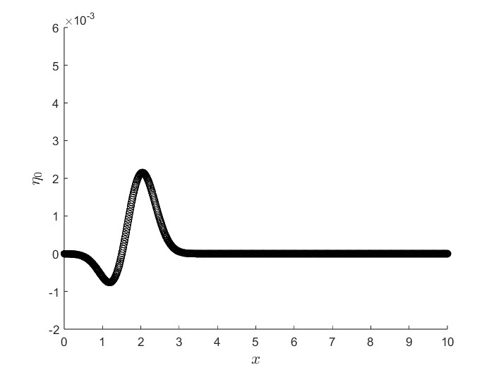
(b) $m=2$

(c) $m=3$

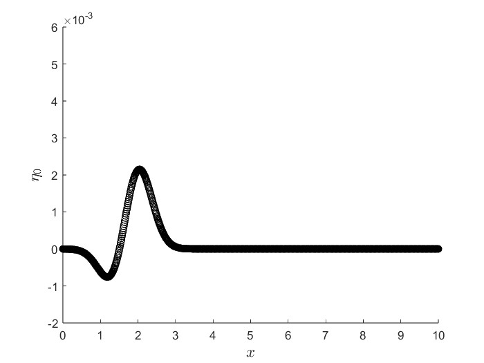
(d) $m=\infty$

Figure 2: A comparison of an initial displacement of an $N$-wave with the displacement predicted by our model for varying power-shaped bays. The solid black line gives the exact initial displacement and the open circles denote the initial displacement predicted by our model.

Vertical Shift Profiles

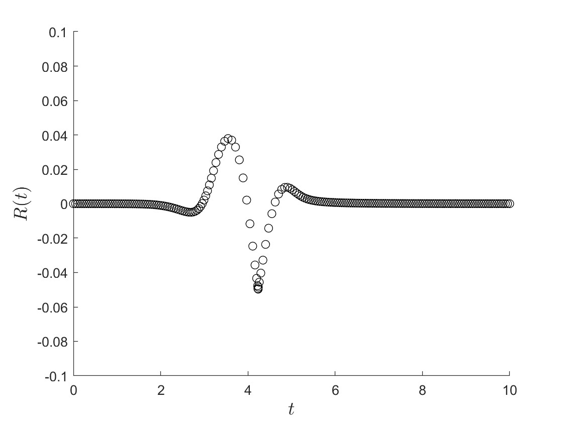
(a) $m=1$

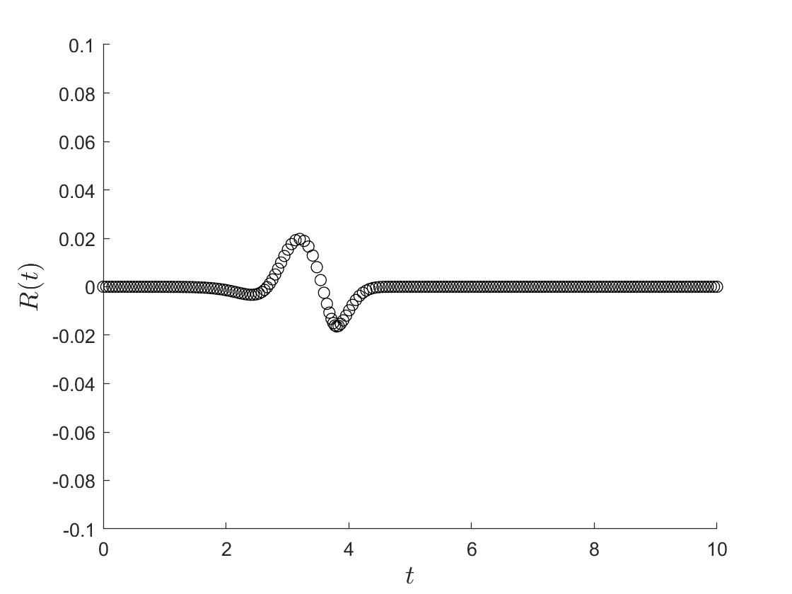
(b) $m=2$

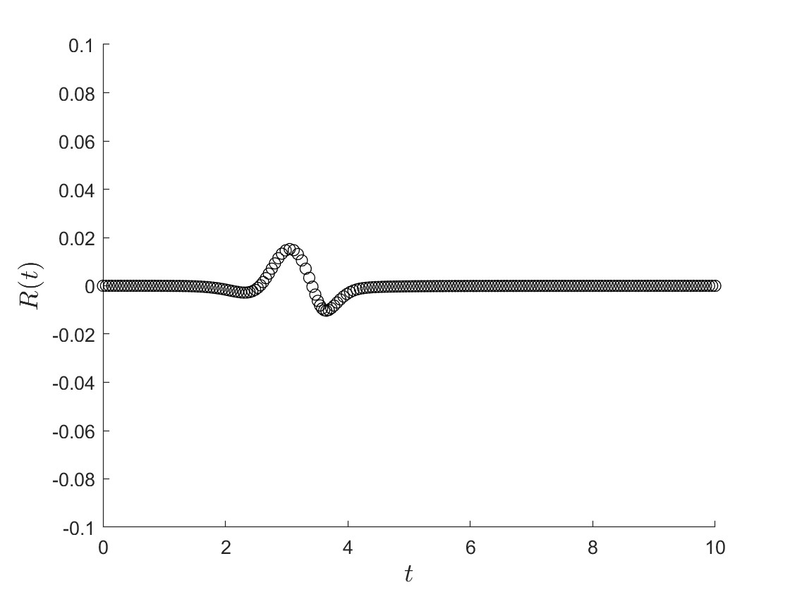
(c) $m=3$

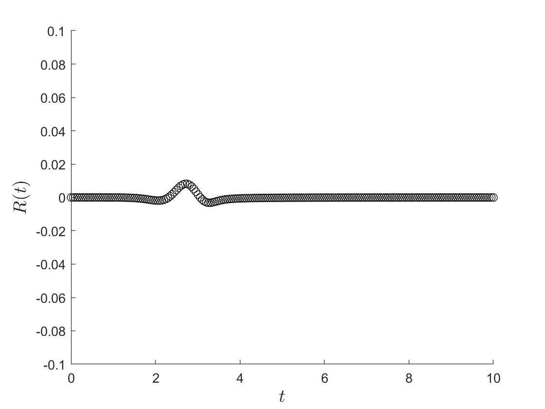
(d) $m=\infty$

Figure 3: Estimated vertical shift for an initial $N$-wave displacement corresponding to various bathymetries, where $R(t)=-x_{0}(t)/\alpha$, where $\alpha=1$.

Initial Wave Profiles

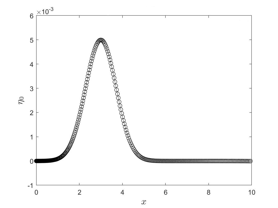
(a) $m=1$

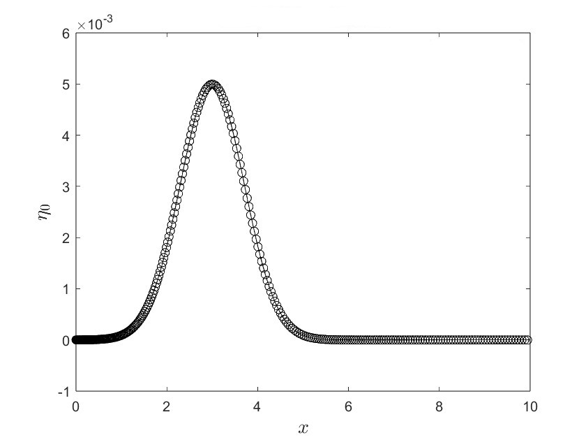
(b) $m=2$

(c) $m=3$

(d) $m=\infty$

Figure 4: A comparison of an initial displacement of an Gaussian wave with the displacement predicted by our model for varying power-shaped bays. The solid black line gives the exact initial displacement and the open circles denote the initial displacement predicted by our model.

Vertical Shift Profiles

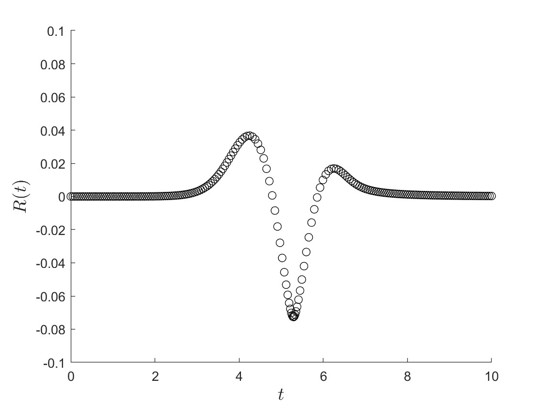
(a) $m=1$

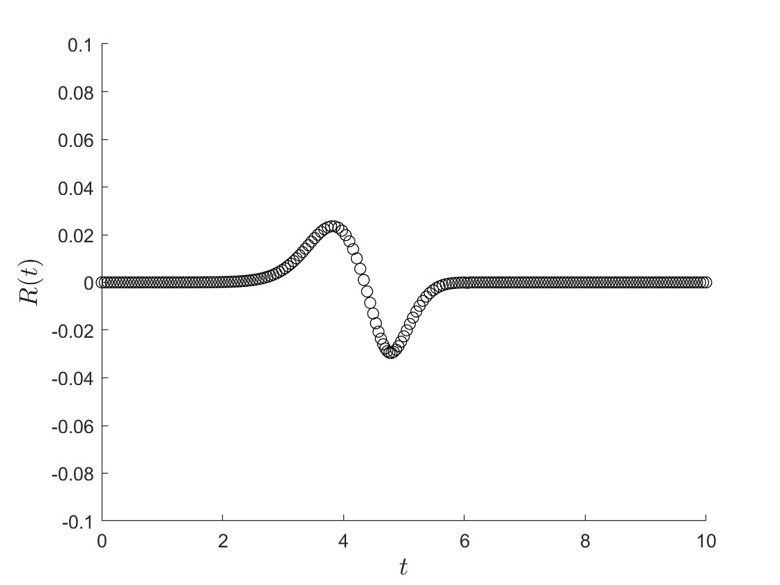
(b) $m=2$

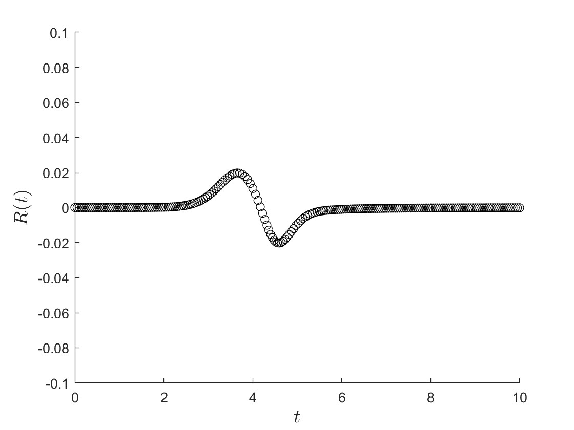
(c) $m=3$

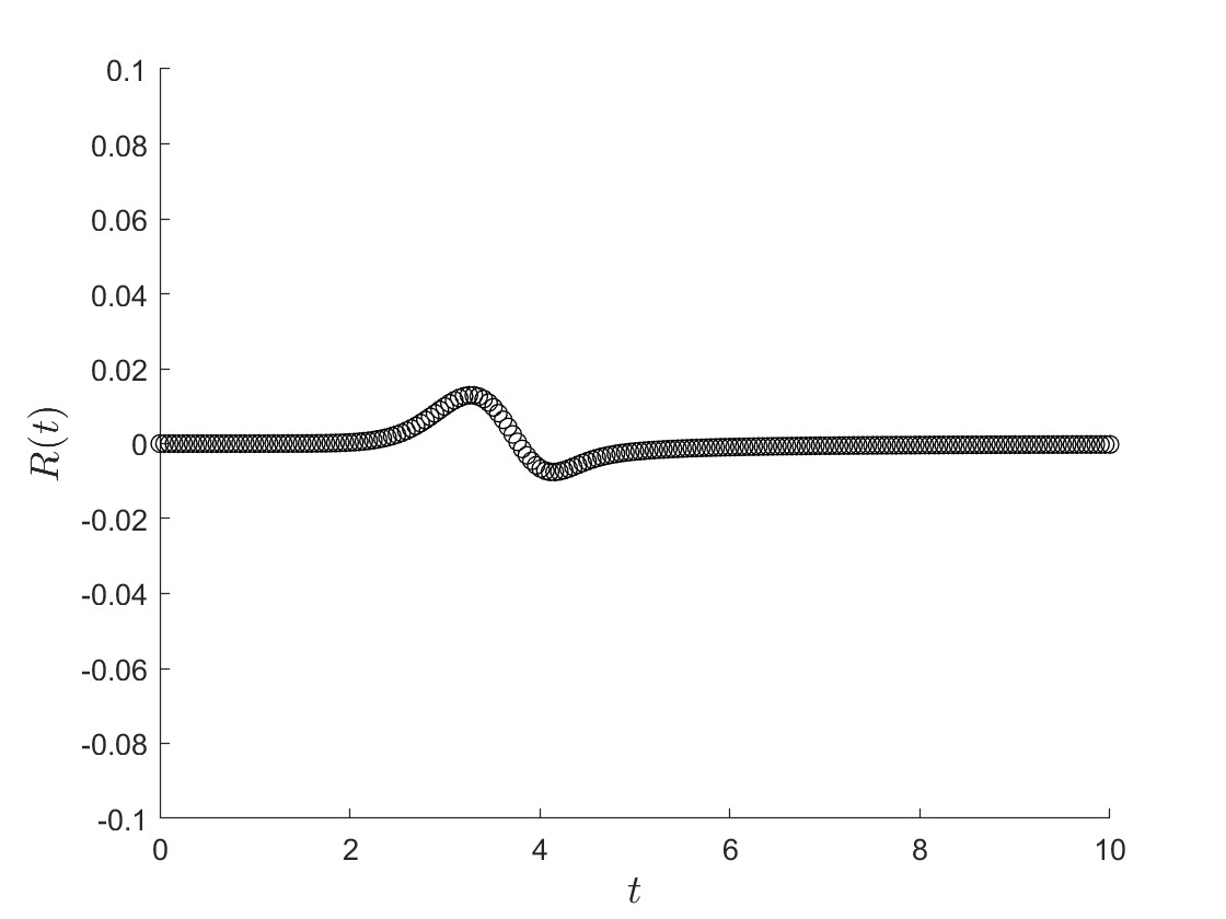
(d) $m=\infty$

Figure 5: Estimated vertical shift for an initial Gaussian wave displacement corresponding to various bathymetries, where $R(t)=-x_{0}(t)/\alpha$, where $\alpha=1$.

It is common when a long tsunami wave is masked by wind waves that have higher frequency. Typically, the tsunami wave length is above 1 kilometre, while wind waves have length of 90 to 180 metres. The integral transform we derived cuts off high-frequency oscillations. To demonstrate that we consider a long wave with added disturbance

$$\eta_{0}(x)=5\times 10^{-3}e^{-(x-2)^{2}}+2.5\times 10^{-4}\sin(50x).$$ (6.3)

Using the same methodology we are again able to recover the initial wave profile (see Fig. 6).

We also consider a noisy shoreline data and recover a more smooth initial displacement (figures 7 and 8)

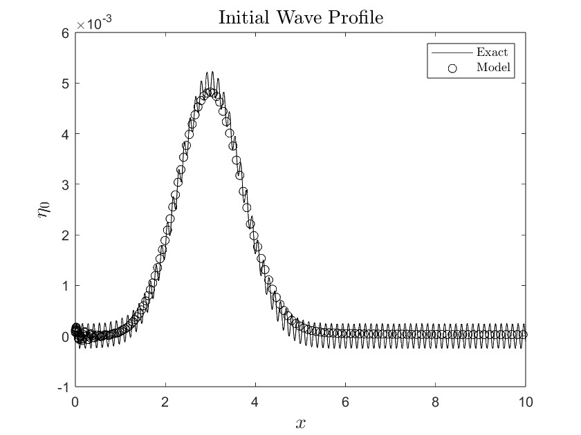
Figure 6: Our model effectively cuts off any high frequency waves, as can be seen with a Gaussian initial wave profile ($m=\infty$).

.

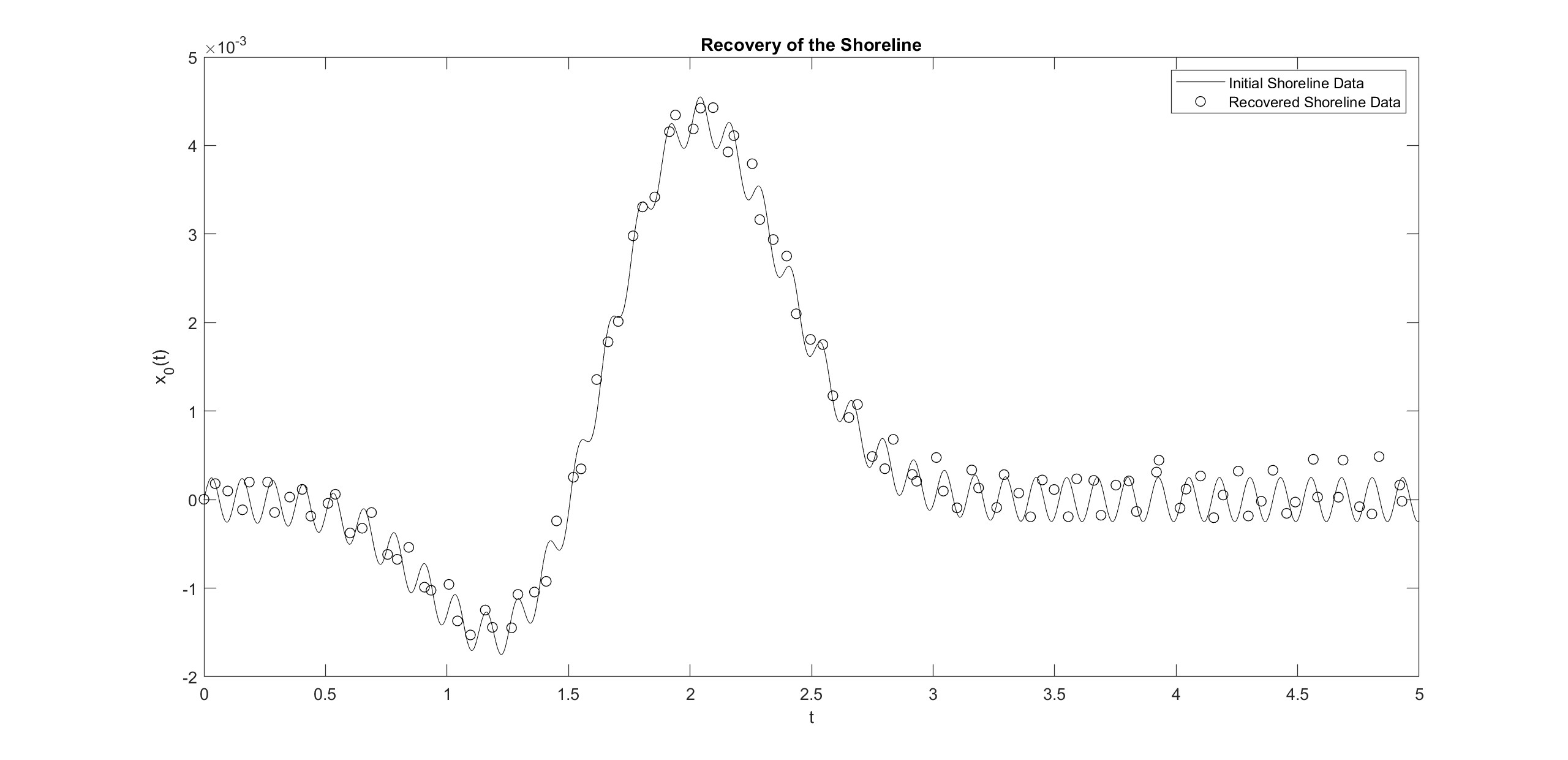
Figure 7: While our numerical model doesn’t remove noise found within the shoreline data, the model is able to cope with the existence of noise and recover it’s behaviour. In this case, our model begins by taking an analytical shoreline function with noise, given by $x_{0}(t)=5\times 10^{-3}e^{-3.5(t-1.9625)^{2}}-2.5\times 10^{-3}e^{-3.5(t-1.4)^{2}}+2.5\times 10^{-4}\sin(50t)$. This $x_{0}(t)$ is utilised to compute $\eta_{0}$ through the inverse problem. Subsequently, the model verifies the validity of this ensuring that the $\eta_{0}$ gained by recovering $x_{0}(t)$ through the direct problem directly matches the analytical $x_{0}(t)$ used to begin the computations. (Done in the case $m=2$)

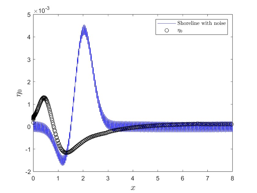
Figure 8: The model appears to reduce high frequency noise. Here we took the shoreline to be $x_{0}(t)=5\times 10^{-3}e^{-3.5(t-1.9625)^{2}}-2.5\times 10^{-3}e^{-3.5(t-1.4)^{2}}+2.5\times 10^{-4}\pi\sin(50\pi t)$ and then computed $\eta_{0}$ using (4.19) which recovered a relatively smooth curve, as seen above.

7 Conclusions

We have put forth and solved an inverse problem for tsunami in power shaped bays assuming zero initial velocity. While not considered here, we believe that a similar inverse problem can be treated in the case where the initial velocity is given as a function of the initial displacement, e.g., in the important case where $u_{0}=-(2\sqrt{x+\eta_{0}}-2\sqrt{x})$. Indeed, our preliminary results show this to be possible in the plane beach bathymetry. We hope to return to this case in a future work.

Our results here consider a tsunami wave with source an arbitrary distance from the shoreline. However, this is a highly idealised situation. In practice dispersion can only be ignored when the wave is close to the shoreline. This suggests a more practical inverse problem where we have a finite bathymetry, that is $x\leq L$ for $L>0$ and attempt to recover the wave at $L$. This is a boundary value problem and the techniques developed in [Antuono & Brocchini (2007)] and [Rybkin et al. (2021)] may be used to derive a shoreline equation. Finally we note that our inversion method can be readily adjusted to the data read from a mareograph which is close to the shore. Indeed, using the angle of inclination the mareograph readings can be converted into a displacement of the shoreline.

8 Acknowledgements

This work was done as part of the 2023 summer REU program run by Dr. Alexei Rybkin and was supported by NSF grant DMS-2009980. Dr. Efim Pelinovsky thanks a support from RSF 22-17-00153. Oleksandr Bobrovnikov acknowledges support from Alaska EPSCoR NSF award #OIA-1757348 and DMS-2009980. We also thank Dr. Ed Bueler for his valuable discussions of the problem with us. We also thank the UAF DMS for hosting us.

References

- [Abe (1973)] Abe, K. 1973 Tsunami and mechanism of great earthquakes. Phys. Earth Planet. Inter., 7(2), 143-153.
- [Antuono & Brocchini (2007)] Antuono, M. and Brocchini, M. 2007 The boundary value problem for the non-linear shallow water equations. Stud. Appl. Math., 119, 73-93.
- [Aydin (2020)] Aydin, B. 2020 On open boundary conditions for long wave equation in the hodograph plane. Phys. Lett. A, 384(13) 126258, 7.
- [Bueler-Faudree et al. (2022)] Bueler-Faudree, T., Delamere, S., Dutykh, D., Rybkin, A., Suleimani, A. 2022 Fast shallow water-wave solver for plane inclined beaches. SoftwareX, 17, 100983.
- [Carrier & Greenspan (1958)] Carrier, G. and Greenspan, H. 1958 Water waves of finite amplitude on a sloping beach. J. Fluid Mech., 1, 97–109.
- [Carrier et al. (2003)] Carrier, G., Wu, T., and Yeh, H. 2003 Tsunami run-up and draw-down on a plane beach. J. Fluid Mech., 475, 79–99.
- [Courant & Hilbert] Courant, R., and Hilbert, D. Methods of Mathematical Physics, vol. 2. WILEY-VCH Verlag GmbH & Co, (1989).
- [Deans (2000)] Deans, S. 2000 Radon and Abel transforms. Transforms and Applications Handbook, Second Edition, 8-1–8-51.
- [Didenkulova & Pelinovsky (2011)] Didenkulova, I. and Pelinovsky, E. 2011 Non-linear wave evolution and runup in an inclined channel of a parbolic cross-section. Phys. Fluids, 23(8) 086602.
- [Didenkulova et al. (2008)] Didenkulova, I., Pelinovsky, E., Soomere, T. 2008 Run-up characteristics of tsunami waves of “unknown” shapes. Pure Appl. Geophys. 165. 2249–2264.
- [Dorbokhotov et al. (2017)] Dobrokhotov, S. Yu., Nazaikinskii, V.E. and Tolchennikov, A.A. 2017 Uniform asymptotics of the boundary values of the solution in a linear problem on the run-up of waves on a shallow beach. Math. Notes 101, pp. 802–814.
- [Erdélyi (1970)] Erdélyi, A. 1970 On the Euler-Poisson-Darboux equation. J. Anal. Math. 23, pp. 89–102.
- [Fujii et al. (2011)] Fujii, Y., Satake, K., Sakai, S., Shinohara, M. and Kanazawa,T. 2011 Tsunami source of the 2011 off the Pacific coast of Tohoku earthquake. Earth Planets Space, 63, pp. 815–820.
- [Garayshin et al. (2016)] Garayshin, V.V., Harris, M.W., Nicolsky, D.J., Pelinovsky, E.N. and Rybkin, A.V. 2016 An analytical and numerical study of long wave run-up in U-shaped and V-shaped bays. Appl. Math. and Comp., 297, pp. 187-197.
- [Gradshteyn & Ryzhik (2007)] Gradshteyn, I.S. and Ryzhik, I.M. 2007 Table of Integrals, Series, and Products. Seventh edition, Academic Press.
- [Hartle et al. (2021)] Hartle, H., Rybkin, A., Pelinovsky, E., and Nicolsky, D. 2021 Robust computations of runup in inclined U- and V-shaped bays. Pure Appl. Geophys., 178, pp. 5017-5029.
- [Johnson (1997)] Johnson, R.S. 1997 A modern introduction to the mathematical theory of water waves. Cambridge University Press.
- [Kânoğlu (2004)] Kânoğlu, U. 2004 Non-linear evolution and runup-drawdown of long waves over a sloping beach. J. Fluid Mech., 513, pp. 363-372.
- [Kânoğlu & Synolakis (2006)] Kânoğlu, U. and Synolakis, C. Initial value problem solution of non-linear shallow water-wave equations. Phys. Rev. Lett., 97 , 148501.
- [Levin & Nosov (2016)] Levin, B. and Nosov, M. 2016 Physics of Tsunamis. Second Edition, Springer.
- [Løvholt et al. (2012)] Løvholt, F., Pedersen, G., Bazin, S., Kühn, D,. Bredesen, RE., and Harbitz, C. Stochastic analysis of tsunami runup due to heterogeneous coseismic slip and dispersion. Journal of Geophysical Research, 117, C03047.
- [Nicolsky et al. (2018)] Nicolsky, D., Pelinovsky, E., Raz, A., and Rybkin, A 2018 General initial value problem for the non-linear shallow water equations: Runup of long waves on sloping beaches and bays Phys. Lett. A, 381(38), pp. 2738-2743.
- [Okada et al. (1985)] Okada, Y. 1985 Surface Deformation Due to Shear and Tensile Faults in a Half-Space Bulletin of the Seismological Society of America, 75, pp. 1135-1154.
- [Okada et al. (1992)] Okada, Y. 1992 Internal deformation due to shear and tensile faults in a half-space Bulletin of the Seismological Society of America, 82, pp. 1018-1040.
- [Pelinovsky and Mazova (1992)] Pelinovsky, E., and Mazova, R. 1992 Exact analytical solutions of nonlinear problems of tsunami wave run-up on slopes with different profiles Natural Hazards, vol. 6, N. 3, pp. 227-249.
- [Rybkin et al. (2014)] Rybkin, A., Pelinovsky E., and Didenkulova, I. 2014 Non-linear wave run-up in bays of arbitrary cross-section: generalization of the Carrier-Greenspan approach J. Fluid Mech., 748, pp. 416-432.
- [Rybkin et al. (2019)] Rybkin, A. 2019 Method for solving hyperbolic systems with initial data on non-characteristic manifolds with applications to the shallow water wave equations Appl. Math. Lett., 93, pp. 72-78.
- [Rybkin et al. (2021)] Rybkin, A., Nicolsky, D., Pelinovsky, E., Buckel, M. 2021 The generalized Carrier-Greenspan transform for the shallow water system with arbitrary initial and boundary conditions Water Waves, 3, pp. 267-296.
- [Rybkin et al. (2023)] Rybkin, A., Pelinovsky, E., Palmer, N. 2023 Inverse problem for the nonlinear long wave runup on a plane sloping beach Appl. Math. Lett., 145.
- [Satake et al. (1987)] Satake, K. 1987 Inversion of tsunami waveforms for the estimation of heterogeneous fault motion of large submarine earthquakes – the 1968 Tokachi-Oki and 1983 Japan Sea earthquakes J. Geophys. Res., 94, pp. 5627-5636.
- [Satake et al. (2021)] Satake, K. 2021 Inverse problems of tsunamis Complexity in Tsunamis, Volcanoes, and their Hazards, pp. 71-89.
- [Shimozono (2016)] Shimozono, T. 2016 Long wave propagation and run-up in converging bays. J. Fluid Mech., 798, pp. 457–484.
- [Sneddon (1975)] Sneddon, I.N. 1975 The use in mathematical physics of Erdélyi-Kober operators and of some of their generalizations. In Fractional Calculus and Its Applications, ed Ross, B., vol 457, Lecture Notes in Mathematics. Springer. https://doi.org/10.1007/BFb0067097
- [Synolakis (1987)] Synolakis, C. 1987 The runup of solitary waves. J. Fluid Mech., 185, pp. 523-545.
- [Synolakis et al. (1988)] Synolakis, C.E., Deb, M.K., and Skjelbreia, J.E. 1988 The anomalous behavior of the run-up of cnoidal waves. Phys. Fluids, 31(1), pp. 3-5.
- [Synolakis & Bernard (2006)] Synolakis, C., Bernard, E. 2006 Tsunami science before and beyond Boxing Day 2004. Philos. Trans. Royal Soc. A, 364, pp. 2231-2265.
- [Tadepalli & Synolakis (1994)] Tadepalli, S., Synolakis, C. 1994 The runup of -waves. Proc. R. Soc. A, 445, pp. 99-112.
- [Titchmarsh (1926)] Titchmarsh, E. 1926 The Zeros of Certain Integral Functions. Proc. Lond. Math. Soc., s2-25(1), pp. 283–302.
- [Tinti & Tonini (2005)] Tinti S., Tonini R. 2005 Analytical evolution of tsunamis induced by near-shore earthquakes on a constant-slope ocean. J. Fluid Mech., 535, pp. 33-64.
- [Titov et al. (2016)] Titov, V., Kânoğlu, U., and Synolakis, C. 2016 Development of MOST for real-time tsunami forecasting. J. Waterw. Port Coast. Ocean Eng., 142(6) , 03116004.
- [Tuck & Hwang (1972)] Tuck, E., Hwang, L. 1972 Long wave generation on a sloping beach. J. Fluid Mech., 51, pp. 449-461.