MS-0000-0000.00

Xu, Lee, and Tan

Algorithmic Collusion or Competition

Algorithmic Collusion or Competition: the Role of Platforms’ Recommender Systems

Xingchen (Cedric) Xu Michael G. Foster School of Business, University of Washington, Seattle, WA 98195, xcxu21@uw.edu Stephanie Lee Michael G. Foster School of Business, University of Washington, Seattle, WA 98195, stelee@uw.edu Yong Tan Michael G. Foster School of Business, University of Washington, Seattle, WA 98195, ytan@uw.edu Recent academic research has extensively examined algorithmic collusion resulting from the utilization of artificial intelligence (AI)-based dynamic pricing algorithms. Nevertheless, e-commerce platforms employ recommendation algorithms to allocate exposure to various products, and this important aspect has been largely overlooked in previous studies on algorithmic collusion. Our study bridges this important gap in the literature and examines how recommendation algorithms can determine the competitive or collusive dynamics of AI-based pricing algorithms. Specifically, two commonly deployed recommendation algorithms are examined: (i) a recommender system that aims to maximize the sellers’ total profit (profit-based recommender system) and (ii) a recommender system that aims to maximize the demand for products sold on the platform (demand-based recommender system). We construct a repeated game framework that incorporates both pricing algorithms adopted by sellers and the platform’s recommender system. Subsequently, we conduct experiments to observe price dynamics and ascertain the final equilibrium. Experimental results reveal that a profit-based recommender system intensifies algorithmic collusion among sellers due to its congruence with sellers’ profit-maximizing objectives. Conversely, a demand-based recommender system fosters price competition among sellers and results in a lower price, owing to its misalignment with sellers’ goals. To elucidate the mechanism, we introduce a price deviation for a seller and observe the ensuing behaviors of all the sellers. We find that different recommender systems’ functions in exposure allocation can act as punishment instruments, guiding sellers toward distinct equilibrium prices. Extended analyses suggest the robustness of our findings in various market scenarios. Overall, we highlight the importance of platforms’ recommender systems in delineating the competitive structure of the digital marketplace, providing important insights for market participants and corresponding policymakers.

algorithmic pricing; competition; collusion; reinforcement learning; recommender systems

1 Introduction

With the advancement of technologies and machine learning algorithms, the usage of automated pricing systems has dramatically increased. For example, a substantial proportion (30%) of residential properties in the United States currently employ RealPage software, which offers instantaneous suggestions for optimal rent rates (Calder-Wang and Kim 2023). Artificial Intelligence (AI)-driven programs, particularly those rooted in reinforcement learning techniques, have emerged as prevalent and compelling alternatives to conventional pricing models. These AI-powered systems require minimal human intervention and possess remarkable adaptability to swiftly changing economic landscapes.

Nevertheless, both researchers and policymakers have expressed concerns regarding the potential detrimental impact of these algorithms on consumers, manifesting in the form of algorithmic collusion. Algorithmic collusion refers to how algorithms can develop the capacity to establish supra-competitive prices through repeated interactions, even in the absence of explicit guidance or communication (Calvano et al. 2020a). The rise of algorithmic collusion presents a regulatory challenge, as current antitrust policies primarily target explicit agreements among humans and lack comprehensive guidelines to effectively identify and address this emerging issue (Harrington 2018).

A growing body of literature has explored algorithmic collusion using theoretical and experimental approaches (Hansen et al. 2021, Calvano et al. 2020b), and empirical studies have investigated the impact of AI adoption on pricing dynamics (Calder-Wang and Kim 2023, Wieting and Sapi 2021, Assad et al. 2020). Despite this, the prior literature on algorithmic collusion has largely overlooked how online marketplaces commonly utilize recommender systems, which alter product exposure and thereby influence sellers’ profits and pricing strategies (Zhang et al. 2019). Recognizing this important absence in the literature, we aim to bridge the gap by examining the research question of how recommender systems modulate sellers’ interactions and consequently reshape price equilibrium.

Addressing this research question theoretically can be challenging, because the stochastic process arising from interactions among multiple reinforcement learning algorithms is still mathematically intractable. Consequently, we employ the numerical method proposed by Calvano et al. (2020b) and establish a Q-learning-based model where sellers engage in recurrent interactions within an online marketplace. Differing from prior studies, which assume that consumers evaluate all the products on the market (Calvano et al. 2020b), our study integrates recommender systems into our model and examines a setting wherein each consumer receives recommendations for a subset of products and subsequently evaluates these offerings. This premise resonates with the fact that most online marketplaces employ recommender systems to alleviate the concern that showing too many products overwhelms consumers’ cognitive capacity and causes an information overload problem (Zhang et al. 2019).

Different platforms utilize varying business models and optimization goals for their recommender systems, necessitating the consideration of two distinct commonly deployed recommender systems: profit-based and demand-based. The profit-based recommender systems aim to maximize total profits among all the sellers (Chen et al. 2008), and align with platforms that derive commission fees from a percentage of sellers’ profits, such as Amazon. Conversely, demand-based recommender systems optimize the total number of purchases and are typical in platforms that generate revenue through per-order service fees, such as UberEats’ delivery fees (Kang and McAuley 2018). Although some platforms may combine these two models, examining two distinct cases of profit-based and demand-based recommender systems can illustrate the impact of differing recommender system goals on pricing dynamics and equilibrium. We also consider a third recommendation system, wherein exposure is equally distributed, mirroring the random assignment of product bundles to customers. For each recommendation policy, simulations are conducted where, in each time period, sellers simultaneously determine prices using Q-learning. Subsequently, the platform’s algorithm dictates the consumer visibility for each product bundle, enabling the realization of profits and subsequent updates to the sellers’ Q matrix for future pricing decisions.

Our experiments reveal how different recommender systems’ exposure adjustment strategies significantly affect pricing directions and the ultimate price equilibrium. Specifically, profit-based recommender systems amplify algorithmic collusion and elevate market prices. This occurs because the profit-based recommender system’s objective is congruent with the sellers’ objective, and its ability to allocate exposure incentivizes the sellers to adopt a collusive price. Conversely, as the demand-based recommender system does not synchronize with the sellers’ objective of profit maximization, its function in distributing exposure promotes competition, culminating in a non-collusive and lower equilibrium price. In exploring potential mechanisms behind the observed equilibrium, we demonstrate that, depending on the recommender systems employed by the platform (i.e., profit-based vs. demand-based), sellers converge to, and remain at, different equilibrium prices due to exposure penalties induced by their respective recommender systems. We also show that our findings are robust across various setups. Consequently, our study is among the first to provide experimental evidence that illuminates the critical role of platforms’ recommender systems in molding algorithmic pricing in online marketplaces. These results contribute to the fields of algorithmic pricing, recommender systems, and competition policies, extending pertinent implications for both stakeholders engaged in the market and corresponding regulatory authorities.

2 Related Literature and Theoretical Contributions

By creatively integrating recommender systems into the repeated competition game among sellers who employ AI-driven pricing algorithms, our study contributes to the literature on artificial intelligence (AI), recommender systems, and competition policy.

2.1 Economics of Artificial Intelligence and Algorithmic Collusion

Broadly speaking, our study is situated within the domain of the economics of AI, wherein economic principles are applied to understand and enhance AI techniques and architectures (Agrawal et al. 2019). More specifically, this study makes a significant contribution to the burgeoning research on algorithmic collusion. With the prevalence of learning algorithms, scholars have investigated the impact of these algorithms on market competition and price equilibrium when employed for automated pricing. A seminal paper demonstrates that the adoption of Q-learning algorithms can result in supra-competitive prices (Waltman and Kaymak 2008). Theoretical studies have complemented the experimental findings by positing that learning algorithms may decipher competitors’ behavior, leading to repeated collusion (Salcedo 2015). Other recent studies propose an alternative explanation: algorithms can acquire a punishment policy that discourages deviations, thereby sustaining collusive prices at profitable levels (Klein 2021, Assad et al. 2020, Calvano et al. 2019). Empirical evidence of algorithmic collusion has also been documented, supporting instances of correlated prices among multiple vendors(Calder-Wang and Kim 2023, Wieting and Sapi 2021, Assad et al. 2020).

Although the research in algorithmic collusion is active, it is noteworthy that existing research on collusion in algorithmic pricing has not thoroughly considered the influence of the platform’s recommendation systems, which directly impact product exposure and profitability in the online marketplace. This study makes a novel contribution to the algorithmic collusion literature by demonstrating that the platform’s recommendation algorithm plays a pivotal role in shaping the competitive landscape of the market and influencing the degree of collusion among sellers. The study also offers an alternative explanation for the observed correlated prices in empirical studies, suggesting that the platform’s recommendation mechanism potentially drives this correlation. By exploring this previously overlooked factor, this research sheds light on the interplay between algorithmic pricing, platform recommendations, and collusion dynamics, providing valuable insights into the functioning of modern digital markets.

2.2 Recommender Systems

By examining the interaction between recommender systems and pricing algorithms, we also contribute to the ongoing literature on recommender systems. Previous studies of recommender systems have typically treated product pricing as an exogenous variable, with a handful of exceptions that have analytically explored the effect of such systems on pricing decisions and market equilibrium in a largely static manner (Zhou and Zou 2023, Li et al. 2020). Therefore, we are among the first researchers to examine the potential of recommender systems to induce dynamic shifts in sellers’ algorithmic pricing strategies. The recent prior literature has consistently shown that algorithmic pricing, irrespective of algorithmic complexity or the nuances of market structures, can potentially disadvantage consumers (Abada and Lambin 2023, Hansen et al. 2021, Calvano et al. 2020b). However, existing research predominantly examines algorithmic pricing within a static market context, typically employing the logit demand model. Different from the prior literature, our study introduces a novel viewpoint, underscoring the critical role of recommender systems in shaping product exposure, which in turn influences the interactions among pricing agents. Additionally, our analyses call for a more comprehensive exploration of intermediaries’ effects on market agents’ responses (Banchio and Skrzypacz 2022).

2.3 Competition Policy and Antitrust Regulation

Our research also relates to the scholarly discourse on competition policies and antitrust regulations, which aims to advance competitive environments, mitigate unwarranted monopolistic practices, and augment societal well-being (Parker et al. 2020, Evans 2003). Specifically, this paper contributes to two streams of literature on antitrust: (i) the effect of algorithms on competition and (ii) the effect of intermediaries on competition.

First, with the proliferation of artificial intelligence and automatic pricing, antitrust policymakers have expressed concerns about the possibility of algorithms acquiring collusion tendencies, which would consequently lead to adverse effects on consumer welfare (Robertson 2022, Colangelo 2021, Fzrachi and Stucke 2019, Schwalbe 2018). In this stream of literature, the delineation of responsibility for supra-competitive prices is still unclear and debatable. Existing regulations are deemed inadequate, as the current operational policies mainly address direct communications among market participants rather than algorithmic pricing and collusion.

Furthermore, extant antitrust scholarship has underscored the significance of intermediaries within the competitive framework (Edelman and Wright 2015), especially following the popularity of online platforms (Tan and Zhou 2021). Nevertheless, the prior literature has not yet adequately examined the influence wielded by intermediaries’ algorithms within the algorithmic competitive landscape among vendors. Therefore, we consolidate these two subdomains of the antitrust literature, highlighting the manner in which platform recommendation systems can configure price equilibrium within online platforms. As a result, policy architects may consider interventions at the platform level, rather than at the level of individual sellers, as a strategy to ameliorate algorithmic collusion.

3 Dynamic Pricing Competition Moderated by the Platform’s Recommendation

Despite its significance, the role of the platform in algorithmic pricing has been largely overlooked in prior research. In this section, we develop and introduce a dynamic pricing competition framework that incorporates the effect of the platform’s recommendation system. We present a comprehensive exposition of the economic framework, the seller’s algorithm, the platform’s algorithm, and various other pertinent elements.

3.1 Economic Environment

Following Calvano et al. (2020b), we utilize the conventional price competition setting, which involves an infinitely repeated pricing game where all firms make simultaneous decisions based on observed histories. Diverging from previous research, our model newly incorporates a platform’s recommendation system; in each stage, the platform allocates the exposure of various products, which is defined by the proportion of consumers exposed to different product bundles.

Specifically, the marketplace encompasses $n$ ($i=1,2,\ldots,n$) differentiated products, whose prices $p_{i}^{t}$ are dynamically adjusted by sellers at each period $t$, and an external good with a constant utility. Given the operational context wherein sellers only fulfill the role of establishing goods’ prices, they are correspondingly denoted as “pricing agents.” Furthermore, the platform generates $m$ bundles denoted by $j=1,2,\ldots,m$, each of which comprises products chosen from the entire product list, and the number of products within each bundle fits the cognitive capacity of consumers. Subsequently, every consumer is recommended one bundle by the platform. Consumers will then consider and evaluate all the products in the recommended bundle. For instance, in a market with only three products, and the platform intending to suggest two products to each consumer, there would be three potential bundles. This configuration aligns with the design of a recommender system that aims to alleviate information overload by narrowing down consumers’ consideration sets (Zhang et al. 2019). By manipulating the proportion of consumers who can view bundles involving a particular product, the platform can determine the exposure and competition structure for each product. The exposure of each bundle at period $t$ is defined by $x_{j}^{t}\in[0,1]$, and $\sum_{j=1}^{m}x_{j}^{t}=1$.

Henceforth, the consumers recommended with the same bundle can be regarded as a sub-market. In order to characterize the demand pertaining to each product within each bundle (sub-market), we employ the logit demand model. The logit demand model has been extensively employed in previous algorithmic collusion studies and empirical works, showcasing its adaptability to various industries (Calvano et al. 2020b). Within the sub-market that recommends bundle $j$ consisting of a set of differentiated products $B_{j}$ and an outside good, the demand for product $i$ at period $t$ when $i\in B_{j}$ is given by

$$d_{i,j}^{t}=x_{j}^{t}*\frac{e^{\frac{{\alpha_{i}-p_{i}^{t}}}{\mu}}}{{\sum_{k\in B_{j}}e^{\frac{{\alpha_{k}-p_{k}^{t}}}{\mu}}+e^{\frac{\alpha_{0}}{\mu}}}}$$ (1)

Here, the parameters $\alpha_{i}$ represent quality indexes for each product within the bundle, capturing vertical differentiation. The parameter $\mu$ reflects the degree of horizontal differentiation where perfect substitution is achieved as $\mu$ approaches $0$. The denominator of the equation represents the exponential sum over all products’ consumption utilities within the bundle $B_{j}$ along with the outside good, characterized by the quality index $\alpha_{0}$.

Hence, the demand for product $i$ in period $t$ corresponds to the aggregate of its individual demands across all the bundles that include it:

$$d_{i}^{t}=\sum_{i\in B_{j}}d_{i,j}^{t}$$ (2)

After assuming a constant marginal cost for each product $i$, we derive the profit incurred by each product $i$ in period $t$ as follows:

$$r_{i}^{t}=(p_{i}^{t}-c_{i})*d_{i}^{t}$$ (3)

3.2 Q-Learning Adopted by Sellers

In the algorithmic collusion literature, Q-learning is used as the archetypal algorithm for examining pricing games, even amidst the progress made in reinforcement learning (Dou et al. 2023, Wang et al. 2023, Colliard et al. 2022, Banchio and Skrzypacz 2022). This preference for the classical Q-learning approach is based on a multitude of compelling justifications (Calvano et al. 2020b, Waltman and Kaymak 2008). First, Q-learning enjoys widespread adoption in practical applications and serves as the foundational basis for numerous state-of-the-art (deep) reinforcement learning algorithms, including but not limited to Deep Q Network (Mnih et al. 2015), Double Deep Q Network (Van Hasselt et al. 2016), and more sophisticated variants that integrate Deep Neural Networks with Tree Search (Silver et al. 2016). Therefore, Q-learning can help yield insights into various algorithmic pricing models that leverage Q-learning’s adaptations. Second, one advantage of the Q-learning algorithm lies in its simplicity, which allows for a full characterization with a significantly reduced number of parameters when compared to algorithms based on neural networks. This characteristic facilitates easier parameter tuning and interpretation of their impact on the model’s performance and behavior. Third, another strength of Q-learning is its capacity to operate without prior knowledge of the economic environment it interacts with. As a result, Q-learning better reflects the real-world scenarios faced by sellers, who often possess limited knowledge about the entirety of the market. This aspect enhances the applicability of the pricing model, making it more suitable to practical situations.

We now provide detailed descriptions of our Q-learning algorithm and introduce relevant notations for our setting. Following the original work on Q-learning, we use this algorithm as a means to update the Q table and ascertain the optimal strategy within the framework of Markov decision processes (Watkins 1989). In each discrete period $t$, the pricing agent $i$ (i.e., seller $i$ on the platform) observes the current state variable denoted as $s^{t}$ and selects a pricing action $p_{i}^{t}$ from a set of feasible actions $A$. Even though the pricing agent has access to the historical pricing data, to streamline calculations and maintain consistency with prior studies, we consider a one-period memory (Calvano et al. 2020b), resulting in the state being represented solely by the prices of all products in the previous period: $s^{t}=(p_{1}^{t-1},...,p_{n}^{t-1})$. Following this, the pricing agent receives a reward (profit) denoted as $r_{i}^{t}$ from an undisclosed economic environment, while simultaneously observing the complete set of prices transitioning to the subsequent period, represented as $s^{t+1}=(p_{1}^{t},...,p_{n}^{t})$. Given the stationarity of the system, the set of available actions remains time-independent, and the primary objective of the pricing agent $i$ is to optimize the total discounted cumulative reward, represented as $\mathbb{E}\left[\sum_{t=0}^{\infty}\delta^{t}r_{i}^{t}\right]$, where $\delta$ characterizes the discount factor.

Each agent’s objective is to optimize the total future rewards across each period, which requires a forward-looking approach that accounts not only for immediate rewards, but also for the subsequent state’s value resulting from each action. To address this optimization problem, the value of being in state $s$ can be expressed as the maximum value derived from the summation of the immediate reward obtained through an action and the expected value of the subsequent state $s^{\prime}$ this action $p$ can yield. Typically, this function is conventionally represented as Bellman’s value function:

$$V\left(s\right)=\max_{p\in A}\left\{E\left[r_{i}\mid s,p\right]+\delta E\left[V\left(s^{\prime}\right)\mid s,p\right]\right\}$$ (4)

Adhering to the prevalent approach in solving this optimization problem, we adopt the Q-function, which encapsulates the expected reward of taking an action given the state, thus bypassing the direct resolution of Bellman’s equations. The Q-function is represented as a matrix with dimensions $|S|\times|A|$, and the value for each element is computed through the following procedure:

$$Q\left(s,p\right)=E\left(r_{i}\mid s,p\right)+\delta E\left[\max_{p^{\prime}\in A}Q\left(s^{\prime},p^{\prime}\right)\mid s,p\right]$$ (5)

If the true Q-function were known, the agent could readily determine the optimal action to undertake given the present state. Hence, the crux of Q-learning lies in approximating the Q-function through the exploration of various actions while minimizing the loss of rewards resulting from sub-optimal choices. To estimate the Q matrix $Q_{i}$, at each period $t$, agent $i$ executes an action $p_{i}^{t}$ based on the current state $s^{t}$, observes the subsequent state transition $s^{t+1}$, receives the corresponding reward $r_{i}^{t}$, and updates the element for this state-action pair in the following manner:

$$Q_{i}(s=s^{t},p=p_{i}^{t})=(1-\alpha)Q_{i}(s,p)+\alpha\left[r_{i}^{t}+\delta\max_{p^{\prime}\in A}Q_{i}\left(s^{\prime},p^{\prime}\right)\right]$$ (6)

For all the other elements where $s\neq s^{t}$ or $p\neq p_{i}^{t}$, the Q-values remain unchanged. Here we introduce a new hyperparameter denoted as $\alpha$, representing the learning rate. This parameter signifies the weight by which the updated Q-value relies on the newly acquired information during the focal period compared with the prior Q-value.

Starting with an arbitrary Q matrix, the agent needs to derive the value associated with each state-action pair. This pursuit necessitates an exploratory approach by choosing various actions, including those that may appear unprofitable based on the current Q matrix. However, such extensive exploration entails the costs of choosing sub-optimal ones, prompting the agent to grapple with the explore-exploit trade-off. To address this, a common approach is to adopt an $\epsilon$-greedy strategy, where, at each period, the agent has a probability $\epsilon$ to explore a random action, while with a probability of $1-\epsilon$, it chooses the optimal action based on the current Q matrix. Moreover, recognizing that the reliability of the Q matrix increases as the agent acquires more information, designers often employ time-decaying $\epsilon$ values, favoring a higher likelihood of exploitation as time progresses. Following this pattern, we incorporate exponential time decay for $\epsilon$, represented as $\epsilon=e^{-\omega t}$, where the decay rate is denoted by $\omega$.

3.3 Recommender Systems Adopted by the Platform

We now elucidate the functions of recommender systems adopted by the platform. For each time period denoted as $t$, recommender systems, regardless of their type, determine the exposure of each bundle, $x_{j}$ for $j$ ranging from $1$ to $m$, which represents the proportion of consumers who are exposed to a specific bundle $j$. Given that the platform possesses information about both the parameters of the demand function and the prices set by all sellers, it can accurately anticipate the market responses associated with recommending each bundle. Consequently, the recommender systems’ decisions aim to endorse the optimal bundle(s) for the entire market, where optimality is defined in accordance with the platforms’ goals.

We examine two major categories of recommender systems—profit-based and demand-based—each distinguished by its objective function, the specifics of which will be explained in the following subsections. For comparison, we also consider a scenario in which the platform refrains from employing any optimization technique, instead opting to present each consumer with a random bundle. This particular case is realized by ensuring equal exposure of all bundles during any given period, denoted as $x_{1}^{t}=x_{2}^{t}=...=x_{m}^{t}=\frac{1}{m}$.

3.3.1 Profit-based recommender system

The profit-based recommender system aims to maximize all the sellers’ collective profits on the market (Chen et al. 2008). This approach closely aligns with the objectives of platforms that generate income by collecting a portion of sellers’ earnings as the commission fees, as observed in prominent platforms such as Amazon and Tmall.

After all the sellers decide the prices $p_{i}^{t}$ simultaneously at each period $t$, the profit-based recommender system operates by initially computing the potential total market profit $r_{j}^{t}$ associated with recommending each bundle $j$ to the entire population. Here $r_{j}^{t}$ is the aggregate profit derived from the products encompassed within bundle $j$, while the demand for each individual product $i$ within the bundle $j$ is established by employing the logit demand model, as presented in Section 3.1. Subsequently, the system identifies a list of bundles $B_{max,r}^{t}$ that can generate the highest profits. Following this, equal exposure $x_{j}^{t}=\frac{1}{|B_{max,r}^{t}|}$ will be allocated among these identified bundles ($j\in B_{max,r}^{t}$), while the remaining bundles will receive no exposure. The pseudocode is presented in “Profit-Based Recommender Systems.”

Profit-Based Recommender Systems

$$\text{Input: }\alpha_{0};\alpha_{i},c_{i},p_{i}^{t}\text{ for }i=1,2,...n;B_{j}\text{ for }j=1,2,...m$$

$$\text{Initialize the list of bundles that can cause the most profit: }B_{max,r}^{t}$$

$$r_{j}^{t}=\sum_{i\in B_{j}}\frac{e^{\frac{{\alpha_{i}-p_{i}^{t}}}{\mu}}}{{\sum_{k\in B_{j}}e^{\frac{{\alpha_{k}-p_{k}^{t}}}{\mu}}+e^{\frac{\alpha_{0}}{\mu}}}}*(p_{i}^{t}-c_{i})\text{ for }j\in\{1,2,...,m\}$$

$$\text{for }j\in\{1,2,...,m\}:$$

$$\phantom{abcd}\text{ if }r_{j}^{t}=\max_{j^{\prime}\in\{1,2,...,m\}}r_{j}^{t}:$$

$$\phantom{abcdabcd}\text{Append }j\text{ to }B_{max,r}^{t}$$

$$\text{for }j\in\{1,2,...,m\}:$$

$$\phantom{abcd}x_{j}^{t}=\begin{cases}\frac{1}{|B_{max,r}^{t}|}&\text{ if }j\in B_{max,r}^{t}\\ 0&\text{otherwise}\end{cases}$$

$$\text{Output: }\{x_{1}^{t},x_{2}^{t},...,x_{m}^{t}\}$$

3.3.2 Demand-based recommender system

In contradistinction, demand-based recommender systems are directed towards increasing the total number of product purchases on the platform (Kang and McAuley 2018). This recommender system aligns well with platforms that derive revenue primarily through service fees contingent upon the volume of transactions, as exemplified by the delivery fees collected by UberEats. Furthermore, the platform may aim to increase the number of products sold by using demand-based recommender systems to draw more customers to the platform and enhance word of mouth (Duan et al. 2008).

Analogous to profit-based recommender systems, demand-based recommender systems similarly regulate the exposure of product bundles, albeit with a differentiated optimization goal. Rather than prioritizing the total profit on the market, this approach calculates the total demand, represented as $d_{j}^{t}$, for all items within bundle $j$. It subsequently discerns the list of bundles denoted as $B_{max,d}^{t}$ exhibiting the highest demand and impartially allocates exposure across these optimal bundles during time interval $t$. Further details of this procedure are elaborated in the pseudocode “Demand-Based Recommender Systems.”

Demand-Based Recommender Systems

$$\text{Input: }\alpha_{0};\alpha_{i},c_{i},p_{i}^{t}\text{ for }i=1,2,...n;B_{j}\text{ for }j=1,2,...m$$

$$\text{Initialize the list of bundles that can cause the most demand: }B_{max,d}^{t}$$

$$d_{j}^{t}=\sum_{i\in B_{j}}\frac{e^{\frac{{\alpha_{i}-p_{i}^{t}}}{\mu}}}{{\sum_{k\in B_{j}}e^{\frac{{\alpha_{k}-p_{k}^{t}}}{\mu}}+e^{\frac{\alpha_{0}}{\mu}}}}\text{ for }j\in\{1,2,...,m\}$$

$$\text{for }j\in\{1,2,...,m\}:$$

$$\phantom{abcd}\text{ if }d_{j}^{t}=\max_{j^{\prime}\in\{1,2,...,m\}}d_{j}^{t}:$$

$$\phantom{abcdabcd}\text{Append }j\text{ to }B_{max,d}^{t}$$

$$\text{for }j\in\{1,2,...,m\}:$$

$$\phantom{abcd}x_{j}^{t}=\begin{cases}\frac{1}{|B_{max,d}^{t}|}&\text{ if }j\in B_{max,d}^{t}\\ 0&\text{otherwise}\end{cases}$$

$$\text{Output: }\{x_{1}^{t},x_{2}^{t},...,x_{m}^{t}\}$$

3.4 Repeated Games

Based on the economic environment, the Q-learning algorithms employed by the pricing agents, and the recommendation policies within the platform, we proceed to elucidate the experimental process. Our analysis revolves around a basic scenario wherein three sellers, each selling a distinct product, engage in competitive interactions on a platform. Although prior literature examines two products with an outside option (Calvano et al. 2020b), we extend the literature and consider a quadruple product arrangement (i.e., three products against an outside option) because our model can capture both the exposure competition among bundles and the direct demand competition within each bundle. At the same time, the cognitive prowess of each consumer is bounded, confining evaluations of two products against an outside option.

At every period, the sellers independently and simultaneously employ their respective algorithms to establish prices. Following this, the platform’s recommender system determines the exposure of each bundle. Subsequently, demand and profit for each product are realized, enabling each seller to update their Q-table. As detailed in Section 3.3, all recommender system policies we examine consider current prices as input and generate exposures as output. Thus, the dynamic game process is encapsulated in the pseudocode titled “Three Q-learning Sellers Moderated by the Recommender Systems.”

Three Q-learning Sellers Moderated by the Recommender Systems

$$\text{Parameters: }\alpha_{0},\alpha_{1},\alpha_{2},\alpha_{3},c_{1},c_{2},c_{3},\mu,\alpha\in(0,1],\delta\in(0,1),\omega\in(0,\infty)$$

$$\text{Initialize }Q_{1}(s,p),Q_{2}(s,p),Q_{3}(s,p)$$

$$\text{Initialize }t=1,s^{1}$$

while not converge do

$$\phantom{abcd}\epsilon\leftarrow e^{-\omega t}$$

$$\phantom{abcd}p_{i}^{t}\leftarrow\begin{cases}\arg\max_{p}Q_{i}\left(s^{t},p\right)&\text{ with probability }1-\epsilon\\ \text{a random action }&\text{ with probability }\epsilon\end{cases}\text{ for }i\in\{1,2,3\}$$

$$\phantom{abcd}s^{t+1}\leftarrow\left(p_{1}^{t},p_{2}^{t},p_{3}^{t}\right)$$

$$\phantom{abcd}\text{Platform distributes exposure: }x^{t}=(x_{1}^{t},x_{2}^{t},x_{3}^{t})$$

$$\phantom{abcd}r_{1}^{t}\leftarrow\ (x_{1}^{t}*\frac{e^{\frac{{\alpha_{1}-p_{1}^{t}}}{\mu}}}{{e^{\frac{{\alpha_{1}-p_{1}^{t}}}{\mu}}+e^{\frac{{\alpha_{2}-p_{2}^{t}}}{\mu}}+e^{\frac{\alpha_{0}}{\mu}}}}+x_{2}^{t}*\frac{e^{\frac{{\alpha_{1}-p_{1}^{t}}}{\mu}}}{{e^{\frac{{\alpha_{1}-p_{1}^{t}}}{\mu}}+e^{\frac{{\alpha_{3}-p_{3}^{t}}}{\mu}}+e^{\frac{\alpha_{0}}{\mu}}}})*(p_{1}^{t}-c_{1})$$

$$\phantom{abcd}r_{2}^{t}\leftarrow\ (x_{1}^{t}*\frac{e^{\frac{{\alpha_{2}-p_{2}^{t}}}{\mu}}}{{e^{\frac{{\alpha_{1}-p_{1}^{t}}}{\mu}}+e^{\frac{{\alpha_{2}-p_{2}^{t}}}{\mu}}+e^{\frac{\alpha_{0}}{\mu}}}}+x_{3}^{t}*\frac{e^{\frac{{\alpha_{2}-p_{2}^{t}}}{\mu}}}{{e^{\frac{{\alpha_{2}-p_{2}^{t}}}{\mu}}+e^{\frac{{\alpha_{3}-p_{3}^{t}}}{\mu}}+e^{\frac{\alpha_{0}}{\mu}}}})*(p_{2}^{t}-c_{2})$$

$$\phantom{abcd}r_{3}^{t}\leftarrow\ (x_{2}^{t}*\frac{e^{\frac{{\alpha_{3}-p_{3}^{t}}}{\mu}}}{{e^{\frac{{\alpha_{1}-p_{1}^{t}}}{\mu}}+e^{\frac{{\alpha_{3}-p_{3}^{t}}}{\mu}}+e^{\frac{\alpha_{0}}{\mu}}}}+x_{3}^{t}*\frac{e^{\frac{{\alpha_{3}-p_{3}^{t}}}{\mu}}}{{e^{\frac{{\alpha_{2}-p_{2}^{t}}}{\mu}}+e^{\frac{{\alpha_{3}-p_{3}^{t}}}{\mu}}+e^{\frac{\alpha_{0}}{\mu}}}})*(p_{3}^{t}-c_{3})$$

$$\phantom{abcd}Q_{i}\left(s^{t},p_{i}^{t}\right)\leftarrow(1-\alpha)Q_{i}\left(s^{t},p_{i}^{t}\right)+\alpha\left(r_{i}^{t}+\delta\max_{p\in A}\left(Q_{i}\left(s^{t+1},p\right)\right)\right)\text{ for }i\in\{1,2,3\}$$

$$\phantom{abcd}t\leftarrow t+1$$

end

3.5 Parameters

Within the economic context, we follow Calvano et al. (2020b) and consider products possessing identical qualities with parameters $\alpha_{i}=2$ and marginal costs denoted as $c_{i}=1$. The utility associated with the outside option is set to $\alpha_{0}=0$. Furthermore, we introduce a differentiation parameter $\mu=0.25$. It is important to note that each bundle, at each period, can be interpreted as a distinct sub-market. As a result, when we recommend $N$ products to each consumer, we can compute the equilibrium price within a market comprising $N$ products. The collusive (monopoly) price is determined through global optimization techniques, whereas the competitive price under the Bertrand-Nash Equilibrium is derived using game-theoretical approaches. In the case of a market with two products (bundle size in our base case), the monopoly price (collusive price) amounts to $P_{M,2}=1.92$, while the Bertrand-Nash Equilibrium price (competitive price) is computed as $P_{N,2}=1.47$.

In the Q-learning algorithm, we adopt the parameters used by Calvano et al. (2020b) and set the learning rate $\alpha$ to 0.15 and the discount factor $\delta$ to 0.95. However, due to the presence of three agents, we need to increase exploration and set a smaller exploration rate $\omega$ ($1.5e-6$). Each company’s action space is defined by the competitive price ($P_{N,2}$) as the minimum it can set, and the collusive price ($P_{M,2}$) as the maximum it can set. To discretize this space, we divide the range between the two prices into ten equal intervals, resulting in eleven available actions.

4 Experimental Results

In this section, we present the numerical outcomes of our experiments and undertake a comparative analysis of the repeated game outcomes (prices and profits) within the three aforementioned scenarios: (i) profit-based recommender systems, (ii) demand-based recommender systems, and (iii) equal exposure with no recommendation optimization.

4.1 Equilibrium and Learning Dynamics

For each scenario, we run the simulations 50 times and observe the pricing games for the same number of periods (3,500,000 periods). At each period, we calculate the mean price and profit of Seller 1 over 50 simulation runs. Subsequently, we present the averaged values of these means over the last 1,000 periods in Table 1. The corresponding standard deviations are shown in parentheses to provide insight into end-game fluctuations.

Table 1: Price and Profit Comparison for the Seller (Baseline)

	Profit-Based RS	Demand-Based RS	Equal Exposure
Prices	1.9183 (0.0033)	1.4787 (0.0056)	1.6217 (0.0115)
Profit	0.2250 (0.0031)	0.1479 (0.0043)	0.1817 (0.0033)

The findings reveal distinct outcomes for three different recommender systems. Specifically, the profit-based recommender system demonstrates a reinforcing effect on algorithmic collusion, leading to higher prices (1.9183) and profits (0.2250) among sellers. Conversely, the demand-based recommender system exhibits the capacity to mitigate algorithmic collusion tendencies, resulting in relatively lower pricing decisions (1.4787) and profits (0.1479).

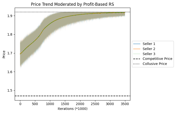
(a) Profit-Based RS

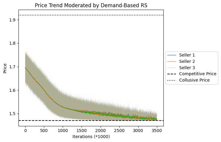
(b) Demand-Based RS

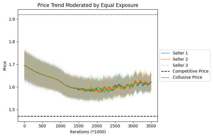
(c) Equal Exposure

Figure 1: Learning Dynamics

Note: The points on the continuous lines depict the moving average, with a window size of 1000, of the average price observed across 50 experiments at each $t$. The shaded region’s upper and lower limits indicate the highest and lowest values occurring within the window.

Table 1 also shows that after an identical number of iterations, the standard deviations of prices adhere to the following sequence: profit-based $<$ demand-based $<$ equal exposure. This finding elucidates that recommender systems can expedite the convergence of price games among sellers, particularly when the optimization objectives between the platform and the sellers are closely aligned, as in the case of profit-based recommender systems. We further present the temporal evolution of pricing structures across three distinct scenarios in Figure 1. The graphical representations of these scenarios further corroborate our findings. Specifically, sellers moderated by a profit-based recommender system exhibit a gradual and stable convergence toward the collusive price level. Conversely, sellers influenced by a demand-based recommender system tend to approach the competitive price, but with a greater degree of volatility in their pricing behavior. In the third scenario, where sellers receive equivalent exposure, the price fluctuations are observed to be more pronounced and remain unsteady after an equivalent number of periods, as in the other two cases.

The observed discrepancies originate from the recommender systems’ capability to allocate increased exposure to sellers whose pricing actions meet the objectives of the platform, while concurrently reducing exposure for those whose actions do not meet these goals. Given that sellers’ remuneration (profit) is contingent on the allocation of exposure, these sellers are induced to set a price in accordance with the platform’s objectives: namely, a collusive price for profit-based recommender systems and a competitive price for demand-based recommender systems. Besides, with the strong manipulation power of the recommendation, the evolution of price dynamics is also faster as compared to scenarios devoid of the influence of recommender systems.

Furthermore, the alignment of the objectives between the profit-based recommender system and the sellers’ goals (profit maximization) leads the sellers to adopt the platform’s preferred price without any resistance. However, a lack of congruence between the objectives of the sellers and the demand-based recommender system can impede the convergence process.

4.2 Mechanism: Punishment Strategy

In order to comprehend the intrinsic mechanism driving the pricing outcomes observed in Section 4.1, we examine the pricing strategies employed by other sellers following any deviating seller’s deviation from the equilibrium price in the presence of different recommender systems.

Previous research has consistently demonstrated that when sellers establish strategies and attain equilibrium, any deviation from the equilibrium price by a seller seeking to gain an advantage triggers other seller(s) to lower their prices in response (Wang et al. 2023, Calvano et al. 2020b). This reaction serves to penalize the deviating seller by reducing its profits and encouraging a return to the equilibrium price. However, in the presence of recommender systems, should a seller deviate from the equilibrium price, the optimal response for the other seller(s) is to maintain their current pricing. The recommender systems can then sanction and penalize the deviating seller by diminishing its exposure. Consequently, being the sole seller to establish a non-equilibrium price is no longer advantageous, and reverting to the equilibrium price becomes the preferable course of action.

To further examine such a mechanism, following Calvano et al. (2020b), the converged Q matrix is obtained, serving as a guide for the sellers in determining the actions based on the observed state. In $\text{Time}=1$, an intervention is made to exogenously compel Seller 1 to defect and set a different price, while the remaining sellers persist in employing their previously learned strategies. In the subsequent time frames, all the sellers align their actions with the converged Q matrix. As depicted in Figure 2, immediately following Seller 1’s deviation from the equilibrium price, a reversion to the equilibrium state is observed in the subsequent period. Concurrently, the remaining sellers maintain the original pricing structure because they can capitalize on the full exposure at $\text{Time}=1$ and let the recommender systems impose a punitive measure (zero exposure) on Seller 1.

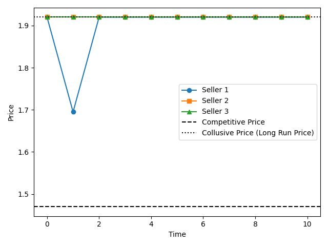
(a) Profit-Based RS

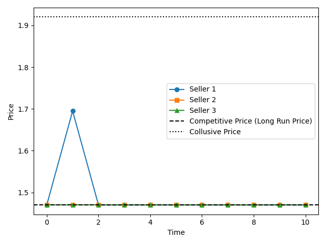
(b) Demand-Based RS

Figure 2: Deviation-Punishment Process

5 Extended Analyses

In the baseline model, following Calvano et al. (2020b), we employed the logit demand model as the economic environment, which includes a few assumptions. We relax these assumptions one by one to validate the robustness of the results. First, the baseline model assumes that the seller’s Q-learning adopts a small exploration rate, enabling long exploration to learn a more stable strategy. This assumption is adjusted in Appendix 7, where a higher exploration rate is adopted, allowing the seller to reduce exploration probability in a relatively shorter period. Second, we assumed that the platform possesses sufficient information to accurately estimate the market’s demand structure under different pricing. This assumption is relaxed in Appendix 8, where the platform is not furnished with previous knowledge of the demand structure. Lastly, in Appendix 9, we extend the economic environment to introduce customer segmentation and personalization, empowering the recommendation system to choose the best bundle for different user segments. A series of experimental results demonstrates that our conclusions are highly robust.

6 Conclusions

This study scrutinizes the influence of recommender systems on the actions of pricing algorithms and the resulting price equilibrium in e-commerce platforms. Our findings reveal that when a recommender system can allocate exposure to incentivize sellers conforming to its anticipated price and to sanction those who fail to comply, the pricing game converges expeditiously to the equilibrium that aligns with the platform’s objective. Specifically, the profit-based recommender system facilitates collusive prices, whereas the demand-based recommender system instigates competitive prices. Contrary to existing research on algorithmic collusion, the punishment mechanisms embedded within recommender systems enable an immediate rectification of sellers’ attempts to deviate from equilibrium pricing. Concurrently, non-deviating sellers do not need to alter their prevailing prices to impose penalties on those who diverge. The robustness of these findings is corroborated across a series of extensions.

Our research makes substantive contributions to various strands of literature, including the economics of artificial intelligence, recommender systems, and antitrust regulations. First, although algorithmic collusion has recently become a fervent area of inquiry (Wang et al. 2023, Dou et al. 2023, Calder-Wang and Kim 2023), existing studies have overlooked the effect of recommender systems. Given that recommender systems are extensively utilized in online marketplaces and have the ability to directly impact sellers’ profits through exposure adjustments, their role in this context is crucial. We address this gap by integrating recommender systems into the framework of the pricing game. Second, prior explorations of recommender systems predominantly regard the price as exogenous, with only a sparse number of studies modeling pricing reactions in a static manner (Zhou and Zou 2023, Li et al. 2020). However, sellers often dynamically adjust prices to maximize profits, especially as algorithmic pricing tools become more widespread. We augment this strand of literature by incorporating the dynamic reactions of sellers’ pricing algorithms, thereby examining the broader economic ramifications of recommendation systems. Last, although the literature on antitrust regulations has expressed significant concerns regarding algorithmic collusion, the debate about the precise definition and attribution of responsibility in collusion is ongoing (Robertson 2022, Colangelo 2021). Our research adds to this discourse by emphasizing the previously neglected role of platform’s recommender systems in the contemplation of regulatory measures.

Our research delineates the implications for multiple stakeholders in e-commerce platforms. For sellers and pricing algorithm designers, we emphasize that the efficacy of pricing algorithms is contingent on the platform’s recommendations. Consequently, these stakeholders must concurrently evaluate the pricing algorithms and the revenue-sharing structure with the platform, rather than considering them as isolated components. Besides, e-commerce platforms must carefully contemplate the reactions of vendors’ pricing algorithms and the consequent ramifications for social welfare when formulating recommendation algorithms. Of particular significance, the results suggest that antitrust regulation can more effectively target the platform’s recommendation algorithm, as opposed to addressing each seller separately. Finally, this study underscores the imperative need for continued investigation into algorithmic pricing and competition policy, particularly focusing on the market design and algorithms employed by intermediaries.

7 Extended Analyses with Less Exploration

In Section 4, we elucidate that the price escalates (deescalates) under conditions where the exposure is governed by profit-based (demand-based) recommender systems. In this appendix, we aim to delineate the influence of constraining the exploration capabilities of pricing algorithms on both the learning trajectory and the eventual equilibrium state.

In the Q-learning framework, the exploration rate denoted by $\omega$ modulates the likelihood of undertaking a stochastic action at each temporal interval, given by $\epsilon=e^{-\omega t}$. This probability is subject to exponential decay governed by both $\omega$ and the time parameter $t$. Prolonged exploration periods enable the algorithm to acquire a more accurate estimation of the optimal pricing strategy; however, they concurrently incur elevated opportunity costs associated with the exploration of suboptimal pricing alternatives. In our baseline configuration, $\omega$ is preset to $1.5e-6$, indicative of a relatively long exploration phase and sufficient learning of the optimal pricing. In contrast, this appendix considers a “Less Exploration” scenario, where we employ a substantially larger $\omega$ value ($5e-6$), thereby considerably curtailing the exploratory activities. For instance, after one million periods, the pricing algorithms in the baseline configuration retain an approximate likelihood of $22.31\%$ for opting for a stochastic action. Meanwhile, in the “Less Exploration” scenario, this probability is dramatically reduced to a mere $0.67\%$.

To maintain experimental consistency, we preserve all parameters identical to those in the baseline configuration, altering solely the exploration rate parameter $\omega$. The simulation is executed 50 times, with each run spanning one million periods, subsequent to which the exploration probability descends below $1\%$. The resultant average equilibrium prices and profits are tabulated in Table 1, while the temporal evolution of the learning dynamics is visually represented in Figure 3. Remarkably, the attained price equilibrium exhibits substantial congruence with the baseline scenario. Compared to the equilibrium price of 1.6515 observed in the equal-exposure condition, the implementation of profit-based recommender systems engenders an elevation in price to 1.9167. Conversely, the deployment of demand-based recommender systems yields a diminution in price to 1.4798. Additionally, the learning dynamics of the pricing algorithms, modulated by divergent types of recommender systems, advance in a smooth and monotonic manner toward their respective equilibria, aligning with the objectives of the varying recommender systems.

Table 2: Price and Profit Comparison for the Seller (Less Exploration)

	Profit-Based RS	Demand-Based RS	Equal Exposure
Prices	1.9167 (0.0039)	1.4798 (0.0057)	1.6515 (0.0151)
Profit	0.2250 (0.0042)	0.1481 (0.0050)	0.1854 (0.0041)

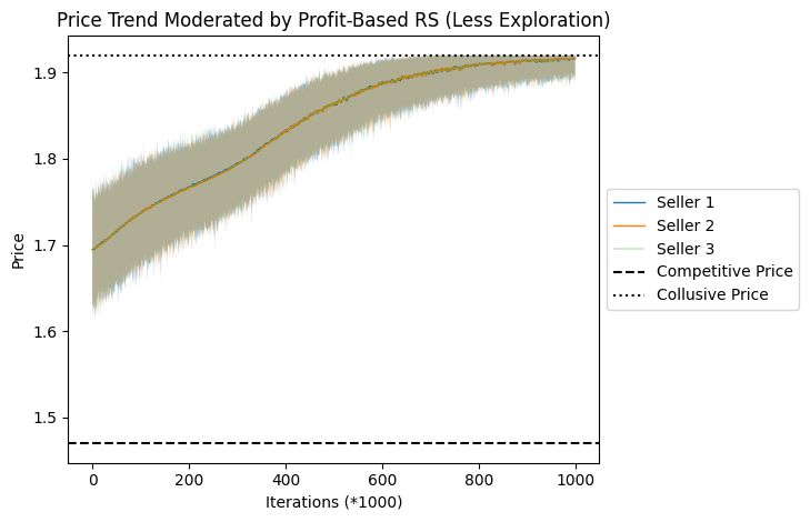
(a) Profit-Based RS

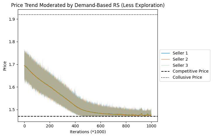
(b) Demand-Based RS

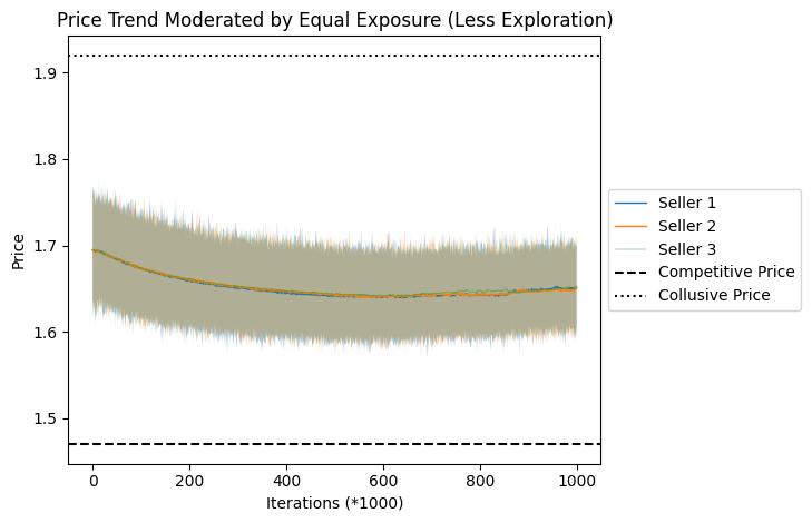
(c) Equal Exposure

Figure 3: Learning Dynamics with Less Exploration

Note: The points on the continuous lines depict the moving average, with a window size of 1000, of the average price observed across 50 experiments at each $t$. The shaded region’s upper and lower limits indicate the highest and lowest values occurring within the window.

8 Extended Analyses with Q-learning Recommender Systems

In the baseline setting, we operate under the presumption that the platform has amassed sufficient data and consequently formulated a precise model to deduce the demand for each seller as a function of pricing structures. As a result, the platform’s recommender systems can directly select the bundle of products that aligns most closely with the platform’s objectives for each time period. In the subsequent appendix, we deviate from this assumption to scrutinize a scenario wherein the platform lacks such comprehensive information and employs Q-learning methods to explore the expected rewards (total demand or profit), corresponding to various exposure allocation strategies contingent upon sellers’ pricing decisions. We update the framework and then execute simulations to assess the robustness of our findings within this extended setting.

8.1 Dynamic Pricing Competition Moderated by Q-learning RS

To conduct this analysis, we retain the economic environment and sellers’ Q-learning pricing algorithms as outlined in Section 3, albeit with modifications to the recommender systems and corresponding adjustments to the repeated game process.

8.1.1 Modification of the Recommender Systems (Q-learning RS)

In accordance with the basic framework in Section 3, the function of recommender systems is to determine the exposure allocation of each product bundle, contingent upon the pricing decisions enacted by the sellers for each time period. It is noteworthy that, in this extended analysis, the platform does not possess a priori knowledge of the underlying demand structure. To surmount this limitation, recommender systems employ a Q-learning algorithmic approach. In this context, the present period’s price vector $s^{t+1}=(p_{1}^{t},...,p_{n}^{t})$ serves as the state variable, while the exposure allocation for the entire set of bundles $x^{t}=(x_{1}^{t},...,x_{m}^{t})$ constitutes the action variable. Note that we employ $s^{t+1}$ in lieu of $s^{t}$ to maintain coherence with the state representation utilized by sellers, who incorporate the price from the preceding period as input. Subsequent to the exposure allocation, the sellers’ demand and profitability materialize. The recommender systems can then utilize either the aggregate profit $r_{t}$ or demand $d_{t}$ on the market as the reward metric depending on their categories—either profit-based or demand-based. In the ensuing period, the recommender systems update the state variable to reflect the newly established pricing vectors set forth by the sellers, denoted as $s^{t+2}=(p_{1}^{t+1},...,p_{n}^{t+1})$.

Building upon the process delineated earlier, the platform’s Q-learning-based recommender systems aim to identify the optimal Q-matrix $Q_{r}$, which possesses dimensions $|S|\times|X|$. This matrix guides the optimal exposure distribution conditional on sellers’ respective pricing strategies. At each period $t$, the recommender system assimilates both the reward metric $r^{t-1}$ (or $d^{t-1}$) and the state transition $s^{t}\rightarrow s^{t+1}$, which are consequent upon the prior exposure allocation action $x^{t-1}$. Following this observation, one element ($s^{t},x^{t-1}$) within the Q-matrix is updated in accordance with either Equation 7 for the profit-based recommender system, or Equation 8 for the demand-based one:

$$Q_{r}(s=s^{t},x=x^{t-1})=(1-\alpha)Q_{r}(s^{t},x^{t-1})+\alpha\left[r^{t-1}+\delta\max_{x\in X}Q_{r}\left(s^{t+1},x\right)\right]$$ (7)

$$Q_{r}(s=s^{t},x=x^{t-1})=(1-\alpha)Q_{r}(s^{t},x^{t-1})+\alpha\left[d^{t-1}+\delta\max_{x\in X}Q_{r}\left(s^{t+1},x\right)\right]$$ (8)

Here, we employ notation analogous to that utilized in the sellers’ Q-learning pricing algorithms. Specifically, we designate $\alpha$ as the learning rate, $\delta$ as the discount factor, and $\epsilon$ as the exploration rate. During this period, all other components of the matrix retain their extant values.

8.1.2 Modification of the Repeated Game Process (Q-learning RS)

We now elucidate the repeated game process and parameters subsequent to the incorporation of the Q-learning-based recommender systems. Specifically, our analysis remains concentrated on a triad of vendors, each vending a singular product in the marketplace.

At each period $t$, sellers operate autonomously and contemporaneously, invoking distinct Q-learning algorithms to ascertain each product $i$’s price $p_{i}^{t}$. Subsequent to this, platform’s Q-learning-based recommender system allocates exposure across all the bundles $x^{t}=(x_{1}^{t},x_{2}^{t},x_{3}^{t})$, whereupon the profit for all the sellers materialize ($r_{1}^{t}$, $r_{2}^{t}$, and $r_{3}^{t}$). Each vendor subsequently updates its Q-table $Q_{i}$, utilizing the profit as the reward $r_{i}^{t}$, the antecedent period’s prices as the pre-transitional state $s^{t}=(p_{1}^{t-1},p_{2}^{t-1},p_{3}^{t-1})$, and the contemporaneous pricing structure as the post-transitional state $s^{t+1}=(p_{1}^{t},p_{2}^{t},p_{3}^{t})$.

In addition, the platform’s recommendation algorithm ascertains its reward based on the category (profit-based or demand-based), aggregating either the total profit $r^{t}$ or total demand $d^{t}$ across all the sellers on the platform. Nonetheless, as explicated in the antecedent section, the recommender systems can only observe the state transitions influenced by the current period’s exposure allocation actions subsequent to the sellers’ pricing decisions in the next period. Given this temporal lag, in the period $t$, subsequent to all the sellers’ pricing determination $s^{t+1}$, the platform necessitates an update to its Q-table $Q_{r}$ prior to rendering its exposure allocation decision $x^{t}$.

We outline the entire dynamic game process in the pseudocode “Three Q-learning Sellers Moderated by Profit-Based Q-learning RS”, in which sellers operationalize independent algorithms denoted as $Q_{1}$, $Q_{2}$, and $Q_{3}$, while the platform leverages a Q-learning algorithm, $Q_{r}$, to optimize total profit among sellers in the market. As an alternative scenario, when the platform’s Q-learning algorithm ($Q_{r}$) is configured to optimize aggregate market demand, the corresponding process is articulated in the pseudocode“Three Q-learning Sellers Moderated by Demand-Based Q-learning RS”. Given that the main modification in this appendix pertains to the recommender system, the case of equal exposure remains invariant to the presentation in Section 4, thereby obviating the need for redundant exposition in this context.

8.1.3 Parameters (Q-learning RS)

We perpetuate all economic parameters from the baseline configuration, and preserve the parameters governing the sellers’ Q-learning algorithms with the exception of the exploration rate. This modification is necessitated by the introduction of additional stochastic elements into the environment due to the substitution of the platform’s recommender system, thereby requiring an elongated exploration phase. Accordingly, the exploration rate is adjusted to a smaller value, $\omega=1\times 10^{-7}$.

For the platform’s algorithm, the state space remains constituted by the prices of all three products, and its action space is defined by the decision to allocate exposure to three product bundles. Maintaining consistency with the notation utilized in Section 4, we denote $x_{1}^{t}$ as the exposure of the bundle comprising products 1 and 2, $x_{2}^{t}$ as the exposure of the bundle containing products 1 and 3, and $x_{3}^{t}$ as the exposure of the bundle featuring products 2 and 3 at temporal period $t$. Analogous to the sellers’ actions, we discretize the recommender system’s action space by partitioning the exposure into nine uniform segments, each bundle thereby receiving an allocation ranging from one to seven segments. For illustrative purposes, the most asymmetric exposure distribution is $x^{t}=\left(\frac{1}{9},\frac{1}{9},\frac{7}{9}\right)$, while the most equitable distribution is $x^{t}=\left(\frac{1}{3},\frac{1}{3},\frac{1}{3}\right)$. Lastly, it is imperative to note that the parameters characterizing the platform’s Q-learning-based recommender systems are harmonized to be the same as those employed by the sellers.

Three Q-learning Sellers Moderated by Profit-Based Q-learning RS

$$\text{Parameters: }\alpha_{0},\alpha_{1},\alpha_{2},\alpha_{3},c_{1},c_{2},c_{3},\mu,\alpha\in(0,1],\delta\in(0,1),\omega\in(0,\infty)$$

$$\text{Initialize }Q_{1}(s,p),Q_{2}(s,p),Q_{3}(s,p),Q_{r}(s,x)$$

$$\text{Initialize }t=1,s^{1}$$

while not converge do

$$\phantom{abcd}\epsilon\leftarrow e^{-\omega t}$$

$$\phantom{abcd}p_{i}^{t}\leftarrow\begin{cases}\arg\max_{p}Q_{i}\left(s^{t},p\right)&\text{ with probability }1-\epsilon\\ \text{a random action }&\text{ with probability }\epsilon\end{cases}\text{ for }i\in\{1,2,3\}$$

$$\phantom{abcd}s^{t+1}\leftarrow\left(p_{1}^{t},p_{2}^{t},p_{3}^{t}\right)$$

$$\phantom{abcd}Q_{r}\left(s^{t},x^{t-1}\right)\leftarrow(1-\alpha)Q_{r}\left(s^{t},x^{t-1}\right)+\alpha\left(r^{t-1}+\delta\max_{x\in X}\left(Q_{r}\left(s^{t+1},x\right)\right)\right)\text{ if }t\geq 2$$

$$\phantom{abcd}x^{t}=(x_{1}^{t},x_{2}^{t},x_{3}^{t})\leftarrow\begin{cases}\arg\max_{x}Q_{r}\left(s_{r}^{t},x\right)&\text{ with probability }1-\epsilon\\ \text{a random action }&\text{ with probability }\epsilon\end{cases}$$

$$\phantom{abcd}r_{1}^{t}\leftarrow\ (x_{1}^{t}*\frac{e^{\frac{{\alpha_{1}-p_{1}^{t}}}{\mu}}}{{e^{\frac{{\alpha_{1}-p_{1}^{t}}}{\mu}}+e^{\frac{{\alpha_{2}-p_{2}^{t}}}{\mu}}+e^{\frac{\alpha_{0}}{\mu}}}}+x_{2}^{t}*\frac{e^{\frac{{\alpha_{1}-p_{1}^{t}}}{\mu}}}{{e^{\frac{{\alpha_{1}-p_{1}^{t}}}{\mu}}+e^{\frac{{\alpha_{3}-p_{3}^{t}}}{\mu}}+e^{\frac{\alpha_{0}}{\mu}}}})*(p_{1}^{t}-c_{1})$$

$$\phantom{abcd}r_{2}^{t}\leftarrow\ (x_{1}^{t}*\frac{e^{\frac{{\alpha_{2}-p_{2}^{t}}}{\mu}}}{{e^{\frac{{\alpha_{1}-p_{1}^{t}}}{\mu}}+e^{\frac{{\alpha_{2}-p_{2}^{t}}}{\mu}}+e^{\frac{\alpha_{0}}{\mu}}}}+x_{3}^{t}*\frac{e^{\frac{{\alpha_{2}-p_{2}^{t}}}{\mu}}}{{e^{\frac{{\alpha_{2}-p_{2}^{t}}}{\mu}}+e^{\frac{{\alpha_{3}-p_{3}^{t}}}{\mu}}+e^{\frac{\alpha_{0}}{\mu}}}})*(p_{2}^{t}-c_{2})$$

$$\phantom{abcd}r_{3}^{t}\leftarrow\ (x_{2}^{t}*\frac{e^{\frac{{\alpha_{3}-p_{3}^{t}}}{\mu}}}{{e^{\frac{{\alpha_{1}-p_{1}^{t}}}{\mu}}+e^{\frac{{\alpha_{3}-p_{3}^{t}}}{\mu}}+e^{\frac{\alpha_{0}}{\mu}}}}+x_{3}^{t}*\frac{e^{\frac{{\alpha_{3}-p_{3}^{t}}}{\mu}}}{{e^{\frac{{\alpha_{2}-p_{2}^{t}}}{\mu}}+e^{\frac{{\alpha_{3}-p_{3}^{t}}}{\mu}}+e^{\frac{\alpha_{0}}{\mu}}}})*(p_{3}^{t}-c_{3})$$

$$\phantom{abcd}r^{t}\leftarrow\ r_{1}^{t}+r_{2}^{t}+r_{3}^{t}$$

$$\phantom{abcd}Q_{i}\left(s^{t},p_{i}^{t}\right)\leftarrow(1-\alpha)Q_{i}\left(s^{t},p_{i}^{t}\right)+\alpha\left(r_{i}^{t}+\delta\max_{p\in A}\left(Q_{i}\left(s^{t+1},p\right)\right)\right)\text{ for }i\in\{1,2,3\}$$

$$\phantom{abcd}t\leftarrow t+1$$

end

Three Q-learning Sellers Moderated by Demand-Based Q-learning RS

$$\text{Parameters: }\alpha_{0},\alpha_{1},\alpha_{2},\alpha_{3},c_{1},c_{2},c_{3},\mu,\alpha\in(0,1],\delta\in(0,1),\omega\in(0,\infty)$$

$$\text{Initialize }Q_{1}(s,p),Q_{2}(s,p),Q_{3}(s,p),Q_{r}(s,x)$$

$$\text{Initialize }t=1,s^{1}$$

while not converge do

$$\phantom{abcd}\epsilon\leftarrow e^{-\omega t}$$

$$\phantom{abcd}p_{i}^{t}\leftarrow\begin{cases}\arg\max_{p}Q_{i}\left(s^{t},p\right)&\text{ with probability }1-\epsilon\\ \text{a random action }&\text{ with probability }\epsilon\end{cases}\text{ for }i\in\{1,2,3\}$$

$$\phantom{abcd}s^{t+1}\leftarrow\left(p_{1}^{t},p_{2}^{t},p_{3}^{t}\right)$$

$$\phantom{abcd}Q_{r}\left(s^{t},x^{t-1}\right)\leftarrow(1-\alpha)Q_{r}\left(s^{t},x^{t-1}\right)+\alpha\left(d^{t-1}+\delta\max_{x\in X}\left(Q_{r}\left(s^{t+1},x\right)\right)\right)\text{ if }t\geq 2$$

$$\phantom{abcd}x^{t}=(x_{1}^{t},x_{2}^{t},x_{3}^{t})\leftarrow\begin{cases}\arg\max_{x}Q_{r}\left(s_{r}^{t},x\right)&\text{ with probability }1-\epsilon\\ \text{a random action }&\text{ with probability }\epsilon\end{cases}$$

$$\phantom{abcd}d_{1}^{t}\leftarrow\ x_{1}^{t}*\frac{e^{\frac{{\alpha_{1}-p_{1}^{t}}}{\mu}}}{{e^{\frac{{\alpha_{1}-p_{1}^{t}}}{\mu}}+e^{\frac{{\alpha_{2}-p_{2}^{t}}}{\mu}}+e^{\frac{\alpha_{0}}{\mu}}}}+x_{2}^{t}*\frac{e^{\frac{{\alpha_{1}-p_{1}^{t}}}{\mu}}}{{e^{\frac{{\alpha_{1}-p_{1}^{t}}}{\mu}}+e^{\frac{{\alpha_{3}-p_{3}^{t}}}{\mu}}+e^{\frac{\alpha_{0}}{\mu}}}}$$

$$\phantom{abcd}d_{2}^{t}\leftarrow\ x_{1}^{t}*\frac{e^{\frac{{\alpha_{2}-p_{2}^{t}}}{\mu}}}{{e^{\frac{{\alpha_{1}-p_{1}^{t}}}{\mu}}+e^{\frac{{\alpha_{2}-p_{2}^{t}}}{\mu}}+e^{\frac{\alpha_{0}}{\mu}}}}+x_{3}^{t}*\frac{e^{\frac{{\alpha_{2}-p_{2}^{t}}}{\mu}}}{{e^{\frac{{\alpha_{2}-p_{2}^{t}}}{\mu}}+e^{\frac{{\alpha_{3}-p_{3}^{t}}}{\mu}}+e^{\frac{\alpha_{0}}{\mu}}}}$$

$$\phantom{abcd}d_{3}^{t}\leftarrow\ x_{2}^{t}*\frac{e^{\frac{{\alpha_{3}-p_{3}^{t}}}{\mu}}}{{e^{\frac{{\alpha_{1}-p_{1}^{t}}}{\mu}}+e^{\frac{{\alpha_{3}-p_{3}^{t}}}{\mu}}+e^{\frac{\alpha_{0}}{\mu}}}}+x_{3}^{t}*\frac{e^{\frac{{\alpha_{3}-p_{3}^{t}}}{\mu}}}{{e^{\frac{{\alpha_{2}-p_{2}^{t}}}{\mu}}+e^{\frac{{\alpha_{3}-p_{3}^{t}}}{\mu}}+e^{\frac{\alpha_{0}}{\mu}}}}$$

$$\phantom{abcd}r_{i}^{t}\leftarrow\ d_{i}^{t}*(p_{i}^{t}-c_{i})\text{ for }i\in\{1,2,3\}$$

$$\phantom{abcd}d^{t}\leftarrow\ d_{1}^{t}+d_{2}^{t}+d_{3}^{t}$$

$$\phantom{abcd}Q_{i}\left(s^{t},p_{i}^{t}\right)\leftarrow(1-\alpha)Q_{i}\left(s^{t},p_{i}^{t}\right)+\alpha\left(r_{i}^{t}+\delta\max_{p\in A}\left(Q_{i}\left(s^{t+1},p\right)\right)\right)\text{ for }i\in\{1,2,3\}$$

$$\phantom{abcd}t\leftarrow t+1$$

end

8.2 Experimental Results: Q-Learning RS

Owing to the smaller exploration rate, each simulation is conducted over an extensive temporal span of 40,000,000 periods. Constrained by computational intricacies, ten simulation runs are executed, with the mean price and profit values over the terminal 10,000 periods presented in Table 3. Learning dynamics in the average pricing decisions across three sellers are visually encapsulated in Figure 4. Our findings substantiate the notion that under a profit-based platform algorithm, sellers exhibit a proclivity towards establishing supra-competitive pricing structures, exemplified by an average price of 1.8317. Conversely, in scenarios where the platform algorithm is aligned towards optimizing aggregate demand, the resultant pricing decisions manifest at considerably reduced levels, at an average of 1.5432. This observation strengthens the robustness of our conclusions, particularly in contexts where recommender systems operate with circumscribed informational inputs.

Table 3: Price and Profit Comparison for the Seller (Q-Learning RS)

	Profit-Based RS	Demand-Based RS
Prices	1.8317 (0.0259)	1.5432 (0.0283)
Profit	0.2245 (0.0195)	0.1607 (0.0162)

(a) Profit-Based RS

(b) Demand-Based RS

Figure 4: Learning Dynamics Moderated by Q-learning RS

Note: The points on the continuous lines depict the moving average, with a window size of 10,000, of the average price observed across 10 experiments at each $t$.

9 Extended Analyses with Personalized Recommender Systems

In the baseline configuration, we utilize a logit demand model devoid of customer segmentation (Calvano et al. 2020b). In this appendix, we extend the economic environment by incorporating heterogeneous customer types and subsequently adapt the recommender systems to facilitate optimization tailored to different customer categories. Notably, the core observations remain robust under this modified setting.

9.1 Dynamic Pricing Competition Moderated by Personalized RS

In this section, we initially delineate the customer segments and subsequently adapt the recommender systems to be congruent with such segmentation. The iterative game process and its associated parameters are modified commensurately.

9.1.1 Modification of the Economic Environment (Customer Segmentation)

Expanding upon the prevalent logit demand model frequently invoked in algorithmic collusion (Calvano et al. 2020b), we incorporate consumer heterogeneity by facilitating differentiated utilities for external options among various customer segments. For the sake of computational complexity and without loss of generality, we consider two distinct consumer types $T$: $H$ and $L$, endowed with respective outside option utilities $\alpha_{0,H}$ and $\alpha_{0,L}$. Furthermore, each consumer type constitutes precisely 50% of the overall consumer populace.

In alignment with Section 4, we conceptualize a marketplace featuring $n$ differentiated products, where $i$ indexes the individual products from 1 to $n$. The platform persists in recommending one out of $m$ predefined bundles (indexed by $j=1,2,\ldots,m$) to each consumer, with each bundle $j$ comprising a specific subset of products denoted as $B_{j}$. Given the existence of dual consumer types, at each temporal period $t$, the platform is necessitated to calibrate the exposure levels of each bundle $j$ for both type $T$ consumer categories, symbolized as $x_{j,T}^{t}$, subject to the constraint $\sum_{j=1}^{m}x_{j,T}^{t}=1$ for $T=L,H$. Consequently, each consumer segment $T$ in conjunction with each product bundle $j$ can be construed as constituting a distinct submarket. The demand for product $i$ emanating from the recommendation of bundle $j$ to consumers of type $T$ at period $t$ is subsequently derived as follows:

$$d_{i,j,T}^{t}=\frac{1}{2}*x_{j,T}^{t}*\frac{e^{\frac{{\alpha_{i}-p_{i}^{t}}}{\mu}}}{{\sum_{k\in B_{j}}e^{\frac{{\alpha_{k}-p_{k}^{t}}}{\mu}}+e^{\frac{\alpha_{0,T}}{\mu}}}}$$ (9)

Consequently, the demand $d_{i}^{t}$ and the associated profit $r_{i}^{t}$ for each seller $i$ at temporal period $t$ are elaborated in Equation 10 and Equation 11, respectively:

$$d_{i}^{t}=\sum_{T\in\{H,L\}}\sum_{i\in B_{j}}d_{i,j,T}^{t}$$ (10)

$$r_{i}^{t}=(p_{i}^{t}-c_{i})*d_{i}^{t}$$ (11)

9.1.2 Modification of the Recommender Systems (Personalization)

In light of customer segmentation present in this extended scenario, the platform can optimize exposure allocation conditional on disparate consumer types. Drawing upon the recommendation framework delineated in Section 4, subsequent to the sellers’ establishment of pricing decisions at each period $t$, the recommender system selects an array of most desirable bundles $B_{\text{max},T,r}^{t}$ (or $B_{\text{max},T,d}^{t}$) predicated upon the aggregated profit (or demand) for each segment $T$. The products’ exposure to this consumer segment is then equitably distributed among these selected bundles. Pseudocodes encapsulating the operational logic for profit-based and demand-based recommender systems are articulated in “Profit-Based Recommender Systems (Personalization)” and “Demand-Based Recommender Systems (Personalization)”, respectively.

Profit-Based Recommender Systems (Personalization)

$$\text{Input: }\alpha_{0,T}\text{ for }T=H,L;\alpha_{i},c_{i},p_{i}^{t}\text{ for }i=1,2,...n;B_{j}\text{ for }j=1,2,...m$$

$$\text{Initialize two lists of bundles that can cause the most profit: }B_{max,r,H}^{t},B_{max,r,L}^{t}$$

$$\text{for T}\in\{H,L\}:$$

$$\phantom{abcd}\text{ for }j\in\{1,2,...,m\}:$$

$$\phantom{abcdabcd}r_{j,T}^{t}=\sum_{i\in B_{j}}\frac{e^{\frac{{\alpha_{i}-p_{i}^{t}}}{\mu}}}{{\sum_{k\in B_{j}}e^{\frac{{\alpha_{k}-p_{k}^{t}}}{\mu}}+e^{\frac{\alpha_{0,T}}{\mu}}}}*(p_{i}^{t}-c_{i})$$

$$\text{for }j\in\{1,2,...,m\}:$$

$$\phantom{abcd}\text{ if }r_{j,H}^{t}=\max_{j^{\prime}\in\{1,2,...,m\}}r_{j,H}^{t}:$$

$$\phantom{abcdabcd}\text{Append }j\text{ to }B_{max,r,H}^{t}$$

$$\phantom{abcd}\text{ if }r_{j,L}^{t}=\max_{j^{\prime}\in\{1,2,...,m\}}r_{j,L}^{t}:$$

$$\phantom{abcdabcd}\text{Append }j\text{ to }B_{max,r,L}^{t}$$

$$\text{for }j\in\{1,2,...,m\}:$$

$$\phantom{abcd}x_{j,H}^{t}=\begin{cases}\frac{1}{|B_{max,r,H}^{t}|}&\text{ if }j\in B_{max,r,H}^{t}\\ 0&\text{otherwise}\end{cases}$$

$$\text{Output: }\{x_{1}^{t},x_{2}^{t},...,x_{m}^{t}\}$$

$$\phantom{abcd}x_{j,L}^{t}=\begin{cases}\frac{1}{|B_{max,r,L}^{t}|}&\text{ if }j\in B_{max,r,L}^{t}\\ 0&\text{otherwise}\end{cases}$$

$$\text{Output: }\{x_{1,H}^{t},x_{1,L}^{t},x_{2,H}^{t},x_{2,L}^{t},...,x_{m,H}^{t},x_{m,L}^{t},\}$$

Demand-Based Recommender Systems (Personalization)

$$\text{Input: }\alpha_{0};\alpha_{i},c_{i},p_{i}^{t}\text{ for }i=1,2,...n;B_{j}\text{ for }j=1,2,...m$$

$$\text{Initialize two lists of bundles that can cause the most demand: }B_{max,d,H}^{t},B_{max,d,L}^{t}$$

$$\text{for T}\in\{H,L\}:$$

$$\phantom{abcd}\text{ for }j\in\{1,2,...,m\}:$$

$$\phantom{abcdabcd}d_{j,T}^{t}=\sum_{i\in B_{j}}\frac{e^{\frac{{\alpha_{i}-p_{i}^{t}}}{\mu}}}{{\sum_{k\in B_{j}}e^{\frac{{\alpha_{k}-p_{k}^{t}}}{\mu}}+e^{\frac{\alpha_{0,T}}{\mu}}}}$$

$$\text{for }j\in\{1,2,...,m\}:$$

$$\phantom{abcd}\text{ if }d_{j,H}^{t}=\max_{j^{\prime}\in\{1,2,...,m\}}d_{j,H}^{t}:$$

$$\phantom{abcdabcd}\text{Append }j\text{ to }B_{max,d,H}^{t}$$

$$\phantom{abcd}\text{ if }d_{j,L}^{t}=\max_{j^{\prime}\in\{1,2,...,m\}}d_{j,L}^{t}:$$

$$\phantom{abcdabcd}\text{Append }j\text{ to }B_{max,d,L}^{t}$$

$$\text{for }j\in\{1,2,...,m\}:$$

$$\phantom{abcd}x_{j,H}^{t}=\begin{cases}\frac{1}{|B_{max,d,H}^{t}|}&\text{ if }j\in B_{max,d,H}^{t}\\ 0&\text{otherwise}\end{cases}$$

$$\text{Output: }\{x_{1}^{t},x_{2}^{t},...,x_{m}^{t}\}$$

$$\phantom{abcd}x_{j,L}^{t}=\begin{cases}\frac{1}{|B_{max,d,L}^{t}|}&\text{ if }j\in B_{max,d,L}^{t}\\ 0&\text{otherwise}\end{cases}$$

$$\text{Output: }\{x_{1,H}^{t},x_{1,L}^{t},x_{2,H}^{t},x_{2,L}^{t},...,x_{m,H}^{t},x_{m,L}^{t},\}$$

9.1.3 Modification of the Repeated Game Process (Customer Segmentation)

We still consider a triad of sellers. In each period $t$, the action of each seller $i$ remains focused on determining its product’s price $p_{i}^{t}$, thereby keeping consistent with the baseline setting. Contrarily, as delineated in Section 9.1.2, the recommender system’s output now encompasses exposure allocation targeting each consumer segments $T$, albeit the dynamically mutable input remains to be the sellers’ pricing state. As a consequence, the repeated game framework initially presented in Section 4 is hereby extended, and the game process is elaborated within the accompanying pseudocode “Three Q-learning Sellers Moderated by the Recommender Systems (Personalization)”.

9.1.4 Parameters (Customer Segmentation)

We largely maintain the economic parameters delineated in the baseline setting, encompassing the utilities attributed to the respective products ($\alpha_{1}=\alpha_{2}=\alpha_{3}=2$), their associated costs ($c_{1}=c_{2}=c_{3}=1$), and the vertical differentiation parameter ($\mu=0.25$). For the two distinct consumer types, we configure their utilities emanating from their respective outside options, denoted as $\alpha_{0,L}$ and $\alpha_{0,H}$, to be $0$ and $0.25$, respectively. Given the equilibrated $1:1$ ratio between the two types of consumers, the Bertrand-Nash equilibrium price is $1.46$, whereas the collusive price becomes $1.84$.

In terms of the parameters dictating the sellers’ Q-learning algorithm, we persist in employing the extant learning rate $\alpha=0.15$ and discount factor $\delta=0.95$. Owing to the augmented stochasticity engendered by the introduction of customer segmentation, we opt for a diminutive exploration rate $\omega=5e-7$, thereby facilitating a more comprehensive exploration. Subsequently, for the sellers’ action space, we employ these newly established collusive and competitive prices as the extremal price actions, and discretize the action space by partitioning the interval between these two prices into ten equidistant segments, thereby yielding a set of eleven feasible pricing actions.

Three Q-learning Sellers Moderated by the Recommender Systems (Personalization)

$$\text{Parameters: }\alpha_{0,L},\alpha_{0,H},\alpha_{1},\alpha_{2},\alpha_{3},c_{1},c_{2},c_{3},\mu,\alpha\in(0,1],\delta\in(0,1),\omega\in(0,\infty)$$

$$\text{Initialize }Q_{1}(s,p),Q_{2}(s,p),Q_{3}(s,p)$$

$$\text{Initialize }t=1,s^{1}$$

while not converge do

$$\phantom{abcd}\epsilon\leftarrow e^{-\omega t}$$

$$\phantom{abcd}p_{i}^{t}\leftarrow\begin{cases}\arg\max_{p}Q_{i}\left(s^{t},p\right)&\text{ with probability }1-\epsilon\\ \text{a random action }&\text{ with probability }\epsilon\end{cases}\text{ for }i\in\{1,2,3\}$$

$$\phantom{abcd}s^{t+1}\leftarrow\left(p_{1}^{t},p_{2}^{t},p_{3}^{t}\right)$$

$$\phantom{abcd}\text{Platform distributes exposure: }x^{t}=(x_{1,H}^{t},x_{1,L}^{t},x_{2,H}^{t},x_{2,L}^{t},x_{3,H}^{t},x_{3,L}^{t})$$

$$\phantom{abcd}r_{1,H}^{t}\leftarrow\ (x_{1,H}^{t}*\frac{e^{\frac{{\alpha_{1}-p_{1}^{t}}}{\mu}}}{{e^{\frac{{\alpha_{1}-p_{1}^{t}}}{\mu}}+e^{\frac{{\alpha_{2}-p_{2}^{t}}}{\mu}}+e^{\frac{\alpha_{0,H}}{\mu}}}}+x_{2,H}^{t}*\frac{e^{\frac{{\alpha_{1}-p_{1}^{t}}}{\mu}}}{{e^{\frac{{\alpha_{1}-p_{1}^{t}}}{\mu}}+e^{\frac{{\alpha_{3}-p_{3}^{t}}}{\mu}}+e^{\frac{\alpha_{0,H}}{\mu}}}})*(p_{1}^{t}-c_{1})$$

$$\phantom{abcd}r_{2,H}^{t}\leftarrow\ (x_{1,H}^{t}*\frac{e^{\frac{{\alpha_{2}-p_{2}^{t}}}{\mu}}}{{e^{\frac{{\alpha_{1}-p_{1}^{t}}}{\mu}}+e^{\frac{{\alpha_{2}-p_{2}^{t}}}{\mu}}+e^{\frac{\alpha_{0,H}}{\mu}}}}+x_{3,H}^{t}*\frac{e^{\frac{{\alpha_{2}-p_{2}^{t}}}{\mu}}}{{e^{\frac{{\alpha_{2}-p_{2}^{t}}}{\mu}}+e^{\frac{{\alpha_{3}-p_{3}^{t}}}{\mu}}+e^{\frac{\alpha_{0,H}}{\mu}}}})*(p_{2}^{t}-c_{2})$$

$$\phantom{abcd}r_{3,H}^{t}\leftarrow\ (x_{2,H}^{t}*\frac{e^{\frac{{\alpha_{3}-p_{3}^{t}}}{\mu}}}{{e^{\frac{{\alpha_{1}-p_{1}^{t}}}{\mu}}+e^{\frac{{\alpha_{3}-p_{3}^{t}}}{\mu}}+e^{\frac{\alpha_{0,H}}{\mu}}}}+x_{3,H}^{t}*\frac{e^{\frac{{\alpha_{3}-p_{3}^{t}}}{\mu}}}{{e^{\frac{{\alpha_{2}-p_{2}^{t}}}{\mu}}+e^{\frac{{\alpha_{3}-p_{3}^{t}}}{\mu}}+e^{\frac{\alpha_{0,H}}{\mu}}}})*(p_{3}^{t}-c_{3})$$

$$\phantom{abcd}r_{1,L}^{t}\leftarrow\ (x_{1,L}^{t}*\frac{e^{\frac{{\alpha_{1}-p_{1}^{t}}}{\mu}}}{{e^{\frac{{\alpha_{1}-p_{1}^{t}}}{\mu}}+e^{\frac{{\alpha_{2}-p_{2}^{t}}}{\mu}}+e^{\frac{\alpha_{0,L}}{\mu}}}}+x_{2,L}^{t}*\frac{e^{\frac{{\alpha_{1}-p_{1}^{t}}}{\mu}}}{{e^{\frac{{\alpha_{1}-p_{1}^{t}}}{\mu}}+e^{\frac{{\alpha_{3}-p_{3}^{t}}}{\mu}}+e^{\frac{\alpha_{0,L}}{\mu}}}})*(p_{1}^{t}-c_{1})$$

$$\phantom{abcd}r_{2,L}^{t}\leftarrow\ (x_{1,L}^{t}*\frac{e^{\frac{{\alpha_{2}-p_{2}^{t}}}{\mu}}}{{e^{\frac{{\alpha_{1}-p_{1}^{t}}}{\mu}}+e^{\frac{{\alpha_{2}-p_{2}^{t}}}{\mu}}+e^{\frac{\alpha_{0,L}}{\mu}}}}+x_{3,L}^{t}*\frac{e^{\frac{{\alpha_{2}-p_{2}^{t}}}{\mu}}}{{e^{\frac{{\alpha_{2}-p_{2}^{t}}}{\mu}}+e^{\frac{{\alpha_{3}-p_{3}^{t}}}{\mu}}+e^{\frac{\alpha_{0,L}}{\mu}}}})*(p_{2}^{t}-c_{2})$$

$$\phantom{abcd}r_{3,L}^{t}\leftarrow\ (x_{2,L}^{t}*\frac{e^{\frac{{\alpha_{3}-p_{3}^{t}}}{\mu}}}{{e^{\frac{{\alpha_{1}-p_{1}^{t}}}{\mu}}+e^{\frac{{\alpha_{3}-p_{3}^{t}}}{\mu}}+e^{\frac{\alpha_{0,L}}{\mu}}}}+x_{3,L}^{t}*\frac{e^{\frac{{\alpha_{3}-p_{3}^{t}}}{\mu}}}{{e^{\frac{{\alpha_{2}-p_{2}^{t}}}{\mu}}+e^{\frac{{\alpha_{3}-p_{3}^{t}}}{\mu}}+e^{\frac{\alpha_{0,L}}{\mu}}}})*(p_{3}^{t}-c_{3})$$

$$\phantom{abcd}r_{i}^{t}\leftarrow r_{i,H}^{t}+r_{i,L}^{t}\text{ for }i\in\{1,2,3\}$$

$$\phantom{abcd}Q_{i}\left(s^{t},p_{i}^{t}\right)\leftarrow(1-\alpha)Q_{i}\left(s^{t},p_{i}^{t}\right)+\alpha\left(r_{i}^{t}+\delta\max_{p\in A}\left(Q_{i}\left(s^{t+1},p\right)\right)\right)\text{ for }i\in\{1,2,3\}$$

$$\phantom{abcd}t\leftarrow t+1$$

end

9.2 Experimental Results: Customer Segmentation and Personalization

Congruence with prior settings, each simulation extends for a duration of $8,000,000$ periods, subsequent to which the exploration probability is reduced to below $1\%$. We undertake 30 distinct simulation runs and tabulate the arithmetic mean of the price and profit metrics pertaining to Seller 1 during the concluding $1,000$ periods, as delineated in Table 4. The learning dynamics manifesting in the average pricing decisions across the triad of sellers are visually synthesized in Figure 5.

As shown in Table 4, when the platform adopts a profit-based recommendation algorithm, vendors demonstrate a proclivity for adopting elevated pricing strategies, as evidenced by an average price of $1.7893$, in contrast to an average of $1.5615$ under equal-exposure conditions. Conversely, when the platform’s recommendation system is geared towards the optimization of aggregate demand, a more competitive pricing strategy is adopted, yielding an average price of $1.4772$. As depicted in Figure 5, vendors’ pricing decisions exhibit rapid and monotonic convergence to the equilibrium price under the aegis of recommendation systems. Notably, increased price volatility is observed when the objectives of the (demand-based) recommendation system diverge from those of the vendors, or when exposure optimization is absent. These findings corroborate our primary results, thereby reinforcing the robustness of our conclusions in scenarios incorporating customer segmentation and personalized recommendation algorithms.

Table 4: Price and Profit Comparison for the Seller (Customer Segmentation)

	Profit-Based RS	Demand-Based RS	Equal Exposure
Prices	1.7893 (0.0078)	1.4772 (0.0106)	1.5615 (0.0136)
Profit	0.1921 (0.0065)	0.1403 (0.0076)	0.1577 (0.0029)

(a) Profit-Based RS (Personalization)

(b) Demand-Based RS (Personalization)

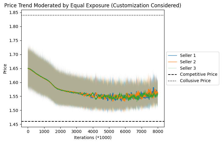
(c) Equal Exposure

Figure 5: Learning Dynamics with Customer Segmentation

Note: The points on the continuous lines depict the moving average, with a window size of 1000, of the average price observed across 30 experiments at each $t$. The shaded region’s upper and lower limits indicate the highest and lowest values occurring within the window.

References

- Abada and Lambin (2023) Abada I, Lambin X (2023) Artificial intelligence: Can seemingly collusive outcomes be avoided? Management Science .
- Agrawal et al. (2019) Agrawal A, Gans J, Goldfarb A (2019) The economics of artificial intelligence: an agenda (University of Chicago Press).
- Assad et al. (2020) Assad S, Clark R, Ershov D, Xu L (2020) Algorithmic pricing and competition: Empirical evidence from the german retail gasoline market .
- Banchio and Skrzypacz (2022) Banchio M, Skrzypacz A (2022) Artificial intelligence and auction design. Proceedings of the 23rd ACM Conference on Economics and Computation, 30–31.
- Calder-Wang and Kim (2023) Calder-Wang S, Kim GH (2023) Coordinated vs efficient prices: The impact of algorithmic pricing on multifamily rental markets. Available at SSRN 4403058 .
- Calvano et al. (2020a) Calvano E, Calzolari G, Denicolò V, Harrington Jr JE, Pastorello S (2020a) Protecting consumers from collusive prices due to ai. Science 370(6520):1040–1042.
- Calvano et al. (2019) Calvano E, Calzolari G, Denicolò V, Pastorello S (2019) Algorithmic pricing what implications for competition policy? Review of industrial organization 55:155–171.
- Calvano et al. (2020b) Calvano E, Calzolari G, Denicolo V, Pastorello S (2020b) Artificial intelligence, algorithmic pricing, and collusion. American Economic Review 110(10):3267–3297.
- Chen et al. (2008) Chen LS, Hsu FH, Chen MC, Hsu YC (2008) Developing recommender systems with the consideration of product profitability for sellers. Information sciences 178(4):1032–1048.
- Colangelo (2021) Colangelo G (2021) Artificial intelligence and anticompetitive collusion: From the ‘meeting of minds’ towards the ‘meeting of algorithms’? TTLF Stanford Law School Working Paper .
- Colliard et al. (2022) Colliard JE, Foucault T, Lovo S (2022) Algorithmic pricing and liquidity in securities markets. HEC Paris Research Paper .
- Dou et al. (2023) Dou WW, Goldstein I, Ji Y (2023) Ai-powered trading, algorithmic collusion, and price efficiency. Available at SSRN 4452704 .
- Duan et al. (2008) Duan W, Gu B, Whinston AB (2008) The dynamics of online word-of-mouth and product sales—an empirical investigation of the movie industry. Journal of retailing 84(2):233–242.
- Edelman and Wright (2015) Edelman B, Wright J (2015) Price coherence and excessive intermediation. The Quarterly Journal of Economics 130(3):1283–1328.
- Evans (2003) Evans DS (2003) The antitrust economics of multi-sided platform markets. Yale J. on Reg. 20:325.
- Fzrachi and Stucke (2019) Fzrachi A, Stucke ME (2019) Sustainable and unchallenged algorithmic tacit collusion. Nw. J. Tech. & Intell. Prop. 17:217.
- Hansen et al. (2021) Hansen KT, Misra K, Pai MM (2021) Frontiers: Algorithmic collusion: Supra-competitive prices via independent algorithms. Marketing Science 40(1):1–12.
- Harrington (2018) Harrington JE (2018) Developing competition law for collusion by autonomous artificial agents. Journal of Competition Law & Economics 14(3):331–363.
- Kang and McAuley (2018) Kang WC, McAuley J (2018) Self-attentive sequential recommendation. 2018 IEEE international conference on data mining (ICDM), 197–206 (IEEE).
- Klein (2021) Klein T (2021) Autonomous algorithmic collusion: Q-learning under sequential pricing. The RAND Journal of Economics 52(3):538–558.
- Li et al. (2020) Li L, Chen J, Raghunathan S (2020) Informative role of recommender systems in electronic marketplaces: A boon or a bane for competing sellers. MIS Quarterly 44(4).
- Mnih et al. (2015) Mnih V, Kavukcuoglu K, Silver D, Rusu AA, Veness J, Bellemare MG, Graves A, Riedmiller M, Fidjeland AK, Ostrovski G, et al. (2015) Human-level control through deep reinforcement learning. nature 518(7540):529–533.
- Parker et al. (2020) Parker G, Petropoulos G, Van Alstyne MW (2020) Digital platforms and antitrust .
- Robertson (2022) Robertson VH (2022) Antitrust law and digital markets: a guide to the european competition law experience in the digital economy .
- Salcedo (2015) Salcedo B (2015) Pricing algorithms and tacit collusion. Manuscript, Pennsylvania State University .
- Schwalbe (2018) Schwalbe U (2018) Algorithms, machine learning, and collusion. Journal of Competition Law & Economics 14(4):568–607.
- Silver et al. (2016) Silver D, Huang A, Maddison CJ, Guez A, Sifre L, Van Den Driessche G, Schrittwieser J, Antonoglou I, Panneershelvam V, Lanctot M, et al. (2016) Mastering the game of go with deep neural networks and tree search. nature 529(7587):484–489.
- Tan and Zhou (2021) Tan G, Zhou J (2021) The effects of competition and entry in multi-sided markets. The Review of Economic Studies 88(2):1002–1030.
- Van Hasselt et al. (2016) Van Hasselt H, Guez A, Silver D (2016) Deep reinforcement learning with double q-learning. Proceedings of the AAAI conference on artificial intelligence, volume 30.
- Waltman and Kaymak (2008) Waltman L, Kaymak U (2008) Q-learning agents in a cournot oligopoly model. Journal of Economic Dynamics and Control 32(10):3275–3293.
- Wang et al. (2023) Wang Q, Huang Y, Singh PV, Srinivasan K (2023) Algorithms, artificial intelligence and simple rule based pricing. Available at SSRN 4144905 .
- Watkins (1989) Watkins CJCH (1989) Learning from delayed rewards .
- Wieting and Sapi (2021) Wieting M, Sapi G (2021) Algorithms in the marketplace: An empirical analysis of automated pricing in e-commerce. Available at SSRN 3945137 .
- Zhang et al. (2019) Zhang S, Yao L, Sun A, Tay Y (2019) Deep learning based recommender system: A survey and new perspectives. ACM computing surveys (CSUR) 52(1):1–38.
- Zhou and Zou (2023) Zhou B, Zou T (2023) Competing for recommendations: The strategic impact of personalized product recommendations in online marketplaces. Marketing Science 42(2):360–376.