Fall Prediction for Bipedal Robots: The Standing Phase

Abstract

This paper presents a novel approach to fall prediction for bipedal robots, specifically targeting the detection of potential falls while standing caused by abrupt, incipient, and intermittent faults. Leveraging a 1D convolutional neural network (CNN), our method aims to maximize lead time for fall prediction while minimizing false positive rates. The proposed algorithm uniquely integrates the detection of various fault types and estimates the lead time for potential falls. Our contributions include the development of an algorithm capable of detecting abrupt, incipient, and intermittent faults in full-sized robots, its implementation using both simulation and hardware data for a humanoid robot, and a method for estimating lead time. Evaluation metrics, including false positive rate, lead time, and response time, demonstrate the efficacy of our approach. Particularly, our model achieves impressive lead times and response times across different fault scenarios with a false positive rate of 0. The findings of this study hold significant implications for enhancing the safety and reliability of bipedal robotic systems.

I Introduction

The distinct morphology of bipedal robots endows them with the unique capability to navigate diverse terrains, from unstructured environments to human-centric spaces, making them ideal candidates for assisting in daily tasks and critical situations. Nevertheless, the real-world deployment of bipedal robots remains limited. Their high-dimensional, hybrid nature, combined with occasional stringent constraints, complicates the achievement of stable motion, particularly when confronted with disturbances.

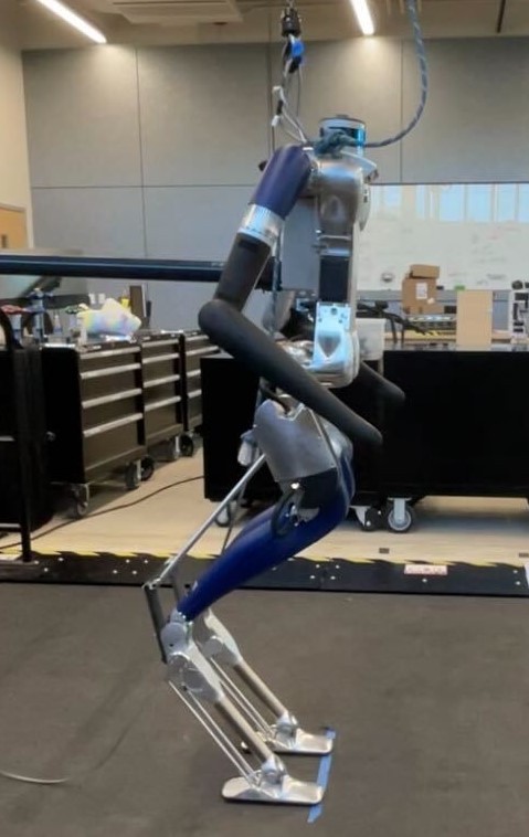
Figure 1: The experimental setup that was used to collect hardware data with the Digit robot [1].

I-A Motivation

Although a well-designed controller can counteract certain disturbances, it is infeasible to anticipate every potential disruption a bipedal robot might face in real-world scenarios. This unpredictability underscores the inevitability of falls. To truly harness the capabilities of bipedal robots, there is a pressing need for fall prediction algorithms that can foresee a fall with ample lead time, where lead time denotes the interval between the fall prediction and its actual occurrence. Addressing this need, our paper presents a 1D convolutional neural network-based fall prediction algorithm. This algorithm not only predicts falls but also estimates the lead time, specifically for the standing task with the Digit bipedal robot [1]. We focus on the standing task as it offers a simplified context for fall prediction while laying the groundwork for more dynamic movements.

I-B Background

Falls in bipedal robots can often be traced back to faults, which are characterized as unforeseen deviations in one or more operational variables. Based on their temporal behavior, faults can be classified into three categories: abrupt, incipient, and intermittent. Abrupt faults manifest as sudden or rapid changes, incipient faults evolve gradually over time, and intermittent faults appear sporadically [2]. Each of these fault types can arise during real-world operations. For example, abrupt faults might be triggered by unexpected interactions with the environment (e.g., stepping in a hole), incipient faults could stem from discrepancies in the model (e.g., poor trajectory tracking in the operational space of the robot), and intermittent faults might emerge in unpredictable environments laden with obstacles. In this context, we term the faults that precipitate a fall as critical fault and the paths leading to a fall as unsafe trajectories.

I-C Literature Review

Existing fall prediction algorithms for bipedal robots predominantly target the detection of critical abrupt faults. The primary method consists of establishing a threshold that distinguishes these faults from regular data. Selecting a threshold is a delicate task due to the impracticality of accounting for every potential critical fault and the complexity of capturing (e.g., in a model) all the robot’s safe states. Additionally, the presence of faulty states in the data is infrequent.

The overarching aim of fall prediction algorithms is to extend the lead time while curtailing the false positive rate. Consequently, their performance is typically assessed based on these two metrics [3]. On the one hand, it’s important to note that there’s an inherent positive correlation between lead time and false positive rate. On the other hand, the impact of false negatives can be alleviated by setting thresholds on kinematic signals, such as the height of the center of mass, as elaborated in [4]. The minimum lead time deemed acceptable varies depending on the specific robot and the selected recovery algorithm.

In the realm of fall prediction, thresholds are derived from various sources: analytical models like [5, 6, 7, 8, 9], hand-crafted features as seen in [10, 11, 12, 13, 14], or data-driven models such as [4, 15, 16, 17, 18, 19, 20, 5, 21, 22]. While analytical models offer a structured approach, they can be hampered by model uncertainties and might not fully encapsulate the robot’s full dynamics, especially if based on simplifying assumptions. Simple thresholds are elusive for multifaceted systems like bipedal robots. On the other hand, while data-driven models might necessitate extensive data and remain constrained to the data’s distribution, their popularity is on the rise, thanks to advancements in machine learning and computational capabilities. Both shallow methods [4, 15, 16, 17, 18, 19, 20] and deeper neural network-based approaches [21, 22] have found their place in the literature.

I-D Objective of the Paper

Our goals are as follows:

1. Detect imminent falls caused by abrupt, incipient, and intermittent faults, ensuring an adequate lead time for the standing task.

2. Optimize the trade-off between maximizing lead time and minimizing false positive rates.

3. Accurately estimate the lead time.

A robot is deemed to have fallen if the height of its center of mass descends below 0.12m. Drawing parallels with our prior research [23], we adopt 0.2s as the minimum desired lead time, aligning with the requirements of reflexive algorithms such as those in [24, 15]. Achieving this objective presents challenges, given the controller’s masking effects, the crowding phenomenon induced by incipient faults [25], the direct correlation between false positive rates and lead time, the sporadic nature of intermittent faults, and the diminishing number of data points with increasing lead time.

To address these challenges, we propose a 1D convolutional neural network (CNN)-driven fall prediction algorithm, enhanced with several components. Our choice of a deep model is motivated by the significant impact of user-selected features on lead time and false positive rates, as evidenced in our earlier work [23]. Furthermore, extracting these features for complicated bipedal robots, like Digit, is non-trivial. Our choice of a 1D CNN is underpinned by its translational equivariance and proficiency in discerning local patterns in data with a grid structure. It is noteworthy that a bipedal robot’s trajectory can be mapped onto a 1D grid, sampled at consistent (uniform) intervals [26].

I-E Contributions

We present several key contributions in this work:

• Introduction of an algorithm capable of detecting abrupt, incipient, and intermittent faults in full-sized robots undertaking a standing task.

• Successful implementation of our fall prediction algorithm, both in simulation and on hardware, tailored for a full-sized humanoid robot.

• Development of a robust method to estimate lead time.

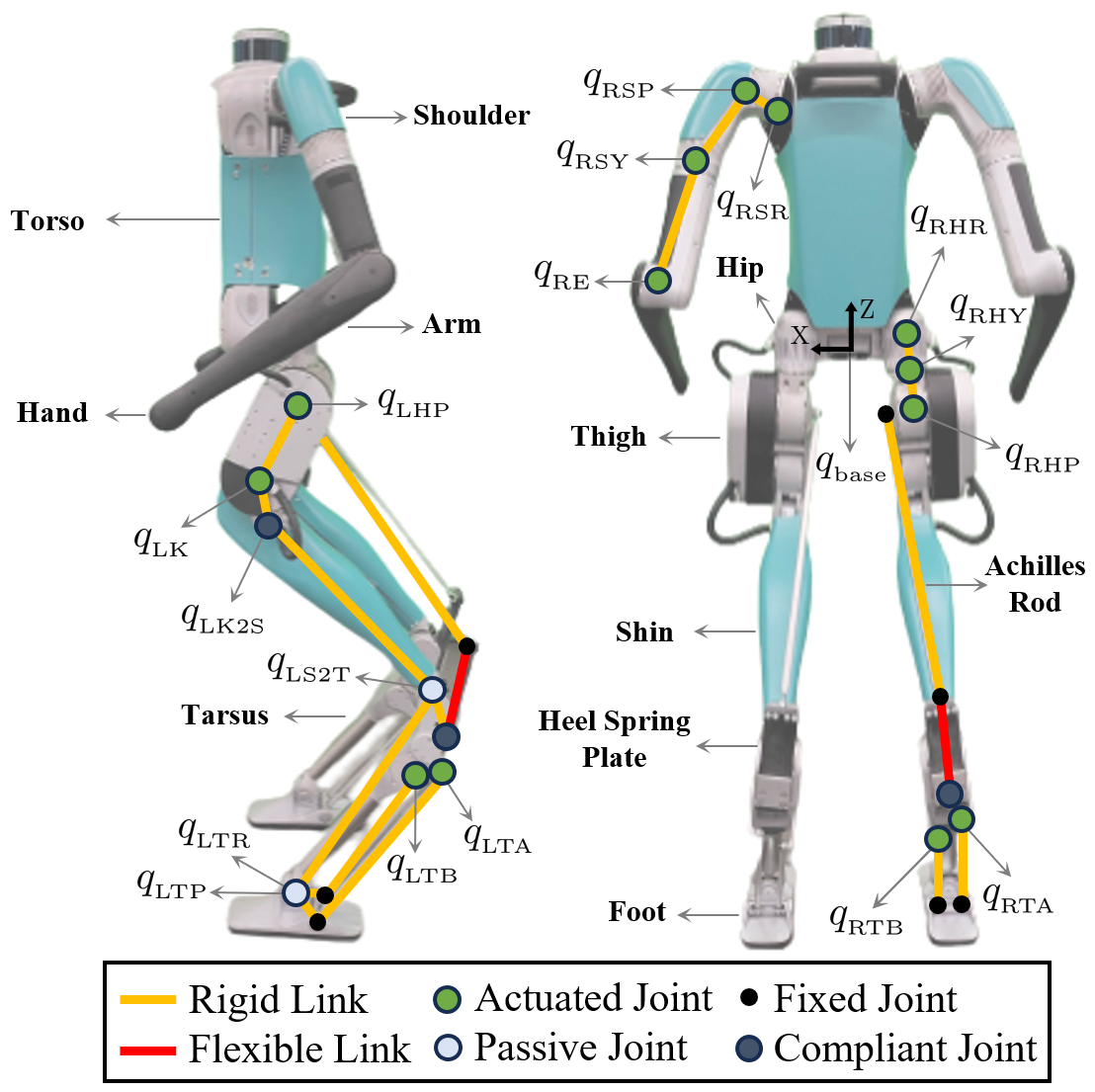
Figure 2: Kinematics architecture of the Digit robot by Agility Robotics [1]. Image Credit: Grant Gibson [27].

II Hardware Overview and Data Generation

This section provides an overview of the bipedal robot, Digit, and outlines our approach to data generation.

II-A Hardware Overview

Developed by Agility Robotics, Digit is a state-of-the-art bipedal robot [1]. While it draws inspiration from Agility Robotic’s earlier model, Cassie, Digit distinguishes itself with the addition of a torso and an integrated perception system. Possessing 30 degrees of freedom, Digit has 20 actuated joints. Weighing in at 48kg, its lower limb design is inspired by a Cassowary bird, leading to the unique nomenclature where what would typically be termed “feet” are actually “toes”; we will use the latter terminology. The kinematic architecture of Digit is illustrated in Figure 2.

II-B Simulation Data Generation

We employ Agility’s MuJoCo-based simulator in conjunction with a standing controller. This controller is designed with the primary objective of maintaining both the center of mass and the zero moment point within the support polygon [27]. We generate 900 trajectories each for abrupt and incipient faults, and 100 trajectories for intermittent faults. These faults are simulated by applying forces of various magnitudes to the robot’s torso in the $x$-direction (i.e., sagittal plane).

Abrupt faults are simulated using impulsive forces with a duration of 0.075s, randomly uniformly distributed within a range of 0 - 414.8N. In the case of incipient faults, their crowding effect is captured through trapezoidal force profiles [28] as depicted in Figure 3. These profiles have a slope of $\frac{480N}{s}$ over a varying duration to result in a desired constant amplitude over a time duration of 1s; the resulting force amplitudes of incipient faults are randomly uniformly distributed between 0 - 57.6N. The force ranges for both abrupt and incipient faults are calibrated to ensure an equal distribution of falling and safe trajectories. Emulating the unpredictable nature of intermittent faults, we apply two distinct forces. These forces are designed to mimic either abrupt or intermittent faults. The time between the introduction of the forces is randomized between 1 - 2.5s. The first force’s magnitude remains within the safe range, while the second force’s magnitude can potentially lead to a fall or maintain stability.

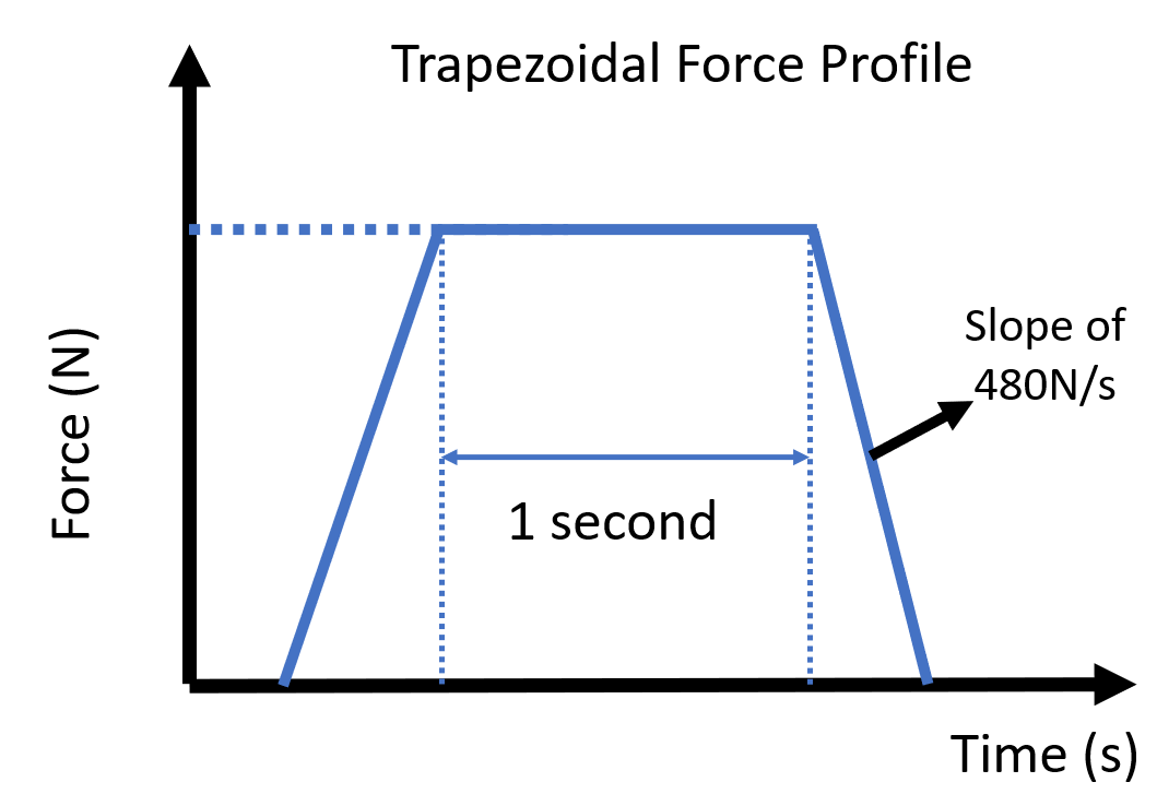
Figure 3: The trapezoidal force profile that is used to introduce incipient faults.

To simulate minor disturbances that might induce slight oscillations in the robot’s standing posture, we introduce impulsive forces with a 0.075s duration, ranging from 0 - 202.4N, at the start of each trajectory. However, only data recorded one second after the introduction of this perturbative force is retained. The abrupt and incipient faults are subsequently introduced between 2 - 2.5s following this oscillatory perturbation.

II-C Hardware Data Generation

To prevent the Digit robot from getting damaged during data collection, the hardware data generation is carried out with Digit attached to a gantry. Additionally, the motor power is “killed” when the robot starts to fall, thereby allowing the gantry to catch it. Note that we attempt to “kill” the motors prior to the gantry catching the robot. Impulsive and trapezoidal forces are introduced to the robot’s torso by pushing Digit with a pole. To emulate the trapezoidal forces that result in an incipient fault, the pole is first rested on Digit before pushing. Twenty-seven (27) safe and 13 unsafe trajectories are collected for abrupt faults, while 26 safe and 15 unsafe trajectories are collected for incipient faults. Out of the abrupt and incipient unsafe trajectories, 6 and 10, respectively, exhibited trajectory profiles resembling those observed in simulations characterized by lower falling forces. The remaining falling trajectories exhibited similarities to simulation profiles featuring forces within the mid-range of the falling forces. Figure 1 depicts the experimental setup of the hardware data.

II-D Data Pre-processing

From the 1,800 simulation-generated trajectories for abrupt and incipient faults, 200 are reserved for testing. The remaining trajectories are divided into training (80%) and validation sets. The testing set is further supplemented with intermittent fault data and hardware data. We employ Scikit-learn’s stratified train-test split method for segmenting the simulation data and its min-max scaler to normalize the data within the range ${0,1}$. It’s important to note that only transient data is utilized during training. To adjust for any drift in the hardware data, the initial feature values are subtracted from subsequent data points. Lastly, sliding windows are utilized so as to prioritize the most recent data points.

III Fall Prediction Method

The task of detecting critical faults and estimating lead time can be framed as a regression problem where lead time serves as the predicted variable. Given our definitions of lead time and critical faults, data points from unsafe trajectories prior to a critical fault’s onset, along with all data points from safe trajectories, are assigned an infinite lead time. Data points following the introduction of a critical fault have a lead time within the range $[0,H]$, where $H>0$ represents the maximum prediction horizon (i.e, maximum interval of time over which fault prediction is attempted). Predicting a lead time less than $H$ can thus indicate the presence of critical faults. However, as illustrated in Figure 4, the quantity of data points diminishes exponentially with increasing lead time, leading to an imbalanced regression challenge.

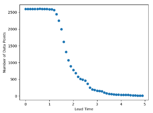
Figure 4: The number of data points vs. lead time.

While techniques like the Synthetic Minority Over-Sampling Technique for Regression with Gaussian Noise [29] exist for addressing imbalanced regression data, the direct correlation between lead time and false positive rate complicates achieving maximum lead time with an acceptable false positive rate, as evidenced by studies like [4, 22]. Consequently, we reframe the problem into a combined classification and regression challenge. Our proposed algorithm consists of three main components: a critical fault classifier, a lead time classifier, and a lead time regressor. All three components share a 1D CNN architecture, featuring a 1D CNN layer, a max pooling layer, and two fully connected layers with the ReLu activation function. The 1D CNN architecture is depicted in Figure 5.

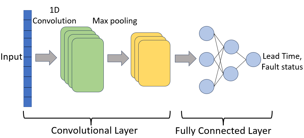
Figure 5: 1D CNN architecture of the fault detection network. It consists of a single CNN layer with a max pooling layer followed by 2 fully connected layers.

The critical fault classifier’s objective is to predict critical faults while maximizing lead time and minimizing false positives. The lead time classifier, on the other hand, categorizes windows containing critical faults into three distinct ranges: $(0,1]$, $(1,2]$, and $(2,H]$. Notably, the $(2,H]$ range contains significantly fewer data points, as shown in Figure 4. Finally, the lead time regressor predicts the lead time for windows that have a critical fault and a lead time within the range $(0,1]$.

The components of the algorithm interact sequentially. Initially, the critical fault classifier processes a window of data points from the robot. If a critical fault is detected, this window is then relayed to the lead time classifier, which categorizes the window based on the predefined lead time intervals. If the categorized lead time is within the $(0,1]$ interval, the lead time regressor determines the exact predicted lead time. For other intervals, the minimum lead time corresponding to that interval is reported (e.g, 1 for the interval $[1,2)$). The entire workflow of the proposed fall prediction algorithm is depicted in Figure 6.

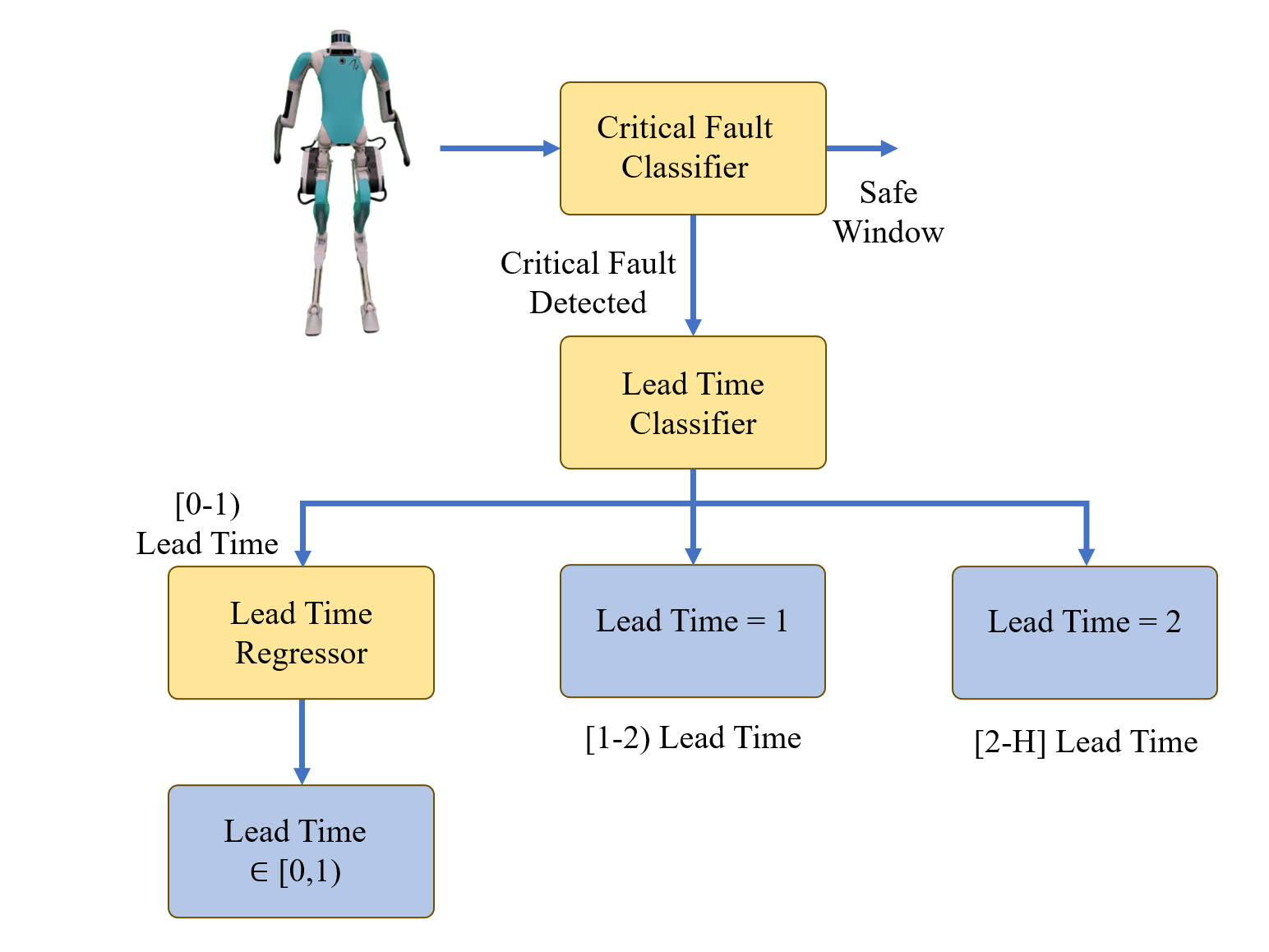
Figure 6: The proposed fall prediction algorithm with three components: critical fault classifier, lead time classifier and lead time regressor. The blue boxes depict the output of the entire algorithm.

IV Critical Fault Classifier

The features for the critical fault classifier are defined as,

$$\begin{bmatrix}(p_{com}-p_{midtoe})^{xz}\\ v_{com}^{xz}\\ q_{\text{sag chosen}}\\ \dot{q}_{\text{sag chosen}}\end{bmatrix}$$ (1)

where $p_{com}$, $v_{com}$, and $p_{midtoe}$ represent the position and velocity of the center of mass and the midpoint of the two toes, respectively. The terms $q_{\text{sag chosen}}$ and $\dot{q}_{\text{sag chosen}}$ denote the torso, knee, hip, and toe pitch angles (in the sagittal plane).

The data for abrupt and incipient faults are structured as,

$$\hskip 99.58464ptD=\{X_{i},y_{i}\}_{i=1}^{n},$$

where

$$\begin{array}[]{rcl}n&=&\text{number of windows across all training data}\\ m&=&\text{number of time steps in a window}\\ x_{ij}&=&\text{features at time step j in window i}\\ t_{i}&=&\text{time at time step i}\\ t_{\text{ft}}&=&\text{time the fault is introduced}\\ \mathbf{T}_{safe}&=&\text{safe trajectories}\\ \mathbf{T}_{unsafe}&=&\text{unsafe trajectories}\\ X_{i}&=&\begin{bmatrix}x_{i1}&&x_{i2}&&\cdots&&x_{im}\end{bmatrix}^{\intercal}\\ \\ y_{i}&\in&\ \begin{cases}1&\quad\left(X_{i}~{}\in~{}\mathbf{T}_{unsafe}\land~{}t_{i}~{}\geq~{}t_{\text{ft}}\right)\\ \\ 0&\quad\left(\begin{array}[]{cc}X_{i}~{}\in~{}\mathbf{T}_{safe}\\ \lor\\ (X_{i}~{}\in~{}\mathbf{T}_{unsafe}\land~{}t_{i}~{}<~{}t_{\text{ft}})\end{array}\right).\end{cases}\end{array}$$

With the above labeling, achieving correct identification for all windows would yield the maximum possible lead time. For intermittent data, the labeling approach remains similar, but $t_{\text{ft}}$ is the time of the first fault’s introduction.

The binary cross-entropy loss is employed for training. The classifier’s output, when combined with this loss, produces logits. These logits can be transformed into probabilities using the sigmoid function, allowing for flexibility in setting the desired probability threshold for critical fault detection. For instance, a model with a 0.03 false positive rate and a 1.7s lead time for abrupt and incipient faults can achieve a 0 false positive rate with a 1.61s lead time by adjusting the probability threshold from 0.5 to 0.9.

To optimize lead time and minimize false positive rates, the model’s performance is evaluated at each epoch. A model is saved only if it meets one of the following criteria:

1. A reduction in the false positive rate of validation trajectories.

2. No change in the validation false positive rate, but an increase in validation lead time, accompanied by a decrease in the training data’s false positive rate.

3. Both the validation and training false positive rates meet a predefined maximum threshold.

It’s worth noting that the false positive rates used in the saving criteria pertain to entire trajectories, not individual windows.

IV-A Training

We train on a subset of abrupt and incipient simulation trajectories as described in Section II-D. We use false positive rate, lead, and response time as our evaluation criteria. Response time is defined as the difference in time between the detection of the critical fault and its introduction. Given that the robot was not allowed to fall to the ground during hardware data collection, lead time is not defined for hardware. Similarly, given that intermittent data has 2 disturbances, it is difficult to estimate the response time.

IV-B Results

We evaluate on hardware trajectories, as well as on the intermittent and remaining incipient and abrupt trajectories, as defined in Section II-D. The critical fault classifier is able to achieve 0 false positive rate for training and validation data when trained for 4 epochs with 8 filters for the 1D CNN. When evaluated on testing data, the model is able to achieve 0 false positive and negative rates for hardware, intermittent, abrupt, and incipient fault data.

The resulting average lead times are 1.64s and 1.61s for intermittent and abrupt plus incipient data, respectively. The classifier’s success in categorizing the intermittent data can be attributed to the sliding window formulation, which allows the algorithm to recognize local patterns. The resulting response time is 0.39s and 0.4s for the abrupt and incipient simulation data, and hardware data, respectively. Given that the critical fault classifier detects incipient, abrupt, and intermittent faults with a lead time greater than 0.2s, it meets our objective of detecting critical faults with sufficient lead time. The results are summarized in Table I.

TABLE I: Results of the critical fault classifier when trained on abrupt and incipient simulation data and evaluated on (a) abrupt and incipient simulation data, (b) abrupt and incipient hardware data, and (c) intermittent data. Trained for 4 epochs with 8 filters.

Platform	Fault Type	Lead Time (s)	Response Time (s)	False Positive Rate
Simulation	Intermittent	1.64	N/A	0.0
Simulation	Abrupt and Incipient	1.61	0.39	0.0
Hardware	Abrupt and Incipient	N/A	0.4	0.0

V Lead Time Prediction

While the hardware data lacks a defined lead time, the similarity in response time between the hardware and simulation data, as indicated in I, suggests that the hardware may have a lead time comparable to that of the simulation data. Nevertheless, there is a critical need for lead time prediction.

Given the absence of a defined lead time for the hardware data, this section evaluates the lead time algorithms using only simulation data. The subsequent section will apply the complete fall prediction algorithm to both hardware and simulation datasets.

The feature set for lead time prediction includes those from (1), complemented by the hip, knee, and toe pitch torques, as well as the average position of the contact point.

V-A Lead Time Classifier

In this section, we detail our approach to categorizing lead times for potential falls. The categorization of lead times into three distinct intervals, $[0,1)$, $[1,2)$, and $[2,H]$, is treated as a multi-classification challenge. We employ the cross entropy loss for this purpose.

The method of data labeling is analogous to the one adopted for the critical fault classifier. However, in this context, $y_{i}$ is adjusted to indicate the specific lead time range to which a window is associated. A noteworthy aspect of our data is the exponential decline in the number of data points as lead time increases; recall Fig. 4. This implies that the amount of data available for the interval $[2,H]$ is significantly less than for the other intervals. As a result, achieving a high classification accuracy for this range is not our primary objective, but rather, an anticipated challenge.

After training on abrupt and incipient simulation faults using 8 filters, evaluation yields:

• The classifier achieves an accuracy of $0.97$ for the interval $[0,1)$;

• For the interval $[1,2)$, the accuracy stands at $0.92$; and

• The interval $[2,H]$ sees a lower accuracy of $0.58$, in line with our expectations.

V-B Lead Time Regressor

In this section, we delve into the methodology and results associated with our lead time regressor. The regressor is specifically trained on abrupt and incipient simulation data that fall within the range of $[0,1)$. For the loss function, we employ the mean squared error, which is particularly effective for regression problems as it emphasizes larger errors over smaller ones.

Upon evaluation:

• The maximum difference between the predicted and actual lead times is 0.13s.

• The mean difference stands at 0.01s.

• The median difference is also 0.01s.

Given the minimal prediction error, it’s evident that the lead time regressor performs well at predicting lead times within the specified range of $[0,1)$.

VI Overall Fall Prediction Method Results

In this section, we assess the performance of the fall prediction algorithm depicted in Figure 6 using both hardware and simulation data. It should be noted that the lead times and false positive rates presented in Table I relate to the entire fall prediction algorithm, not only the critical fault classifier. When assessed on simulation data, the fall prediction algorithm predicted an average lead time of 1.48s, with a slight difference of only 0.16s from the actual lead time of 1.64s.

Next, we evaluate the algorithm on the hardware data and the simulation data trimmed at 0.95m, which is the minimum center of mass height Digit achieved during experiments. The resulting lead time is 1.93s and 1.41s for the hardware and simulation data, respectively. Given that the fall prediction algorithm outputs similar lead times for the simulation data at 0.95m and the original fall height of 0.12m, we can conclude that for the simulation data, the fall prediction algorithm identifies critical faults at around 0.95m. In comparison to the simulation data trimmed at 0.95m and the actual lead time for simulation, hardware data has a predicted lead time 0.52s and 0.29s higher, respectively. This increase in lead time can be attributed to various factors such as the lower force profiles applied in hardware, variability in the hardware experiments such as the gantry catching the robot prior to motors being “killed”, and the sim-to-real gap. Table II summarizes the results of the fall prediction algorithm.

TABLE II: Results of the entire fall prediction algorithm when trained on abrupt and incipient simulation data and evaluated on (a) abrupt and incipient simulation data, and (b) abrupt and incipient hardware data.

Platform	Fault Type	Fall Height (m)	Predicted Lead Time (s)	Actual Lead Time (s)
Simulation	Abrupt and Incipient	0.12	1.48	1.64
Simulation	Abrupt and Incipient	0.95	1.41	N/A
Hardware	Abrupt and Incipient	0.95	1.93	N/A

VII Conclusion

In conclusion, this paper aimed to develop an effective fall prediction algorithm for the bipedal robot Digit, considering abrupt, incipient, and intermittent faults while accurately predicting lead time. While a regression approach faces challenges due to data imbalance, we propose a comprehensive algorithm comprising a critical fault classifier, lead time classifier, and lead time regressor.

Our evaluation, based on simulation and hardware data, demonstrates the effectiveness of each component. The critical fault classifier achieves a 0 false positive rate, detecting faults with a minimum lead time of 1.6s and a maximum response time of 0.4s. The lead time classifier exhibits an accuracy of up to 0.97 for data-rich ranges, and the lead time regressor accurately predicts lead times within a 0.13s difference in simulation data.

Assessing the entire algorithm, we observed a negligible 0.16s difference between predicted and actual lead times in simulation. In hardware evaluation, where true lead times were unknown, a 0.52s lead time discrepancy was noted compared to simulation. This variance may be attributed to factors like differing force profiles in hardware. Nevertheless, given our algorithm’s performance across diverse datasets and the successful prediction of fall events in bipedal robots, we can conclude that our objective has been achieved. Future work involves implementing this algorithm online on Digit.

Acknowledgements: Funding for M.E. Mungai was provided in part by Rackham Merit Fellowship and in part by NSF Award No. 1808051. Funding for J. Grizzle was provided by NSF Award No. 1808051. M.E. Mungai thanks Prof. Maani Ghaffari for useful discussions, and Grant Gibson for helpful advice and assistance in experiments.

References

- [1] Agility Robotics, “Robots,” https://agilityrobotics.com/robots.
- [2] R. Isermann, “Process fault detection based on modeling and estimation methods,” IFAC Proceedings Volumes, vol. 15, no. 4, pp. 7–30, 1982, 6th IFAC Symposium on Identification and System Parameter Estimation, Washington USA, 7-11 June. [Online]. Available: https://www.sciencedirect.com/science/article/pii/S1474667017629598
- [3] R. Subburaman, D. Kanoulas, N. Tsagarakis, and J. Lee, “A survey on control of humanoid fall over,” Robotics and Autonomous Systems, vol. 166, p. 104443, 2023.
- [4] S. Kalyanakrishnan and A. Goswami, “Learning to predict humanoid fall,” International Journal of Humanoid Robotics, vol. 8, no. 02, pp. 245–273, 2011.
- [5] T. Muender and T. Röfer, “Model-based fall detection and fall prevention for humanoid robots,” in RoboCup 2017: Robot World Cup XXI, H. Akiyama, O. Obst, C. Sammut, and F. Tonidandel, Eds. Cham: Springer International Publishing, 2018, pp. 312–324.
- [6] Z. Li, C. Zhou, J. Castano, X. Wang, F. Negrello, N. G. Tsagarakis, and D. G. Caldwell, “Fall prediction of legged robots based on energy state and its implication of balance augmentation: A study on the humanoid,” in 2015 IEEE International Conference on Robotics and Automation (ICRA), 2015, pp. 5094–5100.
- [7] B. Stephens, “Humanoid push recovery,” in 2007 7th IEEE-RAS International Conference on Humanoid Robots, 2007, pp. 589–595.
- [8] B. Jalgha, D. Asmar, and I. Elhajj, “A hybrid ankle/hip preemptive falling scheme for humanoid robots,” in 2011 IEEE International Conference on Robotics and Automation, 2011, pp. 1256–1262.
- [9] C. Mummolo, L. Mangialardi, and J. H. Kim, “Numerical estimation of balanced and falling states for constrained legged systems,” Journal of Nonlinear Science, vol. 27, pp. 1291–1323, 2017.
- [10] J. Ruiz-del Solar, J. Moya, and I. Parra-Tsunekawa, “Fall detection and management in biped humanoid robots,” in 2010 IEEE International Conference on Robotics and Automation. IEEE, 2010, pp. 3323–3328.
- [11] O. Höhn, J. Gačnik, and W. Gerth, “Detection and classification of posture instabilities of bipedal robots,” in Climbing and Walking Robots: Proceedings of the 8th International Conference on Climbing and Walking Robots and the Support Technologies for Mobile Machines (CLAWAR 2005). Springer, 2006, pp. 409–416.
- [12] R. Subburaman, D. Kanoulas, L. Muratore, N. G. Tsagarakis, and J. Lee, “Human inspired fall prediction method for humanoid robots,” Robotics and Autonomous Systems, vol. 121, p. 103257, 2019.
- [13] J. Tay, I.-M. Chen, and M. Veloso, “Fall prediction for new sequences of motions,” in Experimental Robotics: The 14th International Symposium on Experimental Robotics. Springer, 2016, pp. 849–864.
- [14] D. H. Tran, F. Hamker, and J. Nassour, “A humanoid robot learns to recover perturbation during swinging motion,” IEEE Transactions on Systems, Man, and Cybernetics: Systems, vol. 50, no. 10, pp. 3701–3712, 2020.
- [15] T. Wu, Z. Yu, X. Chen, C. Dong, Z. Gao, and Q. Huang, “Falling prediction based on machine learning for biped robots,” Journal of Intelligent & Robotic Systems, vol. 103, pp. 1–14, 2021.
- [16] P. Kormushev, B. Ugurlu, L. Colasanto, N. G. Tsagarakis, and D. G. Caldwell, “The anatomy of a fall: Automated real-time analysis of raw force sensor data from bipedal walking robots and humans,” in 2012 IEEE/RSJ International Conference on Intelligent Robots and Systems. IEEE, 2012, pp. 3706–3713.
- [17] J. D. Karssen and M. Wisse, “Fall detection in walking robots by multi-way principal component analysis,” Robotica, vol. 27, no. 2, pp. 249–257, 2009.
- [18] H. Suetani, A. M. Ideta, and J. Morimoto, “Nonlinear structure of escape-times to falls for a passive dynamic walker on an irregular slope: Anomaly detection using multi-class support vector machine and latent state extraction by canonical correlation analysis,” in 2011 IEEE/RSJ International Conference on Intelligent Robots and Systems. IEEE, 2011, pp. 2715–2722.
- [19] F. Marcolino and J. Wang, “Detecting anomalies in humanoid joint trajectories,” in 2013 IEEE/RSJ International Conference on Intelligent Robots and Systems. IEEE, 2013, pp. 2594–2599.
- [20] J.-J. Kim, T.-Y. Choi, and J.-J. Lee, “Falling avoidance of biped robot using state classification,” in 2008 IEEE International Conference on Mechatronics and Automation, 2008, pp. 72–76.
- [21] J. André, B. M. Faria, C. Santos, and L. P. Reis, “A data mining approach to predict falls in humanoid robot locomotion,” in Robot 2015: Second Iberian Robotics Conference, L. P. Reis, A. P. Moreira, P. U. Lima, L. Montano, and V. Muñoz-Martinez, Eds. Cham: Springer International Publishing, 2016, pp. 273–285.
- [22] D. Liu, H. Jeong, A. Wei, and V. Kapila, “Bidirectional lstm-based network for fall prediction in a humanoid,” in 2020 IEEE International Symposium on Safety, Security, and Rescue Robotics (SSRR), 2020, pp. 129–135.
- [23] M. E. Mungai and J. Grizzle, “Optimizing lead time in fall detection for a planar bipedal robot,” arXiv preprint arXiv:2303.15620, 2023.
- [24] O. Höhn and W. Gerth, “Probabilistic balance monitoring for bipedal robots,” The International Journal of Robotics Research, vol. 28, no. 2, pp. 245–256, 2009.
- [25] H. Safaeipour, M. Forouzanfar, and A. Casavola, “A survey and classification of incipient fault diagnosis approaches,” Journal of Process Control, vol. 97, pp. 1–16, 2021.
- [26] I. Goodfellow, Y. Bengio, and A. Courville, Deep learning. MIT press, 2016.
- [27] G. Gibson, “Terrain-aware bipedal locomotion,” Ph.D. dissertation, University of Michigan, 2023.
- [28] Z. He, Y. A. Shardt, D. Wang, B. Hou, H. Zhou, and J. Wang, “An incipient fault detection approach via detrending and denoising,” Control Engineering Practice, vol. 74, pp. 1–12, 2018.
- [29] P. Branco, L. Torgo, and R. P. Ribeiro, “Smogn: a pre-processing approach for imbalanced regression,” in First international workshop on learning with imbalanced domains: Theory and applications. PMLR, 2017, pp. 36–50.