Pixel-Grounded Prototypical Part Networks

Abstract

Prototypical part neural networks (ProtoPartNNs), namely ProtoPNet and its derivatives, are an intrinsically interpretable approach to machine learning. Their prototype learning scheme enables intuitive explanations of the form, this (prototype) looks like that (testing image patch). But, does this actually look like that? In this work, we delve into why object part localization and associated heat maps in past work are misleading. Rather than localizing to object parts, existing ProtoPartNNs localize to the entire image, contrary to generated explanatory visualizations. We argue that detraction from these underlying issues is due to the alluring nature of visualizations and an over-reliance on intuition. To alleviate these issues, we devise new receptive field-based architectural constraints for meaningful localization and a principled pixel space mapping for ProtoPartNNs. To improve interpretability, we propose additional architectural improvements, including a simplified classification head. We also make additional corrections to ProtoPNet and its derivatives, such as the use of a validation set, rather than a test set, to evaluate generalization during training. Our approach, PixPNet (Pixel-grounded Prototypical part Network), is the only ProtoPartNN that truly learns and localizes to prototypical object parts. We demonstrate that PixPNet achieves quantifiably improved interpretability without sacrificing accuracy.

1 Introduction

Prototypical part neural networks (ProtoPartNNs) are an attempt to remedy the inscrutability and fundamental lack of trustworthiness characteristic of canonical deep neural networks [13]. By learning prototypes of object parts, ProtoPartNNs make human-interpretable predictions with justifications of the form: this (training image patch) looks like that (testing image patch). Since black-box AI systems often obfuscate their deficiencies [81, 31, 50], ProtoPartNNs represent a shift in the direction of transparency. With unprecedented interest in AI from decision-makers in high-stakes industries – e.g., medicine, finance, and law [50, 54, 66, 82] – the demand for explainable AI systems is greater than ever. Further motivation for transparency is driven by real-world consequences of deployed black boxes [60, 8, 53] and mounting regulatory ordinance [22, 84, 23, 49].

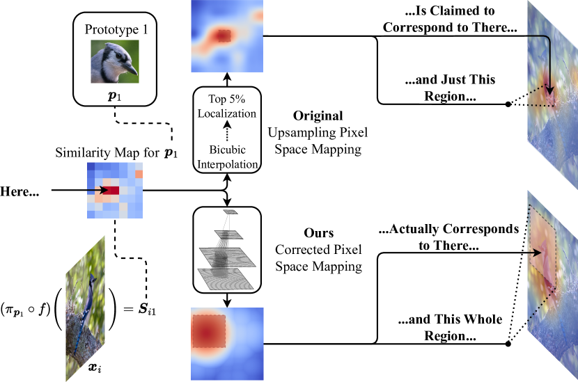
Figure 1: The two primary issues identified with prototype visualization: here (this embedded patch) does not correspond to there (this image patch), and this (prototype) does not correspond to just that (test image patch). In the extreme case, this can actually correspond to the entire image (i.e., when the receptive field is 100%).

ProtoPartNNs approach explainability from an intrinsically interpretable lens and offer many benefits over post hoc explanation. Whereas post hoc explainers estimate an explanation, ProtoPartNN explanations are part of the actual prediction process – explanations along the lines of “this looks like that” follow naturally from the symbolic form of the model itself. This implicit explanation is characteristic of models widely considered to be human-comprehensible [63]. Moreover, ProtoPartNNs enable concept-level debugging, human-in-the-loop learning, and implicit localization [58, 55, 13]. Being independent of the explained model, post hoc explainers have been found to be unfaithful, inconsistent, and unreliable [47, 79, 38, 10] (see Section 2 for expanded discussion).

When misunderstood or used inappropriately, explainable AI (XAI) methods can have unintended consequences [39, 47]. This harm arises from unverified hypotheses, whether it is that explanations represent phenomena faithful to the predictor or meaningful properties of the predictor. So, why do we see such hypotheses proliferating throughout both academia and industry [48, 39]? The problem is very human – there is often an over-reliance on intuition that may lead to illusory progress or deceptive conclusions. Whether it is dependence on alluring visualization or behavioral extrapolation from cherry-picked examples, XAI methods often are left insufficiently scrutinized and subject to “researcher degrees of freedom” [72, 48].

Recent evidence indicates that ProtoPartNNs may suffer from these same issues: ProtoPNet and its variants exhibit irrelevant prototypes, a human-machine semantic similarity gap, and exorbitant explanation size [78, 43, 34]. Unfortunately, in our study, we confirm that this is the case – there are several facets of existing ProtoPartNN explanations that do not result from the implicit form of the model: object part localization, pixel space grounding, and heat map visualizations. Instead, these are founded on unverified assumptions and an over-reliance on intuition, often justified a posteriori by attractive visuals. We demonstrate that, colloquially, this does not actually look like that, and here may not actually correspond to there – see Figure 1 for illustration. These issues with ProtoPartNNs are not limited to just ProtoPNet, but to all of its derivatives.

This work aims to elevate the interpretability of ProtoPartNNs by rectifying these facets. In doing so, all aspects of ProtoPartNN explanations are embedded in the symbolic form of the model. Our contributions are as follows:

• We identify that existing ProtoPartNNs based on ProtoPNet do not localize faithfully nor actually localize to object parts, but rather the full image in most cases.

• We propose a novel pixel space mapping based on the receptive fields of an architecture (we guarantee that here corresponds to there).

• We propose architectural constraints that we efficiently discover through a transfer task to enable true object part localization (this looks like that).

• We devise a novel functional algorithm for the receptive field calculation of any architecture.

• On several image classification tasks, our approach, PixPNet, achieves competitive accuracy with other ProtoPartNNs while maintaining a higher degree of interpretability, as substantiated by functionally grounded XAI metrics, and being the only ProtoPartNN that truly localizes to object parts.

2 Background

In this section, we give a brief background of explainable AI methods, the ProtoPNet formulation, and an overview of ProtoPNet extensions.

Explainable AI Methods

Explainable AI (XAI) solutions can be classified as post hoc, intrinsically interpretable, or a hybrid of the two [71]. Whereas intrinsically interpretable methods are both the explanator and predictor, post hoc methods act as an explanator for an independent predictor. Unfortunately, post hoc explainers are known to be inconsistent, unfaithful, and possibly even intractable [47, 7, 15, 26, 10]. Furthermore, they are deceivable [79, 17, 18, 3] and have been shown to not affect, or even reduce, end-user task performance [38, 37]. While this is the case, post hoc explanations have been shown to possibly increase user trust in AI systems [12], improve end-user performance for some explanation types and tasks [37], and explain black boxes in trustless auditing schemes [11]. However, for high-stakes domains, post hoc explanation is frequently argued to be especially inappropriate [66].

For these numerous reasons, our work concerns intrinsically interpretable machine learning solutions (see [71] for a methodological overview). In particular, we are interested in prototypical part neural networks (ProtoPartNNs) [13].

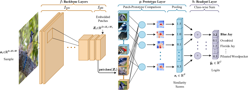
(a) PixPNet (Pixel-grounded Prototypical part Network) architecture.

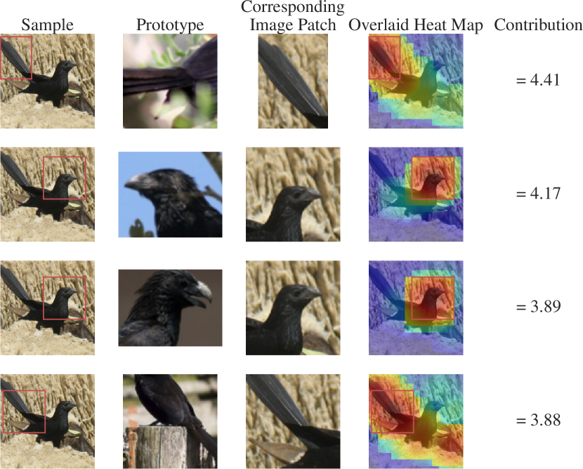
(b) An example of an explanation.

Figure 2: (a) Our proposed architecture, PixPNet. (b) An example of an explanation with PixPNet for a Groove-billed Ani. The following are important deviations from ProtoPNet: the backbone ${f}$ receptive field is constrained, the readout layer ${h}$ is simplified, both prototypes and embedded patches truly localize to object parts, and the pixel space mapping is corrected (see Figure 3).

ProtoPNet Architecture

Here, we go over the ProtoPNet architecture [13], a type of ProtoPartNN. As much of the formalism overlaps with our approach, Figure 2 can be referred to for visualization of the architecture. Let ${{\bm{\mathsfit{D}}}}{=}\{({{\bm{x}}}_{1},{y}_{1}),({{\bm{x}}}_{2},{y}_{2}),\dots,({{\bm{x}}}_{N},{y}_{N})\}$ be the data set where each sample ${{\bm{x}}}_{i}{\in}{\mathbb{R}}^{3\times H\times W}$ is an image with a height of $H$ and a width of $W$, and each label ${y}_{i}{\in}\{1,\dots,C\}$ represents one of $C$ classes.

A ProtoPNet comprises a neural network backbone responsible for embedding an image. The first component of the backbone is the core ${f_{\text{core}}}$, which could be a ResNet [30], VGG [73], or DenseNet [35] as in [13]. Proceeding, there are the add-on layers ${f_{\text{add}}}$ that are responsible for changing the number of channels in the output of ${f_{\text{core}}}$. In ProtoPNet, ${f_{\text{add}}}$ comprises two $1\times 1$ convolutional layers with ReLU and sigmoid activation functions for the first and second layers, respectively. The full feature embedding function is denoted by ${f}={f_{\text{add}}}\circ{f_{\text{core}}}$. This function gives us our embedded patches ${f}({{\bm{x}}}_{i})={{\bm{Z}}}_{i}\in{\mathbb{R}}^{D\times H_{z}\times W_{z}}$ which have $D$ channels, a height of $H_{z}$, and a width of $W_{z}$.

In ProtoPNet, we are interested in finding the most similar embedded patch ${{\bm{z}}}$ for each prototype. Each prototype can be understood as the embedding of some prototypical part of an object, such as the head of a blue jay as in Figure 2. Each embedded patch can be thought of in the same way – ultimately, a well-trained network will find that the most similar embedded patch and prototype will both be, e.g., the head of a blue jay (this prototype looks like that embedded patch). This is accomplished using the prototype layer, ${g}$. We use the notation ${g}_{{{\bm{p}}}_{j}}$ to denote the unit that computes the most similar patch ${{\bm{z}}}{\in}{\small\texttt{patches}}({{\bm{Z}}}_{i})$ to prototype ${{\bm{p}}}_{j}$. The function ${\small\texttt{patches}}({{\bm{Z}}}_{i})$ yields a set of $D{\times}H_{p}{\times}W_{p}$ embedded patches in a sliding window manner ($H_{p}{=}W_{p}{=}1$ in ProtoPNet). First, the pairwise distances between ${\small\texttt{patches}}({{\bm{Z}}}_{i})$ and prototypes ${{\bm{P}}}{=}\{{{\bm{p}}}_{j}\}^{P}_{j=1}$ are computed using a distance function ${\varphi}$ where ${{\bm{p}}}_{j}{\in}{\mathbb{R}}^{D{\times}H_{p}{\times}W_{p}}$, $H_{p}$ is the prototype kernel height, $W_{p}$ is the prototype kernel width, and $P$ is the total number of prototypes. Each prototype is class-specific and we denote the set of prototypes belonging to class ${y}_{i}$ as ${{\bm{P}}}_{{y}_{i}}{\subseteq}{{\bm{P}}}$. Subsequently, a min-pooling operation is performed to obtain the closest embedded patch for each prototype – each prototype (this) is “assigned” a single embedded patch (that). Finally, the distances are converted into similarity scores using a similarity function ${v}$. Putting this process altogether for unit ${g}_{{{\bm{p}}}_{j}}$, we have

$${g}_{{{\bm{p}}}_{j}}({{\bm{Z}}}_{i})={v}\Big{(}\min_{{{\bm{z}}}\in{\small\texttt{patches}}({{\bm{Z}}}_{i})}{\varphi}({{\bm{z}}},{{\bm{p}}}_{j})\Big{)}.$$ (1)

We denote the vector of all similarity scores for a sample as ${{\bm{s}}}_{i}={g}({{\bm{Z}}}_{i})\in{\mathbb{R}}^{P}$.

The architecture ends with a readout layer ${h}$ that produces the logits as ${\hat{{\bm{y}}}}_{i}={h}({{\bm{s}}}_{i})$. In ProtoPNet, ${h}$ is a fully-connected layer with positive weights to same-class prototype units and negative weights to non-class prototype units. Each logit can be interpreted as the sum of similarity scores weighed by their importance to the class of the logit. Note that this readout layer is not reflected in Figure 2. The full ProtoPNet output for a sample is given by $({h}\circ{g}\circ{f})({{\bm{x}}}_{i})$.

ProtoPartNN Desiderata and ProtoPNet Variants

Many extensions of ProtoPNet have been proposed, some of which make altercations that fundamentally affect the interpretability of the architecture. To differentiate these extensions, we propose a set of desiderata for ProtoPartNNs:

1. Prototypes must correspond directly to image patches. This can be accomplished via prototype replacement, which grounds prototypes in human-interpretable pixel space (see Section 4 for details).

2. Prototypes must localize to object parts.

3. Case-based reasoning must be describable by linear or simple tree models.

Architectures that satisfy all three desiderata are considered to be 3-way ProtoPartNNs – satisfying fewer diminishes the interpretability of the algorithm.

The idea of sharing prototypes between classes has been explored in ProtoPShare [68] (prototype merge-pruning) and ProtoPool [67] (differential prototype assignment). In ProtoTree [59], the classification head is replaced by a differentiable tree, also with shared prototypes. An alternative embedding space is explored in TesNet [87] based on Grassmann manifolds. A ProtoPartNN-specific knowledge distillation approach is proposed in Proto2Proto [40] by enforcing that student prototypes and embeddings should be close to those of the teacher. Deformable ProtoPNet [20] extends the ProtoPNet architecture with deformable prototypes. ST-ProtoPNet [86] learns support prototypes that lie near the classification boundary and trivial prototypes that are far from the classification boundary.

In an attempt to improve ProtoPNet visualizations, an extension of layer-wise relevance propagation [2], Prototypical Relevance Propagation (PRP), is proposed to create more model-aware explanations [28]. PRP is quantitatively more effective in debugging erroneous prototypes and assigning pixel relevance than the original approach.

ProtoPartNN-Like Methods

The following papers are inspired by ProtoPNet but cannot be considered to be the same class of model. This is due to not fulfilling the proposed ProtoPartNN desiderata #1 (prototypes must correspond directly to image patches) and/or #3 (case-based reasoning must be describable by linear or simple tree models).

ViT-NeT [42] combines a vision transformer (ViT) with a neural tree decoder that learns prototypes. In another transformer-based approach, ProtoPFormer [88] exploits the inherent architectural features (local and global branches) of ViTs. Semi-ProtoPNet [80] fixes the readout weights as NP-ProtoPNet [77] does and is used for power distribution network analysis. In SDFA-SA-ProtoPNet [36], a shallow-deep feature alignment (SDFA) module aligns the similarity structures between deep and shallow layers. In addition, a score aggregation (SA) module aggregates similarity scores to avoid learning inter-class information. Unfortunately, each of these networks omits prototype replacement with the typical justification being that doing so improves task accuracy. In addition, ViT-NeT has additional layers after ${g}$ that break the mapping back to pixel space and complicate its case-based reasoning.

3 The Problem with Existing ProtoPartNNs

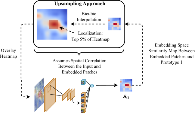
(a) The original upsampling-based pixel space mapping.

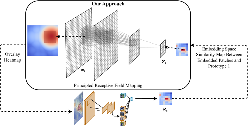
(b) Our proposed receptive field-based pixel space mapping.

Figure 3: Visualization of the original and proposed pixel space mapping approaches.

Despite the many extensions of ProtoPNet, there are still fundamental issues with object part localization, pixel space grounding, and heat map visualizations, which preclude any existing ProtoPartNN from satisfying all three desiderata – all ProtoPartNNs violate desideratum #2: prototypes must localize to object parts. The underlying issues with existing ProtoPartNNs arise from 1) their pixel space mapping being reliant on spatial correlation between embedded patches and the input space, which is dubious; 2) their pixel space mapping being receptive field-invariant, arbitrarily localizing to some area in the input. Rather, intrinsically interpretable models should produce explanations implicit in the symbolic form of the model itself [63, 71].

As a refresher, the original visualization process involves three steps. First, a single similarity map ${{\bm{S}}}_{ij}{=}{\pi}_{{{\bm{p}}}_{j}}({{\bm{Z}}}_{i})\in{\mathbb{R}}^{H_{z}/H_{p}\times W_{z}/W_{p}}$ is selected for visualization where ${\pi}_{{{\bm{p}}}_{j}}$ gives the similarity map for prototype ${{\bm{p}}}_{j}$. Each element of ${{\bm{S}}}_{ij}$ is given by ${v}\left({\varphi}({{\bm{z}}},{{\bm{p}}}_{j})\right)$ where ${{\bm{z}}}{\in}{\small\texttt{patches}}({{\bm{Z}}}_{i})$. Subsequently, this map is upsampled from $H_{z}/H_{p}{\times}W_{z}/W_{p}$ to $H{\times}W$ using bicubic interpolation, producing a heat map ${\bm{M}}_{ij}{\in}{\mathbb{R}}^{H{\times}W}$. To localize within the image, the smallest bounding box is drawn around the largest 5% of heat map elements – this box is of variable size. While no justification is provided for this approach in the original paper [13], we believe that the intuition is that the embedded patches ${{\bm{Z}}}_{i}$ maintain spatial correlation with the input. Finally, ${\bm{M}}_{ij}$ and the bounding box can be superimposed on the input image for visualization. From here on out, we will refer to this as the original pixel space mapping, which is visualized in Figure 3(a). It should also be noted that while this pixel space mapping is crucial in establishing interpretability, it is left undiscussed in the vast majority of ProtoPNet extensions. Immediately, we can see several issues with this approach.

Here Does Not Correspond to There

The original pixel space mapping is based on naive upsampling, which is invariant to architectural details. The approach will always assume that all similarity scores can be mapped to pixel space with a single linear transformation – an embedded patch at position $\langle t_{x},t_{y}\rangle$ is effectively localized to position $\langle t_{x}{\cdot}W{\cdot}W_{p}/W_{z},t_{y}{\cdot}H{\cdot}H_{p}/H_{z}\rangle$ in pixel space. This assumption of spatial correlation from high to low layers is easy to invalidate. For instance, even a simple latent transpose eradicates this correlation. The similarity scores of embedded patches do not determine where the architecture “looked” in the image. Rather, the architecture determines where the similarity scores correspond to in the image. Figure 1 demonstrates this discrepancy. Very recently, evidence in [33, 69] strongly corroborates our arguments about poor localization. We correct this pixel space mapping according to the receptive fields of the underlying neural architecture. The original approach also only provides a way to localize a prototype rather than any embedded patch – our method enables us to do so. Our approach is described in detail in Section 4 and we validate its correctness over the original approach in Section 5.

This Does not Correspond to Just That

ProtoPNet and its derivatives all elect to localize to a small region of the input by drawing a bounding box around the largest 5% of values of heat map ${\bm{M}}_{ij}$ as shown in Figure 3(a). While this produces alluring visualizations, most of the architectures evaluated in all prior approaches have a mean receptive field of 100% at the embedding layer. A mean receptive field of 100% means that every element of the embedding layer output is a complex function of every pixel in the input space. Is it fair to say that only $\sim$5% of the input contributed to some part of a decision? Attribution within the input space spanned by a receptive field is unverifiable from both the feature-selectivity and feature-additivity points of view [9, 48]. This issue is visualized in Figure 1 for an architecture with a mean receptive field under 100%. Moreover, while selecting the top 5% of ${\bm{M}}_{ij}$ may localize in accordance with its (faulty) intuition, it can actually localize to wildly inaccurate parts of the image (e.g., if multiple top values in ${{\bm{S}}}_{ij}$ are all close), breaking the intuition of the (unfaithful) pixel space mapping. We go on to discuss our solution to this problem in Section 4.

The Allure of Visualization

The original pixel space mapping appears to satisfy human intuitions. However, it is not based on well-justified aspects of explainability. Beyond the assumption of spatial correlation and naive localization, bicubic interpolation artificially increases the resolution of maps (see Figure 3(a)), which leads non-experts to believe that per-pixel attributions are estimated. In our proposed approach, these explanation aspects follow naturally from the symbolic interpretation of the model itself.

4 Fixing ProtoPartNNs

As discussed in Section 3, the underlying issues with ProtoPartNNs arise from 1) the original pixel space mapping being reliant on spatial correlation between embedded patches and the input space, which is dubious; 2) the original pixel space mapping being receptive field-invariant, arbitrarily localizing to some area in the input. Our proposed architecture, PixPNet (Pixel-grounded Prototypical part Network), is largely based on ProtoPNet but mitigates these issues through symbolic interpretation of its architecture – see Figure 2 for an overview. In this section, we first describe a new algorithm for the calculation of receptive fields, describe our proposed fixes for prototype visualization and localization, and proceed with additional ProtoPartNN corrections and improvements. With the proposed improvements, PixPNet is the only ProtoPartNN that truly localizes to object parts, satisfying all three desiderata.

Receptive Field Calculation Algorithm

Before delving into our proposed remedies, we describe our approach to computing receptive fields precisely for any architecture. Our proposed algorithm, FunctionalRF, takes a neural network as input and outputs the exact receptive field of every neuron in the neural network. Recall that a neuron is a function of a subset of pixels defined by its receptive field. FunctionalRF represents receptive fields as hypercubes (multidimensional tensor slices). For instance, the slices for a 2D convolution with a $5{\times}5$ kernel, stride of 1, and $c_{\text{in}}$ channels at output position $3,3$ would be $\{\{\llbracket 1,c_{\text{in}}\rrbracket,\llbracket 1,5\rrbracket,\llbracket 1,5\rrbracket\}\}$ where $\llbracket a,b\rrbracket$ denotes the slice between $a$ and $b$. We can compute the mean receptive field of a layer as the average number of pixels within the receptive field of each hypercube element of a layer output. The algorithm does not rely on approximate methods nor architectural alignment assumptions like other approaches [52, 1]. The full algorithmic details are provided in Appendix C.

Corrected Pixel Space Mapping Algorithm

From Embedding Space to Pixel Space   For each prototype ${{\bm{p}}}_{j}$, we have some ${{\bm{z}}}\in{{\bm{Z}}}_{i}$ that is most similar. We are interested in knowing where ${{\bm{z}}}$ localizes to in an image ${{\bm{x}}}_{i}$. With FunctionalRF applied to the backbone, we have the precise pixel space region that ${{\bm{z}}}$ is a function of – this exactly corresponds to that. This can also be done for any ${{\bm{p}}}_{j}$ after prototype replacement. Additionally, this process can actually be used to visualize any ${{\bm{z}}}\in{{\bm{Z}}}_{i}$, unlike the procedure specified in the original pixel space mapping [13]. See Figure 3(b) for intuition as to how this process works.

Producing a Pixel Space Heat Map   In order to compute a pixel space heat map, we propose an algorithm based on FunctionalRF rather than naively upsampling an embedding space similarity map ${{\bm{S}}}_{ij}$. Our approach uses the same idea as going from embedding space to pixel space. Each pixel space heat map ${\bm{M}}_{ij}\in{\mathbb{R}}^{H\times W}$ is initialized to all zeros ($\mathbf{0}^{H\times W}$), and corresponds to a sample ${{\bm{x}}}_{i}$ and a prototype ${{\bm{p}}}_{j}$. Let ${\bm{M}}_{ij}^{S}$ be the region of ${\bm{M}}_{ij}$ defined by the receptive field of similarity score ${S}\in{{\bm{S}}}_{ij}$. For each ${S}$, the pixel space heat map is updated as ${\bm{M}}_{ij}^{S}\leftarrow\max({\bm{M}}_{ij}^{S},{S})$ where $\max(\cdot)$ is an element-wise maximum that appropriately handles the case of overlapping receptive fields. We take maxima instead of averaging values due to Eq. (1). Again, see Figure 3(b) for a visualization of this procedure. Further algorithmic details are provided in Appendix D.

Improved Localization & the “Goldilocks” Zone

To reiterate, the region localized by a ProtoPartNN is controlled by the receptive field of the embedding layers of ${f}$. A fundamental goal of ProtoPartNNs is to identify and learn prototypical object parts. We propose to achieve this by constraining the receptive field of ${f}$ to a range that yields object parts that are both meaningful and interpretable to humans.

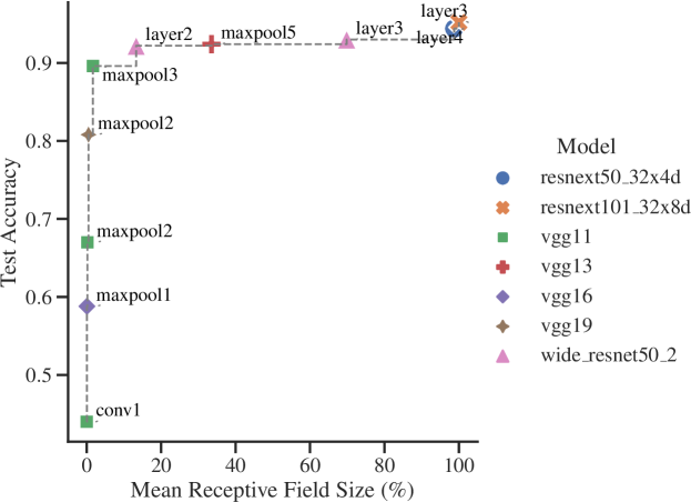
Figure 4: The Pareto front of architectures trained on ImageNette [25] and evaluated at various intermediate layers. This front details the accuracy-localization size trade-offs and informs backbone selection of PixPNet as in Section 5.

It is well known that the receptive field of a neural network correlates with performance [52, 1] to an extent – too small or large a receptive field can harm performance due to bias-variance trade-offs [45]. We hypothesize that there is a “Goldilocks” zone where the desired receptive field localizes to intelligible object parts without diminishing task performance. To corroborate this, we evaluate various backbone architectures at intermediate layers on ImageNette [25], a subset of ImageNet [16]. The evaluation aims to produce architectures suitable for the backbone of PixPNet according to the criteria outlined prior. We propose this approach as performance on subsets of ImageNet has been shown to be reflective of performance on the full dataset [19], and ImageNet performance strongly correlates with performance on other vision datasets [44]. We detail the full experiment setup in Appendix F. The Pareto front of mean receptive field and accuracy for the evaluated architectures is shown in Figure 4. This front informs our backbone selection as detailed in Section 5.

Simplified Classification Head

While the original fully-connected classification head ${h}$ is human-interpretable, it has several weaknesses – its explanation size limits its comprehension [78, 43] and it requires an additional training stage, adding up to 100 additional epochs in ProtoPNet. We quantify explanation size in terms of positive reasoning and negative reasoning about the prediction of a class. For positive reasoning, the number of elements in an explanation with the original fully-connected layer is $2P/C$: one similarity score per class-specific prototype and a positive weight coefficient. However, considering both positive and negative reasoning involves $2P$ total explanation elements.

To address these limitations, we propose to replace the linear layer with a class-wise summation. This operation simply produces the logit of each class as the sum of class-specific similarity scores as $\hat{{y}}_{ic}=\sum_{j:{{\bm{p}}}_{j}\in{{\bm{P}}}_{c}}{s}_{ij}$ where $\hat{{y}}_{ic}$ is the logit for class $c$ and ${s}_{ij}$ is the similarity score for prototype ${{\bm{p}}}_{j}$. The layer is visualized in Figure 2. Our new parameter-free readout layer removes the additional training stage and comprises only $P/C$ explanation elements for both positive and negative reasoning. Substituting our layer in the original ProtoPNet configuration for the CUB-200-2011 dataset [13, 85] reduces the number of explanation elements for a class prediction from 4,000 down to just 10.

Other Improvements

We also make a few smaller contributions. In prototype replacement, we remove duplicate prototypes (by image or sample) to encourage diversity. If duplicates are found, the next most-similar embedded patch is used in replacement instead. We also reformulate the similarity function ${v}$ to have lower numerical error (see Appendix G for details) as ${v}(d){=}\log(\frac{1}{d{+}\varepsilon}{+}1)$ where $\varepsilon$ mitigates division by zero and the distance $d{=}{\varphi}({{\bm{z}}},{{\bm{p}}}_{j})$. While ProtoPNet uses ${\varphi}({{\bm{z}}},{{\bm{p}}}_{j}){=}\lVert{{\bm{z}}}-{{\bm{p}}}_{j}\rVert_{2}^{2}$, we elect to use ${\varphi}({{\bm{z}}},{{\bm{p}}}_{j}){=}1-\frac{{{\bm{z}}}\cdot{{\bm{p}}}}{\lVert{{\bm{z}}}\rVert_{2}\lVert{{\bm{p}}}\rVert_{2}}$ (cosine distance), which has a desirable normalizing factor. This distance is also used in [87, 5, 20, 41]. In implementation, the distances are computed using generalized convolution [57, 29, 13].

BBox	D1	D2	D3	Model	$f$	Expl. Size $+$	Expl. Size $\pm$	$P$	MRF	Acc.	$\pm$	$S_{\text{con}}$	$S_{\text{sta}}$	Code Avail.	Val. Set
✗	✓	✓	✓	PixPNet (Ours)	ResNeXt@layer3	10	10	2000	100	81.76	0.2	56.4	64.7	✓	✓
				PixPNet (Ours)	VGG19@maxpool5	10	10	2000	70.4	80.10	0.1	47.6	64.2	✓	✓
				PixPNet (Ours)	VGG16@maxpool5	10	10	2000	52.5	79.75	0.2	69.5	51.6	✓	✓
				PixPNet (Ours)	VGG13@maxpool4	10	10	2000	9.69	75.32	0.2	66.9	45.0	✓	✓
	✓	✗	✓	ST-ProtoPNet [86]	DenseNet161	20	4000	2000	100	80.60	–	–	–	✗	?
✓	✓	✗	✓	ST-ProtoPNet [86]	DenseNet161	20	4000	2000	100	86.10	0.2	–	–	✗	?
				TesNet [87]	DenseNet121	20	4000	2000	100	84.80	0.2	63.1	66.1	✓	✗
				ProtoPool [67]	ResNet152	20	404	202	100	81.50	0.1	35.7	58.4	✓	✗
				ProtoPNet [13]	DenseNet121	20	4000	2000	100	80.20	0.2	24.9	58.9	✓	✗
				Proto2Proto [40]	ResNet34	20	4000	2000	100	79.89	–	–	–	✓	✗
				ProtoPShare [68]	DenseNet161	1200	1200	600	100	76.45	–	–	–	✓	✗
				ProtoTree [59, 36]	DenseNet121	18	404	202	100	73.20	–	21.5	24.4	✓	✗
✗	✗	✗	✓	ProtoPFormer [88]	DeiT-S	40	8000	4000	100	84.85	–	–	–	✓	✗
	✗	✗	✗	ViT-NeT [42, 88]	CaiT-XXS-24	8	30	15	100	84.51	–	–	–	✓	✗
✓	✗	✗	✗	ViT-NeT [42]	SwinT-B	10	62	31	100	91.60	–	–	–	✓	✗
?	✗	✗	✓	SDFA-SA [36]	DenseNet161	20	20	2000	100	86.80	–	73.2	73.5	✗	?

Table 1: ProtoPartNN results on CUB-200-2011 with ImageNet used for pre-training. Columns D1, D2, and D3 correspond to the three desiderata established in Section 2. Our approach, PixPNet, is the only method that is a 3-way ProtoPartNN, satisfying all three desiderata. “BBox” indicates whether a method crops each image using a bounding box annotation. The best results of ProtoPartNNs with and without such annotations are bold and underlined, respectively. The table is split based on whether the method meets at least two desiderata. The $S_{\text{con}}$ and $S_{\text{sta}}$ scores for other methods are taken from [36] and the top reported accuracy score is taken for each method.

Training

Our multi-stage training procedure is similar to that of ProtoPNet. The first stage optimizes the full network, except for the readout layer, by minimizing Eq. (2) via stochastic gradient descent

$$\begin{split}\frac{1}{N}\sum_{i=1}^{N}{\mathcal{L}_{\text{xent}}}({\hat{{\bm{y}}}}_{i},{y}_{i}){+}{\lambda_{\text{cls}}}{\mathcal{L}_{\text{cls}}}({{\bm{P}}},{{\bm{Z}}}_{i}){+}{\lambda_{\text{sep}}}{\mathcal{L}_{\text{sep}}}({{\bm{P}}},{{\bm{Z}}}_{i})\end{split}$$ (2)

where ${\mathcal{L}_{\text{xent}}}$ is the categorical cross-entropy loss function, ${\lambda_{\text{cls}}}$ and ${\lambda_{\text{sep}}}$ are auxiliary loss weights, and the auxiliary loss functions, ${\mathcal{L}_{\text{cls}}}$ and ${\mathcal{L}_{\text{sep}}}$, are defined as

$${\mathcal{L}_{\text{cls}}}({{\bm{P}}},{{\bm{Z}}}_{i}) =\frac{1}{N}\sum_{i=1}^{N}\min_{\begin{subarray}{c}{{\bm{p}}}_{j}\in{{\bm{P}}}_{{y}_{i}}\\ {{\bm{z}}}\in{\small\texttt{patches}}({{\bm{Z}}}_{i})\end{subarray}}{\varphi}({{\bm{z}}},{{\bm{p}}}_{j})$$ (3)

$${\mathcal{L}_{\text{sep}}}({{\bm{P}}},{{\bm{Z}}}_{i}) =-\frac{1}{N}\sum_{i=1}^{N}\min_{\begin{subarray}{c}{{\bm{p}}}_{j}\notin{{\bm{P}}}_{{y}_{i}}\\ {{\bm{z}}}\in{\small\texttt{patches}}({{\bm{Z}}}_{i})\end{subarray}}{\varphi}({{\bm{z}}},{{\bm{p}}}_{j}).$$ (4)

The goal of ${\mathcal{L}_{\text{cls}}}$ is to ensure that at least one embedded patch of every training image is similar to at least one prototype belonging to the class of the image. In contrast, the goal of ${\mathcal{L}_{\text{sep}}}$ is to ensure that the embedded patches of every training image are dissimilar from prototypes not belonging to the class of the image.

Subsequently, the prototypes are replaced, which is arguably the most important stage of training as it grounds prototypes in human-comprehensible pixel space. The process involves replacing each prototype ${{\bm{p}}}_{j}$ with an embedded patch ${{\bm{z}}}$ of a training sample of the same class – the most similar embedded patch replaces the prototype. In the literature, prototype replacement is also referred to as prototype “pushing” or “projection.” We stick with “replacement” for the sake of clarity. Formally, this update can be written as ${{\bm{p}}}_{j}\,{\leftarrow}\,\operatorname*{arg\,min}_{{{\bm{z}}}\in{\small\texttt{patches}}({{\bm{Z}}}_{i})}{\varphi}({{\bm{z}}},{{\bm{p}}}_{j}),\text{ s.t. }{{\bm{p}}}_{j}\,{\in}\,{{\bm{P}}}_{{y}_{i}}$. Without this update, the human interpretation of prototypes is unclear as prototypes are not grounded in pixel space.

In ProtoPNet and its variants, a third stage optimizes the linear readout layer. However, we do not employ this stage as our readout layer is parameter-free. The multi-stage optimization process can be repeated until convergence.

5 Experiments & Discussion

To validate our proposed approach, PixPNet, we evaluate both its accuracy and interpretability on CUB-200-2011 [85]. We also show evaluation results on Stanford Cars [46] in Appendix B. We draw comparisons against other ProtoPartNNs with a variety of measures. We elect to not crop images in CUB-200-2011 by their bounding box annotations to demonstrate the localization capability of PixPNet. Hyperparameters, software, hardware, and other reproducibility details are specified in Appendix E.

Lastly, upon inspection of the original code base, we discovered that the test set accuracy is used to influence training of ProtoPNet. In fact, neither ProtoPNet nor its extensions for image classification that are mentioned in Section 2 employ a validation set in provided implementations. See Appendix H for further details.

In our implementation, we employ a proper validation set and tune hyperparameters only according to accuracy on this split.

Accuracy

The experimental results in Table 4 show that PixPNet obtains competitive accuracy with other approaches regardless of whether images are cropped by bird bounding box annotations – while we trade off network depth for interpretability, we outperform ProtoPNet and several of its derivatives. This is quite favorable as PixPNet is the only method that truly localizes to object parts.

Interpretability

We evaluate the interpretability of our approach with several functionally grounded metrics [21]. See Figure 2(b) for an example of a PixPNet explanation.

Relevance Ordering Test (ROT)   The ROT is a quantitative measure of how well a pixel space mapping attributes individual pixels according to prototype similarity scores [28]. First, a pixel space heat map ${\bm{M}}_{ij}$ is produced for a single sample ${{\bm{x}}}_{i}$ and prototype ${{\bm{p}}}_{j}$. Starting from a completely random image, pixels are added back to the random image one at a time in descending order according to ${\bm{M}}_{ij}$. As each pixel is added back, the similarity score for ${{\bm{p}}}_{j}$ is evaluated. This procedure is averaged over each class-specific prototype over 50 random samples. The faster that the original similarity score is recovered, the better the pixel space mapping is. Assuming a faithful pixel space mapping, a network with a mean receptive field of, e.g., 25%, will recover the original similarity score after 25% of the pixels are added back in the worst-case scenario.

We also introduce two aggregate measures of the ROT. First is the area under the similarity curve (AUSC) which is normalized by the difference between the original similarity score and the baseline value (similarity score for a completely random image). Second is the percentage of pixels added back to recover the original similarity score: pixel percentage to recovery (%2R).

Backbone	MRF	Acc. ↑	PSM	$S_{\text{con}}$ ↑	$S_{\text{sta}}$ ↑	AUSC ↑	%2R ↓
VGG11 @maxpool4	8.31	72.9	Ours	65.3	48.3	0.99	11.2
			Orig.	45.8	44.0	0.90	30.5
VGG13 @maxpool4	9.69	75.3	Ours	66.9	45.0	0.97	13.0
			Orig.	48.1	41.8	0.88	84.1
VGG16 @maxpool4	15.7	76.4	Ours	62.0	46.4	1.02	6.98
			Orig.	46.8	42.2	0.89	35.5
VGG19 @maxpool4	22.8	77.1	Ours	60.1	42.5	0.94	21.4
			Orig.	48.4	41.3	0.80	99.9
VGG13 @maxpool5	33.5	78.1	Ours	67.0	42.5	0.90	29.5
			Orig.	43.7	39.9	0.81	99.2
VGG16 @maxpool5	52.5	79.8	Ours	69.5	51.6	0.90	32.0
			Orig.	44.1	42.4	0.82	55.5
WRN50 @layer3	69.9	80.1	Ours	56.4	64.7	0.93	13.0
			Orig.	56.4	47.6	0.85	39.6
VGG19 @maxpool5	70.4	80.1	Ours	47.6	64.2	0.92	43.4
			Orig.	45.8	46.0	0.85	92.9
ResNet18 @layer2	15.4	57.2	Ours	59.2	46.6	0.98	4.10
			Orig.	25.2	45.6	0.88	96.8
			PRP	–	–	0.95	25.4
ResNet50 @layer3	69.8	76.6	Ours	47.9	62.0	0.58	72.8
			Orig.	53.5	42.7	0.42	97.8
			PRP	–	–	0.34	100.0

Table 2: Evaluation of pixel space mapping (PSM) methods with functionally-grounded interpretability metrics. Methods are compared on PixPNet with “Goldilocks” zone and ResNet backbones on CUB-200-2011 (no BBox cropping). Our PSM outperforms both the original and PRP PSMs across all backbones.

We compare our pixel space mapping to the original upsampling approach and PRP [28]. However, the PRP implementation only supports ResNet architectures, so it is not included in all experiments. The results in Table 2 demonstrate that our pixel space mapping best identifies the most important pixels in an image. Naturally, the mean receptive field correlates with both ROT scores.

Explanation Size   Recall from Section 4 that the explanation size is the number of elements in an explanation, i.e., similarity scores and weight coefficients. This number differs when considering positive or negative reasoning. Due to the original classification head being fully-connected, most ProtoPartNNs have large explanation sizes when considering both positive and negative reasoning, as shown in Table 4. In contrast, our explanation size comprises just 10 elements when reasoning about a decision. Our proposed classification head helps to prevent overwhelming users with information, which has been shown to be the case with other ProtoPartNNs [43].

Consistency   The consistency metric [36] quantifies how consistently each prototype localizes to the same human-annotated ground truth part. It evaluates both semantic similarity quality and the pixel space mapping to a degree. For a sample ${{\bm{x}}}_{i}$ with label ${y}_{i}$, the pixel space mapping is computed for each prototype ${{\bm{p}}}_{j}\in{{\bm{P}}}_{{y}_{i}}$. Let $o_{{{\bm{p}}}_{j}}({{\bm{x}}}_{i})\in{\mathbb{R}}^{K}$ be a binary vector indicating which of $K$ object parts are contained within the region localized by the pixel space mapping. Let $u({{\bm{x}}}_{i})\in{\mathbb{R}}^{K}$ be a binary vector indicating which of the $K$ object parts are actually visible in ${{\bm{x}}}_{i}$. A single object part is associated with ${{\bm{p}}}_{j}$ by taking the maximum frequency of an object part present in the pixel space mapping region across all applicable images. A prototype is said to be consistent if this frequency is at least $\mu$, i.e.,

$$S_{\text{con}}=\frac{1}{P}\sum_{j=1}^{P}\mathbbm{1}\Bigg{[}\max\Bigg{(}\sum_{{{\bm{x}}}_{i}\in{{\bm{\mathsfit{X}}}}_{c_{j}}}\left(o_{{{\bm{p}}}_{j}}({{\bm{x}}}_{i})\oslash u({{\bm{x}}}_{i})\right)\Bigg{)}\geq\mu\Bigg{]}$$

where ${{\bm{\mathsfit{X}}}}_{c_{j}}$ are samples of the same class allocated to ${{\bm{p}}}_{j}$, $\oslash$ denotes element-wise division, and $\mathbbm{1}$ is the indicator function. To compare with results reported in [36], we change the receptive field size in our pixel space mapping to equal this, as well as set $\mu=0.8$. A notable weakness of the evaluation approach is that it uses a fixed $72\times 72$ pixel region independent of the architecture. While the approach is not perfect, it allows for reproducible and comparative interpretability evaluation between ProtoPartNN variants.

Results are shown in Tables 4 and 2 for CUB-200-2011, which provides human-annotated object part annotations. We outperform ProtoPNet and many of its variants, as well as the original pixel space mapping (Table 2).

Stability   The stability metric [36] measures how robust object part association is when noise is added to an image. Simply, some noise $\epsilon\sim\mathcal{N}(0,\sigma^{2})$ is added to each sample ${{\bm{x}}}_{i}$ and the object part associations are compared as

$$S_{\text{sta}}=\frac{1}{P}\sum_{j=1}^{P}\frac{\sum_{{{\bm{x}}}_{i}\in{{\bm{\mathsfit{X}}}}_{c_{j}}}\mathbbm{1}\left[o_{{{\bm{p}}}_{j}}({{\bm{x}}}_{i})=o_{{{\bm{p}}}_{j}}({{\bm{x}}}_{i}+\epsilon)\right]}{|{{\bm{\mathsfit{X}}}}_{c_{j}}|}.$$

Following [36], we set $\sigma{=}0.2$. Results in Tables 4 and 2 support the robustness of PixPNet compared to other ProtoPartNNs and the original pixel space mapping. There is a marginal decrease in stability as the receptive field lessens.

6 Limitations and Future Work

The receptive field constraint is a design choice and is inherently application-specific, subject to data characteristics and interpretability requirements. Future work should investigate multi-scale receptive fields and automated receptive field design techniques. Nevertheless, we trade off network depth for significant gains in interpretability with very little penalty in accuracy. Prior studies have shown that ProtoPartNNs have a semantic similarity gap with humans, prototypes can be redundant or indistinct, and limited utility in improving human performance [33, 34, 43, 78]. Moreover, the consistency and stability evaluation metrics are imperfect. Although we improve upon interpretability over other networks, human studies are needed to understand other facets of interpretability, such as trustworthiness, acceptance, and utility [71]. In the future, architectural improvements should be made, e.g., the enriched embedding space of TesNet, prototype diversity constraints [70, 83, 86], and human-in-the-loop training [55].

Appendix A Symbols and Functions

Tables A3 and A4 describe the functions and symbols used in this paper, respectively.

Function	Description
${\varphi}$	The distance function
${f_{\text{core}}}$	The core neural network backbone
${f_{\text{add}}}$	The add-on layers to the backbone
${f}$	The feature encoding function
${g}$	The prototype layer
${h}$	The readout layer
${v}$	The similarity function
${\pi}$	The similarity map function
patches	Yields patches from an embedded image
${\mathcal{L}_{\text{total}}}$	The total loss function
${\mathcal{L}_{\text{xent}}}$	The cross-entropy loss function
${\mathcal{L}_{\text{cls}}}$	The cluster loss function
${\mathcal{L}_{\text{sep}}}$	The separation loss function
${\mathcal{L}_{h}}$	The readout loss function

Table A3: Functions used in this paper.

Symbol	Shape	Description
$D$	–	The prototype dimensionality
$P$	–	The number of prototypes
$N$	–	The number of samples
$C$	–	The number of classes
$H$	–	The height of a sample
$W$	–	The width of a sample
$H_{z}$	–	The height of ${{\bm{z}}}$
$W_{z}$	–	The width of ${{\bm{z}}}$
$H_{p}$	–	The height of a prototype
$W_{p}$	–	The width of a prototype
${{\bm{p}}}$	$D\times H_{p}\times W_{p}$	A prototype
${{\bm{P}}}$	$P\times D\times H_{p}\times W_{p}$	The tensor of all prototypes
${{\bm{z}}}$	$D\times H_{p}\times W_{p}$	A single patch (embedded vector)
${{\bm{Z}}}$	$D\times H_{z}\times W_{z}$	A tensor of embeddings
${{\bm{s}}}$	$P$	A set of similarity scores
${{\bm{S}}}$	$H_{z}/H_{p}\times W_{z}/W_{p}$	A similarity map for one prototype
${{\bm{\mathsfit{D}}}}$	$N\times 3\times H\times W$	A dataset
${{\bm{\mathsfit{X}}}}$	$N\times 3\times H\times W$	All samples in a dataset
${{\bm{x}}}$	$3\times H\times W$	A sample
${{\bm{Y}}}$	–	All ground truth labels
${y}$	–	The ground truth label
${\hat{{\bm{y}}}}$	$C$	The predicted logits
${\hat{y}}$	–	The prediction
${\lambda_{\text{cls}}}$	–	Loss function coefficient for ${\mathcal{L}_{\text{cls}}}$
${\lambda_{\text{sep}}}$	–	Loss function coefficient for ${\mathcal{L}_{\text{sep}}}$
${\lambda_{h}}$	–	Loss function coefficient for ${\mathcal{L}_{h}}$
${{\bm{W}}_{h}}$	$P\times C$	The weight matrix of ${h}$
${w_{h}}$	–	An element of ${{\bm{W}}_{h}}$

Table A4: Symbols used in this paper.

Appendix B More Results

Figures B5 and B6 present the discovered “Goldilocks” zone backbones evaluated in PixPNet for CUB-200-2011 and Stanford Cars, respectively. As can be seen, the Pareto front is mostly retained, demonstrating that the ImageNette approach is a good proxy for backbone selection for PixPNet. The results for various ImageNet-pre-trained ProtoPartNNs are provided in Table B5. Figures B9 and B10 shows more examples of explanations on CUB-200-2011 and Stanford Cars, respectively. We also include a video with the supplemental material submission that demonstrates the relevance ordering test for the CUB-200-2011 dataset.

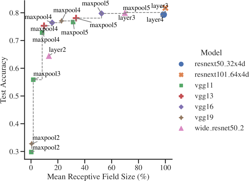
Figure B5: Our approach, PixPNet, evaluation on CUB-200-2011 with various backbones discovered by the ImageNette proxy approach outlined in the main text. The Pareto front is given by the dashed line.

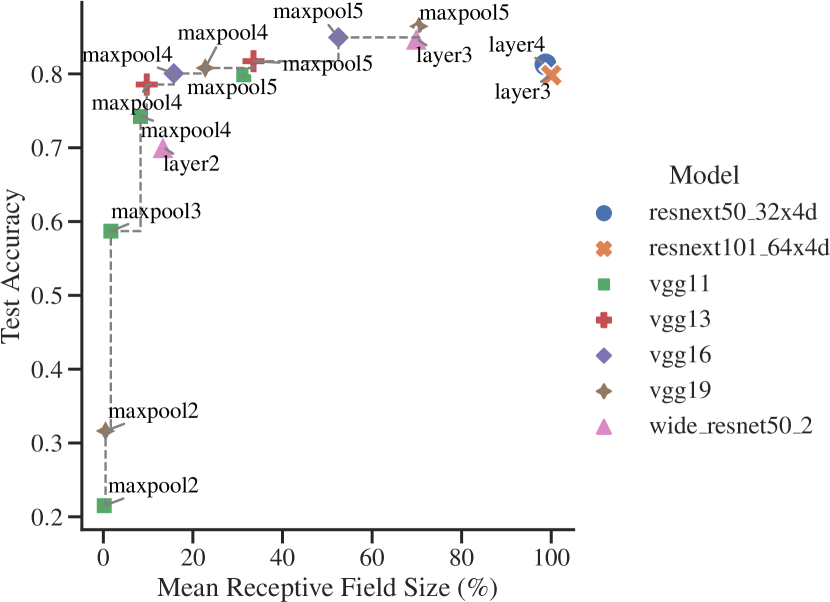
Figure B6: Our approach, PixPNet, evaluation on Stanford Cars with various backbones discovered by the ImageNette proxy approach outlined in the main text. The Pareto front is given by the dashed line.

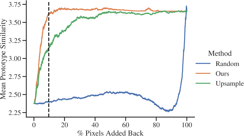
Figure B7: Relative ordering test for a VGG13@maxpool4. The original, random, and our pixel space mappings are compared. We achieve the highest AUSC and the lowest %2R. PRP is not shown because its implementation only supports ResNet models. The black dashed line indicates the mean receptive field of maxpool4.

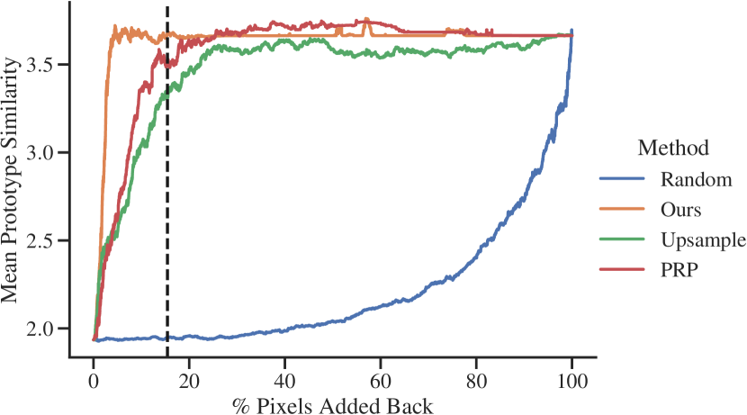
Figure B8: Relative ordering test for a ResNet18@layer2. The original, random, and our pixel space mappings are compared. We achieve the highest AUSC and the lowest %2R. The black dashed line indicates the mean receptive field of layer2.

BBox	D1	D2	D3	Model	$f$	Expl. Size $+$	Expl. Size $\pm$	$P$	MRF	Accuracy	$\pm$	Code Avail.	Val. Set
✗	✓	✓	✓	PixPNet	VGG19@maxpool5	10	10	2000	70.4	86.44	0.2	✓	✓
				PixPNet	VGG16@maxpool5	10	10	2000	52.5	84.94	0.1	✓	✓
				PixPNet	VGG13@maxpool5	10	10	2000	33.5	81.72	0.2	✓	✓
				PixPNet	VGG16@maxpool4	10	10	2000	15.8	80.05	0.3	✓	✓
	✓	✗	✓	Support ProtoPNet [86]	ResNet152	180	35280	17640	100	87.30	–	✗	?
				Deformable [20]	ResNet152	180	35280	17640	100	86.50	–	✓	✗
				ST-ProtoPNet [86]	ResNet152	20	3920	1960	100	85.30	–	✗	?
✓	✓	✗	✓	ST-ProtoPNet [86]	DenseNet161	20	3920	1960	100	92.70	0.2	✗	?
				TesNet [87]	DenseNet161	20	3920	1960	100	92.60	0.3	✓	✗
				ProtoPool [67]	ResNet34	20	390	195	100	89.30	0.1	✓	✗
				ProtoPNet [13]	VGG19	20	3920	1960	100	87.40	0.3	✓	✗
				ProtoTree [59]	ResNet34	22	390	195	100	86.60	0.2	✓	✗
				ProtoPShare [68]	ResNet34	960	960	480	100	86.38	–	✓	✗
				Proto2Proto [40]	ResNet18	20	3920	1960	100	84.00	–	✓	✗
✗	✗	✗	✗	ViT-NeT [42]	SwinT-B	12	126	63	100	95.00	–	✓	✗
	✗	✗	✓	ProtoPFormer [88]	CaiT-XXS-24	30	5880	2940	100	91.04	–	✓	✗

Table B5: ProtoPartNN results on Stanford Cars with ImageNet used for pre-training. Columns D1, D2, and D3 correspond to the three desiderata established in the main text. “BBox” indicates whether a method crops each image using a bounding box annotation. The best results of ProtoPartNNs with and without such annotations are bold and underlined, respectively. Best results that are within one standard deviation of each other are all emphasized. The table is split based on whether the method meets at least two desiderata.

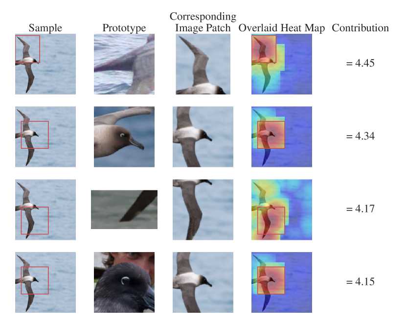
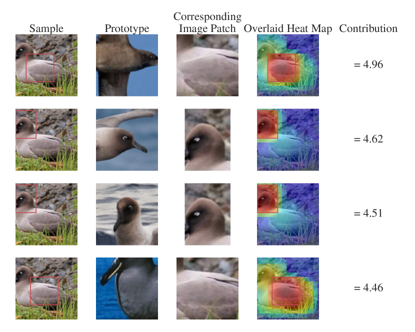
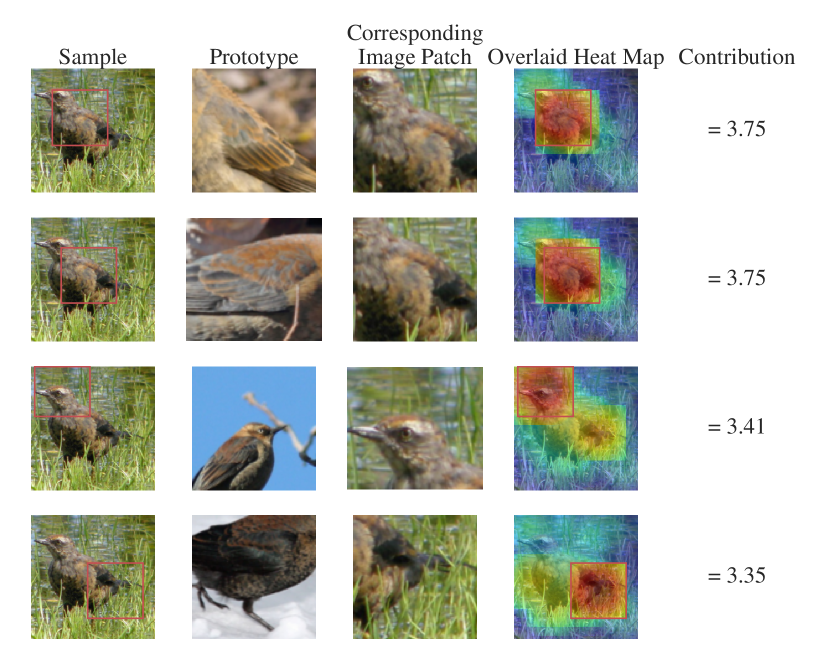
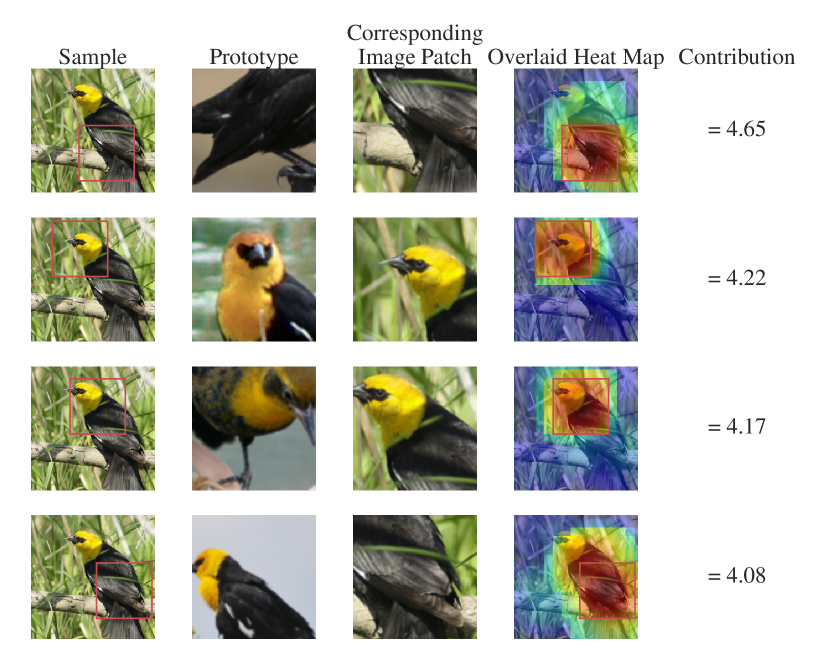
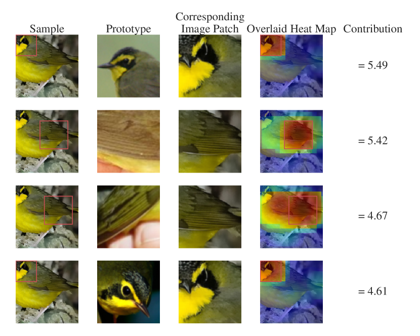
Figure B9: Examples of PixPNet explanations on CUB-200-2011.

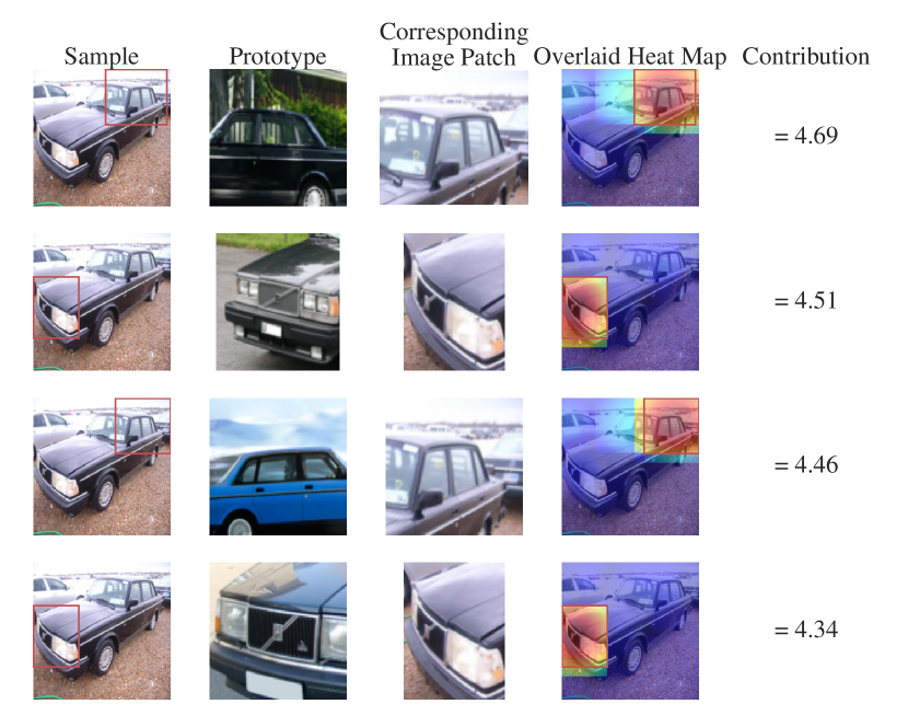
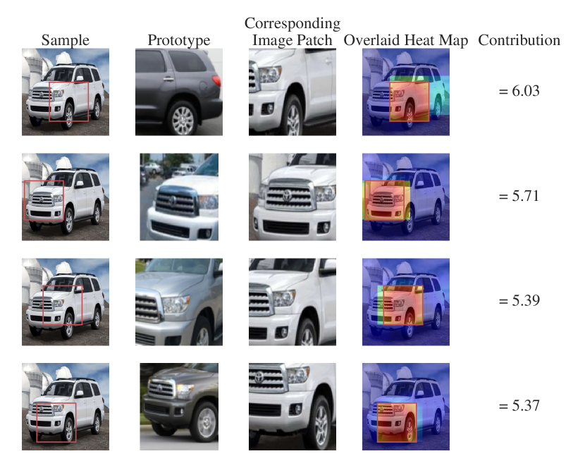
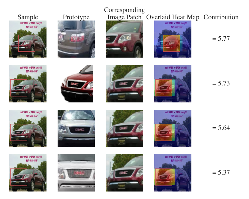
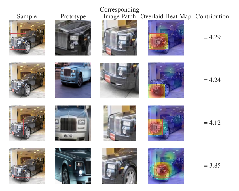
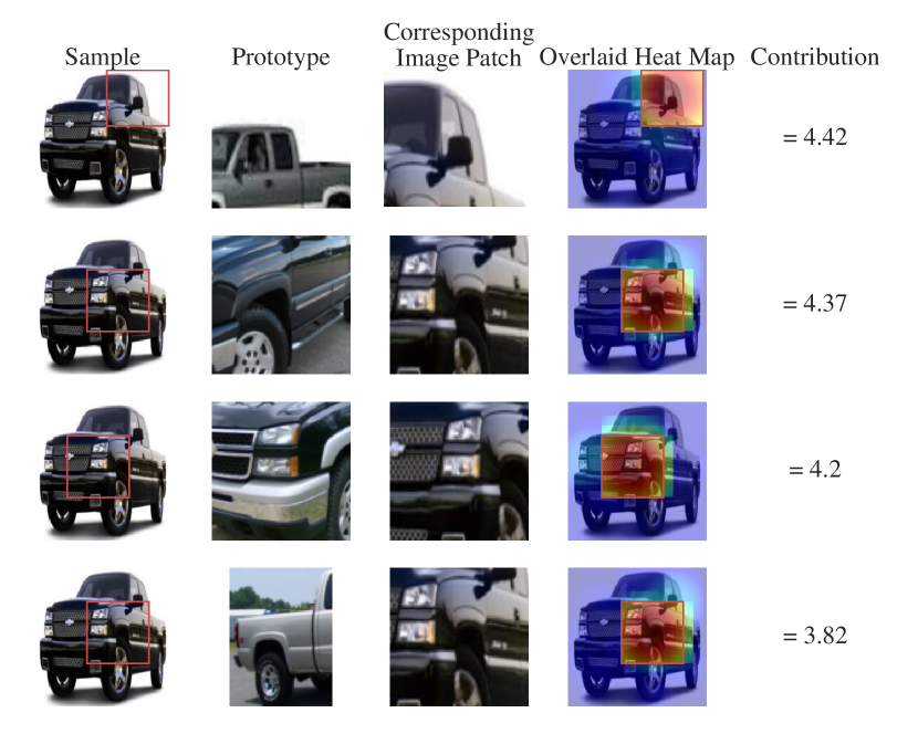
Figure B10: Examples of PixPNet explanations on Stanford Cars.

Appendix C Additional Receptive Field Algorithm Details

Here, we provide addition description of are function receptive field computation algorithm, FunctionalRF. Some complexity of the algorithm comes from handling arbitrary non-sequential architectures. FunctionalRF, takes a neural network as input and outputs the exact receptive field of every neuron in the neural network. Recall that a neuron is a function of a subset of pixels defined by its receptive field. FunctionalRF represents receptive fields as hypercubes (multidimensional tensor slices). For convolutional neural networks, we have four dimensions, but the batch size can safely be ignored. We use the notation $\llbracket a,b\rrbracket$ to denote the slice (discrete interval) between $a$ and $b$. The computation is outlined (see Algorithm 1) for image data for simplicity – the algorithm works for any number of dimensions or type of data. Given the directed acyclic computation graph of a neural network ${\mathcal{G}}$, we can traverse the topologically sorted graph node by node to satisfy input dependencies. At the start, we initialize the receptive field (rf attribute) of the input node $v_{0}\in{\mathcal{G}}$ as $1\times 1\times 1$ slices into the input image. Each consecutive node $v_{k}$ performs operation-dependent indexing into the receptive fields of its incoming nodes $\mathcal{U}_{k}$. This indexing is operation-dependent and is encapsulated by the function take_from$(\cdot)$. For instance, the slices for a 2D convolution with a $5{\times}5$ kernel, stride of 1, and $c_{\text{in}}$ channels at output position $3,3$ would be $\{\{\llbracket 1,c_{\text{in}}\rrbracket,\llbracket 1,5\rrbracket,\llbracket 1,5\rrbracket\}\}$ where $\llbracket a,b\rrbracket$ denotes the slice between $a$ and $b$. After, we merge (merge$(\cdot)$) as many hypercubes as possible into a larger hypercube (consider, e.g., one hypercube inside of another) to greatly reduce the space and time complexities. Figure C11 gives several examples of this merge operation. Finally, the receptive field-augmented graph ${\mathcal{G}}$ is returned.

Figure C11: Examples of index merging with 2D slices. Slices that cannot be merged are retained as a set.

Input: ${\mathcal{G}}$, the computation graph

Output: ${\mathcal{G}}$, augmented with receptive field information

1 Topologically sort ${\mathcal{G}}$;

// Initialize each input node rf element as a $1{\times}1{\times}1$ hypercube

2 $v_{0}.\texttt{rf}_{dij}\leftarrow\{\{\llbracket 1,3\rrbracket,\llbracket i,i\rrbracket,\llbracket j,j\rrbracket\}\}$;

3 for $v_{k}\in{\mathcal{G}}$ do

4       $\mathcal{U}_{k}\leftarrow$ all incoming nodes of $v_{k}$;

       // Record slicing operations of $v_{k}$

5       $v_{k}.\texttt{rf}_{dij}\leftarrow v_{k}.\texttt{take\_from}(\{u_{k}.\texttt{rf}\mid u_{k}\in\mathcal{U}_{k}\})$;

       // Merge hypercubes

6       $v_{k}.\texttt{rf}_{dij}\leftarrow\texttt{merge}(v_{k}.\texttt{rf}_{dij})$;

7      

return ${\mathcal{G}}$

Algorithm 1 FunctionalRF(${\mathcal{G}}$)

Appendix D Additional Pixel Space Mapping Algorithm Details

In order to compute a pixel space heat map, we propose an algorithm based on FunctionalRF rather than naively upsampling an embedding space similarity map ${{\bm{S}}}_{ij}$. Our approach uses the same idea as going from embedding space to pixel space. Each pixel space heat map ${\bm{M}}_{ij}\in{\mathbb{R}}^{H\times W}$ is initialized to all zeros ($\mathbf{0}^{H\times W}$), and corresponds to a sample ${{\bm{x}}}_{i}$ and a prototype ${{\bm{p}}}_{j}$. Let ${\bm{M}}_{ij}^{S}$ be the region of ${\bm{M}}_{ij}$ defined by the receptive field of similarity score ${S}\in{{\bm{S}}}_{ij}$. For each ${S}$, the pixel space heat map is updated as ${\bm{M}}_{ij}^{S}\leftarrow\max({\bm{M}}_{ij}^{S},{S})$ where $\max(\cdot)$ is an element-wise maximum that appropriately handles the case of overlapping receptive fields. Note that we weight ${S}$ by $T(|r_{i}|,|r_{j}|,\sigma_{T})$ (via broadcasting) where $T$ generates a 2D Gaussian kernel, $|\cdot|$ gives the length of a discrete interval, and $\sigma_{T}$ is the standard deviation of the kernel. The first two arguments denote the height and width of the kernel, respectively. We set $\sigma_{T}$ to the larger of the height and width. The intuition behind this approach is that a receptive field is actually Gaussian [52] – pixels in the center are more important, and pixels at the periphery are less important. We stress that this does not affect localization and the pixel space heat maps are largely unchanged without this step. However, this does affect the relevance order testing – without this Gaussian weighting step, the pixels within a receptive field would all have the same value, so the most important pixel in the region is selected arbitrarily. Selecting in the center and “spiraling” outwards is more faithful to what is known about deep neural networks [52]. In experiments, we also confirm that this step improves the relevance ordering test scores, especially in the case of large receptive fields. The full procedure (RFPixelSpaceMapping) is shown in Algorithm 2.

Input: $v_{k}$, the embedding layer in ${\mathcal{G}}$ (augmented by Algorithm 1)

Input: ${{\bm{S}}}$, the similarity map for a prototype

Output: ${\bm{M}}$, a pixel space heat map

1 ${\bm{M}}\leftarrow$ matrix of zeros $\in{\mathbb{R}}^{H\times W}$;

2 for rf${}_{dij}\in v_{k}.\texttt{{rf}}$ do

3       for $(r_{d},r_{i},r_{j})\in\texttt{{rf}}_{dij}$ do

4             ${\bm{M}}_{r_{d}r_{i}r_{j}}\leftarrow\textup{max}({{\bm{S}}}_{dij}\times T(|r_{i}|,|r_{j}|,\sigma_{T}),{\bm{M}}_{r_{d}r_{i}r_{j}})$;

5            

6      

return ${\bm{M}}$

Algorithm 2 RFPixelSpaceMapping($v_{k}$, ${{\bm{S}}}$)

Appendix E Experiment Setup and Reproducibility

Hardware and Software

The code for this paper was implemented in Python and primarily relies on PyTorch [61] and PyTorch Lightning [24]. The original ProtoPNet [13] code was used to guide some development, but the majority of code deviated (especially the training code which actually uses a validation split for validation and tuning). All experiments were run on NVIDIA A10 GPUs. Unless stated elsewhere, all experimental results are reported as the average across 10 trials. Our code will be made fully available upon publication.

Data Augmentation

For the CUB-200-2011 and Stanford Cars datasets, we perform the following augmentations to each training image:

1. Resize smallest dimension of image to 510 pixels with bilinear interpolation

2. Gaussian blur with 5 $\times$ 5 kernel and random sigma in the range $[0.1,5]$ (1/10 probability)

3. Randomly adjust sharpness by a factor of 1.5 (1/10 probability)

4. Randomly rotate image in the range $[-15,15]$ degrees (1/3 probability)

5. Randomly distort the image perspective with a scale of 0.2 (1/3 probability)

6. Randomly shear the image by 10 degrees (1/3 probability)

7. Randomly flip the image horizontally (1/2 probability)

8. Randomly crop the image to 384 $\times$ 384 pixels

9. Downsample the image to 224 $\times$ 224 pixels with bilinear interpolation

10. Normalize the image to have the channel-wise mean and standard deviation of the full data set

For ImageNette, steps 1 and 9 are omitted, and the random crop is done to 224 $\times$ 224 pixels directly.

We use an augmentation factor which indicates how many augmented samples are generated for each training image. In ProtoPNet, 30 augmentations are generated for each sample. In addition, ProtoPNet uses offline (static) augmentation, whereas we use online augmentation.

Training

The training procedure largely follows that of ProtoPNet. For a warm-up period, we train just the add-on layers ${f_{\text{add}}}$ and the prototypes ${{\bm{P}}}$. Thereafter, all layers are trained. We use an exponential warm-up of the learning rate and use a cosine annealing learning rate scheduler (without restarts) [51]. Every $k$ epochs, we perform the prototype replacement procedure.

Hyperparameters

All hyperparameters are listed in the proceeding table.

Name	Value
Augmentation Factor	16
Validation Set Proportion	0.1
Pre-training	ImageNet
${\lambda_{\text{cls}}}$	0
${\lambda_{\text{sep}}}$	0
${\varphi}$	Cosine Distance
$\varepsilon$	$10^{-6}$
$P$	$C\times 10$
$D$	192
$H_{p}$	1
$W_{p}$	1
Learning Rate (${f_{\text{core}}}$ parameters)	0.0001
Learning Rate (${f_{\text{add}}}$ parameters)	0.003
Learning Rate (${{\bm{P}}}$)	0.003
Warm-Up Epochs	5
Learning Rate Scheduler (Warm-Up)	Exponential
Learning Rate Scheduler	Cosine
Weight Decay (All Parameters Except ${{\bm{P}}}$)	0.001
Optimizer	Adam
Batch Size	64
Epochs	20
Prototype Replacement	Every 4 Epochs

Table E6: Table of PixPNet hyperparameters used in experiments.

Appendix F “Goldilocks” Zone Experimental Details

For this experiment, we follow the same training procedure as for PixPNet, except for any ProtoPartNN-specific training (e.g., prototype replacement). See the previous section for data augmentation details. We select pre-packaged and ImageNet pre-trained architectures from PyTorch [61] to evaluate the intermediate layers of. Recall that the goal of this experiment is to discover backbones suitable for PixPNet by observing the Pareto front of the mean receptive field and accuracy on ImageNette [25]. See the main text for discussion about this data set and justification for this approach. For each selected intermediate layer, the network is dissected at that point and a new classification head is appended which comprises a $1\times 1$ 2D adaptive average pooling layer, a flattening of the unary dimensions, and a fully-connected layer. The training procedure is carried out for 10 epochs with a batch size of 32. The proceeding table outlines the selected architectures and intermediate layers that are evaluated.

Architecture	Intermediate Layers
densenet121	conv0,norm0,relu0,pool0,denseblock1, transition1,denseblock2,transition2, denseblock3,transition3,denseblock4,norm5, avgpool,classifier
densenet161
densenet169
densenet201
inception_v3	Conv2d_1a_3x3, Conv2d_2a_3x3,Conv2d_2b_3x3,maxpool1, Conv2d_3b_1x1,Conv2d_4a_3x3,maxpool2, Mixed_5b,Mixed_5c,Mixed_5d,Mixed_6a, Mixed_6b,Mixed_6c,Mixed_6d,Mixed_6e, Mixed_7c,avgpool,fc
resnet18	conv1,maxpool,layer1,layer2,layer3,layer4, avgpool,fc
resnet34
resnet50
resnet101
resnet152
resnext101_32x8d
resnext101_64x4d
resnext50_32x4d
wide_resnet50_2
wide_resnet101_2
squeezenet1_0	conv1,maxpool1,maxpool2,maxpool3, features,final_conv
squeezenet1_1
vgg11	conv1,maxpool1,maxpool2,maxpool3, maxpool4,maxpool5,avgpool,classifier
vgg13
vgg16
vgg19

Table F7: All evaluated intermediate layers of backbone candidate architectures.

Appendix G Similarity Function Formulation

We reduce numerical error of the original similarity function by reformulating it as:

$${v}(d)=\underbrace{\log\left(\frac{d+1}{d+\varepsilon}\right)}_{\text{Original formulation}}=\underbrace{\log\left(\frac{1}{d+\varepsilon}+1\right)}_{\text{New formulation}}.$$ (5)

To validate its accuracy, we compare its scores across various values to the expected similarity scores with infinite precision. We use the mpmath [56] library to implement infinite precision. The table below compares the mean-squared-error of our approach to the original and our version of the similarity function. Our reformulation achieves lower error, especially in the $[1,10]$ value range for both 32- and 64-bit IEEE 754 floating point numbers.

Dtype	Region	MSE		% Improved
		Original	Ours
Float32	0, 1e-6	1.05e-13	1.04e-13	1.11%
	1e-6, 1e-3	4.08e-14	3.97e-14	2.69%
	1e-3, 1	3.56e-15	3.30e-15	7.41%
	1, 10	1.42e-15	1.03e-15	27.13%
	10, 1000	1.19e-15	1.18e-15	0.90%
Float64	0, 1e-6	3.61e-31	3.56e-31	1.14%
	1e-6, 1e-3	1.40e-31	1.35e-31	3.09%
	1e-3, 1	1.16e-32	1.05e-32	9.12%
	1, 10	4.63e-33	3.27e-33	29.28%
	10, 1000	4.12e-33	4.09e-33	0.65%

Table G8: The comparative numerical error of the similarity functions: original and ours. Mean-squared-error (MSE) is shown for IEEE 754 floating point data types. Our reformulation is more accurate especially in the $[1,10]$ range of values.

Appendix H Issues with ProtoPNet Code Base

Upon inspection of the original code base, we discovered that the test set accuracy is used to influence training of ProtoPNet. In fact, neither ProtoPNet nor its extensions for image classification that are mentioned in the paper employ a validation set in provided implementations. Part of this is due to some code bases being derived from the original implementation. ProtoPNet peeked at test set, which propagated to subsequent paper implementations. According to their implementation, they did not only have no validation set, In addition, the provided code also used the accuracy on the test set to influence when training should stop.

The relevant portions of code are shown below. In main.py, there is a training loop that saves the model twice each epoch (once before prototype replacement and once after). Each time that the model is saved, the accuracy on the test set is stored with the model. In addition, if the test accuracy is above 70%, then a message is logged to the console stating that the test accuracy is above said target.

Listing 1: main.py Snippet

⬇

172accu = tnt.test(model=ppnet_multi, dataloader=test_loader,

173 class_specific=class_specific, log=log)

174save.save_model_w_condition(model=ppnet, model_dir=model_dir, model_name=str(epoch) + ’push’, accu=accu,

175 target_accu=0.70, log=log)

The save module is from the save.py. The relevant snippet is shown below.

Listing 2: save.py Snippet

⬇

4def save_model_w_condition(model, model_dir, model_name, accu, target_accu, log=print):

5 ”’

6␣␣␣␣model:␣this␣is␣not␣the␣multigpu␣model

7␣␣␣␣’”

8 if accu > target_accu:

9 log(’\tabove␣{0:.2f}%’.format(target_accu * 100))

10 # torch.save(obj=model.state_dict(), f=os.path.join(model_dir, (model_name + ’{0:.4f}.pth’).format(accu)))

11 torch.save(obj=model, f=os.path.join(model_dir, (model_name + ’{0:.4f}.pth’).format(accu)))

The purpose of the held-out test set is to properly measure generalization error, not be used to tune hyperparameters nor influence training. Doing so is actually overfitting the distribution of the test set rather than truly improving performance. This phenomenon unfortunately has been long-standing in deep learning research, affecting progress with prominent datasets, including CIFAR-10 and ImageNet [65, 64, 32]. In our implementation, we employ a proper validation set and tune hyperparameters only according to accuracy on this split. This ensures that we are properly measuring generalization error.

In addition, we were able to approach but not reproduce the originally reported accuracies, nor could some others, using the provided code and instructions.

Appendix I Full Discussion of ProtoPNet Variants and Extensions

The idea of sharing prototypes between classes has been explored in ProtoPShare [68] (prototype merge-pruning) and ProtoPool [67] (differential prototype assignment). In ProtoTree [59], the classification head is replaced by a differentiable tree, also with shared prototypes. A procedure is also proposed to convert to a hard tree to improve interpretability. An alternative embedding space is explored in TesNet [87] based on Grassmann manifolds. The authors additionally propose a new similarity function, an orthogonality loss, and a subspace loss. A ProtoPartNN-specific knowledge distillation approach is proposed in Proto2Proto [40] by enforcing that student prototypes and embeddings should be close to those of the teacher. Deformable ProtoPNet [20] extends the ProtoPNet architecture with deformable prototypes. ST-ProtoPNet [86] learns support prototypes that lie near the classification boundary and trivial prototypes that are far from the classification boundary.

Figure I12: Proposed desiderata of ProtoPartNNs: part localization, linear/simple-tree case-based reasoning, and prototypes are image patches. Architectures at the intersection of all three desiderata are considered true ProtoPartNNs. Only architectures for image classification tasks are shown.

ProtoPNet has also been extended for graphs. ProtGNN [89] is an adaptation for graph classification and is built on by PxGNN [14], which extends it for node classification. Simultaneously, GCN-{TesNet,ProtoPNet} [62] was also proposed for graph and node classification. Likewise ProSeNet [55], extends the architecture for sequential data and ProtoSeg [70] can handle supervised image segmentation tasks. ProtoPNet has been adapted to task-specific applications, including EEG data (ProtoPMed-EEG [5]), Earth science data (ProtoLNet [4]), and deepfake detection (DPNet [83]). There have been a handful of ProtoPNet extensions tailored for diagnosing the chest CT scans of COVID-19 patients This includes Quasi-ProtoPNet [74] (removes non-class weight connections in $h$), NP-ProtoPNet [77] (fixes weights in $h$ to $+1$ and $-1$ for same- and non-class connections), Gen-ProtoPNet [75] (uses larger prototype kernel sizes), Ps-ProtoPNet [76] (combines Gen-ProtoPNet and NP-ProtoPNet), and XProtoNet [41] (prototypes are compared with dynamically-sized feature patches).

ProtoPartNN Tools   A few tools have also been proposed. In ProtoPDebug [6], a concept-level debugger for ProtoPNet is proposed in which a human supervisor, guided by model explanations, removes part-prototypes that have learned shortcuts or confounds. In [58], a methodology is developed to enhance ProtoPartNN explanations with color, hue, saturation, shape, texture, and contrast information.

In an attempt to improve ProtoPNet visualizations, an extension of layer-wise relevance propagation [2], Prototypical Relevance Propagation (PRP), is proposed to create more model-aware explanations [28]. PRP is quantitatively more effective in debugging erroneous prototypes and assigning pixel relevance than the original approach.

ProtoPartNN-Like Methods

The following papers are inspired by ProtoPNet but cannot be considered to be the same class of model. This is due to not fulfilling at least one of the proposed ProtoPartNN desiderata.

ViT-NeT [42] combines a vision transformer (ViT) with a neural tree decoder that learns prototypes. However, its training does not employ prototype pushing and has additional layers after the embedding layer that modify the embedding space. This breaks the mapping back to pixel space.

In another transformer-based approach, ProtoPFormer [88] exploits the inherent architectural features (local and global branches) of ViTs. The prototype layer has both local and global prototypes, and a focal loss concentrates local prototypes on heterogeneous regions of the foreground. However, the training procedure of the method removes prototype replacement.

Semi-ProtoPNet [80] fixes the readout weights as NP-ProtoPNet does and is applied to classification of defective structures in power distribution networks. However, the training procedure of the method also skips over prototype replacement.

In SDFA-SA-ProtoPNet [36], a shallow-deep feature alignment (SDFA) module aligns the similarity structures between deep and shallow layers. In addition, a score aggregation (SA) module aggregates similarity scores of prototypes in a class-wise manner to avoid learning inter-class information. Notably, the authors attempt to quantitatively evaluate the interpretability of prototype-based explanations rather than relying on qualitative examples as many other extensions have done. We discuss the proposed metrics in the main text. Once again, the training procedure omits prototype replacement.

Throughout each of these works, the main justification for removing prototype replacement is that it harms task accuracy.

ProtoVAE [27] is an extension of ProtoPNet for variational auto-encoders (VAEs). It outperforms ProtoPNet on a variety of classification tasks. It uses an orthogonality loss for intra-class diversity (same as TesNet). However, it does not employ prototype replacement, opting to rather use a decoder used to visualize prototypes.

Retrospective on Extensions

Despite all these efforts, all extensions still have fundamental issues with object part localization, pixel space grounding, and heat map visualizations. We discuss what these issues are in detail in the main text.

Appendix J Additional Consistency and Stability Details

For the CUB-200-2011 dataset, there are 15 object parts: back, beak, belly, breast, crown, forehead, left eye, left leg, left wing, nape, right eye, right leg, right wing, tail, and throat. However, we treat the left and right versions of an object as the same object as 1) semantically, they are the same object, 2) we do not want to penalize ProtoPartNNs for learning invariance to flips or rotations, and 3) data augmentation flips images, which makes lefts look like rights (and vice versa). In addition, owing to data preprocessing, some object parts are not visible in images that are visible in the uncropped image. Naturally, we do not penalize ProtoPartNNs for not matching with parts that are not visible.

Limitations

The consistency and stability metrics ignore the localization capability of ProtoPartNNs and arbitrarily set the localization window to 72 $\times$ 72 pixels, centered around the localization bounding box midpoint. In addition, the threshold of 0.8 is arbitrary for a prototype to be consistent. We argue that a soft score (the average of the prototype-object coinciding frequencies without thresholding) makes far more sense. It can be interpreted as the average consistency of all prototypes, rather than the proportion of prototypes that are at least 80% consistent. When computing these soft scores, we noticed that the majority of them were in the $[0.6,0.8]$ range. Last, the metric relies on human object part annotations – in the case of CUB-200-2011, all annotations are of bird parts. However, it is well-known that prototypes learn backgrounds and other foreground objects that are also discriminatory (such as oceans, tree branches, and human hands) [78, 43]. Prototypes may be consistent (and stable), but associated with the wrong part of the image just because of the 1) limited part annotations, and 2) the arbitrary 72 $\times$ 72 pixel window. Nonetheless, the metrics do allow for comparative interpretability evaluation between ProtoPartNNs. Further information on the consistency and stability metrics is available in our code implementation as well as [36].

Appendix K Additional Small Improvements

We noticed that the magnitude of feature maps always dictates prototype similarity when using Euclidean distance. Using cosine distance eliminates the influence of magnitude on prototype similarity.

In ProtoPNet, the incorrect gain and initialization method is used in the initialization of the convolutional weights in ${f_{\text{add}}}$ before the sigmoid activation. The original implementation uses a Kaiming normal initialization with a gain that is intended for the ReLU activation. Instead, we use the Xavier normal initialization with a gain of one.

References

- [1] André Araujo, Wade Norris, and Jack Sim. Computing receptive fields of convolutional neural networks. Distill, 2019. https://distill.pub/2019/computing-receptive-fields.
- [2] Sebastian Bach, Alexander Binder, Grégoire Montavon, Frederick Klauschen, Klaus-Robert Müller, and Wojciech Samek. On pixel-wise explanations for non-linear classifier decisions by layer-wise relevance propagation. PloS one, 10(7):e0130140, 2015.
- [3] Hubert Baniecki. Adversarial explainable AI. https://hbaniecki.com/adversarial-explainable-ai/, 2023. Accessed: 2023-01-28.
- [4] Elizabeth A. Barnes, Randal J. Barnes, Zane K. Martin, and Jamin K. Rader. This looks like that there: Interpretable neural networks for image tasks when location matters. Artificial Intelligence for the Earth Systems, 1(3):e220001, 2022.
- [5] Alina Jade Barnett, Zhicheng Guo, Jin Jing, Wendong Ge, Cynthia Rudin, and M. Brandon Westover. Mapping the ictal-interictal-injury continuum using interpretable machine learning. arXiv, 2022.
- [6] Andrea Bontempelli, Stefano Teso, Fausto Giunchiglia, and Andrea Passerini. Concept-level debugging of part-prototype networks. In International Conference on Learning Representations, ICLR. OpenReview, 2023.
- [7] Sebastian Bordt, Michèle Finck, Eric Raidl, and Ulrike von Luxburg. Post-hoc explanations fail to achieve their purpose in adversarial contexts. ACM Conference on Fairness, Accountability, and Transparency, 5, 2022.
- [8] Joy Buolamwini and Timnit Gebru. Gender Shades: Intersectional Accuracy Disparities in Commercial Gender Classification. In Conference on Fairness, Accountability and Transparency, pages 77–91. PMLR, Jan. 2018.
- [9] Oana-Maria Camburu, Eleonora Giunchiglia, Jakob Foerster, Thomas Lukasiewicz, and Phil Blunsom. Can i trust the explainer? verifying post-hoc explanatory methods. In NeurIPS 2019 Workshop on Safety and Robustness in Decision Making. arXiv, 2019.
- [10] Zachariah Carmichael and Walter J. Scheirer. A framework for evaluating post hoc feature-additive explainers. arXiv, abs/2106.08376, 2021.
- [11] Zachariah Carmichael and Walter J Scheirer. Unfooling perturbation-based post hoc explainers. In Proceedings of the AAAI Conference on Artificial Intelligence. AAAI, 2023.
- [12] Selina Carter and Jonathan Hersh. Explainable ai helps bridge the ai skills gap: Evidence from a large bank. Economics Faculty Articles and Research, 276, 2022.
- [13] Chaofan Chen, Oscar Li, Daniel Tao, Alina Barnett, Cynthia Rudin, and Jonathan Su. This looks like that: Deep learning for interpretable image recognition. In Hanna M. Wallach, Hugo Larochelle, Alina Beygelzimer, Florence d’Alché-Buc, Emily B. Fox, and Roman Garnett, editors, Neural Information Processing Systems, NeurIPS, pages 8928–8939, 2019.
- [14] Enyan Dai and Suhang Wang. Towards prototype-based self-explainable graph neural network. arXiv, 2022.
- [15] Guy Van den Broeck, Anton Lykov, Maximilian Schleich, and Dan Suciu. On the tractability of SHAP explanations. In AAAI Conference on Innovative Applications of Artificial Intelligence, IAAI, pages 6505–6513. AAAI Press, 2021.
- [16] Jia Deng, Wei Dong, Richard Socher, Li-Jia Li, Kai Li, and Li Fei-Fei. Imagenet: A large-scale hierarchical image database. In IEEE Computer Society Conference on Computer Vision and Pattern Recognition, pages 248–255. IEEE Computer Society, 2009.
- [17] Botty Dimanov, Umang Bhatt, Mateja Jamnik, and Adrian Weller. You shouldn’t trust me: Learning models which conceal unfairness from multiple explanation methods. Frontiers in Artificial Intelligence and Applications: ECAI, 2020.
- [18] Ann-Kathrin Dombrowski, Maximillian Alber, Christopher Anders, Marcel Ackermann, Klaus-Robert Müller, and Pan Kessel. Explanations can be manipulated and geometry is to blame. Advances in neural information processing systems, 32, 2019.
- [19] Xuanyi Dong and Yi Yang. Nas-bench-201: Extending the scope of reproducible neural architecture search. In International Conference on Learning Representations, ICLR. OpenReview.net, 2020.
- [20] Jon Donnelly, Alina Jade Barnett, and Chaofan Chen. Deformable ProtoPNet: An interpretable image classifier using deformable prototypes. In Conference on Computer Vision and Pattern Recognition, CVPR, pages 10255–10265. IEEE/CVF, 2022.
- [21] Finale Doshi-Velez and Been Kim. Towards a rigorous science of interpretable machine learning. arXiv, 2017.
- [22] Council of the EU and European Parliament. Regulation (EU) 2016/679 of the European Parliament and of the Council of 27 April 2016 on the protection of natural persons with regard to the processing of personal data and on the free movement of such data, and repealing Directive 95/46/EC (General Data Protection Regulation). Official Journal of the European Union, L 119:1–88, 2016.
- [23] European Commission. Proposal for a regulation of the European Parliament and the Council: Laying down harmonised rules on Artificial Intelligence (Artificial Intelligence Act) and amending certain Union legislative acts. https://eur-lex.europa.eu/legal-content/EN/TXT/?uri=CELEX:52021PC0206, 4 2021.
- [24] William Falcon and The PyTorch Lightning team. PyTorch Lightning, 3 2019. https://github.com/Lightning-AI/lightning.
- [25] FastAI. Imagenette. https://github.com/fastai/imagenette, 2020.
- [26] Damien Garreau and Ulrike von Luxburg. Explaining the explainer: A first theoretical analysis of LIME. In Silvia Chiappa and Roberto Calandra, editors, International Conference on Artificial Intelligence and Statistics, volume 108 of Proceedings of Machine Learning Research, pages 1287–1296. PMLR, Aug. 2020.
- [27] Srishti Gautam, Ahcene Boubekki, Stine Hansen, Suaiba Amina Salahuddin, Robert Jenssen, Marina M.-C. Höhne, and Michael Kampffmeyer. ProtoVAE: A trustworthy self-explainable prototypical variational model. In Neural Information Processing Systems, NeurIPS, 2022.
- [28] Srishti Gautam, Marina M.-C. Höhne, Stine Hansen, Robert Jenssen, and Michael Kampffmeyer. This looks more like that: Enhancing self-explaining models by prototypical relevance propagation. Pattern Recognition, 136:1–13, 2023.
- [29] Kamaledin Ghiasi-Shirazi. Generalizing the convolution operator in convolutional neural networks. Neural Processing Letters, 50(3):2627–2646, 2019.
- [30] Kaiming He, Xiangyu Zhang, Shaoqing Ren, and Jian Sun. Deep residual learning for image recognition. In IEEE Conference on Computer Vision and Pattern Recognition, CVPR, pages 770–778. IEEE Computer Society, 2016.
- [31] Dan Hendrycks, Kevin Zhao, Steven Basart, Jacob Steinhardt, and Dawn Song. Natural adversarial examples. In Conference on Computer Vision and Pattern Recognition, pages 15262–15271. IEEE/Computer Vision Foundation, 2021.
- [32] Dan Hendrycks, Kevin Zhao, Steven Basart, Jacob Steinhardt, and Dawn Song. Natural adversarial examples. In Proceedings of the IEEE/CVF Conference on Computer Vision and Pattern Recognition, pages 15262–15271, 2021.
- [33] Robin Hesse, Simone Schaub-Meyer, and Stefan Roth. FunnyBirds: A synthetic vision dataset for a part-based analysis of explainable AI methods. In IEEE/CVF International Conference on Computer Vision, ICCV, pages 1–18. IEEE, 2023.
- [34] Adrian Hoffmann, Claudio Fanconi, Rahul Rade, and Jonas Kohler. This looks like that… does it? Shortcomings of latent space prototype interpretability in deep networks. In ICML Workshop on Theoretic Foundation, Criticism, and Application Trend of Explainable AI, 2022.
- [35] Gao Huang, Zhuang Liu, Laurens van der Maaten, and Kilian Q. Weinberger. Densely connected convolutional networks. In IEEE Conference on Computer Vision and Pattern Recognition, CVPR, pages 2261–2269. IEEE Computer Society, 2017.
- [36] Qihan Huang, Mengqi Xue, Haofei Zhang, Jie Song, and Mingli Song. Is ProtoPNet really explainable? evaluating and improving the interpretability of prototypes. arXiv, 2022.
- [37] Christina Humer, Andreas Hinterreiter, Benedikt Leichtmann, Martina Mara, and Marc Streit. Comparing effects of attribution-based, example-based, and feature-based explanation methods on ai-assisted decision-making. OSF Preprints, 2022.
- [38] Sérgio Jesus, Catarina Belém, Vladimir Balayan, João Bento, Pedro Saleiro, Pedro Bizarro, and João Gama. How can i choose an explainer? an application-grounded evaluation of post-hoc explanations. In Proceedings of the ACM Conference on Fairness, Accountability, and Transparency, FAccT’21, page 805–815, New York, NY, USA, 2021. Association for Computing Machinery.
- [39] Harmanpreet Kaur, Harsha Nori, Samuel Jenkins, Rich Caruana, Hanna Wallach, and Jennifer Wortman Vaughan. Interpreting interpretability: Understanding data scientists’ use of interpretability tools for machine learning. In Regina Bernhaupt, Florian ’Floyd’ Mueller, David Verweij, Josh Andres, Joanna McGrenere, Andy Cockburn, Ignacio Avellino, Alix Goguey, Pernille Bjøn, Shengdong Zhao, Briane Paul Samson, and Rafal Kocielnik, editors, Conference on Human Factors in Computing Systems, pages 1–14. ACM, Apr. 2020.
- [40] Monish Keswani, Sriranjani Ramakrishnan, Nishant Reddy, and Vineeth N. Balasubramanian. Proto2Proto: Can you recognize the car, the way I do? In Conference on Computer Vision and Pattern Recognition, CVPR, pages 10223–10233. IEEE/CVF, 2022.
- [41] Eunji Kim, Siwon Kim, Minji Seo, and Sungroh Yoon. XProtoNet: Diagnosis in chest radiography with global and local explanations. In Conference on Computer Vision and Pattern Recognition, CVPR, pages 15719–15728. CVF/IEEE, 2021.
- [42] Sangwon Kim, Jae-Yeal Nam, and ByoungChul Ko. Vit-net: Interpretable vision transformers with neural tree decoder. In Kamalika Chaudhuri, Stefanie Jegelka, Le Song, Csaba Szepesvári, Gang Niu, and Sivan Sabato, editors, International Conference on Machine Learning, ICML, volume 162 of Proceedings of Machine Learning Research, pages 11162–11172. PMLR, 2022.
- [43] Sunnie S. Y. Kim, Nicole Meister, Vikram V. Ramaswamy, Ruth Fong, and Olga Russakovsky. HIVE: evaluating the human interpretability of visual explanations. In Shai Avidan, Gabriel J. Brostow, Moustapha Cissé, Giovanni Maria Farinella, and Tal Hassner, editors, European Conference on Computer Vision, ECCV, volume 13672 of Lecture Notes in Computer Science, pages 280–298. Springer, 2022.
- [44] Simon Kornblith, Jonathon Shlens, and Quoc V. Le. Do better imagenet models transfer better? In IEEE Conference on Computer Vision and Pattern Recognition, CVPR 2019, Long Beach, CA, USA, June 16-20, 2019, pages 2661–2671. Computer Vision Foundation / IEEE, 2019.
- [45] Khaled Koutini, Hamid Eghbal-zadeh, Matthias Dorfer, and Gerhard Widmer. The receptive field as a regularizer in deep convolutional neural networks for acoustic scene classification. In 27th European Signal Processing Conference, EUSIPCO 2019, A Coruña, Spain, September 2-6, 2019, pages 1–5. IEEE, 2019.
- [46] Jonathan Krause, Michael Stark, Jia Deng, and Li Fei-Fei. 3D object representations for fine-grained categorization. In 4th International IEEE Workshop on 3D Representation and Recognition (3dRR-13), Sydney, Australia, 2013.
- [47] Satyapriya Krishna, Tessa Han, Alex Gu, Javin Pombra, Shahin Jabbari, Steven Wu, and Himabindu Lakkaraju. The disagreement problem in explainable machine learning: A practitioner’s perspective. arXiv, pages 1–46, 2022.
- [48] Matthew L. Leavitt and Ari Morcos. Towards falsifiable interpretability research. In NeurIPS Workshop on ML-Retrospectives, Surveys & Meta-Analyses, pages 1–15. arXiv, 2020.
- [49] Library of Congress. H.R.6580 - 117th Congress (2021-2022): Algorithmic accountability act of 2022. https://www.congress.gov/bill/117th-congress/house-bill/6580/text, 2 2022.
- [50] Zachary C. Lipton. The mythos of model interpretability. ACM Queue, 16(3):30, July 2018.
- [51] Ilya Loshchilov and Frank Hutter. SGDR: Stochastic gradient descent with warm restarts. arXiv, 2016.
- [52] Wenjie Luo, Yujia Li, Raquel Urtasun, and Richard S. Zemel. Understanding the effective receptive field in deep convolutional neural networks. In Daniel D. Lee, Masashi Sugiyama, Ulrike von Luxburg, Isabelle Guyon, and Roman Garnett, editors, Advances in Neural Information Processing Systems 29: Annual Conference on Neural Information Processing Systems 2016, December 5-10, 2016, Barcelona, Spain, pages 4898–4906, 2016.
- [53] Sean McGregor. Preventing repeated real world AI failures by cataloging incidents: The AI incident database. In AAAI Conference on Innovative Applications of Artificial Intelligence, IAAI, pages 15458–15463. AAAI Press, 2021.
- [54] D. Douglas Miller and Eric W. Brown. Artificial intelligence in medical practice: The question to the answer? The American Journal of Medicine, 131(2):129–133, 2018.
- [55] Yao Ming, Panpan Xu, Huamin Qu, and Liu Ren. Interpretable and steerable sequence learning via prototypes. In Ankur Teredesai, Vipin Kumar, Ying Li, Rómer Rosales, Evimaria Terzi, and George Karypis, editors, SIGKDD International Conference on Knowledge Discovery & Data Mining, KDD, pages 903–913. ACM, 2019.
- [56] mpmath Contributors. Mpmath: A python library for arbitrary-precision floating-point arithmetic, 2022. https://github.com/mpmath/mpmath.
- [57] Keivan Nalaie, Kamaledin Ghiasi-Shirazi, and Modhammad-R. Akbarzadeh-T. Efficient implementation of a generalized convolutional neural networks based on weighted Euclidean distance. In International Conference on Computer and Knowledge Engineering, ICCKE, pages 211–216, 2017.
- [58] Meike Nauta, Annemarie Jutte, Jesper C. Provoost, and Christin Seifert. This looks like that, because… explaining prototypes for interpretable image recognition. In Machine Learning and Principles and Practice of Knowledge Discovery in Databases - International Workshops of ECML PKDD, volume 1524 of Communications in Computer and Information Science, pages 441–456. Springer, 2021.
- [59] Meike Nauta, Ron van Bree, and Christin Seifert. Neural prototype trees for interpretable fine-grained image recognition. In Conference on Computer Vision and Pattern Recognition, CVPR, pages 14933–14943. CVF/IEEE, 2021.
- [60] Cathy O’Neil. Weapons of Math Destruction: How Big Data Increases Inequality and Threatens Democracy. Crown, Sept. 2016.
- [61] Adam Paszke, Sam Gross, Francisco Massa, Adam Lerer, James Bradbury, Gregory Chanan, Trevor Killeen, Zeming Lin, Natalia Gimelshein, Luca Antiga, et al. Pytorch: An imperative style, high-performance deep learning library. Advances in neural information processing systems, 32, 2019.
- [62] Alessio Ragno, Biagio La Rosa, and Roberto Capobianco. Prototype-based interpretable graph neural networks. IEEE Transactions on Artificial Intelligence, pages 1–11, 2022.
- [63] Tim Räz. ML interpretability: Simple isn’t easy. arXiv, 2022.
- [64] Benjamin Recht, Rebecca Roelofs, Ludwig Schmidt, and Vaishaal Shankar. Do CIFAR-10 classifiers generalize to CIFAR-10? arXiv, 2018.
- [65] Benjamin Recht, Rebecca Roelofs, Ludwig Schmidt, and Vaishaal Shankar. Do ImageNet classifiers generalize to ImageNet? In International conference on machine learning, pages 5389–5400. PMLR, 2019.
- [66] Cynthia Rudin. Stop explaining black box machine learning models for high stakes decisions and use interpretable models instead. Nature Machine Intelligence, 1(5):206–215, May 2019.
- [67] Dawid Rymarczyk, Lukasz Struski, Michal Górszczak, Koryna Lewandowska, Jacek Tabor, and Bartosz Zielinski. Interpretable image classification with differentiable prototypes assignment. In Shai Avidan, Gabriel J. Brostow, Moustapha Cissé, Giovanni Maria Farinella, and Tal Hassner, editors, European Conference on Computer Vision, ECCV, volume 13672 of Lecture Notes in Computer Science, pages 351–368. Springer, 2022.
- [68] Dawid Rymarczyk, Lukasz Struski, Jacek Tabor, and Bartosz Zielinski. Protopshare: Prototypical parts sharing for similarity discovery in interpretable image classification. In Feida Zhu, Beng Chin Ooi, and Chunyan Miao, editors, SIGKDD Conference on Knowledge Discovery and Data Mining, KDD, pages 1420–1430. ACM, 2021.
- [69] Mikołaj Sacha, Bartosz Jura, Dawid Rymarczyk, Łukasz Struski, Jacek Tabor, and Bartosz Zieliński. Interpretability benchmark for evaluating spatial misalignment of prototypical parts explanations. arXiv, 2023.
- [70] Mikołaj Sacha, Dawid Rymarczyk, Łukasz Struski, Jacek Tabor, and Bartosz Zieliński. ProtoSeg: Interpretable semantic segmentation with prototypical parts. In Winter Conference on Applications of Computer Vision (WACV), pages 1481–1492. IEEE/CVF, January 2023.
- [71] Gesina Schwalbe and Bettina Finzel. A comprehensive taxonomy for explainable artificial intelligence: a systematic survey of surveys on methods and concepts. Data Mining and Knowledge Discovery, Jan 2023.
- [72] Joseph P. Simmons, Leif D. Nelson, and Uri Simonsohn. False-positive psychology: Undisclosed flexibility in data collection and analysis allows presenting anything as significant. Psychological Science, 22(11):1359–1366, 2011.
- [73] Karen Simonyan and Andrew Zisserman. Very deep convolutional networks for large-scale image recognition. In Yoshua Bengio and Yann LeCun, editors, International Conference on Learning Representations, ICLR, 2015.
- [74] Gurmail Singh. Think positive: An interpretable neural network for image recognition. Neural Networks, 151:178–189, 2022.
- [75] Gurmail Singh and Kin Choong Yow. An interpretable deep learning model for covid-19 detection with chest x-ray images. IEEE Access, 9:85198–85208, 2021.
- [76] Gurmail Singh and Kin-Choong Yow. Object or background: An interpretable deep learning model for COVID-19 detection from CT-scan images. Diagnostics, 11(9):1732, Sep 2021.
- [77] Gurmail Singh and Kin Choong Yow. These do not look like those: An interpretable deep learning model for image recognition. IEEE Access, 9:41482–41493, 2021.
- [78] Poulami Sinhamahapatra, Lena Heidemann, Maureen Monnet, and Karsten Roscher. Towards human-interpretable prototypes for visual assessment of image classification models. arXiv, 2022.
- [79] Dylan Slack, Sophie Hilgard, Emily Jia, Sameer Singh, and Himabindu Lakkaraju. Fooling LIME and SHAP: adversarial attacks on post hoc explanation methods. In Annette N. Markham, Julia Powles, Toby Walsh, and Anne L. Washington, editors, AAAI/ACM Conference on AI, Ethics, and Society (AIES), pages 180–186. ACM, 2020.
- [80] Stéfano Frizzo Stefenon, Gurmail Singh, Kin Choong Yow, and Alessandro Cimatti. Semi-ProtoPNet deep neural network for the classification of defective power grid distribution structures. Sensors, 22(13):4859, 2022.
- [81] Christian Szegedy, Wojciech Zaremba, Ilya Sutskever, Joan Bruna, Dumitru Erhan, Ian J. Goodfellow, and Rob Fergus. Intriguing properties of neural networks. In Yoshua Bengio and Yann LeCun, editors, International Conference on Learning Representations, pages 1–10, Apr. 2014.
- [82] Erico Tjoa and Cuntai Guan. A survey on explainable artificial intelligence (XAI): toward medical XAI. IEEE Transactions on Neural Networks and Learning Systems, 32(11):4793–4813, 2020.
- [83] Loc Trinh, Michael Tsang, Sirisha Rambhatla, and Yan Liu. Interpretable and trustworthy deepfake detection via dynamic prototypes. In Winter Conference on Applications of Computer Vision, WACV, pages 1972–1982. IEEE, 2021.
- [84] U.S.-EU TTC. U.S.-EU joint statement of the Trade and Technology Council. https://www.commerce.gov/news/press-releases/2022/05/us-eu-joint-statement-trade-and-technology-council, 5 2022.
- [85] Catherine Wah, Steve Branson, Peter Welinder, Pietro Perona, and Serge Belongie. The Caltech-UCSD Birds-200-2011 dataset. Technical Report CNS-TR-2011-001, California Institute of Technology, 2011.
- [86] Chong Wang, Yuyuan Liu, Yuanhong Chen, Fengbei Liu, Yu Tian, Davis J. McCarthy, Helen Frazer, and Gustavo Carneiro. Learning support and trivial prototypes for interpretable image classification. arXiv, 2023.
- [87] Jiaqi Wang, Huafeng Liu, Xinyue Wang, and Liping Jing. Interpretable image recognition by constructing transparent embedding space. In International Conference on Computer Vision, ICCV, pages 875–884. IEEE/CVF, 2021.
- [88] Mengqi Xue, Qihan Huang, Haofei Zhang, Lechao Cheng, Jie Song, Minghui Wu, and Mingli Song. ProtoPFormer: Concentrating on prototypical parts in vision transformers for interpretable image recognition. arXiv, 2022.
- [89] Zaixi Zhang, Qi Liu, Hao Wang, Chengqiang Lu, and Cheekong Lee. ProtGNN: Towards self-explaining graph neural networks. In Conference on Innovative Applications of Artificial Intelligence, IAAI, pages 9127–9135. AAAI Press, 2022.