Asymptotically optimal sequential anomaly identification with ordering sampling rules

Abstract

The problem of sequential anomaly detection and identification is considered in the presence of a sampling constraint. Specifically, multiple data streams are generated by distinct sources and the goal is to quickly identify those that exhibit “anomalous” behavior, when it is not possible to sample every source at each time instant. Thus, in addition to a stopping rule, which determines when to stop sampling, and a decision rule, which indicates which sources to identify as anomalous upon stopping, one needs to specify a sampling rule that determines which sources to sample at each time instant. The focus of this work is on ordering sampling rules, which sample the data sources, among those currently estimated as anomalous (resp. non-anomalous), for which the corresponding local test statistics have the smallest (resp. largest) values. It is shown that with an appropriate design, which is specified explicitly, an ordering sampling rule leads to the optimal expected time for stopping, among all policies that satisfy the same sampling and error constraints, to a first-order asymptotic approximation as the false positive and false negative error rates under control both go to zero. This is the first asymptotic optimality result for ordering sampling rules when multiple sources can be sampled per time instant. Moreover, this is established under a general setup where the number of anomalies is not required to be a priori known. A novel proof technique is introduced, which unifies different versions of the problem regarding the homogeneity of the sources and prior information on the number of anomalies.

,

1 Introduction

In many scientific and engineering problems with numerous data streams, it is important to be able to quickly identify those that exhibit outlying statistical behavior. For example, in navigation system integrity monitoring, it is critical to quickly identify a faulty sensor in order to remove it from the navigation system ([32, Section 11.1]) For rapid intrusion detection in computer networks, anomaly-based detection systems are trained to recognize standard network behavior, detect deviations from the standard profile in real time, and identify those deviations that can be classified as potential network attacks [33]. In brain science, it is desirable to identify groups of cells with large vibration frequency, as this might be a symptom of a developing malfunction [31].

Such applications motivate the study of sequential multiple testing problems in which (i) there are multiple data sequences generated by distinct data sources, (ii) two hypotheses are postulated for each of them, and (iii) the goal is to identify as quickly as possible those data streams in which the alternative hypotheses hold, and which are often interpreted as “anomalous”. In some formulations in the literature, each data stream can be observed continuously until a decision is reached for it (see, e.g., [3, 9, 29, 30, 4, 16]).

In others, a sampling constraint is imposed, according to which it is possible to sample only a fixed number of data sources at each time instant (see, e.g., [37, 8, 19, 14, 17, 36, 34, 12, 13, 28]). The latter problem can also be formulated as a sequential multi-hypothesis testing in which at each time instant there is a set of possible actions, i.e., the choice of the sources to be sampled, that can influence the distribution of the observations. Thus, methods and results from the literature of sequential design of experiments, or sequential multi-hypothesis testing with controlled sensing [7, 1, 5, 6, 23, 22, 24, 26, 27, 10] are, in principle at least, applicable as well.

A weaker sampling constraint for the problem of sequential anomaly identification was proposed recently in [35], according to which the number of sampled sources per time instant is not necessarily fixed. In the same work it was shown that, when using the stopping and decision rules proposed in [29] in the full sampling case, the optimal expected time for stopping is achieved asymptotically if the long-run sampling frequency of each source is not smaller than a critical value, which depends on the unknown subset of anomalous sources. Moreover, this criterion was shown to be satisfied, simultaneously for every possible subset of anomalous sources, by a probabilistic sampling rule, according to which each source is sampled at each time instant with a probability that depends on the current estimate of the subset of anomalous sources.

The focus of the present paper is on a different sampling approach that goes back at least to [7, Remark 5]. According to it, the choice of the sampled sources at each time instant is determined by the current order of the test statistics that correspond to the individual sources. Such a sampling rule, to which we refer as ordering, prioritizes sampling from sources that have not yet provided strong evidence for the testing problem, thus, it can be more efficient than the corresponding probabilistic sampling rule. This intuition has been confirmed by various simulation studies in the literature (see e.g., [8, 19, 36]). However, theoretical support for ordering sampling rules has been relatively limited and restricted to specific setups. Specifically, a second-order asymptotic optimality analysis has been conducted in [24] in the context of a general controlled sensing problem. When translated to our framework, this analysis requires that a single source can be sampled at each time instant, and that it is a priori known that there is a single anomalous source. Under the same setup, a first-order asymptotic analysis for the sequential anomaly identification problem has been conducted in a homogeneous setup, that is, when the testing problems in all sources are identical, in [8, 17], and under a specific non-homogeneous setup in [19].

In the present work, we consider a general sequential anomaly identification problem in which neither the number of anomalies is required to be a priori known nor it is assumed that only one source can be sampled at each time instant. Specifically, as in [35], (i) we do not make any homogeneity assumption regarding the data sources, (ii) we incorporate arbitrary lower and upper bounds on the number of anomalous sources, (iii) we control arbitrary, distinct familywise error probabilities, (iv) we allow for an arbitrary upper bound on the (long-run average) number of sampled sources per time instant. Our main contribution is that we establish the first-order asymptotic optimality of an ordering sampling rule under any user-specified parameters of the above formulation. That is, for any given lower and upper bounds on the number of anomalous sources, and for any given upper bound on the (long-run average) number of sampled sources per time instant. Specifically, we show that this rule guarantees, under any possible unknown subset of anomalous sources, a long-run sampling frequency for each source that is not smaller than the critical value that is required for asymptotic optimality.

In the literature, ordering sampling rules have been considered almost exclusively in the case that the number of anomalous sources is known a priori, which is a special case of the setup we consider in the present work. Even in this case, the ordering sampling rule that we consider in this work differs methodologically from existing ones in that it allows for some minor randomization. Specifically, at each time instant, we allow at most one source among those currently estimated as anomalous, and at most one among those currently estimated as non-anomalous to be sampled with some probabilities. This feature is not needed in a homogeneous setup, but it is critical for achieving asymptotic optimality in general. In fact, we confirm the conjectured sufficient conditions for asymptotic optimality in [19], in the case that it is a priori known that there is a single anomalous source, by showing that they correspond to a special case in which this randomization is not needed.

Moreover, the theoretical analysis of ordering sampling rules in the literature has been mostly limited to the case of a single sampled source per time instant and a single anomalous source. On the contrary, the asymptotic optimality theory in the present paper allows for multiple sampled sources per time instant, and arbitrary lower and upper bounds on the number of anomalies. To the best of our knowledge, these are the first asymptotic optimality results on ordering sampling rules with multiple sampled sources per time instant, even when the number of anomalies is a priori known. Thus, it may not be surprising that the theoretical analysis in that case turns out to be much more challenging. Specifically, the proof of asymptotic optimality in the case of multiple sampled sources per time instant requires a novel technique, which differs substantially from existing ones. Nevertheless, it allows us to unify different setups of the problem regarding prior information on the number of anomalies and homogeneity/heterogeneity of the data sources, which have so far been treated separately, both methodologically and analytically.

To be specific, an intermediate step in our proof of asymptotic optimality is the proof of a consistency property, i.e., showing that the estimated subset of anomalous sources converges sufficiently fast to the true one. This turns out to be much more involved than the corresponding proof for a probabilistic sampling rule, e.g., in [7, 26, 27, 35]. Furthermore, our proof for consistency differs substantially from existing proofs for the consistency of an ordering sampling rule, which have been provided in the special case of a single sampled source in a homogeneous setup and/or a single anomalous source, e.g., in [8].

Once consistency is established, our proof of asymptotic optimality relies on the following property: if sampling is performed according to the proposed ordering rule and the estimated anomalous subset is fixed at its true value, then the test statistics that correspond to the anomalous/non-anomalous data sources, and are not continuously sampled, “stay close”, in a certain sense, to one another. This is a property that could be of independent interest, and it is rather intuitive, since an ordering sampling rule prioritizes data sources whose statistics are ”left behind”. However, its proof is one of the main technical challenges and contributions of this work.

The rest of the paper is organized as follows: In Section 2, we formulate the sequential anomaly identification problem that we consider in this work. In Section 3, we state a criterion for asymptotic optimality, and we introduce the concept of consistency that we use in this work. In Section 4, we introduce the proposed ordering sampling rule and present the main results of this work. In Section 5, we discuss interesting special cases of the general theory. In Section 6, we compare in simulations the proposed ordering sampling rule with the corresponding probabilistic sampling rule.

We end this section with some notations we use throughout the paper. We use $:=$ to indicate the definition of a new quantity and $\equiv$ to indicate a duplication of notation. We set $\mathbb{N}:=\{1,2\ldots,\}$, $\mathbb{N}_{0}:=\mathbb{N}\cup\{0\}$, and $[n]:=\{1,\ldots,n\}$ for $n\in\mathbb{N}$. We denote by $A^{c}$ the complement, by $|A|$ the size and by $2^{A}$ the powerset of a set $A$, by $\lfloor a\rfloor$ the floor and by $\lceil a\rceil$ the ceiling of a positive number $a$, and by $\mathbf{1}$ the indicator of an event. The acronym iid stands for independent and identically distributed. We write $x\sim y$ when $\lim(x/y)=1$, $x\gtrsim y$ when $\liminf(x/y)\geq 1$, and $x\lesssim y$ when $\limsup(x/y)\leq 1$, where the limit is taken in some sense that will be specified. We say that a sequence of positive numbers $\{a_{n}\,:\,n\in\mathbb{N}\}$ is summable if $\sum_{n=1}^{\infty}a_{n}<\infty$, and that the sequence of random variables $\{X(n),\,n\in\mathbb{N}\}$ converges completely to a real number $l$ if the sequence $\{\mathsf{P}(|X(n)-l|>\epsilon)\,:\,n\in\mathbb{N}\}$ is summable for all $\epsilon>0$. We say that a sequence of positive numbers $\{a_{n}\,:\,n\in\mathbb{N}\}$ is exponentially decaying if there are real numbers $c,d>0$ such that $a_{n}\leq c\exp\{-d\,n\}$ for every $n\in\mathbb{N}$.

2 Problem formulation

Let $(\mathbb{S},\mathcal{S})$ be an arbitrary measurable space and let $(\Omega,\mathcal{F},\mathsf{P})$ be a probability space that hosts

• $M$ independent sequences of iid, $\mathbb{S}$-valued random elements, which are generated by $M$ distinct data sources,

  $$X_{i}:=\{X_{i}(n)\,:\,n\in\mathbb{N}\},\qquad i\in[M],$$ (1)

• and two independent sequences of independent and uniformly distributed in $(0,1)$ random variables,

  $$\mathcal{Z}:=\{\mathcal{Z}(n):=(Z_{0}(n),Z_{1}(n),Z_{2}(n))\,:\,n\in\mathbb{N}\},$$ (2)

  independent of $X_{i}$, $i\in[M]$, to be used for randomization purposes.

For each $i\in[M]$ and $n\in\mathbb{N}$, $X_{i}(n)$ has density $f_{i}$ with respect to some $\sigma$-finite measure $\nu_{i}$, that is equal to either $f_{0i}$ or $f_{1i}$, and we refer to source $i$ as “anomalous” if and only if $f_{i}=f_{1i}$. Our standing assumption throughout the paper is that, for each $i\in[M]$, the Kullback-Leibler divergences of $f_{1i}$ and $f_{0i}$ are positive and finite, i.e.,

$$\begin{split}I_{i}&:=\int_{\mathbb{S}}\log(f_{1i}/f_{0i})\,f_{1i}\,d\nu_{i}\in(0,\infty),\\ J_{i}&:=\int_{\mathbb{S}}\log(f_{0i}/f_{1i})\,f_{0i}\,d\nu_{i}\in(0,\infty).\end{split}$$ (3)

However, for some of the main results of this work we will need to make the stronger assumption that there is a $\mathfrak{p}>1$, sufficiently large, such that

$$\sum_{i=1}^{M}\int_{\mathbb{S}}\left(|\log(f_{1i}/f_{0i})|^{\mathfrak{p}}\,f_{1i}+|\log(f_{0i}/f_{1i})|^{\mathfrak{p}}\,f_{0i}\right)\;d\nu_{i}<\infty.$$ (4)

We assume that it is a priori known that there are at least $\ell$ and at most $u$ anomalous sources. That is, the family of all possible subsets of anomalous sources is

$$\mathcal{P}_{\ell,u}:=\{A\subseteq[M]\,:\,\ell\leq|A|\leq u\},$$

where $\ell$ and $u$ are given, user-specified integers such that

$$0\leq\ell\leq u\leq M,\quad\ell<M,\quad u>0.$$

Clearly, this encompasses the case where the number of anomalous data sources is a priori known ($\ell=u$), as well as the case where there is no prior information regarding the number of anomalies ($\ell=0,u=M$).

The problem we consider is the identification of the anomalous sources, if any, using sequentially acquired observations from all sources, when it is not in general possible to observe all of them at every sampling instant. Specifically, we have to specify a random time $T$, at which sampling is terminated, and two random sequences,

$$R:=\{R(n)\,:\,n\in\mathbb{N}\}\quad\text{and}\quad\Delta:=\{\Delta(n)\,:\,n\in\mathbb{N}\},$$

so that

• $R(n)$ represents the subset of sources in $[M]$ that are sampled at time $n$ as long as $n\leq T$,
  

• $\Delta(n)$ represents the subset of sources in $\mathcal{P}_{\ell,u}$ that are identified as anomalous when $T=n$.

The decisions whether to stop or not at each time instant, which sources to sample next if $n\leq T$, and which ones to identify as anomalous when $T=n$, must be based on the already acquired information. Thus, we say that $R$ is a sampling rule if for every $n\in\mathbb{N}_{0}$, $R(n+1)$ is $\mathcal{F}^{R}(n)$-measurable, where $\mathcal{F}^{R}(n)$ is the $\sigma$-algebra generated by all available data up to time $n\in\mathbb{N}$, i.e.,

$$\begin{split}\mathcal{F}^{R}(n)&:=\begin{cases}\sigma(\mathcal{Z}(0)),\quad&\text{if}\quad n=0\\ \sigma\left(\mathcal{F}^{R}(n-1),\,\mathcal{Z}(n),\,\{X_{i}(n)\,:\,i\in R(n)\}\right),\quad&\text{if}\quad n\in\mathbb{N}.\end{cases}\end{split}$$ (5)

Moreover, we say that $(R,T,\Delta)$ is a policy if $R$ is a sampling rule, $T$ is a stopping time and $\Delta$ an adapted sequence with respect to $\{\mathcal{F}^{R}(n):n\in\mathbb{N}\}$, i.e.,

$$\{T=n\},\;\{\Delta(n)=D\}\in\mathcal{F}^{R}(n),\quad\forall\;n\in\mathbb{N},\quad\forall\;D\in\mathcal{P}_{\ell,u},$$

in which case we refer to $T$ as a stopping rule and to $\Delta$ as a decision rule.

We say that a policy $(R,T,\Delta)$ belongs to class $\mathcal{C}(\alpha,\beta,\ell,u)$ if its probabilities of at least one false positive and at least one false negative upon stopping do not exceed $\alpha$ and $\beta$, respectively, i.e.,

$$\begin{split}\mathsf{P}_{A}\left(T<\infty,\,\Delta(T)\setminus A\neq\emptyset\right)\leq\alpha,\quad\forall\;A\in\mathcal{P}_{\ell,u},\\ \mathsf{P}_{A}\left(T<\infty,\,A\setminus\Delta(T)\neq\emptyset\right)\leq\beta,\quad\forall\;A\in\mathcal{P}_{\ell,u},\end{split}$$ (6)

where $\alpha,\beta$ are user-specified tolerance levels in $(0,1)$. Here, and in what follows, we denote by $\mathsf{P}_{A}$ the underlying probability measure and by $\mathsf{E}_{A}$ the corresponding expectation when the subset of anomalous sources is $A\in\mathcal{P}_{\ell,u}$. We simply write $\mathsf{P}$ and $\mathsf{E}$ whenever the identity of the subset of anomalous sources is not relevant.

We say that a policy $(R,T,\Delta)$ in $\mathcal{C}(\alpha,\beta,\ell,u)$ belongs to $\mathcal{C}(\alpha,\beta,\ell,u,K)$ if the ratio of its expected total number of observations over its expected time until stopping does not exceed $K$, i.e., if

$$\mathsf{E}\left[\sum_{n=1}^{T}|R(n)|\right]\leq K\;\mathsf{E}[T],$$ (7)

where $K$ is a user-specified real number in $(0,M]$. This sampling constraint (7) is satisfied, for instance, when

$$\sup_{n\leq T}\,\mathsf{E}\left[|R(n)|\;|\;\mathcal{F}^{R}(n-1)\right]\leq K,$$ (8)

which is the case, for example, when at most $\lfloor K\rfloor$ sources are sampled at each time instant up to stopping, i.e., when

$$|R(n)|\leq\lfloor K\rfloor,\;\forall\;n\leq T.$$

The problem we consider in this work is, for any given $\ell,u,K$, to find a policy that can be designed in $\mathcal{C}(\alpha,\beta,\ell,u,K)$ for any given $\alpha,\beta\in(0,1)$, and attains the smallest possible expected time until stopping,

$$\mathcal{J}_{A}(\alpha,\beta,\ell,u,K):=\inf_{(R,T,\Delta)\in\mathcal{C}(\alpha,\beta,\ell,u,K)}\;\mathsf{E}_{A}[T],$$ (9)

simultaneously for every $A\in\mathcal{P}_{\ell,u}$, to a first-order asymptotic approximation as $\alpha,\beta\to 0$. For simplicity, when $\ell<u$, we assume that there is a real number $r\in(0,\infty)$ so that

$$|\log\alpha|\sim r\,|\log\beta|\quad\text{as}\;\;\alpha,\beta\to 0.$$ (10)

We end this section with some additional notation and terminology that will be useful throughout the paper. Thus, for any sampling rule, $R$, we denote by $R_{i}(n)$ the indicator of whether source $i$ is sampled at time $n$, and by $N_{i}^{R}(n)$ (resp. $\pi_{i}^{R}(n)$) the number (resp. proportion) of times source $i$ is sampled in the first $n$ time instants, i.e.,

$$R_{i}(n):=\mathbf{1}\{i\in R(n)\},\quad N^{R}_{i}(n):=\sum_{m=1}^{n}R_{i}(m),\quad\ \pi_{i}^{R}(n):=\frac{1}{n}N^{R}_{i}(n).$$ (11)

We refer to $\pi_{i}^{R}(n)$ as the empirical sampling frequency of source $i$ at time $n$ under sampling rule $R$. Finally, we denote by $\pi^{R}_{i}(n:m)$ the empirical sampling frequency of source $i$ under $R$ at the first $n$ time instants after $m$, i.e.,

$$\pi^{R}_{i}(n:m):=\frac{1}{n}\sum_{u=m+1}^{m+n}R_{i}(u).$$ (12)

3 A criterion for asymptotic optimality

In this section, we review the criterion for asymptotic optimality in [35, Theorem 5.2], and we provide a novel criterion for consistency, which is a useful property for establishing asymptotic optimality.

3.1 Log-Likelihood ratio statistics

For every $i\in[M]$, we denote by $g_{i}$ the log-likelihood ratio function in source $i$, i.e.,

$$g_{i}:=\log\left(f_{1i}/f_{0i}\right),$$ (13)

and we denote by $\Lambda^{R}_{i}(n)$ the log-likelihood ratio statistic for source $i$ at time $n\in\mathbb{N}$ when sampling according to $R$ , i.e.,

$$\Lambda^{R}_{i}(n):=\sum_{m=1}^{n}g_{i}(X_{i}(m))\,R_{i}(m),\quad n\in\mathbb{N}.$$ (14)

For each $n\in\mathbb{N}$, we use the following notation for the decreasingly ordered LLRs at this time instant,

$$\Lambda^{R}_{(1)}(n)\geq\ldots\geq\Lambda^{R}_{(M)}(n),$$

and we denote by $w^{R}_{i}(n),i\in[M]$ the corresponding indices, i.e.,

$$\Lambda^{R}_{(i)}(n):=\Lambda^{R}_{w^{R}_{i}(n)}(n),\quad i\in[M].$$ (15)

Moreover, we denote by $p^{R}(n)$ the number of positive LLRs at time $n$, i.e.,

$$p^{R}(n)\ :=\sum_{i=1}^{M}\mathbf{1}\{\Lambda^{R}_{i}(n)>0\},$$

and we also set

$$\Lambda^{R}_{(0)}(n):=+\infty,\qquad\Lambda^{R}_{(M+1)}(n):=-\infty.$$

3.2 Stopping and decision rules

We next present, for an arbitrary sampling rule $R$, a stopping rule $T^{R}$, and a decision rule $\Delta^{R}$, such that the policy $(R,T^{R},\Delta^{R})$ satisfies the error constraint (6). These were introduced in [29] in the case of full sampling, that is, when all sources are sampled at all times. Their forms depend on whether the number of anomalous sources is known in advance or not, and their implementation requires, at most, the ordering of the LLRs in (14).

Thus, when the number of anomalous sources is known a priori, i.e., $\ell=u$, $T^{R}$ stops as soon as the $\ell^{th}$ largest LLR exceeds the next one by some predetermined $c>0$, i.e.,

$$T^{R} :=\inf\left\{n\in\mathbb{N}:\;\Lambda^{R}_{(\ell)}(n)-\Lambda^{R}_{(\ell+1)}(n)\geq c\right\},$$ (16)

and $\Delta^{R}$ identifies as anomalous the sources with the $\ell$ largest LLRs, i.e.,

$$\Delta^{R}(n) :=\left\{w^{R}_{1}(n),\ldots,w^{R}_{\ell}(n)\right\},\quad n\in\mathbb{N}.$$ (17)

When the number of anomalous sources is completely unknown, i.e., $\ell=0$ and $u=M$, $T^{R}$ stops as soon as the value of every LLR is outside the interval $(-a,b)$, for some predetermined $a,b>0$, i.e.,

$$T^{R} :=\inf\left\{n\in\mathbb{N}:\;\Lambda^{R}_{i}(n)\notin(-a,b)\quad\text{for all}\quad i\in[M]\right\},$$ (18)

and $\Delta^{R}$ identifies as anomalous the sources with positive LLRs, i.e.,

$$\Delta^{R}(n) :=\left\{i\in[M]:\;\Lambda^{R}_{i}(n)>0\right\},\quad n\in\mathbb{N}.$$ (19)

When $\ell<u$, in general, the stopping and decision rules of the two previous cases are combined, and we have

$$\begin{split}T^{R}:=\inf\{n\in\mathbb{N}:\quad&\text{either}\quad\Lambda^{R}_{(\ell+1)}(n){\leq}-a\quad\&\quad\Lambda^{R}_{(\ell)}(n)-\Lambda^{R}_{(\ell+1)}(n)\geq c,\\ \quad&\;\text{or}\quad\quad\ell\leq p^{R}(n)\leq u\qquad\&\qquad\Lambda^{R}_{i}(n)\notin(-a,b)\quad\forall\;i\in[M],\\ \quad&\;\text{or}\quad\quad\;\Lambda^{R}_{(u)}(n)\geq b\qquad\&\quad\Lambda^{R}_{(u)}(n)-\Lambda^{R}_{(u+1)}(n)\geq d\},\end{split}$$ (20)

where $a,b,c,d>0$, and

$$\Delta^{R}(n) :=\left\{w^{R}_{i}(n):\;i=1,\ldots,(p^{R}(n)\vee\ell)\wedge u\right\},\quad n\in\mathbb{N}.$$ (21)

That is, the sources that are identified as anomalous are the ones with positive LLRs, as long as their number is between $\ell$ and $u$. If this number is larger than $u$ (resp. smaller than $\ell$), then the sources that are identified as anomalous are the ones with the $u$ (resp. $\ell$) largest LLRs.

Proposition 3.1.

Let $R$ be an arbitrary sampling rule.

• When $\ell=u$, $(R,T^{R},\Delta^{R})\in\mathcal{C}(\alpha,\beta,\ell,u)$ if

  $$c=|\log(\alpha\wedge\beta)|+\log(\ell(M-\ell)).$$ (22)

• When $\ell<u$, $(R,T^{R},\Delta^{R})\in\mathcal{C}(\alpha,\beta,\ell,u)$ if

  $$\begin{split}a&=|\log\beta|+\log M,\quad c=|\log\alpha|+\log((M-\ell)M),\\ b&=|\log\alpha|+\log M,\quad d=|\log\beta|+\log(uM).\end{split}$$ (23)

Proof.

When all sources are sampled at all times, this is shown in [29, Theorems 3.1, 3.2]. The same proof applies when $K<M$ for any sampling rule $R$.
∎

In view of this proposition, in what follows we assume that the thresholds $c$ and $a,b,c,d$ are selected as in (22) when $l=u$, and as in (23) when $l<u$, and we restrict our attention to the selection of the sampling rule.

Definition 3.1.

Let $R$ be a sampling rule that satisfies the sampling constraint (7) with $T=T^{R}$. We say that $R$ is asymptotically optimal under $\mathsf{P}_{A}$, for some $A\in\mathcal{P}_{\ell,u}$, if

$$\mathsf{E}_{A}\left[T^{R}\right]\sim\mathcal{J}_{A}(\alpha,\beta,\ell,u,K)$$

as $\alpha$ and $\beta$ go to $0$ at arbitrary rates when $\ell=u$, and so that (10) holds when $\ell<u$. We say that $R$ is asymptotically optimal if it is asymptotically optimal under $\mathsf{P}_{A}$ for every $A\in\mathcal{P}_{\ell,u}$.

3.3 A criterion for asymptotic optimality

In [35], it was shown that a sampling rule $R$, which satisfies the sampling constraint (7) with $T=T^{R}$, is asymptotically optimal under $\mathsf{P}_{A}$ if it samples, when the true subset of anomalous sources is $A$, each source $i\in[M]$ with a long-run frequency that is not smaller than some quantity, $c_{i}^{*}(A)$, that is inversely proportional to the Kullback-Leibler divergence $I_{i}$ (resp. $J_{i}$) when $i$ is in $A$ (resp. $A^{c}$). Specifically, for any $A\in\mathcal{P}_{\ell,u}$ we have

$$\begin{split}c_{i}^{*}(A):=\begin{cases}x(A)\;I^{*}(A)/I_{i},\quad\text{if}\quad i\in A,\\ y(A)\;J^{*}(A)/J_{,}i\quad\text{if}\quad i\notin A,\end{cases}\end{split}$$ (24)

where $I^{*}(A)$ is the minimum and $\tilde{I}(A)$ the harmonic mean of the numbers in $\{I_{i},i\in A\}$, assuming that $A\neq\emptyset$, i.e.,

$$I^{*}(A) :=\min\limits_{i\in A}I_{i}\qquad\text{and}\qquad\tilde{I}(A):=\frac{|A|}{\sum_{i\in A}(1/I_{i})},$$ (25)

$J^{*}(A)$ is the minimum and $\tilde{J}(A)$ the harmonic mean of the numbers in $\{J_{i},i\notin A\}$, assuming that $A\neq[M]$, i.e.,

$$J^{*}(A):=\min\limits_{i\notin A}J_{i}\qquad\text{and}\qquad\tilde{J}(A):=\frac{|A^{c}|}{\sum_{i\notin A}(1/J_{i})},$$ (26)

and $x(A),y(A)$ are numbers in $[0,1]$ that depend, in addition to $A$, on the parameters of the problem, $l,u,K,M,r$. Their exact formulas are presented in Appendix A. The following proposition contains the main properties of $x(A)$ and $y(A)$ that we use later.

Proposition 3.2.

For any $A\,\in\mathcal{P}_{\ell,u}$,

1. $x(A)+y(A)>0$,
   

2. $\ell<|A|<u\,\,\Rightarrow\,\,x(A),\;y(A)>0$,
   

3. $x(A)=0\,\Rightarrow\,|A|=\ell\,\,\Rightarrow\,\,y(A)>0,\quad$
   

4. $y(A)=0\,\Rightarrow\,|A|=u\,\,\Rightarrow\,\,x(A)>0$,
   

5. $x(A)$ and $y(A)$ are independent of $A$ when $l=u$ and $I_{i}=I,J_{i}=J$, for all $i\in[M]$.

For a first-order asymptotic approximation of $\mathcal{J}_{A}(\alpha,\beta,\ell,u,K)$, we refer to [35, Theorem 5.1]. We next state the criterion for asymptotic optimality in the same work, and discuss some of its implications.

Theorem 3.1.

Let $A\in\mathcal{P}_{\ell,u}$ and let $R$ be a sampling rule that satisfies (7) with $T=T^{R}$. If, for every $i\in[M]$ such that $c_{i}^{*}(A)>0$, the sequence $\mathsf{P}_{A}\left(\pi^{R}_{i}(n)<\rho\right)$ is summable for every $\rho\in(0,c_{i}^{*}(A))$, then $R$ is asymptotically optimal under $\mathsf{P}_{A}$.

In the present work, we make use of the following corollary of Theorem 3.1, which follows directly by the definition of complete convergence.

Corollary 3.1.

Let $A\in\mathcal{P}_{\ell,u}$ and let $R$ be a sampling rule that satisfies (7) with $T=T^{R}$. If, for every $i\in[M]$, $\pi_{i}^{R}(n)$ converges completely to some number in $[c^{*}_{i}(A),1]$, then $R$ is asymptotically optimal under $\mathsf{P}_{A}$.

From Corollary 3.1 and (24) it follows that asymptotic optimality under $\mathsf{P}_{A}$ can be achieved by sampling

$$\sum_{i\in A}c_{i}^{*}(A) =x(A)\hat{K}(A)\qquad\text{and}\qquad\sum_{i\notin A}c_{i}^{*}(A)=y(A)\check{K}(A)$$ (27)

sources in $A$ and $A^{c}$, respectively, per time instant in the long run, where

$$\begin{split}\hat{K}(A)&:=\begin{cases}|A|\;I^{*}(A)/\tilde{I}(A),&\qquad A\neq\emptyset\\ 0,&\qquad A=\emptyset\end{cases},\\ \check{K}(A)&:=\begin{cases}|A^{c}|\;J^{*}(A)/\tilde{J}(A),&\quad A\neq[M]\\ 0,&\quad A=[M].\end{cases}\end{split}$$ (28)

Therefore, it is possible to achieve asymptotic optimality under $\mathsf{P}_{A}$ (i) without sampling any source in $A$ (resp. $A^{c}$) when $x(A)$ (resp. $y(A)$) is equal to $0$ and (ii) by sampling

$$\sum_{i\in[M]}c_{i}^{*}(A) =x(A)\hat{K}(A)+y(A)\check{K}(A)$$

sources per time instant in the long run. By the definition of $x(A)$ and $y(A)$ in Appendix A we can see that, unsurprisingly, this quantity does not exceed $K$, i.e.,

$$x(A)\hat{K}(A)+y(A)\check{K}(A)\leq K.$$ (29)

What is more interesting is that, in some cases, in particular when $K$ is large enough, this inequality can be strict, which implies that asymptotic optimality under $\mathsf{P}_{A}$ can sometimes be achievable without exhausting the sampling constraint.

3.4 Consistency

In order to check the criterion for asymptotic optimality in Theorem 3.1, it is convenient to have established first a consistency property, according to which the estimated anomalous subset converges quickly to the true one.

Definition 3.2.

We say that a sampling rule $R$ is consistent under $\mathsf{P}_{A}$ if

$$\mathsf{E}_{A}\left[\sigma^{R}_{A}\right]<\infty,$$

where $\sigma_{A}^{R}$ is the random time starting from which the sources in $A$ are the ones estimated as anomalous by $\Delta^{R}$, i.e.,

$$\sigma^{R}_{A}:=\inf\left\{n\in\mathbb{N}:\Delta^{R}(m)=A\quad\text{for all}\;\;m\geq n\right\}.$$ (30)

We say that $R$ is consistent if it is consistent under $\mathsf{P}_{A}$ for every $A\in\mathcal{P}_{\ell,u}$.

We next state a novel criterion for consistency.

Theorem 3.2.

Let $A\in\mathcal{P}_{\ell,u}$ and $R$ be a sampling rule.

• When $\ell=u$, $R$ is consistent under $\mathsf{P}_{A}$ when there exists a $\rho>0$ such that

  $$\sum_{n=1}^{\infty}n\,\mathsf{P}_{A}\left(\pi^{R}_{i}(n)<\rho\right)<\infty,$$ (31)

  either for every $i\in A$ when $x(A)>0$, or for every $i\notin A$ when $y(A)>0$.
  

• When $\ell<u$, $R$ is consistent under $\mathsf{P}_{A}$ if there exists a $\rho>0$ such that (31) holds for every $i\in A$ when $x(A)>0$, and for every $i\notin A$ when $y(A)>0$.

Proof.

Appendix C. ∎

Remark 3.1.

Theorem 3.2 implies that when $x(A)$ (resp. $y(A)$) is equal to $0$, it is not necessary to sample any source in $A$ (resp. $A^{c}$) not only in order to achieve asymptotic optimality under $\mathsf{P}_{A}$, but even in order to achieve consistency under $\mathsf{P}_{A}$.

Remark 3.2.

Theorem 3.2 generalizes the criterion for consistency under $\mathsf{P}_{A}$ in [35, Theorem 3.1] in that the latter (i) is stated in terms of the size of $A$, instead of $x(A)$ and $y(A)$, (ii) implies a stronger form of consistency, according to which $\mathsf{P}_{A}(\sigma_{A}^{R}>n)$ is an exponentially decaying sequence.

4 Ordering sampling rules

In this section, we introduce the proposed family of ordering sampling rules and establish its asymptotic optimality. For an ordering sampling rule, the selection of the sampled sources at each time instant is conditionally independent of past data given not only the identity of the estimated anomalous subset, as for a probabilistic sampling rule, but also given the order of the data sources with respect to the current values of their LLRs. Specifically, the key feature of an ordering sampling rule is that it samples at each time instant a certain number of the sources with the smallest (resp. largest) LLRs among those currently estimated as anomalous (resp. non-anomalous). However, in order to establish the asymptotic optimality of an ordering sampling rule, we need to add two features to it. Thus, we also assume that, at each time instant,

• at most one of the currently estimated as anomalous (resp. non-anomalous) data sources can be sampled with some probability,

• a subset of the currently estimated as anomalous (resp. non-anomalous) data sources can be sampled independently of their relative order.

The first feature is critical for establishing the asymptotic optimality for any user-specified parameters of the problem, whereas the second is introduced mainly for technical convenience. We emphasize, however, that neither of them introduces any practical complication to the implementation of the ordering sampling rule.

4.1 Definition

We say that a sampling rule $R$ is ordering if for every $n\in\mathbb{N}$, there are

• $\mathcal{F}^{R}(n)$-measurable random variables that take values in $[0,K]$,

  $$\hat{\mathcal{N}}(n)\quad\text{ and }\qquad\check{\mathcal{N}}(n),$$

• and $\mathcal{F}^{R}(n)$-measurable random sets,

  $$\hat{\mathcal{G}}(n)\subseteq\Delta^{R}(n)\qquad\text{and}\qquad\check{\mathcal{G}}(n)\subseteq(\Delta^{R}(n))^{c},$$

with

$$|\Delta^{R}(n)|\geq\hat{\mathcal{N}}(n)\geq|\hat{\mathcal{G}}(n)|\quad\text{and}\quad|(\Delta^{R}(n))^{c}|\geq\check{\mathcal{N}}(n)\geq|\check{\mathcal{G}}(n)|,$$ (32)

so that the set of sampled sources at time $n+1$, $R(n+1)$, consists of

• the sources in $\hat{\mathcal{G}}(n)\cup\check{\mathcal{G}}(n)$,
  

• the sources that correspond to the

  $$\lfloor\hat{\mathcal{N}}(n)\rfloor-|\hat{\mathcal{G}}(n)|+\mathbf{1}\{Z_{1}(n)\leq\hat{\mathcal{N}}(n)-\lfloor\hat{\mathcal{N}}(n)\rfloor\}$$ (33)

  smallest LLRs in $\Delta^{R}(n)\setminus\hat{\mathcal{G}}(n)$,
  

• the sources that correspond to the

  $$\lfloor\check{\mathcal{N}}(n)\rfloor-|\check{\mathcal{G}}(n)|+\mathbf{1}\left\{Z_{2}(n)\leq\check{\mathcal{N}}(n)-\lfloor\check{\mathcal{N}}(n)\rfloor\right\}$$ (34)

  largest LLRs in $(\Delta^{R}(n))^{c}\setminus\check{\mathcal{G}}(n)$,

where $\{Z_{1}(n)\,:\,n\in\mathbb{N}_{0}\}$, $\{Z_{2}(n)\,:\,n\in\mathbb{N}_{0}\}$ are the uniform in $(0,1)$ iid random sequences, introduced in (2). Without loss of generality, when two LLRs are equal, we break the tie by sampling the sources with the smallest index. For example, this is applied at time $n=0$, where $\Lambda_{i}^{R}(0)=0$, for all $i\in[M]$.

In what follows, we fix an ordering sampling rule, $R$.

4.2 The sampling constraint

For each $n\,\in\mathbb{N}$, the number of sources sampled by $R$ at time $n+1$ is

$$|R(n+1)|= \lfloor\hat{\mathcal{N}}(n)\rfloor+\mathbf{1}\{Z_{1}(n)\leq\hat{\mathcal{N}}(n)-\lfloor\hat{\mathcal{N}}(n)\rfloor\}$$

$$+\lfloor\check{\mathcal{N}}(n)\rfloor+\mathbf{1}\left\{Z_{2}(n)\leq\check{\mathcal{N}}(n)-\lfloor\check{\mathcal{N}}(n)\rfloor\right\},$$

and since both $\hat{\mathcal{N}}(n)$ and $\check{\mathcal{N}}(n)$ are $\mathcal{F}^{R}(n)$-measurable,

$$\mathsf{E}\left[|R(n+1)|\,\big{|}\,\mathcal{F}^{R}_{n}\right]=\hat{\mathcal{N}}(n)+\check{\mathcal{N}}(n).$$

Therefore, the sampling constraint (8), and consequently (7), is satisfied as long as

$$\hat{\mathcal{N}}(n)+\check{\mathcal{N}}(n)\leq K,\quad\forall\,n\in\,\mathbb{N}.$$ (35)

4.3 Consistency

Our first main result in this paper is the derivation of a simple sufficient condition for the consistency of an ordering sampling rule. This is obtained as a corollary of a more general theorem, which is also used in the proof of asymptotic optimality. For the statement of this theorem, and further subsequent results, we introduce the following definition.

Definition 4.1.

We denote by $\mathcal{T}_{A}$ the family of stopping times with respect to $\{\mathcal{F}^{R}(n)\,:\,n\in\mathbb{N}\}$ that are almost surely finite under $\mathsf{P}_{A}$.

Theorem 4.1.

Suppose that the moment condition (4) holds for some $\mathfrak{p}\geq 2$. If there exists a $\delta\in(0,1]$ so that the following implications hold

$$\begin{split}\Delta^{R}(n)\setminus\hat{\mathcal{G}}(n)\neq\emptyset\qquad\text{and}\qquad x(\Delta^{R}(n))>0\quad\Rightarrow\quad\hat{\mathcal{N}}(n)-|\hat{\mathcal{G}}(n)|>\delta,\\ (\Delta^{R}(n))^{c}\setminus\check{\mathcal{G}}(n)\neq\emptyset\qquad\text{and}\qquad y(\Delta^{R}(n))>0\quad\Rightarrow\quad\check{\mathcal{N}}(n)-|\check{\mathcal{G}}(n)|>\delta,\end{split}$$ (36)

for every $n\in\mathbb{N}$, then there exist constants $\rho\in(0,1)$ and $C>0$ such that, for all $n\in\mathbb{N}$, $A\in\mathcal{P}_{\ell,u}$ and $\tau\in\mathcal{T}_{A}$,

$$\mathsf{P}_{A}\left(\pi^{R}_{i}(n:\tau)<\rho\,\big{|}\,\mathcal{F}^{R}(\tau)\right)\leq C\,n^{-\mathfrak{p}/2}$$ (37)

holds almost surely for every $i\in A$ when $x(A)>0$, and for every $i\notin A$ when $y(A)>0$.

Proof.

Appendix D. ∎

Corollary 4.1.

If the moment condition (4) holds for some $\mathfrak{p}>4$ and there exists a $\delta\in(0,1]$ such that the two implications in (36) hold for every $n\in\mathbb{N}$, then $R$ is consistent.

Proof.

In view of Theorem 3.2, it suffices to show that there is a $\rho\in(0,1)$ so that, for every $A\in\mathcal{P}_{\ell,u}$, (31) holds for every $i\in A$ when $x(A)>0$, and for every $i\notin A$ when $y(A)>0$. From Theorem 4.1 with $\tau=0$ it follows that there exist $\rho\in(0,1)$ and $C>0$ such that, for every $A\in\mathcal{P}_{\ell,u}$ and $n\in\mathbb{N}$,

$$n\,\mathsf{P}_{A}\left(\pi^{R}_{i}(n)<\rho\right)\leq C\,n^{1-\mathfrak{p}/2}$$ (38)

holds for every $i\in A$ when $x(A)>0$, and for every $i\notin A$ when $y(A)>0$. The upper bound is summable if and only if $1-\mathfrak{p}/2<-1$, or equivalently $\mathfrak{p}>4$, and the proof is complete. ∎

4.4 Stationary ordering sampling rules

In what follows, we assume that the ordering sampling rule that we consider in this section is stationary, in the sense that, for each $n\in\mathbb{N}$, $\hat{\mathcal{N}}(n),\check{\mathcal{N}}(n),\hat{\mathcal{G}}(n),\check{\mathcal{G}}(n)$ are functions of only the currently estimated anomalous subset, $\Delta^{R}_{n}$. Specifically, we assume that there are functions

$$\begin{split}\hat{N},\,\check{N}&:\mathcal{P}_{\ell,u}\to[0,K],\\ \hat{G},\,\check{G}&:\mathcal{P}_{\ell,u}\to 2^{[M]},\end{split}$$ (39)

such that, for every $D\in\mathcal{P}_{\ell,u}$,

$$\begin{split}|D|&\geq\hat{N}(D)\geq|\hat{G}(D)|,\\ |D^{c}|&\geq\check{N}(D)\geq\left|\check{G}(D)\right|,\end{split}$$ (40)

and

$$\hat{N}(D) =|\hat{G}(D)|\qquad\Leftrightarrow\qquad\hat{G}(D)=D,$$ (41)

$$\check{N}(D) =\left|\check{G}(D)\right|\qquad\Leftrightarrow\qquad\check{G}(D)=D^{c},$$

and for every $n\in\mathbb{N}$ and $D\in\mathcal{P}_{\ell,u}$, on the event $\{\Delta^{R}(n)=D\}$ we have

$$\hat{\mathcal{N}}(n) =\hat{N}(D),\quad\check{\mathcal{N}}(n)=\check{N}(D),$$ (42)

$$\hat{\mathcal{G}}(n) =\hat{G}(D),\quad\check{\mathcal{G}}(n)=\check{G}(D).$$

In this case, the sampling constraint (35) is satisfied when

$$\hat{N}(D)+\check{N}(D)\leq K,\quad\forall\;D\,\in\mathcal{P}_{\ell,u},$$ (43)

whereas condition (36), which implies the consistency of $R$ when (4) holds with $\mathfrak{p}>4$, is satisfied when, for every $D\in\mathcal{P}_{\ell,u}$, the following implications hold:

$$\begin{split}&D\setminus\hat{G}(D)\neq\emptyset\qquad\text{and}\qquad x(D)>0\quad\Rightarrow\quad\hat{N}(D)>|\hat{G}(D)|,\\ &D^{c}\setminus\check{G}(D)\neq\emptyset\qquad\text{and}\qquad y(D)>0\quad\Rightarrow\quad\check{N}(D)>|\check{G}(D)|.\end{split}$$ (44)

4.5 Stabilized stationary ordering sampling rules

As we saw in Corollary 3.1, a sampling rule is asymptotically optimal if its empirical sampling frequencies converge completely to appropriate limits. In this subsection, for each $A\in\mathcal{P}_{\ell,u}$ we define the stabilized stationary ordering rule, $R^{A}$, which is a fictitious stationary ordering rule that behaves as $R$ would if the estimated anomalous subset was always $A$, and we show that if $R$ is consistent under $\mathsf{P}_{A}$ and the empirical sampling frequencies of $R^{A}$ converge completely, then those of $R$ also converge completely to the same limits.

To be specific, by the definition of an ordering sampling rule it follows that, for every $n\in\mathbb{N}_{0}$, $R(n+1)$ is conditionally independent of $\mathcal{F}^{R}(n)$ given

$$\Delta^{R}(n)\qquad\text{and}\qquad\mathbf{w}^{R}(n):=(w_{1}^{R}(n),\ldots,w^{R}_{M}(n)).$$

Now, suppose that $R$ is also stationary. Then, for all $m,n\in\mathbb{N}_{0}$ with $n\neq m$ we have

$$(\Delta^{R}(n),\mathbf{w}^{R}(n))=(\Delta^{R}(m),\mathbf{w}^{R}(m))\quad\Rightarrow\quad R(n+1)=R(m+1).$$

Therefore, by [20, Prop. 6.13], there is a measurable function

$$h\,:\,\mathcal{P}_{\ell,u}\times s(M)\times[0,1]\to 2^{[M]},$$ (45)

where $s(M)$ is the set of all permutations of $[M]$, such that

$$R(n+1)=h\left(\Delta^{R}(n),\mathbf{w}^{R}(n),Z_{0}(n)\right),\quad n\in\mathbb{N}_{0},$$ (46)

where $\{Z_{0}(n)\,:\,n\in\mathbb{N}_{0}\}$ is a sequence of independent random variables, uniformly distributed in $(0,1)$, defined in (2). Hence, for each $A\in\mathcal{P}_{\ell,u}$ we define

$$R^{A}(n+1):=h\left(A,\mathbf{w}^{R^{A}}(n),Z_{0}(n)\right),\quad n\in\mathbb{N}_{0}.$$ (47)

As we show next, if $R$ is consistent under $\mathsf{P}_{A}$, in order to establish the convergence of its empirical sampling frequencies, it suffices to establish the convergence of the empirical sampling frequencies of $R^{A}$.

Proposition 4.1.

Let $A\in\mathcal{P}_{\ell,u}$, $i\in[M]$, and let $R$ be a stationary ordering sampling rule that is consistent under $\mathsf{P}_{A}$. If $\pi^{R^{A}}_{i}(n)$ converges completely to $c_{i}\in[0,1]$ under $\mathsf{P}_{A}$, then $\pi^{R}_{i}(n)$ also converges completely under $\mathsf{P}_{A}$ to the same limit.

Proof.

For any $\epsilon>0$ and $n\in\mathbb{N}$ we have

$$\mathsf{P}_{A}\left(|\pi^{R}_{i}(n)-c_{i}|>\epsilon\right) \leq\mathsf{P}_{A}\left(|\pi^{R}_{i}(n)-\pi^{R^{A}}_{i}(n)|>\epsilon/2\right)$$

$$+\mathsf{P}_{A}\left(|\pi^{R^{A}}_{i}(n)-c_{i}|>\epsilon/2\right).$$

If $\pi^{R^{A}}_{i}(n)$ converges $\mathsf{P}_{A}$-completely to $c_{i}$, the second term in the upper bound is summable. For the first term, recalling the definition of $\sigma^{R}_{A}$ in (30), we have

$$\mathsf{P}_{A}\left(|\pi^{R}_{i}(n)-\pi^{R^{A}}_{i}(n)|>\epsilon/2\right) =\mathsf{P}_{A}\left(|N^{R}_{i}(n)-N^{R^{A}}_{i}(n)|>n\,\epsilon/2\right)$$

$$\leq\mathsf{P}_{A}\left(\sigma^{R}_{A}>n\,\epsilon/2\right),$$

and by the assumption of consistency, the upper bound is summable. ∎

4.6 Convergence of empirical sampling frequencies

In this subsection, we use Proposition 4.1 to establish the complete convergence under $\mathsf{P}_{A}$ of the empirical sampling frequencies of the stationary ordering sampling rule, $R$, under the assumption that the latter is consistent under $\mathsf{P}_{A}$. This is straightforward for the sources in $\hat{G}(A)\cup\check{G}(A)$, which are sampled continuously by $R^{A}$.

Proposition 4.2.

Let $A\in\mathcal{P}_{\ell,u}$ and let $R$ be a stationary ordering sampling rule that is consistent under $\mathsf{P}_{A}$. For all $i\in\hat{G}(A)\cup\check{G}(A)$,

$$\pi_{i}^{R}(n)\to c_{i}(A)=1\quad\mathsf{P}_{A}-\text{completely}.$$ (48)

Proof.

$R^{A}$ samples each source in $\hat{G}(A)\cup\check{G}(A)$ at each time instant. As a result, $\pi_{i}^{R^{A}}(n)=1$ for all $n\in\mathbb{N}$ and $i\in\hat{G}(A)\cup\check{G}(A)$, which by Proposition 4.1 implies (48). ∎

The corresponding result for the sources in $A\setminus\hat{G}(A)$ (resp. $A^{c}\setminus\check{G}(A)$), that is, the sources in $A$ (resp. $A^{c}$) that are not sampled continuously by $R^{A}$, is straightforward in the special case that there is only one such source.

Proposition 4.3.

If $|A\setminus\hat{G}(A)|=1$ (resp. $|A^{c}\setminus\check{G}(A)|=1$), then for the source $i$ in $A\setminus\hat{G}(A)$ (resp. $A^{c}\setminus\check{G}(A)$) we have

$$\pi_{i}^{R}(n)\to c_{i}(A)=\hat{N}(A)-|\hat{G}(A)|,\quad(\mbox{resp. }\,\check{N}(A)-|\check{G}(A)|)\quad\mathsf{P}_{A}-\text{completely}.$$ (49)

Proof.

We assume that $|A\setminus\hat{G}(A)|=1$, as the proof when $|A^{c}\setminus\check{G}(A)|=1$ is similar. Then, by (40)-(41) we have $\hat{N}(A)-|\hat{G}(A)|\in(0,1]$, and $R^{A}$ samples at each time instant the single source in $A\setminus\hat{G}(A)$ with probability $\hat{N}(A)-|\hat{G}(A)|$. Therefore, the convergence in (49) follows by an application of the Chernoff bound and Proposition 4.1. ∎

The corresponding result when the size of $A\setminus\hat{G}(A)$ (resp. $A^{c}\setminus\check{G}(A)$) is greater than $1$ is stated in Theorem 4.3. Its proof is more complex and requires an appropriate selection of $\hat{N}(A)$ and $\hat{G}(A)$ (resp. $\check{N}(A)$ and $\check{G}(A)$). The key step in it is to show that the LLRs of any two sources in $A\setminus\hat{G}(A)$ (resp. $A^{c}\setminus\check{G}(A)$) “stay close”, in a certain sense, to one another. This property is quite intuitive in view of the definition of the ordering sampling rule, which prioritizes the sources whose LLRs are “small” in absolute value. Its proof, however, is one of the main technical challenges and contributions of this work. In particular, it requires the following theorem, whose proof is presented in Appendix E.

Theorem 4.2.

Let $A\in\mathcal{P}_{\ell,u}$ and let $R$ be a stationary ordering sampling rule.

Suppose that there are at least two sources in $A\setminus\hat{G}(A)$, i.e.,

$$|A\setminus\hat{G}(A)|\geq 2.$$ (50)

If the moment condition (4) holds with

$$\mathfrak{p}>\max\{4,2^{\hat{\lambda}(A)}+1\},\quad\text{where}\quad\hat{\lambda}(A):=\lceil\hat{N}(A)\rceil-|\hat{G}(A)|,$$ (51)

and also,

$$\hat{N}(A)-|\hat{G}(A)|<\hat{K}(A\setminus\hat{G}(A)),$$ (52)

then there exists a strictly increasing sequence of random times in $\mathcal{T}_{A}$,

$$\{\hat{\sigma}(l),\,l\in\mathbb{N}_{0}\},\quad\text{ with }\quad\hat{\sigma}(0):=0,$$

such that the sequence

$$\hat{V}(l):=\max\limits_{\hat{\sigma}(l)\leq n<\hat{\sigma}(l+1)}\,\max\limits_{i,j\in A\setminus\hat{G}(A)}\big{|}\Lambda^{R^{A}}_{i}(n)-\Lambda^{R^{A}}_{j}(n)\big{|},\quad\;l\in\mathbb{N}_{0}$$ (53)

is bounded in $\mathcal{L}^{2+\theta}$ under $\mathsf{P}_{A}$ for some $\theta>0$.

Suppose that there are at least two sources in $A^{c}\setminus\check{G}(A)$, i.e.,

$$|A^{c}\setminus\check{G}(A)|\geq 2.$$ (54)

If the moment condition (4) holds with

$$\mathfrak{p}>\max\{4,2^{\check{\lambda}(A)}+1\},\quad\text{where}\quad\check{\lambda}(A):=\lceil\check{N}(A)\rceil-|\check{G}(A)|,$$ (55)

and also,

$$\check{N}(A)-|\check{G}(A)|<\check{K}(A\cup\check{G}(A)),$$ (56)

then there exists a strictly increasing sequence of random times in $\mathcal{T}_{A}$,

$$\{\check{\sigma}(l),\,l\in\mathbb{N}_{0}\},\quad\text{with}\quad\check{\sigma}(0):=0,$$

such that the sequence

$$\check{V}(l):=\max\limits_{\check{\sigma}(l)\leq n<\check{\sigma}(l+1)}\max\limits_{i,j\in A^{c}\setminus\check{G}(A)}\big{|}\Lambda^{R^{A}}_{i}(n)-\Lambda^{R^{A}}_{j}(n)\big{|},\quad\forall\;l\in\mathbb{N}_{0}$$ (57)

is bounded in $\mathcal{L}^{2+\theta}$ under $\mathsf{P}_{A}$ for some $\theta>0$.

Proof.

Appendix E. ∎

Using Theorem 4.2, we can now show that the relative distance of the LLRs of any two sources in $A\setminus\hat{G}(A)$ (resp. $A^{c}\setminus\check{G}(A)$) is “slowly changing” under $\mathsf{P}_{A}$, in the sense that

$$\frac{1}{n}|\Lambda^{R^{A}}_{i}(n)-\Lambda^{R^{A}}_{j}(n)|\to 0\quad\mathsf{P}_{A}-\text{completely}\;\;\forall\;i,\,j\;\;\text{in}\;A\setminus\hat{G}(A)\;(\text{resp.}\;A^{c}\setminus\check{G}(A)),$$ (58)

as long as (52) (resp. (56)) holds. This corollary of Theorem 4.2 will suffice for the proof of all subsequent results.

Corollary 4.2.

Let $A\in\mathcal{P}_{\ell,u}$, let $R$ be a stationary ordering sampling rule so that (50) (resp. (54)) holds, and also the moment condition (4) holds for some $\mathfrak{p}$ that satisfies (51) (resp. (55)). If $\hat{N}(A)$ and $\hat{G}(A)$ (resp. $\check{N}(A)$ and $\check{G}(A)$) satisfy (52) (resp. (56)), then (58) holds.

Proof.

We prove the convergence for $i,j\in A\setminus\hat{G}(A)$, as the proof for $i,j\in A^{c}\setminus\check{G}(A)$ follows in the same way. Fix $\epsilon>0$, $\theta>0$, $n\in\mathbb{N}$. By Markov’s inequality we have

$$\mathsf{P}_{A}\left(\big{|}\Lambda^{R^{A}}_{i}(n)-\Lambda^{R^{A}}_{j}(n)\big{|}>\epsilon\,n\right)\leq\frac{1}{(\epsilon\,n)^{2+\theta}}\,\mathsf{E}_{A}\left[\big{|}\Lambda^{R^{A}}_{i}(n)-\Lambda^{R^{A}}_{j}(n)\big{|}^{2+\theta}\right].$$ (59)

By Theorem 4.2,

$$|\Lambda^{R^{A}}_{i}(n)-\Lambda^{R^{A}}_{j}(n)|\leq\hat{V}(Q(n)),\quad\text{where}\quad Q(n):=\max\{m\in\mathbb{N}:\;\hat{\sigma}(m)\leq n\}.$$

Since $Q(n)\leq n$ for every $n\in\mathbb{N}$, we clearly have

$$\big{|}\Lambda^{R^{A}}_{i}(n)-\Lambda^{R^{A}}_{j}(n)\big{|}^{2+\theta}\leq\sum_{l=0}^{n}\hat{V}^{2+\theta}(l).$$ (60)

Since $\{\hat{V}(l),\,l\in\mathbb{N}_{0}\}$ is bounded in $\mathcal{L}^{2+\theta}$, there is a $C>0$, that does not depend on $n$, such that

$$\mathsf{E}_{A}\left[\big{|}\Lambda^{R^{A}}_{i}(n)-\Lambda^{R^{A}}_{j}(n)\big{|}^{2+\theta}\right]\leq\sum_{l=0}^{n}\mathsf{E}_{A}[\hat{V}^{2+\theta}(l)]\leq C\,n.$$ (61)

Hence, the upper bound in (59) is further bounded by $C/(\epsilon^{2+\theta}\,n^{1+\theta})$, which is summable, and the proof is complete. ∎

Using Proposition 4.1 and Corollary 4.2, we can now provide the analogue of Proposition 4.2 in the case that the size of $|A\setminus\hat{G}(A)|$ or $|A^{c}\setminus\check{G}(A)|$ is greater than 1.

Theorem 4.3.

Fix $A\in\mathcal{P}_{\ell,u}$ and let $R$ be a stationary ordering sampling rule that is consistent under $\mathsf{P}_{A}$.

1. Suppose that (50) holds. If the moment condition (4) holds for some $\mathfrak{p}$ that satisfies (51) and $\hat{N}(A),\hat{G}(A)$ satisfy (52), then

   $$\pi_{i}^{R}(n)\to c_{i}(A)\quad\mathsf{P}_{A}-\text{completely}\quad\forall\;i\in A\setminus\hat{G}(A),$$

   where

   $$c_{i}(A)\,I_{i} =c_{j}(A)\,I_{j}\quad\forall\,i,j\,\in A\setminus\hat{G}(A),$$ (62)

   $$\sum_{i\in A\setminus\hat{G}(A)}c_{i}(A) =\hat{N}(A)-|\hat{G}(A)|.$$

2. Suppose that (54) holds. If the moment condition (4) holds for some $\mathfrak{p}$ that satisfies (55) and $\check{N}(A)$ and $\check{G}(A)$ satisfy (56), then

   $$\pi_{i}^{R}(n)\to c_{i}(A)\quad\mathsf{P}_{A}-\text{completely }\quad\forall\,i\in A^{c}\setminus\check{G}(A),$$

   where

   $$c_{i}(A)\,J_{i} =c_{j}(A)\,J_{j}\quad\forall\,i,j\,\in A^{c}\setminus\check{G}(A),$$ (63)

   $$\sum_{i\in A^{c}\setminus\check{G}(A)}c_{i}(A) =\check{N}(A)-|\check{G}(A)|.$$

Proof.

We only prove (i), as the proof of (ii) is similar. By Proposition 4.1, it suffices to show that, for every $i\in A\setminus\hat{G}(A)$,

$$\pi_{i}^{R^{A}}(n)\to c_{i}(A)\quad\mathsf{P}_{A}-\text{completely as }\;n\to\infty,$$ (64)

with $\{c_{i}(A)\,:\,i\in A\setminus\hat{G}(A)\}$ given by (62). By the definition of the stationary ordering sampling rule $R$, and of $R^{A}$ in (47), for every $n\in\mathbb{N}$ we have

$$\sum_{i\in A\setminus\hat{G}(A)}\pi^{R^{A}}_{i}(n)=\lfloor\hat{N}(A)\rfloor-|\hat{G}(A)|+\frac{1}{n}\sum_{u=0}^{n-1}\mathbf{1}\left\{Z_{1}(u)\leq\hat{N}(A)-\lfloor\hat{N}(A)\rfloor\right\}.$$ (65)

Since $\{Z_{1}(n)\,:\,n\in\mathbb{N}_{0}\}$ is a sequence of independent random variables, uniformly distributed in $(0,1)$, by the Chernoff bound it follows that the average in the right-hand side converges completely under $\mathsf{P}_{A}$ to $\hat{N}(A)-\lfloor\hat{N}(A)\rfloor$, and consequently,

$$\sum_{i\in A\setminus\hat{G}(A)}\pi^{R^{A}}_{i}(n)\to\hat{N}(A)-|\hat{G}(A)|\quad\mathsf{P}_{A}-\mbox{completely}.$$ (66)

In view of the relations described in (62), and (66), in order to prove the claim it suffices to show that, for any $\epsilon>0$ and $i,j\in A\setminus\hat{G}(A)$, the sequence

$$\mathsf{P}_{A}\left(|I_{i}\pi^{R^{A}}_{i}(n)-I_{j}\pi^{R^{A}}_{j}(n)|>\epsilon\right)$$ (67)

is summable. To this end, we fix such $\epsilon$ and $i,j$, and we set

$$\bar{\Lambda}^{R^{A}}_{i}(n):=\Lambda^{R^{A}}_{i}(n)-nI_{i}\,\pi^{R^{A}}_{i}(n),\quad n\in\mathbb{N}.$$ (68)

For any $n\in\mathbb{N}$ we have

$$\mathsf{P}_{A}\left(|I_{i}\pi_{i}^{R^{A}}(n)-I_{j}\pi_{j}^{R^{A}}(n)|>\epsilon\right) \leq\mathsf{P}_{A}\left(|{\Lambda}^{R^{A}}_{i}(n)-{\Lambda}^{R^{A}}_{j}(n)|>\epsilon\,n/2\right)$$ (69)

$$+\mathsf{P}_{A}\left(|\bar{\Lambda}^{R^{A}}_{i}(n)-\bar{\Lambda}^{R^{A}}_{j}(n)|>\epsilon\,n/2\right).$$

The first term in the upper bound is summable by Corollary 4.2. The second is bounded by

$$\mathsf{P}_{A}\left(|\bar{\Lambda}^{R^{A}}_{i}(n)|>\epsilon\,n/4\right)+\mathsf{P}_{A}\left(|\bar{\Lambda}^{R^{A}}_{j}(n)|>\epsilon\,n/4\right),$$ (70)

where both terms are summable by Lemmas B.1 and B.2. ∎

4.7 Asymptotic Optimality

We saw in Corollary 3.1 that a sampling rule is asymptotically optimal under $\mathsf{P}_{A}$ if for every source $i\in[M]$, its long-run sampling frequency under $\mathsf{P}_{A}$ is not smaller than $c_{i}^{*}(A)$, defined in (24). Using Theorem 4.3, we can now show that this is indeed the case for a stationary ordering sampling rule, that is consistent under $\mathsf{P}_{A}$, when $\hat{N}(A)-|\hat{G}(A)|$ (resp. $\check{N}(A)-|\check{G}(A)|$) is not smaller than the sum of $c_{i}^{*}(A)$ over all $i$’s in $A\setminus\hat{G}(A)$ (resp. $A^{c}\setminus\check{G}(A)$), i.e.,

$$\hat{N}(A)-|\hat{G}(A)| \geq\sum_{i\in A\setminus\hat{G}(A)}c^{*}_{i}(A),$$ (71)

$$\check{N}(A)-|\check{G}(A)| \geq\sum_{i\in A^{c}\setminus\check{G}(A)}c^{*}_{i}(A).$$ (72)

Theorem 4.4.

Let $A\in\mathcal{P}_{\ell,u}$ and let $R$ be a stationary ordering sampling rule that satisfies the sampling constraint (43) and is consistent under $\mathsf{P}_{A}$. Suppose that when (50) (resp. (54)) holds, we further have that

• the moment condition (4) holds for some $\mathfrak{p}$ that satisfies (51) (resp. (55)),

• $\hat{N}(A)$, $\hat{G}(A)$ (resp. $\check{N}(A)$, $\check{G}(A)$) satisfy (52) (resp. (56)) .

If, also, $\hat{N}(A)$, $\hat{G}(A)$ satisfy (71) and $\check{N}(A)$, $\check{G}(A)$ satisfy (72), then $R$ is asymptotically optimal under $\mathsf{P}_{A}$.

Proof.

By Propositions 4.2 and 4.3 for $|A\setminus\hat{G}(A)|\leq 1$, and Theorem 4.3 for $|A\setminus\hat{G}(A)|\geq 2$, it follows that

$$\pi_{i}^{R}(n)\to c_{i}(A)\quad\mathsf{P}_{A}-\text{completely},\quad\forall\;i\in[M],$$ (73)

with $\{c_{i}(A),i\in[M]\}$ given by (48)-(49) and (62), respectively. Therefore, by Corollary 3.1, it suffices to show that

$$c_{i}(A)\geq c^{*}_{i}(A),\quad\forall\;i\in[M].$$ (74)

We prove this for $i\in A$, as the proof for $i\notin A$ is completely analogous.

1. For $i\in\hat{G}(A)$, by Proposition 4.2 we have $c_{i}(A)=1\geq c^{*}_{i}(A)$, and (74) is trivially satisfied.

2. For $i\in A\setminus\hat{G}(A)$, by (24) we have

   $$c^{*}_{i}(A)I_{i}=c^{*}_{j}(A)I_{j},\quad\mbox{ for all }\;i,\,j\in A\setminus\hat{G}(A),$$ (75)

   and by (62) we have

   $$c_{i}(A)I_{i}=c_{j}(A)I_{j},\quad\mbox{ for all }\;i,\,j\in A\setminus\hat{G}(A).$$ (76)

   By (71) and (62) it follows that

   $$\sum_{i\in A\setminus\hat{G}(A)}c_{i}(A)=\hat{N}(A)-|\hat{G}(A)|\geq\sum_{i\in A\setminus\hat{G}(A)}c^{*}_{i}(A).$$ (77)

   The latter, combined with the equalities in (75)-(76), implies (74).

∎

The previous theorem provides conditions on $\hat{N},\hat{G}$ and $\check{N}$, $\check{G}$ that imply the asymptotic optimality under $\mathsf{P}_{A}$ of a stationary ordering sampling rule that is consistent under $\mathsf{P}_{A}$, for some specific $A\in\mathcal{P}_{\ell,u}$. We next show that if these conditions are satisfied simultaneously for every $A\in\mathcal{P}_{\ell,u}$, the assumption of consistency becomes redundant.

Corollary 4.3.

Let $R$ be a stationary ordering sampling rule that satisfies the sampling constraint (43). Suppose that, for every $A\in\mathcal{P}_{\ell,u}$, when (50) (resp. (54)) holds, we further have that

• the moment condition (4) holds for some $\mathfrak{p}$ that satisfies (51) (resp. (55)),

• $\hat{N}(A)$, $\hat{G}(A)$ (resp. $\check{N}(A)$, $\check{G}(A)$) satisfy (52) (resp. (56)).

If, also, $\hat{N}(A)$, $\hat{G}(A)$ satisfy (71) and $\check{N}(A)$, $\check{G}(A)$ satisfy (72) for every $A\in\mathcal{P}_{\ell,u}$, then $R$ is asymptotically optimal.

Proof.

In view of Theorem 4.4, it suffices to show that the sampling rule is consistent when the assumptions of this corollary are met. For this, it suffices to show that the two implications in (44) hold for all $D\in\mathcal{P}_{\ell,u}$. We prove this for the first implication in (44), as the proof for the second is similar. Thus, we assume that there is a $D\in\mathcal{P}_{\ell,u}$ such that $D\setminus\hat{G}(D)\neq\emptyset$ and $x(D)>0$, and we need to show that $\hat{N}(D)>|\hat{G}(D)|$. This follows directly by the assumption that (71) holds for every $A\in\mathcal{P}_{\ell,u}$, since $c_{i}^{*}(A)>0$ for every $i\in A$ when $x(A)>0$. ∎

4.8 A concrete asymptotically optimal ordering sampling rule

Corollary 4.3 provides sufficient conditions on $\hat{N},\hat{G}$ and $\check{N}$, $\check{G}$ for the asymptotic optimality of a stationary ordering sampling rule under the moment conditions (51) and (55). In this subsection, we provide a concrete selection of $\hat{N},\hat{G}$ and $\check{N}$, $\check{G}$ that satisfies the conditions of Corollary 4.3. We first describe the selection of $\hat{N}$ and $\check{N}$, based on which we subsequently determine $\hat{G}$ and $\check{G}$.

We select $\hat{N}$ and $\check{N}$ to satisfy the sampling constraint (43), and so that, for every $A\in\mathcal{P}_{\ell,u}$, $\hat{N}(A)$ (resp. $\check{N}(A)$) is at least as large as the sum of $c_{i}^{*}(A)$ over all $i$’s in $A$ (resp. $A^{c}$), i.e., the minimum number of sources in $A$ (resp. $A^{c}$) that need to be sampled per time instant in the long run in order to achieve asymptotic optimality under $\mathsf{P}_{A}$. Specifically, for each $A\in\mathcal{P}_{\ell,u}$, we select $\hat{N}(A)$ and $\check{N}(A)$ that satisfy the following inequalities:

$$\begin{split}\hat{N}(A)&+\check{N}(A)\leq K,\\ \hat{N}(A)&\geq x(A)\hat{K}(A)=\sum_{i\in A}c_{i}^{*}(A),\\ \check{N}(A)&\geq y(A)\check{K}(A)=\sum_{i\notin A}c_{i}^{*}(A),\end{split}$$ (78)

where the two equalities follow from (27).

Remark 4.1.

By inequality (29) it follows that, for each $A\in\mathcal{P}_{\ell,u}$, the system of inequalities in (78) is always satisfied when

$$\hat{N}(A) =x(A)\hat{K}(A)\qquad\text{and}\qquad\check{N}(A)=y(A)\check{K}(A).$$ (79)

Thus, (79) can be considered as a default choice for $\hat{N}(A)$ and $\check{N}(A)$.

Given $\hat{N}$ and $\check{N}$ that satisfy (78), we next select $\hat{G}$ (resp. $\check{G}$). In view of (41), when $\hat{N}(A)=|A|$ (resp. $\check{N}(A)=|A^{c}|$), we must select $\hat{G}(A)=A$ (resp. $\check{G}(A)=A^{c}$). Otherwise, we select $\hat{G}(A)$ (resp. $\check{G}(A)$) to consist of the $\hat{g}(A)$ (resp. $\check{g}(A)$) sources with the smallest numbers in

$$\{I_{i}:\,i\in A\}\quad(\text{resp.}\quad\left\{J_{i}:\,i\notin A\right\}),$$ (80)

where $\hat{g}(A)$ (resp. $\check{g}(A)$) is the smallest number for which condition (52) (resp. (56)) is satisfied. Specifically, for every $A\in\mathcal{P}_{\ell,u}$ we set

$$\begin{split}\hat{G}(A)&:=\begin{cases}A,\quad&\text{if}\quad\hat{N}(A)=|A|,\\ \emptyset,\quad&\text{if}\quad\hat{N}(A)<\hat{K}(A),\\ \{(1),\ldots,(\hat{g}(A))\},\quad&\text{otherwise},\end{cases}\\ \check{G}(A)&:=\begin{cases}A^{c},\quad&\text{if}\quad\check{N}(A)=|A^{c}|,\\ \emptyset,\quad&\text{if}\quad\check{N}(A)<\check{K}(A),\\ \{<1>,\ldots,<\check{g}(A)>\},\quad&\text{otherwise},\end{cases}\end{split}$$ (81)

where by $(i)$ (resp. $<i>$) we denote the source in $A$ (resp. $A^{c}$) with the $i^{th}$ smallest number in (80), i.e.,

$$I_{(1)} \leq\ldots\leq I_{(|A|)}\qquad\text{and}\qquad J_{<1>}\leq\ldots\leq J_{<|A^{c}|>}.$$ (82)

Then,

$$\hat{g}(A) :=\min\left\{i\in\{1,\ldots,|A|-1\}:\,\hat{N}(A)-i<\hat{K}(A\setminus\{(1),\ldots,(i)\})\right\},$$ (83)

$$\check{g}(A) :=\min\left\{i\in\{1,\ldots,|A^{c}|-1\}:\,\check{N}(A)-i<\check{K}(A\cup\{<1>,\ldots,<i>\})\right\}.$$

Proposition 4.4.

The selection of $\hat{G}(A)$ and $\check{G}(A)$ according to (81) is well defined.

Proof.

We prove this for $\hat{G}(A)$, as the proof for $\check{G}(A)$ is similar. It suffices to show that if $\hat{K}(A)\leq\hat{N}(A)<|A|$, there exists at least one $i\in\{1,\ldots,|A|-1\}$ such that the respective inequality in (83) is satisfied. Indeed, for $i=\lfloor\hat{N}(A)\rfloor<|A|$ we set

$$A^{\prime}:=A\setminus\{(1),\ldots,(\lfloor\hat{N}(A)\rfloor)\}\neq\emptyset,$$

and we have

$$\hat{N}(A)-\lfloor\hat{N}(A)\rfloor<1\leq\hat{K}(A^{\prime}).$$

∎

Remark 4.2.

When $x(A)=1$ (resp. $y(A)=1$) and $\hat{N}(A)$ (resp. $\check{N}(A)$) is selected as in (79), then by the definition of $\{c^{*}_{i}(A):i\in[M]\}$ in (24) it follows that $\hat{G}(A)$ (resp. $\check{G}(A)$) in (81) coincides with the subset of sources in $A$ (resp. $A^{c}$) that must be sampled continuously in the long run in order to achieve asymptotic optimality under $\mathsf{P}_{A}$, i.e.,

$$\hat{G}(A)=\{i\in A:\,c^{*}_{i}(A)=1\}\quad(\mbox{resp. }\;\check{G}(A)=\{i\in A^{c}:\,c^{*}_{i}(A)=1\}).$$

We conclude the main results of this paper by showing that if for all $A\in\mathcal{P}_{\ell,u}$, we select $\hat{N}(A)$, $\check{N}(A)$ that satisfy (78), and $\hat{G}(A)$, $\check{G}(A)$ as in (81), then the conditions of Corollary 4.3 are satisfied, and consequently, the resulting sampling rule is asymptotically optimal when the moment conditions (51) and (55) are satisfied for all $A\in\mathcal{P}_{\ell,u}$.

Theorem 4.5.

Let $R$ be a stationary ordering sampling rule. If $\hat{N}$, $\check{N}$ and $\hat{G}$, $\check{G}$ are selected according to (78) and (81), then, for every $A\in\mathcal{P}_{\ell,u}$, conditions (71)-(72) hold, and condition (52) (resp. (56)) is satisfied whenever (50) (resp. (54)) holds.

Proof.

The selection of $\hat{G}$ (resp. $\check{G}$) according to (81) implies that condition (52) (resp. (56)) holds whenever (50) (resp. (54)) is satisfied. Therefore, it suffices to show that (71) and (72) hold for every $A\in\mathcal{P}_{\ell,u}$. We prove the first one, as the proof of the second is analogous. We fix $A\in\mathcal{P}_{\ell,u}$, and we distinguish the following cases:

1. If $\hat{G}(A)=\emptyset$, then inequality (71) follows by the second inequality in (78).

2. If $\hat{G}(A)=A$, then $\hat{N}(A)=|A|$, and as a result, (71) is trivially satisfied.

3. If $\hat{G}(A)\notin\{\emptyset,\,A\}$, then selecting $|\hat{G}(A)|$ as $\hat{g}(A)$ in (83) implies that

   $$\hat{N}(A)-(|\hat{G}(A)|-1)\geq\hat{K}(\bar{A})\quad\Leftrightarrow\quad\hat{N}(A)-|\hat{G}(A)|\geq\hat{K}(\bar{A})-1,$$ (84)

   where

   $$\bar{A} :=A\setminus\{(1),\ldots,(|\hat{G}(A)|-1)\}=(A\setminus\hat{G}(A))\cup\{(|\hat{G}(A)|)\}.$$ (85)

   In view of the definition of $\hat{K}$ in (28), we have

   $$\hat{K}(\bar{A}):=\sum_{i\in\bar{A}}\frac{I^{*}(\bar{A})}{I_{i}} =\frac{I^{*}(\bar{A})}{I_{(|\hat{G}(A)|)}}+\sum_{i\in A\setminus\hat{G}(A)}\frac{I^{*}(\bar{A})}{I_{i}}$$ (86)

   $$=1+\sum_{i\in A\setminus\hat{G}(A)}\frac{I^{*}(\bar{A})}{I_{i}},$$

   where in the second equality we apply (85), and in the third one we use the fact that

   $$I^{*}(\bar{A}):=\min_{i\in\bar{A}}I_{i}=I_{(|\hat{G}(A)|)}.$$

   Indeed, the latter holds, because by definition $\hat{G}(A)$ contains the sources with the $|\hat{G}(A)|$ smallest numbers in $\{I_{i}:\,i\in A\}$. Therefore, by (84) and (86) we have

   $$\hat{N}(A)-|\hat{G}(A)|\geq\sum_{i\in A\setminus\hat{G}(A)}\frac{I^{*}(\bar{A})}{I_{i}}.$$ (87)

   Since $\bar{A}\subseteq A$ and $x(A)\in[0,1]$, we further obtain

   $$I^{*}(\bar{A})\geq I^{*}(A)\geq x(A)\,I^{*}(A).$$

   This implies

   $$\hat{N}(A)-|\hat{G}(A)| \geq\sum_{i\in A\setminus\hat{G}(A)}\frac{x(A)\,I^{*}(A)}{I_{i}}=\sum_{i\in A\setminus\hat{G}(A)}c^{*}_{i}(A),$$

   where the second equality follows by the definition of $\{c_{i}^{*}(A)\,:\,i\in[M]\}$ in (24).

∎

5 Special setups

We next apply the asymptotic optimality theory of the previous section to specific setups, and we compare its corollaries to existing results regarding ordering sampling rules in the literature.

5.1 Homogeneous setup with known number of anomalies

Suppose that all testing problems are of the same difficulty, in the sense that

$$I_{i}=I\qquad\text{ and }\qquad J_{i}=J,\qquad\forall\;i\in[M].$$ (88)

Then, for every $A\in\mathcal{P}_{\ell,u}$ we have

$$I(A)=I^{*}(A) \equiv I,\quad J(A)=J^{*}(A)\equiv J,$$

$$\hat{K}(A) =|A|,\quad\check{K}(A)=|A^{c}|,$$

and (81) implies that

$$\begin{split}\hat{G}(A)&=\begin{cases}\emptyset,\quad&\mbox{if }\;\hat{N}(A)<|A|,\\ A,\quad&\mbox{if }\;\hat{N}(A)=|A|,\end{cases}\\ \check{G}(A)&=\begin{cases}\emptyset,\quad&\mbox{if }\;\check{N}(A)<|A^{c}|,\\ A^{c},\quad&\mbox{if }\;\check{N}(A)=|A^{c}|.\end{cases}\end{split}$$ (89)

Suppose, also, that the number of anomalous sources is known in advance, i.e., $\ell=u$. Then, the system of inequalities in (78) has a unique solution that is independent of $A$, and whose form depends on whether $(M-\ell)I$ is larger than $\ell J$ or not. Specifically,

• if $(M-\ell)I\geq J\ell$, then

  $$\hat{N}(A)=\min\{K,\ell\}\qquad\text{and}\qquad\check{N}(A)=(K-\ell)^{+},$$

• if $(M-\ell)I<J\ell$, then

  $$\hat{N}(A)=(K-M+\ell)^{+}\qquad\text{and}\qquad\check{N}(A)=\min\{K,M-\ell\}.$$

In view of this, the proposed sampling rule takes a particularly simple form when $K$ is an integer:

• If $(M-\ell)I\geq J\ell$, then

  $$R(n+1)=\begin{cases}\{w^{R}_{l-K+1}(n),\ldots,w^{R}_{l}(n)\},\quad&\mbox{if }K\leq l,\\ \{w^{R}_{1}(n),\ldots,w^{R}_{K}(n)\},\quad&\mbox{if }K>l.\end{cases}$$ (90)

  That is, if $K\leq\ell$, it samples the $K$ sources among those estimated as anomalous with the smallest LLRs, whereas if $K>\ell$, it samples all sources that are estimated as anomalous, as well as the $K-\ell$ among those estimated as non-anomalous with the largest LLRs.
  

• If $(M-\ell)I<J\ell$, then

  $$R(n+1)=\begin{cases}\{w^{R}_{l+1}(n),\ldots,w^{R}_{l+K}(n)\},\quad&\mbox{if }K\leq M-l,\\ \{w^{R}_{M-K+1}(n),\ldots,w^{R}_{M}(n)\},\quad&\mbox{if }K>M-l.\end{cases}$$ (91)

  That is, if $K\leq M-\ell$, it samples the $K$ sources among those estimated as non-anomalous with the largest LLRs, whereas if $K>M-\ell$, it samples all sources estimated as non-anomalous, as well as the $K-(M-\ell)$ among those estimated as anomalous with the smallest LLRs.

The sampling rule defined by (90)-(91) was introduced in [8], where it was analyzed in the case of a single sampled source per time instant ($K=1$), and a single anomalous source ($\ell=u=1$). Even in this special case, our proofs of consistency and asymptotic optimality in the present paper follow a different approach, which generalizes easily to the non-homogeneous setup, even with unknown number of anomalous sources.

5.2 Non-homogeneous setup with known number of anomalies

We next consider the general, non-homogeneous setup, i.e., (88) does not necessarily hold, when the number of anomalies is a priori known ($\ell=u$).

5.2.1 The case $K=1$

In this case, for any $A\in\mathcal{P}_{\ell,u}$, the system of inequalities in (78) is satisfied when

$$\hat{N}(A) =1\quad\text{and}\quad\check{N}(A)=0,\quad\text{if}\quad\hat{K}(A)J^{*}(A)\leq\check{K}(A)I^{*}(A),$$

$$\hat{N}(A) =0\quad\text{and}\quad\check{N}(A)=1,\quad\text{otherwise},$$

and (81) implies that $\hat{G}(A)=\check{G}(A)=\emptyset$. As a result, the source that is sampled by the proposed sampling rule at time $n+1$ when the estimated anomalous subset at time $n$ is $D\in\mathcal{P}_{\ell,u}$ is

$$R(n+1)=\begin{cases}w^{R}_{\ell}(n),\quad&\mbox{if }\hat{K}(D)J^{*}(D)\leq\check{K}(D)I^{*}(D),\\ w^{R}_{\ell+1}(n),\quad&\mbox{otherwise.}\end{cases}$$ (92)

That is, if $\hat{K}(D)J^{*}(D)\leq\check{K}(D)I^{*}(D)$, the sampled source is the one with the smallest LLR among those currently estimated as anomalous. Otherwise, it is the one with the largest LLR among those currently estimated as non-anomalous.

This sampling rule was introduced in [19], where it was analyzed in the special case that it is a priori known that there is only one anomalous source $(l=u=1)$, and only the currently estimated anomalous source needs to be sampled per time instant, i.e.,

$$\hat{K}(D)J^{*}(D)\leq\check{K}(D)I^{*}(D),\quad\forall\;D\in\mathcal{P}_{\ell,u}.$$

In the present paper, we establish the asymptotic optimality of this sampling rule for a general, non-homogeneous setup, and for any value of the a priori known number of anomalies.

5.2.2 The case $K>1$

In this case, for every $A\in\mathcal{P}_{\ell,u}$, a (not necessarily unique) solution to (78) is given by

$$\hat{N}(A)=x(A)\hat{K}(A)\qquad\text{and}\qquad\check{N}(A)=K-x(A)\hat{K}(A).$$

When, in particular, these numbers are integers, i.e.,

$$x(A)\hat{K}(A)\in\mathbb{N},\quad\forall\;A\in\mathcal{P}_{\ell,u},$$ (93)

and also, $\hat{G}(A)=\check{G}(A)=\emptyset$ for every $A\in\mathcal{P}_{\ell,u}$, the proposed sampling rule $R$ samples at time $n+1$ the sources in

$$\left\{w^{R}_{l-\hat{N}(D)+1}(n),\ldots,w^{R}_{l-\hat{N}(D)+K}(n)\right\},$$ (94)

whenever the estimated anomalous subset at time $n$ is $D\in\mathcal{P}_{\ell,u}$. In [19, (39)], it was conjectured that this rule is asymptotically optimal. Our results in the present paper verify this conjecture whenever (81) implies $\hat{G}(A)=\check{G}(A)=\emptyset$ for every $A\in\mathcal{P}_{\ell,u}$. However, condition (93) is quite artificial and it is not in general satisfied in a non-homogeneous setup. Moreover, replacing $\hat{N}(D)$ in (94) by its floor does not lead to asymptotic optimality. On the other hand, the ordering sampling rule we introduce in the present paper achieves asymptotic optimality even if condition (93) is not satisfied, thanks to the randomization that is achieved by the introduction of the two Bernoulli random variables in (33)-(34).

5.3 A non-homogeneous setup with unknown number of anomalies

In the previous examples, the sets $\hat{G}(A)$ (resp. $\check{G}(A)$) implied by (81) were equal to either the empty set or $A$ (resp. $A^{c}$). This is not in general the case. To give an example, we consider a non-homogeneous setup where $M$ is an even number and there is a $\phi\in(0,1]$ such that

$$I_{i}=J_{i}=\begin{cases}I,\quad&1\leq i\leq M/2,\\ I/\phi,\quad&M/2<i\leq M.\end{cases}$$

We assume that the number of anomalies is unknown and the a priori lower (resp. upper) bound on it is smaller (resp. larger) than $M/2$, i.e., $\ell<M/2<u$. Also, the two bounds on the error probabilities are assumed to be equal, i.e., $\alpha=\beta$. In this setup, the set $\hat{G}(A)$ (resp. $\check{G}(A)$), defined by (81), depends not only on $\hat{N}(A)$ (resp. $\check{N}(A)$), but also on the set $A$ itself. In case $A$ is of the form $\{1,\ldots,|A|\}$, i.e., it contains the first $|A|$ sources, we have

$$\hat{G}(A) =\begin{cases}\emptyset,&\mbox{if }\quad\hat{N}(A)<\min\{M/2,|A|\}+(|A|-M/2)^{+}\phi,\\ A,&\mbox{if }\quad\hat{N}(A)=|A|,\\ \{1,\ldots,M/2\},&\;\mbox{otherwise},\end{cases}$$

$$\check{G}(A) =\begin{cases}\emptyset,&\mbox{if }\quad\check{N}(A)<\min\left\{\frac{M}{2},|A^{c}|\right\}+(\phi\frac{M}{2}-|A|)\mathbf{1}\left\{|A|<\frac{M}{2}\right\},\\ A^{c},&\mbox{if }\quad\check{N}(A)=|A^{c}|,\\ \{|A|+1,\ldots,M/2\},&\;\mbox{otherwise}.\end{cases}$$

6 Simulation Study

In this section, we present the results of a simulation study in which we compare the expected time until stopping of a stationary ordering sampling rule that is designed so that $\hat{N},\check{N}$, $\hat{G},\check{G}$ satisfy (79) and (81) for every $A\in\mathcal{P}_{\ell,u}$, and a probabilistic sampling rule, according to which each source $i$ is sampled at each time instant with probability $c^{*}_{i}\left(A\right)$ whenever the estimated anomalous subset is $A\in\mathcal{P}_{\ell,u}$.

For every $i\in[M]$, we set $f_{0i}=\mathcal{N}(0,1)$ and $f_{1i}=\mathcal{N}(\mu_{i},1)$, i.e., all observations from source $i$ are Gaussian with variance $1$ and mean equal to $\mu_{i}$ if the source is anomalous, and 0 otherwise, and as a result, $I_{i}=J_{i}=(\mu_{i})^{2}/2$. We consider a homogeneous setup, where

$$\mu_{i}=\mu,\quad\forall\;i\in[M],$$ (95)

as well as a non-homogeneous setup, where

$$\mu_{i}=\begin{cases}\mu,\quad&1\leq i\leq M/2,\\ 2\mu,\quad&M/2<i\leq M.\end{cases}$$ (96)

In both setups, we set $\alpha=\beta=10^{-3}$, $M=10$, $K=5$, $\ell=1$, $u=6$, $\mu=0.5$. The thresholds of the stopping times are selected, via simulations, so that the familywise error probability of each kind is approximately equal to $10^{-3}$.

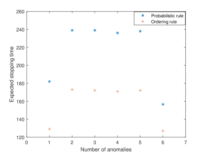
(a) Homogeneous setup

(b) Heterogeneous setup

Figure 1: Expected time for stopping that corresponds to each sampling rule versus the number of anomalous sources.

For each value of the true, but unknown, number of anomalous sources $m\in\{l,\ldots,u\}$, we compute the expected time until stopping for each one of the two sampling rules, when the true subset of anomalous sources is of the form $\{1,\ldots,m\}$. In all cases, the Monte Carlo error that corresponds to each estimated expected value is negligible (approximately $10^{-2}$).

In Figures 1a and 1b, we plot the resulting expected times until stopping against $m\in\{l,\ldots,u\}$ in the homogeneous and non-homogeneous setup, respectively. We observe that, in both setups and for both sampling rules, the induced expected time until stopping is much smaller when the number of anomalous sources is equal to either $\ell$ or $u$ than when it is between $\ell$ and $u$. Moreover, we observe that, in all cases, the ordering sampling rule leads to much smaller expected time until stopping than the corresponding probabilistic sampling rule.

7 Conclusion

In this paper, we consider the problem of sequential identification of anomalies under a general sampling constraint, where it is not necessary to sample only one source per time instant, and we allow for arbitrary bounds on the number of anomalous data sources. We introduce an ordering sampling rule, whose main feature is that the sources that are selected for sampling at each time are not determined solely based on the currently estimated subset of anomalous sources, but also on the ordering of the LLR statistics. We show that, with an appropriate design, such a sampling rule, combined with appropriate stopping and decision rules, leads to asymptotic optimality. That is, it minimizes the expected time for stopping, under any possible anomalous subset, to a first-order asymptotic approximation as the error rates go to 0. A novel proof technique is developed for this result that covers, for the first time, the case of multiple sampled sources per time instant, and the case that the number of anomalies is not necessarily known a priori to be equal to 1.

Following the same approach as in [16], the asymptotic optimality theory of the present paper can be shown to remain valid in the case of error metrics that are bounded up to a multiplicative constant by the corresponding classical familywise error rates. These include the false discovery rate (FDR) and the false non-discovery rate (FNR) [4], as well as the respective generalized FDR, FNR [2]. However, this direct extension is not possible under other kinds of error control, such as when it is required to control generalized familywise error rates, or the generalized misclassification error rate. This kind of error control has been considered in the absence of sampling constraints in [30], and with probabilistic sampling rules in [34]. Thus, extending the asymptotic optimality theory of the present under such generalized error metrics is a potential generalization of the present work.

Other relatively straightforward extensions of the present work include the incorporation of more general and multiple hypotheses per source, non-uniform sampling cost per observation in different sources, as in [14], a hierarchical structure of the sources, as in [12]. Finally, other interesting directions for future research include the proof of higher-order asymptotic optimality properties, as in [24], and the application of ordering sampling rules to non-sequential testing problems with adaptive design, as in [21].

Appendix A Definition of $x(A)$ and $y(A)$

For the definition of $x(A)$ and $y(A)$ we set

$$\theta_{A} :=I^{*}_{A}/J^{*}_{A}$$

$$z_{A} :=\theta_{A}/(r-1),\quad \mbox{if }\,r>1$$

$$w_{A} :=(1/\theta_{A})/(1/r-1),\quad \mbox{if }\,r<1.$$

A. We start with the case where the number of anomalies is known, i.e. $1\leq\ell=u\leq M-1$, and we distinguish two cases:

• If $\hat{K}(A)\leq\theta_{A}\,\check{K}(A)$, then

  $$x(A) :=(K/\hat{K}(A))\wedge 1,$$

  $$y(A) :=\left((K-\hat{K}(A))^{+}/\check{K}(A)\right)\wedge 1.$$

• If $\hat{K}(A)>\theta_{A}\,\check{K}(A)$, then

  $$x(A) :=\left((K-\check{K}(A))^{+}/\hat{K}(A)\right)\wedge 1,$$

  $$y(A) :=(K/\check{K}(A))\wedge 1.$$

B. We continue with the case where the number of anomalies is unknown, i.e., $0\leq\ell<u\leq M$, and we distinguish the following three cases.

• If $\ell<|A|<u$, then

  $$x(A) :=\frac{K}{\hat{K}(A)+(\theta_{A}/r)\check{K}(A)}\wedge(r/\theta_{A})\wedge 1,$$

  $$y(A) :=(\theta_{A}/r)\,x(A).$$

  
  

• If $|A|=\ell$, then we distinguish three subcases:
  

  • If $\ell=0$ or $r\leq 1$, then

    $$x(A) :=0,$$

    $$y(A) :=(K/\check{K}(A))\wedge 1.$$

  • If $\ell>0$, $r>1$, $z_{A}<1$, and $K>\hat{K}(A)+z_{A}\,\check{K}(A)$, then

    $$x(A) :=1,$$

    $$y(A) :=\bigl{(}(K-\hat{K}(A))/\check{K}(A)\bigr{)}\wedge 1.$$

  • If $\ell>0$, $r>1$, and either $z_{A}\geq 1$ or $K\leq\hat{K}(A)+z_{A}\,\check{K}(A)$, then

    $$x(A) :=\frac{K}{\hat{K}(A)+z_{A}\,\check{K}(A)}\wedge(1/z_{A})\wedge 1,$$

    $$y(A) :=\frac{K}{\check{K}(A)+(1/z_{A})\,\hat{K}(A)}\wedge z_{A}\wedge 1.$$

• If $|A|=u$, then we distinguish three subcases.
  

  • If $u=M$ or $r\geq 1$, then

    $$x(A) :=(K/\hat{K}(A))\wedge 1,$$

    $$y(A) :=0.$$

  • If $u<M$, $r<1$, $w_{A}<1$, and $K>\check{K}(A)+w_{A}\hat{K}(A)$, then

    $$x(A) :=\bigl{(}(K-\check{K}(A))/\hat{K}(A)\bigr{)}\wedge 1,$$

    $$y(A) :=1.$$

  • If $u<M$, $r<1$, and either $w_{A}\geq 1$ or $K\leq\check{K}(A)+w_{A}\hat{K}(A)$, then

    $$x(A) :=\frac{K}{\hat{K}(A)+(1/w_{A})\check{K}(A)}\wedge w_{A}\wedge 1,$$

    $$\quad y(A) :=\frac{K}{\check{K}(A)+w_{A}\hat{K}(A)}\wedge(1/w_{A})\wedge 1.$$

Appendix B

In Appendix B, we state and prove auxiliary lemmas that are used to establish the main results of the paper. Throughout this Appendix, we fix an arbitrary sampling rule $R$ and a set $A\in\mathcal{P}_{\ell,u}$. For any $i\in[M]$, we set

$$\begin{split}\bar{\Lambda}^{R}_{i}(n)&:=\bar{\Lambda}^{R}_{i}(n-1)+\Bigl{(}g_{i}(X_{i}(n))-\mathsf{E}_{A}[g_{i}(X_{i}(n))]\Bigr{)}\,R_{i}(n),\quad n\in\mathbb{N},\\ \bar{\Lambda}^{R}_{i}(0)&:=0,\end{split}$$ (97)

and we can easily verify that $\{\bar{\Lambda}^{R}_{i}(n):n\in\mathbb{N}_{0}\}$ is a zero-mean $\{\mathcal{F}^{R}(n):n\in\mathbb{N}_{0}\}$-martingale under $\mathsf{P}_{A}$. Comparing with (14), we observe that, for all $n\in\mathbb{N}_{0}$,

$$\bar{\Lambda}^{R}_{i}(n) =\begin{cases}\Lambda^{R}_{i}(n)-I_{i}\,N^{R}_{i}(n),\quad i\in A,\\ \Lambda^{R}_{i}(n)+J_{i}\,N^{R}_{i}(n),\quad i\notin A.\end{cases}$$ (98)

For each $i\in[M]$ and $n,m\in\mathbb{N}_{0}$, we denote by $\Lambda^{R}_{i}(n:m)$ the LLR statistic based on the measurements from source $i$ during $[m+1,n+m]$, i.e.,

$$\Lambda^{R}_{i}(n:m):=\Lambda^{R}_{i}(n+m)-\Lambda^{R}_{i}(m),$$ (99)

and we also set

$$\bar{\Lambda}^{R}_{i}(n:m):=\frac{1}{n}\Lambda^{R}_{i}(n:m).$$

We also recall the definition of $\pi^{R}_{i}(n:m)$ in (12) as the proportion of times source $i$ is sampled during $[m+1,m+n]$.

Moreover, given a family of events $\{E(n,\tau):n\in\mathbb{N}_{0},\tau\in\mathcal{T}_{A}\}$, we say that the conditional probability of $E(n,\tau)$ given $\mathcal{F}^{R}(\tau)$ is

• uniformly exponentially decaying if there are $C,\,c>0$, independent of $\tau\in\mathcal{T}_{A}$ and $n\in\mathbb{N}_{0}$, so that

  $$\mathsf{P}_{A}\left(E(n,\tau)\,|\,\mathcal{F}^{R}(\tau)\right)\leq C\,e^{-cn},\quad\mbox{ a.s.}$$ (100)

• uniformly $q$-polynomially decaying, for some $q>0$, if there is $C>0$, independent of $\tau\in\mathcal{T}_{A}$ and $n\in\mathbb{N}_{0}$, so that

  $$\mathsf{P}_{A}\left(E(n,\tau)\,|\,\mathcal{F}^{R}(\tau)\right)\leq C\,n^{-q},\quad\mbox{ a.s.}$$ (101)

Lemma B.1.

Let $\zeta\in(0,1]$, $\epsilon>0$. Then,

$$\mathsf{P}_{A} \left(\exists\,m\geq\zeta n:\,\bar{\Lambda}^{R}_{i}(m:\tau)<-\epsilon\,m\,|\,\mathcal{F}^{R}(\tau)\right),\quad\forall\;i\in A,$$ (102)

$$\mathsf{P}_{A} \left(\exists\,m\geq\zeta n:\,\bar{\Lambda}^{R}_{i}(m:\tau)>\epsilon\,m\,|\,\mathcal{F}^{R}(\tau)\right),\quad\forall\;i\notin A$$

are uniformly exponentially decaying.

Remark B.1.

This is a generalization of [35, Lemma A.1], which corresponds to the special case that $\tau=0$.

Proof.

We only prove the inequality for $i\in A$, as the proof for $i\notin A$ is similar. Thus, we fix $i\in A$. It suffices to show that there is a constant $c>0$ so that, for every $\tau\in\mathcal{T}_{A}$ and $m\in\mathbb{N}$,

$$\mathsf{P}_{A}\left(\bar{\Lambda}^{R}_{i}(m:\tau)<-\epsilon\,m\,|\,\mathcal{F}^{R}(\tau)\right)\leq e^{-cm},\quad\text{a.s.}$$ (103)

or, equivalently,

$$\mathsf{P}_{A}\left(\bar{\Lambda}^{R}_{i}(m:\tau)<-\epsilon\,m,\,B\right)\leq e^{-c\,m}\,\mathsf{P}_{A}(B),\quad\forall\;B\in\mathcal{F}^{R}(\tau).$$

Then, inequality (102) will follow by the law of total probability over all $m\geq\zeta n$, and (103).

In order to show (103), we fix $m\in\mathbb{N}$, $\tau\in\mathcal{T}_{A}$, $B\in\mathcal{F}^{R}(\tau)$. Since $\mathsf{P}_{A}(\tau<\infty)=1$, by the law of total probability we have

$$\mathsf{P}_{A}\left(\bar{\Lambda}^{R}_{i}(m:\tau)<-\epsilon\,m,B\right)=\sum_{u=0}^{\infty}\mathsf{P}_{A}\left(\bar{\Lambda}^{R}_{i}(m:u)<-\epsilon\,m,B,\tau=u\right).$$

Since $B\cap\{\tau=u\}\in\mathcal{F}^{R}(u)$ for every $u\in\mathbb{N}_{0}$, working similarly to [35, Lemma A.1] we can show that there is a constant $c>0$ so that, for every $u\in\mathbb{N}_{0}$,

$$\mathsf{P}_{A}\left(\bar{\Lambda}^{R}_{i}(m:u)<-\epsilon\,m,B,\tau=u\right)\leq e^{-c\,m}\,\mathsf{P}_{A}(\tau=u,B).$$

Summing over all $u\in\mathbb{N}_{0}$, we obtain (103). ∎

Lemma B.2.

Let $\zeta\in(0,1]$, $\epsilon>0$. Suppose condition (4) holds for some $\mathfrak{p}\geq 2$. Then,

$$\mathsf{P}_{A} \left(\exists\,m\in[\zeta n,n]:\,\bar{\Lambda}^{R}_{i}(m:\tau)\geq\epsilon\,m\,|\,\mathcal{F}^{R}(\tau)\right)\quad\forall\;i\in A,$$

$$\mathsf{P}_{A} \left(\exists\,m\in[\zeta n,n]:\,\bar{\Lambda}^{R}_{i}(m:\tau)\leq-\epsilon\,m\,|\,\mathcal{F}^{R}(\tau)\right)\quad\forall\;i\notin A,$$

are uniformly $\mathfrak{p}/2$-polynomially decaying.

Proof.

We prove the lemma for $i\in A$, as the proof for $i\notin A$ is similar. We fix $i\in A$, $B\in\mathcal{F}^{R}(\tau)$, and $n\in\mathbb{N}$. Since $\mathsf{P}_{A}(\tau<\infty)=1$, by the law of total probability we have

$$\mathsf{P}_{A} \left(\exists\,m\in[\zeta n,n]:\,\bar{\Lambda}^{R}_{i}(m:\tau)\geq\epsilon\,m,B\right)$$ (104)

$$= \sum_{u=0}^{\infty}\mathsf{P}_{A}\left(\exists\,m\in[\zeta n,n]:\bar{\Lambda}^{R}_{i}(m:u)\geq\epsilon\,m,B,\tau=u\right).$$

Since $m\geq\zeta n$, it holds

$$\mathsf{P}_{A}\left(\exists\,m\in[\zeta n,n]:\,\bar{\Lambda}^{R}_{i}(m:u)\geq\epsilon\,m,B,\;\tau=u\right)$$

$$\leq\mathsf{P}_{A}\left(\exists\,m\in[\zeta n,n]:\,\bar{\Lambda}^{R}_{i}(m:u)\geq\epsilon\,\zeta\,n,B,\;\tau=u\right)$$

$$\leq\mathsf{P}_{A}\left(\max_{m\in[0,n]}\big{|}\bar{\Lambda}^{R}_{i}(m:u)\big{|}^{\mathfrak{p}}\geq(\epsilon\,\zeta\,n)^{\mathfrak{p}},B,\;\tau=u\right).$$

For each $u\in\mathbb{N}_{0}$, $\{\bar{\Lambda}^{R}_{i}(m:u)\,:\,m\in\mathbb{N}_{0}\}$ is a $\{\mathcal{F}^{R}(m+u)\,:\,m\in\mathbb{N}_{0}\}$-martingale. Thus, by Doob’s submartingale inequality we have

$$\mathsf{P}_{A}\left(\max_{m\in[0,n]}|\bar{\Lambda}^{R}_{i}(m:u)|^{\mathfrak{p}}\geq\epsilon^{\mathfrak{p}}(\zeta\,n)^{\mathfrak{p}},B,\tau=u\right)\leq\frac{\mathsf{E}_{A}\left[|\bar{\Lambda}^{R}_{i}(n:u)|^{\mathfrak{p}};B,\tau=u\right]}{(\zeta\epsilon)^{\mathfrak{p}}\,n^{\mathfrak{p}}},$$

and by Rosenthal’s inequality [15, Theorem 2.12] there is a $C_{0}>0$ such that

$$\mathsf{E}_{A}\left[|\bar{\Lambda}^{R}_{i}(n:u)|^{\mathfrak{p}};\,B,\tau=u\right]\leq C_{0}\,n^{\mathfrak{p}/2}\,\mathsf{P}_{A}(B,\tau=u).$$

Combining the previous inequalities, we conclude that

$$\mathsf{P}_{A}\left(\exists\,m\in[\zeta n,n]:\,\bar{\Lambda}^{R}_{i}(m:u)\geq\epsilon m,B,\;\tau=u\right)\leq C\,n^{-\mathfrak{p}/2}\,\mathsf{P}_{A}(B,\tau=u),$$

where $C:=C_{0}/(\zeta\epsilon)^{\mathfrak{p}}$. Then, summing over $u\in\mathbb{N}_{0}$ completes the proof. ∎

For the following lemma, we need to introduce the quantity

$$q_{A}:=\max\bigg{\{}\max\limits_{i\in A}I_{i}/I^{*}_{A},\,\max\limits_{i\notin A}J_{i}/J^{*}_{A}\bigg{\}}.$$ (105)

Lemma B.3.

Let $\zeta,\,\rho,\,\lambda\in(0,1]$.

• For all $i\in A$, $j\notin A$,

  $$\mathsf{P}_{A}\left(\exists\,m\geq\zeta n:\,\Lambda^{R}_{i}(m:\tau)<0,\,\pi^{R}_{i}(m:\tau)>\rho\,|\,\mathcal{F}^{R}(\tau)\right)$$

  $$\mathsf{P}_{A}\left(\exists\,m\geq\zeta n:\,\Lambda^{R}_{j}(m:\tau)>0,\,\pi^{R}_{j}(m:\tau)>\rho\,|\,\mathcal{F}^{R}(\tau)\right)$$

  $$\mathsf{P}_{A}\left(\exists\,m\geq\zeta n:\,\Lambda^{R}_{j}(m:\tau)>\Lambda^{R}_{i}(m:\tau),\,\pi^{R}_{i}(m:\tau)>\rho\,|\,\mathcal{F}^{R}(\tau)\right)$$

  $$\mathsf{P}_{A}\left(\exists\,m\geq\zeta\,n:\,\Lambda^{R}_{j}(m:\tau)>\Lambda^{R}_{i}(m:\tau),\,\pi^{R}_{j}(m:\tau)>\rho\,|\,\mathcal{F}^{R}(\tau)\right)$$

  are uniformly exponentially decaying.
  

• If $\lambda/\rho>q_{A}$ and condition (4) holds for some $\mathfrak{p}\geq 2$, then, for all $i,j\in A$,

  $$\mathsf{P}_{A} \left(\exists\,m\geq\zeta n:\,\Lambda^{R}_{i}(m:\tau){>}\Lambda^{R}_{j}(m:\tau),\,\pi^{R}_{i}(m:\tau){<}\rho,\,\pi^{R}_{j}(m:\tau){>}\lambda\,|\,\mathcal{F}^{R}(\tau)\right)$$ (106)

  is uniformly $\mathfrak{p}/2$-polynomially decaying.
  

• If $\lambda/\rho<1/q_{A}$ and condition (4) holds for some $\mathfrak{p}\geq 2$, then, for all $i,j\notin A$,

  $$\mathsf{P}_{A} \left(\exists\,m\geq\zeta\,n:\,\Lambda^{R}_{i}(m:\tau)>\Lambda^{R}_{j}(m:\tau),\,\pi^{R}_{i}(m:\tau)>\rho,\,\pi^{R}_{j}(m:\tau)<\lambda\,|\,\mathcal{F}^{R}(\tau)\right)$$

  is uniformly $\mathfrak{p}/2$-polynomially decaying.

Proof.

(i) We only prove the claim for the first and the third conditional probability, as the proofs for the second and the fourth, respectively, are similar. By decomposition (98) we obtain

$$\mathsf{P}_{A}\left(\exists\,m\geq\zeta n:\,\Lambda^{R}_{i}(m:\tau)<0,\,\pi^{R}_{i}(m:\tau)>\rho\,|\,\mathcal{F}^{R}(\tau)\right)$$

$$=\mathsf{P}_{A}(\exists\,m\geq\zeta n:\,\bar{\Lambda}^{R}_{i}(m:\tau)<-I_{i}\,\pi^{R}_{i}(m:\tau)\,m,\,\pi^{R}_{i}(m:\tau)>\rho\,|\,\mathcal{F}^{R}(\tau))$$

$$\leq\mathsf{P}_{A}\left(\exists\,m\geq\zeta\,n:\,\bar{\Lambda}^{R}_{i}(m:\tau)<-I_{i}\,\rho\,m\,|\,\mathcal{F}^{R}(\tau)\right).$$

Similarly,

$$\mathsf{P}_{A}\left(\exists\,m\geq\zeta\,n:\,\Lambda^{R}_{j}(m:\tau)>\Lambda^{R}_{i}(m:\tau),\,\pi^{R}_{i}(m:\tau)>\rho\,|\,\mathcal{F}^{R}(\tau)\right)$$

$$=\mathsf{P}_{A}\bigg{(}\exists\,m\geq\zeta\,n:\,\bar{\Lambda}^{R}_{j}(m:\tau)-\bar{\Lambda}^{R}_{i}(m:\tau)>(I_{i}\pi^{R}_{i}(m:\tau)+J_{j}\pi^{R}_{j}(m:\tau))\,m,$$

$$\qquad\qquad\qquad\qquad\pi^{R}_{i}(m:\tau)>\rho\,|\,\mathcal{F}^{R}(\tau)\bigg{)}$$

$$\leq\mathsf{P}_{A}\left(\exists\,m\geq\zeta\,n:\,\bar{\Lambda}^{R}_{j}(m:\tau)-\bar{\Lambda}^{R}_{i}(m:\tau)>I_{i}\,\rho\,m\,|\,\mathcal{F}^{R}(\tau)\right)$$

$$\leq\mathsf{P}_{A}\left(\exists\,m\geq\zeta\,n:\,\bar{\Lambda}^{R}_{j}(m:\tau)>I_{i}\,(\rho/2)\,m\,|\,\mathcal{F}^{R}(\tau)\right)$$

$$\quad+\mathsf{P}_{A}\left(\exists\,m\geq\zeta\,n:\,-\bar{\Lambda}^{R}_{i}(m:\tau)>I_{i}\,(\rho/2)\,m\,|\,\mathcal{F}^{R}(\tau)\right).$$

In both cases, each term in the upper bound is uniformly exponentially decaying by Lemma B.1, which proves the claim.

For (ii) (similarly for (iii)), by decomposition (98), the conditional probability in (106) can be expressed as

$$\mathsf{P}_{A} \Big{(}\exists\,m\geq\zeta\,n:\,\bar{\Lambda}^{R}_{i}(m:\tau)-\bar{\Lambda}^{R}_{j}(m:\tau)>(I_{j}\,\pi^{R}_{j}(m:\tau)-I_{i}\,\pi^{R}_{i}(m:\tau)\big{)}m$$

$$\qquad\qquad\qquad\quad\pi^{R}_{i}(m:\tau)<\rho,\,\pi^{R}_{j}(m:\tau)>\lambda\,|\,\mathcal{F}^{R}(\tau)\Big{)}$$

and is bounded by

$$\mathsf{P}_{A}(\exists\,m\geq\zeta\,n:\,\bar{\Lambda}^{R}_{i}(m:\tau)-\bar{\Lambda}^{R}_{j}(m:\tau)>(I_{j}\lambda-I_{i}\rho)m\,|\,\mathcal{F}^{R}(\tau))$$

$$\leq\mathsf{P}_{A}(\exists\,m\geq\zeta\,n:\,\bar{\Lambda}^{R}_{i}(m:\tau)>(I_{j}\lambda-I_{i}\rho)\,m/2\,|\,\mathcal{F}^{R}(\tau))$$

$$\qquad+\mathsf{P}_{A}(\exists\,m\geq\zeta\,n:\,-\bar{\Lambda}^{R}_{j}(m:\tau)>(I_{j}\,\lambda-I_{i}\,\rho)\,m/2\,|\,\mathcal{F}^{R}(\tau)),$$

where $I_{j}\lambda-I_{i}\rho>0$ because $\lambda/\rho>q_{A}$. The first term on the right hand side is uniformly $\mathfrak{p}/2$-polynomially decaying by Lemma B.2, and the second term is uniformly exponentially decaying by Lemma B.1, which proves the claim. ∎

Last, we provide a lemma about the maximum draw-down of the LLRs.

Lemma B.4.

Let $\tau\in\mathcal{T}_{A}$ and $x>0$, then

$$\mathsf{P}_{A}\left(\Lambda^{R}_{i}(\tau)-\inf_{n\geq\tau}\Lambda^{R}_{i}(n)>x\right) \leq e^{-x},\quad\forall\,i\in A,$$ (107)

$$\mathsf{P}_{A}\left(\sup_{n\geq\tau}\Lambda^{R}_{i}(n)-\Lambda^{R}_{i}(\tau)>x\right) \leq e^{-x},\quad\forall\,i\notin A.$$

Consequently, the random variables $\Lambda^{R}_{i}(\tau)-\inf_{n\geq\tau}\Lambda^{R}_{i}(n)$ and $\;\sup_{n\geq\tau}\Lambda^{R}_{i}(n)-\Lambda^{R}_{i}(\tau)$ have each moment bounded by a constant that does not depend on $\tau\in\mathcal{T}_{A}$.

Proof.

We only prove the claim for $i\in A$, as the proof for $i\notin A$ is similar. We note that

$$\Lambda^{R}_{i}(\tau)-\inf_{n\geq\tau}\Lambda^{R}_{i}(n)=-\inf_{n\in\mathbb{N}}\Lambda^{R}_{i}(n:\tau)=\sup_{n\in\mathbb{N}}\left\{-\Lambda^{R}_{i}(n:\tau)\right\}.$$ (108)

For any $x>0$,

$$\mathsf{P}_{A}\left(\sup_{n\in\mathbb{N}}\{-\Lambda^{R}_{i}(n:\tau)\}>x\right)=\mathsf{P}_{A}\left(\sup_{n\in\mathbb{N}}\left\{\exp(-\Lambda^{R}_{i}(n:\tau))\right\}>e^{x}\right).$$ (109)

Since $\mathsf{P}_{A}(\tau<\infty)=1$, by the law of total probability we have

$$\mathsf{P}_{A}\left(\sup_{n\in\mathbb{N}}\{-\Lambda^{R}_{i}(n:\tau)\}>x\right)=\sum_{m=0}^{\infty}\mathsf{P}_{A}\left(\sup_{n\in\mathbb{N}}\left\{\exp(-\Lambda^{R}_{i}(n:m))\right\}>e^{x},\tau=m\right).$$ (110)

We note that, for any $n,\,m\in\mathbb{N}_{0}$, $X_{i}(n+1+m)$ is independent of $\mathcal{F}^{R}(n+m)$, and it has the same distribution as $X_{i}(1)$ [11, Theorem 4.1.3]. Since $R_{i}(n+1+m)\in\{0,1\}$ and $X_{i}(n+1+m)$ is $\mathcal{F}^{R}(n+m)$-measurable, it holds

$$\mathsf{E}_{A} \left[\exp\{-g_{i}(X_{i}(n+1+m))\,R_{i}(n+1+m)\}\,|\,\mathcal{F}^{R}(n+m)\right]$$ (111)

$$=\mathsf{E}_{A}\left[\exp\{-g_{i}(X_{i}(1))\}\right]^{R_{i}(n+1+m)}=1.$$

This implies that, for fixed $m\in\mathbb{N}_{0}$, $\{\exp\{-\Lambda^{R}_{i}(n:m)\}\,:\,n\in\mathbb{N}_{0}\}$ is a martingale with respect to $\{\mathcal{F}^{R}(n+m)\,:\,n\in\mathbb{N}_{0}\}$. Thus, by Ville’s supermartingale inequality we have, for any $m\in\mathbb{N}_{0}$,

$$\mathsf{P}_{A}\left(\sup_{n\in\mathbb{N}}\left(\exp\{-\Lambda^{R}_{i}(n:m)\}\right)>e^{x},\,\tau=m\right)\leq e^{-x}\,\mathsf{P}_{A}(\tau=m).$$

Then, summing over all $m\in\mathbb{N}_{0}$ completes the proof. ∎

Appendix C

In Appendix C, we prove the consistency criterion in Theorem 3.2 applying Lemma B.3 with $\tau=0$.

Proof of Theorem 3.2.

By the definition of $\Delta^{R}$ and the definition of $\sigma_{A}^{R}$, we have the following inequalities:

if $\ell=u$, then

$$\mathsf{P}_{A}(\sigma_{A}^{R}>n)\leq\sum\limits_{i\in A,\,j\notin A}\mathsf{P}_{A}\left(\exists\,m\geq n:\,\Lambda^{R}_{j}(m)\geq{\Lambda}^{R}_{i}(m)\right),$$ (112)

if $\ell<|A|<u$, then

$$\begin{split}\mathsf{P}_{A}(\sigma_{A}^{R}>n)\leq&\sum\limits_{i\in A}\mathsf{P}_{A}\left(\exists\,m\geq n:\,\Lambda^{R}_{i}(m)<0\right)\\ &+\sum\limits_{j\notin A}\mathsf{P}_{A}\left(\exists\,m\geq n:\,\Lambda^{R}_{j}(m)\geq 0\right),\end{split}$$ (113)

if $|A|=\ell$, then

$$\begin{split}\mathsf{P}_{A}(\sigma_{A}^{R}>n)\leq&\sum\limits_{j\notin A}\mathsf{P}_{A}\left(\exists\,m\geq n:\,\Lambda^{R}_{j}(m)\geq 0\right)\\ &+\sum\limits_{i\in A,\,j\notin A}\mathsf{P}_{A}(\exists\,m\geq n:\,\Lambda^{R}_{j}(m)\geq{\Lambda}^{R}_{i}(m)),\end{split}$$ (114)

if $|A|=u$, then

$$\begin{split}\mathsf{P}_{A}(\sigma_{A}^{R}>n)\leq&\sum\limits_{i\in A}\mathsf{P}_{A}\left(\exists\,m\geq n:\,\Lambda^{R}_{i}(m)<0\right)\\ &+\sum\limits_{i\in A,\,j\notin A}\mathsf{P}_{A}\left(\exists\,m\geq n:\,\Lambda^{R}_{j}(m)\geq{\Lambda}^{R}_{i}(m)\right).\end{split}$$ (115)

By the above inequalities and Proposition 3.2, we conclude that it suffices to show the following:

• If $x(A)>0$, then, for all $i\in A$ and $j\notin A$,

  $$\sum_{n=1}^{\infty}\mathsf{P}_{A}\left(\exists\,m\geq n:\,\Lambda^{R}_{j}(m)\geq{\Lambda}^{R}_{i}(m)\right)\ <\infty,$$

  $$\text{and}\quad\sum_{n=1}^{\infty}\mathsf{P}_{A}\left(\exists\,m\geq n:\,\Lambda^{R}_{i}(m)<0\right)\, <\,\infty.$$

• If $y(A)>0$, then, for all $i\in A$ and $j\notin A$,

  $$\sum_{n=1}^{\infty}\mathsf{P}_{A}\left(\exists\,m\geq n:\,\Lambda^{R}_{j}(m)\geq{\Lambda}^{R}_{i}(m)\right) <\,\infty,$$

  $$\text{and}\quad\sum_{n=1}^{\infty}\mathsf{P}_{A}\left(\exists\,m\geq n:\,\Lambda^{R}_{j}(m)\geq 0\right) <\,\infty.$$

We only prove the case $x(A)>0$, as the proof for $y(A)>0$ is similar. To this end, we fix $i\in A$, $j\notin A$. For every $\rho>0$, we have

$$\mathsf{P}_{A}\left(\exists\,m\geq n:\,\Lambda^{R}_{j}(m)\geq{\Lambda}^{R}_{i}(m)\right) =\mathsf{P}_{A}\left(\exists\,m\geq n:\,\Lambda_{j}(m)\geq{\Lambda}_{i}(m),\,\pi^{R}_{i}(m)\geq\rho\right)$$ (116)

$$+\mathsf{P}_{A}\left(\exists\,m\geq n:\,\pi^{R}_{i}(m)<\rho\right),$$

and

$$\mathsf{P}_{A}\left(\exists\,m\geq n:\,\Lambda^{R}_{i}(m)<0\right) =\mathsf{P}_{A}\left(\exists\,m\geq n:\,\Lambda^{R}_{i}(m)<0,\,\pi^{R}_{i}(m)\geq\rho\right)$$ (117)

$$+\mathsf{P}_{A}\left(\exists\,m\geq n:\,\pi^{R}_{i}(m)<\rho\right).$$

In (116) (resp. (117)), the first term on the right hand side is summable by (iii) ( resp. (i)) of Lemma B.3. For the second term we observe that

$$\sum_{n=1}^{\infty}\mathsf{P}_{A}(\exists\,m\geq n:\,\pi^{R}_{i}(m)<\rho)\leq\sum_{n=1}^{\infty}\sum_{m=n}^{\infty}\mathsf{P}_{A}(\pi^{R}_{i}(m)<\rho)=\sum_{n=1}^{\infty}n\mathsf{P}_{A}(\pi^{R}_{i}(n)<\rho).$$

Thus, it suffices to select $\rho>0$ so that the sequence $\{n\,\mathsf{P}_{A}(\pi^{R}_{i}(n)<\rho)\,:\,n\in\mathbb{N}\}$ is summable. This is indeed possible, by the assumption of the theorem. ∎

Appendix D

In this Appendix, we prove Theorem 4.1. Throughout this Appendix we fix $A\in\mathcal{P}_{\ell,u}$, and an arbitrary ordering sampling rule $R$ that satisfies the conditions of Theorem 4.1.

For any $n\in\mathbb{N}$ and non-empty set $V\subseteq[M]$, we introduce the event on which the statistics in $A\setminus V$ are positive and greater than those in $V$, and the statistics in $A^{c}\setminus V$ are negative and smaller than those in $V$, i.e.,

$$E_{A,V}(n):=\bigcap_{i\in A\setminus V}\bigcap_{j\in V}\bigcap_{z\in A^{c}\setminus V}\{\Lambda^{R}_{i}(n)\geq\max\{0,\Lambda^{R}_{j}(n)\}\geq\min\{0,\Lambda^{R}_{j}(n)\}\geq\Lambda^{R}_{z}(n)\}.$$

The proof of Theorem 4.1 relies on two results regarding this event, which are presented in Lemmas D.1 and D.2.

According to the first one, the event $E_{A,V}(n)$ has high probability if at time $n$ there have been collected relatively few samples from sources in $V$ and relatively many samples from sources not in $V$. To be precise, for some $\rho,\,\zeta\in(0,1)$, that will be selected appropriately later, we introduce the event

$$\Gamma_{V}(n):=\left\{\Pi_{V}(n)<\rho\right\}\bigcap\left\{\Pi_{V^{c}}(n)>\zeta\right\},$$ (118)

where

$$\left\{\Pi_{V}(n)<\rho\right\}: =\{\pi^{R}_{i}(n)<\rho,\,\forall\,i\in V\},$$

$$\left\{\Pi_{V^{c}}(n)>\zeta\right\} :=\{\pi^{R}_{i}(n)>\zeta,\,\forall\,i\notin V\}.$$

Lemma D.1.

Let $V\subseteq[M]$ and $\rho,\,\zeta\in(0,1)$ such that $\zeta>q_{A}\,\rho$, where $q_{A}$ is defined in (105). Suppose condition (4) holds for some $\mathfrak{p}\geq 2$. Then,

$$\mathsf{P}_{A}\left(\bigcup_{m=\lceil n/2\rceil}^{n}\,E^{c}_{A,V}(m:\tau)\cap\Gamma_{V}(m:\tau)\,\Big{|}\,\mathcal{F}^{R}(\tau)\right)$$ (119)

is uniformly $\mathfrak{p}/2$-polynomially decaying.

Proof.

For $m\in[n/2,n]$, one of the following holds on the event $E^{c}_{A,V}(m:\tau)$:

• $\exists\;i\in A\setminus V$ and $j\in V\cap A$ such that $\Lambda_{i}(m:\tau)<\Lambda_{j}(m:\tau)$,
  

• $\exists\;i\in A\setminus V$ and $k\in V\setminus A$ such that $\Lambda_{i}(m:\tau)<\Lambda_{k}(m:\tau)$,
  

• $\exists\;i\in A\setminus V$ such that $\Lambda_{i}(m:\tau)<0$,
  

• $\exists\;j\in V\cap A$ and $z\in A^{c}\setminus V$ such that $\Lambda_{j}(m:\tau)<\Lambda_{z}(m:\tau)$,
  

• $\exists\;k\in V\setminus A$ and $z\in A^{c}\setminus V$ such that $\Lambda_{k}(m:\tau)<\Lambda_{z}(m:\tau)$,
  

• $\exists\;z\in A^{c}\setminus V$ such that $\Lambda_{z}(m:\tau)>0$.

As a result, by Boole’s inequality, it suffices to show that, for any $i\,\in\,A\setminus V$, $j\,\in\,V\cap A$, $k\,\in\,V\setminus A$, $z\,\in A^{c}\setminus V$,

$$\mathsf{P}_{A}\left(\exists\,m\in[n/2,n]:\,\Lambda^{R}_{i}(m:\tau)<\Lambda^{R}_{j}(m:\tau),\,\Gamma_{V}(m:\tau)\,\Big{|}\,\mathcal{F}^{R}(\tau)\right),$$ (120)

$$\mathsf{P}_{A}\left(\exists\,m\in[n/2,n]:\,\Lambda^{R}_{i}(m:\tau)<\Lambda^{R}_{k}(m:\tau),\,\Gamma_{V}(m:\tau)\,\Big{|}\,\mathcal{F}^{R}(\tau)\right)$$

$$\mathsf{P}_{A}\left(\exists\,m\in[n/2,n]:\,\Lambda^{R}_{i}(m:\tau)<0,\,\Pi_{V}(m:\tau)<\rho\Big{|}\,\mathcal{F}^{R}(\tau)\,\right)$$

$$\mathsf{P}_{A}\left(\exists\,m\in[n/2,n]:\,\Lambda^{R}_{j}(m:\tau)<\Lambda^{R}_{z}(m:\tau),\,\Gamma_{V}(m:\tau)\,\Big{|}\,\mathcal{F}^{R}(\tau)\right)$$

$$\mathsf{P}_{A}\left(\exists\,m\in[n/2,n]:\,\Lambda^{R}_{j}(m:\tau)<\Lambda^{R}_{z}(m:\tau),\,\Gamma_{V}(m:\tau)\,\Big{|}\,\mathcal{F}^{R}(\tau)\right),$$

$$\mathsf{P}_{A}\left(\exists\,m\in[n/2,n]:\,\Lambda^{R}_{z}(m:\tau)>0,\,\Pi_{V^{c}}(m:\tau)>\zeta\,\Big{|}\,\mathcal{F}^{R}(\tau)\right)$$

are uniformly $\mathfrak{p}/2$-polynomially decaying. This is indeed the case by Lemma B.3. ∎

According to the second result, if the sampling rule $R$ satisfies condition (36) of Theorem 4.1, then, for any $V\subseteq[M]$ that either intersects $A$ when $x(A)>0$ or $A^{c}$ when $y(A)>0$, it is unlikely to have only a few samples from $V$, if the event $E_{A,V}(m)$ occurs for every $m\in[n/2,n]$, especially when $n$ is large.

Lemma D.2.

Suppose the sampling rule $R$ satisfies (36) for some $\delta\in(0,1]$, and

$$\mbox{either}\;\;A\cap V\neq\emptyset\quad\mbox{when}\quad x(A)>0\;\;\ \qquad\mbox{or}\qquad A^{c}\cap V\neq\emptyset\quad\mbox{when}\;y(A)>0.$$ (121)

1. For any $m\in\mathbb{N}$, on the event $E_{A,V}(m)$, at least one source in $V$ is sampled at time $m+1$ with probability at least $\delta$.
   

2. If $\rho<\delta/(2|V|)$, then

   $$\mathsf{P}_{A}\left(\Pi_{V}(n:\tau)<\rho,\,\bigcap_{m=\lceil n/2\rceil}^{n}E_{A,V}(m:\tau)\,|\,\mathcal{F}^{R}(\tau)\right)$$ (122)

   is uniformly exponentially decaying.

Proof.

We prove the lemma when $x(A)>0$ and $A\cap V\neq\emptyset$. If this is not true, then by (121) it follows that $y(A)>0$ and $A^{c}\cap V\neq\emptyset$ and the proof is completely analogous.

(i) We fix $m\in\mathbb{N}$. It is clear that at least one source in $V$ is sampled at time $m+1$ when either $\hat{\mathcal{G}}(m)$ or $\check{\mathcal{G}}(m)$ intersects with $V$. Therefore, it suffices to show that at least one source in $V$ is sampled at time $m+1$, at least with probability $\delta>0$, also on the event

$$E_{A,V}(m)\cap\{V\subseteq\hat{\mathcal{G}}^{c}(m)\cap\check{\mathcal{G}}^{c}(m)\}.$$ (123)

By the definition of the ordering sampling rule, it suffices to show that on this event one of the following holds:

• $\hat{\mathcal{N}}(m)-|\hat{\mathcal{G}}(m)|>\delta$ and the source with the smallest LLR in $\Delta^{R}(m)\setminus\hat{\mathcal{G}}(m)\neq\emptyset$ is in $V$,
  

• $\check{\mathcal{N}}(m)-|\check{\mathcal{G}}(m)|>\delta$ and the source with the largest LLR in $(\Delta^{R}(m))^{c}\setminus\check{\mathcal{G}}(m)\neq\emptyset$ is in $V$.

In view of condition (36), it suffices to show that on the event (123) one of the following holds:

• $x(\Delta^{R}(m))>0$ and the source with the smallest LLR in $\Delta^{R}(m)\setminus\hat{\mathcal{G}}(m)\neq\emptyset$ is in $V$,
  

• $y(\Delta^{R}(m))>0$ and the source with the largest LLR in $(\Delta^{R}(m))^{c}\setminus\hat{\mathcal{G}}(m)\neq\emptyset$ is in $V$.

By Proposition 3.2(iii) and (iv), for every $D\in\mathcal{P}_{\ell,u}$,

$$x(D)=0\;\Rightarrow\;y(D)>0,\quad\mbox{ and }\quad y(D)=0\;\Rightarrow\;x(D)>0.$$

Thus, it suffices to show that, for every $D\in\mathcal{P}_{\ell,u}$ and $G,\,G^{\prime}\subseteq[M]$, on the event

$$E_{A,V}(m)\cap\{V\subseteq\hat{\mathcal{G}}^{c}(m)\cap\check{\mathcal{G}}^{c}(m)\}\cap\{\Delta^{R}(m)=D\}\cap\{\hat{\mathcal{G}}(m)=G\}\cap\{\check{\mathcal{G}}(m)=G^{\prime}\}$$ (124)

the following claims hold:

• If $D\setminus G\neq\emptyset$ and $y(D)=0$, then the source with the smallest LLR in $D\setminus G$ is in $V$,
  

• If $D^{c}\setminus G^{\prime}\neq\emptyset$ and $x(D)=0$, then the source with the largest LLR in $D^{c}\setminus G^{\prime}$ is in $V$,
  

• If $x(D)>0$ and $y(D)>0$, then either the source with the smallest LLR in $D\setminus G$ or the source with the largest LLR in $D^{c}\setminus G^{\prime}$ is in $V$.
  

In what follows, we assume that the event (124) is non-empty, otherwise there is nothing to prove. We note that this implies that at least one of the sets $D\setminus G$ and $D^{c}\setminus G^{\prime}$ is non-empty. Otherwise, we would have $D=G$, $D^{c}=G^{\prime}$ and $V=\emptyset$, which implies that the event (124) would be empty. We continue with the proof of each one of the claims (a)-(c) on the event (124).

Suppose $D\setminus G\neq\emptyset$ and $y(D)=0$. Then, by Proposition 3.2(iv) it holds $|D|=u$. In this case, by the form of the decision rule in Subsection 3.2 we have that $D$ consists of the sources with the $u$ largest LLR statistics at time $m$. By the definition of $E_{A,V}(m)$ it follows that at time $m$ the sources in $A\setminus V$ have positive LLRs, which are larger than those in $V$. Thus, $A\setminus V\subseteq D$. Also, since $|A|\leq u$, and $A\setminus V\neq\emptyset$, by assumption, we have $|A\setminus V|<u=|D|$. This proves that on the event (124) the source with the smallest LLR in $D\setminus G$ is in $V$.

Suppose $D^{c}\setminus G^{\prime}\neq\emptyset$ and $x(D)=0$. Then, by Proposition 3.2(iii) it holds $|D|=\ell\Leftrightarrow|D^{c}|=M-\ell$. By the form of the decision rule in Subsection 3.2 it follows that $D^{c}$ consists of the sources with the $M-\ell$ smallest LLR statistics at time $m$. By the definition of $E_{A,V}(m)$ we have that at time $m$ the sources in $A^{c}\setminus V$ have negative LLRs which are smaller than those in $V$. Thus, $A^{c}\setminus V\subseteq D^{c}$. In view of the fact $|A|\geq\ell\Leftrightarrow|A^{c}|\leq M-\ell$, which implies $|A^{c}\setminus V|\leq M-\ell$, we consider two subcases depending on whether the latter inequality is strict or it holds by equality.

• Suppose first that $|A^{c}\setminus V|=M-\ell$, in which case $A^{c}\setminus V=A^{c}$ and $|A^{c}|=M-\ell$. Then, the event (124) is equal to the empty set. To show this, we argue by contradiction. Indeed, if this is not the case, then by $A^{c}\subseteq D^{c}$ and $|A^{c}|=|D^{c}|=M-\ell$, we conclude that $A^{c}=D^{c}$, and consequently, $A=D$ and $x(D)=x(A)$. However, $x(A)$ is assumed to be positive and $x(D)$ to be equal to $0$, which is a contradiction.
  

• Suppose next that $|A^{c}\setminus V|<M-\ell$. Since $|A^{c}\setminus V|<M-\ell=|D^{c}|$, on the event (124) the source with the largest LLR in $D^{c}\setminus G^{\prime}$ is in $V$.
  

Let $x(D)>0$ and $y(D)>0$. If $|D|=u$, the result follows from (a), whereas if $|D|=\ell$ the result follows from (b). Thus, it suffices to consider the case where $\ell<|D|<u$. By the form of the decision rule in Subsection 3.2, $D$ consists of the sources with positive LLRs at time $m$. By the definition of $E_{A,V}(m)$ it follows that at time $m$ the sources in $A\setminus V$ have positive LLRs, which are larger than those in $V$, and the sources in $A^{c}\setminus V$ have negative LLRs, which are smaller than those in $V$. Thus, $A\setminus V\subseteq D$ and $A^{c}\setminus V\subseteq D^{c}$.

Since at least one of the previous two inclusions is strict (otherwise we would have $V=\emptyset$), we conclude that on the event (124) either the source with the smallest LLR in $D\setminus G$ or the source with the largest LLR in $D^{c}\setminus G^{\prime}$ is in $V$.

(ii) By (i) it follows that there is a sequence $\{Z_{0}(m)\,:\,m\in\mathbb{N}\}$ of iid Bernoulli random variables with parameter $\delta$ such that, for every $m\in\mathbb{N}$,

$$E_{A,V}(m)\subseteq\left\{\sum_{i\in V}R_{i}(m+1)\geq Z_{0}(m)\right\}.$$ (125)

Let $\tau\in\mathcal{T}_{A}$, $n\in\mathbb{N}$, and let $W_{V}(n/2;\tau)$ denote the total number of samples from the sources in $V$ during $[\tau+n/2,\tau+n]$, i.e.,

$$W_{V}(n/2;\tau):=\sum_{m=\lceil n/2\rceil}^{n}\sum_{i\in V}R_{i}(\tau+m).$$ (126)

Then, by (i) it follows that

$$\bigcap_{m=\lceil n/2\rceil}^{n}E_{A,V}(m:\tau)\subseteq\left\{W_{V}(n/2;\tau)\geq\sum_{m=\lceil n/2\rceil}^{n}Z_{0}(\tau+m)\right\}.$$ (127)

If $\rho<\delta/(2|V|)$, then there exists $\epsilon\in(0,\delta)$ such that $\rho<(\delta-\epsilon)/(2|V|)$. Consequently, on the event $\{\Pi_{V}(n:\tau)<\rho\}$ we have

$$W_{V}(n/2;\tau)\leq\sum_{i\in V}n\,\pi_{i}(n:\tau)\leq\rho\,|V|\,n\leq(\delta-\epsilon)\lceil n/2\rceil.$$

Combining the above, we obtain

$$\left\{\Pi_{V}(n:\tau)<\rho,\,\bigcap_{m=\lceil n/2\rceil}^{n}E_{A,V}(m:\tau)\right\}\subseteq\left\{(\delta-\epsilon)\lceil n/2\rceil\geq\sum_{m=\lceil n/2\rceil}^{n}Z_{0}(m+\tau)\right\}.$$

Consequently,

$$\mathsf{P}_{A} \left(\Pi_{V}(n:\tau)<\rho,\,\bigcap_{m=\lceil n/2\rceil}^{n}E_{A,V}(m:\tau)\Big{|}\mathcal{F}^{R}(\tau)\right)$$ (128)

$$\leq\mathsf{P}_{A}\left((\delta-\epsilon)\lceil n/2\rceil\geq\sum_{m=\lceil n/2\rceil}^{n}Z_{0}(m+\tau)\Big{|}\mathcal{F}^{R}(\tau)\right)$$

$$=\mathsf{P}_{A}\left((\delta-\epsilon)\lceil n/2\rceil\geq\sum_{m=\lceil n/2\rceil}^{n}Z_{0}(m)\right),$$

where the equality holds because $\tau$ is a stopping time, $\{Z_{0}(m)\,:\,m\in\mathbb{N}_{0}\}$ is an iid sequence, $\{Z_{0}(m+\tau)\,:\,m\in\mathbb{N}_{0}\}$ is independent of $\mathcal{F}^{R}(\tau)$, and has the same distribution as $\{Z_{0}(m)\,:\,m\in\mathbb{N}_{0}\}$ [11, Theorem 4.1.3]. The upper bound is independent of $\tau$, and by the Chernoff bound it follows that it is exponentially decaying, which completes the proof. ∎

Proof of Theorem 4.1.

In order to show (37) for every $i\in A$ when $x(A)>0$, and for every $i\notin A$ when $y(A)>0$, it suffices to show that, for each $V\subseteq[M]$ that satisfies (121), there exist constants $\rho\in(0,1)$ and $C>0$ such that, for all $n\in\mathbb{N}$ and $\tau\in\mathcal{T}_{A}$,

$$\mathsf{P}_{A}\left(\Pi_{V}(n:\tau)<\rho\,\Big{|}\,\mathcal{F}^{R}(\tau)\right)\leq C\,n^{-\mathfrak{p}/2},\quad\mbox{a.s.},$$

i.e., the left-hand term is uniformly $\mathfrak{p}/2$-polynomially decaying, as defined in (101). As a result, for $V$ with size $|V|=1$, we obtain Theorem 4.1.

In view of Lemma D.2(ii), it suffices to show that, for every $V\subseteq[M]$ that satisfies (121), there exists a $\rho\in(0,1)$ such that

$$\mathsf{P}_{A}\left(\Pi_{V}(n:\tau)<\rho,\,\bigcup_{m=\lceil n/2\rceil}^{n}E^{c}_{A,V}(m:\tau)\,\Big{|}\,\mathcal{F}^{R}(\tau)\right)$$ (129)

is uniformly $\mathfrak{p}/2$-polynomially decaying.

To this end, we observe that, for any $\rho\in(0,1)$ and $V\subseteq[M]$,

$$\{\Pi_{V}(n:\tau)<\rho\}\subseteq\bigcap_{m=\lceil n/2\rceil}^{n}\{\Pi_{V}(m:\tau)<2\rho\}.$$ (130)

Indeed, on the event $\{\Pi_{V}(n:\tau)<\rho\}$, we have $\pi^{R}_{i}(n:\tau)<\rho$ for all $i\in V$. Thus, for any $m\in[n/2,\,n]$ we obtain

$$(n/2)\,\pi^{R}_{i}(m:\tau)\leq m\,\pi^{R}_{i}(m:\tau) =\sum_{u=1+\tau}^{m+\tau}R_{i}(u)$$ (131)

$$\leq\sum_{u=1+\tau}^{n+\tau}R_{i}(u)=\pi^{R}_{i}(n:\tau)\,n<\rho\,n.$$

Therefore, by (130) it follows that the sequence in (129) is bounded by

$$\mathsf{P}_{A} \left(\bigcap_{m=\lceil n/2\rceil}^{n}\{\Pi_{V}(m:\tau)<2\rho\},\,\bigcup_{m=\lceil n/2\rceil}^{n}E^{c}_{A,V}(m:\tau)\,\Big{|}\,\mathcal{F}^{R}(\tau)\right)$$ (132)

$$\leq\mathsf{P}_{A}\left(\bigcup_{m=\lceil n/2\rceil}^{n}\{\Pi_{V}(m:\tau)<2\rho\}\cap E^{c}_{A,V}(m:\tau)\,\Big{|}\,\mathcal{F}^{R}(\tau)\right),$$

which is further bounded by the sum

$$\mathsf{P}_{A} \left(\bigcup_{m=\lceil n/2\rceil}^{n}\{\Pi_{V}(m:\tau)<2\rho,\,\Pi_{V^{c}}(m:\tau)>\zeta\}\cap E^{c}_{A,V}(m:\tau)\,\Big{|}\,\mathcal{F}^{R}(\tau)\right)$$ (133)

$$+\mathsf{P}_{A}\left(\bigcup_{m=\lceil n/2\rceil}^{n}\{\Pi_{V}(m:\tau)<2\rho\}\cap\{\Pi_{V^{c}}(m:\tau)>\zeta\}^{c}\,\Big{|}\,\mathcal{F}^{R}(\tau)\right),$$

for any choice of $\zeta\in(0,1)$. By Lemma D.1, the first term in (133) is uniformly $\mathfrak{p}/2$-polynomially decaying for any $\rho,\,\zeta>0$ such that $\zeta>q_{A}2\rho$.

However, in order to show that the second term in (133) is also uniformly $\mathfrak{p}/2$-polynomially decaying, $\zeta$ and $\rho$ must be selected depending on the size of $V$, i.e., $\rho_{v}$, $\zeta_{v}$ for each $v\in[M]$. Of course, for each $v\in[M]$, $\rho_{v}$, $\zeta_{v}$ must satisfy

$$\rho_{v}<\delta/(2v),\quad\mbox{ and }\quad\zeta_{v}>2\rho_{v}q_{A},$$ (134)

as the first condition guarantees that (122) is uniformly exponentially decaying by Lemma D.2(ii), and the second guarantees that the first term in (133) is uniformly $\mathfrak{p}/2$-polynomially decaying by Lemma D.1. We will show that, for each $v\in[M]$, if we select $\rho_{v}$ and $\zeta_{v}$ such that, in addition to (134),

$$\max\{4\rho_{v},\,2\zeta_{v}\}<\rho_{v+1},$$ (135)

where $\rho_{M+1}:=\infty$, then the second term in (133) is uniformly $\mathfrak{p}/2$-polynomially decaying for every $V\subseteq[M]$ with $|V|=v$ that satisfies (121). In order to show this, we will apply a backward induction argument, starting from $v=M$ down to $v=1$.

If $v=M$, then $V=[M]$ or, equivalently, $V^{c}=\emptyset$, and as a result, the second term in (133) is trivially equal to zero for any $\rho,\,\zeta\in(0,1)$. Thus, in order to guarantee that

$$\mathsf{P}_{A}\left(\Pi_{[M]}(n:\tau)<\rho_{M}\,|\,\mathcal{F}^{R}(\tau)\right)$$

is uniformly $\mathfrak{p}/2$-polynomially decaying, it suffices to select $\rho_{M},\,\zeta_{M}$ that satisfy (134).

Now, suppose that the claim holds for $v+1$, i.e., there exist $\rho_{v+1},\,\zeta_{v+1}\in(0,1)$ such that the second term in (133) is uniformly $\mathfrak{p}/2$-polynomially decaying for any $|V|=v+1$ that satisfies (121). We will show that the claim also holds for $v$. For this, we fix $\rho_{v}$, $\zeta_{v}$ that satisfy (134) and (135). In order to prove the claim for $v$, it suffices to show that

$$\bigcup_{m=\lceil n/2\rceil}^{n} \{\Pi_{V}(m:\tau)<2\rho_{v}\}\cap\{\Pi_{V^{c}}(m:\tau)>\zeta_{v}\}^{c}$$ (136)

$$\subseteq\bigcup_{j\notin V}\left\{\Pi_{V\cup\{j\}}(\lceil n/2\rceil:\tau)<\rho_{v+1}\right\},$$

as this further implies, by Boole’s inequality, that the second term in (133) is bounded by

$$\sum_{j\notin V}\mathsf{P}_{A}\left(\Pi_{V\cup\{j\}}(\lceil n/2\rceil:\tau)<\rho_{v+1}\,\Big{|}\,\mathcal{F}^{R}(\tau)\right).$$ (137)

Since $V$ satisfies (121) and $V\subseteq V\cup\{j\}$, then $V\cup\{j\}$ satisfies (121), and we also have $|V\cup\{j\}|=v+1$ for every $j\notin V$. A direct implication of the induction hypothesis is that, for any $|V|=v+1$ that satisfies (121),

$$\mathsf{P}_{A}\left(\Pi_{V}(n:\tau)<\rho_{v+1}\,\Big{|}\,\mathcal{F}^{R}(\tau)\right)$$

is uniformly $\mathfrak{p}/2$-polynomially decaying, and as a result, each term in (137) is uniformly $\mathfrak{p}/2$-polynomially decaying. Hence, we have concluded the step of the induction.

It remains to show that (136) holds for any $\rho_{v}$, $\zeta_{v}$ that satisfy (135). Suppose that there exist $m\in[n/2,n]$ and $j\notin V$ such that

$$\Pi_{V}(m:\tau)<2\rho_{v}\quad\mbox{and}\quad\pi^{R}_{j}(m:\tau)\leq\zeta_{v}.$$ (138)

Then, in of view of (135) we have

$$\pi^{R}_{j}(\lceil n/2\rceil:\tau)\lceil n/2\rceil =\sum_{u=1+\tau}^{\lceil n/2\rceil+\tau}R_{j}(u)\leq\sum_{u=1+\tau}^{m+\tau}R_{j}(u)=\pi_{j}(m:\tau)\,m$$ (139)

$$\leq\zeta_{v}\,n<\rho_{v+1}\lceil n/2\rceil,$$

and

$$\pi^{R}_{i}(\lceil n/2\rceil:\tau)\lceil n/2\rceil =\sum_{u=1+\tau}^{\lceil n/2\rceil+\tau}R_{i}(u)\leq\sum_{u=1+\tau}^{m+\tau}R_{i}(u)=\pi_{i}(m:\tau)\,m$$ (140)

$$\leq 2\rho_{v}n<\rho_{v+1}\lceil n/2\rceil,\quad\forall\,i\,\in\,V,$$

which together imply (136). ∎

Appendix E

In this Appendix, we prove Theorem 4.2. We only prove part (i), as the proof of part (ii) is similar. Thus, in what follows, we fix a set $A\in\mathcal{P}_{l,u}$ and a stationary ordering sampling rule $R$ such that (50), (51), and (52) are satisfied. We obtain Theorem 4.2(i) as a special case of a more general theorem, Theorem E.1.

To state the latter, we introduce a class of ordering sampling rules that encompasses $R^{A}$, which is the sampling rule considered in Theorem 4.2. Specifically, enlarging the probability space as needed, we denote by

$$\mathcal{R}\equiv\mathcal{R}(\lambda,\mathfrak{q},\mathcal{D},W,Y,Z)$$ (141)

the sampling rule that samples at time $n+1$

1. the $\lambda-1$ sources in the set $\mathcal{D}$ with the smallest LLRs at time $n$,

   $$\Lambda^{\mathcal{R}}_{i}(n):=W_{i}+\sum_{m=1}^{n}g_{i}(Y_{i}(m))\,\mathbf{1}\left\{i\in\mathcal{R}\right\},\quad i\in\mathcal{D},$$

2. and with probability $\mathfrak{q}(\mathcal{D})$, the source in $\mathcal{D}$ with the $\lambda^{th}$ smallest LLR at time $n$,

where

• $\lambda$ is an integer in $\{1,\ldots,\hat{\lambda}(A)\}$,
  

• $\mathfrak{q}$ is a probability mass function (pmf) defined over all subsets of $A\setminus\hat{G}(A)$,
  

• $\mathcal{D}$ is a random set that takes values in

  $$\mathfrak{D}_{\lambda,\mathfrak{q}}:=\left\{D\subseteq A\setminus\hat{G}(A):\,(\lambda-1)+\mathfrak{q}(D)<\hat{K}(D)\right\},$$ (142)

• $W:=\left\{W_{i}:\,i\in\mathcal{D}\right\}$, where, for each $i\in\mathcal{D}$, $W_{i}$ is real-valued random variable,
  

• $Y:=\{Y_{i}:\,i\in\mathcal{D}\}$, where, for each $i\in\mathcal{D}$, $Y_{i}:=\{Y_{i}(n)\,:\,n\in\mathbb{N}\}$ is a sequence of iid random variables with density $f_{i1}$,
  

• $Z:=\{Z(n)\,:\,n\in\mathbb{N}_{0}\}$ is a sequence of independent, uniform in $(0,1)$ random variables, which is used for randomization purposes. Specifically, for each $n\in\mathbb{N}$, the source in $\mathcal{D}$ with the $\lambda^{th}$ smallest LLR at time $n$ is sampled at time $n+1$ if and only if $Z(n)\leq\mathfrak{q}(\mathcal{D})$.
  

The values of $\mathcal{D}$ and $\{W_{i}\,:\,i\in\mathcal{D}\}$ are assumed to be generated before we start observing the data $Y$, and they are independent of $Y$. We also note that, for each $i\in\mathcal{D}$,

• $\Lambda^{\mathcal{R}}_{i}(0)$ is equal to the real-valued random variable $W_{i}$, which is not necessarily equal to $0$,
  

• $Y_{i}$ has the same distribution as $X_{i}$ in (1), but it is not necessarily identical to $X_{i}$.

We denote by $\left\{\mathcal{F}^{\mathcal{R}}(n)\,:\,n\in\mathbb{N}_{0}\right\}$ the filtration induced by $\mathcal{R}$, that is

$$\mathcal{F}^{\mathcal{R}}(n):=\begin{cases}\sigma\bigg{(}Z(0),\mathcal{D},\left\{W_{i}\,:\,i\in\mathcal{D}\right\}\bigg{)},&n=0,\\ \sigma\bigg{(}\mathcal{F}^{\mathcal{R}}(n-1),Z(n),\left\{Y_{i}(n)\,:\,i\in\mathcal{R}(n)\right\}\bigg{)},&n\in\mathbb{N}.\end{cases}$$

We also denote by $\mathcal{T}(\mathcal{R})$ the class of $\mathsf{P}_{A}$-almost surely finite stopping times with respect to $\left\{\mathcal{F}^{\mathcal{R}}(n)\,:\,n\in\mathbb{N}_{0}\right\}$. We note that all results developed in Appendix B also hold for each

$$\Lambda^{\mathcal{R}}_{i}(n:\tau),\quad i\in\mathcal{D},\quad n\in\mathbb{N}_{0},\quad\tau\in\mathcal{T}(\mathcal{R}),$$ (143)

defined as in (99).

In what follows, the sampling rule, $\mathcal{R}$, in (141), is the default sampling rule that is considered in the remainder of this Appendix. In some proofs where a different sampling rule is needed, then this will be explicitly mentioned.

Proposition E.1.

For the sampling rule

$$\mathcal{R}^{A}:=\mathcal{R}(\hat{\lambda}(A),\mathfrak{q},A\setminus\hat{G}(A),0,X,Z_{1}),$$

and each time $n\in\mathbb{N}_{0}$, it holds

$$\mathcal{R}^{A}(n)=R^{A}(n)\bigcap(A\setminus\hat{G}(A)),$$ (144)

for any pmf $\mathfrak{q}$ that assigns to $A\setminus\hat{G}(A)$ the value

$$\mathfrak{q}(A\setminus\hat{G}(A))=\begin{cases}\hat{N}(A)-\lfloor\hat{N}(A)\rfloor,&\text{if}\quad\hat{N}(A)>\lfloor\hat{N}(A)\rfloor,\\ 1,&\text{if}\quad\hat{N}(A)=\lfloor\hat{N}(A)\rfloor,\end{cases}$$ (145)

where $R^{A}$ is defined in (47), and $Z_{1}$ is defined in (2).

Proof.

First, we need to show that $\mathcal{R}^{A}$ is well-defined. For this, it suffices to show that $A\setminus\hat{G}(A)\in\mathfrak{D}_{\hat{\lambda}(A),\mathfrak{q}}$, i.e.,

$$\hat{\lambda}(A)-1+\mathfrak{q}(A\setminus\hat{G}(A))<\hat{K}(A\setminus\hat{G}(A)).$$ (146)

Indeed, by (145) we have

$$\hat{\lambda}(A)-1+\mathfrak{q}(A\setminus\hat{G}(A))$$

$$=\lceil\hat{N}(A)\rceil-|\hat{G}(A)|-1+\begin{cases}\hat{N}(A)-\lfloor\hat{N}(A)\rfloor,&\,\hat{N}(A)>\lfloor\hat{N}(A)\rfloor\\ 1,&\,\hat{N}(A)=\lfloor\hat{N}(A)\rfloor\end{cases}$$

$$=\hat{N}(A)-|\hat{G}(A)|<\hat{K}(A\setminus\hat{G}(A)),$$

where the inequality follows by (52).

It remains to show (144). Indeed, by Definition 4.1, at each sampling instant $n+1$, the rule $R^{A}$ which is defined in (47), samples among the sources in $A\setminus\hat{G}(A)$

• the ones with the $\lceil\hat{N}(A)\rceil-|\hat{G}(A)|-1=\hat{\lambda}(A)-1$ smallest LLRs at time $n$,
  

• and with probability $\mathfrak{q}(A\setminus\hat{G}(A))$, the one with the $\hat{\lambda}(A)^{th}$ smallest LLR at time $n$.

These are exactly the sources that are chosen for sampling at time $n+1$ by $\mathcal{R}^{A}$. ∎

For the statement of the following theorem, we also introduce the following function,

$$\ell(\theta;\lambda):=2^{\hat{\lambda}(A)-\lambda}(2+\theta),\quad\text{where}\quad\lambda\in\{1,\ldots,\hat{\lambda}(A)\},\quad\theta>0.$$ (147)

We note that the moment condition (51) implies that there is a sufficiently small $\theta_{0}>0$ such that

$$\ell(\theta_{0};1)=2^{\hat{\lambda}(A)-1}(2+\theta_{0})<\mathfrak{p}-1.$$ (148)

In what follows, we fix such a $\theta_{0}$, and a strictly decreasing sequence $\{\theta_{i}:\,1\leq i\leq\hat{\lambda}(A)\}$ of numbers in $(0,\theta_{0})$, i.e.,

$$\theta_{0}>\ldots>\theta_{\hat{\lambda}(A)}.$$ (149)

Theorem E.1.

For any sampling rule $\mathcal{R}\equiv\mathcal{R}(\lambda,\mathfrak{q},\mathcal{D},W,Y,Z)$ such that

$$\max_{i,z\in\mathcal{D}}|W_{i}-W_{z}|\in\mathcal{L}^{\ell(\theta_{\lambda-1};\lambda)},$$ (150)

there exists a strictly increasing sequence of random times $\{\sigma(l)\,:\,l\in\mathbb{N}_{0}\}\in\mathcal{T}(\mathcal{R})$ with $\sigma(0):=0$ such that the sequence

$$V(l):=\max\limits_{\sigma(l)\leq n<\sigma(l+1)}\left(\max\limits_{i,j\in\mathcal{D}}\big{|}\Lambda^{\mathcal{R}}_{i}(n)-\Lambda^{\mathcal{R}}_{j}(n)\big{|}\right),\quad\forall\,l\in\mathbb{N}_{0}$$ (151)

is bounded in $\mathcal{L}^{\ell(\theta_{\lambda};\lambda)}$.

In view of Proposition E.1, Theorem 4.2(i) follows directly by Theorem E.1. Indeed, by (147) we have

$$\ell\left(\theta_{\hat{\lambda}(A)};\hat{\lambda}(A)\right)>2,$$

and condition (150) is trivially satisfied when all LLRs are initialized to zero, i.e., $W=0$.

In what follows, in Subsection E.1 we define for each $\lambda\in\{1,\ldots,\hat{\lambda}(A)\}$ the sequence of random times $\{\sigma(l)\,:\,l\in\mathbb{N}_{0}\}$ that appears in Theorem E.1, in Subsection E.2 we prove Theorem E.1, and in Subsection E.3 we state various supporting lemmas that are used in the proof.

E.1 The sequence of random times

In this Subsection, we specify the sequence $\{\sigma(l)\,:\,l\in\mathbb{N}_{0}\}$ in Theorem E.1. To this end, we denote by

• $w_{i}(n)$ the identity of the source in $\mathcal{D}$ with the $i^{th}$ largest LLR at time $n\in\mathbb{N}_{0}$, where $i\in\{1,\ldots,|\mathcal{D}|\}$,
  

• $\mathcal{D}_{j}(n)$ the subset of sources in $\mathcal{D}$ with the $|\mathcal{D}|-(\lambda-j)$ largest LLRs at time $n\in\mathbb{N}_{0}$, i.e.,

  $$\mathcal{D}_{j}(n):=\{w_{i}(n)\,:\,i\leq|\mathcal{D}|-(\lambda-j)\},\quad\mbox{where}\quad j\in\{0,\ldots,\lambda\},$$ (152)

  thus, $\mathcal{D}\setminus\mathcal{D}_{j}(n)$ is the subset of sources in $\mathcal{D}$ with the $\lambda-j$ smallest LLRs at time $n\in\mathbb{N}_{0}$, i.e.,

  $$\mathcal{D}\setminus\mathcal{D}_{j}(n)=\{w_{i}(n)\,:\,i\geq|\mathcal{D}|-(\lambda-j)+1\},$$

• $J:\mathcal{T}(\mathcal{R})\to\mathcal{T}(\mathcal{R})$ the operator that assigns to each $\nu\in\mathcal{T}(\mathcal{R})$ the first time after $\nu$ that a change in the maximum LLR occurs, i.e.,

  $$J(\nu):=\inf\left\{n>\nu:\,\max_{i\in\mathcal{D}}\Lambda^{\mathcal{R}}_{i}(n)>\max_{i\in\mathcal{D}}\Lambda^{\mathcal{R}}_{i}(\nu)\right\},$$ (153)

• $F_{j}:\mathcal{T}(\mathcal{R})\to\mathcal{T}(\mathcal{R})$, where $j\in\{0,\ldots,\lambda-1\}$, the operator that assigns to each $\nu\in\mathcal{T}(\mathcal{R})$ the first time after $\nu$ that the LLR of at least one source from $\mathcal{D}\setminus\mathcal{D}_{j}(\nu)$ overshoots that of at least one source from $\mathcal{D}_{j}(\nu)$, i.e.,

  $$F_{j}(\nu):=\inf\left\{n>\nu:\,\max_{i\in\mathcal{D}\setminus\mathcal{D}_{j}(\nu)}\Lambda^{\mathcal{R}}_{i}(n)>\min_{i\in\mathcal{D}_{j}(\nu)}\Lambda^{\mathcal{R}}_{i}(n)\right\}.$$ (154)

When $\lambda=1$, $\{\sigma(l)\,:\,l\in\mathbb{N}_{0}\}$ is defined as the sequence of times at which the maximum LLR in $\mathcal{D}$ changes, i.e.,

$$\sigma(l+1):=J(\sigma(l)),\quad l\in\mathbb{N}_{0},\quad\mbox{where}\quad\sigma(0):=0.$$ (155)

When $1<\lambda\leq\hat{\lambda}(A)$, the definition of $\{\sigma(l)\,:\,l\in\mathbb{N}_{0}\}$ is more complicated. Thus, for each $l\geq 0$, given $\sigma(l)$, we define $\sigma(l+1)$ as the last member of a finite sequence of $\lambda+1$ stopping times $\nu_{j}(l)$, $j\in\{0,\ldots,\lambda\}$, i.e.,

$$\sigma(l)\equiv\nu_{0}(l)<\nu_{1}(l)<\ldots<\nu_{\lambda-1}(l)<\nu_{\lambda}(l)\equiv\sigma(l+1),$$ (156)

where the intermediate times are defined as follows:

$$\nu_{1}(l):=J(\sigma(l)),$$ (157)

and for each $j\in\{1,\ldots,\lambda-1\}$,

$$\nu_{j+1}(l):=F_{j}(\nu_{j}(l)).$$ (158)

Alternatively, we can define, for each $\lambda\in\{1,\dots,\hat{\lambda}(A)\}$, the sequence $\{\sigma(l)\,:\,l\in\mathbb{N}_{0}\}$ recursively as follows

$$\sigma(l+1):=\widehat{F}[\sigma(l);\lambda],\quad l\in\mathbb{N}_{0},\quad\mbox{with}\quad\sigma(0):=0,$$ (159)

where the operator $\widehat{F}[.;\lambda]:\mathcal{T}(\mathcal{R})\to\mathcal{T}(\mathcal{R})$ is defined as follows:

$$\widehat{F}[.;\lambda]:=\begin{cases}J,&\quad\lambda=1,\\ F_{\lambda-1}\circ\ldots\circ F_{1}\circ J,&\quad 2\leq\lambda\leq\hat{\lambda}(A).\end{cases}$$ (160)

E.2 The proof of Theorem E.1

We start with the basic definitions we use throughout the rest of this appendix. Thus, we denote by

• $H_{j}(n)$, for each $j\in\{0,\dots,\lambda\}$, the maximum relative distance of any two LLRs in $\mathcal{D}_{j}(n)$ at time $n$, i.e.,

  $$H_{j}(n):=\max_{i,z\in\mathcal{D}_{j}(n)}\big{|}\Lambda^{\mathcal{R}}_{i}(n)-\Lambda^{\mathcal{R}}_{z}(n)\big{|},\quad n\in\mathbb{N}_{0},$$ (161)

• $H(n)$ the maximum distance between any two LLRs in $\mathcal{D}$ at time $n$, i.e.,

  $$H(n):=H_{\lambda}(n):=\max_{i,z\in\mathcal{D}}\big{|}\Lambda^{\mathcal{R}}_{i}(n)-\Lambda^{\mathcal{R}}_{z}(n)\big{|},\quad n\in\mathbb{N}_{0},$$ (162)

  and we note that

  $$H(0)=\max_{i,z\in\mathcal{D}}|W_{i}-W_{z}|,$$

• $B(n)$ the maximum draw-down over the LLRs of all sources in $\mathcal{D}$ starting from time $n$, i.e.,

  $$B(n):=\max_{i\in\mathcal{D}}\left(\Lambda^{\mathcal{R}}_{i}(n)-\inf_{m\geq n}\Lambda^{\mathcal{R}}_{i}(m)\right),\quad n\in\mathbb{N}_{0},$$ (163)

• $U(n,m)$ the difference between the maximum LLR at time $n\in\mathbb{N}_{0}$ and the maximum LLR at time $m-1$, where $m\in\mathbb{N}$ and $m>n$, i.e.,

  $$U(n,m):=\max_{i\in\mathcal{D}}\Lambda^{\mathcal{R}}_{i}(m-1)-\max_{i\in\mathcal{D}}\Lambda^{\mathcal{R}}_{i}(n).$$ (164)

The starting point of the proof of Theorem E.1 is the observation that, for each $l\in\mathbb{N}_{0}$, the maximum difference between the LLRs of any two sources in $\mathcal{D}$ during $[\sigma(l),\sigma(l+1))$, i.e., $V(l)$, defined in (151), is bounded by

$$V(l)\leq H(\sigma(l))+B(\sigma(l))+U(\sigma(l),\sigma(l+1)),$$ (165)

where the upper bound consists of the initial distance of the LLRs at time $\sigma(l)$, the maximum draw-down $B(\sigma(l))$ from time $\sigma(l)$ and on, and the increase of the maximum LLR between time $\sigma(l+1)-1$ and $\sigma(l)$.

We prove Theorem E.1 first in the special case $\lambda=1$, where the proof is less complex and it relies entirely on Lemma E.3. The proof in the general case uses this special case as the basis of an induction argument.

Proof of Theorem E.1 for $\lambda=1$.

When $\lambda=1$, the sequence $\{\sigma(l)\,:\,l\in\mathbb{N}_{0}\}$ is defined according to (155), thus, it is a sequence of stopping times, each with respect to $\{\mathcal{F}^{\mathcal{R}}(n)\,:\,n\geq 0\}$. We inductively show that the sequence $\{\sigma(l)\,:\,l\in\mathbb{N}_{0}\}$ also belongs in $\mathcal{T}(\mathcal{R})$, i.e., that $\sigma(l)$ is finite under $\mathsf{P}_{A}$ for each $l\in\mathbb{N}_{0}$. Indeed, $\sigma(0)=0\in\mathcal{T}(\mathcal{R})$, and if $\sigma(l)\in\mathcal{T}(\mathcal{R})$ for some $l\in\mathbb{N}_{0}$ then by Lemma E.3(i) there is a constant $C>0$ such that

$$\mathsf{E}_{A}[\sigma(l+1)-\sigma(l)]\leq C,$$

which implies that $\sigma(l+1)$ is a.s. finite. Thus, $\sigma(l+1)\in\mathcal{T}(\mathcal{R})$ for every $\mathbb{N}_{0}$.

By definition (155), the maximum LLR remains constant during $[\sigma(l),\sigma(l+1))$, which implies that

$$U(\sigma(l),\sigma(l+1))=0,$$

and by (165) we have

$$V(l)\leq H(\sigma(l))+B(\sigma(l)).$$ (166)

Therefore, in order to prove that $\{V(l)\,:\,l\in\mathbb{N}_{0}\}$ is bounded in $\mathcal{L}^{\ell(\theta_{1};1)}$, it suffices to show that this is the case for

$$\{H(\sigma(l))\,:\,l\in\mathbb{N}_{0}\}\qquad\mbox{ and }\qquad\{B(\sigma(l))\,:\,l\in\mathbb{N}_{0}\}.$$

For $\{B(\sigma(l))\,:\,l\in\mathbb{N}_{0}\}$, this follows by Lemma B.4, since $\{\sigma(l)\,:\,l\in\mathbb{N}_{0}\}\in\mathcal{T}(\mathcal{R})$.

For $\{H(\sigma(l))\,:\,l\in\mathbb{N}_{0}\}$, we first note that, for $l=0$, the assumption (150) on the initial values of the LLRs (for $\lambda=1$) gives

$$H(\sigma(0))=H(0)\in\mathcal{L}^{\ell(\theta_{0};1)}\subseteq\mathcal{L}^{\ell(\theta_{1};1)},$$ (167)

where the inclusion holds because $\ell(\theta_{1};1)<\ell(\theta_{0};1)$. Also, by definition (161) for $\lambda=1$ we have

$$H(\sigma(l))=H_{1}(\sigma(l)),\quad\forall\;\,l\in\mathbb{N}_{0}.$$

Thus, in order to prove the claim, it suffices to show that $\{H_{1}(\sigma(l))\,:\,l\in\mathbb{N}\}$ is bounded in $\mathcal{L}^{\ell(\theta_{1};1)}$. Indeed, since $\{\sigma(l)\,:\,l\in\mathbb{N}_{0}\}\in\mathcal{T}(\mathcal{R})$ and $\ell(\theta_{1};1)<\ell(\theta_{0};1)<\mathfrak{p}-1$, by Lemma E.3(ii) we conclude that there is a constant $C>0$ such that

$$\sup_{l\in\mathbb{N}}\mathsf{E}_{A}\left[H_{1}^{\ell(\theta_{1};1)}(\sigma(l))\,|\,\mathcal{F}^{\mathcal{R}}(\sigma(l-1))\right]\leq C,$$ (168)

which proves the desired result. ∎

For $\lambda\geq 2$, $U(\sigma(l),\sigma(l+1))$ is not necessarily equal to zero. In the following lemma, which is essential for the proof of Theorem E.1, we prove that $\{V(l)\,:\,l\in\mathbb{N}_{0}\}$ is bounded in $\mathcal{L}^{q}$, for some $q>0$, as long as $\{H(\sigma(l))\,:\,l\in\mathbb{N}_{0}\}$ and $\{\sigma(l+1)-\sigma(l)\,:\,l\in\mathbb{N}_{0}\}$ satisfy a certain condition.

Lemma E.2.

Let $p,\,q\in[2,\mathfrak{p}/2)$ such that $q<p$, and $H(0)\in\mathcal{L}^{p}$.

1. If there is a constant $C>0$ so that

   $$\mathsf{E}_{A}\left[H^{p}(\sigma(l+1))\right]\leq C\left(1+\sqrt{\mathsf{E}_{A}\left[(\sigma(l+1)-\sigma(l))^{q}\right]}\right),\quad\forall\;l\in\mathbb{N}_{0},$$ (169)

   then $\{\sigma(l)\,:\,l\in\mathbb{N}_{0}\}\in\mathcal{T}(\mathcal{R})$ and $\{V(l)\,:\,l\in\mathbb{N}_{0}\}$ is bounded in $\mathcal{L}^{q}$.
   

2. If there is a constant $C>0$ such that for each $l\in\mathbb{N}_{0}$ the following implication holds

   $$\sigma(l) \in\mathcal{T}(\mathcal{R})\quad\mbox{ and }\quad\left(\sigma(l+1)-\sigma(l)\right)\in\mathcal{L}^{q}$$ (170)

   $$\Rightarrow\qquad\mathsf{E}_{A}\left[H^{p}(\sigma(l+1))\right]\leq C\left(1+\sqrt{\mathsf{E}_{A}\left[(\sigma(l+1)-\sigma(l))^{q}\right]}\right),$$

   then (169) holds.

Proof.

(i) In view of inequality (165), in order to show that $\{V(l)\,:\,l\in\mathbb{N}_{0}\}$ is bounded in $\mathcal{L}^{q}$, it suffices to show that the sequences

$$\{H(\sigma(l))\,:\,l\in\mathbb{N}_{0}\},\quad\{B(\sigma(l))\,:\,l\in\mathbb{N}_{0}\},\quad\{U(\sigma(l),\sigma(l+1))\,:\,l\in\mathbb{N}_{0}\}$$ (171)

are bounded in $\mathcal{L}^{q}$. But since we assume (169), by the following three observations it turns out that it suffices to show only that $\{H(\sigma(l))\,:\,l\in\mathbb{N}_{0}\}$ is bounded in $\mathcal{L}^{p}$.

• If $\{H(\sigma(l))\,:\,l\in\mathbb{N}_{0}\}$ is bounded in $\mathcal{L}^{p}$, then by applying Lemma E.6(ii) with $j=\lambda$, $\nu=\sigma(l)$ for each $l\in\mathbb{N}_{0}$ it follows that $\{\sigma(l+1)-\sigma(l)\,:\,l\in\mathbb{N}_{0}\}$ is bounded in $\mathcal{L}^{q}$, which further implies that $\{\sigma(l)\,:\,l\in\mathbb{N}_{0}\}\in\mathcal{T}(\mathcal{R})$, since $\sigma(0)=0$.
  

• If $\{\sigma(l)\,:\,l\in\mathbb{N}_{0}\}\in\mathcal{T}(\mathcal{R})$, then by Lemma B.4 $\{B(\sigma(l))\,:\,l\in\mathbb{N}_{0}\}$ is bounded in $\mathcal{L}^{q}$.
  

• If $\{\sigma(l+1)-\sigma(l)\,:\,l\in\mathbb{N}_{0}\}$ is bounded in $\mathcal{L}^{q}$, then by Lemma E.4(ii) it follows that $\{U(\sigma(l),\sigma(l+1))\,:\,l\in\mathbb{N}_{0}\}$ is bounded in $\mathcal{L}^{q}$.

In order to show that $\{H(\sigma(l))\,:\,l\in\mathbb{N}_{0}\}$ is bounded in $\mathcal{L}^{p}$, we observe that, by applying Lemma E.6(ii) (with $j=\lambda$, $\nu=\sigma(l)$) to the right hand side of (169), there is a constant $C^{\prime}>0$ such that, for every $l\in\mathbb{N}_{0}$,

$$\mathsf{E}_{A}\left[H^{p}(\sigma(l+1))\right]\leq C+C\sqrt{C^{\prime}+C^{\prime}\,\mathsf{E}_{A}\left[H^{p}(\sigma(l))\right]},$$ (172)

and since $\sqrt{x+y}\leq\sqrt{x}+\sqrt{y}$ for every $x,y>0$,

$$\mathsf{E}_{A}\left[H^{p}(\sigma(l+1))\right]\leq Q+Q\sqrt{\mathsf{E}_{A}\left[H^{p}(\sigma(l))\right]},\quad\text{where}\quad Q:=C+C\sqrt{C^{\prime}}.$$ (173)

By the assumption of the theorem that $H(0)\in\mathcal{L}^{p}$, and inequality (173), we deduce that $H(\sigma(l))\in\mathcal{L}^{p}$ for every $l\in\mathbb{N}_{0}$. Applying (173) recursively, we conclude that, for each $l\in\mathbb{N}_{0}$,

$$\mathsf{E}_{A}\left[H^{p}(\sigma(l))\right]\leq a_{l,0}+\sqrt{a_{l,1}+\sqrt{a_{l,2}+\sqrt{\ldots+\sqrt{a_{l,l}}}}},$$ (174)

where

$$\begin{split}a_{l,u}&:=Q^{2^{u+1}-1},\quad 0\leq u<l,\\ a_{l,l}&:=Q^{2^{l+1}-1}\left(1+\mathsf{E}_{A}\left[H^{p}(0)\right]\right).\end{split}$$ (175)

For each $l\in\mathbb{N}_{0}$ and $u\in\{0,\ldots,l\}$, we have

$$a_{l,u}\leq Q^{2^{u+1}-1}\left(1+\mathsf{E}_{A}\left[H^{p}(0)\right]\right)\leq\bar{Q}^{2^{u}},\quad\text{where}\quad\bar{Q}:=(Q^{2}+1)(1+\mathsf{E}_{A}\left[H^{p}(0)\right]).$$ (176)

Consequently, for the sequence $\{a^{\prime}_{l}:=\bar{Q}^{2^{l}}\,:\,l\in\mathbb{N}_{0}\}$ we have

$$\mathsf{E}_{A}\left[H^{p}(\sigma(l))\right]\leq G_{l}:=a^{\prime}_{0}+\sqrt{a^{\prime}_{1}+\sqrt{a^{\prime}_{2}+\sqrt{\ldots+\sqrt{a^{\prime}_{l}}}}}.$$ (177)

Thus, in order to show that $\{H(\sigma(l))\,:\,l\in\mathbb{N}_{0}\}$ is bounded in $\mathcal{L}^{p}$, it suffices to show that the sequence $\{G_{l}\,:\,l\in\mathbb{N}_{0}\}$ converges in $\mathbb{R}$, which follows by Herschfeld’s convergence criterion [18].

(ii) We assume that (170) holds for every $l\in\mathbb{N}_{0}$, and we prove (169) by induction on $l\in\mathbb{N}_{0}$.

Basis of induction: For $l=0$, since $\sigma(0)=0$ and $H(0)\in\mathcal{L}^{p}$, by application of Lemma E.6(ii) (with $j=\lambda$, $\nu=\sigma(0)$) we obtain $\sigma(1)-\sigma(0)\in\mathcal{L}^{q}$. Thus, we have

$$\sigma(0)\in\mathcal{T}(\mathcal{R})\quad\mbox{ and }\quad\left(\sigma(1)-\sigma(0)\right)\in\mathcal{L}^{q},$$ (178)

and by (170) we conclude that (169) holds for $l=0$.

Step of induction: We fix $l\in\mathbb{N}$. We assume that (169) holds for each $i\leq l$, and we prove that it also holds for $i=l+1$.

By assumption of (169) for each $i\leq l$, it follows that (173) holds for each $i\leq l$, and by $H(0)\in\mathcal{L}^{p}$ we deduce that

$$H(\sigma(i))\in\mathcal{L}^{p},\quad\forall\;i\leq l+1.$$ (179)

Then, by application of Lemma E.6(ii) (with $j=\lambda$, $\nu=\sigma(i)$) for all $i\leq l+1$ and (179) it follows that

$$\{\sigma(i+1)-\sigma(i)\}\in\mathcal{L}^{q},\quad\forall\;i\leq l+1.$$ (180)

Since $\sigma(0)=0$, we also have $\sigma(i)\in\mathcal{T}(\mathcal{R})$ for all $i\leq l+1$. Therefore, for $i=l+1$ we have

$$\sigma(l+1)\in\mathcal{T}(\mathcal{R})\qquad\mbox{ and }\qquad\left(\sigma(l+2)-\sigma(l+1)\right)\in\mathcal{L}^{q},$$ (181)

and by (170) we conclude that (169) holds for $i=l+1$, which completes the proof. ∎

We proceed to the proof of Theorem E.1 for the general case $\lambda\geq 1$.

Proof of Theorem E.1.

We fix $\lambda\in\{1,\ldots,\hat{\lambda}(A)\}$ and an arbitrary sampling rule $\mathcal{R}(\lambda,\mathfrak{q},\mathcal{D},W,Y,Z)$ such that (150) holds. The sequence $\{\sigma(l)\,:\,l\in\mathbb{N}_{0}\}$ follows the definition in (159) with $\sigma(0)=0$. To prove that $\{\sigma(l)\,:\,l\in\mathbb{N}_{0}\}\in\mathcal{T}(\mathcal{R})$ and $\{V(l)\,:\,l\in\mathbb{N}_{0}\}$ is bounded in $\mathcal{L}^{\ell(\theta_{\lambda};\lambda)}$, we proceed by induction on $\lambda$. The basis of the induction, i.e., $\lambda=1$, has already been proven in the “Proof of Theorem E.1 for $\lambda=1$”. For the step of the induction, we assume that for each $j\in\{1,\ldots,\lambda-1\}$ the following implication holds:

“For any sampling rule $$\mathcal{R}_{j}:=\mathcal{R}(j,\mathfrak{q},\mathcal{J},W,Y,Z)$$ such that (182)

$$\qquad\qquad\max_{i,z\in\mathcal{J}}\left|W_{i}-W_{z}\right|\in\mathcal{L}^{\ell(\theta_{j-1};j)},$$

there exists a strictly increasing sequence of random times

$$\{\sigma_{j}(l)\,:\,l\in\mathbb{N}_{0}\}\in\mathcal{T}(\mathcal{R}_{j}) \sigma_{j}(0):=0$$ with , such that the sequence

$$\left\{V_{j}(l):=\max\limits_{\sigma_{j}(l)\leq n<\sigma_{j}(l+1)}\max_{i,z\in\mathcal{J}}\big{|}\Lambda^{\mathcal{R}_{j}}_{i}(n)-\Lambda^{\mathcal{R}_{j}}_{z}(n)\big{|}\,:\,l\in\mathbb{N}_{0}\right\}$$

$$\mbox{is bounded in $\mathcal{L}^{\ell(\theta_{j};j)}$''},$$

and we prove that the implication (182) holds for $j=\lambda$, i.e., for the generic rule $\mathcal{R}\equiv\mathcal{R}(\lambda,\mathfrak{q},\mathcal{D},W,Y,Z)$, with

$$\{\sigma_{\lambda}(l)\,:\,l\in\mathbb{N}_{0}\}:=\{\sigma(l)\,:\,l\in\mathbb{N}_{0}\}$$

and

$$\{V_{\lambda}(l)\,:\,l\in\mathbb{N}_{0}\}\equiv\{V(l)\,:\,l\in\mathbb{N}_{0}\}$$

defined as in (159) and (151), respectively.

By assumption (150) we have

$$H(0)\in\mathcal{L}^{\ell(\theta_{\lambda-1};\lambda)}.$$ (183)

Thus, by Lemma E.2 (with $p=\ell(\theta_{\lambda-1};\lambda)$ and $q=\ell(\theta_{\lambda};\lambda)$) it follows that in order to prove the claim it suffices to show that, for each $l\in\mathbb{N}_{0}$, the following implication holds:

$$\sigma(l)\in\mathcal{T}(\mathcal{R})\qquad\mbox{ and }\qquad\left(\sigma(l+1)-\sigma(l)\right)\in\mathcal{L}^{\ell(\theta_{\lambda};\lambda)}$$ (184)

$$\Rightarrow\quad\mathsf{E}_{A}\left[H^{\ell(\theta_{\lambda-1};\lambda)}(\sigma(l+1))\right]\leq C\left(1+\sqrt{\mathsf{E}_{A}\left[(\sigma(l+1)-\sigma(l))^{\ell(\theta_{\lambda};\lambda)}\right]}\right).$$ (185)

Hence, in what follows, we fix an arbitrary $l\in\mathbb{N}_{0}$, we assume that (184) holds, and we prove (185). Recalling the definition of the intermediate times $\nu_{k}(l)$ in (156) with $\nu_{0}(l)\equiv\sigma(l)$, $\nu_{\lambda}(l)\equiv\sigma(l+1)$, by (184) it follows that, for each $k\in\{1,\ldots,\lambda\}$,

$$\nu_{k-1}(l)\in\mathcal{T}(\mathcal{R})\qquad\mbox{and}\qquad(\nu_{k}(l)-\nu_{k-1}(l))\in\mathcal{L}^{\ell(\theta_{\lambda};\lambda)}.$$ (186)

In order to prove (185), it suffices to show that for each $k\in\{1,\ldots,\lambda\}$ there is a constant $C_{k}$, independent of $l$, such that

$$\mathsf{E}_{A}\left[H_{k}^{\ell(\theta_{k-1};k)}(\nu_{k}(l))\right]\leq C_{k}\left(1+\sqrt{\mathsf{E}_{A}\left[(\nu_{k}(l)-\nu_{k-1}(l))^{\ell(\theta_{\lambda};\lambda)}\right]}\right).$$ (187)

Indeed, applying this inequality for $k=\lambda$, and since

$$\nu_{\lambda}(l)-\nu_{\lambda-1}(l)\leq\sigma(l+1)-\sigma(l)\qquad\mbox{and}\qquad H(\sigma(l+1))=H_{\lambda}(\nu_{\lambda}(l)),$$ (188)

we conclude that

$$\mathsf{E}_{A}\left[H^{\ell(\theta_{\lambda-1};\lambda)}(\sigma(l+1))\right] =\mathsf{E}_{A}\left[(H_{\lambda}^{\ell(\theta_{\lambda-1};\lambda)}(\nu_{\lambda}(l))\right]$$

$$\leq C_{\lambda}\left(1+\sqrt{\mathsf{E}_{A}\left[(\nu_{\lambda}(l)-\nu_{\lambda-1}(l))^{\ell(\theta_{\lambda};\lambda)}\right]}\right)$$

$$\leq C_{\lambda}\left(1+\sqrt{\mathsf{E}_{A}\left[(\sigma(l+1)-\sigma(l))^{\ell(\theta_{\lambda};\lambda)}\right]}\right).$$

In order to prove (187) we proceed by induction on $k\in\{1,\ldots,\lambda\}$.

Basis of the induction: For $k=1$, and since $\nu_{1}(l):=J(\nu_{0}(l))$, by Lemma E.3(ii) with $p=\ell(\theta_{0};1)$ it follows that there is a constant $C>0$, independent of $l$, such that

$$\mathsf{E}_{A}\left[H^{\ell(\theta_{0};1)}_{1}(\nu_{1}(l))\right]\leq C,$$ (189)

which implies (187) for $k=1$.

Step of the induction: We assume that (187) holds for some $k\in\{1,\ldots,\lambda-1\}$, and we show that it also holds for $k+1$. We fix $k\in\{1,\ldots,\lambda-1\}$. In order to show the claim, we consider the sampling rule $\mathcal{R}_{k}:=\mathcal{R}(k,\tilde{\mathfrak{q}},\mathcal{D}_{k}(\nu_{k}(l)),\widetilde{W},\widetilde{Y},\widetilde{Z})$, where

$$\widetilde{Y}_{i}(n) :=Y_{i}(n+\nu_{k}(l)),\quad n\in\mathbb{N},\quad \forall\,i\in\mathcal{D}_{k}(\nu_{k}(l)),$$ (190)

$$\widetilde{W}_{i} :=\Lambda^{\mathcal{R}}_{i}(\nu_{k}(l)),\quad \forall\,i\in\mathcal{D}_{k}(\nu_{k}(l)),$$

$$\widetilde{Z}(n) :=Z(n+\nu_{k}(l)),\quad n\in\mathbb{N},$$

and $\tilde{\mathfrak{q}}$ such that $\tilde{\mathfrak{q}}(\mathcal{D}_{k}(\nu_{k}(l)))=\mathfrak{q}(\mathcal{D})$. By Lemma E.7(i) with $\nu=\nu_{k}(l)$ it follows that $\mathcal{R}_{k}$ is well defined. By (186) and the induction hypothesis that (187) holds for $k$, we have

$$\max_{i,z\in\mathcal{D}_{k}(\nu_{k}(l))}\left|\widetilde{W}_{i}-\widetilde{W}_{z}\right|=H_{k}(\nu_{k}(l))\;\in\;\mathcal{L}^{\ell(\theta_{k-1};k)},$$ (191)

where the equality follows by definition (161).

Since $k\leq\lambda-1$, by the induction hypothesis of (182) for all $j\in\{1,\ldots,\lambda-1\}$ and (191) it follows that there exists a strictly increasing sequence of stopping times $\{\sigma_{k}(l)\,:\,l\in\mathbb{N}_{0}\}$ in $\mathcal{T}(\mathcal{R}_{k})$ with $\sigma_{k}(0):=0$ such that the sequence

$$\left\{V_{k}(l):=\max\limits_{\sigma_{k}(l)\leq n<\sigma_{k}(l+1)}\max_{i,z\in\mathcal{D}_{k}(\nu_{k}(l))}\left|\Lambda^{\mathcal{R}_{k}}_{i}(n)-\Lambda^{\mathcal{R}_{k}}_{z}(n)\right|\,:\,l\in\mathbb{N}_{0}\right\}$$ (192)

is bounded in $\mathcal{L}^{\ell(\theta_{k};k)}$. Hence, since $\nu_{k+1}(l)=F_{k}(\nu_{k}(l))$, by Lemma E.7(ii) with

$$j=k,\quad p_{j}=\ell(\theta_{k};k),\quad q=\ell(\theta_{\lambda};\lambda),\quad\nu=\nu_{k}(l)$$ (193)

we conclude that there exists a constant $C_{k+1}>0$ such that, for every $l\in\mathbb{N}_{0}$,

$$\mathsf{E}_{A}\left[H_{k+1}^{\ell(\theta_{k};k)/2}(\nu_{k+1}(l))\right]\leq C_{k+1}\left(1+\sqrt{\mathsf{E}_{A}\left[(\nu_{k+1}(l)-\nu_{k}(l))^{\ell(\theta_{\lambda};\lambda)}\right]}\right).$$ (194)

Since $\ell(\theta_{k};k)/2=\ell(\theta_{k};k+1)$, by (147), this concludes the proof of (187) for $k+1$. ∎

E.3 Supporting Lemmas

In this subsection, we state and prove lemmas that are used in the proof of Theorem E.1.

E.3.1

For any $\nu\in\mathcal{T}(\mathcal{R})$, we denote by $\widetilde{\nu}$ the first time after $\nu$ that a change in the maximum LLR occurs, i.e.,

$$\widetilde{\nu}:=J(\nu),$$ (195)

where $J$ is defined in (153), and by $L(\widetilde{\nu})$ the overshoot above the current maximum LLR since time $\nu$, i.e.,

$$L(\widetilde{\nu}):=\max_{i\in\mathcal{D}}\Lambda^{\mathcal{R}}_{i}(\widetilde{\nu})-\max_{i\in\mathcal{D}}\Lambda^{\mathcal{R}}_{i}(\nu),$$ (196)

which occurs at time $\widetilde{\nu}$. In Lemma E.3, we bound the moments of $\widetilde{\nu}-\nu$ and $L(\widetilde{\nu})$ by a constant that is independent of $\nu$.

Lemma E.3.

1. For any $p\in[1,\mathfrak{p}/2)$, there is a constant $C>0$ such that, for every $\nu\in\mathcal{T}(\mathcal{R})$,

   $$\mathsf{E}_{A}\left[(\widetilde{\nu}-\nu)^{p}\,\big{|}\,\mathcal{F}^{\mathcal{R}}(\nu)\right]\leq C,$$ (197)

   which also implies that $\widetilde{\nu}\in\mathcal{T}(\mathcal{R})$.
   

2. For any $p\in[1,\mathfrak{p}-1]$, there is a constant $C>0$ such that, for every $\nu\in\mathcal{T}(\mathcal{R})$,

   $$\mathsf{E}_{A}\left[L^{p}(\widetilde{\nu})\,\big{|}\,\mathcal{F}^{\mathcal{R}}(\nu)\right]\,\leq\,\mathsf{E}_{A}\left[H_{1}^{p}(\widetilde{\nu})\,\big{|}\,\mathcal{F}^{\mathcal{R}}(\nu)\right]\leq C.$$ (198)

Proof.

(i) We fix $p\in[1,\mathfrak{p}/2)$ and $\nu\in\mathcal{T}(\mathcal{R})$. To prove (197), it suffices to show that

$$\sum_{m=1}^{\infty}m^{p-1}\mathsf{P}_{A}\left(\widetilde{\nu}-\nu>m\,\big{|}\,\mathcal{F}^{\mathcal{R}}(\nu)\right)\leq C,$$ (199)

where $C>0$ is a constant independent of $\nu$. For each $m\in\mathbb{N}_{0}$, the event $\{\widetilde{\nu}-\nu>m\}$ implies that during $[\nu,\,\nu+m]$ there has not occurred a change in the maximum LLR. As a result, there exists an $i\in\mathcal{D}$ such that $\Lambda^{\mathcal{R}}_{i}(m:\nu)\leq 0$ (for example, the one which corresponds to the maximum LLR at time $\nu$). Hence, by the union bound we have

$$\mathsf{P}_{A}\left(\widetilde{\nu}-\nu>m\,\big{|}\,\mathcal{F}^{\mathcal{R}}(\nu)\right)\leq\sum_{i\in\mathcal{D}}\mathsf{P}_{A}\left(\Lambda^{\mathcal{R}}_{i}(m:\nu)\leq 0\,\big{|}\,\mathcal{F}^{\mathcal{R}}(\nu)\right).$$ (200)

For each $i\in\mathcal{D}$, $n\in\mathbb{N}$, and $\rho>0$, we further have

$$\mathsf{P}_{A}\left(\Lambda^{\mathcal{R}}_{i}(m:\nu)\leq 0\,\big{|}\,\mathcal{F}^{\mathcal{R}}(\nu)\right) \leq\,\mathsf{P}_{A}\left(\Lambda^{\mathcal{R}}_{i}(m:\nu)\leq 0,\,\pi^{\mathcal{R}}_{i}(m:\nu)\geq\rho\,\big{|}\,\mathcal{F}^{\mathcal{R}}(\nu)\right)$$ (201)

$$+\mathsf{P}_{A}\left(\pi^{\mathcal{R}}_{i}(m:\nu)<\rho\,\big{|}\,\mathcal{F}^{\mathcal{R}}(\nu)\right).$$

Since $\nu\in\mathcal{T}$, the first term on the right hand side of (201) is uniformly exponentially decaying for any $\rho\in(0,1]$, by Lemma B.3(i). It remains to show that there is a $\rho\in(0,1)$, sufficiently small, such that the second term on the right hand side of (201) is uniformly $\mathfrak{p}/2$- polynomially decaying. Indeed, since $(p-1)-\mathfrak{p}/2<-1$, by (200) and (201) we can then conclude that there is a $C>0$, independent of $\nu$, such that (199) holds.

By definition, $\mathcal{R}$ is a consistent ordering sampling rule, applied only on the sources in $\mathcal{D}$, which are all anomalous, with

$$\hat{N}(\mathcal{D})=\lambda-1+\mathfrak{q}(\mathcal{D})>0\qquad\mbox{and}\qquad\hat{G}(\mathcal{D})=\emptyset.$$

Since $\hat{N}(\mathcal{D})>|\hat{G}(\mathcal{D})|$, condition (44) is satisfied for the set $\mathcal{D}$, no matter whether $x(\mathcal{D})$ is positive or zero. Thus, by Theorem 4.1 there exists a $\rho\in(0,1)$, sufficiently small, such that, for each $i\in\mathcal{D}$, the second term on the right hand side of (201) is uniformly $\mathfrak{p}/2$- polynomially decaying.

(ii) We fix $p\in[1,\mathfrak{p}-1]$, $\nu\in\mathcal{T}(\mathcal{R})$, and define the sequence

$$s(i+1):=F_{0}(s(i)),\quad i\in\mathbb{N}_{0},\quad\mbox{where }\;s(0):=\nu,$$ (202)

where $F_{0}$ is defined in (154). That is, $s(i+1)$ denotes the first time instant after $s(i)$ that the LLR of a source in $\mathcal{D}\setminus\mathcal{D}_{0}(s(i))$ exceeds the LLR of at least one source in $\mathcal{D}_{0}(s(i))$, that is, the first time instant after $s(i)$ that there is a change in the current $(|\mathcal{D}|-\lambda)^{th}$ largest LLR.

We also define the sequence

$$Y(s(i+1)):=\max_{j\in\mathcal{D}\setminus\mathcal{D}_{0}(s(i))}\Lambda^{\mathcal{R}}_{j}(s(i+1))-\min_{j\in\mathcal{D}_{0}(s(i))}\Lambda^{\mathcal{R}}_{j}(s(i)),\quad i\in\mathbb{N}_{0}.$$ (203)

That is, $Y(s(i+1))$ is the overshoot of a LLR from $\mathcal{D}\setminus\mathcal{D}_{0}(s(i))$ above the minimum of the LLRs from $\mathcal{D}_{0}(s(i))$, which occurs at time $s(i+1)$.

We denote by $z$ the number of instances in $\{s(i)\,:\,i\in\mathbb{N}_{0}\}$ that lie within $[\nu,\widetilde{\nu}]$, i.e.,

$$z:=\max\{i\in\mathbb{N}_{0}\,:\,s(i)\leq\widetilde{\nu}\}.$$ (204)

We observe that at time $\widetilde{\nu}$ a change in both the current $(|\mathcal{D}|-\lambda)^{th}$ largest LLR and the current maximum LLR occurs, which implies that

$$s(z)=\widetilde{\nu},$$ (205)

and also

$$L(\widetilde{\nu})\leq H_{1}(\widetilde{\nu})\leq Y(s(z)),$$ (206)

where $H_{1}$ as defined in (161). This means that at time $\widetilde{\nu}$ the overshoot above the minimum LLR of the sources in $\mathcal{D}_{0}(s(z-1))$ exceeds the relative distance between the LLRs from $\mathcal{D}_{1}(\widetilde{\nu})$, which is larger than the respective overshoot measured above the maximum LLR we had at time $\nu$. Consequently,

$$L^{p}(\widetilde{\nu})\leq H^{p}_{1}(\widetilde{\nu})\leq Y^{p}(s(z))\leq\sum_{k=1}^{z}Y^{p}(s(k)).$$ (207)

In order to prove (198), it suffices to show that there is a constant $C>0$, independent of $\nu$, such that

$$\mathsf{E}_{A}\left[\sum_{k=1}^{z}Y^{p}(s(k))\,\big{|}\,\mathcal{F}^{\mathcal{R}}(\nu)\right]\leq C.$$ (208)

Hence,

$$\mathsf{E}_{A}\left[\sum_{k=1}^{z}Y^{p}(s(k))\,\big{|}\,\mathcal{F}^{\mathcal{R}}(\nu)\right] =\mathsf{E}_{A}\left[\sum_{k=1}^{\infty}Y^{p}(s(k))\,\mathbf{1}\{z\geq k\}\,\big{|}\,\mathcal{F}^{\mathcal{R}}(\nu)\right]$$ (209)

$$=\sum_{k=1}^{\infty}\mathsf{E}_{A}\left[Y^{p}(s(k))\,\mathbf{1}\{z\geq k\}\,\big{|}\,\mathcal{F}^{\mathcal{R}}(\nu)\right],$$

where the last inequality is deduced by the monotone convergence theorem. In view of (205), and the fact that $\widetilde{\nu}$ and each $s(k)$, with $k\in\mathbb{N}_{0}$, are stopping times with respect to $\{\mathcal{F}^{\mathcal{R}}(n):n\in\mathbb{N}_{0}\}$, we have

$$\{z=k\}=\{s(k)=\widetilde{\nu}\}\in\mathcal{F}^{\mathcal{R}}(s(k)),\quad\forall\;k\in\mathbb{N},$$ (210)

which implies that $\{z\geq k\}\in\mathcal{F}^{\mathcal{R}}(s(k-1))$ for all $k\in\mathbb{N}$. Since $s(k-1)\geq\nu$ for all $k\in\mathbb{N}$, by the law of iterated expectation we obtain

$$\mathsf{E}_{A} \left[Y^{p}(s(k))\,\mathbf{1}\{z\geq k\}\,\big{|}\,\mathcal{F}^{\mathcal{R}}(\nu)\right]$$ (211)

$$=\mathsf{E}_{A}\left[\mathsf{E}_{A}\left[Y^{p}(s(k))\,\big{|}\,\mathcal{F}^{\mathcal{R}}(s(k-1))\right]\,\mathbf{1}\{z\geq k\}\,\big{|}\,\mathcal{F}^{\mathcal{R}}(\nu)\right].$$

Thus, in order to show (208), it suffices to prove that there is a constant $C_{0}>0$ such that, for any $k\in\mathbb{N}$,

$$\mathsf{E}_{A}\left[Y^{p}(s(k))\,\big{|}\,\mathcal{F}^{\mathcal{R}}(s(k-1))\right]\leq C_{0},$$

as this will imply

$$\mathsf{E}_{A}\left[\sum_{k=1}^{z}Y^{p}(s(k))\,\big{|}\,\mathcal{F}^{\mathcal{R}}(\nu)\right]\leq C_{0}\,\mathsf{E}_{A}[z\,|\,\mathcal{F}^{\mathcal{R}}(\nu)]\leq C_{0}\,\mathsf{E}_{A}[\widetilde{\nu}-\nu\,|\,\mathcal{F}^{\mathcal{R}}(\nu)],$$

which proves (208) by part (i).

To this end, for every $\tau\in\mathcal{T}(\mathcal{R})$ we denote by $\tau_{0}$ the first time after $\tau$ that a change in the current minimum LLR occurs, i.e.,

$$\tau_{0}:=F_{0}(\tau),$$

where the operator $F_{0}$ is defined in (154), and we show that there is a $C_{0}>0$ such that, for every $\tau\in\mathcal{T}(\mathcal{R})$,

$$\mathsf{E}_{A}\left[Y^{p}(\tau_{0})\,\big{|}\,\mathcal{F}^{\mathcal{R}}(\tau)\right]\leq C_{0},$$

where

$$Y(\tau_{0}):=\max_{j\in\mathcal{D}\setminus\mathcal{D}_{0}(\tau)}\Lambda^{\mathcal{R}}_{j}(\tau_{0})-\min_{j\in\mathcal{D}_{0}(\tau)}\Lambda^{\mathcal{R}}_{j}(\tau).$$

Since $\tau_{0}\leq\widetilde{\tau}$, by part (i) it follows that $\tau_{0}\in\mathcal{T}(\mathcal{R})$. By the definition of $\mathcal{R}$ in (141), at least one of the sources in $\mathcal{D}\setminus\mathcal{D}_{0}(\tau)$ is sampled continuously during $[\tau,\tau_{0}]$, i.e., at every time $m\in[\tau,\tau_{0}]$. Hence, for each $w\in\mathcal{D}\setminus\mathcal{D}_{0}(\tau)$ we denote by

• $\tau_{0,w}$ the first time after $\tau$ that the LLR of the source $w$ exceeds $\min_{j\in\mathcal{D}_{0}(\tau)}\Lambda^{\mathcal{R}}_{j}(\tau)$ when this source is sampled continuously since $\tau$, i.e.,

  $$\tau_{0,w}:=\inf\left\{n>\tau:\,\Lambda^{\mathcal{R}}_{w}(\tau)+\sum_{m=\tau+1}^{n}g_{w}(X_{w}(m))>\min_{j\in\mathcal{D}_{0}(\tau)}\Lambda^{\mathcal{R}}_{j}(\tau)\right\},$$

  where $g_{w}$ is defined in (13),
  

• and by $Y_{w}(\tau_{0,w})$ the overshoot above $\min_{j\in\mathcal{D}_{0}(\tau)}\Lambda^{\mathcal{R}}_{j}(\tau)$ at time $\tau_{0,w}$ by the LLR of source $w$, i.e.,

  $$Y_{w}(\tau_{0,w}):=\Lambda^{\mathcal{R}}_{w}(\tau)+\sum_{m=\tau+1}^{\tau_{0,w}}g_{w}(X_{w}(m))-\min_{j\in\mathcal{D}_{0}(\tau)}\Lambda^{\mathcal{R}}_{j}(\tau).$$

Clearly,

$$Y(\tau_{0})\leq\max_{w\in\mathcal{D}\setminus\mathcal{D}_{0}(\tau)}Y_{w}(\tau_{0,w}),$$

thus, it suffices to show that there is a constant $C_{0}>0$ such that, for all $w\in\mathcal{D}\setminus\mathcal{D}_{0}(\tau)$ and $\tau\in\mathcal{T}(\mathcal{R})$,

$$\mathsf{E}_{A}\left[Y^{p}_{w}(\tau_{0,w})\,\big{|}\,\mathcal{F}^{\mathcal{R}}(\tau)\right]\leq C_{0}.$$ (212)

Since $\tau\in\mathcal{T}(\mathcal{R})$, $\min_{j\in\mathcal{D}_{0}(\tau)}\Lambda^{\mathcal{R}}_{j}(\tau)$ and $\mathcal{D}\setminus\mathcal{D}_{0}(\tau)$ are both $\mathcal{F}^{\mathcal{R}}(\tau)$-measurable. Also, for each $w\in\mathcal{D}\setminus\mathcal{D}_{0}(\tau)$, the sequence $\{g_{w}(X_{w}(m+\tau))\,:\,m\in\mathbb{N}\}$ is iid, independent of $\mathcal{F}^{\mathcal{R}}(\tau)$, and it has the same distribution as $\{g_{w}(X_{w}(m))\,:\,m\in\mathbb{N}\}$ [11, Theorem 4.1.3]. By the assumption that condition (4) holds for $\mathfrak{p}>4$, we can then conclude that (212) holds for any $p\in[1,\mathfrak{p}-1]$, by an application of Lorden’s inequality [25, Theorem 3]. ∎

E.3.2

For any $\nu,\,s\in\mathcal{T}(\mathcal{R})$ such that $\nu\geq s$, we denote by $\{\tau(i)\,:\,i\in\mathbb{N}_{0}\}$ the sequence of random times starting from $s$ at which a change in the maximum LLR occurs, i.e.,

$$\tau(i+1):=J(\tau(i)),\quad i\in\mathbb{N}_{0},\quad\mbox{where}\quad\tau(0):=s.$$ (213)

By definition (153), $\{\tau(i)\,:\,i\in\mathbb{N}_{0}\}$ is a sequence of stopping times. Since, also, $\tau(0):=s\in\mathcal{T}(\mathcal{R})$, it follows inductively that $\{\tau(i)\,:\,i\in\mathbb{N}_{0}\}$ is in $\mathcal{T}(\mathcal{R})$, by an application of Lemma E.3(i). We also denote by $\eta(s,\nu)$ the number of times the maximum LLR changes during $(s,\nu]$, i.e.,

$$\eta(s,\nu):=\max\{i\in\mathbb{N}_{0}\,:\,\tau(i)\leq\nu\}.$$ (214)

By the fact that the maximum LLR increases only whenever there is an overshoot above the current maximum, we have

$$U(s,\nu)\leq\sum_{i=1}^{\eta(s,\nu)}L(\tau(i)),$$ (215)

where $U(s,\nu)$ is defined in (164) and $\{L(\tau(i))\,:\,i\geq 0\}$ in (196). The main result of the following lemma is that, for any $p\in[2,\mathfrak{p}/2)$, the $p^{th}$ moment of $U(s,\nu)$ is bounded, up to a multiplicative and an additive constant, by the $p^{th}$ moment of $\nu-s$.

Lemma E.4.

1. For any $p\in[1,\mathfrak{p}-1]$ there is a constant $C>0$ so that, for every $\nu,\,s\in\mathcal{T}(\mathcal{R})$ such that $\nu\geq s$,

   $$\mathsf{E}_{A}\left[\sum_{i=1}^{\eta(s,\nu)}L^{p}(\tau(i))\right]\leq C\,\left(1+\mathsf{E}_{A}[\nu-s]\right).$$ (216)

2. For any $p\in[2,\mathfrak{p}/2)$ there is a constant $C>0$ so that, for every $\nu,\,s\in\mathcal{T}(\mathcal{R})$ such that $\nu\geq s$,

   $$\mathsf{E}_{A}\left[\left(U(s,\nu)\right)^{p}\right]\leq C\,\left(1+\mathsf{E}_{A}\left[(\nu-s)^{p}\right]\right).$$ (217)

Proof.

First, we note that since $\eta(s,\nu)\leq\nu-s$ and $\nu,\,s\in\mathcal{T}(\mathcal{R})$, $\eta(s,\nu)$ is a.s. finite.

(i) We fix $p\in[1,\mathfrak{p}-1]$ and $\nu,\,s\in\mathcal{T}(\mathcal{R})$ such that $\nu\geq s$. Since $\nu\leq\widetilde{\nu}$, where $\widetilde{\nu}$ is defined in (195), it holds

$$\mathsf{E}_{A}\left[\sum_{i=1}^{\eta(s,\nu)}L^{p}(\tau(i))\right]\leq\mathsf{E}_{A}\left[\sum_{i=1}^{\eta(s,\widetilde{\nu})}L^{p}(\tau(i))\right].$$

Thus, it suffices to show that there is a $C>0$, independent of $\nu$ and $s$, such that

$$\mathsf{E}_{A}\left[\sum_{i=1}^{\eta(s,\widetilde{\nu})}L^{p}(\tau(i))\right]\leq C\,\left(1+\mathsf{E}_{A}[\nu-s]\right).$$

We have

$$\mathsf{E}_{A}\left[\sum_{i=1}^{\eta(s,\widetilde{\nu})}L^{p}(\tau(i))\right] =\mathsf{E}_{A}\left[\sum_{i=1}^{\infty}L^{p}(\tau(i))\,\mathbf{1}\{\eta(s,\widetilde{\nu})\geq i\}\right]$$ (218)

$$=\sum_{i=1}^{\infty}\mathsf{E}_{A}\left[L^{p}(\tau(i))\,\mathbf{1}\{\eta(s,\widetilde{\nu})\geq i\}\right],$$

where the last equality follows by monotone convergence theorem. Since $\widetilde{\nu}$, $\{\tau(i)\,:\,i\in\mathbb{N}_{0}\}$ are stopping times with respect to $\{\mathcal{F}^{\mathcal{R}}(n)\,:\,n\in\mathbb{N}_{0}\}$, and since at $\widetilde{\nu}$ there is a change in the maximum LLR (that does not necessarily hold at $\nu$), we have

$$\{\eta(s,\widetilde{\nu})=i\}=\{\tau(i)=\widetilde{\nu}\}\in\mathcal{F}^{\mathcal{R}}(\tau(i)),\quad\forall\;i\in\mathbb{N}.$$ (219)

This implies that $\{\eta(s,\widetilde{\nu})\geq i\}\in\mathcal{F}^{\mathcal{R}}(\tau(i-1))$ for all $i\in\mathbb{N}$, and by the law of iterated expectation we have

$$\mathsf{E}_{A}\left[L^{p}(\tau(i))\,\mathbf{1}\{\eta(s,\widetilde{\nu})\geq i\}\right]=\mathsf{E}_{A}\left[\mathsf{E}_{A}\left[L^{p}(\tau(i))|\mathcal{F}^{\mathcal{R}}(\tau(i-1))\right]\,\mathbf{1}\{\eta(s,\widetilde{\nu})\geq i\}\right].$$ (220)

By Lemma E.3(ii), there is a constant $C_{0}>0$ such that

$$\sup_{i\in\mathbb{N}}\mathsf{E}_{A}\left[L^{p}(\tau(i))\,|\,\mathcal{F}^{\mathcal{R}}(\tau(i-1))\right]\leq C_{0},$$ (221)

which implies that

$$\mathsf{E}_{A}\left[\sum_{i=1}^{\eta(s,\widetilde{\nu})}L^{p}(\tau(i))\right] \leq C_{0}\,\mathsf{E}_{A}\left[\eta(s,\widetilde{\nu})\right]=C_{0}\left(\mathsf{E}_{A}\left[\widetilde{\nu}-\nu\right]+\mathsf{E}_{A}\left[\nu-s\right]\right),$$ (222)

and by Lemma E.3(i) we conclude the result.

(ii) We fix $p\in[2,\mathfrak{p}/2)$, and $\nu,\,s\in\mathcal{T}(\mathcal{R})$ such that $\nu\geq s$. We recall that $\nu\leq\widetilde{\nu}$ and (215). Then, we have

$$U(s,\nu)\leq U(s,\widetilde{\nu})\leq \sum_{i=1}^{\eta(s,\widetilde{\nu})}L(\tau(i))$$ (223)

$$=\sum_{i=1}^{\eta(s,\widetilde{\nu})}\xi_{i}+\sum_{i=1}^{\eta(s,\widetilde{\nu})}\mathsf{E}_{A}[L(\tau(i))\,|\,\mathcal{F}^{\mathcal{R}}(\tau(i-1))],$$

where

$$\xi_{i}:=L(\tau(i))-\mathsf{E}_{A}[L(\tau(i))\,|\,\mathcal{F}^{\mathcal{R}}(\tau(i-1))],\quad i\in\mathbb{N}.$$

In order to prove (217), it suffices to show that there are $C_{0},\,C_{1}>0$, independent of $\nu$ and $s$, so that

$$\mathsf{E}_{A}\left[\left(\sum_{i=1}^{\eta(s,\widetilde{\nu})}\mathsf{E}_{A}[L(\tau(i))\,|\,\mathcal{F}^{\mathcal{R}}(\tau(i-1))]\right)^{p}\,\,\right]\leq C_{0}\,\mathsf{E}_{A}\left[\eta^{p}(s,\widetilde{\nu})\right],$$ (224)

$$\mathsf{E}_{A}\left[\left(\sum_{i=1}^{\eta(s,\widetilde{\nu})}\xi_{i}\right)^{p}\,\,\right]\leq C_{1}\,\mathsf{E}_{A}\left[\eta^{p/2}(s,\widetilde{\nu})\right],$$ (225)

which follow by (223) and application of Jensen’s inequality. Since $\eta(s,\widetilde{\nu})\geq 1$, we further have

$$\mathsf{E}_{A}\left[\eta^{p/2}(s,\widetilde{\nu})\right]\leq\mathsf{E}_{A}\left[\eta^{p}(s,\widetilde{\nu})\right].$$

Then, by application of Jensen’s inequality we obtain

$$\mathsf{E}_{A}\left[\eta^{p}(s,\widetilde{\nu})\right]\leq 2^{p-1}\left(\mathsf{E}_{A}\left[(\widetilde{\nu}-\nu)^{p}\right]+\mathsf{E}_{A}\left[(\nu-s)^{p}\right]\right),$$ (226)

and by application of Lemma E.3(i) we conclude that there is a constant $C>0$, independent of $\nu$ and $s$, such that

$$\mathsf{E}_{A}\left[\eta^{p}(s,\widetilde{\nu})\right]\leq C\left(1+\mathsf{E}_{A}\left[(\nu-s)^{p}\right]\right),$$ (227)

which proves (217).

Inequality (224) follows in a straightforward way by (221). In order to show (225), we first note that

• $\{\sum_{i=1}^{m}\xi_{i},\,m\in\mathbb{N}\}$ is a zero-mean martingale with respect to $\{\mathcal{F}^{\mathcal{R}}(\tau(m))\,:\,m\in\mathbb{N}\}$,
  

• and by (219), $\eta(s,\widetilde{\nu})$ is a stopping time with respect to $\{\mathcal{F}^{\mathcal{R}}(\tau(m))\,:\,m\in\mathbb{N}_{0}\}$.

Thus, by application of Rosenthal’s inequality [15, Theorem 2.12] it follows that there is a constant $C_{2}>0$, independent of $s,\nu$, such that

$$\mathsf{E}_{A}\left[\left(\sum_{i=1}^{\eta(s,\widetilde{\nu})}\xi_{i}\right)^{p}\,\,\right]\leq \,C_{2}\,\mathsf{E}_{A}\left[\left(\sum_{i=1}^{\eta(s,\widetilde{\nu})}\mathsf{E}_{A}[\xi_{i}^{2}\,|\,\mathcal{F}^{\mathcal{R}}(\tau(i-1))]\right)^{p/2}\,\,\right]$$ (228)

$$+C_{2}\,\mathsf{E}_{A}\left[\sum_{i=1}^{\eta(s,\widetilde{\nu})}\xi_{i}^{p}\right].$$

By (221) it follows that there is a constant $C^{\prime}_{0}>0$ such that

$$\sup_{i\in\mathbb{N}}\mathsf{E}_{A}\left[\xi^{p}_{i}\,|\,\mathcal{F}^{\mathcal{R}}(\tau(i-1))\right]\leq C^{\prime}_{0},$$ (229)

which implies that the first term on the right hand of (228) is bounded by $\mathsf{E}_{A}\left[\eta^{p/2}(s,\widetilde{\nu})\right]$ up to a multiplicative constant. Also, by the law of iterated expectation and (219) we have

$$\mathsf{E}_{A}\left[\sum_{i=1}^{\eta(s,\widetilde{\nu})}\xi^{p}_{i}\,\,\right] =\sum_{i=1}^{\infty}\mathsf{E}_{A}\left[\mathsf{E}_{A}\left[\xi^{p}_{i}\,|\,\mathcal{F}^{\mathcal{R}}(\tau(i-1))\right]\mathbf{1}\{\eta(s,\widetilde{\nu})\geq i\}\right]$$ (230)

$$\leq C^{\prime}_{0}\;\mathsf{E}_{A}\left[\eta(s,\widetilde{\nu})\right].$$

Since $p\geq 2$, we conclude that there is a constant $C_{1}>0$ so that (225) holds, which completes the proof. ∎

In the following lemma, we upper bound a moment of the relative distance of the LLRs at time $\nu\in\mathcal{T}(\mathcal{R})$ in terms of a higher moment of the corresponding distance at a time $s\in\mathcal{T}(\mathcal{R})$, where $\nu\geq s$.

Lemma E.5.

For any $p\in(1,\mathfrak{p}-1]$ and $q\in[1,\mathfrak{p}/2)$ such that $q<p$ there is a constant $C>0$ so that, for every $\nu,\,s\in\mathcal{T}(\mathcal{R})$ such that $\nu\geq s$,

$$\mathsf{E}_{A}\left[H^{q}(\nu)\right]\leq C\left(1+\mathsf{E}_{A}\left[H^{p}(s)\right]+\mathsf{E}_{A}\left[(\nu-s)^{q}\right]\right).$$ (231)

Proof.

We fix $p\in(1,\mathfrak{p}-1]$, $q\in[1,\mathfrak{p}/2)$ such that $q<p$, and $\nu,\,s\in\mathcal{T}(\mathcal{R})$ such that $\nu\geq s$. In view of definitions (162)-(164), the maximum relative distance of the LLRs at time $\nu$ is bounded by

$$H(\nu)\leq H(s)+B(s)+U(s,\nu).$$ (232)

By Jensen’s inequality we have

$$\mathsf{E}_{A}\left[H^{q}(\nu)\right]\leq 3^{q-1}\left(\mathsf{E}_{A}\left[H^{q}(s)\right]+\mathsf{E}_{A}\left[B^{q}(s)\right]+\mathsf{E}_{A}\left[U^{q}(s,\nu)\right]\right).$$ (233)

1. For the first term on the right hand side of (233), using Holder’s inequality and the fact that $q<p$ we obtain

   $$\mathsf{E}_{A}\left[H^{q}(s)\right]\leq\mathsf{E}_{A}\left[H^{p}(s)\right]^{q/p}\leq\mathsf{E}_{A}\left[H^{p}(s)\right]+1,$$ (234)

   where the last inequality holds because $x^{a}\leq x+1$ for all $a\in(0,1)$ and $x>0$.
   

2. For the second term, since $\nu\in\mathcal{T}(\mathcal{R})$, by Lemma E.3 there is a constant $C_{0}>0$, independent of $s$, such that

   $$\mathsf{E}_{A}\left[B^{q}(s)\right]\leq C_{0}.$$ (235)

3. For the third term, since $\nu,\,s\in\mathcal{T}(\mathcal{R})$, by Lemma E.4(ii) there is a constant $C_{1}>0$, independent of $\nu,\,s$, such that

   $$\mathsf{E}_{A}\left[U^{q}(s,\nu)\right]\leq C_{1}\left(1+\mathsf{E}_{A}\left[(\nu-s)^{q}\right]\right).$$ (236)

Combining the above inequalities, we conclude that there is a constant $C>0$ so that (231) holds. ∎

E.3.3

For $\lambda\geq 2$, for any $\nu\in\mathcal{T}(\mathcal{R})$, we consider the random times

$$\overline{\nu}_{j}:=F_{j}(\nu),\quad j\in\{1,\ldots,\lambda-1\},$$ (237)

where $F_{j}$ is defined in (154) for each $j\in\{1,\ldots,\lambda-1\}$, and

$$\widehat{\nu}_{j}:=\widehat{F}[\nu;j],\quad j\in\{1,\ldots,\lambda\},$$ (238)

where $\widehat{F}[\nu;j]$ is defined in (160) for each $j\in\{1,\ldots,\lambda\}$.

In the following lemma, for any $\nu\in\mathcal{T}(\mathcal{R})$ and $j\in\{1,\ldots,\lambda\}$, we obtain an upper bound for the moments of $\overline{\nu}_{j}-\nu$ and $\widehat{\nu}_{j}-\nu$ in terms of the respective moments of $H(\nu)$.

Lemma E.6.

Let $\lambda\geq 2$.

1. For any $p\in(1,\mathfrak{p}-1]$ and $q\in[1,\mathfrak{p}/2)$ such that $q<p$, there is a constant $C>0$ such that, for every $\nu\in\mathcal{T}(\mathcal{R})$ and $j\in\{1,\ldots,\lambda-1\}$,

   $$\mathsf{E}_{A}\left[(\overline{\nu}_{j}-\nu)^{q}\right]\leq C\left(1+\mathsf{E}_{A}\left[H^{p}(\nu)\right]\right).$$ (239)

2. For any $p,\,q\in[2,\mathfrak{p}/2)$ such that $q<p$, there is a constant $C>0$ such that, for every $\nu\in\mathcal{T}(\mathcal{R})$ and $j\in\{1,\ldots,\lambda\}$,

   $$\mathsf{E}_{A}\left[(\widehat{\nu}_{j}-\nu)^{q}\right]\leq C\left(1+\mathsf{E}_{A}\left[H^{p}(\nu)\right]\right).$$ (240)

Proof.

(i) We fix $p\in(1,\mathfrak{p}-1]$, $q\in[1,\mathfrak{p}/2)$ such that $q<p$, $j\in\{1,\ldots,\lambda-1\}$, and $\nu\in\mathcal{T}(\mathcal{R})$. In order to prove (239), it suffices to show that there are constants $C>0$, $\theta>0$, independent of $\nu$, such that

$$\mathsf{E}_{A}\left[(\overline{\nu}_{j}-\nu)^{q}|\mathcal{F}^{\mathcal{R}}(\nu)\right]\leq C\left(1+\sum_{m=1}^{\infty}m^{q-1}\,\mathbf{1}\{H(\nu)\geq\theta\,m\}\right).$$ (241)

Indeed, taking expectations on both sides we have

$$\mathsf{E}_{A}\left[(\overline{\nu}_{j}-\nu)^{q}\right] \leq C\left(1+\sum_{m=1}^{\infty}m^{q-1}\,\mathsf{P}_{A}\left(H(\nu)\geq\theta\,m\right)\right)$$ (242)

$$\leq C\left(1+\frac{\mathsf{E}_{A}\left[H^{p}(\nu)\right]}{\theta^{p}}\sum_{m=1}^{\infty}m^{(q-p)-1}\right),$$

where for the first inequality we apply the monotone convergence theorem, and for the second Markov’s inequality. Since $p>q$, we conclude (239). By the definition of $\overline{\nu}_{j}$ it follows that

$$\overline{\nu}_{j}=\min_{w\in\mathcal{D}\setminus\mathcal{D}_{j}(\nu)}s_{w},$$

where for each $w\in\mathcal{D}\setminus\mathcal{D}_{j}(\nu)$ we set

$$s_{w}:=\inf\left\{n>\nu:\,\Lambda^{\mathcal{R}}_{w}(n)>\min_{i\in\mathcal{D}_{j}(\nu)}\Lambda^{\mathcal{R}}_{i}(n)\right\}.$$ (243)

This implies that, for every $m\in\mathbb{N}$,

$$\{\overline{\nu}_{j}-\nu>m\}=\bigcup_{w\in\mathcal{D}\setminus\mathcal{D}_{j}(\nu)}\{s_{w}-\nu>m,\,\overline{\nu}_{j}-\nu>m\}.$$ (244)

Thus, in order to prove (241), it suffices to show that there are constants $C>0$ and $\theta>0$, independent of $\nu$, such that, for every $w\in\mathcal{D}\setminus\mathcal{D}_{j}(\nu)$,

$$\sum_{m=1}^{\infty} m^{q-1}\mathsf{P}_{A}\left(s_{w}-\nu>m,\,\overline{\nu}_{j}-\nu>m|\mathcal{F}^{\mathcal{R}}(\nu)\right)$$ (245)

$$\leq C\left(1+\sum_{m=1}^{\infty}m^{q-1}\mathbf{1}\{H(\nu)\geq\theta\,m\}\right).$$

To show (245), it suffices to show that there are $\epsilon,\,\delta,\,\delta^{\prime}>0$, sufficiently small, such that, for all $w\in\mathcal{D}\setminus\mathcal{D}_{j}(\nu)$ and $m\in\mathbb{N}$,

$$\left\{\sum_{i\in\mathcal{D}_{j}(\nu)}\pi^{\mathcal{R}}_{i}(m:\nu)\leq j-1+\mathfrak{q}(D)+\epsilon\right\}\bigcap\left\{\bar{\Lambda}^{\mathcal{R}}_{i}(m:\nu)\leq m\,\delta,\;\forall\,i\in\mathcal{D}_{j}(\nu)\right\}$$ (246)

$$\subseteq\left\{\bar{\Lambda}^{\mathcal{R}}_{w}(m:\nu)-H(\nu)\leq-m\,\delta^{\prime}\right\}\quad\text{on}\quad\{s_{w}-\nu>m,\,\overline{\nu}_{j}-\nu>m\}.$$

Indeed, if this is the case, then by Boole’s inequality we have

$$\mathsf{P}_{A} \left(s_{w}-\nu>m,\,\overline{\nu}_{j}-\nu>m\,|\,\mathcal{F}^{\mathcal{R}}(\nu)\right)$$ (247)

$$\leq \sum_{i\in\mathcal{D}_{j}(\nu)}\mathsf{P}_{A}\left(\bar{\Lambda}^{\mathcal{R}}_{i}(m:\nu)>\delta\,m\,|\,\mathcal{F}^{\mathcal{R}}(\nu)\right)$$

$$+\mathsf{P}_{A}\left(\sum_{i\in\mathcal{D}_{j}(\nu)}\pi^{\mathcal{R}}_{i}(m:\nu)>j-1+\mathfrak{q}(\mathcal{D})+\epsilon,\,\overline{\nu}_{j}-\nu>m\,|\,\mathcal{F}^{\mathcal{R}}(\nu)\right)$$

$$+\mathsf{P}_{A}\left(\bar{\Lambda}^{\mathcal{R}}_{w}(m:\nu)-H(\nu)\leq-\delta^{\prime}\,m\,|\,\mathcal{F}^{\mathcal{R}}(\nu)\right).$$

Moreover, since $H(\nu)$ is $\mathcal{F}^{\mathcal{R}}(\nu)$-measurable, the last term in the right-hand side can be further bounded as follows:

$$\mathsf{P}_{A} \left(\bar{\Lambda}^{\mathcal{R}}_{w}(m:\nu)-H(\nu)\leq-\delta^{\prime}\,m|\mathcal{F}^{\mathcal{R}}(\nu)\right)$$ (248)

$$\leq\mathsf{P}_{A}\left(\bar{\Lambda}_{w}(m:\nu)\leq-(\delta^{\prime}/2)\,m\,|\,\mathcal{F}^{\mathcal{R}}(\nu)\right)+\mathbf{1}\{H(\nu)\geq(\delta^{\prime}/2)\,m\}.$$

Hence, for $\theta=\delta^{\prime}/2$, we can obtain (245) using the following three observations.

1. Since $\nu\in\mathcal{T}(\mathcal{R})$, for each $i\in\mathcal{D}$, $\mathsf{P}_{A}\left(\bar{\Lambda}^{\mathcal{R}}_{i}(m:\nu)>\delta m\,|\,\mathcal{F}^{\mathcal{R}}(\nu)\right)$ is uniformly $\mathfrak{p}/2$-polynomially decaying, by Lemma B.2. Since, by assumption, $q<\mathfrak{p}/2$, we conclude that there is a constant $C_{1}>0$, independent of $\nu$, such that, for all $i\in\mathcal{D}_{j}(\nu)$,

   $$\sum_{m=1}^{\infty}m^{q-1}\mathsf{P}_{A}\left(\bar{\Lambda}^{\mathcal{R}}_{i}(m:\nu)>\delta m\,|\,\mathcal{F}^{\mathcal{R}}(\nu)\right)\leq C_{1}.$$ (249)

2. On the event $\{\overline{\nu}_{j}-\nu>m\}$, at each time instant during $[\nu,\nu+m]$ the ordering rule $\mathcal{R}$ samples

   • all sources in $\mathcal{D}\setminus\mathcal{D}_{j}(\nu)$, i.e., the sources with the $\lambda-j$ smallest LLRs in $\mathcal{D}$ at time $\nu$,

   • the sources which correspond to the $j-1$ smallest LLRs in $\mathcal{D}_{j}(\nu)$,

   • and with probability $\mathfrak{q}(\mathcal{D})$, the source with the $j^{th}$ smallest LLR in $\mathcal{D}_{j}(\nu)$.
     

   Hence, on the event $\{\overline{\nu}_{j}-\nu>m\}$,

   $$\sum_{i\in\mathcal{D}_{j}(\nu)}\pi^{\mathcal{R}}_{i}(m:\nu)=j-1+\frac{1}{m}\sum_{u=0}^{m-1}Z(u),$$ (250)

   which implies that

   $$\mathsf{P}_{A} \left(\sum_{i\in\mathcal{D}_{j}(\nu)}\pi^{\mathcal{R}}_{i}(m:\nu)>j-1+\mathfrak{q}(\mathcal{D})+\epsilon,\,\overline{\nu}_{j}-\nu>m\,|\,\mathcal{F}^{\mathcal{R}}(\nu)\right)$$ (251)

   $$\leq\mathsf{P}_{A}\left(\frac{1}{m}\sum_{u=0}^{m-1}Z(u)>\mathfrak{q}(\mathcal{D})+\epsilon\right).$$

   By the Chernoff bound, the right hand side is exponentially decaying, thus, we conclude that there is a constant $C_{2}>0$, independent of $\nu$, such that

   $$\sum_{m=1}^{\infty}m^{q-1}\,\mathsf{P}_{A}\left(\sum_{i\in\mathcal{D}_{j}(\nu)}\pi_{i}(m:\nu){>}j-1+\mathfrak{q}(\mathcal{D})+\epsilon,\,\overline{\nu}_{j}-\nu>m\,|\,\mathcal{F}^{\mathcal{R}}(\nu)\right)\leq C_{2}.$$

3. Since $\nu\in\mathcal{T}(\mathcal{R})$, for each $w\in\mathcal{D}\setminus\mathcal{D}_{j}(\nu)$, $\mathsf{P}_{A}\left(\bar{\Lambda}^{\mathcal{R}}_{w}(m:\nu)\leq-(\delta^{\prime}/2)m\,|\,\mathcal{F}^{\mathcal{R}}(\nu)\right)$ is uniformly exponentially decaying, by Lemma B.1. Hence, we conclude that there is a constant $C_{3}>0$, independent of $\nu$, such that, for all $w\in\mathcal{D}\setminus\mathcal{D}_{j}(\nu)$,

   $$\sum_{m=1}^{\infty}m^{q-1}\,\mathsf{P}_{A}\left(\bar{\Lambda}^{\mathcal{R}}_{w}(m:\nu)\leq-m\,\delta^{\prime}/2\,|\,\mathcal{F}^{\mathcal{R}}(\nu)\right)\leq C_{3}.$$ (252)

Therefore, it remains to prove (246). In order to do so, we start with the following observation. Since $\mathcal{D}$ takes values in $\mathfrak{D}_{\lambda,\mathfrak{q}}$, by the definition of the latter in (142) we have

$$\lambda-1+\mathfrak{q}(\mathcal{D})<\hat{K}(\mathcal{D})=\sum_{i\in\mathcal{D}}\frac{I^{*}(\mathcal{D})}{I_{i}}.$$ (253)

Subtracting $|\mathcal{D}\setminus\mathcal{D}_{j}(\nu)|=\lambda-j$ from both sides, we have

$$j-1+\mathfrak{q}(\mathcal{D}) <\sum_{i\in\mathcal{D}}\frac{I^{*}(\mathcal{D})}{I_{i}}-|\mathcal{D}\setminus\mathcal{D}_{j}(\nu)|$$

$$=\sum_{i\in\mathcal{D}_{j}(\nu)}\frac{I^{*}(\mathcal{D})}{I_{i}}+\left(\sum_{i\in\mathcal{D}\setminus\mathcal{D}_{j}(\nu)}\frac{I^{*}(\mathcal{D})}{I_{i}}-|\mathcal{D}\setminus\mathcal{D}_{j}(\nu)|\right)\leq\sum_{i\in\mathcal{D}_{j}(\nu)}\frac{I^{*}(\mathcal{D})}{I_{i}},$$

where for the last inequality we use the fact that $I^{*}(\mathcal{D})\leq I_{i}$ for every $i\in\mathcal{D}$. Since $I^{*}(\mathcal{D})\leq I_{w}$ for all $w\in\mathcal{D}\setminus\mathcal{D}_{j}(\nu)$, we further have

$$\frac{j-1+\mathfrak{q}(\mathcal{D})}{\sum_{i\in\mathcal{D}_{j}(\nu)}1/I_{i}}<I_{w},\quad\forall\;w\in\mathcal{D}\setminus\mathcal{D}_{j}(\nu),$$

which implies that there exist $\epsilon,\,\delta,\,\delta^{\prime}>0$, sufficiently small, such that, for each $w\in\mathcal{D}\setminus\mathcal{D}_{j}(\nu)$,

$$\frac{j-1+\mathfrak{q}(\mathcal{D})+\epsilon}{\sum_{i\in\mathcal{D}_{j}(\nu)}1/I_{i}}+\delta<I_{w}-\delta^{\prime}.$$ (254)

Then, in order to show (246), we fix $m\in\mathbb{N}$, $w\in\mathcal{D}\setminus\mathcal{D}_{j}(\nu)$, and a triplet $\epsilon,\,\delta,\,\delta^{\prime}>0$ that satisfies (254). In view of definition (243) of $s_{w}$, on the event $\{s_{w}-\nu>m\}$ it holds

$$\Lambda^{\mathcal{R}}_{w}(m:\nu)\leq\min_{i\in\mathcal{D}_{j}(\nu)}\left\{\Lambda^{\mathcal{R}}_{i}(m:\nu)\right\}+H(\nu).$$ (255)

If we divide both sides of (255) by $m$, we obtain

$$\frac{\bar{\Lambda}^{\mathcal{R}}_{w}(m:\nu)}{m}+\pi^{\mathcal{R}}_{w}(m:\nu)I_{w}\leq\min_{i\in\mathcal{D}_{j}(\nu)}\left\{\frac{\bar{\Lambda}^{\mathcal{R}}_{i}(m:\nu)}{m}+\pi^{\mathcal{R}}_{i}(m:\nu)I_{i}\right\}+\frac{H(\nu)}{m}.$$ (256)

Since $\mathcal{D}\setminus\mathcal{D}_{j}(\nu)$ contains the sources which correspond to the $\lambda-j$ smallest LLRs, on the event $\{\overline{\nu}_{j}-\nu>m\}$ the ordering rule $\mathcal{R}$ samples all $w\in\mathcal{D}\setminus\mathcal{D}_{j}(\nu)$ at each sampling instant during $[\nu,\nu+m]$, which implies that $\pi^{\mathcal{R}}_{w}(m:\nu)=1$. Thus,

$$\frac{\bar{\Lambda}^{\mathcal{R}}_{w}(m:\nu)-H(\nu)}{m}+I_{w}\leq\min_{i\in\mathcal{D}_{j}(\nu)}\left\{\frac{\bar{\Lambda}^{\mathcal{R}}_{i}(m:\nu)}{m}+\pi^{\mathcal{R}}_{i}(m:\nu)I_{i}\right\}.$$

Therefore, in order to prove the inclusion (246), we assume

$$\sum_{i\in\mathcal{D}_{j}(\nu)}\pi^{\mathcal{R}}_{i}(m:\nu)\leq j-1+\mathfrak{q}(\mathcal{D})+\epsilon,$$ (257)

and

$$\frac{\bar{\Lambda}^{\mathcal{R}}_{i}(m:\nu)}{m}\leq\delta,\quad\forall\,i\in\mathcal{D}_{j}(\nu).$$ (258)

Then,

$$\frac{\bar{\Lambda}^{\mathcal{R}}_{w}(m:\nu)-H(\nu)}{m}+I_{w} \leq\min_{i\in\mathcal{D}_{j}(\nu)}\left\{\pi^{\mathcal{R}}_{i}(m:\nu)I_{i}\right\}+\delta$$ (259)

$$\leq\max_{u_{i}}\min_{i\in\mathcal{D}_{j}(\nu)}\left\{u_{i}I_{i}\right\}+\delta,$$

where $u_{i}\in(0,1]$ for every $i\in\mathcal{D}_{j}(\nu)$ and $\sum_{i\in\mathcal{D}_{j}(\nu)}u_{i}\leq j-1+\mathfrak{q}(\mathcal{D})+\epsilon$. The solution of this max-min problem requires $u_{i}I_{i}=u_{k}I_{k}$ for all $i,\,k\in\mathcal{D}_{j}(\nu)$, which implies that

$$\max_{u_{i}}\min_{i\in\mathcal{D}_{j}(\nu)}\left\{u_{i}I_{i}\right\}=\frac{j-1+\mathfrak{q}(\mathcal{D})+\epsilon}{\sum_{i\in\mathcal{D}_{j}(\nu)}1/I_{i}}.$$ (260)

As a result, by (259) we obtain

$$\frac{\bar{\Lambda}^{\mathcal{R}}_{w}(m:\nu)-H(\nu)}{m}+I_{w} \leq\frac{j-1+\mathfrak{q}(\mathcal{D})+\epsilon}{\sum_{i\in\mathcal{D}_{j}(\nu)}1/I_{i}}+\delta=I_{w}-\delta^{\prime},$$ (261)

which proves inclusion (246).

(ii) We fix $p,\,q\in[2,\mathfrak{p}/2)$ such that $q<p$, $j\in\{1,\ldots,\lambda\}$, and $\nu\in\mathcal{T}(\mathcal{R})$. Without loss of generality, we assume that $H(\nu)\in\mathcal{L}^{p}$, otherwise the inequality holds trivially. In order to prove (240), it suffices to show that for each $i\in\{0,\ldots,j-1\}$ there are constants $C_{i}>0$ and $t_{i}\in[q,p]$, independent of $\nu$, such that

$$\mathsf{E}_{A}\left[(\widehat{\nu}_{i+1}-\widehat{\nu}_{i})^{t_{i}}\right]\leq C_{i}\left(1+\mathsf{E}_{A}\left[H^{p}(\nu)\right]\right),$$ (262)

where $\widehat{\nu}_{0}:=\nu$, and $\{t_{i}:\,0\leq i\leq j-1\}$ is a decreasing sequence such that

$$p=t_{0}>\ldots>t_{j-1}=q.$$ (263)

The claim (262) suffices because

$$\mathsf{E}_{A}\left[(\widehat{\nu}_{j}-\nu)^{q}\right] \leq j^{q-1}\sum_{i=0}^{j-1}\mathsf{E}_{A}\left[(\widehat{\nu}_{i+1}-\widehat{\nu}_{i})^{q}\right]$$ (264)

$$\leq j^{q-1}\sum_{i=0}^{j-1}\mathsf{E}_{A}\left[(\widehat{\nu}_{i+1}-\widehat{\nu}_{i})^{t_{i}}\right]\leq\left(j^{q-1}\sum_{i=0}^{j-1}C_{i}\right)\left(1+\mathsf{E}_{A}\left[H^{p}(\nu)\right]\right),$$

where the first inequality follows by Jensen’s inequality, the second by Holder’s inequality and the facts that $t_{i}\geq q$ and $\widehat{\nu}_{i+1}-\widehat{\nu}_{i}\geq 1$, and the last one by (262).

In order to show (262), we apply induction on $i\in\{0,\ldots,j-1\}$.

Basis of the induction: By definition, $\widehat{\nu}_{1}=\widetilde{\nu}$, thus, Lemma E.3(i) implies the claim (262) for $i=0$.

Step of the induction: We fix $k\leq j$, we assume that (262) is satisfied for all $i\in\{0,\dots,k-2\}$, and we show that it is also satisfied for $i=k-1$. In order to do so, it suffices to prove that there is a constant $D_{0}>0$, independent of $\nu$, such that

$$\mathsf{E}_{A}\left[H^{t_{k-2}}(\widehat{\nu}_{k-1})\right]\leq D_{0}\left(1+\mathsf{E}_{A}\left[H^{p}(\nu)\right]\right).$$ (265)

Indeed, by assumption of (262) for all $i\in\{0,\dots,k-2\}$, and by (264) we conclude that there is a constant $C_{k-2}>0$, independent of $\nu$, such that

$$\mathsf{E}_{A}\left[(\widehat{\nu}_{k-1}-\nu)^{t_{k-2}}\right]\leq C_{k-2}\left(1+\mathsf{E}_{A}\left[H^{p}(\nu)\right]\right).$$ (266)

For $H(\nu)\in\mathcal{L}^{p}$, by (266) we obtain that

$$\mathsf{E}_{A}\left[(\widehat{\nu}_{k-1}-\nu)^{t_{k-2}}\right]<\infty,$$ (267)

which further implies that $\widehat{\nu}_{k-1}\in\mathcal{T}(\mathcal{R})$. Since $\widehat{\nu}_{k-1}\in\mathcal{T}(\mathcal{R})$, $\widehat{\nu}_{k}=F_{k}(\widehat{\nu}_{k-1})$, and

$$p\geq t_{k-2}>t_{k-1}\geq q,$$

by part (i) it follows that there is a constant $D_{1}>0$, independent of $\nu$, such that

$$\mathsf{E}_{A}\left[(\widehat{\nu}_{k}-\widehat{\nu}_{k-1})^{t_{k-1}}\right]\leq D_{1}\left(1+\mathsf{E}_{A}\left[H^{t_{k-2}}(\widehat{\nu}_{k-1})\right]\right),$$ (268)

which by (265) completes the proof of (262) for $i=k-1$.

In order to show (265), we note that since $p=t_{0}>t_{k-2}>q$ and $\widehat{\nu}_{k-1}>\nu$, by Lemma E.5 it follows that there is a constant $D_{2}>0$, independent of $\nu$, such that

$$\mathsf{E}_{A}\left[H^{t_{k-2}}(\widehat{\nu}_{k-1})\right]\leq D_{2}\left(1+\mathsf{E}_{A}\left[H^{p}(\nu)\right]+\mathsf{E}_{A}\left[(\widehat{\nu}_{k-1}-\nu)^{t_{k-2}}\right]\right),$$ (269)

and by inequality (266) we conclude the claim. ∎

In our last lemma we consider $\lambda\geq 2$ and for each $j\in\{1,\ldots,\lambda-1\}$ and $\nu\in\mathcal{T}(\mathcal{R})$, we link the moment of the relative distance of the sources in $\mathcal{D}_{j}(\nu)$ with the moment of $\overline{\nu}_{j}-\nu$, where $\overline{\nu}_{j}:=F_{j}(\nu)$ is defined in (154). This lemma plays a critical role in the inductive argument in the proof of Theorem E.1.

Lemma E.7.

Let $\lambda\geq 2$.

1. For any $j\in\{1,\ldots,\lambda-1\}$ and $\nu\in\mathcal{T}(\mathcal{R})$, the restriction of the sampling rule $\mathcal{R}$ on $\mathcal{D}_{j}(\nu)$ during the interval $[\nu,\overline{\nu}_{j})$ is equal to the sampling rule

   $$\mathcal{R}_{j}:=\mathcal{R}(j,\tilde{\mathfrak{q}},\mathcal{D}_{j}(\nu),\widetilde{W},\widetilde{Y},\widetilde{Z})$$

   during the interval $[0,\overline{\nu}_{j}-\nu)$, i.e.,

   $$\mathcal{R}_{j}(m)=\mathcal{R}(m+\nu)\bigcap\mathcal{D}_{j}(\nu),\qquad\forall\,m\,\in[0,\overline{\nu}_{j}-\nu),$$ (270)

   where

   $$\widetilde{W}_{i} :=\Lambda^{\mathcal{R}}_{i}(\nu),\quad \forall\;i\in\mathcal{D}_{j}(\nu),$$ (271)

   $$\widetilde{Y}_{i}(n) :=Y_{i}(n+\nu),\quad \forall\;n\in\mathbb{N},\quad\forall\;i\in\mathcal{D}_{j}(\nu),$$

   $$\widetilde{Z}(n) :=Z(n+\nu),\quad \forall\;n\in\mathbb{N},$$

   and $\tilde{\mathfrak{q}}$ is such that $\tilde{\mathfrak{q}}(\mathcal{D}_{j}(\nu))=\mathfrak{q}(\mathcal{D})$.
   

2. Let $j\in\{1,\ldots,\lambda-1\}$, $p_{j}\in(2,\mathfrak{p}-1]$, and $\nu\in\mathcal{T}(\mathcal{R})$. If for the sampling rule $\mathcal{R}_{j}$ there exists a strictly increasing sequence of random times $\{\sigma_{j}(l)\,:\,l\in\mathbb{N}_{0}\}$ in $\mathcal{T}(\mathcal{R}_{j})$ with $\sigma_{j}(0):=0$ such that the sequence

   $$\left\{V_{j}(l):=\max\limits_{\sigma_{j}(l)\leq n<\sigma_{j}(l+1)}\max\limits_{i,z\in\mathcal{D}_{j}(\nu)}\left|\Lambda^{\mathcal{R}_{j}}_{i}(n)-\Lambda^{\mathcal{R}_{j}}_{z}(n)\right|\,:\,l\in\mathbb{N}_{0}\right\}$$ (272)

   is bounded in $\mathcal{L}^{p_{j}}$, then for any $q>2$ there is a constant $C_{j}>0$, independent of $\nu$, such that

   $$\mathsf{E}_{A}\left[H_{j+1}^{p_{j}/2}(\overline{\nu}_{j})\right]\leq C_{j}\left(1+\sqrt{\mathsf{E}_{A}\left[(\overline{\nu}_{j}-\nu)^{q}\right]}\right),$$ (273)

   where $H_{j+1}(\overline{\nu}_{j})$ follows the definition (161) for $\mathcal{R}_{j}$.

Proof.

(i) First, we need to show that $\mathcal{R}_{j}$ is well defined, in the sense that

• for each $i\in\mathcal{D}_{j}(\nu)$, the sequence $\{\widetilde{Y}_{i}(n)\,:\,n\in\mathbb{N}\}$ is iid with density $f_{i1}$,
  

• $\{\widetilde{Z}(n)\,:\,n\in\mathbb{N}\}$ is iid uniform in $(0,1)$,
  

• $\mathcal{D}_{j}(\nu)$ takes values in $\mathfrak{D}_{j,\tilde{\mathfrak{q}}}$.

For (a), since $\nu\in\mathcal{T}(\mathcal{R})$, for each $i\in\mathcal{D}_{j}(\nu)$, the sequence $\{\widetilde{Y}_{i}(n)\,:\,n\in\mathbb{N}\}$ is independent of $\mathcal{F}^{\mathcal{R}}(\nu)$, and it has the same distribution as $\{Y_{i}(n)\,:\,n\in\mathbb{N}\}$ [11, Theorem 4.1.3]. Since $\{Y_{i}(n)\,:\,n\in\mathbb{N}\}$ is a sequence of iid random variables with density $f_{i1}$, we conclude the claim.

For (b), since $\{Z(n)\,:\,n\in\mathbb{N}\}$ is a sequence of independent random variables, uniformly distributed in $(0,1)$, the claim follows again by [11, Theorem 4.1.3].

For (c), it suffices to show that $\mathcal{D}_{j}(n)$ takes values in $\mathfrak{D}_{j,\tilde{\mathfrak{q}}}$ for all $n\in\mathbb{N}$. To this end, it suffices to show that

$$j-1+\tilde{\mathfrak{q}}(\mathcal{D}_{j}(n))<\hat{K}(\mathcal{D}_{j}(n)),\quad\forall\,n\in\mathbb{N}.$$ (274)

Indeed, since $\mathcal{D}$ takes values $\mathfrak{D}_{\lambda,\mathfrak{q}}$ and $|\mathcal{D}_{j}(n)|=|\mathcal{D}|-(\lambda-j)$, we have

$$\lambda-1+\mathfrak{q}(\mathcal{D})<\hat{K}(\mathcal{D}) =\sum_{i\in\mathcal{D}}\frac{I^{*}(\mathcal{D})}{I_{i}}$$ (275)

$$\leq\sum_{i\in\mathcal{D}_{j}(n)}\frac{I^{*}(\mathcal{D}_{j}(n))}{I_{i}}+(\lambda-j),$$

where for the last inequality we use the fact that $I^{*}(\mathcal{D})\leq I^{*}(\mathcal{D}_{j}(n))$, since $\mathcal{D}\supseteq\mathcal{D}_{j}(n)$, and $I^{*}(\mathcal{D})/I_{i}\leq 1$ for all $i\in\mathcal{D}_{j}(n)$. Therefore,

$$j-1+\mathfrak{q}(\mathcal{D})<\sum_{i\in\mathcal{D}_{j}(n)}\frac{I^{*}(\mathcal{D}_{j}(n))}{I_{i}}=\hat{K}(\mathcal{D}_{j}(n)),$$ (276)

and since $\tilde{\mathfrak{q}}(\mathcal{D}_{j}(\nu))=\mathfrak{q}(\mathcal{D})$, we conclude (274).

In order to show (270), we recall that the random set $\mathcal{D}_{j}(\nu)$ contains the $|\mathcal{D}|-(\lambda-j)$ sources with the largest LLRs in $\mathcal{D}$ at time $\nu$, and $\mathcal{D}\setminus\mathcal{D}_{j}(\nu)$ the remaining $(\lambda-j)$ sources with smaller LLRs. Thus, during $[\nu,\overline{\nu}_{j})$, among the sources in $\mathcal{D}_{j}(\nu)$, $\mathcal{R}$ samples

• the $\lambda-(\lambda-j)-1=j-1$ ones with the smallest LLRs in $\mathcal{D}_{j}(\nu)$,
  

• and with probability $\mathfrak{q}(\mathcal{D})$, the one with the $j^{th}$ smallest LLR in $\mathcal{D}_{j}(\nu)$.

Since $\tilde{\mathfrak{q}}(\mathcal{D}_{j}(\nu))=\mathfrak{q}(\mathcal{D})$, the sampling rule $\mathcal{R}_{j}$ chooses the same sources from $\mathcal{D}_{j}(\nu)$.

(ii) At time $\overline{\nu}_{j}$, a LLR from $\mathcal{D}\setminus\mathcal{D}_{j}(\nu)$ overshoots one of the LLRs in $\mathcal{D}_{j}(\nu)$. This implies that the relative distance of the sources in $\mathcal{D}_{j+1}(\overline{\nu}_{j})$ is bounded by $V_{j}(u^{*})$, where

$$u^{*}:=\sup\{u\in\mathbb{N}_{0}:\,\overline{\nu}_{j}\geq\nu+\sigma_{j}(u)\},$$ (277)

augmented by a possible overshoot above the current maximum at time $\overline{\nu}_{j}$. Hence,

$$H_{j+1}(\overline{\nu}_{j})\leq V_{j}(u^{*})+L(\tau(\eta(\nu,\overline{\nu}_{j}))),$$ (278)

where $\{\tau(i)\,:\,i\in\mathbb{N}_{0}\}$ is defined in (213) and $\eta(\nu,\overline{\nu}_{j})$ in (214). In order to prove (273), it suffices to show that there are constants $C_{j,1},\,C_{j,2}>0$, independent of $\nu$, such that

$$\mathsf{E}_{A}\left[L^{p_{j}/2}(\tau(\eta(\nu,\overline{\nu}_{j})))\right] \leq C_{j,1}\left(1+\sqrt{\mathsf{E}_{A}\left[(\overline{\nu}_{j}-\nu)^{q}\right]}\right),$$ (279)

$$\mathsf{E}_{A}\left[V^{p_{j}/2}_{j}(u^{*})\right] \leq C_{j,2}\left(1+\sqrt{\mathsf{E}_{A}\left[(\overline{\nu}_{j}-\nu)^{q}\right]}\right),$$ (280)

as, then, (273) will be deduced by application of Jensen’s inequality.

For (279), by Lemma E.4(i) it follows that there is a constant $C_{j,1}>0$, independent of $\nu$, such that

$$\mathsf{E}_{A}\left[L^{p_{j}/2}(\tau(\eta(\nu,\overline{\nu}_{j})))\right] \leq\mathsf{E}_{A}\left[\sum_{i=1}^{\eta(\nu,\overline{\nu}_{j})}L^{p_{j}/2}(\tau(i))\right]\leq C_{j,1}\left(1+\mathsf{E}_{A}\left[\overline{\nu}_{j}-\nu\right]\right).$$ (281)

By Jensen’s inequality and since $\overline{\nu}_{j}-\nu\geq 1$, $q>2$ we further have

$$\mathsf{E}_{A}\left[\overline{\nu}_{j}-\nu\right] \leq(\mathsf{E}_{A}[(\overline{\nu}_{j}-\nu)^{q}])^{1/q}\leq\sqrt{\mathsf{E}_{A}[(\overline{\nu}_{j}-\nu)^{q}]},$$ (282)

which proves (279). For (280), we have

$$\mathsf{E}_{A}\left[V^{p_{j}/2}_{j}(u^{*})\right] \leq\mathsf{E}_{A}\left[\sum_{k=0}^{\infty}V^{p_{j}/2}_{j}(k)\,\mathbf{1}\{u^{*}\geq k\}\right]$$ (283)

$$\leq\sum_{k=0}^{\infty}\mathsf{E}_{A}\left[V^{p_{j}/2}_{j}(k)\,\mathbf{1}\{u^{*}\geq k\}\right],$$

where the last inequality is deduced by the monotone convergence theorem. For each $k\geq 0$, by the Cauchy-Swartz inequality we have

$$\mathsf{E}_{A}\left[V^{p_{j}/2}_{j}(k)\,\mathbf{1}\{u^{*}\geq k\}\right]\leq\sqrt{\mathsf{E}_{A}[V^{p_{j}}_{j}(k)]}\sqrt{\mathsf{P}_{A}(u^{*}\geq k)}.$$ (284)

Since, by assumption, $\{V_{j}(l)\,:\,l\in\mathbb{N}_{0}\}$ is bounded in $\mathcal{L}^{p_{j}}$, it follows that there is a constant $C>0$ such that

$$\sup_{k\in\mathbb{N}_{0}}\sqrt{\mathsf{E}_{A}\left[V^{p_{j}}_{j}(k)\right]}\leq C.$$ (285)

Therefore, by (283)-(285) we deduce that

$$\mathsf{E}_{A}\left[V^{p_{j}/2}_{j}(u^{*})\right]\leq C\sum_{k=0}^{\infty}\sqrt{\mathsf{P}_{A}(u^{*}\geq k)}.$$ (286)

Since $u^{*}\leq\overline{\nu}_{j}-\nu$, by application of Markov’s inequality we have

$$\mathsf{P}_{A}\left(u^{*}\geq k\right)\leq\frac{\mathsf{E}_{A}\left[(\overline{\nu}_{j}-\nu)^{q}\right]}{k^{q}},\quad k\in\mathbb{N}.$$ (287)

Since $\overline{\nu}_{j}-\nu\geq 1$ for $k=0$, we also have

$$\mathsf{P}_{A}(u^{*}\geq 0)=1\leq\mathsf{E}_{A}\left[(\overline{\nu}_{j}-\nu)^{q}\right].$$ (288)

As a result,

$$\sum_{k=0}^{\infty}\sqrt{\mathsf{P}_{A}(u^{*}\geq k)}\leq\left(1+\sum_{k=1}^{\infty}\frac{1}{k^{q/2}}\right)\sqrt{\mathsf{E}_{A}\left[(\overline{\nu}_{j}-\nu)^{q}\right]}.$$

Since $q>2$, the sequence $\{1/k^{q/2},k\geq 1\}$ is summable, which proves (280). ∎

References

- [1] {barticle}[author] \bauthor\bsnmAlbert, \bfnmArthur E.\binitsA. E. (\byear1961). \btitleThe Sequential Design of Experiments for Infinitely Many States of Nature. \bjournalThe Annals of Mathematical Statistics \bvolume32 \bpages774 – 799. \bdoi10.1214/aoms/1177704973 \endbibitem
- [2] {barticle}[author] \bauthor\bsnmBartroff, \bfnmJay\binitsJ. (\byear2018). \btitleMultiple Hypothesis Tests controlling generalized error rates for sequential data. \bjournalStatistica Sinica \bvolume28 \bpages363–398. \endbibitem
- [3] {barticle}[author] \bauthor\bsnmBartroff, \bfnmJay\binitsJ. and \bauthor\bsnmSong, \bfnmJinlin\binitsJ. (\byear2014). \btitleSequential tests of multiple hypotheses controlling type I and II familywise error rates. \bjournalJournal of statistical planning and inference \bvolume153 \bpages100–114. \endbibitem
- [4] {barticle}[author] \bauthor\bsnmBartroff, \bfnmJay\binitsJ. and \bauthor\bsnmSong, \bfnmJinlin\binitsJ. (\byear2020). \btitleSequential tests of multiple hypotheses controlling false discovery and nondiscovery rates. \bjournalSequential Analysis \bvolume39 \bpages65-91. \bdoi10.1080/07474946.2020.1726686 \endbibitem
- [5] {btechreport}[author] \bauthor\bsnmBessler, \bfnmStuart A.\binitsS. A. (\byear1960). \btitleTheory and Applications of the Sequential Design of Experiments, k-Actions and Infinitely Many Experiments, Part I Theory. \btypeTechnical Report No. \bnumber55, \bpublisherDepartment of Statistics, Stanford University. \endbibitem
- [6] {btechreport}[author] \bauthor\bsnmBessler, \bfnmStuart A.\binitsS. A. (\byear1960). \btitleTheory and Applications of the Sequential Design of Experiments, k-Actions and Infinitely Many Experiments, Part II Applications. \btypeTechnical Report No. \bnumber56, \bpublisherDepartment of Statistics, Stanford University. \endbibitem
- [7] {barticle}[author] \bauthor\bsnmChernoff, \bfnmHerman\binitsH. (\byear1959). \btitleSequential Design of Experiments. \bjournalAnn. Math. Statist. \bvolume30 \bpages755–770. \bdoi10.1214/aoms/1177706205 \endbibitem
- [8] {barticle}[author] \bauthor\bsnmCohen, \bfnmKobi\binitsK. and \bauthor\bsnmZhao, \bfnmQing\binitsQ. (\byear2015). \btitleAsymptotically Optimal Anomaly Detection via Sequential Testing. \bjournalIEEE Transactions on Signal Processing \bvolume63 \bpages2929-2941. \bdoi10.1109/TSP.2015.2416674 \endbibitem
- [9] {barticle}[author] \bauthor\bsnmDe, \bfnmShyamal K\binitsS. K. and \bauthor\bsnmBaron, \bfnmMichael\binitsM. (\byear2012). \btitleStep-up and step-down methods for testing multiple hypotheses in sequential experiments. \bjournalJournal of Statistical Planning and Inference \bvolume142 \bpages2059–2070. \endbibitem
- [10] {barticle}[author] \bauthor\bsnmDeshmukh, \bfnmAditya\binitsA., \bauthor\bsnmVeeravalli, \bfnmVenugopal V.\binitsV. V. and \bauthor\bsnmBhashyam, \bfnmSrikrishna\binitsS. (\byear2021). \btitleSequential controlled sensing for composite multihypothesis testing. \bjournalSequential Analysis \bvolume40 \bpages259-289. \bdoi10.1080/07474946.2021.1912525 \endbibitem
- [11] {bbook}[author] \bauthor\bsnmDurrett, \bfnmRick\binitsR. (\byear2010). \btitleProbability: theory and examples. \bpublisherCambridge university press. \endbibitem
- [12] {barticle}[author] \bauthor\bsnmGafni, \bfnmTomer\binitsT., \bauthor\bsnmCohen, \bfnmKobi\binitsK. and \bauthor\bsnmZhao, \bfnmQing\binitsQ. (\byear2021). \btitleSearching for Unknown Anomalies in Hierarchical Data Streams. \bjournalIEEE Signal Processing Letters \bvolume28 \bpages1774-1778. \bdoi10.1109/LSP.2021.3106587 \endbibitem
- [13] {barticle}[author] \bauthor\bsnmGafni, \bfnmTomer\binitsT., \bauthor\bsnmWolff, \bfnmBenjamin\binitsB., \bauthor\bsnmRevach, \bfnmGuy\binitsG., \bauthor\bsnmShlezinger, \bfnmNir\binitsN. and \bauthor\bsnmCohen, \bfnmKobi\binitsK. (\byear2023). \btitleAnomaly Search Over Discrete Composite Hypotheses in Hierarchical Statistical Models. \bjournalIEEE Transactions on Signal Processing \bvolume71 \bpages202-217. \bdoi10.1109/TSP.2023.3242074 \endbibitem
- [14] {barticle}[author] \bauthor\bsnmGurevich, \bfnmAndrey\binitsA., \bauthor\bsnmCohen, \bfnmKobi\binitsK. and \bauthor\bsnmZhao, \bfnmQing\binitsQ. (\byear2019). \btitleSequential Anomaly Detection Under a Nonlinear System Cost. \bjournalIEEE Transactions on Signal Processing \bvolume67 \bpages3689-3703. \bdoi10.1109/TSP.2019.2918981 \endbibitem
- [15] {bmisc}[author] \bauthor\bsnmHall, \bfnmP.\binitsP. and \bauthor\bsnmHeyde, \bfnmC. C.\binitsC. C. (\byear1980). \btitleMartingale limit theory and its application. \bhowpublishedProbability and Mathematical Statistics. New York etc.: Academic Press, A Subsidiary of Harcourt Brace Jovanovich, Publishers. XII, 308 p. $ 36.00 (1980). \endbibitem
- [16] {barticle}[author] \bauthor\bsnmHe, \bfnmXinrui\binitsX. and \bauthor\bsnmBartroff, \bfnmJay\binitsJ. (\byear2021). \btitleAsymptotically optimal sequential FDR and pFDR control with (or without) prior information on the number of signals. \bjournalJournal of Statistical Planning and Inference \bvolume210 \bpages87-99. \bdoihttps://doi.org/10.1016/j.jspi.2020.05.002 \endbibitem
- [17] {barticle}[author] \bauthor\bsnmHemo, \bfnmBar\binitsB., \bauthor\bsnmGafni, \bfnmTomer\binitsT., \bauthor\bsnmCohen, \bfnmKobi\binitsK. and \bauthor\bsnmZhao, \bfnmQing\binitsQ. (\byear2020). \btitleSearching for Anomalies Over Composite Hypotheses. \bjournalIEEE Transactions on Signal Processing \bvolume68 \bpages1181-1196. \bdoi10.1109/TSP.2020.2971438 \endbibitem
- [18] {barticle}[author] \bauthor\bsnmHerschfeld, \bfnmAaron\binitsA. (\byear1935). \btitleOn infinite radicals. \bjournalThe American Mathematical Monthly \bvolume42 \bpages419–429. \endbibitem
- [19] {barticle}[author] \bauthor\bsnmHuang, \bfnmBoshuang\binitsB., \bauthor\bsnmCohen, \bfnmKobi\binitsK. and \bauthor\bsnmZhao, \bfnmQing\binitsQ. (\byear2019). \btitleActive Anomaly Detection in Heterogeneous Processes. \bjournalIEEE Transactions on Information Theory \bvolume65 \bpages2284-2301. \bdoi10.1109/TIT.2018.2866257 \endbibitem
- [20] {bbook}[author] \bauthor\bsnmKallenberg, \bfnmO.\binitsO. (\byear2002). \btitleFoundations of Modern Probability. \bseriesProbability and Its Applications. \bpublisherSpringer New York. \endbibitem
- [21] {barticle}[author] \bauthor\bsnmKartik, \bfnmDhruva\binitsD., \bauthor\bsnmNayyar, \bfnmAshutosh\binitsA. and \bauthor\bsnmMitra, \bfnmUrbashi\binitsU. (\byear2022). \btitleFixed-Horizon Active Hypothesis Testing. \bjournalIEEE Transactions on Automatic Control \bvolume67 \bpages1882-1897. \bdoi10.1109/TAC.2021.3090742 \endbibitem
- [22] {barticle}[author] \bauthor\bsnmKeener, \bfnmRobert\binitsR. (\byear1984). \btitleSecond Order Efficiency in the Sequential Design of Experiments. \bjournalThe Annals of Statistics \bvolume12 \bpages510 – 532. \bdoi10.1214/aos/1176346503 \endbibitem
- [23] {barticle}[author] \bauthor\bsnmKiefer, \bfnmJ.\binitsJ. and \bauthor\bsnmSacks, \bfnmJ.\binitsJ. (\byear1963). \btitleAsymptotically Optimum Sequential Inference and Design. \bjournalThe Annals of Mathematical Statistics \bvolume34 \bpages705 – 750. \bdoi10.1214/aoms/1177704000 \endbibitem
- [24] {barticle}[author] \bauthor\bsnmLalley, \bfnmS. P.\binitsS. P. and \bauthor\bsnmLorden, \bfnmG.\binitsG. (\byear1986). \btitleA Control Problem Arising in the Sequential Design of Experiments. \bjournalThe Annals of Probability \bvolume14 \bpages136 – 172. \bdoi10.1214/aop/1176992620 \endbibitem
- [25] {barticle}[author] \bauthor\bsnmLorden, \bfnmGary\binitsG. (\byear1970). \btitleOn excess over the boundary. \bjournalThe Annals of Mathematical Statistics \bvolume41 \bpages520–527. \endbibitem
- [26] {barticle}[author] \bauthor\bsnmNitinawarat, \bfnmSirin\binitsS., \bauthor\bsnmAtia, \bfnmGeorge K\binitsG. K. and \bauthor\bsnmVeeravalli, \bfnmVenugopal V\binitsV. V. (\byear2013). \btitleControlled sensing for multihypothesis testing. \bjournalIEEE Transactions on Automatic Control \bvolume58 \bpages2451–2464. \endbibitem
- [27] {barticle}[author] \bauthor\bsnmNitinawarat, \bfnmSirin\binitsS. and \bauthor\bsnmVeeravalli, \bfnmVenupogal V.\binitsV. V. (\byear2015). \btitleControlled Sensing for Sequential Multihypothesis Testing with Controlled Markovian Observations and Non-Uniform Control Cost. \bjournalSequential Analysis \bvolume34 \bpages1-24. \bdoi10.1080/07474946.2014.961864 \endbibitem
- [28] {barticle}[author] \bauthor\bsnmPrabhu, \bfnmGayathri R\binitsG. R., \bauthor\bsnmBhashyam, \bfnmSrikrishna\binitsS., \bauthor\bsnmGopalan, \bfnmAditya\binitsA. and \bauthor\bsnmSundaresan, \bfnmRajesh\binitsR. (\byear2022). \btitleSequential multi-hypothesis testing in multi-armed bandit problems: An approach for asymptotic optimality. \bjournalIEEE Transactions on Information Theory. \endbibitem
- [29] {barticle}[author] \bauthor\bsnmSong, \bfnmYanglei\binitsY. and \bauthor\bsnmFellouris, \bfnmGeorgios\binitsG. (\byear2016). \btitleAsymptotically optimal, sequential, multiple testing procedures with prior information on the number of signals. \bjournalElectronic Journal of Statistics \bvolume11. \bdoi10.1214/17-EJS1223 \endbibitem
- [30] {barticle}[author] \bauthor\bsnmSong, \bfnmYanglei\binitsY. and \bauthor\bsnmFellouris, \bfnmGeorgios\binitsG. (\byear2019). \btitleSequential multiple testing with generalized error control: An asymptotic optimality theory. \bjournalThe Annals of Statistics \bvolume47 \bpages1776 – 1803. \bdoi10.1214/18-AOS1737 \endbibitem
- [31] {barticle}[author] \bauthor\bsnmStiles, \bfnmJoan\binitsJ. and \bauthor\bsnmJernigan, \bfnmTerry\binitsT. (\byear2010). \btitleThe Basics of Brain Development. \bjournalNeuropsychology review \bvolume20 \bpages327-48. \bdoi10.1007/s11065-010-9148-4 \endbibitem
- [32] {bbook}[author] \bauthor\bsnmTartakovsky, \bfnmAlexander\binitsA., \bauthor\bsnmNikiforov, \bfnmIgor\binitsI. and \bauthor\bsnmBasseville, \bfnmMichèle\binitsM. (\byear2015). \btitleSequential analysis: Hypothesis testing and changepoint detection. \bpublisherCRC press. \endbibitem
- [33] {barticle}[author] \bauthor\bsnmTartakovsky, \bfnmAlexander G.\binitsA. G., \bauthor\bsnmPolunchenko, \bfnmAleksey S.\binitsA. S. and \bauthor\bsnmSokolov, \bfnmGrigory\binitsG. (\byear2013). \btitleEfficient Computer Network Anomaly Detection by Changepoint Detection Methods. \bjournalIEEE Journal of Selected Topics in Signal Processing \bvolume7 \bpages4-11. \bdoi10.1109/JSTSP.2012.2233713 \endbibitem
- [34] {binproceedings}[author] \bauthor\bsnmTsopelakos, \bfnmAristomenis\binitsA. and \bauthor\bsnmFellouris, \bfnmGeorgios\binitsG. (\byear2020). \btitleSequential anomaly detection with observation control under a generalized error metric. In \bbooktitle2020 IEEE International Symposium on Information Theory (ISIT) \bpages1165-1170. \bdoi10.1109/ISIT44484.2020.9174081 \endbibitem
- [35] {barticle}[author] \bauthor\bsnmTsopelakos, \bfnmAristomenis\binitsA. and \bauthor\bsnmFellouris, \bfnmGeorgios\binitsG. (\byear2022). \btitleSequential anomaly detection under sampling constraints. \bjournalIEEE Transactions on Information Theory \bpages1-1. \bdoi10.1109/TIT.2022.3177142 \endbibitem
- [36] {binproceedings}[author] \bauthor\bsnmTsopelakos, \bfnmAristomenis\binitsA., \bauthor\bsnmFellouris, \bfnmGeorgios\binitsG. and \bauthor\bsnmVeeravalli, \bfnmVenugopal V.\binitsV. V. (\byear2019). \btitleSequential anomaly detection with observation control. In \bbooktitle2019 IEEE International Symposium on Information Theory (ISIT) \bpages2389-2393. \bdoi10.1109/ISIT.2019.8849555 \endbibitem
- [37] {barticle}[author] \bauthor\bsnmVaidhiyan, \bfnmNidhin Koshy\binitsN. K. and \bauthor\bsnmSundaresan, \bfnmRajesh\binitsR. (\byear2018). \btitleLearning to Detect an Oddball Target. \bjournalIEEE Transactions on Information Theory \bvolume64 \bpages831-852. \bdoi10.1109/TIT.2017.2778264 \endbibitem