Smooth Exact Gradient Descent Learning in Spiking Neural Networks

Abstract

Artificial neural networks are highly successfully trained with backpropagation. For spiking neural networks, however, a similar gradient descent scheme seems prohibitive due to the sudden, disruptive (dis-)appearance of spikes. Here, we demonstrate exact gradient descent learning based on spiking dynamics that change only continuously. These are generated by neuron models whose spikes vanish and appear at the end of a trial, where they do not influence other neurons anymore. This also enables gradient-based spike addition and removal. We apply our learning scheme to induce and continuously move spikes to desired times, in single neurons and recurrent networks. Further, it achieves competitive performance in a benchmark task using deep, initially silent networks. Our results show how non-disruptive learning is possible despite discrete spikes.

I Introduction

Biological neurons communicate via short electrical impulses, called spikes [1]. Besides their overall rate of occurrence, the precise timing of single spikes often carries salient information [2, 3, 4, 5]. Taking into account spikes is therefore essential for the modeling and the subsequent understanding of biological neural networks [1, 6]. To build appropriate spiking network models, powerful and well interpretable learning algorithms are needed. They are further required for neuromorphic computing, an aspiring field that develops spiking artificial neural hardware to apply them in machine learning. It aims to exploit properties of spikes such as event-based, parallel operation (neurons only need to be updated when they send or receive spikes) and the temporal and spatial (i.e. in terms of interacting neurons) sparsity of communication to achieve tasks with unprecedented energy efficiency and speed [7, 8, 9].

The prevalent approach for learning in non-spiking neural network models is to perform gradient descent on a loss function [10, 11]. Its transfer to spiking networks is, however, problematic due to the all-or-none character of spikes: The (dis-)appearance of spikes is not predictable from gradients computed for nearby parameter values. Thus, a systematic addition or removal of spikes via exact gradient descent is not possible. This can, for example, lead to permanently silent, so-called dead neurons [12, 13] and to diverging gradients [14]. Further, the network dynamics after a spike (dis-)appearance and thus also the loss may change in a disruptive manner [15, 16, 17, 18].

Nevertheless, there are two popular approaches for learning in spiking neural networks based on gradient descent: The first approach, surrogate gradient descent, assumes binned time and replaces the binary activation function with a continuous-valued surrogate for the computation of the gradient [19]. It thus sacrifices the crucial advantage of event-based processing and necessitates the computation of state variables in each time step as well as their storage [20] (but see [21]). Furthermore, the computed surrogate gradient is only an approximation of the true gradient. The second approach, spike-based gradient descent, computes the exact gradient of the loss by considering the times of existing spikes as functions of the learnable parameters [22, 12]. It allows for event-based processing but relies on ad-hoc measures to deal with spike (dis-)appearances and gradient divergence, in particular to avoid dead neurons [23, 24, 25, 26, 27].

Here we show that disruptive (dis-)appearances of spikes can be avoided. Consequently, all network spike times vary continuously and in some network models even smoothly, i.e. continuously differentiably, with the network parameters. This allows us to perform non-disruptive, exact gradient descent learning, including, as we show, the systematic addition or removal of spikes.

Figure 1: Disruptive and non-disruptive appearance of spikes. (a,b,d) Spikes of LIF neurons can appear disruptively, in the middle of a trial. (a,c,d) Spike times of QIF neurons only appear non-disruptively at the trial end and otherwise change continuously with changed parameters. Left column: a neuron receives a single input, whose weight is increased (traces with increasing saturation). Right column: a neuron receives an excitatory as well as an inhibitory input whose arrival is moved to larger times. (a) Setup (gray: different input currents), (b) LIF membrane potentials (purple traces, saturation corresponding to a; $V_{\text{rest}},V_{\Theta}$: resting and threshold potential; $T$: trial duration) and spikes (top, tick marks), (c) like b for QIF neuron ($V_{\text{sep}}$: separatrix potential), (d) times of the first output spike as function of the changed parameter ($w_{\text{min}}$: weight at which the spike appears, at finite time for the LIF neuron, at infinity for QIF neuron), (e) spike time gradient, divergent for LIF neurons upon increase of input weight (left). Dots in (d,e) correspond to equally colored spikes in (b,c).

II Disruptive and non-disruptive (dis-)appearance of spikes

II.1 Neuron model

The most frequently employed neuron models when learning spiking networks are variants of the leaky integrate-and-fire (LIF) neuron [28, 18, 19, 20, 24, 29, 21, 23, 26, 22, 14]. LIF neurons, however, suffer from the aforementioned disruptive spike (dis-)appearance. For example, spikes can appear in the middle of a trial due to a continuous, arbitrarily small change of an input weight or time (Fig. 1a,b).

We therefore consider instead another important standard spiking neuron model, the quadratic integrate-and-fire (QIF) neuron (Supplemental Material Sec. I) [30, 31, 6]. In contrast to the LIF neuron, the QIF neuron explicitly incorporates the fact that in biological neurons the membrane potential further increases due to a self-amplification mechanism once it is large enough, which generates the spike upstroke. The QIF neuron may thus be considered as the simplest truly spiking neuron model [31]. The voltage self-amplification is so strong that the voltage actually reaches infinity in finite time. One can define the time when this happens as the time of the spike, reset and onset of synaptic transmission. We adopt this and henceforth call $\infty$ the threshold of the QIF neuron for simplicity. For sufficiently negative voltage, the voltage increases strongly as well. The neuron can thus be reset to negative infinity, from where it quickly recovers.

II.2 Non-disruptive (dis-)appearance of spikes and smooth spike timing

In QIF neurons with a temporally extended, exponentially decaying input current, spike times only (dis-)appear at the end of a trial; otherwise they change smoothly with the network parameters. Importantly, this kind of spike (dis-)appearance is non-disruptive, since it cannot change subsequent spiking dynamics.

The mechanism underlying this feature can be intuitively understood: The slope of the voltage at the threshold is infinitely large. If there is a small change for example in an input weight (Fig. 1 left column, blue curves), the voltage and its slope will still be large close to where the spike has previously been. Therefore a spike will still be generated, only a bit earlier or later, unless it crosses the trial end. This is in contrast to the LIF neuron, where the slope of the voltage at the threshold can tend to zero and a spike can therefore abruptly (dis-)appear, accompanied by a diverging gradient (Fig. 1 left column, purple curves). A similar mechanism applies if there are changes in an input time as in Fig. 1 right column: An inhibitory input is moved backward in time until it crosses the time of an output spike generated by a sole, previous excitatory input ($t_{\text{in}}$ crosses $t_{\text{sp}}$ in Fig. 1d right). In the QIF neuron the voltage and the slope are infinitely large at this point, such that the additional inhibitory input is negligible compared to the intrinsic drive. Thus there is no abrupt change in spike timing. In contrast, in the LIF neuron the inhibitory input induces a downward slope in the potential also if it is at the threshold. The spike induced by the excitatory input alone therefore suddenly appears once the inhibitory input arrives later.

In Supplemental Material Sec. II, we prove the smoothness of the spike times and their non-disruptive (dis-)appearance in the general case with multiple inputs and output spikes.

II.3 Generalizations

The crucial feature of the QIF neuron that leads to non-disruptive spike (dis-)appearances is that the voltage slope close to the threshold is positive irrespective of previous and present inputs. We therefore expect that also further neuron models with that feature exhibit spikes with continuous timings.

This includes neuron models that generate spikes via a self-amplification mechanism and reach infinite voltage in finite time. One such model are hybrid leaky integrate-and-fire neurons with an attached, non-linear spike generation mechanism. This model has been observed to well match responses of biological neurons when the attached part is taken from a QIF [32]. Further models are, with minor modifications, the Izhikevich neuron [31], which can exhibit various spike generation regimes such as bursting, the rapid theta neuron [33], the sine neuron [34] and the exponential integrate-and-fire neuron [6]. Also anti-leaky [35] and intrinsically oscillating leaky integrate-and-fire neurons possess the desired feature if the impact of synaptic input currents vanishes at their spike threshold.

The synapse model may be changed as well: We expect that synapses with continuous current rise will be feasible, as well as conductance-based synapses and synapses inducing infinitesimally short currents that generate a jump-like response directly in the voltage. In the latter case, the spike times are, however, not smooth, as the derivative with respect to the time or weight of an input spike time jumps if it crosses another one.

III Pseudodynamics and pseudospikes

In the proposed networks of QIF neurons, the disappearance of spikes happens by shifting them past the trial end, which is controllable by a spike-based gradient. The systematic addition of spikes remains a problem; from the view of the gradient it is unclear when a spike will appear. However, since such an appearance happens only at the trial end, we can solve the problem by appropriately continuing the dynamics as pseudodynamics behind it, starting with the voltages at the trial end. Concretely, we propose two approaches. In both, the pseudodynamics generate pseudospikes, whose timings have several useful properties: (i) They depend continuously and mostly smoothly on the network parameters, also when the pseudospikes cross the trial end to turn into ordinary spikes. (ii) If the voltage at the trial end increases, the pseudospike times decrease, intuitively because the neuron is already closer to spike. (iii) The pseudospikes interact such that the components of the gradient in multi-layer networks are generically non-zero also if neurons are inactive during the actual trial duration. (iv) The pseudospike times are analytically computable.

In the first approach, which we use in our applications, the neurons continue to evolve as autonomous QIF neurons, but with an added constant, suprathreshold drive until they have spiked sufficiently often for the task at hand (Supplemental Material Sec. I). To ensure generically non-zero gradients, we choose the drive’s value to depend on the pseudospike times of the presynaptic neurons, weighted by the synaptic strengths. The transitions from pseudospike times to ordinary spike times are smooth. If a presynaptic pseudospike becomes an ordinary one, the pseudospike times are continuous, but their derivatives are not. In Supplementary Material Sec. IB we suggest a second approach where the spike times remain completely smooth.

While we focused in this section on QIF neurons with extended coupling, the derivations indicate that similar pseudospike time functions can be found for other neuron models with continuous spike times. We explicitly obtain such functions for QIF neurons with infinitesimally short synaptic currents (Supplemental Material Sec. I) and use them in one of our applications.

IV Gradient descent learning

IV.1 Spike-based gradient descent with continuous spike times

In the following, we apply spike-based gradient descent learning on the neural network models with continuous spike times identified above. We choose single neuron models with an analytical solution between spikes and for the time of an upcoming spike. The former enables and the latter simplifies the use of efficient event-based simulations and modern automatic differentiation libraries [36].

Interestingly, such solutions in terms of elementary functions exist for the QIF neuron with temporally extended, exponentially decaying input currents if the time constant of the input current is half the membrane time constant (Supplemental Material Sec. I). The condition on the synaptic time constant is compatible with often assumed biologically plausible values, for example with a membrane time constant about 10 and a synaptic time constant about 5 [6, 1]. In the examples in this article, we therefore use these values.

In one of our applications we employ oscillating QIF neurons with infinitesimally short input currents. Between spikes, they evolve with a constant rate of change using an appropriate representation [37, 30, 31, 6], which further simplifies the event-based simulations.

IV.2 Single neuron learning

Figure 2: Smooth gradient descent learning of spikes in a QIF neuron. (a) A neuron receives several inputs, the weights and times of two of them (colored) are learned with gradient descent. (b) Left: Before learning, the input spikes (bottom, learnable spikes in orange) do not result in a sufficiently strong deflection of current and potential (middle, horizontal gray lines indicate zero input current and $V_{\text{rest}}$, $V_{\text{sep}}$, respectively, black bars indicate current and potential difference of one) to result in a spike (top, gray tick marks: target spike times). Right: After learning, the neuron spikes at the desired times (top, blue lines covering gray lines). (c) During learning, the (pseudo (gray area)) spike times change smoothly (colors as in (a), gray horizontal lines: target spike times). (d) The components of the gradient of the loss function $L$ change continuously during learning ($\difsp{L}{w_{1}}$ is mostly covered by $\difsp{L}{t_{\text{in},1}}$). Learning progress is displayed as a function of the arc length of the output spike time trajectories since the start of learning.

As a first illustration of our scheme, we learn the spike times of a single neuron. Specifically, the neuron is a QIF neuron with extended coupling that receives several inputs, two of which possess learnable weights and times (Fig. 2a, see Supplemental Material Sec. VII for details on models and tasks). The learnable weights are initially zero and the neuron does not spike at all during the trial (Fig. 2b, left). We apply spike-based gradient descent to minimize the quadratic difference between two target spike times and the first two spike times (which may also be pseudospike times). The output neuron is set to initially generate two pseudospikes, one for each target spike time. While not necessary in the displayed task, superfluous (pseudo-)spikes can be included into the loss function with target behind the trial end, to induce their removal if they enter the trial.

The use of pseudospikes allows to activate the initially silent neuron (Fig. 2c, gray background). In doing so, the pseudospike times transition smoothly into ordinary spike times (Fig. 2c, white background). They are then shifted further until they lie precisely at the desired position on the time axis (Fig. 2b, right). The spike times change smoothly (Fig. 2c) and the gradient is continuous (Fig. 2d). The example illustrates that our scheme allows to learn precisely timed spikes of a single neuron – in a smooth fashion and even if the neuron is initially silent.

IV.3 Learning a recurrent neural network

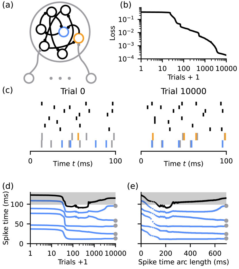
Figure 3: Learning precise spikes in an RNN. (a) Network schematic. Neurons receive in each trial the same spikes from external input neurons (gray). Recurrent weights and initial conditions are learned such that the first two network neurons (blue and orange) spike at desired times. (b) Loss dynamics during learning. (c) Left: Spikes of network neurons before learning. Spikes of the first two neurons are colored, their target times are displayed in gray. Right: Learning changes the network dynamics such that the first two neurons spike precisely at the desired values (the colored spikes mostly cover the gray ones). (d) Evolution of the spike times of the first neuron during learning. The times of the spikes that are supposed to lie within the trial (blue traces) shift towards their target values (gray circles). The next spike (black trace) is supposed to lie outside the trial. (Gray area indicates pseudospikes.) (e) Same as (d) but the spike times are shown as a function of the arc length of the output spike time trajectories. This demonstrates that the spike times change continuously, despite the occurrence of large gradients (c.f. the step-like change in (d)).

Next, we consider the training of a recurrent neural network (RNN). Successful learning of recurrent connections can be used for the construction of models of cortical networks, which are characterized by a high degree of recurrence [1], when the values of weights or other parameters are unknown [18, 38, 39]. In an RNN, spikes of all neurons generally influence subsequent spikes of all neurons. Thus, a change in a spike has a much broader and less straightforward impact than when training a single neuron. This renders RNN training harder.

We consider a fully-connected RNN of ten QIF neurons with extended coupling and external inputs. The spike times of two network neurons are learned (Fig. 3a). In contrast to the learning of all network spikes [40, 18], such a task does not reduce to multiple single neuron learning tasks. Similar to the previous task, we apply our spike-based gradient descent to minimize the quadratic difference between spike times and their targets. Both the recurrent weights and the initial conditions of the neurons are learned. The latter exemplifies that our scheme can be applied not only to weights and input spike times but also to further network parameters.

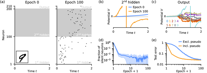
Figure 4: Spike-based gradient descent learning of the MNIST dataset. (a) Spike raster plot of the three-layer network. Left: It is silent before learning (inset shows example input also used on the right, and in b, c). Right: After learning, the neurons spike sparsely. (b) Voltage dynamics of the first neuron of the second hidden layer before (blue) and after (orange) learning. Despite not receiving any input before learning, our learning scheme adjusts upstream connection weights such that it eventually starts to spike. (c) Voltage dynamics of all output neurons after learning. Only the output neuron representing the correct class (“9”) spikes. (d) The fraction of neurons that do not spike before the first output spike for any input image quickly decays from (almost) one to a near zero value. (e) The networks achieve low test classification errors. If also pseudospikes are used for classification (orange), learning is faster. Horizontal gray lines in (b,c) indicate $V_{\text{rest}}$, black bars indicate potential difference of one. Solid lines in (d,e) indicate mean and shaded areas std over ten network instances.

Our scheme is successful also in this scenario (Fig. 3b,c). The spike times are learned with great precision, the maximal deviation of any of the learned spikes from its target time is less than 2. As in the previous example, the spike times of the first neuron change continuously during learning without discrete jumps of the spike times (Fig. 3d,e). Due to large gradients, which are typical for all kinds of RNNs [41], the spike times of the second neuron change seemingly jump-like (Supplemental Material Fig. S6). Such sudden changes can be smoothened by restricting the maximal spike time change per step with the help of adjustable update step sizes (Supplemental Material Fig. S7). Hence, the applicability of our scheme extends to multi-spike learning and recurrent networks.

IV.4 Solving a standard machine learning task

Finally, we apply our scheme to the classification of hand-written single-digit numbers from the MNIST dataset, which is a widely used benchmark in neuromorphic computing (e.g. [20, 24, 29]).

We employ a three-layer feed-forward network. For computational efficiency, we use oscillatory QIF neurons with infinitesimally short input currents. For each input pixel, there is a corresponding input neuron, which spikes once at the beginning of the trial if the binarized pixel intensity is one and otherwise remains silent. The input spikes are then further processed by two hidden layers of 100 neurons each. The index of the neuron in the output layer that spikes first is the model prediction. Such time-to-first-spike coding naturally leads to fast classification in terms of time and number of spikes. Hence, it is well suited to foster the potential advantages of neuromorphic hardware regarding energy-efficiency and inference time. From a biological perspective, there is experimental evidence that the first spikes of neurons encode sensory information [2, 42, 43].

To demonstrate that our scheme allows to solve the dead neuron problem even if neurons in multiple layers are silent, we randomly initialize network parameters such that there are initially basically no ordinary spikes (Fig. 4a, left). Concretely, 99.9 (mean over ten network instances, also in the following) of all hidden neurons initially do not generate ordinary spikes for any input image in the test data set. Yet, the pseudospike time-dependent, imposed interaction between the neurons allows to backpropagate errors. Hence, minimizing the cross-entropy loss activates the hidden (Fig. 4b) and output (Fig. 4c) neurons. The fraction of neurons that do not spike before the first output spike (where test trials can in principle be terminated) for any input image, quickly decays to a final value of 0.2 (Fig. 4d). This means nearly all hidden neurons are utilized for inference. Still, the activity after learning is sparse with $0.31$ ordinary spikes per hidden neuron before the first output spike, which is beneficial in terms of energy- and time-efficiency. The final accuracy of 97.3 when only considering ordinary output spikes is comparable to previous results where similar setups are considered [25, 23, 24, 44]. If we also allow pseudospikes in the classification, the accuracy does not change much, it becomes 97.5. The convergence to minimal error is, however, faster (Fig. 4d). Thus, our scheme achieves competitive performance in a neuromorphic benchmark task even if almost no neuron is initially active (see Supplemental Material Sec. VI for further quantitative measures).

V Discussion

We have shown that there are neural networks with spike times that vary continuously or even smoothly with network parameters; ordinary spikes only (dis-)appear at the end of the trial and can be extended to pseudospikes. The networks allow to learn the timings of an arbitrary number of spikes in a continuous fashion with a spike-based gradient.

Perhaps surprisingly, the networks may consist of rather simple, standard QIF neurons. These are widely used in theoretical neuroscience [31, 6], including for the supervised learning of spiking neural networks [38, 45, 46]. However, the particularity that spikes only (dis-)appear at the trial end has not been noticed and exploited. Furthermore, QIF neurons have already been implemented in neuromorphic hardware [47, 48].

On the one hand, our scheme possesses the same advantages as other spike-based gradient descent approaches such as small memory and computational footprints and a clear interpretation as following the exact loss gradient. On the other hand, like standard machine learning schemes it produces no disruptive transitions during learning and no gradient divergences; it can in principle be used with any type of initialization and does not rely on ad-hoc measures to remove and add spikes and revive dead neurons. This suggests a wide range of applications: When studying biological neural networks, our scheme may be used to learn neurobiologically relevant tasks, in order to benchmark biological learning and to investigate how the network dynamical solutions may work. The scheme may also be used to reconstruct synaptic connectivity from experimentally (partially) observed spiking activity. Furthermore, it may be used to train networks in neuromorphic computing. It generally allows to benchmark other learning rules whose underlying mechanisms are less transparent and to (pre-)train networks before converting to a desired neuron type that complicates learning.

The dynamics of spiking and non-spiking neural networks can have long temporal dependencies with small perturbations increasing over time [49, 50, 51, 52, 35], see also Supplementary Material Sec. IV. For learning this causes the well-known exploding gradient problem [10, 41]. We therefore restricted our learning examples to at most ten multiples of the membrane time constant. This fits the length of various experimentally observed precisely timed patterns of spikes [53, 42, 2, 54, 55, 56] and the fast processing of certain tasks in neuromorphic computing [20, 25, 23, 24, 44].

We have introduced pseudospikes to allow the gradient to “see” spikes before they appear and to thus add spikes in systematic manner. This preserves the gradients of the ordinary spike times and solves, in particular, the dead neuron problem. The resulting possibility to initialize an entire network with small weights may be important to induce desirable and biologically plausible features such as energy-efficient final connectivity and sparse spiking [57, 7], sparse coding [58] and representation learning [59]. In a somewhat related approach, silent neurons were assumed to spike at the trial end [26, 27]. In contrast to our pseudospikes, however, this only applied to output neurons and did not allow to backpropagate errors through silent neurons.

To conclude, the present study shows that despite the inherent discreteness of spikes, it is possible to perform exact, smooth gradient descent in spiking neural networks, including the gradient-based removal and after augmentation also generation of spikes.