Byzantine-Resilient Federated Principal Subspace Estimation and Applications in PCA and Low Rank Matrix Recovery

Byzantine-Resilient Federated PCA and Low Rank Matrix Recovery

Abstract

In this work we consider the problem of estimating the principal subspace (span of the top $r$ singular vectors) of a symmetric matrix in a federated setting, when each node has access to estimates of this matrix. We study how to make this problem Byzantine resilient. We introduce a novel provably Byzantine-resilient, communication-efficient, and private algorithm, called Subspace-Median, to solve it. We also study the most natural solution for this problem, a geometric median based modification of the federated power method, and explain why it is not useful. We consider two special cases of the resilient subspace estimation meta-problem - federated principal components analysis (PCA) and the spectral initialization step of horizontally federated low rank column-wise sensing (LRCCS) in this work. For both these problems we show how Subspace Median provides a resilient solution that is also communication-efficient. Median of Means extensions are developed for both problems. Extensive simulation experiments are used to corroborate our theoretical guarantees. Our second contribution is a complete AltGDmin based algorithm for Byzantine-resilient horizontally federated LRCCS and guarantees for it. We do this by developing a geometric median of means estimator for aggregating the partial gradients computed at each node, and using Subspace Median for initialization.

I Introduction

In this work we develop provably Byzantine resilient algorithms for solving federated principal components analysis (PCA) and related problems. Federated learning is a setting where multiple entities/nodes/clients collaborate in solving a machine learning (ML) problem. Each node can communicate with a central server or service provider. Each node/client’s raw data is stored locally and not exchanged or transferred. Summaries of it are shared with the central server which aggregates all of them and broadcasts an aggregate estimate to all the nodes [1]. One of the challenges in this setup is adversarial attacks on the clients. In this work we consider “Byzantine attacks”, defined in the general sense: the attacking nodes can collude and know the nodes’ outputs, the algorithm being implemented by the center and the algorithm parameters.

I-A Existing Work

There has been a large amount of recent work on Byzantine-resilient federated ML algorithms, some of which come with provable guarantees [2, 3, 4, 5, 6, 7, 8, 9, 10, 11, 12, 13, 14, 15, 16, 17, 7, 18, 5]. Some of the theoretical guarantees are asymptotic, and almost all of them analyze the standard gradient descent (GD) algorithm or stochastic GD.

Typical solutions involve replacing the mean of the gradients from the different nodes by a different robust statistic, such as geometric median (of means) [2], trimmed mean, coordinate-wise mean [4] or Krum [3].

One of the first non-asymptotic results for Byzantine attacks is [2]. This used the geometric median (GM) of means to replace the regular mean/sum of the partial gradients from each node. Under standard assumptions (strong convexity, Lipschitz gradients, sub-exponential-ity of sample gradients, and an upper bound on the fraction of Byzantine nodes), it provided an exponentially decaying bound on the distance between the estimate at the $t$-th iteration and the unique global minimizer. In follow-up work [4], the authors studied the coordinate-wise mean and the trimmed-mean estimators and developed guarantees for both convex and non-convex problems. Because this work used coordinate-wise estimators, the new results needed smoothness and convexity along each dimension. This is a stronger, and sometimes impractical, assumption. Another interesting series of works [6, 8] provides non-asymptotic guarantees for Byzantine resilient stochastic GD. This work develops an elaborate median based algorithm to detect and filter out the Byzantine nodes. The theoretical analysis assumes that the norm of the sample gradients is bounded by a constant (that does not depend on the gradient dimension). Consequently they are able to obtain sample complexity guarantees that do not depend on the signal dimension. These works also assume that the set of Byzantine nodes is the same for all GD iterations, while the work of [2] allowed this set to vary at each iteration.

Most of the above works considered the homogeneous data setting; this means that the data that is i.i.d. (independent and identically distributed) across all nodes. More recent work has focused on heterogeneous distributions (data is still independent across nodes but is not identically distributed) and proved results under upper bounds on the amount of heterogeneity [12, 13, 14, 15]. Other works rely on detection methods to handle heterogeneous gradients [16, 17, 7, 18, 5]. These assume the existence of a trustworthy root/validation dataset at the central server and that is used for detecting the adversarial gradients.

I-B Problem setting – Two Specific Problems and the Meta Problem – and Notation

I-B1 Two specific problems

We consider two related problems in this work. The first is Byzantine-resilient federated PCA with data vertically federated on $L$ nodes. Given $q$ data vectors $\bm{d}_{k}\in\Re^{n}$, that are zero mean, mutually independent and identically distributed (i.i.d.), the goal of PCA is to find the $r$-dimensional principal subspace (span of top $r$ singular/eigen vectors) of their covariance matrix, which we will denote by $\bm{\Sigma}^{*}$. We can arrange the data vectors into an $n\times q$ matrix, $\bm{D}:=[\bm{d}_{1},\bm{d}_{2},\dots\bm{d}_{q}]$. Vertical federation means that a $q_{\ell}=q/L$ column sub-matrix of $\bm{D}$, denoted $\bm{D}_{\ell}$, is observed at node $\ell$, and $\bm{D}=[\bm{D}_{1},\bm{D}_{2},\dots,\bm{D}_{\ell},\dots,\bm{D}_{L}]$. We are assuming that $q$ is a multiple of $L$.

The second problem is low rank column-wise compressive sensing (LRCCS) in a horizontally federated setting while being robust to Byzantine attacks. LRCCS involves recovering an $n\times q$ rank-$r$ matrix $\bm{X}^{*}$ from compressive linear measurements of each column, i.e., from $\bm{y}_{k}:=\bm{A}_{k}\bm{x}^{*}_{k}$, $k\in[q]$, with $\bm{y}_{k}\in\Re^{m}$ with $m\ll n$, and $\bm{A}_{k}$ being $m\times n$ matrices which are i.i.d. random Gaussian (each entry is i.i.d. standard Gaussian) [19]. We treat $\bm{X}^{*}$ as a deterministic unknown. Here and below $[q]:=\{1,2,\dots,q\}$. This problem is also sometimes referred to as “compressive PCA”. Let $\bm{Y}=[\bm{y}_{1},\bm{y}_{2},\dots,\bm{y}_{q}]$. Horizontal federation means that row sub-matrices of $\bm{Y}$ are observed at the different nodes. In [19], we developed a GD based algorithm, called alternating GD and minimization (AltGDmin), for solving the LRCCS problem in a fast and communication-efficient fashion. AltGDmin needs to be initialized by computing the top $r$ singular vectors of a matrix that we specify later (spectral initialization). If this step works reliably, the rest of the AltGDmin algorithm can be made Byzantine resilient by adapting the approach of [2] to our setting. We explain this in Section V-A.

Two applications where the LRCCS problem occurs are accelerated dynamic MRI and federated sketching [20, 21]. In multicoil dynamic MRI, rows of the data matrix $\bm{Y}$ are acquired at different nodes.

The reason we consider vertical federation for PCA but horizontal for LRCCS is because these are the settings in which the data on the different nodes is i.i.d. in each case. In case of vertically federated PCA, $\bm{D}_{\ell}$’s are i.i.d. If we consider horizontal federation for PCA, then this is no longer true (unless we assume $\bm{\Sigma}^{*}$ is block diagonal). For LRCCS, the opposite holds because different entries of a given $\bm{y}_{k}$ are i.i.d.; but the different $\bm{y}_{k}$’s are not identically distributed. Guaranteeing Byzantine resilience without extra assumptions requires the different nodes’ data be i.i.d. or i.i.d.-like.

I-B2 The meta problem

Both problems above – Byzantine-resilient federated PCA and the initialization step for LRCCS – can be interpreted as special cases of the following meta problem. We need to find the subspace spanned by the top $r$ singular vectors of a symmetric $n\times n$ matrix, $\bm{\Phi}^{*}$. Denote the $n\times r$ matrix formed by these singular vectors by ${\bm{U}}^{*}$. Our goal is to estimate $span({\bm{U}}^{*})$. Each node $\ell$ observes an $n\times q_{\ell}$ data matrix $\bm{D}_{\ell}$ that is such that $\bm{\Phi}_{\ell}:=\bm{D}_{\ell}\bm{D}_{\ell}^{\top}/q_{\ell}$ is an estimate of $\bm{\Phi}^{*}$. We use $\sigma_{1}^{*}\geq...\geq\sigma_{n}^{*}$ to denote the singular values of $\bm{\Phi}^{*}$. We assume that at most $\tau L$ nodes are Byzantine for a $\tau<0.4$. The federated setting requires the algorithm to be communication-efficient and private. Here private means that the center should not have access to the nodes’ raw data.

I-B3 Notation

We use $\|.\|_{F}$ to denote the Frobenius norm and $\|.\|$ without a subscript to denote the (induced) $l_{2}$ norm (often called the operator norm or spectral norm); ^⊤ denotes matrix or vector transpose; $|\bm{z}|$ for a vector $\bm{z}$ denotes element-wise absolute values; $\bm{I}_{n}$ (or sometimes just $\bm{I}$) denotes the $n\times n$ identity matrix, and $\bm{e}_{k}$ denotes its $k$-th column ($k$-th canonical basis vector); and $\bm{M}^{\dagger}=(\bm{M}^{\top}\bm{M})^{-1}\bm{M}^{\top}$. We use $\mathbb{1}_{\{a\leq b\}}$ to denote the indicator function that returns $1$ if $a\leq b$ otherwise $0$.

We use $QR({\bm{U}})$ to denote the orthonormalization of the columns of ${\bm{U}}$ by using QR decomposition. We use $SVD_{r}(\bm{D})$ ($r$-SVD) to refer to the top $r$ left singular vectors (singular vectors corresponding to the $r$ largest singular values) of the matrix $\bm{D}$. If the matrix is symmetric and positive semi-definite, these are also the top eigenvectors. The projection matrix for projecting onto $span({\bm{U}})$ (the subspace spanned by the columns of ${\bm{U}}$) is denoted $\mathcal{P}_{\bm{U}}:={\bm{U}}{\bm{U}}^{\top}$ while that for projecting orthogonal to $span({\bm{U}})$ is denoted $P_{{\bm{U}},\perp}:=\bm{I}-{\bm{U}}{\bm{U}}^{\top}$

For tall matrices with orthonormal columns ${\bm{U}}_{1},{\bm{U}}_{2}$, we use $\bm{SD}_{F}({\bm{U}}_{1},{\bm{U}}_{2}):=\|(\bm{I}-{\bm{U}}_{1}{\bm{U}}_{1}{}^{\top}){\bm{U}}_{2}\|_{F}$ as the default Subspace Distance (SD) measure between the subspaces spanned by the two matrices. In some places, we also use $\bm{SD}_{2}({\bm{U}}_{1},{\bm{U}}_{2})=\|(\bm{I}-{\bm{U}}_{1}{\bm{U}}_{1}{}^{\top}){\bm{U}}_{2}\|$. If both matrices have $r$ columns (denote $r$-dimensional subspaces), then $\bm{SD}_{F}({\bm{U}}_{1},{\bm{U}}_{2})\leq\sqrt{r}\bm{SD}_{2}({\bm{U}}_{1},{\bm{U}}_{2})$.

We reuse the letters $c,C$ to denote different numerical constants in each use with the convention that $c<1$ and $C\geq 1$. Also the notation $a\lesssim b$ means $a\leq Cb$.

We use $\mathcal{J}_{good}\subseteq[L]$ to denote the set of indices of the good (non-Byzantine) nodes.

When computing a median of means estimator, one splits the $L$ node indices into $\tilde{L}$ mini-batches so that each mini-batch contains $\rho=L/\tilde{L}$ indices. For the $\ell$-th node in the $\vartheta$-th mini-batch we use the short form notation ${(\vartheta,\ell)}={(\vartheta-1)\rho+\ell}$, for $\ell\in[\rho]$.

For $a,b$ in $(0,1)$, we use $\psi(a,b):=(1-a)\log\frac{1-a}{1-b}+a\log\frac{a}{b}$ to denote the binary KL divergence.

I-C Contribution

Our first contribution is a novel provably Byzantine-resilient, communication-efficient, and private algorithm, that we refer to as “Subspace-Median”. This helps estimate the principal subspace (span of the top $r$ singular vectors) of a symmetric matrix in a federated setting, when each node has access to estimates of this matrix. The performance, communication-complexity and time-complexity guarantees for this algorithm are provided in Theorem 3.6. We also study the most natural solution for this problem, a GM-based modification of the federated power method, and explain why it is not useful; see Theorem 3.5 and the discussion below it. Next, we show how Subspace-Median provides a Byzantine resilient solution for two different problems. The first is federated PCA and the second is the spectral initialization step of horizontally federated LRCCS. We develop Subspace Median of Means extensions for both problems. These help improve the sample complexity at the cost of reduced Byzantine/outlier tolerance. For all these algorithms, Theorem 3.6 helps prove sample, communication, and time complexity bounds for $\epsilon$-accurate subspace recovery. Extensive simulation experiments are used to corroborate our theoretical results. Our second contribution is a complete AltGDmin based algorithm for Byzantine-resilient horizontally federated LRCCS and guarantees for it. We do this by developing a geometric median of means estimator for aggregating the partial gradients computed at each node, and combining its guarantee with that for spectral initialization (obtained as a corollary of Theorem 3.6).

One component that is missing in most existing work on Byzantine resiliency is how to initialize the GD algorithm for a non-convex problem in such a way that the problem becomes restricted strongly convex in its vicinity. Most works either consider globally strongly convex cost functions or prove convergence to a local minimum value. But good initialization is a critical component for correctly solving most low-rank, or low-rank plus sparse, matrix recovery problems. Most such algorithms are initialized using a spectral initialization, which requires subspace estimation. To our best knowledge, there is no existing provable solution for Byzantine resilient federated PCA or subspace estimation. Thus, our algorithm and its proof techniques are likely to be of independent interest for other problems as well.

We explain the novelty of our algorithmic and proof techniques and provide a detailed discussion of where else these might be useful in Sec. VII.

I-D Organization

We define the geometric median (GM), explain how to compute it, and how to use it for robust estimation in Sec. II. We introduce the Subspace Median solution, and its guarantee, for the resilient subspace estimation meta-problem in Sec. III. This section also explains why other obvious solutions to this problem are not useful. We use the Subspace Median algorithm to develop a basic solution for Byzantine-resilient federated PCA in Sec. IV. In this section, we also develop a Subspace Median-of-Means solution. In Sec. V, we consider the LRCCS problem in a horizontally federated setting. We first use the Subspace Median algorithm to develop a Median and Median-of-Means solution for its initialization. Next, we also develop a GM of means based modification of the AltGDmin algorithm itself. Simulation experiments are provided in Sec. VI. We conclude with a discussion of our proof techniques, potential extensions of this work, and of the open questions in Sec. VII.

II Geometric Median Preliminaries

II-A Geometric median (GM) and its computation

Geometric median (GM) is one way to define a median of vectors. For $L$ vectors, $\mathcal{A}=\{\bm{z}_{1},\bm{z}_{2},...,\bm{z}_{L}\}\subseteq\Re^{n}$, it is defined as

$$GM\{\bm{z}_{1},\bm{z}_{2},...,\bm{z}_{L}\}=\arg\min_{\bm{z}\in\Re^{n}}\sum_{\ell=1}^{L}\left\|\bm{z}-\bm{z}_{\ell}\right\|$$

This problem cannot be solved in closed form. Iterative algorithms exist to solve it approximately. When we say $\bm{z}_{gm}$ is a $(1+\epsilon_{0})$ approximate GM we mean that

$$\sum_{\ell=1}^{L}\left\|\bm{z}_{gm}-\bm{z}_{\ell}\right\|\leq(1+\epsilon_{0})\min_{\bm{z}\in\Re^{n}}\sum_{\ell=1}^{L}\left\|\bm{z}-\bm{z}_{\ell}\right\|$$

There are two popular iterative solutions for computing the approximate GM. The first, and most commonly used one in practice, is Weiszfeld’s algorithm initialized using the average of the $\bm{z}_{\ell}$’s [22]. However this only comes with an asymptotic guarantee which cannot be used to bound its iteration complexity (number of iterations required to obtain a certain error level). Consequently, we cannot bound its time complexity. Weiszfeld’s algorithm with a different (somewhat complicated) initialization is studied in [23]. This gives an iteration complexity bound. But the bound depends on algorithm parameters and the quantities used to define the initialization in a way that it is impossible/difficult to further bound it in terms of only model parameters. Because of this, we cannot use Weiszfeld’s method to obtain a useful bound on its computational complexity. The second solution is the algorithm studied in Cohen et al [24]. This comes with a simple time complexity guarantee which we provide next.

Theorem 2.1 (Theorem 1 [24]).

Consider [24, Algorithm 1] (provided in our Appendix in Algorithm 7). With constant probability, $1-c_{0}$ (with $c_{0}<1$ being a numerical constant), it obtains a $(1+\epsilon_{gm})$-approximate geometric median in order $T_{gm}=C\log(\frac{L}{\epsilon_{gm}})$ iterations. Its per iteration complexity is $CLn\log^{2}(\frac{L}{\epsilon_{gm}}))$. Thus, its total time complexity is $O(Ln\log^{3}(\frac{L}{\epsilon_{gm}}))$.

Although it has a simple guarantee, the algorithm [24, Algorithm 1] is complicated. Even the authors of this work itself have not shown any experimental results with it. To our best knowledge, nor have any other authors in follow-up work that cites it. We provide both this algorithm and Weiszfeld’s method (and the two guarantees for it) in Appendix E.

In this work, for our theoretical guarantees we will assume that [24, Algorithm 1] is used. In our simulation experiments, we use Weiszfeld’s algorithm initialized using the average of the $\bm{z}_{\ell}$’s.

II-B Using GM for robust estimation

In robust estimation, the goal is to get a good estimate of a vector quantity $\tilde{\bm{z}}$ using $L$ individual estimates of it, denoted $\bm{z}_{\ell}$, when most of the estimates are good, but a few can be arbitrarily corrupted or modified by Byzantine attackers. A good approach to do this is to use the GM. The following lemma, borrowed from [2], studies this.

Lemma 2.2.

Let $\mathcal{A}=\{\bm{z}_{1},...,\bm{z}_{L}\}$ with each $\bm{z}_{\ell}\subseteq\Re^{n}$ and let $\bm{z}_{gm}$ denote their $(1+\epsilon_{gm})$ approximate GM estimate. Fix an $\alpha\in(0,1/2)$. Suppose that the following holds for estimates from at least $(1-\alpha)L$ nodes: $\|\bm{z}_{\ell}-\tilde{\bm{z}}\|\leq\epsilon\|\tilde{\bm{z}}\|$.

Then, w.p. at least $1-c_{0}$,

$$\|\bm{z}_{gm}-\tilde{\bm{z}}\| \leq C_{\alpha}\epsilon\|\tilde{\bm{z}}\|+\epsilon_{gm}\frac{\sum_{\ell=1}^{L}\|\bm{z}^{*}-\bm{z}_{\ell}\|}{(1-2\alpha)L}$$

$$\leq C_{\alpha}\epsilon\|\tilde{\bm{z}}\|+\epsilon_{gm}\frac{\max_{\ell\in[L]}\|\bm{z}_{\ell}\|}{1-2\alpha}$$

where $C_{\alpha}:=\frac{2(1-\alpha)}{1-2\alpha}$.

To understand this lemma simply, fix the value $\alpha$ to 0.4. Then $C_{\alpha}=6$. We can also fix $\epsilon_{gm}=\epsilon$. Then, it says the following. If at least 60% of the $L$ estimates are $\epsilon$ close to $\tilde{\bm{z}}$, then, the $(1+\epsilon)$ approximate GM, $\bm{z}_{gm}$, is $11\epsilon\max(\|\tilde{\bm{z}}\|,\max_{\ell}\|\bm{z}_{\ell}\|)$ close to $\tilde{\bm{z}}$. The next lemma follows using the above lemma and is a minor modification of [2, Lemma 3.5]. It fixes $\alpha=0.4$ and considers the case when most estimates are good with high probability (whp).

Lemma 2.3.

Let $\mathcal{A}=\{\bm{z}_{1},...,\bm{z}_{L}\}$ with each $\bm{z}_{\ell}\subseteq\Re^{n}$, and let $\bm{z}_{gm}$ denote a $(1+\epsilon_{gm})$ approximate GM. For a $\tau<0.4$, suppose that, for at least $(1-\tau)L$ $\bm{z}_{\ell}$’s,

$$\Pr\{\|\bm{z}_{\ell}-\tilde{\bm{z}}\|\leq\epsilon\|\tilde{\bm{z}}\|\}\geq 1-p$$

Then, w.p. at least $1-c_{0}-\exp(-L\psi(0.4-\tau,p))$,

$$\|\bm{z}_{gm}-\tilde{\bm{z}}\|\leq 6\epsilon\|\tilde{\bm{z}}\|+5\epsilon_{gm}\max_{1\leq i\leq L}\|\bm{z}_{\ell}\|$$

where $\psi(a,b)=(1-a)\log\frac{1-a}{1-b}+a\log\frac{a}{b}$.

Furthermore, if $\|\bm{z}_{\ell}\|\leq\|\tilde{\bm{z}}\|$, then $\|\bm{z}_{gm}-\tilde{\bm{z}}\|\leq 11\epsilon\|\tilde{\bm{z}}\|$ with above probability. The number of iterations needed is $T_{gm}=C\log(\frac{L}{\epsilon_{gm}})$, and the time complexity is $O\left(nL\log^{3}(\frac{L}{\epsilon_{gm}})\right)$.

Suppose that, for a $\tau<0.4$, at least $(1-\tau)L$ $\bm{z}_{\ell}$s are “good” (are $\epsilon$ close to $\tilde{\bm{z}}$) whp. Let $\epsilon_{gm}=\epsilon$ and suppose that all $\bm{z}_{\ell}$’s, including the corrupted ones, are bounded in 2-norm by $\|\tilde{\bm{z}}\|$. Then, the $(1+\epsilon)$-approximate GM is about $11\epsilon\|\tilde{\bm{z}}\|$ close to $\tilde{\bm{z}}$ with at least constant probability. If the GM is approximated with probability 1, i.e., if $c_{0}=0$, then, the above result says that, for $p$ small enough and large $L$, the reliability of the GM is actually higher than that of the individual good estimates. For example, for a $p<0.01$, the probability is at least $1-p^{L(0.4-\tau)}$. The increase depends on $(0.4-\tau)$ and $L$, e.g., if $\tau\geq 0.2$ and $L\geq 10$, then, the probability is at least $1-p^{0.2L}\geq 1-p^{2}$.

II-C Using the above result for unbounded $\bm{z}_{\ell}$s

In settings where all $\bm{z}_{\ell}$’s are bounded, the above result is directly applicable. When they are not bounded, we need an extra thresholding step. Observe that, from the lemma assumption, w.p. at least $1-Lp$, the good $\bm{z}_{\ell}$’s are bounded by $(1+\epsilon)\|\tilde{\bm{z}}\|$. Thus, to get a bounded set of $\bm{z}_{\ell}$’s while not eliminating any of the good ones, we can create a new set $\mathcal{A}_{thresh}$ that only contains $\bm{z}_{\ell}$s with norm smaller than threshold $\omega=(1+\epsilon)\|\tilde{\bm{z}}\|$, i.e., we use $\mathcal{A}_{thresh}=\{\bm{z}_{1},...,\bm{z}_{L}\}\setminus\{\bm{z}_{\ell}:\|\bm{z}_{\ell}\|>(1+\epsilon)\|\tilde{\bm{z}}\|\}$ as the input to the GM computation algorithm [24, Algorithm 1]. We have the following corollary of Lemma 2.4 for this setting.

Lemma 2.4.

Let $\bm{z}_{gm}$ denote a $(1+\epsilon_{gm})$ approximate GM of $\{\bm{z}_{1},...,\bm{z}_{L}\}\setminus\{\bm{z}_{\ell}:\|\bm{z}_{\ell}\|>\omega\}$, all vectors are in $\Re^{n}$. Set $\omega=(1+\epsilon)\|\tilde{\bm{z}}\|$. For a $\tau<0.4$, suppose that, for at least $(1-\tau)L$ $\bm{z}_{\ell}$’s,

$$\Pr\{\|\bm{z}_{\ell}-\tilde{\bm{z}}\|\leq\epsilon\|\tilde{\bm{z}}\|\}\geq 1-p$$

Then, w.p. at least $1-c_{0}-Lp-\exp(-L\psi(0.4-\tau,p))$,

$$\|\bm{z}_{gm}-\tilde{\bm{z}}\|\leq 6\epsilon\|\tilde{\bm{z}}\|+5\epsilon_{gm}(1+\epsilon)\|\tilde{\bm{z}}\|<14\max(\epsilon,\epsilon_{gm})\|\tilde{\bm{z}}\|$$

The number of iterations needed is $T_{gm}=C\log(\frac{L}{\epsilon_{gm}})$, and the time complexity is $O\left(nL\log^{3}(\frac{L}{\epsilon_{gm}})\right)$.

III Resilient federated subspace estimation

Recall that our goal is to obtain a communication-efficient and private algorithm to estimate the subspace, $span({\bm{U}}^{*})$, spanned by the top $r$ singular vectors of a symmetric $n\times n$ matrix $\bm{\Phi}^{*}$. We consider a federated setting in which each node $\ell$ has, or can compute, a symmetric matrix $\bm{\Phi}_{\ell}$ which is an estimate of $\bm{\Phi}^{*}$. In both the applications we consider in this work, the node has access to an $n\times q_{\ell}$ data matrix $\bm{D}_{\ell}$ and $\bm{\Phi}_{\ell}=\bm{D}_{\ell}\bm{D}_{\ell}^{\top}/q_{\ell}$. In the first case, $q_{\ell}=\widetilde{q}:=q/L$ while for the second one $q_{\ell}=q$. We assume that at most $\tau L$ nodes are Byzantine for a $\tau<0.4$.

Algorithm 1 Resilient Power Method - a bad solution

Parameters $T_{pow}$, $T_{gm}$, $\omega$

1:  Central Server Randomly Initialize ${\bm{U}}_{rand}$ with i.i.d standard Gaussian entries. Set ${\bm{U}}_{0}={\bm{U}}_{rand}$.

2:  for $t\in T_{pow}$ do

3:     Nodes $\ell=1,...,L$

4:     Compute $\bm{\Phi}_{\ell}{\bm{U}}_{t-1}$

5:     Central Server

6:     $GM\leftarrow approxGMthresh\{\bm{\Phi}_{\ell}{\bm{U}}_{t-1},\ \ell\in[L]\}$ (Use [24, Algorithm 1] with $T_{gm}$ iterations on $\{\bm{\Phi}_{\ell}{\bm{U}}_{t-1},\ \ell\in[L]\}\setminus\{\ell:\|\bm{\Phi}_{\ell}{\bm{U}}_{t-1}\|>\omega\}$)

7:     Orthonormalize: using QR $GM\stackrel{{\scriptstyle QR}}{{=}}\hat{{\bm{U}}}\bm{R}$

8:     Return ${\bm{U}}_{t}\leftarrow\hat{{\bm{U}}}$

9:  end for

10:  Output ${\bm{U}}_{out}\leftarrow{\bm{U}}_{T_{pow}}$

III-A Two bad solutions: Share Raw Data and Resilient Power Method (ResPowMeth)

The simplest way to deal with Byzantine attacks is to compute the GM of the vectorized matrices $\bm{\Phi}_{\ell}$ followed by computing the principal subspace ($r$-SVD) of the GM matrix. This solution was studied for PCA in [25]. However, in a federated setting, this is neither communication-efficient nor private because it requires the nodes to share $\bm{\Phi}_{\ell}$s with the center (to compute their GM).

For a communication-efficient and private solution, in the absence of attacks, we would use a federated version of the power method [26, 27]. With attacks, the most obvious solution would be a geometric median (GM) based modification of this algorithm. We refer to this as Resilient Power Method (ResPowMeth) and summarize it in Algorithm 1. However, this is not useful because, as the following guarantee shows, it requires all the $\bm{\Phi}_{\ell}$s to be extremely accurate estimates of $\bm{\Phi}^{*}$.

Theorem 3.5 (ResPowMeth guarantee).

Assume that at most $\tau L$ nodes are Byzantine with $\tau<0.4$. Assume also that $\sigma_{r}^{*}-\sigma_{r+1}^{*}\geq\Delta$ for a $\Delta>0$. Consider ResPowMeth (Algorithm 1) with $T_{pow}=C\frac{\sigma_{r}^{*}}{\Delta}\log(\frac{n}{\epsilon})$, $T_{gm}=\log\left(\frac{Lnr}{\epsilon}\right)$, and $\omega=1.1\sigma_{1}^{*}\sqrt{r}$. If, for all $\ell\in\mathcal{J}_{good}$,

$$\Pr\left\{\|\bm{\Phi}_{\ell}-\bm{\Phi}^{*}\|\leq\frac{1}{70}\min\left(\frac{\epsilon}{\sqrt{r}},\frac{1}{2nr}\right)\Delta\right\}\geq 1-p$$

then w.p. at least $1-c_{0}-Lp-\exp(-L\psi(0.4-\tau,p))-\frac{2}{\sqrt{n}}$,

$$\bm{SD}_{F}({\bm{U}}_{out},{\bm{U}}^{*})\leq\epsilon$$

The communication cost is $nrT_{pow}=Cnr\frac{\sigma_{r}^{*}}{\Delta}\log(\frac{n}{\epsilon})$ per node. The computational cost at the center is $nrLT_{gm}\cdot T_{pow}=nrL\frac{\sigma_{r}^{*}}{\Delta}\log^{3}\left(\frac{Lnr}{\epsilon}\right)\log(\frac{n}{\epsilon})$. The computational cost at any node is $nq_{\ell}rT_{pow}=nq_{\ell}r\frac{\sigma_{r}^{*}}{\Delta}\log(\frac{n}{\epsilon})$.

Proof.

This follows by using the GM result, Lemma 2.4, to bound $\|GM\{\bm{\Phi}_{\ell}{\bm{U}}\}_{\ell=1}^{L}-\bm{\Phi}^{*}{\bm{U}}\|_{F}$ followed by interpreting ResPowMeth as an instance of the noisy power method studied in [28]. We apply [28, Corollary 1] with $\bm{G}_{t}=\bm{\Phi}^{*}{\bm{U}}-GM\{\bm{\Phi}_{\ell}{\bm{U}}\}_{\ell=1}^{L}$. The proof is given in Appendix A-A.∎

Observe that the guarantee needs $\|\bm{\Phi}_{\ell}-\bm{\Phi}^{*}\|\lesssim\min(\epsilon/\sqrt{r},1/(nr))\cdot\Delta$ where $\Delta$ is a lower bound on the singular value gap (difference between the $r$-th and $(r+1)$-th singular values of $\bm{\Phi}^{*}$). The factor of $1/nr$ makes this requirement very stringent. For example, even to get an $\epsilon=0.1$ accurate subspace estimate, we need $\|\bm{\Phi}_{\ell}-\bm{\Phi}^{*}\|\lesssim\Delta/nr$.

To our best knowledge, it is not possible to improve the above bound even by directly analyzing the algorithm (we provide this analysis in Appendix F). Briefly the reason is that the power method is initialized randomly; for large $n,r$ a random subspace is a bad approximation of a given subspace $span({\bm{U}}^{*})$; and ResPowMeth computes the GM at each iteration including the first one .

We should mention that the above discussion is only based on required sufficient conditions. We have not proved that, if the required upper bound does not hold, the subspace estimation error is lower bounded by a large value. However, we do demonstrate this using extensive simulation experiments. For example, see Table II. In most cases, the error of ResPowMeth decreases very slightly whether we use $T_{pow}=1$ or $T_{pow}=10$.

Algorithm 2 Subspace Median

Input $\bm{\Phi}_{\ell}$, $\ell\in[L]$.
    Parameters $T_{gm}$, $T_{pow}$

1:  Nodes $\ell=1,...,L$

2:  Compute top $r$ singular vectors, $\hat{\bm{U}}_{\ell}$, of $\bm{D}_{\ell}$ (equivalently of $\bm{\Phi}_{\ell}:=\bm{D}_{\ell}\bm{D}_{\ell}^{\top}$). (Can use power method with $T_{pow}$ iterations)

3:  Central Server

4:  Orthonormalize: ${\bm{U}}_{\ell}\leftarrow QR(\hat{\bm{U}}_{\ell})$, $\ell\in[L]$

5:  Compute Projection Matrices: $\mathcal{P}_{{\bm{U}}_{\ell}}\leftarrow{\bm{U}}_{\ell}{\bm{U}}_{\ell}^{\top}$, $\ell\in[L]$

6:  Compute their GM: $\mathcal{P}_{GM}\leftarrow approxGM\{\mathcal{P}_{{\bm{U}}_{\ell}},\ \ell\in[L]\}$ (Use [24, Algorithm 1] with parameter $T_{gm}$).

7:  Find $\ell_{best}=\arg\min_{\ell}\|\mathcal{P}_{{\bm{U}}_{\ell}}-\mathcal{P}_{GM}\|_{F}$

8:  Output ${\bm{U}}_{out}={\bm{U}}_{\ell_{best}}$

III-B Proposed Solution: Subspace-Median (SubsMed)

As explained above, the resilient power method is not useful, and hence we need a better solution. We propose the following approach that we refer to as “Subspace-Median" (SubsMed). This relies on the following two simple facts: (i) In order to use the geometric median for matrices, we need a bound on the Frobenius norm between each non-Byzantine (good) matrix and the true one. (ii) The Frobenius norm between the projection matrices of two subspaces is a measure of subspace distance, i.e., $\|\mathcal{P}_{\bm{U}}-\mathcal{P}_{{\bm{U}}^{*}}\|_{F}=\sqrt{2}\bm{SD}_{F}({\bm{U}},{\bm{U}}^{*})$.

Our proposed algorithm, summarized in Algorithm 2, uses these facts. It proceeds as follows. Each node computes the top $r$ singular vectors of its matrix $\bm{\Phi}_{\ell}$, denoted $\hat{\bm{U}}_{\ell}$, and sends these to the center. If node $\ell$ is good, then $\hat{\bm{U}}_{\ell}$ already has orthonormal columns; however if the node is Byzantine, then it is not. The center first orthonormalizes the columns of all the received $\hat{\bm{U}}_{\ell}$’s using QR. This ensures that all the ${\bm{U}}_{\ell}$’s have orthonormal columns. It then computes the projection matrices $\mathcal{P}_{{\bm{U}}_{\ell}}:={\bm{U}}_{\ell}{\bm{U}}_{\ell}^{\top}$, $\ell\in[L]$, followed by vectorizing them and computing their GM. Denote the GM by $\mathcal{P}_{GM}$.

Finally, the center finds the $\ell$ for which $\mathcal{P}_{{\bm{U}}_{\ell}}$ is closest to $\mathcal{P}_{GM}$ in Frobenius norm and outputs the corresponding ${\bm{U}}_{\ell}$.

We should mention that this last step can also be replaced by finding the top $r$ singular vectors of $\mathcal{P}_{GM}$. However, doing this requires time of order $n^{2}r\log(1/\epsilon)$ while finding the closest $\mathcal{P}_{{\bm{U}}_{\ell}}$ only needs time of order $\max(n^{2},L\log L)$.

For the above approach to give an $\epsilon$-accurate subspace estimate (in Frobenius norm SD), as we show next, we need the estimates $\bm{\Phi}_{\ell}$ to be order $\epsilon/\sqrt{r}$ accurate. This is a much easier requirement to satisfy than what ResPowMeth needs. Moreover, SubsMed is even more communication efficient than ResPowMeth because the nodes need to send ${\bm{U}}_{\ell}$’s of size $n\times r$ only once. We discuss its computational cost after stating our guarantee for it.

Theorem 3.6 (Subspace-Median guarantee).

Assume that at most $\tau L$ nodes are Byzantine, i.e., that $|\mathcal{J}_{good}|\geq(1-\tau)L$, with $\tau<0.4$. Assume also that $\sigma_{r}^{*}-\sigma_{r+1}^{*}\geq\Delta$ for a $\Delta>0$. Assume that, for all $\ell\in\mathcal{J}_{good}$,

$$\Pr\left\{\|\bm{\Phi}_{\ell}-\bm{\Phi}^{*}\|\leq\frac{\epsilon}{92\sqrt{r}}\Delta\right\}\geq 1-p.$$

1. Consider Algorithm 2 with $T_{gm}=C\log\left(\frac{Lr}{\epsilon}\right)$ and use of exact SVD at the nodes. Then, w.p. at least $1-c_{0}-\exp(-L\psi(0.4-\tau,p))$,

   $$\bm{SD}_{F}({\bm{U}}_{out},{\bm{U}}^{*})\leq\epsilon$$

2. Consider Algorithm 2 with $T_{gm}$ as above and with the nodes using power method with $T_{pow}=C\frac{\sigma_{r}^{*}}{\Delta}\log(\frac{n}{\epsilon})$. Then, w.p. at least $1-c_{0}-\exp(-L\psi(0.4-\tau,p+\frac{1}{n^{10}}))$,

   $$\bm{SD}_{F}({\bm{U}}_{out},{\bm{U}}^{*})\leq\epsilon$$

   The communication cost is $nr$ per node. The computational cost at the center is order $n^{2}L\log^{3}\left(\frac{Lr}{\epsilon}\right)$. The computational cost at any node is order $nq_{\ell}rT_{pow}=nq_{\ell}r\frac{\sigma_{r}^{*}}{\Delta}\log(\frac{n}{\epsilon})$.

Remark 3.7.

We specify power method just to have one algorithm with an easy expression for time complexity. It can be replaced by any other algorithm also and our result will remain the same.

Proof.

The first part, proved in Sec. III-E, is a direct consequence of Lemma 3.8 given below in Sec. III-D and the Davis-Khan $\sin\Theta$ theorem (bounds the distance between the principal subspaces of two symmetric matrices) [29]. The second part also uses a guarantee for the power method [28] and is proved in Appendix A-B. ∎

Methods$\rightarrow$	ResPowMeth	SubsMed
Reqd Bound	$\max\left(\frac{\epsilon}{\sqrt{r}},\frac{1}{nr}\right)\Delta$	$\frac{\epsilon}{\sqrt{r}}\Delta$
on $\|\bm{\Phi}_{\ell}-\bm{\Phi}^{*}\|$
Communication Cost	$nr\frac{\sigma_{r}^{*}}{\Delta}\log(\frac{n}{\epsilon})$	$nr$
Comput Cost - node	$nq_{\ell}r\frac{\sigma_{r}^{*}}{\Delta}\log(\frac{n}{\epsilon})$	$nq_{\ell}r\frac{\sigma_{r}^{*}}{\Delta}\log(\frac{n}{\epsilon})$
Comput Cost - center	$nrL\frac{\sigma_{r}^{*}}{\Delta}\log(\frac{n}{\epsilon})\log^{3}\left(\frac{Ln}{\epsilon}\frac{\sigma_{1}^{*}}{\Delta}\right)$	$n^{2}L\log^{3}\left(\frac{Ln}{\epsilon}\frac{\sigma_{1}^{*}}{\Delta}\right)$

TABLE I: Comparing Subspace Median (SubsMed) and Resilient Power Method (ResPowMeth).

III-C Comparing SubsMed and ResPowMeth

Notice that Subspace-Median requires computing the GM of $n^{2}$ length vectors (vectorized projection matrices) instead of $nr$ length vectors (vectorized $\bm{\Phi}_{\ell}{\bm{U}}$) in case of ResPowMeth. But, in the latter case, the GM needs to be computed $T_{pow}$ times. We provide a summary of comparisons between Subspace-Median and ResPowMeth in Table I. ResPowMeth needs a very tight bound on $\|\bm{\Phi}_{\ell}-\bm{\Phi}^{*}\|$ to obtain an $\epsilon$-accurate final subspace estimate, when $\epsilon\gg 1/(nr)$. SubsMed needs a much looser bound. Moreover, SubsMed is more communication-efficient than ResPowMeth. Both methods need the same amount of computation at the nodes. But at the center, the per iteration cost is higher for SubsMed by a factor of $n/r$. In many practical applications, the nodes are power limited (and hence their computation cost needs to be low). The cost at the center is a lesser concern.

III-D Key Lemma and its Proof

Lemma 3.8 (Subspace-Median key lemma).

Suppose that $|\mathcal{J}_{good}|\geq(1-\tau)L$. If for all $\ell\in\mathcal{J}_{good}$,

$$\Pr\left(\bm{SD}_{F}({\bm{U}}^{*},{\bm{U}}_{\ell})\leq\delta\right)\geq 1-p$$

then, w.p. at least $1-c_{0}-\exp(-L\psi(0.4-\tau,p))$,

$$\bm{SD}_{F}({\bm{U}}^{*},{\bm{U}}_{out})\leq 23\delta$$

Here ${\bm{U}}_{out}$ is the output of Algorithm 2.

Proof.

Since $\bm{SD}_{F}({\bm{U}}_{\ell},{\bm{U}}^{*})=(1/\sqrt{2})\|\mathcal{P}_{{\bm{U}}_{\ell}}-\mathcal{P}_{{\bm{U}}^{*}}\|_{F}$ [30, Lemma 2.5], thus, the lemma assumption implies that $\max_{\ell\in\mathcal{J}_{good}}\|\mathcal{P}_{{\bm{U}}_{\ell}}-\mathcal{P}_{{\bm{U}}^{*}}\|_{F}\leq\sqrt{2}\delta$.

Observe that $\|\mathcal{P}_{\bm{U}}\|_{F}\leq\sqrt{r}$ for any matrix ${\bm{U}}$ with orthonormal columns. Thus $\|\mathcal{P}_{{\bm{U}}_{\ell}}\|\leq\sqrt{r}$ for all $\ell$ including the Byzantine ones (recall that we orthonormalize the received $\hat{\bm{U}}_{\ell}$’s using QR at the center before computing $\mathcal{P}_{{\bm{U}}_{\ell}}$). Hence,

using GM Lemma 2.3, we have w.p. at least $1-c_{0}-\exp\left(-L\psi\left(0.4-\tau,p\right)\right)$

$$\|\mathcal{P}_{GM}-\mathcal{P}_{{\bm{U}}^{*}}\|_{F}\leq 6\sqrt{2}\delta+5\epsilon_{gm}\sqrt{r}$$ (1)

Here $\mathcal{P}_{GM}=GM\{\mathcal{P}_{{\bm{U}}_{\ell}},\ell\in[L]\}$. Thus,

$$\max_{\ell\in\mathcal{J}_{good}}\|\mathcal{P}_{{\bm{U}}_{\ell}}-\mathcal{P}_{GM}\|_{F}$$

$$\leq\max_{\ell\in\mathcal{J}_{good}}\|\mathcal{P}_{{\bm{U}}_{\ell}}-\mathcal{P}_{{\bm{U}}^{*}}\|_{F}+\|\mathcal{P}_{GM}-\mathcal{P}_{{\bm{U}}^{*}}\|_{F}$$

$$\leq\sqrt{2}\delta+6\sqrt{2}\delta+5\epsilon_{gm}\sqrt{r}=7\sqrt{2}\delta+5\epsilon_{gm}\sqrt{r}$$

w.p. at least $1-c_{0}-\exp(-L\psi(0.4-\tau,p))$. Next we bound the $\bm{SD}$ between $\mathcal{P}_{GM}$ and the node closest to it. This is denoted $\ell_{best}$ in the algorithm.

$$\|\mathcal{P}_{{\bm{U}}_{\ell_{best}}}-\mathcal{P}_{GM}\|_{F} =\min_{\ell}\|\mathcal{P}_{{\bm{U}}_{\ell}}-\mathcal{P}_{GM}\|_{F}$$

$$\leq\min_{\ell\in\mathcal{J}_{good}}\|\mathcal{P}_{{\bm{U}}_{\ell}}-\mathcal{P}_{GM}\|_{F}$$

$$\leq\max_{\ell\in\mathcal{J}_{good}}\|\mathcal{P}_{{\bm{U}}_{\ell}}-\mathcal{P}_{GM}\|_{F}$$

$$\leq 7\sqrt{2}\delta+5\epsilon_{gm}\sqrt{r}$$

In this we used $\mathcal{J}_{good}\subseteq[L]$ and hence the minimum value over all $L$ is smaller than that over all $\ell\in\mathcal{J}_{good}$. We use this to bound the $\bm{SD}$ between ${\bm{U}}_{\ell_{best}}$ and ${\bm{U}}^{*}$.

$$\|\mathcal{P}_{{\bm{U}}_{\ell_{best}}}-\mathcal{P}_{{\bm{U}}^{*}}\|_{F}$$

$$\leq\|\mathcal{P}_{{\bm{U}}_{\ell_{best}}}-GM\|_{F}+\|GM-\mathcal{P}_{{\bm{U}}^{*}}\|_{F}$$

$$\leq 7\sqrt{2}\delta+5\epsilon_{gm}\sqrt{r}+6\sqrt{2}\delta+5\epsilon_{gm}\sqrt{r}$$

$$\leq 13\sqrt{2}\delta+10\epsilon_{gm}\sqrt{r}$$ (2)

Set $\epsilon_{gm}=\delta\sqrt{2}/\sqrt{r}$. Thus, we have that, w.p. at least $1-c_{0}-\exp(-L\psi(0.4-\tau,p))$,

$$\|\mathcal{P}_{{\bm{U}}_{\ell_{best}}}-\mathcal{P}_{{\bm{U}}^{*}}\|_{F}\leq 23\sqrt{2}\delta$$

This then implies that $\bm{SD}_{F}({\bm{U}}_{out},{\bm{U}}^{*})=\bm{SD}_{F}({\bm{U}}_{\ell_{best}},{\bm{U}}^{*})\leq 23\delta$ since ${\bm{U}}_{out}={\bm{U}}_{\ell_{best}}$.

Note: It is possible that $\ell_{best}$ is not a good node (we cannot prove that it is). This is why the above steps are needed to bound $\|\mathcal{P}_{{\bm{U}}_{\ell_{best}}}-\mathcal{P}_{{\bm{U}}^{*}}\|_{F}$. ∎

III-E Proof of Theorem 3.6, exact SVD at the nodes

The version of Davis-Kahan $\sin\Theta$ theorem [29] stated next is taken from [30, Corollary 2.8 ].

Claim 3.9 (Davis-Kahan $\sin\Theta$ theorem [29], [30]).

Let $\bm{\Phi}^{*},\bm{\Phi}$ be $n\times n$ symmetric matrices with ${\bm{U}}^{*}\in\Re^{n\times r}$, ${\bm{U}}\in\Re^{n\times r}$ being the matrices of top $r$ singular/eigen vectors of $\bm{\Phi}^{*},\bm{\Phi}$ respectively. Let $\sigma_{1}^{*}\geq...\geq\sigma_{n}^{*}$ be the eigenvalues of $\bm{\Phi}^{*}$. If $\sigma_{r}^{*}-\sigma_{r+1}^{*}>0$ and $\|\bm{\Phi}-\bm{\Phi}^{*}\|\leq\left(1-\frac{1}{\sqrt{2}}\right)(\sigma_{r}^{*}-\sigma_{r+1}^{*})$ then

$$\bm{SD}_{F}({\bm{U}},{\bm{U}}^{*})\leq\frac{2\sqrt{r}\|\bm{\Phi}-\bm{\Phi}^{*}\|}{\sigma_{r}^{*}-\sigma_{r+1}^{*}}$$

Suppose that, for all $\ell\in\mathcal{J}_{good}$,

$$\Pr\{\|\bm{\Phi}_{\ell}-\bm{\Phi}^{*}\| \leq b_{0}\}\geq 1-p$$

Using Claim 3.9, if $b_{0}<(1-1/\sqrt{2})\Delta$, this implies that, for all $\ell\in\mathcal{J}_{good}$, w.p. at least $1-p$,

$$\bm{SD}_{F}({\bm{U}}_{\ell},{\bm{U}}^{*}) \leq\frac{2\sqrt{r}b_{0}}{\Delta}$$

Using Lemma 3.8 with $\delta\equiv\frac{2\sqrt{r}b_{0}}{\Delta}$, this then implies that, w.p. at least $1-c_{0}-\exp(-L\psi(0.4-\tau,p))$,

$$\bm{SD}_{F}({\bm{U}}_{out},{\bm{U}}^{*})\leq 23\frac{2\sqrt{r}b_{0}}{\Delta}=46\sqrt{r}\frac{b_{0}}{\Delta}$$

To get the right hand side $\leq\epsilon$ we need $b_{0}\leq\frac{\epsilon}{46\sqrt{r}}\Delta$.

IV Application 1: Resilient federated PCA

Given $q$ data vectors $\bm{d}_{k}\in\Re^{n}$, that are i.i.d., zero mean, and have covariance matrix $\bm{\Sigma}^{*}$, i.e.

$$\mathbb{E}[\bm{d}_{k}]=0,\mathbb{E}[\bm{d}_{k}\bm{d}_{k}{}^{\top}]=\bm{\Sigma}^{*},k\in[q],$$

the goal is to find the span of top $r$ singular/eigen vectors of $\bm{\Sigma}^{*}$. We use $K$ to denote the maximum sub-Gaussian norm of $\bm{\Sigma}^{*}{}^{-1/2}\bm{d}_{k}$ for any $k\in[q]$ [31, Chap 2]. Also, as before, we use $\sigma^{*}_{j}$ to denote the $j$-th singular value of $\bm{\Sigma}^{*}$.

Let $\bm{D}:=[\bm{d}_{1},\bm{d}_{2},\dots,\bm{d}_{q}]$. The data is vertically federated, this means that each node $\ell$ has $q_{\ell}=\widetilde{q}=\frac{q}{L}$ $\bm{d}_{k}$’s. Denote the corresponding sub-matrix of $\bm{D}$ by $\bm{D}_{\ell}$.

IV-A Subspace-Median (SubsMed) for resilient PCA

Using its data, each node can compute the empirical covariance matrix $\hat{\bm{\Sigma}}_{\ell}:=\bm{D}_{\ell}\bm{D}_{\ell}^{\top}/\widetilde{q}$. This is an estimate of the true one, $\bm{\Sigma}^{*}$. This allows us to use Algorithm 2 applied to $\bm{D}_{\ell}$ to obtain a Byzantine resilient PCA solution. With using $\bm{\Phi}_{\ell}=\hat{\bm{\Sigma}}_{\ell}:=\bm{D}_{\ell}\bm{D}_{\ell}^{\top}/\widetilde{q}$, we can also apply Theorem 3.6 to analyze it. The sample complexity needed to get the desired bound on $\|\hat{\bm{\Sigma}}_{\ell}-\bm{\Sigma}^{*}\|$ is obtained using [31, Theorem 4.7.1]. We have the following guarantee.

Corollary 4.10 (Resilient federated PCA – subspace-median (SubsMed)).

Assume that at most $\tau L$ nodes are Byzantine with $\tau<0.4$. Assume also that $\sigma_{r}^{*}-\sigma_{r+1}^{*}\geq\Delta$ for a $\Delta>0$. Consider Algorithm 2 with inputs $\bm{D}_{\ell}$, and parameters as set in Theorem 3.6. If

$$\frac{q}{L}=\widetilde{q}\geq CK^{4}\frac{\sigma_{1}^{*}{}^{2}}{\Delta^{2}}\frac{nr}{\epsilon^{2}},$$

then w.p. at least $1-c_{0}-\exp(-L\psi(0.4-\tau,2\exp(-n)+n^{-10}))$,

$$\bm{SD}_{F}({\bm{U}}_{out},{\bm{U}}^{*})\leq\epsilon$$

The communication cost is $nr$ per node. The computational costs are as given in Theorem 3.6 with $q_{\ell}=\widetilde{q}=q/L$.

Proof.

This is an immediate corollary of Theorem 3.6 and [31, Theorem 4.7.1], which provides a high probability bound on $\|\hat{\bm{\Sigma}}_{\ell}-\bm{\Sigma}^{*}\|$ when the data vectors are zero mean sub-Gaussians. We prove it in Appendix B-A. ∎

Remark 4.11 (Generalizations).

The above result should also hold if the $\bm{d}_{k}$’s are not i.i.d., but are zero mean, independent, and with covariance matrices that are of the form $\mathbb{E}[\bm{d}_{k}\bm{d}_{k}^{\top}]={\bm{U}}^{*}\bm{S}_{k}{\bm{U}}^{*}{}^{\top}$ with all $\bm{S}_{k}$’s being such that their $r$-th singular value gap is at least $\Delta$.

Moreover, it should be possible to combine Theorem 3.6 with the PCA result for approximately LR covariance matrices given in [32, Corollary 5.52] to show that, in this simpler case, a much lower sample complexity suffices.

IV-B Comparisons

IV-B1 Comparison with ResPowMeth

We can also obtain an analogous result to the one above for resilient power method. It would require $\widetilde{q}\geq CK^{4}\frac{\sigma_{1}^{*}{}^{2}}{\Delta^{2}}\max\left(\frac{n}{\epsilon^{2}},n^{3}r^{2}\right)$ which is much higher than $nr/\epsilon^{2}$ when the required $\epsilon$ is not too small, e.g., for $\epsilon=c$ or $\epsilon=1/r$.

IV-B2 Comparison with standard federated PCA

Observe that, for a given normalized singular value gap, the sample complexity (lower bound on $q$) needed by the above result is order $nrL/\epsilon^{2}$ while that needed for standard PCA (without Byzantine nodes) is order $n/\epsilon^{2}$ [31, Remark 4.7.2]. The reason we need an extra factor of $L$ is because we are computing the individual node estimates using $\widetilde{q}=q/L$ data points and we need each of the node estimates to be accurate (to ensure that their “median” is accurate). This extra factor of $L$ is needed also in other work that uses (geometric) median, e.g., [2] needs this too. The reason we need an extra factor of $r$ is because we need use Frobenius subspace distance, $\bm{SD}_{F}$, to develop and analyze the geometric median step of Subspace Median. The bound provided by the Davis-Kahan sin Theta theorem for $\bm{SD}_{F}$ needs an extra factor of $\sqrt{r}$.

The communication cost of SubsMed is actually lower than that for the standard federated power method for the attack-free PCA by a log factor. This is because the nodes are computing their own estimates and sharing them only once at the end. However this is also why the sample complexity is higher for SubsMed.

The per-node computational cost of standard federated PCA is $n\widetilde{q}rT_{pow}$ while that for SubsMed is $n\widetilde{q}rT_{pow}+n^{2}LT_{gm}$. Ignoring log factors and treating the singular value gap as a numerical constant (ignoring $T_{pow}$ and $T_{gm}$), letting $\epsilon=c$, and substituting the respective lower bounds on $\widetilde{q}$, the PCA cost is $n^{2}r$ while that for SubsMed for Byzantine-resilient PCA is $\max(n^{2}r^{2},n^{2}L)=n^{2}\max(r^{2},L)$. Thus the computational cost is only $\max(r,L/r)$ times higher.

Algorithm 3 Subspace Median-of-Means. Recall that ${}_{(\vartheta,\ell)}=_{(\vartheta-1)\rho+\ell}$.

1:  Input: Batch $\bm{D}_{(\vartheta)}=[\bm{D}_{(\vartheta,1)},\bm{D}_{(\vartheta,2)},\dots,\bm{D}_{(\vartheta,\rho)}]$, $\vartheta\in[\tilde{L}]$.

2:  Parameters: $T_{pow}$

3:  Central Server

4:  Randomly initialize ${\bm{U}}_{rand}$ with i.i.d standard Gaussian entries. Set ${\bm{U}}_{(\vartheta)}={\bm{U}}_{rand}$.

5:  for $t\in[T_{pow}]$  do

6:     Nodes $\ell=1,...,L$

7:     Compute $\tilde{\bm{U}}_{(\vartheta,\ell)}\leftarrow\bm{D}_{(\vartheta,\ell)}\bm{D}_{(\vartheta,\ell)}^{\top}{\bm{U}}_{(\vartheta)}$, $\ell\in(\vartheta-1)\rho+[\rho]$, $\vartheta\in[\tilde{L}]$. Push $\tilde{\bm{U}}_{(\vartheta,\ell)}$ to center.

8:     Central Server

9:     Compute ${\bm{U}}_{(\vartheta)}\leftarrow QR(\sum_{\ell=1}^{\rho}\tilde{\bm{U}}_{(\vartheta,\ell)})$, $\vartheta\in[\tilde{L}]$

10:     Push ${\bm{U}}_{(\vartheta)}$ to nodes $\ell\in(\vartheta-1)\rho+[\rho]$.

11:  end for

12:  Use Algorithm 2 for the input $\{{\bm{U}}_{(\vartheta)}\}_{\vartheta=1}^{\tilde{L}}$

13:  Output ${\bm{U}}_{out}$.

IV-C Subspace Median-of-Means (Subspace MoM)

As is well known, the use of median of means (MoM), instead of median, improves (reduces) the sample complexity needed to achieve a certain recovery error, but tolerates a smaller fraction of Byzantine nodes. It is thus useful in settings where the number of bad nodes is small. We show next how to obtain a communication-efficient and private MoM estimator for federated PCA. Pick an integer $\tilde{L}\leq L$. In order to implement the “mean” step, we need to combine samples from $\rho=L/\tilde{L}$ nodes, i.e., we need to find the $r$-SVD of matrices $\bm{D}_{(\vartheta)}=[\bm{D}_{(\vartheta,1)},\bm{D}_{(\vartheta,2)},\dots,\bm{D}_{(\vartheta,\rho)}]$, for all $\vartheta\in[\tilde{L}]$. Recall that ${}_{(\vartheta,\ell)}=_{(\vartheta-1)\rho+\ell}$. This needs to be done without sharing the entire matrix $\bm{D}_{\ell}$. We do this by implementing $\tilde{L}$ different federated power methods, each of which combines samples from a different minibatch of $\rho$ nodes. The output of this step will be $\tilde{L}$ subspace estimates ${\bm{U}}_{(\vartheta)}$, $\vartheta\in[\tilde{L}]$. These serve as inputs to the Subspace-Median algorithm to obtain the final Subspace-MoM estimator. We summarize the complete the algorithm in Algorithm 3. We should mention that $\tilde{L}=L$ is the subspace median special case.

As long as the same set of $\tau L$ nodes are Byzantine for all the power method iterations, we can prove the following.

Corollary 4.12.

Consider Algorithm 3 and the setting of Corollary 4.10. Assume that the set of Byzantine nodes remains fixed for all iterations in this algorithm and the size of this set is at most $\tau L$ with $\tau<0.4\tilde{L}/L$. If

$$\frac{q}{L}=\widetilde{q}\geq CK^{4}\frac{\sigma_{1}^{*}{}^{2}}{\Delta^{2}}\frac{nr}{\epsilon^{2}}\cdot\frac{\tilde{L}}{L}$$

then, the conclusion of Corollary 4.10 holds. The communication cost is $T_{pow}nr=nr\frac{\sigma_{r}^{*}}{\Delta}\log(\frac{n}{\epsilon})$ per node. The computational cost at the center is order $n^{2}\tilde{L}\log^{3}\left(\frac{\tilde{L}r}{\epsilon}\right)$. The computational cost at any node is order $nq_{\ell}r\frac{\sigma_{r}^{*}}{\Delta}\log(\frac{n}{\epsilon})$.

Proof.

This result is again a direct corollary of Theorem 3.6 and [31, Theorem 4.7.1]. We now apply both results on $\bm{\Phi}_{(\vartheta)}:=\sum_{\ell=1}^{\rho}\bm{D}_{(\vartheta,\ell)}\bm{D}_{(\vartheta,\ell)}^{\top}/(\widetilde{q}\rho)$, $\vartheta\in[\tilde{L}]$. The reason this proof follows exactly as that for subspace median is because we assume that the set of Byzantine nodes is fixed across all iterations of this algorithm and the number of such nodes is lower by a factor of $L/\tilde{L}$. Consequently, for the purpose of the proof one can assume that no more than $\tau\tilde{L}$ mini-batches are Byzantine. With this, the proof remains the same once we replace $\widetilde{q}$ by $\widetilde{q}\rho$ and $L$ by $\tilde{L}$. ∎

Observe that, for a chosen value of $\tilde{L}\leq L$, the sample complexity required by subspace-MoM reduces by a factor of $1/\rho=\tilde{L}/L$, but its Byzantine tolerance also reduces by this factor. This matches what is well known for other MoM estimators, e.g., that for gradients used in [2].

V Application 2:Horizontally federated LRCCS

V-A Problem setting

V-A1 Basic problem

The LRCCS problem involves recovering an $n\times q$ rank-$r$ matrix $\bm{X}^{*}=[\bm{x}^{*}_{1},\bm{x}^{*}_{2},\dots,\bm{x}^{*}_{q}]$, with $r\ll\min(q,n)$, from $\bm{y}_{k}:=\bm{A}_{k}\bm{x}^{*}_{k},\ k\in[q]$ when $\bm{y}_{k}$ is an $m$-length vector with $m<n$, and the measurement matrices $\bm{A}_{k}$ are known and independent and identically distributed (i.i.d.) over $k$. We assume that each $\bm{A}_{k}$ is a “random Gaussian” matrix, i.e., each entry of it is i.i.d. standard Gaussian. Let $\bm{X}^{*}\stackrel{{\scriptstyle SVD}}{{=}}{\bm{U}}^{*}\bm{\Sigma}^{*}\bm{V}^{*}{}^{\top}:={\bm{U}}^{*}\bm{B}^{*}$ denote its reduced (rank $r$) SVD, and $\kappa:=\sigma_{1}^{*}{}/\sigma_{r}^{*}{}$ the condition number of $\bm{\Sigma}^{*}$. Notice that each measurement $\bm{y}_{ki}$ is a global function of column $\bm{x}^{*}_{k}$, but not of the entire matrix. As explained in [19], to make it well-posed (allow for correct interpolation across columns), we need the following incoherence assumption on the right singular vectors.

Assumption 1 (Right Singular Vectors’ Incoherence).

We assume that $\max_{k}\|\bm{b}^{*}_{k}\|\leq\mu\sqrt{r/q}\sigma_{1}^{*}{}$ for a constant $\mu\geq 1$.

V-A2 Horizontal Federation

Consider the $m\times q$ measurements’ matrix,

$$\bm{Y}=[\bm{y}_{1},\bm{y}_{2},...,\bm{y}_{q}]=[\bm{A}_{1}\bm{x}^{*}_{1},\bm{A}_{2}\bm{x}^{*}_{2},...,\bm{A}_{q}\bm{x}^{*}_{q}].$$

We assume that there are a total of $L$ nodes and each node observes a different disjoint subset of $\widetilde{m}$ rows of $\bm{Y}$. Thus $m=L\widetilde{m}$. To be precise,

$$\bm{Y}=\begin{bmatrix}\bm{Y}_{1}\\ \bm{Y}_{2}\\ \vdots\\ \bm{Y}_{\ell}\\ \vdots\\ \bm{Y}_{L}\end{bmatrix}=\begin{bmatrix}(\bm{A}_{1})_{1}\bm{x}^{*}_{1}&(\bm{A}_{1})_{2}\bm{x}^{*}_{2}&\ldots&(\bm{A}_{1})_{q}\bm{x}^{*}_{q}\\ (\bm{A}_{2})_{1}\bm{x}^{*}_{1}&(\bm{A}_{2})_{2}\bm{x}^{*}_{2}&\ldots&(\bm{A}_{2})_{q}\bm{x}^{*}_{q}\\ \vdots&\vdots&\vdots&\vdots\\ (\bm{A}_{\ell})_{1}\bm{x}^{*}_{1}&(\bm{A}_{\ell})_{2}\bm{x}^{*}_{2}&\ldots&(\bm{A}_{\ell})_{q}\bm{x}^{*}_{q}\\ \vdots&\vdots&\vdots&\vdots\\ (\bm{A}_{L})_{1}\bm{x}^{*}_{1}&(\bm{A}_{L})_{2}\bm{x}^{*}_{2}&\ldots&(\bm{A}_{L})_{q}\bm{x}^{*}_{q}.\end{bmatrix}$$

We assume that node $\ell$ has access to $\bm{Y}_{\ell}$ and $(\bm{A}_{k})_{\ell},k\in[q]$. Here $(\bm{A}_{k})_{\ell}$ is $\widetilde{m}\times n$ and $\bm{Y}_{\ell}$ is $\widetilde{m}\times q$ with $\widetilde{m}=m/L$. Denote the set of indices of the rows available at node $\ell$ by $\mathcal{S}_{\ell}$. Thus, $\bm{Y}_{\ell}=\bm{I}_{\mathcal{S}_{\ell}}^{\top}\bm{Y}$.

Observe that the sub-matrices of rows of $\bm{Y}$, $\bm{Y}_{\ell}$, are identically distributed, in addition to being independent. Consequently, the same is true for the partial gradients computed at the different nodes. Hence, we can federate our GD-based algorithm described next by replacing the mean of the partial gradients by their GM or GM of means, as also done in [2]. On the other hand, this is not the case for vertical federation and hence we do not consider it in this work.

V-A3 Byzantine nodes

We assume that there are at most $\tau L$ Byzantine nodes. The set of Byzantine nodes may change at each main algorithm iteration.

V-B Review of Basic AltGDmin [19]

We first explain the basic AltGDmin idea [19] in the simpler no-attack setting. It imposes the LR constraint by expressing the unknown matrix $\bm{X}$ as $\bm{X}={\bm{U}}\bm{B}$ where ${\bm{U}}$ is an $n\times r$ matrix and $\bm{B}$ is an $r\times q$ matrix. In the absence of attacks, the goal is to minimize

$$f({\bm{U}},\bm{B}):=\sum_{k=1}^{q}\|\bm{y}_{k}-{\bm{U}}\bm{b}_{k}\|^{2}$$

AltGDmin proceeds as follows:

1. Truncated spectral init: Initialize ${\bm{U}}$ (explained below).

2. At each iteration, update ${\bm{U}}$ and $\bm{B}$ as follows:

   1. Min for $\bm{B}$: keeping ${\bm{U}}$ fixed, update $\bm{B}$ by solving $\min_{\bm{B}}f({\bm{U}},\bm{B})$. Due to the form of the LRCCS measurement model, this minimization decouples across columns, making it a cheap least squares problem of recovering $q$ different $r$ length vectors. It is solved as $\bm{b}_{k}\leftarrow(\bm{A}_{k}{\bm{U}})^{\dagger}\bm{y}_{k}$ for each $k\in[q]$.

   2. Projected-GD for ${\bm{U}}$: keeping $\bm{B}$ fixed, update ${\bm{U}}$ by a GD step, followed by orthonormalizing its columns: ${\bm{U}}^{+}\leftarrow QR({\bm{U}}-\eta\nabla_{{\bm{U}}}f({\bm{U}},\bm{B})))$. Here $\nabla_{{\bm{U}}}f({\bm{U}},\bm{B})=\sum_{k\in[q]}\bm{A}_{k}^{\top}(\bm{A}_{k}{\bm{U}}\bm{b}_{k}-\bm{y}_{k})\bm{b}_{k}^{\top}$

The use of full minimization to update $\bm{B}$ is what helps ensure that AltGDmin provably converges, and that we can show exponential error decay with a constant step size (this statement treats $\kappa$ as a numerical constant). Due to the decoupling in this step, its time complexity is only as much as that of computing one gradient w.r.t. ${\bm{U}}$. Both steps need time of order $mqnr$. In addition to being fast, in a federated setting, AltGDmin is also communication-efficient because each node needs to only send $nr$ scalars (gradient w.r.t ${\bm{U}}$) at each iteration.

We initialize ${\bm{U}}$ by computing the top $r$ singular vectors of

$$\bm{X}_{0}:=\sum_{k}\bm{A}_{k}^{\top}(\bm{y}_{k})_{\mathrm{trunc}}\bm{e}_{k}^{\top},\ \bm{y}_{\mathrm{trunc}}:=(\bm{y}\circ\mathbb{1}_{|\bm{y}|\leq\sqrt{\alpha}})$$

Here $\alpha:=\tilde{C}\sum_{k}\|\bm{y}_{k}\|^{2}/mq$ with $\tilde{C}:=9\kappa^{2}\mu^{2}$. Here and below, $\bm{y}_{\mathrm{trunc}}$ refers to a truncated version of the vector $\bm{y}$ obtained by zeroing out entries of $\bm{y}$ with magnitude larger than $\alpha$ (the notation $\mathbb{1}_{\bm{z}\leq\alpha}$ returns a 1-0 vector with 1 where $\bm{z}_{j}<\alpha$ and zero everywhere else, and $\bm{z}_{1}\circ\bm{z}_{2}$ is the Hadamard product (.* operation in MATLAB)).

Sample-splitting is assumed to prove the guarantees. This means the following: we use a different independent set of measurements and measurement matrices $\bm{y}_{k},\bm{A}_{k},k\in[q]$ for each new update of ${\bm{U}}$ and of $\bm{B}$. We also use a different independent set for computing the initialization threshold.

All expected values used below are expectations conditioned on past estimates (which are functions of past measurement matrices and measurements, $\bm{A}_{k},\bm{y}_{k}$). For example, $\mathbb{E}[(\nabla_{U}f)_{\ell}]$ conditions on the values of ${\bm{U}},\bm{B}_{\ell}$ used to compute it. This is also the reason why $\mathbb{E}[(\nabla_{U}f)_{\ell}]$ is different for different nodes; see Lemma D.26.

V-C Resilient Federated Spectral Initialization

This consists of two steps. First the truncation threshold $\alpha=\frac{\tilde{C}}{mq}\sum_{k}\sum_{i}y_{ki}^{2}$ which is a scalar needs to be computed. This is simple: each node computes $\alpha_{\ell}=\frac{\tilde{C}}{\widetilde{m}q}\sum_{k}\sum_{i\in\mathcal{S}_{\ell}}(y_{\ell})_{ki}^{2}$ and sends it to the center which computes their median.

Next, we need to compute ${\bm{U}}_{0}$ which is the matrix of top $r$ left singular vectors of $\bm{X}_{0}$, and hence also of $\bm{X}_{0}\bm{X}_{0}^{\top}$. Node $\ell$ has data to compute the $n\times q$ matrix $(\bm{X}_{0})_{\ell}$, defined as

$$(\bm{X}_{0})_{\ell}:=\sum_{k=1}^{q}(\bm{A}_{k})_{\ell}{}^{\top}((\bm{y}_{k})_{\ell})_{\mathrm{trunc}}\bm{e}_{k}^{\top},$$ (3)

Observe that $\bm{X}_{0}=\sum_{\ell}(\bm{X}_{0})_{\ell}$. If all nodes were good, we would use this fact to implement the federated power method for this case. However, some nodes can be Byzantine and hence the above approach will not work. For reasons similar to those explained earlier, an obvious GM-based modification of the federated power method will not work either. Also, nodes cannot send the entire $(\bm{X}_{0})_{\ell}$ (too expensive to communicate).

We use the subspace-median algorithm, Algorithm 2, applied to $\bm{D}_{\ell}=(\bm{X}_{0})_{\ell}$. We summarize this in Algorithm 4. Using Theorem 3.6 applied to $\bm{\Phi}_{\ell}=(\bm{X}_{0})_{\ell}(\bm{X}_{0})_{\ell}^{\top}/q$, we show the following for it.

Algorithm 4 Byz-AltGDmin: Initialization - basic

  Input $\bm{Y}_{\ell}$ and $(\bm{A}_{k})_{\ell}$

  Parameters $T_{gm},T_{pow}$

  Nodes $\ell=1,...,L$

  Compute $\alpha_{\ell}\leftarrow\frac{\tilde{C}}{\widetilde{m}q}\sum_{k}\|(\bm{y}_{k})_{\ell}\|^{2}$, with $\tilde{C}=9\kappa^{2}\mu^{2}$.

  Central Server

  $\alpha\leftarrow\text{Median}\{\alpha_{\ell}\}_{\ell=1}^{L}$

  Nodes $\ell=1,...,L$

  Compute $({\bm{U}}_{0})_{\ell}$ $\leftarrow$ top-$r$-singular vectors of $(\bm{X}_{0})_{\ell}$ defined in (3) (use power method with $T_{pow}$ iterations).

  Central Server

  Use Algorithm 2 (Subspace-Median) with parameter $T_{gm}$ on $({\bm{U}}_{0})_{\ell}$, $\ell\in[L]$.

  Output ${\bm{U}}_{out}$.

Corollary 5.13.

(Initialization using Subspace Median) Consider Algorithm 4 with $T_{gm}=C\log(\frac{Lr}{\delta_{0}}),T_{pow}=C\kappa^{2}\log(\frac{n}{\delta_{0}})$. Assume that at most $\tau L$ nodes are Byzantine with $\tau<0.4$. Assume that Assumption 1 holds. If $\widetilde{m}q\geq C\kappa^{6}\mu^{2}(n+q)r^{2}/\delta_{0}^{2}$, then, w.p. at least $1-c_{0}-\exp(-L\psi(0.4-\tau,\exp(-c(n+q))+n^{-10}))-L\exp(-\tilde{c}\widetilde{m}q\delta_{0}^{2}/r^{2}\kappa^{4})$,

$$\bm{SD}_{F}({\bm{U}}^{*},{\bm{U}}_{out})\leq\delta_{0}.$$

The communication cost per node is order $nr$. The computational cost at any node is order $nqr\log(\frac{n}{\delta_{0}})$ while that at the center is $n^{2}L\log^{3}(Lr/\epsilon)$.

Proof.

This follows by applying Theorem 3.6 given earlier on $\bm{\Phi}_{\ell}=(\bm{X}_{0})_{\ell}(\bm{X}_{0})_{\ell}^{\top}/q$ and $\bm{\Phi}^{*}=\mathbb{E}[(\bm{X}_{0})_{\ell}|\alpha]\mathbb{E}[(\bm{X}_{0})_{\ell}|\alpha]^{\top}/q$. We use [19, Lemma 3.8] and [19, Fact 3.9] to show that $\mathbb{E}[(\bm{X}_{0})_{\ell}|\alpha]=\bm{X}^{*}\bm{D}(\alpha)$, where $\bm{D}(\alpha)$ is a positive entries diagonal matrix defined in the lemma, and to bound $\|(\bm{X}_{0})_{\ell}-\mathbb{E}[(\bm{X}_{0})_{\ell}|\alpha]\|$. We use this to then get a bound $\|\bm{\Phi}_{\ell}-\bm{\Phi}^{*}\|$. In the last step, we use an easy median-based modification of [19, Fact 3.7] to remove the conditioning on $\alpha$. The proof is given in Appendix C-B. ∎

V-D Resilient Federated Spectral Initialization: Horizontal Subspace-MoM

As explained earlier for PCA, the use of just (geometric) median wastes samples. Hence, we would like to develop a median-of-means estimator. For a parameter $\tilde{L}\leq L$, we would like to form $\tilde{L}$ mini-batches of $\rho=L/\tilde{L}$ nodes; w.l.o.g. $\rho$ is an integer. In our current setting, the data is horizontally federated. This requires a different approach to combine samples than what we used for PCA in Sec. IV-C. Here, each node can compute the $n\times q$ matrix $(\bm{X}_{0})_{\ell}$. Combining samples means combining the rows of $(\bm{A}_{k})_{\ell}$ and $(\bm{y}_{k})_{\ell}$ for $\rho$ nodes to obtain $(\bm{X}_{0})_{(\vartheta)}$ with $k$-th column given by $\sum_{\ell=1}^{\rho}(\bm{A}_{k})_{(\vartheta,\ell)}^{\top}(\bm{y}_{k,\mathrm{trunc}})_{(\vartheta,\ell)}/\rho.$ Recall that ${(\vartheta,\ell)}={(\vartheta-1)\rho+\ell)}$. To compute this in a communication-efficient and private fashion, we use a horizontally federated power method for each of the $\tilde{L}$ mini-batches. The output of each of these power methods is ${\bm{U}}_{(\vartheta)},\ \vartheta\in[\tilde{L}]$. These are they input to the subspace-median algorithm, Algorithm 2 to obtain the final subspace estimate ${\bm{U}}_{out}$. To explain the federation details simply, we explain them for $\vartheta=1$. The power method needs to federate ${\bm{U}}\leftarrow QR((\bm{X}_{0})_{(1)}(\bm{X}_{0})_{(1)}^{\top}{\bm{U}})=QR(\sum_{\ell^{\prime}=1}^{\rho}(\bm{X}_{0})_{\ell^{\prime}}(\sum_{\ell=1}^{\rho}(\bm{X}_{0})_{\ell}^{\top}{\bm{U}}))$. This needs two steps of information exchange between the nodes and center at each power method iteration. In the first step, we compute $\bm{V}=\sum_{\ell\in[\rho]}(\bm{X}_{0})_{\ell}{}^{\top}{\bm{U}}$, and in the second one we compute $\tilde{\bm{U}}=\sum_{\ell\in[\rho]}(\bm{X}_{0})_{\ell}\bm{V}$, followed by its QR decomposition.

We summarize the complete algorithm in Algorithm 5. As long as the same set of $\tau L$ nodes are Byzantine for all the power method iterations needed for the initialization step, we can prove the following for it.

Corollary 5.14 (Initialization using Horiz-Subspace-MoM).

Consider Algorithm 5 and the setting of Corollary 5.13. Assume that the set of Byzantine nodes remains fixed for all iterations in this algorithm and the size of this set is at most $\tau L$ with $\tau<0.4\tilde{L}/L$. If $\widetilde{m}q\geq C\frac{\tilde{L}}{L}\cdot\kappa^{6}\mu^{2}(n+q)r^{2}/\delta_{0}^{2}$, then all conclusions of Corollary 5.13 hold. The communication cost per node is order $nr\log(\frac{n}{\delta_{0}})$. The computational cost at any node is order $nqr\log(\frac{n}{\delta_{0}})$ while that at the center is $n^{2}\tilde{L}\log^{3}(\tilde{L}r/\epsilon)$.

Proof.

This follows by applying Theorem 3.6 on $\bm{\Phi}_{(\vartheta)}=\sum_{\ell=1}^{\rho}(\bm{X}_{0})_{(\vartheta,\ell)}(\bm{X}_{0})_{(\vartheta,\ell)}^{\top}/\rho$ and $\bm{\Phi}^{*}=\mathbb{E}[(\bm{X}_{0})_{\ell}|\alpha]\mathbb{E}[(\bm{X}_{0})_{\ell}|\alpha]^{\top}$ for $\vartheta\in[\tilde{L}]$. The rest of the steps are similar to those for the GM case proof given in Appendix C-B. ∎

Algorithm 5 Byz-AltGDmin: Initialization using Subspace-MoM.

1:  Input: Batch $\vartheta:\quad\{(\bm{A}_{k})_{\ell},\bm{Y}_{\ell},k\in[q]\}$, $\ell\in[L]$

2:  Parameters: $T_{pow},T_{gm}$,

3:  Nodes $\ell=1,...,L$

4:  Compute $\alpha_{\ell}\leftarrow\frac{\tilde{C}}{\widetilde{m}q}\sum_{k}\|(\bm{y}_{k})_{\ell}\|^{2}$, with $\tilde{C}=9\kappa^{2}\mu^{2}$.

5:  Central Server

6:  $\alpha\leftarrow\text{Median}\{\alpha_{(\vartheta)}\}_{\vartheta=1}^{\tilde{L}}$, where $\alpha_{(\vartheta)}=\sum_{\ell=1}^{\rho}\alpha_{(\vartheta,\ell)}/\rho$

7:  Central Server

8:  Let ${\bm{U}}_{0}={\bm{U}}_{rand}$ where ${\bm{U}}_{rand}$ is an $n\times r$ matrix with i.i.d standard Gaussian entries.

9:  for $\tau\in[T_{pow}]$  do

10:     Nodes $\ell=1,...,L$

11:     Compute $\bm{V}_{\ell}\leftarrow(\bm{X}_{0})_{\ell}^{\top}({\bm{U}}_{(\vartheta)})_{\tau-1}$ for $\ell\in(\vartheta-1)\rho+[\rho]$, $\vartheta\in[\tilde{L}]$. Push to center.

12:     Central Server

13:     Compute $\bm{V}_{(\vartheta)}\leftarrow\sum_{\ell=1}^{\rho}\bm{V}_{(\vartheta-1)\rho+\ell}$

14:     Push $\bm{V}_{(\vartheta)}$ to nodes $\ell\in(\vartheta-1)\rho+[\rho]$.

15:     Nodes $\ell=1,...,L$

16:     Compute ${\bm{U}}_{\ell}\leftarrow\sum_{k}(\bm{X}_{0})_{\ell}\bm{V}_{(\vartheta)}$ for $\ell\in(\vartheta-1)\rho+[\rho]$, $\vartheta\in[\tilde{L}]$. Push to center.

17:     Central Server

18:     Compute ${\bm{U}}_{(\vartheta)}\leftarrow QR(\sum_{\ell=1}^{\rho}{\bm{U}}_{(\vartheta-1)\rho+\ell})$

19:     Let $({\bm{U}}_{(\vartheta)})_{\tau}\leftarrow{\bm{U}}_{(\vartheta)}$. Push to nodes $\ell\in(\vartheta-1)\rho+[\rho]$.

20:  end for

21:  Use Algorithm 2 for the input $\{(U_{\vartheta})_{0}\}_{\ell=1}^{L}$

22:  Output ${\bm{U}}_{out}$.

V-E Byzantine-resilient Federated AltGDmin: GDmin Iterations

We can make the altGDmin iterations resilient as follows. In the minimization step, each node computes its own estimate $(\bm{b}_{k})_{\ell}$ of $\bm{b}^{*}_{k}$ as follows:

$$(\bm{b}_{k})_{\ell}=((\bm{A}_{k})_{\ell}{\bm{U}})^{\dagger}(\bm{y}_{k})_{\ell},\ k\in[q]$$

Here, $\bm{M}^{\dagger}:=(\bm{M}^{\top}\bm{M})^{-1}\bm{M}^{\top}$. Each node then uses this to compute its estimate of the gradient w.r.t. ${\bm{U}}$ as $\nabla f_{\ell}=\sum_{k\in[q]}(\bm{A}_{k})_{\ell}^{\top}((\bm{A}_{k})_{\ell}{\bm{U}}(\bm{b}_{k})_{\ell}-(\bm{y}_{k})_{\ell})(\bm{b}_{k})_{\ell}^{\top}$. The center receives the gradients from the different nodes, computes their GM and uses this for the projected GD step. Since the gradient norms are not bounded, the GM computation needs to be preceded by the thresholding step explained in Sec. II-C.

As before, to improve sample complexity (while reducing Byzantine tolerance), we can replace GM of the gradients by their GM of means: form $\tilde{L}$ batches of size $\rho=L/\tilde{L}$ each, compute the mean gradient within each batch, compute the GM of the $\tilde{L}$ mean gradients. Use appropriate scaling. We summarize the GMoM algorithm in Algorithm 6. The GM case corresponds to $\tilde{L}=L$. Given a good enough initialization, a small enough fraction of Byzantine nodes, enough samples $\widetilde{m}q$ at each node at each iteration, and assuming that Assumption 1 holds, we can prove the following for the GD iterations.

Theorem 5.15.

(AltGDmin-GMoM: Error Decay) Consider Algorithm 6 with sample-splitting, and with step-size $\eta\leq 0.5/\sigma_{1}^{*}{}^{2}$. Assume that Assumption 1 holds. If, at each iteration $t$, $\widetilde{m}q\geq C_{1}\kappa^{4}\mu^{2}(n+r)r^{2}(\tilde{L}/L)$, $\widetilde{m}>C_{2}\max(\log q,\log n)$; if $\tau<0.4\tilde{L}/L$; and if the initial estimate ${\bm{U}}_{0}$ satisfies $\bm{SD}_{F}({\bm{U}}^{*},{\bm{U}}_{0})\leq\delta_{0}=0.1/\kappa^{2}$, then w.p. at least $1-c_{0}-t\left[Ln^{-10}+\exp(-L\psi(0.4-\tau,n^{-10}))\right]$,

$$\bm{SD}_{F}({\bm{U}}^{*},{\bm{U}}_{t+1})\leq\delta_{t+1}:=\left(1-(\eta\sigma_{1}^{*}{}^{\ast 2})\frac{0.12}{\kappa^{2}}\right)^{t+1}\delta_{0}$$

and $\|\bm{x}^{*}_{k}-(\bm{x}_{k})_{t+1}\|\leq\delta_{t+1}\|\bm{x}^{*}_{k}\|$ for all $k\in[q]$.

Proof.

We provide a proof in Appendix D for the $\tilde{L}=L$ (GM) special case since this is notationally simpler. The extension for the general $\tilde{L}<L$ (GM of means) case is straightforward. ∎

Algorithm 6 Byz-AltGDmin: Complete algorithm: Init and GDmin iterations

1:  Input: Batch $\vartheta:\quad\{(\bm{A}_{k})_{\ell},\bm{Y}_{\ell},k\in[q]\}$, $\ell\in(\vartheta-1)\rho+[\rho]$, $\vartheta\in[\tilde{L}]$, ${\bm{U}}_{0}$ (from Algorithm 4)

2:  Obtain ${\bm{U}}_{0}$ using Algorithm 5.

3:  for $t=1$ to $T$ do

4:     Nodes $\ell=1,...,L$

5:     Set ${\bm{U}}\leftarrow{\bm{U}}_{t-1}$

6:     $(\bm{b}_{k})_{\ell}\leftarrow((\bm{A}_{k})_{\ell}{\bm{U}})^{\dagger}(\bm{y}_{k})_{\ell}$, $\ \forall\ k\in[q]$

7:     $(\bm{x}_{k})_{\ell}\leftarrow{\bm{U}}(\bm{b}_{k})_{\ell}$, $\ \forall\ k\in[q]$

8:     $(\nabla f_{k})_{\ell}\leftarrow\sum_{k\in[q]}(\bm{A}_{k})_{\ell}^{\top}((\bm{A}_{k})_{\ell}{\bm{U}}(\bm{b}_{k})_{\ell}-(\bm{y}_{k})_{\ell})(\bm{b}_{k})_{\ell}{}^{\top}$, $\ \forall\ k\in[q]$

9:     Push $\nabla f_{\ell}\leftarrow\sum_{k\in[q]}(\nabla_{\bm{U}}f_{k})_{\ell}$

10:     Central Server

11:     Compute $\nabla f_{(\vartheta)}\leftarrow\sum_{\ell\in\vartheta}\nabla f_{\ell}$

12:     $\nabla f^{GM}\leftarrow approxGMthresh(\nabla f_{(\vartheta)},\vartheta=1,2,\dots\tilde{L})$. (Use [24, Algorithm 1] with $T_{gm}$ iterations on $\{\nabla f_{(\vartheta)},\ \vartheta\in[\tilde{L}]\setminus\{\ell:\|\nabla f_{(\vartheta)}\|>\omega\}\}$)

13:     Compute ${\bm{U}}^{+}\leftarrow QR({\bm{U}}_{t-1}-\frac{\eta}{\rho\widetilde{m}}\nabla f^{GM})$

14:     return  Set ${\bm{U}}_{t}\leftarrow{\bm{U}}^{+}$. Push ${\bm{U}}_{t}$ to nodes.

15:  end for

V-F Complete Byz-AltGDmin algorithm

The complete algorithm is obtained by using Algorithm 6 initialized using Algorithm 5 with sample-splitting.

Combining Corollary 5.14 and Theorem 5.15, and setting $\eta=0.5/\sigma_{1}^{*}{}^{2}$ and $\delta_{0}=0.1/\kappa^{2}$, we can show that, at iteration $t+1$, $\bm{SD}_{F}({\bm{U}}^{*},{\bm{U}}_{t+1})\leq\delta_{t+1}=(1-0.06/\kappa^{2})^{t+1}0.1/\kappa^{2}$ whp. Thus, in order for this to be $\leq\epsilon$, we need to set $T=C\kappa^{2}\log(1/\epsilon)$. Also, since we are using fresh samples at each iteration (sample-splitting), this also means that our sample complexity needs to be multiplied by $T$.

We thus have the following final result.

Corollary 5.16.

Consider Algorithm 6 initialized using Algorithm 5 with sample-splitting. Set $T_{pow}=C\log(\frac{n}{\delta_{0}})$, $\eta=0.5/\sigma_{1}^{*}{}^{2}$, and $T=C\kappa^{2}\log(1/\epsilon)$. Assume that Assumption 1 holds. If the total number of samples per column at each node, $\widetilde{m}$, satisfies $\widetilde{m}q\geq C\kappa^{4}\mu^{2}(n+q)r^{2}\log(1/\epsilon)(\tilde{L}/L)$ and $\widetilde{m}>C\kappa^{2}\max(\log q,\log n)\log(1/\epsilon)$; if at most $\tau L$ nodes are Byzantine with $\tau<0.4\tilde{L}/L$, if the set of Byzantine nodes remains fixed for the initialization step power method (but can vary for the GDmin iterations); then, w.p. at least $1-TLn^{-10}$,

$$\bm{SD}_{F}({\bm{U}}^{*},{\bm{U}}_{T})\leq\epsilon,$$

and $\|\bm{x}_{k}-\bm{x}^{*}_{k}\|\leq\epsilon\|\bm{x}^{*}_{k}\|$ for all $k\in[q]$.

The above result shows that, under exactly one assumption (Assumption 1), if each node has enough samples $\widetilde{m}$ ($\widetilde{m}$ is of order $(n+q)r^{2}(\tilde{L}/L)$ times log factors); if the number of Byzantine nodes is less than $(0.4\tilde{L}/L)$ times the total number of nodes, then our algorithm can recover each column of the LR matrix $\bm{X}^{*}$ to $\epsilon$ accuracy whp. To our best knowledge, the above is the first guarantee for Byzantine resiliency for any type of low rank matrix recovery problems studied in a federated setting.

Observe that the above result needs total sample complexity that is only $\tilde{L}$ times that for basic AltGDmin [19].

VI Simulation Experiments

All numerical experiments were performed using MATLAB on Intel(R)Xeon(R) CPU E3-1240 v5 @ 3.50GHz processor with 32.0 GB RAM.

VI-A PCA experiments

VI-A1 Data generation

We generated $\bm{\Phi}^{*}={\bm{U}}^{*}_{full}\bm{S}_{full}{\bm{U}}^{*}_{full}{}^{\top}$, with ${\bm{U}}^{*}_{full}$ generated by orthogonalizing an $n\times n$ standard Gaussian matrix; $\bm{S}_{full}$ is a diagonal matrix of singular values which are set as described below. This was generated once. The model parameters $n$, $r,q$, $L,L_{byz}$, and entries of $\bm{S}_{full}$ are set as described below in each experiment.

In all our experiments in this section, we averaged over 1000 Monte Carlo runs. In each run, we sampled $q$ vectors from the Gaussian distribution, $\mathcal{N}(\mathbf{0},\bm{\Phi}^{*})$ to form the data matrix $\bm{D}$. This is split into $L$ columb sub-matrices, $\bm{D}_{1},\bm{D}_{2},\dots,\bm{D}_{L}$ with each containing $\widetilde{q}=q/L$ columns. $q,L$ are set so that $q/L$ is an integer. Each run also generated a new ${\bm{U}}_{rand}$ to initialize the power method used by the nodes in case of SubsMed and used by the center in case of ResPowMeth. The same one was also used by the power methods for SubsMoM. Note: since SubsMed and SubsMoM run $\L$ and $\tilde{L}$ different power methods, ideally each could use a different ${\bm{U}}_{r}and$ and that would actually improve their performance. To be fair to all three methods, we generated $U_{rand}$ this way.

Let $L_{byz}=\tau L$. In all our experiments, we fixed $n=1000$ and varied $r,q$, $L,L_{byz}$, and $\bm{S}_{full}$. In all experiments we used a large singular value gap (this ensures that a small value of $T_{pow}$ suffices). We experimented with three types of attacks described next.

VI-A2 Attacks

To our best knowledge, the PCA problem has not been studied for Byzantine resiliency, and hence, there are no known difficult attacks for it. It is impossible to simulate the most general Byzantine attack. We focused on three types of attacks. Motivated by reverse gradient (rev) attack [33], we generated the first one by colluding with other nodes to set ${\bm{U}}_{corrupt}$ as a matrix in the subspace orthogonal to that spanned by $\sum_{\ell}\hat{{\bm{U}}_{\ell}}$ at each iteration. This is generated as follows. Let ${\bm{U}}=\sum_{\ell}\hat{{\bm{U}}_{\ell}}$ (in case of SubsMed, SubsMoM) and ${\bm{U}}=\sum_{\ell}\bm{\Phi}_{\ell}{\bm{U}}_{t}$ (for ResPowMeth). Orthonormalize it $\tilde{{\bm{U}}}=orth({\bm{U}})$ and let $\tilde{\bm{M}}=I-\tilde{{\bm{U}}}\tilde{{\bm{U}}}^{\top}$, obtain its QR decomposition $\tilde{\bm{M}}\stackrel{{\scriptstyle QR}}{{=}}{\bm{U}}_{perp}R$ and set ${\bm{U}}_{corrupt}=(\omega/\sqrt{r}){\bm{U}}_{perp}(:,1:r)$. We call this Orthogonal attack. Since SubsMed runs all its iterations locally, this is generated once for SubsMed, but it is generated at each iteration for ResPowMeth and SubsMoM.

The second attack that we call the ones attack consists of an $n\times r$ matrix of $-1$ multiplied by a large constant $C_{attack}$. The third attack that we call the Alternating attack is an $n\times r$ matrix of alternating $+1$, $-1$ multiplied by a large constant $C_{attack}>0$. Values of $C_{attack}$ were chosen so that they do not get filtered out, essentially $0.9\omega/\sqrt{nr}$.

VI-A3 Algorithm Parameters

For all geometric median (GM) computations, we used Weiszfeld’s algorithm initialized using the average of the input data points. We set $T_{gm}=10$. We vary $T_{pow}$.

VI-A4 Experiments

In all experiments, we compare ResPowMeth and SubsMed. In some of them, we also compare SubsMoM. We also report results for the basic power method in the no attack setting. To provide a baseline for what error can be achieved for a given value of $n,q,r$, we also report results for using “standard power method” in the no-attack setting; with this being implemented using power method with $T_{pow}$ iterations. Our reporting format is "$\max\bm{SD}_{F}(\text{mean}\bm{SD}_{F}),\text{mean time}$" in the first table and just "$\max\bm{SD}_{F}(\text{mean}\bm{SD}_{F})$" in the others. Here $\max\bm{SD}_{F}$ is the worst case error over all 1000 Monte Carlo runs, while $\text{mean}\bm{SD}_{F}$ is its mean over the runs.

In our first experiment, we let $n=1000$, $r=60$, $q=1800$, $L=3,L_{byz}=1$, and we let $\bm{S}_{full}$ be a full rank diagonal matrix with first $r$ entries set to 15, the $r+1$-th entry to 1, and the others generated as $1-(1/n),1-(2/n),\dots$. Next, we simulated an approximately low rank $\bm{\Sigma}^{*}$ by setting its first $r$ entries set to 15, the $r+1$-th entry to 1, and the other entries to zero. We report results for both these experiments in Table II. As can be seen, from the first to the second experiment, the error reduces for both SubsMed and ResPowMeth, but the reduction is much higher for SubsMed. Notice also that, for $Tpow=1$, both ResPowMeth and SubsMed have similar and large errors with that of SubsMed being very marginally smaller. For $T_{pow}=10$, SubsMed has significantly smaller errors than ResPowMeth for reasons explained in the paper. ResPowMeth has lower errors for the Orthogonal attack than for the other two; we believe the reason is that the Orthogonal attack changes at each iteration for ResPowMeth.

We also did some more experiments with (i) $L=3,L_{byz}=1$, $r=2,q=360$, (ii) $L=6,L_{byz}=2$, $r=2,q=720$, and (iii) $L=6,L_{byz}=2$, $r=60,q=3600$. All these results are reported in Table III. Similar trends to the above are observed for these too.

In a third set of experiments, we used $L=18$, $r=60,q=3600$ and two values of $L_{byz}$, $L_{byz}=2,L_{byz}=4$. For this one, we also compared SubsMoM with using $\tilde{L}=6$ minibatches. In the $L_{byz}=2$ case, SubsMoM has the smallest errors, followed by SubsMed. Error of ResPowMeth is the largest. In the $L_{byz}=4$ case, ResPowMeth still has the largest errors. But in this case SubsMoM with $\tilde{L}=6$ also fails (when taking the GM of 6 points, 4 corrupted points is too large. SubsMed has the smallest errors in this case. We report results for these experiments in Table IV

VI-B LRCCS experiments

In all experiments, we used $n=600$, $q=600$, $r=4$, $m=198$, and $L=18$ so that $\widetilde{m}=m/L=11$ and two values of $L_{byz}=1,2$. We simulated ${\bm{U}}^{*}$ by orthogonalizing an $n\times r$ standard Gaussian matrix; and the columns $\bm{b}^{*}_{k}$ were generated i.i.d. from $\mathcal{N}(0,I_{r})$. We then set $\bm{X}^{*}={\bm{U}}^{*}\bm{B}^{*}$. This was done once (outside Monte Carlo loop). For $100$ Monte Carlo runs, we generated matrices $\bm{A}_{k},k\in[q]$ with each entry being i.i.d. standard Gaussian and we set $\bm{y}_{k}=\bm{A}_{k}\bm{x}^{*}_{k}$, $k\in[q]$. In the figures we plot Error vs Iteration where $Error=\frac{\bm{SD}_{F}({\bm{U}}^{*},{\bm{U}})}{\sqrt{r}}$. We simulated the Reverse gradient (Rev) attack for the gradient step. In this case, malicious gradients are obtained by finding the empirical mean of the gradients from all nodes: $\nabla\leftarrow\frac{1}{L}\sum_{\ell=1}^{L}\nabla_{\ell}$ and set $\nabla_{mal}=-C\nabla$ where $C=10$. This forces the GD step to move in the reverse direction of the true gradient. We used step size $\eta=\frac{0.5}{\sigma_{1}^{*}{}^{2}}$. We used Weiszfeld’s method to approximately compute geometric median.

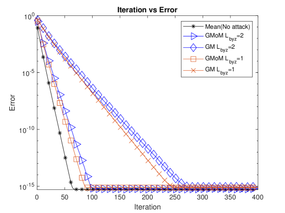
Figure 4: Byz-AltGDmin (Median) vs Byz-AltGDmin (MoM) for $L_{byz}=1,2$; $L=18$

We compare Byz-AltGDmin (Median) with Byz-AltGDmin (MoM) for both values of $L_{byz}$. We also provide results for the baseline algorithm - basic AltGDmin in the no attack setting. All these are compared in Figure 4(b). We also compare the initialization errors in Figure 4(a). As can be seen SubsMoM based initialization error is quite a bit lower than that with SubsMed. The same is true for the GDmin iterations.

VII Discussion

VII-A Novelty of algorithmic and proof techniques

The design and analysis of the Subspace Median algorithm, and obtaining its important corollaries, required novel (yet simple) ideas. We used the fact that the Frobenius norm distance between two subspace projection matrices is within a constant factor of the Frobenius norm subspace distance $\bm{SD}_{F}({\bm{U}}_{1},{\bm{U}}_{2})$. A second key fact is that these projection matrices are bounded by $\sqrt{r}$ in Frobenius norm, We use these facts and Lemma 2.3 (GM lemma for bounded inputs) to prove our key lemma, Lemma 3.8, which is then combined with the Davis-Kahan $\sin\Theta$ theorem to prove Theorem 3.6. This lemma and theorem are likely to be widely applicable in making various other subspace recovery problems Byzantine resilient.

Our analysis of the AltGDmin iterations relies heavily on the lemmas proved in [19] and the overall simplified proof approach developed in [34]. However, we need to modify this approach to deal with the fact that we compute the geometric median of the gradients from the different nodes. The GM analysis provides bounds on Frobenius norms, and hence our analysis also uses the Frobenius norm subspace distance instead of the 2-norm one; see Lemma D.24. At the same time it avoids the complicated proof approach (does not need to use the fundamental theorem of calculus) of [19]. A second new step is the bound on the difference between the expected values of the gradients from two good nodes conditioned on past estimates and data. See Lemma D.26. This lemma is used along with Lemma 2.4 (our GM lemma for potentially unbounded inputs) to obtain Lemma D.27. We expect the overall approach used in this work (use Subspace-Median for initialization and GM of gradients for the GD step) to be useful for making GD-based solutions to various other federated low rank matrix recovery problems Byzantine-resilient. We also expect the Subspace Median algorithm and guarantee to be useful for making various other subspace recovery problems Byzantine resilient.

VII-B Extensions

To our best knowledge, there is no existing provable solution for Byzantine resilient federated PCA or subspace estimation. Thus, the Subspace Median algorithm and its proof techniques are likely to be of independent interest. For example, it should be possible to use a similar approach for the initialization step of vertically federated LRCCS and as well as for that of federated LR matrix completion [35, 36]. In both these cases the node outputs are not i.i.d., but are i.i.d.-like. It can also be used for phase retrieval algorithms’ initialization step, e.g., that of [37].

For some of the above results, we will need to use the generalization described in Remark 4.11. As noted there, our guarantee for the Subspace Median algorithm can be made more general to allow for data vectors $\bm{d}_{k}$ that are zero-mean, sub-Gaussian, and i.i.d.-like instead of i.i.d. In particular, instead of all having covariance $\bm{\Sigma}^{*}$, we can also allow for $\mathbb{E}[\bm{d}_{k}\bm{d}_{k}^{\top}]={\bm{U}}^{*}\bm{S}_{k}{\bm{U}}^{*}{}^{\top}$ with all $\bm{S}_{k}$’s having a large enough singular value gap. The proof will still involve combining Theorem 3.6 with a different application of [31, Theorem 4.7.1] that now bounds the deviation between $\hat{\bm{\Sigma}}_{\ell}=\bm{D}_{\ell}\bm{D}_{\ell}^{\top}/\widetilde{q}$ and $\bar{\bm{\Sigma}^{*}}={\bm{U}}^{*}(\sum_{k}\bm{S}_{k}){\bm{U}}^{*}{}^{\top}/\widetilde{q}$.

For other applications such as (robust) subspace tracking, where the Subspace Median approach may be useful, we may need to combine Theorem 3.6 with a different concentration bound for random matrices. For example, for data vectors $\bm{d}_{k}$ that are bounded, and that have a covariance matrix that is approximately low-rank, one can use [32, Corollary 5.52].

VII-C Open Questions

In the current work, we treated the geometric median computation as a black box. Both for its accuracy and its time complexity, we relied on results from existing work. However, notice that in the Subspace Median algorithm (which is used in all other algorithms in this work), we need a “median" of $r$-dimensional subspaces in $\Re^{n}$. These are represented by their $n\times r$ basis matrices. To find this though, we are computing the geometric median (GM) of vectorized versions of the subspace projection matrices $\mathcal{P}_{\bm{U}}:={\bm{U}}{\bm{U}}^{\top}$ which are of size $n\times n$. Eventually we need to find the subspace whose projection matrix is closest to the GM. An open question is can we develop a more efficient algorithm to do this computation that avoids having to compute the GM of $n^{2}$ length vectors. We will explore the use of power method type ideas for modifying the GM computation algorithm in order to do this. A related question is whether the computation itself be federated to utilize the parallel computation power of the various nodes. In its current form, the entire GM computation is being done at the center.

A second open question is whether we can improve the guarantees for the Subspace Median of Means algorithms by using more sophisticated proof techniques, such as those used in [4]. A third question of interest is how to develop a Byzantine resilient altGDmin-based (or other GD algorithm based) solution for vertically federated LRCCS and for federated LR matrix completion. Both these problems involve non-homogenous gradients and hence will need more assumptions and different approaches.

Attacks	Methods	$T_{pow}=10$
Alternating	SubsMed	0.375(0.348),0.680
	ResPowMeth	1.000(0.972),0.475
Ones	SubsMed	0.369(0.349),0.704
	ResPowMeth	0.999(0.990),0.513
Orthogonal	SubsMed	0.365(0.348),0.689
	ResPowMeth	0.999(0.366),0.500
No Attack	Power(Baseline)	0.187(0.182),0.529

(a)

Attacks	Methods	$T_{pow}=10$	$T_{pow}=1$
Alternating	SubsMed	0.110(0.091),0.689	0.999(0.614),0.326
	ResPowMeth	0.971(0.898),0.497	1.000(0.991),0.049
Ones	SubsMed	0.111(0.091),0.669	0.999(0.607),0.331
	ResPowMeth	0.992(0.952),0.477	0.999(0.990),0.052
Orthogonal	SubsMed	0.106(0.091),0.672	0.999(0.609),0.319
	ResPowMeth	0.223(0.208),0.475	0.999(0.993),0.048
No Attack	Power(Baseline)	0.063(0.050),0.505	0.999(0.605),0.050

(b)

TABLE II: $n=1000$, $L=3$, $L_{byz}=1$, $r=60$, $q=1800$. We report "$\max\bm{SD}_{F}(\text{mean}\bm{SD}_{F}),\text{mean time}$" in each column.

Attacks	Methods	$T_{pow}=10$	$T_{pow}=1$
Alternating	SubsMed	0.062(0.030)	0.997(0.289)
	ResPowMeth	0.177(0.084)	0.999(0.424)
Ones	SubsMed	0.080(0.030)	0.989(0.236)
	ResPowMeth	0.196(0.087)	0.972(0.311)
Orthogonal	SubsMed	0.067(0.033)	0.999(0.228)
	ResPowMeth	0.125(0.066)	0.999(0.375)
No Attack	Power(Baseline)	0.038(0.018)	0.968(0.211)

(a)

Attacks	Methods	$T_{pow}=10$	$T_{pow}=1$
Alternating	SubsMed	0.045(0.020)	0.986(0.227)
	ResPowMeth	0.178(0.080)	0.997(0.336)
Ones	SubsMed	0.048(0.020)	0.999(0.275)
	ResPowMeth	0.157(0.081)	0.999(0.383)
Orthogonal	SubsMed	0.049(0.019)	0.999(0.204)
	ResPowMeth	0.102(0.057)	0.999(0.339)
No Attack	Power	0.033(0.012)	0.975(0.203)

(b)

Attacks	Methods	$T_{pow}=10$	$T_{pow}=1$
Alternating	SubsMed	0.098(0.085)	0.999(0.642)
	ResPowMeth	0.992(0.853)	1.000(0.988)
Ones	SubsMed	0.099(0.084)	0.999(0.625)
	ResPowMeth	0.998(0.905)	0.999(0.989)
Orthogonal	SubsMed	0.103(0.084)	0.999(0.610)
	ResPowMeth	0.223(0.184)	0.999(0.993)
No Attack	Power	0.043(0.036)	0.995(0.604)

(c)

TABLE III: Additional Experiments. We report "$\max\bm{SD}_{F}(\text{mean}\bm{SD}_{F})$" in each column.

Attacks	Methods	$T_{pow}=10$
Alternating	SubsMoM	0.101(0.085)
	SubsMed	0.175(0.150)
	ResPowMeth	0.522(0.463)
Ones	SubsMoM	0.098(0.085)
	SubsMed	0.172(0.150)
	ResPowMeth	0.542(0.502)
Orthogonal	SubsMoM	0.104(0.086)
	SubsMed	0.172(0.151)
	ResPowMeth	0.223(0.191)
No Attack	Power(Baseline)	0.042(0.035)

(a)

Attacks	Methods	$T_{pow}=10$
Alternating	SubsMoM	0.999(0.872)
	SubsMed	0.182(0.152)
	ResPowMeth	0.987(0.894)
Ones	SubsMoM	1.000(1.000)
	SubsMed	0.160(0.147)
	ResPowMeth	0.999(0.948)
Orthogonal	SubsMoM	1.000(1.000)
	SubsMed	0.183(0.151)
	ResPowMeth	0.216(0.179)
No Attack	Power(Baseline)	0.040(0.036)

(b)

TABLE IV: $L=18$, rank-$r+1$ $\bm{\Sigma}^{*}$, $r=60$, $q=3600$, $T_{gm}=10$, $\tilde{L}=6$ for SubsMoM. We report "$\max\bm{SD}_{F}(\text{mean}\bm{SD}_{F})$" in each column.

Method	$L_{byz}=1$	$L_{byz}=2$
SubsMed	0.716(0.665)	0.717(0.667)
SubsMoM	0.477(0.457)	0.475(0.459)

(a)

Appendix A Proofs for Sec III

A-A Proof of Theorem 3.5

Lemma A.17 [28] describes the convergence behavior of power method that is perturbed by a "noise"/perturbation $\bm{G}_{t}$ in each iteration $t$.

Claim A.17.

[Noisy Power Method [28]] Let ${\bm{U}}^{*}$ ($n\times r$) denote top $r$ singular vectors of a symmetric $n\times n$ matrix $\bm{\Phi}^{*}$, and let $\sigma_{i}$ denote it’s $i-$th singular value. Consider the following algorithm (noisy PM).

1. Let ${\bm{U}}_{rand}$ be an $n\times r$ matrix with i.i.d. standard Gaussian entries. Set ${\bm{U}}_{t=0}={\bm{U}}_{rand}$.

2. For $t=1$ to $T_{pow}$ do,

   1. $\hat{\bm{U}}_{t}\leftarrow\bm{\Phi}^{*}{\bm{U}}_{t-1}+\bm{G}_{t}$

   2. $\hat{\bm{U}}_{t}\leftarrow QR(\hat{\bm{U}}_{t})$

If at every step of this algorithm, we have

$$5\|\bm{G}_{t}\|\leq\epsilon_{pow}(\sigma_{r}^{*}-\sigma_{r+1}^{*}),$$

$$5\|{\bm{U}}^{*}{}^{\top}\bm{G}_{t}\|\leq(\sigma_{r}^{*}-\sigma_{r+1}^{*})\frac{\sqrt{r}-\sqrt{r-1}}{\gamma\sqrt{n}}$$

for some fixed parameter $\gamma$ and $\epsilon_{pow}<1/2$. Then w.p. at least $1-\gamma^{-C_{1}}-\exp^{-C_{2}n}$, there exists a $T_{pow}\geq C\frac{\sigma_{r}^{*}}{\sigma_{r}^{*}-\sigma_{r+1}^{*}}\log(\frac{n\gamma}{\epsilon_{pow}})$ so that after $T_{pow}$ steps we have that

$$\|(I-{\bm{U}}_{T_{pow}}{\bm{U}}_{T_{pow}}^{\top}){\bm{U}}^{*}\|\leq\epsilon_{pow}$$

We state below a lower bound on $\sqrt{r}-\sqrt{r-1}$ based on Bernoulli’s inequality.

Fact A.18.

Writing $\sqrt{r}-\sqrt{r-1}=\sqrt{r}\left(1-\sqrt{1-\frac{1}{r}}\right)$ and using Bernoulli’s inequality $(1+r)^{x}\leq 1+xr$ for every real number $0\leq x\leq 1$ and $r\geq-1$ we have $\frac{1}{2\sqrt{r}}<\sqrt{r}-\sqrt{r-1}$

We use Claim A.17 with $\bm{G}_{t}=\bm{\Phi}^{*}{\bm{U}}-GM\{\bm{\Phi}_{\ell}{\bm{U}}\}_{\ell=1}^{L}$ and output ${\bm{U}}_{T_{pow}}\in\Re^{n\times r}$. To apply it, we need $\|\bm{G}_{t}\|$ to satisfy the two bounds given in the claim. We use Lemma 2.4 to bound it.

Suppose that, for at least $\left(1-\tau\right)L$, $\bm{\Phi}_{\ell}$’s,

$$\Pr\{\|\bm{\Phi}_{\ell}-\bm{\Phi}^{*}\| \leq b_{0}\sigma_{1}^{*}{}\}\geq 1-p$$

Since $\|{\bm{U}}\|_{F}=\sqrt{r}$, this implies

$$\Pr\{\|\bm{\Phi}_{\ell}{\bm{U}}-\bm{\Phi}^{*}{\bm{U}}\|_{F}\leq b_{0}\sqrt{r}\sigma_{1}^{*}{}\}\geq 1-p.$$

We use this and apply Lemma 2.4 with $\bm{z}_{\ell}\equiv vec(\bm{\Phi}_{\ell}{\bm{U}})$ and $\tilde{\bm{z}}\equiv vec(\bm{\Phi}^{*}{\bm{U}})$ so that $\|\tilde{\bm{z}}\|=\|\bm{\Phi}^{*}{\bm{U}}\|_{F}\leq\sigma_{1}^{*}{}\sqrt{r}$. Setting $\epsilon_{gm}=b_{0}$ and applying the lemma, we have w.p. at least $1-c_{0}-Lp-\exp\left(-L\psi\left(0.4-\tau,p\right)\right)$

$$\|\bm{G}_{t}\|\leq\|\bm{G}_{t}\|_{F}=\|GM\{\bm{\Phi}_{\ell}{\bm{U}}\}_{\ell=1}^{L}-\bm{\Phi}^{*}{\bm{U}}\|_{F}\leq 14b_{0}\sqrt{r}\sigma_{1}^{*}{}$$

Recall that $\sigma_{r}^{*}-\sigma_{r+1}^{*}\geq\Delta$. We thus need $5\|\bm{G}_{t}\|\leq\epsilon\Delta$ to hold. This will hold with high probability if $b_{0}\sqrt{r}\sigma_{1}^{*}{}\leq\frac{\epsilon\Delta}{70}$. Using Fact A.18 and $\gamma=\sqrt{n}$, for the second condition of Claim A.17 to hold, we need $\|\bm{G}_{t}\|\leq\Delta\frac{1}{10n\sqrt{r}}$. This then implies that we need $b_{0}\sqrt{r}\sigma_{1}^{*}{}\leq\frac{\Delta}{140n\sqrt{r}}$.

Thus we can set $b_{0}=\min\left(\frac{\epsilon}{70\sqrt{r}},\frac{1}{140nr}\right)\frac{\Delta}{\sigma_{1}^{*}{}}$.

We also need $T_{pow}>C\frac{\sigma_{r}^{*}}{\sigma_{r}^{*}-\sigma_{r+1}^{*}}\log(\frac{n\gamma}{\epsilon})$. This holds if we set $T_{pow}=C\frac{\sigma_{r}^{*}}{\Delta}\log(\frac{n\sqrt{n}}{\epsilon})$.

Hence w.p. at least $1-Lp-\exp\left(-L\psi\left(0.4-\tau,p\right)\right)-1/\sqrt{n}-e^{-C_{2}n}\geq 1-Lp-\exp\left(-L\psi\left(0.4-\tau,p\right)\right)-2/\sqrt{n}$

$$\bm{SD}_{F}({\bm{U}}_{out},{\bm{U}}^{*})\leq\epsilon$$

A-B Proof of Theorem 3.6: SVD at nodes computed using power method

Suppose that, for all $\ell\in\mathcal{J}_{good}$,

$$\Pr\{\|\bm{\Phi}_{\ell}-\bm{\Phi}^{*}\| \leq b_{0}\}\geq 1-p$$

Using Claim 3.9, if $b_{0}<(1-1/\sqrt{2})\Delta$, this implies that, for all $\ell\in\mathcal{J}_{good}$, w.p. at least $1-p$,

$$\bm{SD}_{F}({\bm{U}}_{\ell},{\bm{U}}^{*}) \leq\frac{2\sqrt{r}b_{0}}{\Delta}$$ (4)

Suppose that $\hat{\bm{U}}_{\ell}$ is an estimate of ${\bm{U}}_{\ell}$ computed using the power method. Next we use Claim A.17 to help guarantee that $\bm{SD}_{F}(\hat{\bm{U}}_{\ell},{\bm{U}}_{l})$ is also bounded by $2\sqrt{r}b_{0}/\Delta$. Using Claim A.17 with $\bm{\Phi}=\bm{\Phi}_{\ell}$, ${\bm{U}}={\bm{U}}_{\ell}$, $\bm{G}_{\tau}=0$ for all $\tau$, $\epsilon_{pow}=\frac{2b_{0}}{\Delta}$, and $\gamma=n^{10}$, we can conclude that if $T_{pow}>C\frac{\sigma_{r}(\bm{\Phi}_{\ell})}{\sigma_{r}(\bm{\Phi}_{\ell})-\sigma_{r+1}(\bm{\Phi}_{\ell})}\log(\frac{n\cdot n^{10}}{\epsilon_{pow}}),$ then $\bm{SD}_{2}(\hat{\bm{U}}_{\ell},{\bm{U}}_{\ell})\leq\epsilon_{pow}=\frac{2b_{0}}{\Delta}$ w.p. at least $1-p-1/n^{10}$. Here $\sigma_{i}=\sigma_{i}(\bm{\Phi}_{\ell})$. Using $\|\bm{\Phi}_{\ell}-\bm{\Phi}^{*}\|\leq b_{0}$ and Weyl’s inequality, $\sigma_{r}-\sigma_{r+1}\geq\Delta-2b_{0}$ and $\sigma_{r}<\sigma_{r}^{*}+b_{0}$. Thus, if

$$T_{pow}\geq C\frac{\sigma_{r}^{*}+b_{0}}{\Delta-2b_{0}}\log(n\frac{\Delta}{b_{0}})$$

then

$$\bm{SD}_{2}(\hat{\bm{U}}_{\ell},{\bm{U}}_{\ell})\leq\epsilon_{pow}=\frac{2b_{0}}{\Delta}$$

w.p. at least $1-p-1/n^{10}$. This then implies that $\bm{SD}_{F}(\hat{\bm{U}}_{\ell},{\bm{U}}_{\ell})\leq\frac{2b_{0}\sqrt{r}}{\Delta}$.

Combining this bound with the Davis-Kahan bound from (4), we can conclude that, w.p. at least $1-p-1/n^{10}$,

$$\bm{SD}_{F}(\hat{\bm{U}}_{\ell},{\bm{U}}^{*}) \leq 2\frac{2\sqrt{r}b_{0}}{\Delta}=4\sqrt{r}\frac{b_{0}}{\Delta}$$ (5)

Applying Lemma 3.8 with $\delta\equiv 4\sqrt{r}\frac{b_{0}}{\Delta}$, this then implies that, w.p. at least $1-\exp(-L\psi(0.4-\tau,p+1/n^{10}))$,

$$\bm{SD}_{F}({\bm{U}}_{out},{\bm{U}}^{*})\leq 23\cdot 4\sqrt{r}\frac{b_{0}}{\Delta}=92\sqrt{r}\frac{b_{0}}{\Delta}$$ (6)

If we want the RHS of the above to be $\leq\epsilon$, we need

$$b_{0}=\frac{\epsilon}{92\sqrt{r}}\Delta$$

and we need $T_{pow}\geq C\frac{\sigma_{r}^{*}+b_{0}}{\Delta-2b_{0}}\log(n\frac{\Delta}{b_{0}})$ with this choice of $b_{0}$. By substituting for $b_{0}$ in the above expression, and upper bounding to simplify it, we get the following as one valid choice of $T_{pow}$

$$T_{pow}=C(1+6\epsilon)\frac{\sigma_{r}^{*}}{\Delta}\log(n\frac{92\sqrt{r}}{\epsilon})$$

This used $(1+\epsilon)(1-2\epsilon)^{-1}<(1+\epsilon)(1+4\epsilon)<1+6\epsilon$ for $\epsilon<1$. Since we are using $C$ to include all constants, and using $\epsilon<1$, this further simplifies to $T_{pow}=C\frac{\sigma_{r}^{*}}{\Delta}\log(\frac{nr}{\epsilon})$

Appendix B Proofs for PCA section, Sec. IV

B-A Proof of Corollary 4.10

This is a corollary of Theorem 3.6 and [31, Theorem 4.7.1] stated next. It gives a high probability bound on the error between an empirical covariance matrix estimate, $\hat{\bm{\Sigma}}=\bm{D}\bm{D}^{\top}/\widetilde{q}$, with the $\widetilde{q}$ columns of $\bm{D}$ being independent sub-Gaussian random vectors $\bm{d}_{k}$, and the true one, $\bm{\Sigma}^{*}$.

Claim B.19 ([31]).

Suppose that the matrix $\bm{D}$ is as defined in Sec. IV. With probability at least $1-2\exp(-n)$,

$$\|\hat{\bm{\Sigma}}-\bm{\Sigma}^{*}\|\leq CK^{2}\sqrt{\frac{n}{\widetilde{q}}}\|\bm{\Sigma}^{*}\|.$$

Here $K$ is the maximum sub-Gaussian norm of $\bm{\Sigma}^{*}{}^{-1/2}\bm{d}_{k}$ over $k$.

Using Theorem 3.6 with $\bm{\Phi}_{\ell}\equiv\hat{\bm{\Sigma}}_{\ell}=\bm{D}_{\ell}\bm{D}_{\ell}^{\top}/\widetilde{q}$, $\bm{\Phi}^{*}\equiv\bm{\Sigma}^{*}$, in order to guarantee $\bm{SD}({\bm{U}}_{out},{\bm{U}}^{*})\leq\epsilon$ w.h.p., we need

$$\|\hat{\bm{\Sigma}}_{\ell}-\bm{\Sigma}^{*}\|\leq\frac{\epsilon\Delta}{92\sqrt{r}}$$

By Claim B.19,

$$\Pr\{\|\hat{\bm{\Sigma}}_{\ell}-\bm{\Sigma}^{*}\|\leq CK^{2}\sqrt{\frac{n}{\widetilde{q}}}\|\bm{\Sigma}^{*}\|\}\geq 1-2\exp(-n)$$

The above bound will be less than $\frac{\epsilon\Delta}{92\sqrt{r}}$ if $\widetilde{q}\geq\frac{92^{2}CK^{4}nr\|\bm{\Sigma}^{*}\|^{2}}{\Delta^{2}\epsilon^{2}}.$

Appendix C Proof of LRCCS Initialization

C-A Lemmas for proving Corollary 5.13

We first state the lemmas from [19] that are used in the proof and then provide the proof.

Lemma C.20.

Define the set

$$\mathcal{E}:=\left\{\tilde{C}(1-\epsilon_{1})\frac{\|\bm{X}^{*}\|_{F}^{2}}{q}\leq\alpha_{\ell}\leq\tilde{C}(1+\epsilon_{1})\frac{\|\bm{X}^{*}\|_{F}^{2}}{q}\right\}$$

then $\Pr(\alpha\in\mathcal{E})\geq 1-L\exp(-\tilde{c}\widetilde{m}q\epsilon_{1}^{2})$ where $\alpha=\text{Median}\{\alpha_{\ell}\}_{\ell=1}^{L}$

Proof.

Threshold computation: From [19] Fact 3.7 for all $\ell\in\mathcal{J}_{good}$

$$\Pr\{\alpha_{\ell}\in\mathcal{E}\}\geq 1-\exp(-\tilde{c}\widetilde{m}q\epsilon_{1}^{2})$$

Since more than 75% of $\alpha_{\ell}$’s are good and the median is same as the 50th percentile for a set of scalars. This then implies $\text{Median}\{\alpha_{\ell}\}_{\ell=1}^{L}$ will be upper and lower bounded by good $\alpha_{\ell}$’s. Taking union bound over good $\alpha_{\ell}$’s w.p. at least $1-L\exp(-\tilde{c}\widetilde{m}q\epsilon_{1}^{2})=1-p_{\alpha}$

$$\Pr\{\alpha\in\mathcal{E}\}\geq 1-L\exp(-\tilde{c}\widetilde{m}q\epsilon_{1}^{2})$$

∎

Lemma C.21 ([19]).

Define $(\bm{X}_{0})_{\ell}:=\sum_{k}(\bm{A}_{k})_{\ell}{}^{\top}((\bm{y}_{k})_{\ell})_{\mathrm{trunc}}\bm{e}_{k}^{\top},\ \bm{y}_{k,trnc}:=(\bm{y}_{k}\circ\bm{1}_{|\bm{y}_{k}|\leq\sqrt{\alpha}})$. Conditioned on $\alpha$, we have the following conclusions.

1. Let $\zeta$ be a scalar standard Gaussian r.v.. Define,

   $$\beta_{k}(\alpha):=\mathbb{E}[\zeta^{2}\mathbb{1}_{\{\|\bm{x}^{*}_{k}\|^{2}\zeta^{2}\leq\alpha\}}]$$

   Then,

   $$\mathbb{E}[(\bm{X}_{0})_{\ell}|\alpha]=\bm{X}^{*}\bm{D}(\alpha)$$

   where $\bm{D}(\alpha)=diagonal(\beta_{k}(\alpha),k\in[q])$, i.e., $\bm{D}(\alpha)$ is a diagonal matrix of size $q\times q$ with diagonal entries $\beta_{k}$ defined above.

2. Fix $0<\epsilon_{1}<1$. Then w.p. at least $1-\exp[(n+q)-c\epsilon_{1}^{2}\widetilde{m}q/\mu^{2}\kappa^{2}]$

   $$\|(\bm{X}_{0})_{\ell}-\mathbb{E}[(\bm{X}_{0})_{\ell}|\alpha]\|\leq 1.1\epsilon_{1}\|\bm{X}^{*}\|_{F}$$

3. For any $\epsilon_{1}\leq 0.1$, $\min_{k}\mathbb{E}\left[\zeta^{2}\mathbb{1}_{\left\{|\zeta|\leq\tilde{C}\frac{\sqrt{1-\epsilon_{1}}\|\bm{X}^{*}\|_{F}}{\sqrt{q}\|\bm{x}^{*}_{k}\|}\right\}}\right]\geq 0.92$

Fact C.22.

For any $t>0$, $\mathbb{E}[\zeta^{2}\mathbb{1}_{\{\zeta^{2}\leq t\}}]\leq 1$, this then implies $\|\bm{D}(\alpha)\|\leq 1$

C-B Proof of Corollary 5.13

We will apply Theorem 3.6 with $\bm{\Phi}_{\ell}\equiv(\bm{X}_{0})_{\ell}(\bm{X}_{0})_{\ell}^{\top}$, $\bm{\Phi}^{*}\equiv\mathbb{E}[(\bm{X}_{0})_{\ell}|\alpha]\mathbb{E}[(\bm{X}_{0})_{\ell}|\alpha]^{\top}=\bm{X}^{*}\bm{D}(\alpha)^{2}\bm{X}^{*}{}^{\top}$, $\epsilon=\delta_{0}$ and $\Delta=\sigma_{r}(\bm{X}^{*}\bm{D}(\alpha)^{2}\bm{X}^{*}{}^{\top})-\sigma_{r+1}(\bm{X}^{*}\bm{D}(\alpha)^{2}\bm{X}^{*}{}^{\top})$. For this we need to bound $\|(\bm{X}_{0})_{\ell}(\bm{X}_{0})_{\ell}^{\top}-\mathbb{E}[(\bm{X}_{0})_{\ell}|\alpha]\mathbb{E}[(\bm{X}_{0})_{\ell}|\alpha]^{\top}\|$. We can write

$$(\bm{X}_{0})_{\ell}(\bm{X}_{0})_{\ell}^{\top}-\mathbb{E}[(\bm{X}_{0})_{\ell}|\alpha]\mathbb{E}[(\bm{X}_{0})_{\ell}|\alpha]^{\top}$$

$$=(\bm{X}_{0})_{\ell}((\bm{X}_{0})_{\ell}-\mathbb{E}[(\bm{X}_{0})_{\ell}|\alpha])^{\top}$$

$$+((\bm{X}_{0})_{\ell}-\mathbb{E}[(\bm{X}_{0})_{\ell}|\alpha])\mathbb{E}[(\bm{X}_{0})_{\ell}|\alpha]^{\top}$$ (7)

To bound (7) we need the bounds on $(\bm{X}_{0})_{\ell}$, $\mathbb{E}[(\bm{X}_{0})_{\ell}|\alpha]$, and $(\bm{X}_{0})_{\ell}-\mathbb{E}[(\bm{X}_{0})_{\ell}|\alpha]$

1. From Lemma C.21 part 2, letting $\epsilon_{1}=\epsilon_{3}/\sqrt{r}$, w.p. $1-\exp[(n+q)-c\epsilon_{1}^{2}\widetilde{m}q/r\mu^{2}\kappa^{2}]$

   $$\|(\bm{X}_{0})_{\ell}-\mathbb{E}[(\bm{X}_{0})_{\ell}|\alpha]\|\leq 1.1\epsilon_{3}\sigma_{1}^{*}{}$$ (8)

2. From Lemma C.21 part 1, Fact C.22

   $$\|\mathbb{E}[(\bm{X}_{0})_{\ell}|\alpha]\|\leq\sigma_{1}^{*}{}$$ (9)

3. Thus, for $\epsilon_{3}<0.1$, w.p. $1-\exp[(n+q)-c\epsilon_{3}^{2}\widetilde{m}q/r\mu^{2}\kappa^{2}]$

   $$\|(\bm{X}_{0})_{\ell}\| =\|(\bm{X}_{0})_{\ell}-\mathbb{E}[(\bm{X}_{0})_{\ell}|\alpha]\|+\|\mathbb{E}[(\bm{X}_{0})_{\ell}|\alpha]\|$$

   $$\leq 1.1(1+\epsilon_{3})\sigma_{1}^{*}{}<1.3\sigma_{1}^{*}{}$$ (10)

   .

From (7), (8),(9) and (10), and $\mathbb{E}[(\bm{X}_{0})_{\ell}|\alpha]=\bm{X}^{*}\bm{D}(\alpha)$, we have w.p. at least $1-2\exp[(n+q)-c\epsilon_{3}^{2}\widetilde{m}q/r\mu^{2}\kappa^{2}]$

$$\|(\bm{X}_{0})_{\ell}(\bm{X}_{0})_{\ell}^{\top}-\bm{X}^{*}\bm{D}(\alpha)^{2}\bm{X}^{*}{}^{\top}\|\leq$$

$$\|(\bm{X}_{0})_{\ell}\|\|(\bm{X}_{0})_{\ell}-\bm{X}^{*}\bm{D}(\alpha)\|+\|(\bm{X}_{0})_{\ell}-\bm{X}^{*}\bm{D}(\alpha)\|\|\bm{D}(\alpha)\bm{X}^{*}\|$$

$$\leq 1.1.1.1\epsilon_{3}\sigma_{1}^{*}{}^{2}+1.1\epsilon_{3}\sigma_{1}^{*}{}^{2}<2.5\epsilon_{3}\sigma_{1}^{*}{}^{2}$$ (11)

To apply Theorem 3.6 to get $\bm{SD}_{F}({\bm{U}}_{out},{\bm{U}}^{*})<\delta_{0}$, we need $\|(\bm{X}_{0})_{\ell}(\bm{X}_{0})_{\ell}^{\top}-\bm{X}^{*}\bm{D}(\alpha)^{2}\bm{X}^{*}{}^{\top}\|<\frac{\delta_{0}}{26\sqrt{r}}\Delta$. By Lemma C.21 part 3, Fact C.22, and the fact that $\bm{X}^{*}$ is rank $r$ we get a lower bound on $\Delta$

$$\Delta\geq 0.92^{2}\sigma_{r}^{*}{}^{2}-0>0.8\sigma_{r}^{*}{}^{2}$$ (12)

Using (12) and (11), the required condition for Theorem 3.6 holds if

$$2.5\epsilon_{3}\sigma_{1}^{*}{}^{2}\leq 0.8\frac{\delta_{0}}{26\sqrt{r}}\sigma_{r}^{*}{}^{2}$$

This will hold if we set $\epsilon_{3}=\frac{c}{\sqrt{r}\kappa^{2}}\delta_{0}$. With this choice of $\epsilon_{3}$, the bounds hold w.p. at least $1-2\exp[(n+q)-c\delta_{0}^{2}\widetilde{m}q/r^{2}\mu^{2}\kappa^{6}]$

Thus, by Theorem 3.6,

$$\Pr\{SD_{F}({\bm{U}}_{out},{\bm{U}}^{*})\leq\delta_{0}|\alpha\}\geq 1-c_{0}-\exp(-L\psi(0.4-\tau,p+n^{-10}))$$

where $p=2\exp[(n+q)-c\delta_{0}^{2}\widetilde{m}q/r^{2}\mu^{2}\kappa^{6}]$.

Following the same argument as given in proof of [19, Theorem 3.1] and using Lemma C.20 to remove the conditioning on $\alpha$, we get

$$\Pr\{SD_{F}({\bm{U}}_{out},{\bm{U}}^{*})\leq\delta_{0}\}$$

$$\geq 1-c_{0}-\exp(-L\psi(0.4-\tau,p+n^{-10}))-p_{\alpha}$$

where $p_{\alpha}=L\exp(-\tilde{c}\widetilde{m}q\delta_{0}^{2}/r^{2}\kappa^{4})$.

If $\widetilde{m}q\geq C\kappa^{6}\mu^{2}(n+q)r^{2}/\delta_{0}^{2}$, then $p<e^{-c(n+q)}$, and $p_{\alpha}<e^{-c(n+q)}$.

Thus, the good event holds w.p. at least $1-c_{0}-\exp(-L\psi(0.4-\tau,e^{-c(n+q)}+n^{-10}))-e^{-c(n+q)}$.

C-C Proof of Corollary 5.14

In this case, we apply Theorem 3.6 on $\bm{\Phi}_{(\vartheta)}=\sum_{\ell=1}^{\rho}(\bm{X}_{0})_{(\vartheta,\ell)}(\bm{X}_{0})_{(\vartheta,\ell)}^{\top}/(\widetilde{m}\rho)^{2}$ and $\bm{\Phi}^{*}=\mathbb{E}[(\bm{X}_{0})_{\ell}|\alpha]\mathbb{E}[(\bm{X}_{0})_{\ell}|\alpha]^{\top}/\widetilde{m}^{2}$ for $\vartheta\in[\tilde{L}]$. To obtain the bounds needed to apply Theorem 3.6, we use the bounds from above.

Appendix D Proofs for LRCCS AltGDmin iterations

We prove this for the simple GM setting because that is notation-wise simpler. This is the $\tilde{L}=L$ setting. The extension to GMoM is straightforward once again.

All expected values used below are expectations conditioned on past estimates (which are functions of past measurement matrices and measurements, $\bm{A}_{k},\bm{y}_{k}$). For example, $\mathbb{E}[(\nabla_{U}f)_{\ell}]$ conditions on the values of ${\bm{U}},\bm{B}_{\ell}$ used to compute it. This is also the reason why $\mathbb{E}[(\nabla_{U}f)_{\ell}]$ is different for different nodes; see Lemma D.26.

D-A Lemmas for proving Theorem 5.15 for $\tilde{L}=L$: LS step bounds

The next lemma bounds the 2-norm error between $(\bm{b}_{k})_{\ell}$ and an appropriately rotated version of $\bm{b}^{*}_{k}$, $\bm{g}_{k}:={\bm{U}}^{\top}\bm{x}^{*}_{k}=({\bm{U}}^{\top}{\bm{U}}^{*})\bm{b}^{*}_{k}$; followed by also proving various important implications of this bound. Here and below ${\bm{U}}$ denotes the subspace estimate at iteration $t$.

Lemma D.23 (Lemma 3.3 of [19]).

Assume that $\bm{SD}_{F}({\bm{U}},{\bm{U}}^{*})\leq\delta_{t}$. Consider any $\ell\in\mathcal{J}_{good}$. Let $\bm{g}_{k}:={\bm{U}}^{\top}\bm{x}^{*}_{k}=({\bm{U}}^{\top}{\bm{U}}^{*})\bm{b}^{*}_{k}$.

If $\delta_{t}\leq 0.02/\kappa^{2}$, and if $\widetilde{m}\gtrsim\max(\log q,\log n,r)$, for $\epsilon_{1}<0.1$ then,
w.p. at least, $1-\exp(\log q+r-c\epsilon_{1}^{2}\widetilde{m})$

1. $\|(\bm{b}_{k})_{\ell}-\bm{g}_{k}\|\leq 1.7\epsilon_{1}\delta_{t}\|\bm{b}^{*}_{k}\|$

2. $\|(\bm{b}_{k})_{\ell}\|\leq 1.1\|(\bm{b}^{*}_{\ell})_{k}\|$

3. $\|\bm{B}_{\ell}-\bm{G}\|_{F}\leq 1.7\epsilon_{1}\delta_{t}\sigma_{1}^{*}{}$

4. $\|(\bm{x}_{\ell})_{k}-\bm{x}^{*}_{k}\|\leq 1.4\delta_{t}\|\bm{b}^{*}_{k}\|$

5. $\|\bm{X}_{\ell}-\bm{X}^{*}\|_{F}\leq 1.4\delta_{t}\sigma_{1}^{*}{}$

6. $\sigma_{r}(\bm{B}_{\ell})\geq 0.9\sigma_{r}^{*}{}$

7. $\sigma_{\max}(\bm{B}_{\ell})\leq 1.1\sigma_{1}^{*}{}$

(only the last two bounds require the upper bound on $\delta_{t}$).

All the lemmas given below for analyzing the GD step use Lemma D.23 in their proofs.

D-B Lemmas for proving Theorem 5.15 for $\tilde{L}=L$: bounding $\bm{SD}_{F}({\bm{U}}^{+},{\bm{U}}^{*})$

The main goal here is to bound $\bm{SD}_{F}({\bm{U}}^{+},{\bm{U}}^{*})$, given that $\bm{SD}_{F}({\bm{U}},{\bm{U}}^{*})\leq\delta_{t}$. Here ${\bm{U}}^{+}$ is the subspace estimate at the next, $(t+1)$-th iteration. We will show that $\bm{SD}_{F}({\bm{U}}^{+},{\bm{U}}^{*})\leq(1-(\eta\sigma_{1}^{*}{}^{2})\frac{c}{\kappa^{2}})\delta_{t}$. In our previous work [19, 34], we obtained this by bounding the deviation of the gradient, $\nabla f=\sum_{k\in[q]}\nabla f_{k}$ from its expected value, $\mathbb{E}[\nabla f]=m(\bm{X}-\bm{X}^{*})\bm{B}^{\top}$ and then using this simple expression for the expected gradient to obtain the rest of our bounds. In particular notice that $\mathcal{P}_{{\bm{U}}^{*},\perp}\mathbb{E}[\nabla f]=m\mathcal{P}_{{\bm{U}}^{*},\perp}{\bm{U}}\bm{B}\bm{B}^{\top}$.

In this work, to use the same proof structure, we need a proxy for $\mathbb{E}[\nabla f]$. For this, we can use $\mathbb{E}[(\nabla f)_{\ell}]$ for any $\ell\in\mathcal{J}_{good}$. We let $\ell_{1}\in\mathcal{J}_{good}$ be one such node. In what follows, we will use $\mathbb{E}[\nabla f_{\ell_{1}}]=m(\bm{X}_{\ell_{1}}-\bm{X}^{*})\bm{B}_{\ell_{1}}^{\top}$ at various places.

Lemma D.24.

(algebra lemma) Let

$$\mathrm{Err}=\nabla f^{GM}-\mathbb{E}[\nabla f_{\ell_{1}}({\bm{U}},\bm{B})].$$

Recall that ${\bm{U}}^{+}=QR({\bm{U}}-(\eta/\widetilde{m})\nabla f^{GM})$. We have

$$\bm{SD}_{F}({\bm{U}}^{*},{\bm{U}}^{+})\leq\frac{\|\bm{I}_{r}-\eta\bm{B}_{\ell_{1}}\bm{B}_{\ell_{1}}^{\top}\|\bm{SD}_{F}({\bm{U}}^{*},{\bm{U}})+\frac{\eta}{\widetilde{m}}\|\mathrm{Err}\|_{F}}{1-\frac{\eta}{\widetilde{m}}\|\mathbb{E}[\nabla f_{\ell_{1}}({\bm{U}},\bm{B})]\|-\frac{\eta}{\widetilde{m}}\|\mathrm{Err}\|}$$

Proof.

See Appendix D-D. ∎

Lemma D.25.

Assume $\bm{SD}_{F}({\bm{U}}^{*},{\bm{U}})\leq\delta_{t}<\delta_{0}$.

1. If $\eta\leq 0.5/\sigma_{1}^{*}{}^{2}$, $\lambda_{\min}(\bm{I}_{r}-\eta\bm{B}_{\ell_{1}}\bm{B}_{\ell_{1}}^{\top})=1-\eta\|\bm{B}_{\ell_{1}}\|^{2}>1-\eta 1.3\sigma_{1}^{*}{}^{2}>0$ and so this matrix is p.s.d. and hence, $\|\bm{I}_{r}-\eta\bm{B}_{\ell_{1}}\bm{B}_{\ell_{1}}^{\top}\|=\lambda_{\max}(\bm{I}_{r}-\eta\bm{B}_{\ell_{1}}\bm{B}_{\ell_{1}}^{\top})=1-\eta\sigma_{min}(\bm{B}_{\ell_{1}})^{2}\leq 1-\eta 0.8\sigma_{r}^{*}{}^{2}$

2. For all $\ell\in\mathcal{J}_{good}$,

   $$\mathbb{E}[\nabla f_{\ell}({\bm{U}},\bm{B}_{\ell})]=\widetilde{m}(\bm{X}_{\ell}-\bm{X}^{*})\bm{B}_{\ell}^{\top}$$

3. For all $\ell\in\mathcal{J}_{good}$,

   $$\|\mathbb{E}[\nabla f_{\ell}({\bm{U}},\bm{B}_{\ell})]\|_{F}\leq\widetilde{m}1.6\delta_{t}\sigma_{1}^{*}{}^{2}$$

Proof.

The first item follows using the bounds on $\sigma_{1}^{*}{}(\bm{B}_{\ell})$ and $\sigma_{r}^{*}{}(\bm{B}_{\ell})$ from Lemma D.23. Second item is immediate. Third item follows from item two and bounds on $\sigma_{1}^{*}{}(\bm{B}_{\ell})$, $\|\bm{X}_{\ell}-\bm{X}^{*}\|_{F}$ given in Lemma D.23. ∎

Lemma D.26.

Assume $\bm{SD}_{F}({\bm{U}}^{*},{\bm{U}})\leq\delta_{t}<\delta_{0}$. Then, w.p. at least $1-\exp\Big{(}(n+r)-c\epsilon_{1}^{2}\frac{\widetilde{m}q}{r\mu^{2}}\Big{)}-2\exp(\log q+r-c\epsilon_{1}^{2}\widetilde{m})$, for all $\ell\in\mathcal{J}_{good}$,

$$\|\nabla f_{\ell}({\bm{U}},\bm{B}_{\ell})-\mathbb{E}[\nabla f_{\ell_{1}}({\bm{U}},\bm{B}_{\ell_{1}})]\|_{F}\leq\widetilde{m}12.5\sigma_{\max}^{\ast 2}\epsilon_{1}\sqrt{r}\delta_{t}$$

Proof.

Proof is given in Appendix D-E. ∎

The next lemma is an easy consequence of Lemma D.26 and Lemma 2.4.

Lemma D.27.

Let $p_{1}=\exp\Big{(}(n+r)-c\epsilon_{1}^{2}\frac{\widetilde{m}q}{r\mu^{2}}\Big{)}+2\exp(\log q+r-c\epsilon_{1}^{2}\widetilde{m})$. If $\tau<0.4$, then, w.p. at least $1-Lp_{1}-\exp(-L\psi(0.4-\tau,p_{1}))$,

$$\|\mathrm{Err}\|_{F}\leq 14.12.5\widetilde{m}\sigma_{\max}^{\ast 2}\epsilon_{1}\sqrt{r}\delta_{t}$$

Proof.

See Appendix D-F. ∎

D-C Proof of Theorem 5.15

The proof is an easy consequence of the above lemmas. Using the bounds from Lemma D.27, D.25 and the $\bm{SD}_{F}$ bound from Lemma D.24, setting $\epsilon_{1}=0.3/175\sqrt{r}\kappa^{2}$, and using $\delta_{t}\leq\delta_{0}=0.1/\kappa^{2}$ in the denominator terms, we conclude the following: if in each iteration, $\widetilde{m}q\geq C_{1}\kappa^{4}\mu^{2}(n+r)r^{2}$, $\widetilde{m}>C_{2}\max(\log q,\log n)$, then, w.p. at least $1-Lp_{1}-\exp(-L\psi(0.4-\tau,p_{1}))$, where $p_{1}=\exp\Big{(}(n+r)-c\frac{\widetilde{m}q}{r^{2}\kappa^{4}\mu^{2}}\Big{)}+2\exp(\log q+r-c\widetilde{m}/\kappa^{4})$

$$\bm{SD}_{F}({\bm{U}}^{*},{\bm{U}}^{+})\leq\frac{(1-\frac{0.8\eta\sigma_{1}^{*}{}^{2}}{\kappa^{2}})\delta_{t}+\frac{0.3\eta\sigma_{1}^{*}{}^{2}}{\kappa^{2}}\delta_{t}}{1-\frac{1.6\cdot 0.1\eta\sigma_{1}^{*}{}^{2}}{\kappa^{2}}-\frac{0.1\cdot 0.3\eta\sigma_{1}^{*}{}^{2}}{\kappa^{2}}}$$

$\leq(1-(\eta\sigma_{1}^{*}{}^{2})\frac{c}{\kappa^{2}})\delta_{t}:=\delta_{t+1}$ Applying this bound at each $t$ proves the theorem.

The numerical constants may have minor errors in various places.

D-D Proof of Algebra lemma, Lemma D.24

Recall that $\mathrm{Err}=\nabla f^{GM}-\mathbb{E}[\nabla f_{\ell_{1}}({\bm{U}},\bm{B}_{\ell_{1}})]$. Let $\mathcal{P}:=\bm{I}-{\bm{U}}^{*}{\bm{U}}^{*T}$.

GD step is given as $\hat{\bm{U}}^{+}={\bm{U}}-\frac{\eta}{\widetilde{m}}\nabla f^{GM}.$

Adding and subtracting $\mathbb{E}[\nabla f_{\ell_{1}}({\bm{U}},\bm{B}_{\ell_{1}})]=\widetilde{m}(\bm{X}_{\ell_{1}}-\bm{X}^{*})\bm{B}_{\ell_{1}}^{\top}$, we get

$$\hat{\bm{U}}^{+} ={\bm{U}}-\frac{\eta}{\widetilde{m}}\widetilde{m}({\bm{U}}\bm{B}_{\ell_{1}}-\bm{X}^{*})\bm{B}_{\ell_{1}}^{\top}-\frac{\eta}{\widetilde{m}}\mathrm{Err}$$ (13)

Multiplying both sides by $\mathcal{P}:=\bm{I}-{\bm{U}}^{*}{\bm{U}}^{*}{}^{\top}$,

$$\mathcal{P}\hat{\bm{U}}^{+} =\mathcal{P}{\bm{U}}-\eta\mathcal{P}{\bm{U}}\bm{B}_{\ell_{1}}\bm{B}_{\ell_{1}}^{\top}-\frac{\eta}{\widetilde{m}}\mathcal{P}\mathrm{Err}$$

$$=\mathcal{P}{\bm{U}}(\bm{I}_{r}-\eta\bm{B}_{\ell_{1}}\bm{B}_{\ell_{1}}^{\top})-\frac{\eta}{\widetilde{m}}\mathcal{P}\mathrm{Err}$$ (14)

Taking Frobenius norm and using $\|M_{1}M_{2}\|_{F}\leq\|M_{1}\|_{F}\|M_{2}\|$ we get

$$\|\mathcal{P}\hat{\bm{U}}^{+}\|_{F}\leq\|\mathcal{P}{\bm{U}}\|_{F}\|I_{r}-\eta\bm{B}_{\ell_{1}}\bm{B}_{\ell_{1}}^{\top}\|+\frac{\eta}{\widetilde{m}}\|\mathcal{P}\mathrm{Err}\|_{F}$$ (15)

Now $\hat{\bm{U}}^{+}\stackrel{{\scriptstyle QR}}{{=}}{\bm{U}}^{+}R^{+}$ and since $\|M_{1}M_{2}\|_{F}\leq\|M_{1}\|_{F}\|M_{2}\|$, this means that $\bm{SD}({\bm{U}}^{*},{\bm{U}}^{+})\leq\|(I-{\bm{U}}^{*}{\bm{U}}^{*T})\hat{\bm{U}}^{+}\|_{F}\|(R^{+})^{-1}\|$. Since $\|(R^{+})^{-1}\|=1/\sigma_{min}(R^{+})=1/\sigma_{min}(\hat{\bm{U}}^{+})$,

$$\|(R^{+})^{-1}\|=\frac{1}{\sigma_{min}({\bm{U}}-\frac{\eta}{\widetilde{m}}(\mathbb{E}[\nabla f_{\ell_{1}}({\bm{U}},\bm{B}_{\ell_{1}})]+\mathrm{Err}))}$$

$$\leq\frac{1}{1-\frac{\eta}{\widetilde{m}}\|\mathbb{E}[\nabla f_{\ell_{1}}({\bm{U}},\bm{B}_{\ell_{1}})]\|-\frac{\eta}{\widetilde{m}}\|\mathrm{Err}\|}$$

Combining the last two bounds proves our result.

D-E Bounding $\|\nabla f_{\ell}({\bm{U}},\bm{B}_{\ell})-\mathbb{E}[\nabla f_{\ell_{1}}({\bm{U}},\bm{B}_{\ell_{1}})]\|_{F}$: Proof of Lemma D.26

From the proof of [19, Lemma 3.5 item 1 ] we can write w.p. at least $1-\exp\Big{(}(n+r)-c\epsilon_{1}^{2}\frac{\widetilde{m}q}{r\mu^{2}}\Big{)}-2\exp(\log q+r-c\epsilon_{1}^{2}\widetilde{m})$

$$\|\nabla f_{\ell}-\mathbb{E}[\nabla f_{\ell}]\|_{F}\leq 1.5\epsilon_{1}\sqrt{r}\delta_{t}\widetilde{m}\sigma_{\max}^{\ast 2}$$ (16)

Using (16) and Lemma D.25, item 2,

$$\|\nabla f_{\ell}-\mathbb{E}[\nabla f_{\ell_{1}}]\|_{F}\leq$$

$$\|\nabla f_{\ell}-\mathbb{E}[\nabla f_{\ell}]\|_{F}+\|\mathbb{E}[\nabla f_{\ell}]-\mathbb{E}[\nabla f_{\ell_{1}}]\|_{F}\leq$$

$$1.5\epsilon_{1}\sqrt{r}\delta_{t}\widetilde{m}\sigma_{\max}^{\ast 2}$$

$$+\|\widetilde{m}(\bm{X}_{\ell}-\bm{X}^{*})\bm{B}_{\ell}^{\top}-\widetilde{m}(\bm{X}_{\ell_{1}}-\bm{X}^{*})\bm{B}_{\ell_{1}}^{\top}\|_{F}$$ (17)

Using the bounds from Lemma D.23,

$$\|\widetilde{m}(\bm{X}_{\ell}-\bm{X}^{*})\bm{B}_{\ell}^{\top}-\widetilde{m}(\bm{X}_{\ell_{1}}-\bm{X}^{*})\bm{B}_{\ell_{1}}^{\top}\|_{F}$$

$$=\widetilde{m}\|{\bm{U}}(\bm{B}_{\ell}\bm{B}_{\ell}^{\top}-\bm{B}_{\ell_{1}}\bm{B}_{\ell_{1}}^{\top})-\bm{X}^{*}(\bm{B}_{\ell}^{\top}-\bm{B}_{\ell_{1}}^{\top})\|_{F}$$

$$=\widetilde{m}\|{\bm{U}}(\bm{B}_{\ell}\bm{B}_{\ell}^{\top}-\bm{B}_{\ell_{1}}\bm{B}_{\ell_{1}}^{\top}\pm\bm{B}_{\ell}B_{\ell_{1}}^{\top})-\bm{X}^{*}(\bm{B}_{\ell}-\bm{B}_{\ell_{1}})^{\top}\|_{F}$$

$$=\widetilde{m}\|{\bm{U}}\bm{B}_{\ell}(\bm{B}_{\ell}^{\top}-\bm{B}_{\ell_{1}}^{\top})-{\bm{U}}(\bm{B}_{\ell_{1}}-\bm{B}_{\ell})\bm{B}_{\ell_{1}}^{\top}-\bm{X}^{*}(\bm{B}_{\ell}^{\top}-\bm{B}_{\ell_{1}}^{\top})\|_{F}$$

$$\leq\widetilde{m}(1.1\sigma_{1}^{*}{}+1.1\sigma_{1}^{*}{}+\sigma_{1}^{*}{})\|\bm{B}_{\ell}-\bm{B}_{\ell_{1}}\|_{F}$$

$$=\widetilde{m}3.2\sigma_{1}^{*}{}\|\bm{B}_{\ell}-\bm{B}_{\ell_{1}}\pm\bm{G}\|_{F}$$

$$\leq\widetilde{m}3.2\sigma_{1}^{*}{}(\|\bm{B}_{\ell}-\bm{G}\|_{F}+\|\bm{B}_{\ell_{1}}-\bm{G}\|_{F})\leq\widetilde{m}11\sigma_{1}^{*}{}^{2}\epsilon_{1}\sqrt{r}\delta_{t}$$

Using this in (17)

$$\|\nabla f_{\ell}-\mathbb{E}[\nabla f_{\ell_{1}}]\|_{F} \leq 1.5\epsilon_{1}\sqrt{r}\delta_{t}\widetilde{m}\sigma_{1}^{*}{}^{2}+\widetilde{m}11\sigma_{1}^{*}{}^{2}\epsilon_{1}\sqrt{r}\delta_{t}$$

$$\leq\widetilde{m}12.5\sigma_{1}^{*}{}^{2}\epsilon_{1}\sqrt{r}\delta_{t}$$ (18)

w.p. at least $1-\exp\Big{(}(n+r)-c\epsilon_{1}^{2}\frac{\widetilde{m}q}{r\mu^{2}}\Big{)}-2\exp(\log q+r-c\epsilon_{1}^{2}\widetilde{m})$.

D-F Bounding $\mathrm{Err}$: Proof of Lemma D.27

Recall that $Err=\nabla f^{GM}-\mathbb{E}[\nabla f_{\ell_{1}}({\bm{U}},\bm{B}_{\ell_{1}})]$. This bound follows from the Lemma 2.4 and Lemma D.26. We apply Lemma 2.4 with $z_{\ell}\equiv\nabla f_{\ell}$ and $\tilde{z}\equiv\mathbb{E}[\nabla f_{\ell_{1}}({\bm{U}},\bm{B}_{\ell_{1}})]$, $\alpha=0.4$, $\tau<0.4$, $\epsilon\equiv 7.8\epsilon_{1}=\epsilon_{gm}$

To apply the Lemma, we need a high probability bound on

$$\max_{\ell}\|\mathrm{GradErr}_{\ell}\|_{F},\ \mathrm{GradErr}_{\ell}:=\nabla f_{\ell}-\mathbb{E}[\nabla f_{\ell_{1}}({\bm{U}},\bm{B}_{\ell_{1}})]$$

By Lemma D.26, for the $(1-\tau)L$ non-Byzantine nodes,

$$\max_{\ell\in\mathcal{J}_{good}}\|\mathrm{GradErr}_{\ell}\|_{F} \leq\|\nabla f_{\ell}({\bm{U}},\bm{B}_{\ell})-\mathbb{E}[\nabla f_{\ell_{1}}({\bm{U}},\bm{B}_{\ell_{1}})]\|_{F}$$ (19)

$$\leq\widetilde{m}12.5\sigma_{\max}^{\ast 2}\epsilon_{1}\sqrt{r}\delta_{t}$$ (20)

w.p. at least $1-\exp\Big{(}(n+r)-c\epsilon_{1}^{2}\frac{\widetilde{m}q}{r\mu^{2}}\Big{)}-2\exp(\log q+r-c\epsilon_{1}^{2}\widetilde{m}):=1-p_{1}$.

Thus, using Lemma 2.4 w.p. at least $1-Lp_{1}-\exp(-L\psi(0.4-\tau,p_{1}))$,

$$\|\mathrm{Err}\|_{F}\leq 14\widetilde{m}12.5\sigma_{\max}^{\ast 2}\epsilon_{1}\sqrt{r}\delta_{t}$$

Appendix E Geometric Median computation algorithms

The geometric median cannot be computed exactly. We describe below two algorithms to compute it. The first is the approach developed in Cohen et al [24]. This comes with a near-linear computational complexity bound. However, as we briefly explain below this is very complicated to implement and needs too many parameters. No numerical simulation results have been reported using this approach even in [24] itself and not in works that cite it either (to our best knowledge).

The practically used GM approach is Weiszfeld’s algorithm [23], which is a form of iteratively re-weighted least squares algorithms. It is simple to implement and works well in practice. However it either comes with an asymptotic guarantee, or with a finite time guarantee for which the bound on the required number of iterations is not easy to interpret. This bound depends upon the chosen initialization for the algorithm. Because of this, we cannot provide an easily interpretable bound on its computational complexity.

E-A Cohen et al [24]’s algorithm: Nearly Linear Time GM

Algorithm 7 $\mathtt{AccurateMedian}(\epsilon_{GM})$

Input: points $z_{1},...,z_{L}\in\mathbb{R}^{d}$     Input: desired accuracy $\epsilon_{GM}\in(0,1)$

1:  Compute a 2-approximate geometric median and use it to center   Compute $x^{(0)}:=\frac{1}{L}\sum_{i\in[L]}z_{i}$ and $\widetilde{f}_{\ast}:=f(x^{(0)})${Here $f(x)=\sum_{i\in[L]}\|x-z_{i}\|_{2}$}   Let $t_{i}=\frac{1}{400\widetilde{f}_{\ast}}(1+\frac{1}{600})^{i-1}$, $\tilde{\epsilon}_{*}=\frac{1}{3}\epsilon_{GM}$, and $\tilde{t}_{*}=\frac{2L}{\tilde{\epsilon}_{*}\cdot\tilde{f}_{*}}$    Let $\epsilon_{v}=\frac{1}{8}(\frac{\tilde{\epsilon}_{*}}{7L})^{2}$ and let $\epsilon_{c}=(\frac{\epsilon_{v}}{36})^{\frac{3}{2}}$

2:  $x^{(1)}=\mathtt{LineSearch}(x^{(0)},t_{1},t_{1},0,\epsilon_{c})$   Iteratively improve quality of approximation   Let $T_{GM}=\max_{i\in\mathbb{Z}}t_{i}\leq\tilde{t}_{*}$

3:  for $i\in[1,T_{GM}]$ do

3:         Compute $\epsilon_{v}$-approximate minimum eigenvalue and eigenvector of $\nabla^{2}f_{t_{i}}(x^{(i)})$

4:     $(\lambda^{(i)},u^{(i)})=\mathtt{ApproxMinEig}(x^{(i)},t_{i},\epsilon_{v})$

4:         Line search to find $x^{(i+1)}$ such that $\|x^{(i+1)}-x_{t_{i+1}}\|_{2}\leq\frac{\epsilon_{c}}{t_{i+1}}$

5:     $x^{(i+1)}=\mathtt{LineSearch}(x^{(i)},t_{i},t_{i+1},u^{(i)},\epsilon_{c})$

6:  end for

7:  Output: $\epsilon_{GM}$-approximate geometric median $x^{(T_{GM}+1)}$.

The function $\mathtt{ApproxMinEig}$ in Algorithm 7 calculates an approximation of the minimum eigenvector of $\nabla^{2}f_{t}(x)$. This approximation is obtained using the well-known power method, which converges rapidly on matrices with a large eigenvalue gap. By leveraging this property, we can obtain a concise approximation of $\nabla^{2}f_{t}(x)$. The running time of $\mathtt{ApproxMinEig}$ is $\mathcal{O}\left(Ld\log\left(\frac{L}{\epsilon_{GM}}\right)\right)$. This time complexity indicates that the algorithm’s execution time grows linearly with $L$ and $d$ and logarithmically with $L/\epsilon_{GM}$. The function $\mathtt{LineSearch}$ in Algorithm 7 performs a line search on the function $g_{t,y,v}(\alpha)$, as defined in Equation 21. The line search aims to find the minimum value of $g_{t,y,v}(\alpha)$, subject to the constraint $|\mathbf{x}-(\mathbf{y}+\alpha\mathbf{v})|_{2}\leq\frac{1}{49t}$, where $\mathbf{x}$ is the variable being optimized.

$$g_{t,y,v}(\alpha)=\min_{\|x-(y+\alpha v)\|_{2}\leq\frac{1}{49t}}f_{t}(x)$$ (21)

To evaluate $g_{t,y,v}(\alpha)$ approximately, an appropriate centering procedure is utilized. This procedure allows for an efficient estimation of the function’s value. The running time of $\mathtt{LineSearch}$ is $\mathcal{O}\left(Ld\log^{2}\left(\frac{L}{\epsilon_{GM}}\right)\right)$. The time complexity indicates that the algorithm’s execution time grows linearly with $L$ and $d$, while the logarithmic term accounts for the influence of $\frac{L}{\epsilon_{GM}}$ on the running time.

E-B Practical Algorithm: Weiszfeld’s method

Weiszfeld’s algorithm, Algorithm 8, provides a simpler approach for approximating the Geometric Median (GM). It is easier to implement compared to Algorithm 7. It is an iteratively reweighted least squares algorithm. It iteratively refines the estimate by giving higher weights to points that are closer to the current estimate, effectively pulling the estimate towards the dense regions of the point set. The process continues until a desired level of approximation is achieved, often determined by a tolerance parameter, $\epsilon_{GM}$. While the exact number of iterations needed cannot be determined theoretically (as we will see from its guarantees below), the algorithm typically converges reasonably quickly in practice.

We provide here the two known guarantees for this algorithm.

Theorem E.28.

[Corollary 7.1 [23]] Suppose that there is no optimal $\bm{z}\in\mathcal{A}=\{\bm{z}_{1},...,\bm{z}_{L}\}$ such that it minimizes $\sum_{\ell=1}^{L}\left\|\bm{z}-\bm{z}_{\ell}\right\|$. Let $\{z_{t}\}_{t\geq 0}$ be the sequence generated by Weiszfeld’s Algorithm 8 with $z_{0}$ as given in the initialization of Algorithm 8. Then, for any $t\geq 0$, we have $\bm{z}_{t}\notin\mathcal{A}$ and $\bm{z}_{t}\rightarrow\bm{z}^{*}$ as $t\rightarrow\infty$. Here $z^{*}$ is the true GM.

Algorithm 8 Weiszfeld’s Algorithm

Input $\mathcal{A}=\{z_{1},z_{2},...,z_{L}\}$
    Parameters $T$, $\epsilon_{GM}$
    Output $z_{GM}$

  Initialization

  $z_{0}=z_{p}+t_{p}d_{p}$, where

   $p\in\arg\min\{f(z_{i}):1\leq i\leq L\}$, $f(z)=\sum_{i=1}^{L}\left\|z-z_{i}\right\|$ and $d_{p}=\frac{R_{p}}{\|R_{p}\|}$, $t_{p}=\frac{\|R_{p}\|-1}{\mathcal{L}(z_{p})}$

$$\mathcal{L}(z)=\begin{cases}\sum_{i=1}^{L}\frac{1}{\lVert z-z_{i}\rVert}&\quad\text{if}\quad z\notin\mathcal{A}\\ \sum_{i=1,i\neq j}^{L}\frac{1}{\lVert z_{j}-z_{i}\rVert}&\quad\text{if}\quad z=z_{j}\quad(1\leq j\leq L)\\ \end{cases}$$

$$R_{j}=\sum_{i=1,i\neq j}^{L}\frac{z_{j}-z_{i}}{\lVert z_{i}-z_{j}\rVert}$$

  

  Iterative step

  

  $z_{t+1}=\left(\sum_{i=1}^{L}\frac{z_{i}}{\left\lVert z_{i}-z_{t}\right\rVert}\right)\bigg{/}\left(\sum_{i=1}^{L}\frac{1}{\left\lVert z_{i}-z_{t}\right\rVert}\right)$

  

  Terminating Condition

  

  

1. $t>T$ Upper bound on number of iterations

2. $\left\lVert z_{t+1}-z_{t}\right\rVert_{2}<\epsilon_{GM}$

Theorem E.29.

[Theorem 8.2 [23]] Let $\{z_{t}\}_{t\geq 0}$ be the sequence generated by Weiszfeld’s Algorithm 8 with $z_{0}$ as given in the initialization of Algorithm 8. Then, for any $t\geq 0$, we have

$$f(z_{t})-f^{*}\leq\frac{M}{2t}\|z_{0}-z^{*}\|^{2}$$

where $M=\frac{2\mathcal{L}(z_{p})L^{2}}{(\|R_{p}\|-1)^{2}}$. Here $z^{*}$ is the true GM.

The first result above is asymptotic. The second one, Theorem E.29, gives convergence rate of $\mathcal{O}(M/t)$ where $M$ is as defined in the theorem. It is not clear how to upper bound $M$ only in terms of the model parameters ($d,L$ or $z^{*}$). Consequently, the rate of convergence is not clear. Moreover, the expression for $z_{0}$ (initialization) is too complicated and thus it is not clear how to bound $\|z_{0}-z^{*}\|^{2}$. Consequently, one cannot provide an expression for the iteration complexity that depends only on the model parameters.

E-C Proof of Lemma 2.2

$\mathcal{J}_{good}=\{\ell:\|\bm{z}_{\ell}-\tilde{\bm{z}}\|\leq\epsilon\|\tilde{\bm{z}}\|\}$ and define $z^{\ast}:=GM(z_{1},...,z_{L})$ as exact Geometric median.

For $\bm{z}_{\ell}$ with $\ell\in\mathcal{J}_{good}$, we have

$$\|\bm{z}_{{gm}}-\bm{z}_{\ell}\| =\|\bm{z}_{{gm}}-\tilde{\bm{z}}+\tilde{\bm{z}}-\bm{z}_{\ell}\|$$

$$\geq\|\bm{z}_{{gm}}-\tilde{\bm{z}}\|-\|\bm{z}_{\ell}-\tilde{\bm{z}}\|$$

$$\geq\|\bm{z}_{{gm}}-\tilde{\bm{z}}\|-2\epsilon\|\tilde{\bm{z}}\|+\|\bm{z}_{\ell}-\tilde{\bm{z}}\|$$ (22)

Moreover, by triangle inequality for $\bm{z}_{\ell}\notin\mathcal{J}_{good}$, we have

$$\|\bm{z}_{{gm}}-\bm{z}_{\ell}\|\geq\|\bm{z}_{\ell}-\tilde{\bm{z}}\|-\|\bm{z}_{{gm}}-\tilde{\bm{z}}\|$$ (23)

Summing (22), (23) we get

$$\sum_{\ell=1}^{L}\|\bm{z}_{{gm}}-\bm{z}_{\ell}\| \geq\sum_{\ell=1}^{L}\|\bm{z}_{\ell}-\tilde{\bm{z}}\|$$

$$+(2|\mathcal{J}_{good}|-L)\|\bm{z}_{{gm}}-\tilde{\bm{z}}\|-2|\mathcal{J}_{good}|\epsilon\|\tilde{\bm{z}}\|$$

By definition of $\bm{z}_{gm}$ (approximate GM), $\sum_{\ell=1}^{L}\|\bm{z}_{{gm}}-\bm{z}_{\ell}\|\leq(1+\epsilon_{{gm}})\sum_{\ell=1}^{L}\|\bm{z}^{\ast}-\bm{z}_{\ell}\|$. Hence,

$$\sum_{\ell=1}^{L}\|\bm{z}_{\ell}-\tilde{\bm{z}}\|+(2|\mathcal{J}_{good}|-L)\|\bm{z}_{{gm}}-\tilde{\bm{z}}\|-2|\mathcal{J}_{good}|\epsilon\|\tilde{\bm{z}}\|$$

$$\leq(1+\epsilon_{{gm}})\sum_{\ell=1}^{L}\|\bm{z}^{\ast}-\bm{z}_{\ell}\|$$

Since $\bm{z}^{\ast}$ is the minimizer of $\min_{\bm{z}\in\Re^{n}}\sum_{\ell=1}^{L}\|\bm{z}-\bm{z}_{\ell}\|$, so

$$\sum_{\ell=1}^{L}\|\bm{z}^{\ast}-\bm{z}_{\ell}\|\leq\sum_{\ell=1}^{L}\|\bm{z}_{\ell}-\tilde{\bm{z}}\|.$$

Using this to lower bound the first term on the LHS of above,

$$\sum_{\ell=1}^{L}\|\bm{z}^{\ast}-\bm{z}_{\ell}\|+(2|\mathcal{J}_{good}|-L)\|\bm{z}_{{gm}}-\tilde{\bm{z}}\|-2|\mathcal{J}_{good}|\epsilon\|\tilde{\bm{z}}\|$$

$$\leq(1+\epsilon_{{gm}})\sum_{\ell=1}^{L}\|\bm{z}^{\ast}-\bm{z}_{\ell}\|$$

Arranging the terms and using the fact $|\mathcal{J}_{good}|\geq(1-\alpha)L$ we get

$$\|\bm{z}_{{gm}}-\tilde{\bm{z}}\|$$

$$\leq\frac{2|\mathcal{J}_{good}|\epsilon\|\tilde{\bm{z}}\|}{2|\mathcal{J}_{good}|-L}+\epsilon_{{gm}}\frac{\sum_{\ell=1}^{L}\|\bm{z}^{\ast}-\bm{z}_{\ell}\|}{2|\mathcal{J}_{good}|-L}$$

$$\leq\frac{2(1-\alpha)\epsilon\|\tilde{\bm{z}}\|}{1-2\alpha}+\epsilon_{{gm}}\frac{\max_{\ell\in[L]}\|\bm{z}_{\ell}\|}{1-2\alpha}$$

Using Theorem 2.1 with constant probability $1-c_{0}$ Algorithm 7 obtains $(1+\epsilon_{gm})-$approximate geometric median $\bm{z}_{gm}$ in order $T_{gm}=C\log\left(\frac{L}{\epsilon_{gm}}\right)$ implies with probability $1-c_{0}$

$$\|\bm{z}_{gm}-\tilde{\bm{z}}\|\leq C_{\alpha}\epsilon\|\tilde{\bm{z}}\|+\epsilon_{gm}\frac{\sum_{\ell=1}^{L}\|\bm{z}^{*}-\bm{z}_{\ell}\|}{(1-2\alpha)L}$$

$$\leq C_{\alpha}\epsilon\|\tilde{\bm{z}}\|+\epsilon_{gm}\frac{\max_{\ell\in[L]}\|\bm{z}_{\ell}\|}{1-2\alpha}$$

where $C_{\alpha}:=\frac{2(1-\alpha)}{1-2\alpha}$.

E-D Proof of Lemma 2.3

Given

$$\Pr\{\|\bm{z}_{\ell}-\tilde{\bm{z}}\|\leq\epsilon\|\tilde{\bm{z}}\|\}\geq 1-p$$

then

$$\Pr\left\{\sum_{\ell=1}^{L}\mathbb{1}_{\{\|\bm{z}_{\ell}-\tilde{\bm{z}}\|\leq\epsilon\|\tilde{\bm{z}}\|\}}\geq L(1-\alpha)+L_{byz}\right\}$$

$$\geq\Pr\{T\geq L(1-\alpha)+L_{byz}\}$$

where $T\sim\text{Binomial}(L,1-p)$ (First-order stochastic domination)

By Chernoff’s bound for binomial distributions, the following holds:

$$\Pr\{T\geq L(1-\alpha)+L_{byz}\}\geq 1-\exp(-L\psi(\alpha-\tau,p))$$

where $\tau=\frac{L_{byz}}{L}$

This then implies w.p. at least $1-\exp(-L\psi(\alpha-\tau,p))$,

$$\sum_{\ell=1}^{L}\mathbb{1}_{\{\|\bm{z}_{\ell}-\tilde{\bm{z}}\|\leq\epsilon\|\tilde{\bm{z}}\|\}}\geq L(1-\alpha)+L_{byz}\geq L(1-\alpha)$$

where $\alpha\in(\tau,1/2)$. Using Lemma 2.2

$$\|\bm{z}_{{gm}}-\tilde{\bm{z}}\|\leq C_{\alpha}\epsilon\|\tilde{\bm{z}}\|+\epsilon_{{gm}}\frac{\max_{1\leq\ell\leq L}\|\bm{z}_{\ell}\|}{1-2\alpha}$$

w.p. at least $1-c_{0}-\exp(-L\psi(\alpha-\tau,p))$. Fixing $\alpha=0.4$ we get the result.

E-E Proof of Lemma 2.4

$\mathcal{J}_{good}$ denotes the set of good node (nodes whose estimates $\bm{z}_{\ell}$ satisfy $\|\bm{z}_{\ell}-\tilde{\bm{z}}\|\leq\epsilon\|\tilde{\bm{z}}\|$) with the stated probability. First we need to show that, with high probability, none of the entries of $\mathcal{J}_{good}$ are thresholded out. Using given condition $\Pr\{\|\bm{z}_{\ell}-\tilde{\bm{z}}\|\leq\epsilon\|\tilde{\bm{z}}\|\}\geq 1-p$ and union bound, we conclude that, w.p. at least $1-(1-\tau)Lp$, $\max_{\ell\in\mathcal{J}_{good}}\|\bm{z}_{\ell}\|\leq(1+\epsilon)\|\tilde{\bm{z}}\|=\omega$. This means that, with this probability, none of the $\mathcal{J}_{good}$ elements are thresholded out.

For the set $\{\bm{z}_{1},...,\bm{z}_{L}\}\setminus\{\bm{z}_{\ell}:\|\bm{z}_{\ell}\|>(1+\epsilon)\|\tilde{\bm{z}}\|\}$ we apply Lemma 2.3. Since $\left|\{\bm{z}_{1},...,\bm{z}_{L}\}\setminus\{\bm{z}_{\ell}:\|\bm{z}_{\ell}\|>(1+\epsilon)\|\tilde{\bm{z}}\|\}\right|=L^{\prime}\leq L$,

$(1-\tau)L\leq L^{\prime}\leq L$ implies $\tau^{\prime}\leq\tau<0.4$ hence condition of Lemma 2.3 is satisfied using Lemma 2.3 w.p. at least $1-c_{0}-\exp(-L^{\prime}\psi(0.4-\tau^{\prime},p))-(1-\tau)Lp\geq 1-c_{0}-\exp(-L\psi(0.4-\tau,p))-Lp$,

$$\|\bm{z}_{{gm}}-\tilde{\bm{z}}\|\leq 6\epsilon\|\tilde{\bm{z}}\|+5\epsilon_{gm}(1+\epsilon)\|\tilde{\bm{z}}\|<14\max(\epsilon,\epsilon_{gm})\|\tilde{\bm{z}}\|$$

Appendix F One step Analysis of ResPowMeth

If we want to analyze ResPowMeth directly, we need to bound $\bm{SD}(\hat{\bm{U}},{\bm{U}}^{*})$ at each iteration. Consider its first iteration.

Let $\mathcal{P}_{{\bm{U}}^{*},\perp}=\bm{I}-{\bm{U}}^{*}{\bm{U}}^{\ast\top}$, $GM=GM\{\bm{\Phi}_{\ell}{\bm{U}}_{rand}\}_{\ell=1}^{L}$. Then,

$$\bm{SD}_{F}({\bm{U}}^{*},\hat{{\bm{U}}})\leq\|\mathcal{P}_{{\bm{U}}^{*},\perp}GM\|_{F}\|(R^{+})^{-1}\|\leq\frac{\|\mathcal{P}_{{\bm{U}}^{*},\perp}GM\|_{F}}{\sigma_{min}(GM)}$$

Here $GM\stackrel{{\scriptstyle QR}}{{=}}\hat{{\bm{U}}}R^{+}$. This follows since $\|(R^{+})^{-1}\|=1/\sigma_{min}(R^{+})=1/\sigma_{min}(GM)$.

To bound both numerator and denominator, we use the fact that $GM$ is an approximation of $\bm{\Phi}^{*}{\bm{U}}_{rand}$.

Suppose that

$$\|\bm{\Phi}_{\ell}-\bm{\Phi}^{*}\| \leq b_{0}.$$

Using [31, Theorem 4.4.5], $\|{\bm{U}}_{rand}\|\leq 1.1(\sqrt{n}+\sqrt{r})$, and so,

$$\|\bm{\Phi}_{\ell}{\bm{U}}_{rand}-\bm{\Phi}^{*}{\bm{U}}_{rand}\| \leq b_{0}\|{\bm{U}}_{rand}\|\leq 2.2b_{0}\sqrt{n}$$

where we used $r\leq n$. Using this and applying Lemma 2.4 with $\epsilon_{gm}=b_{0}$, we have w.p. at least $1-c_{0}-Lp-\exp\left(-L\psi\left(0.4-\tau,p\right)\right)$

$$\|GM-\bm{\Phi}^{*}{\bm{U}}_{rand}\|\leq 31b_{0}\sqrt{n}$$

Then,

$$\|\mathcal{P}_{{\bm{U}}^{*},\perp}GM\|_{F}$$

$$=\|\mathcal{P}_{{\bm{U}}^{*},\perp}(GM-\bm{\Phi}^{*}{\bm{U}}_{rand}+\bm{\Phi}^{*}{\bm{U}}_{rand})\|_{F}$$

$$=\|\mathcal{P}_{{\bm{U}}^{*},\perp}(GM-\bm{\Phi}^{*}{\bm{U}}_{rand})\|_{F}+\|\mathcal{P}_{{\bm{U}}^{*},\perp}\bm{\Phi}^{*}{\bm{U}}_{rand})\|_{F}$$

$$\leq\|GM-\bm{\Phi}^{*}{\bm{U}}_{rand}\|_{F}+\sigma_{r+1}^{*}\|{\bm{U}}_{rand}\|\sqrt{r}$$

$$=31b_{0}\sqrt{n}+\sigma_{r+1}^{*}\cdot 2.2\sqrt{n}\cdot\sqrt{r}$$ (24)

where we used $\|\mathcal{P}_{{\bm{U}}^{*},\perp}\bm{\Phi}^{*}{\bm{U}}_{rand})\|_{F}\leq\|\mathcal{P}_{{\bm{U}}^{*},\perp}\bm{\Phi}^{*}\|\|{\bm{U}}_{rand})\|_{F}\leq\sigma_{r+1}^{*}\|{\bm{U}}_{rand}\|\sqrt{r}$. Also,

$$\sigma_{min}(GM)$$ (25)

$$\geq\sigma_{min}(\bm{\Phi}^{*}{\bm{U}}_{rand})-\|\bm{\Phi}^{*}{\bm{U}}_{rand}-GM\|$$

$$\geq\sigma_{min}(\bm{\Phi}^{*}{\bm{U}}_{rand})-31b_{0}\sqrt{n}$$

$$\geq\sigma_{min}(\mathcal{P}_{{\bm{U}}^{*}}\bm{\Phi}^{*}{\bm{U}}_{rand})-\|\mathcal{P}_{{\bm{U}}^{*},\perp}\bm{\Phi}^{*}{\bm{U}}_{rand}\|-31b_{0}\sqrt{n}$$

$$\geq\sigma_{min}(\mathcal{P}_{{\bm{U}}^{*}}\bm{\Phi}^{*}{\bm{U}}_{rand})-2.2\sigma_{r+1}^{*}\sqrt{n}-31b_{0}\sqrt{n}$$ (26)

where we used Weyl’s inequality and $\bm{\Phi}^{*}{\bm{U}}_{rand}=\mathcal{P}_{{\bm{U}}^{*}}\bm{\Phi}^{*}{\bm{U}}_{rand}+\mathcal{P}_{{\bm{U}}^{*},\perp}\bm{\Phi}^{*}{\bm{U}}_{rand}$ Finally,

$$\sigma_{min}(\mathcal{P}_{{\bm{U}}^{*}}\bm{\Phi}^{*}{\bm{U}}_{rand}) =\sigma_{min}({\bm{U}}^{*}\bm{\Sigma}{\bm{U}}^{*}{}^{\top}{\bm{U}}_{rand})$$

$$\geq\sigma_{\min}({\bm{U}}^{*})\sigma_{r}^{*}\sigma_{min}\left({\bm{U}}^{*\top}{\bm{U}}_{rand}\right)$$ (27)

We bound $\sigma_{min}\left({\bm{U}}^{*\top}{\bm{U}}_{rand}\right)$ using [38, Theorem 1.1] which helps bound the minimum singular value of square matrices with i.i.d. zero-mean sub-Gaussian entries. $i,j$-th entry of ${\bm{U}}^{*\top}{\bm{U}}_{rand}$ is the inner product of $i$-th column of ${\bm{U}}^{*}$ and $j-$th column of ${\bm{U}}_{rand}$. ${\bm{U}}^{*}$ has orthonormal columns and hence each entry of ${\bm{U}}^{*\top}{\bm{U}}_{rand}$ is mean-zero, unit variance Gaussian r.v. Thus, by [38, Theorem 1.1], w.p., at least $1-(C\epsilon)-\exp^{-cr}$

$$\sigma_{min}({\bm{U}}^{*\top}{\bm{U}}_{rand}) \geq\epsilon(\sqrt{r}-\sqrt{r-1})$$

$$=\epsilon\sqrt{r}\left(1-\sqrt{1-\frac{1}{r}}\right)$$

$$\geq\epsilon\sqrt{r}\left(1-\left(1-\frac{1}{2r}\right)\right)$$

$$=\epsilon\frac{1}{2\sqrt{r}}$$

In the above, we used Bernoulli inequality $(1+x)^{n}\leq 1+nx$, where $0\leq n\leq 1$, $x\geq-1$ for $\sqrt{1-\frac{1}{r}}$. Use $\epsilon=0.1$.

Thus, w.p. at least $1-0.1-\exp^{-cr}$,

$$\sigma_{min}(GM)\geq\sigma_{r}^{*}0.1\frac{1}{2\sqrt{r}}-2.2\sigma_{r+1}^{*}\sqrt{n}-31b_{0}\sqrt{n}$$

Together this implies

$$\bm{SD}_{F}({\bm{U}}^{*},\hat{{\bm{U}}}) \leq\frac{31b_{0}\sqrt{n}+\sigma_{r+1}^{*}\cdot 2.2\sqrt{n}\cdot\sqrt{r}}{\sigma_{r}^{*}0.1\frac{1}{2\sqrt{r}}-2.2\sigma_{r+1}^{*}\sqrt{n}-31b_{0}\sqrt{n}}$$ (28)

$$\leq\frac{62b_{0}\sqrt{nr}+4.4\sigma_{r+1}^{*}\sqrt{n}\cdot r}{\sigma_{r}^{*}0.1-4.4\sigma_{r+1}^{*}\sqrt{nr}-62b_{0}\sqrt{nr}}$$ (29)

To get this bound below $\epsilon_{1}$, we need $b_{0}\leq c\epsilon_{1}/\sqrt{nr}$ and we need $\sigma_{r+1}^{*}<c/(\sqrt{n}r)$. Thus even to get $\epsilon_{1}=0.99$ (any value less than one), we need $b_{0}$ to be of order $1/\sqrt{nr}$.

References

-
[1]
Kairouz, Peter and McMahan, H Brendan and Avent, Brendan and Bellet,
Aur
’elien and Bennis, Mehdi and Bhagoji, Arjun Nitin and Bonawitz, Kallista and Charles, Zachary and Cormode, Graham and Cummings, Rachel and others, “Advances and open problems in federated learning,” Foundations and Trends
textregistered in Machine Learning, vol. 14, no. 1–2, pp. 1–210, 2021. - [2] Chen, Yudong and Su, Lili and Xu, Jiaming, “Distributed statistical machine learning in adversarial settings: Byzantine gradient descent,” Proceedings of the ACM on Measurement and Analysis of Computing Systems, vol. 1, no. 2, pp. 1–25, 2017.
- [3] Blanchard, Peva and El Mhamdi, El Mahdi and Guerraoui, Rachid and Stainer, Julien, “Machine learning with adversaries: Byzantine tolerant gradient descent,” Advances in Neural Information Processing Systems, vol. 30, 2017.
- [4] Yin, Dong and Chen, Yudong and Kannan, Ramchandran and Bartlett, Peter, “Byzantine-robust distributed learning: Towards optimal statistical rates,” in International Conference on Machine Learning. PMLR, 2018, pp. 5650–5659.
- [5] Xie, Cong and Koyejo, Sanmi and Gupta, Indranil, “Zeno: Distributed stochastic gradient descent with suspicion-based fault-tolerance,” in International Conference on Machine Learning. PMLR, 2019, pp. 6893–6901.
- [6] Alistarh, Dan and Allen-Zhu, Zeyuan and Li, Jerry, “Byzantine stochastic gradient descent,” Advances in Neural Information Processing Systems, vol. 31, 2018.
- [7] Cao, Xiaoyu and Fang, Minghong and Liu, Jia and Gong, Neil Zhenqiang, “Fltrust: Byzantine-robust federated learning via trust bootstrapping,” arXiv preprint arXiv:2012.13995, 2020.
- [8] Allen-Zhu, Zeyuan and Ebrahimian, Faeze and Li, Jerry and Alistarh, Dan, “Byzantine-resilient non-convex stochastic gradient descent,” arXiv preprint arXiv:2012.14368, 2020.
- [9] Wu, Zhaoxian and Ling, Qing and Chen, Tianyi and Giannakis, Georgios B, “Federated variance-reduced stochastic gradient descent with robustness to byzantine attacks,” IEEE Transactions on Signal Processing, vol. 68, pp. 4583–4596, 2020.
- [10] Defazio, Aaron and Bach, Francis and Lacoste-Julien, Simon, “SAGA: A fast incremental gradient method with support for non-strongly convex composite objectives,” Advances in neural information processing systems, vol. 27, 2014.
- [11] Acharya, Anish and Hashemi, Abolfazl and Jain, Prateek and Sanghavi, Sujay and Dhillon, Inderjit S and Topcu, Ufuk, “Robust training in high dimensions via block coordinate geometric median descent,” in International Conference on Artificial Intelligence and Statistics. PMLR, 2022, pp. 11145–11168.
- [12] Pillutla, Krishna and Kakade, Sham M and Harchaoui, Zaid, “Robust aggregation for federated learning,” arXiv preprint arXiv:1912.13445, 2019.
- [13] Data, Deepesh and Diggavi, Suhas, “Byzantine-resilient SGD in high dimensions on heterogeneous data,” in 2021 IEEE International Symposium on Information Theory (ISIT). IEEE, 2021, pp. 2310–2315.
- [14] Li, Liping and Xu, Wei and Chen, Tianyi and Giannakis, Georgios B and Ling, Qing, “RSA: Byzantine-robust stochastic aggregation methods for distributed learning from heterogeneous datasets,” in Proceedings of the AAAI Conference on Artificial Intelligence, 2019, vol. 33, pp. 1544–1551.
- [15] Ghosh, Avishek and Hong, Justin and Yin, Dong and Ramchandran, Kannan, “Robust federated learning in a heterogeneous environment,” arXiv preprint arXiv:1906.06629, 2019.
- [16] Regatti, Jayanth and Chen, Hao and Gupta, Abhishek, “Byzantine Resilience With Reputation Scores,” in 2022 58th Annual Allerton Conference on Communication, Control, and Computing (Allerton). IEEE, 2022, pp. 1–8.
- [17] Lu, Shiwei and Li, Ruihu and Chen, Xuan and Ma, Yuena, “Defense against local model poisoning attacks to byzantine-robust federated learning,” Frontiers of Computer Science, vol. 16, no. 6, pp. 166337, 2022.
- [18] Cao, Xinyang and Lai, Lifeng, “Distributed gradient descent algorithm robust to an arbitrary number of byzantine attackers,” IEEE Transactions on Signal Processing, vol. 67, no. 22, pp. 5850–5864, 2019.
- [19] S. Nayer and N. Vaswani, “Fast and sample-efficient federated low rank matrix recovery from column-wise linear and quadratic projections,” Feb. 2023.
- [20] Silpa Babu, Sajan Goud Lingala, and Namrata Vaswani, “Fast low rank compressive sensing for accelerated dynamic mri,” revised and resubmitted, 2022.
- [21] Rakshith Sharma Srinivasa, Kiryung Lee, Marius Junge, and Justin Romberg, “Decentralized sketching of low rank matrices,” 2019, pp. 10101–10110.
- [22] Endre Weiszfeld, “Sur le point pour lequel la somme des distances de n points donnés est minimum,” Tohoku Mathematical Journal, First Series, vol. 43, pp. 355–386, 1937.
- [23] Beck, Amir and Sabach, Shoham, “Weiszfeld’s method: Old and new results,” Journal of Optimization Theory and Applications, vol. 164, no. 1, pp. 1–40, 2015.
- [24] Cohen, Michael B and Lee, Yin Tat and Miller, Gary and Pachocki, Jakub and Sidford, Aaron, “Geometric median in nearly linear time,” in Proceedings of the forty-eighth annual ACM symposium on Theory of Computing, 2016, pp. 9–21.
- [25] Stanislav Minsker, “Geometric median and robust estimation in banach spaces,” 2015.
- [26] Golub, Gene H and Van Loan, Charles F, “Matrix computations,” The Johns Hopkins University Press, Baltimore, USA, 1989.
- [27] Wu, Sissi Xiaoxiao and Wai, Hoi-To and Li, Lin and Scaglione, Anna, “A review of distributed algorithms for principal component analysis,” Proceedings of the IEEE, vol. 106, no. 8, pp. 1321–1340, 2018.
- [28] Hardt, Moritz and Price, Eric, “The noisy power method: A meta algorithm with applications,” Advances in neural information processing systems, vol. 27, 2014.
- [29] Yu, Yi and Wang, Tengyao and Samworth, Richard J, “A useful variant of the Davis–Kahan theorem for statisticians,” Biometrika, vol. 102, no. 2, pp. 315–323, 2015.
-
[30]
Chen, Yuxin and Chi, Yuejie and Fan, Jianqing and Ma, Cong and others,
“Spectral methods for data science: A statistical perspective,”
Foundations and Trends
textregistered in Machine Learning, vol. 14, no. 5, pp. 566–806, 2021. - [31] Vershynin, Roman, High-dimensional probability: An introduction with applications in data science, vol. 47, Cambridge university press, 2018.
- [32] Vershynin, Roman, “Introduction to the non-asymptotic analysis of random matrices,” arXiv preprint arXiv:1011.3027, 2010.
- [33] Rajput, Shashank and Wang, Hongyi and Charles, Zachary and Papailiopoulos, Dimitris, “DETOX: A redundancy-based framework for faster and more robust gradient aggregation,” Advances in Neural Information Processing Systems, vol. 32, 2019.
- [34] N. Vaswani, “A simple proof for efficient federated low rank matrix recovery from column-wise linear projections,” arXiv preprint arXiv:2306.17782, 2023.
- [35] E. J. Candes and B. Recht, “Exact matrix completion via convex optimization,” Found. of Comput. Math, , no. 9, pp. 717–772, 2008.
- [36] P. Netrapalli, P. Jain, and S. Sanghavi, “Low-rank matrix completion using alternating minimization,” 2013.
- [37] Y. Chen and E. Candes, “Solving random quadratic systems of equations is nearly as easy as solving linear systems,” 2015, pp. 739–747.
- [38] Rudelson, Mark and Vershynin, Roman, “Smallest singular value of a random rectangular matrix,” Communications on Pure and Applied Mathematics: A Journal Issued by the Courant Institute of Mathematical Sciences, vol. 62, no. 12, pp. 1707–1739, 2009.