Era Splitting - Invariant Learning for
Decision Trees

Abstract

Real-life machine learning problems exhibit distributional shifts in the data from one time to another or from on place to another. This behavior is beyond the scope of the traditional empirical risk minimization paradigm, which assumes i.i.d. distribution of data over time and across locations. The emerging field of out-of-distribution (OOD) generalization addresses this reality with new theory and algorithms which incorporate environmental, or era-wise information into the algorithms. So far, most research has been focused on linear models and/or neural networks. In this research we develop two new splitting criteria for decision trees, which allow us to apply ideas from OOD generalization research to decision tree models, including random forest and gradient-boosting decision trees. The new splitting criteria use era-wise information associated with each data point to allow tree-based models to find split points that are optimal across all disjoint eras in the data, instead of optimal over the entire data set pooled together, which is the default setting. In this paper we describe the problem setup in the context of financial markets. We describe the new splitting criteria in detail and develop unique experiments to showcase the benefits of these new criteria, which improve metrics in our experiments out-of-sample. The new criteria are incorporated into the a state-of-the-art gradient boosted decision tree model in the Scikit-Learn code base, which is made freely available.

1 Introduction

Gradient boosted regression trees[Fri01] and descendent algorithms such as those implemented via the Light Gradient Boosting Machine[Ke+17], XGBoost[CG16], and Scikit-learn’s HistGradientBoostingRegressor[Ped+11] are considered state of the art for many real-world data science problems characterized by medium data size, tabular format, and/or low signal-to-noise ratio[GOV22].

One such data science problem occurs with predicting future returns in the capital markets. When this problem is framed as a standard supervised learning problem, the target variable is assumed to be a continuous score, representing the expected return (alpha) for a particular stock. The input data is the available information about that stock at that particular time. Each stock’s input data and associated target for each date is represented as one row in a data set. We have one row of data for each stock on each date, which we can use to train and evaluate machine learning (ML) models.

However, supervised learning models in their original form are not aware of the date information presented in the data. One row of input data is associated with one target. Samples are assumed to be drawn I.I.D. from the training and test sets, per the empirical risk minimization ERM principal[Vap91]. While in reality we always draw $N$ samples simultaneously from our data set, where $N$ is the number of stocks in our universe. On any date that we wish to create a portfolio, we need the predictions for all $N$ stocks at the same time. These $N$ data points may not be completely I.I.D. either, as there are measurable positive correlations among stocks in the stock market over any particular time period. Indeed these ideas are the foundation of the capital asset pricing model (CAPM) [FF04] and modern portfolio theory [Mar52], as well as the principles of risk factor models such as the Barra risk factor models[BGM22].

Thus if we look at the stock prediction problem with our standard ML understanding, we are violating many of the assumptions that determined the efficacy of our model predictions. Moreover there is date information that isn’t correctly introduced in our model. In this paper we refer to dates as eras interchangeably.

The discrepancy between the foundations of ML theory and the realities of ML application fits into the contemporary literature in the academic field of out-of-distribution generalization (OOD) research[Liu+23]. In this field of study, we recognize that the ERM principle does not hold true for many, if not all, real-life applications. Thus, we do not assume that the data distribution of our training and test sets are the same. Instead, our framework assumes a certain distributional shift among disjoint data sets, and that our models are designed to account for these shifts. In the literature, this concept is often described in terms of environments. In the context of this research, an environment is an era is a date. Drawing data from different environments is analogous to drawing data from different dates.

Environments are simply subsets of our entire data set. We assume that there is some distributional shift in the data-generating process from one environment to another. The purpose of this is to recognize that there may be spurious signals that work in a single or even a group of environments. It is even shown in [Par+20] that these spurious signals can exist when many environments are pooled together. But these spurious signals change or disappear from one environment to another. These spurious signals usually will present themselves as simpler interpretations of the problem, so a naive model will quickly latch onto them. Think of the cow on grass and camel on sand image recognition problem[NAN20]. During training an image classification task, where we want to predict the label of the animal in an image, cows are always displayed on green grass backgrounds and camel always appear on sandy backgrounds. Naive ML models will simply learn to associate the color green with a cow and the color yellow with a camel. Of course, this is a severe over-simplification of the problem. During evaluation, a cow appearing on a sandy background is classified as a camel, and a camel on a grassy background is classified as a cow. A model which latches onto these spurious signals will perform well in-sample, but have severe flaws when evaluating out-of-sample data.

Fortunately there also exist invariant signals that exist which work in all environments. These signals can often be much more complex than the spurious signals, so naive models are not likely to learn these invariant signals as readily. In the above example, the invariant signal is the cow or camel that is actually present in the image. If an ML model truly understands what a camel or cow looks like, then it will have no problem predicting correctly no matter what the background.

The purpose of this field of research is to design ML procedures which allow models to ignore the spurious and learn the invariant signals in data. In the work of [Arj+20], which is considered foundational in the field, the authors define their problem as a constrained optimization problem and convert it into a loss function that can be used in gradient descent-style training procedures. The loss function combines that tradition ERM risk term, which minimizes the average error over all environments, and an additional penalty on the magnitude of the gradients of the error in each environment. The gradient norm term is used to measure the optimality of the solution in each environment. Considerable theoretical and data analysis is performed around this idea, and the technique is implemented via neural networks and shows that it works on synthetic data problems designed for this purpose, such as the Colored MNIST problem.

A similarly influential work[Par+20] also analyzes the phenomenon of spurious and invariant signals existing simultaneously in data, and how to disentangle the signals. Here, the authors look at the loss surface, and describe the co-existence of local minima on the surface where some minima correspond to spurious predictors and others correspond to the invariant predictors that we are searching for. The insight here is to realize that spurious minima occur is some environments and not others, but invariant minima occur in all environments in the same location. We then extend this reasoning to the directions of the gradients of the loss function with respect to the model parameters. The directions of the gradients for invariant minima should agree across all environments but the directions for spurious signals will disagree between environments. In order to realize this understanding practically, there is an alteration made to the traditional gradient descent algorithm which is called the AND-mask. Before propagating the model weights down the gradients at each iteration, first the gradients are computed using data from each environment separately. We check where the directions of the gradients agree over all the environments, and we only propagate the gradients along the dimensions that agree, and not along those that disagree. There is also a variable to adjust the level of agreement we require. With this technique the authors show how neural network models can effectively extract invariant predictors from data why ignoring spurious ones.

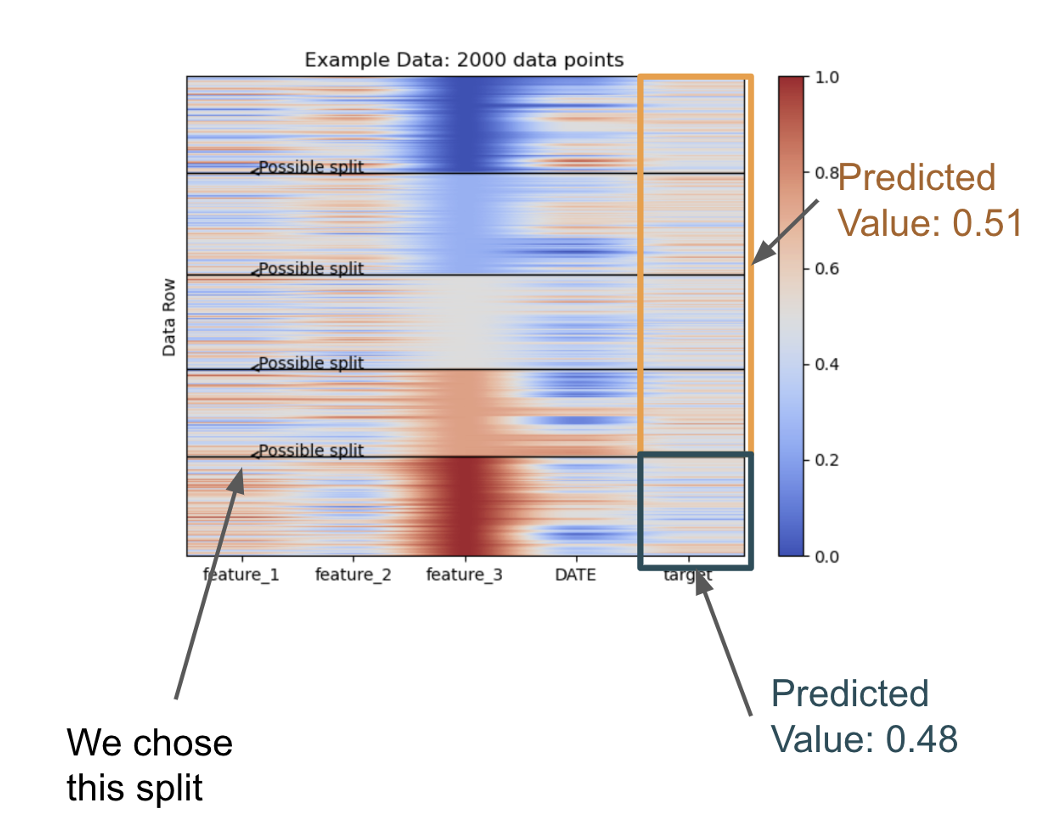
Figure 1: A visual example of a data split point. Here we have a data set of 2,000 data points coming from 8 eras (or environments). All data values are color codes from lowest (blue) to highest (red). Here we visualize a split point that is based on the values of feature 3. We can see we’ve sorted the data by feature 3, and have pointed out the split value. All data points with feature 3 above this value are part of the right child node, and all points below this value are part of the left child node. The value of the right and left child nodes are then computed as the mean value of the targets, in the grey and orange boxes respectively.

Now we introduce what this current paper is proposing. Fitting into the OOD generalization literature, we consider data points coming from distinct environments or eras which have certain distributional shifts in the data generation process. We work in the context of gradient boosted decision trees (GBDT), and related decision tree algorithms. During the course of tree growth, GBDT algorithms partition data in a cascading, step-wise manner by creating split points in the training data[Bre01]. Each split point is defined by a single feature and a single value of that feature data. We start in the root node, which contains all the training data. After finding the optimal split point, all the data with that feature greater than or equal to the split value get partitioned into the left child node, and all other data points go to the right child node child node. We have now grown a tree with depth of 1. In successive steps the child nodes become parent nodes, and the data in those nodes is split in the same manner as the root node. So the question is, how do we choose the optimal split point at each tree node?

The answer to this question is: the splitting criterion. The splitting criterion is a score that is assigned to each possible split of the data at a tree node. We chose the split which has the highest score, as this is the optimal split. Generally speaking, the splitting criterion in GBDTs measures the reduction in impurity from the parent to the child nodes, meaning we chose the split which results in the most pure child nodes. Impurity is measured in the targets, or labels. In binary classification, we thus prefer to split our data using split points that result in child nodes with either just $0$ labels or just $1$ labels. For our task we implement regression, variance as the measure of impurity, so we aim to find splits that result in the greatest reduction in variance from the parent to the child nodes. Here, we present the generally accepted definition of the splitting criterion[CG16].

$$\mathcal{L}_{\text{split}}=\frac{1}{2}\left[\frac{\left(\sum_{i\in I_{L}}g_{i}\right)^{2}}{\sum_{i\in I_{L}}h_{i}+\lambda}+\frac{\left(\sum_{i\in I_{R}}g_{i}\right)^{2}}{\sum_{i\in I_{R}}h_{i}+\lambda}-\frac{\left(\sum_{i\in I}g_{i}\right)^{2}}{\sum_{i\in I}h_{i}+\lambda}\right]$$ (1)

In the above equation, $I$, $I_{L}$, and $I_{R}$ are data set identifiers corresponding to the data of the parent node, the left child node, and the right child node respectively. The $g_{i}$ is the target label (in pure decision trees) corresponding to the $i^{th}$ data point. In GBDTs these are gradients of the loss w.r.t. the predictions of the previous model, so they are labeled $g_{i}$, for $i\in I,I_{L},I_{R}$. The $h_{i}$ are the Hessians. For GBDTs, implementing regression with the mean-squared error loss, the Hessians are constant and equal to 1. The denominators of the three terms above are thus just the counts of the data points in each node. The first term measures the average variance of the left child node $I_{L}$, the second term measures that of the right child node $I_{R}$, and the final term, which has a negative sign, is the average variance of the parent node. This split criterion will have the highest score for a split which results in the lowest average variance in the child nodes, leading to the greatest reduction in average variance from the parent to the children.

In the basic setting, GBDTs pool all the training data together when computing the split criterion. If our training data inherently comes from separate environments (eras), as defined in the OOD literature, what are we losing by pooling all our training data together to find the best split? Would it be better to find splits that treat data from each environment (era) separately? In order to answer this question, we have developed a new splitting criterion, which we call Era Splitting. This new criterion combines the reduction in variance calculation from each era separately into one final new criterion, which is a smooth average of the variance reduction of the era-wise splits. It captures the essence of invariance from the IRM paradigm applied to tree splitting criteria. This method, called era splitting, is introduced in the following section. An additional era-wise splitting criterion is developed in section 3, which is designed after the AND-mask, and looks for splits which maximize the agreement in the direction of the predictions implied by the split for each era (environment). Section 4 then describes our experimental designs, where we develop a toy models aimed at verifying the objectives of our new splitting criteria, and a real-world empirical study, based on the financial stock market, using free data from the Numerai data science tournament. In Section 5 we present results from the experiments and finally in section 6 we provide interpretation of results and discussion about future work.

2 Era Splitting

In order to be concise with definitions, from here on we generally use the term era in the same sense as the term environment is used in the references [Arj+20, Par+20]. An era of data is a disjoint set by which our training and test data sets are comprised of many eras of data. The general understanding is that each era contains data that occurs at certain distinct times and/or physical locations. In the context of the splitting criterion (1), we need to refine the data set definitions $I$, $I_{L}$, and $I_{R}$. With era splitting, we assume that each training data point comes from one of $M$ distinct eras. Thus there exists data sets $I^{j}$, $I_{L}^{j}$, and $I_{R}^{j}$, referring to data coming from the $j^{th}$ era, such that $I^{j}\in I$, $I_{L}^{j}\in I_{l}$, and $I_{R}^{j}\in I_{R}$ for $j\in\{1,2,...,M\}$. Using this convention, we define a new era-wise splitting criterion, which computes the information gain of a split for the $j^{th}$ era.

$$\mathcal{L}_{\text{split}}^{j}=\frac{1}{2}\left[\frac{\left(\sum_{i\in I_{L}^{j}}g_{i}\right)^{2}}{\sum_{i\in I_{L}^{j}}h_{i}+\lambda}+\frac{\left(\sum_{i\in I_{R}^{j}}g_{i}\right)^{2}}{\sum_{i\in I_{R}^{j}}h_{i}+\lambda}-\frac{\left(\sum_{i\in I^{j}}g_{i}\right)^{2}}{\sum_{i\in I^{j}}h_{i}+\lambda}\right]$$ (2)

The era splitting criterion in its basic form is written as a mean average of the era-wise splitting criterion for each era of data.

$$\mathcal{L}_{\text{era split}}=\frac{1}{M}\sum_{j=1}^{M}\mathcal{L}_{\text{split}}^{j}$$ (3)

The era splitting criterion will have the highest score for the split which provides the greatest average increase in information gain over all of the eras. With this criterion we will be less-likely to favor splits which work really well in some eras but not in others. A further generalization we’ve made is by way of a smooth max function, called the Boltzmann operator[AL17]. The Boltzmann operator is an operator that operates on an array of real numbers, and has one parameter, called $\alpha$. When $\alpha=0$, the Boltzmann operator recovers the arithmetic mean, when $\alpha=-\infty$ it recovers the $\min$, and when $\alpha=\infty$ it recovers the $\max$. To define the Boltzmann operator ($\mathcal{B}_{\alpha}$), we consider $n$ real numbers, $x_{i}$ for $i\in\{1,...,n\}$.

$$\mathcal{B}_{\alpha}(x_{1},...,x_{n})=\frac{\sum_{i=1}^{n}x_{i}\exp{(\alpha x_{i})}}{\sum_{i=1}^{n}\exp{(\alpha x_{i})}}$$ (4)

With this generalization we define the final version of the era splitting criterion in equation 5, which is understood as the smooth maximum (minimum) of the era-wise information gains over all of the eras.

$$\mathcal{L}_{\text{era split}}^{\alpha}=\mathcal{B}_{\alpha}\left(\mathcal{L}_{\text{split}}^{1},...,\mathcal{L}_{\text{split}}^{M}\right)$$ (5)

The default value of $\alpha$ is set to zero, which recovers equation 3. Conceptually, varying $\alpha$ toward $-\infty$ will lead us to prefer splits which increase the minimum information gain over all of the eras. This means that we prefer splits that work well in all eras. Conversely, varying $\alpha$ toward positive $\infty$ will cause our algorithm to focus more on splits that improve the best single-era performance, or the maximum information gain over all the era-wise split criteria. In the prior case we prefer splits that have a more uniform affect on information gain over all the eras. In the later case we prefer splits that improve our best performance in any era. In the context of learning an invariant predictor, we would prefer using negative values for $\alpha$.

3 Directional Era Splitting

There is a subtle ambiguity that arises with equation 5, which requires the introduction of the concept of the direction implied by a split. Loosely speaking, a split implies a direction via the values of the child nodes. If the value of the left child node is larger than the value of the right child node, then we can say the direction of this split is too the left. If the value of the right child node is larger, then the direction is to the right. Let the value of the left child node be $v_{l}$, and the value of the right child node be $v_{r}$, then without loss of generality, the direction of split, $d_{\text{split}}$, is defined as the sign of the difference between the left child node value and the right child node value.

$$d_{\text{split}}=\text{sign}(v_{l}-v_{r})$$ (6)

In the traditional setting where we pool all the training data together, we find a split, and there is can only one be direction implied over the entire data set. The traditional splitting criterion does not even consider the direction of the split, since it is superfluous. It doesn’t matter whether the direction implied by the split is to the left or to the right, just as long as the variance of the child nodes is the lowest it can be.

In era splitting, we compute the information gain over each era of data separately, and then summarizing these numbers with a summary statistic (the Boltzmann operator). A problem that arises here is that there could be splits that imply conflicting directions from one era to the next. We can describe the direction of a split in era $j$ by adapting equation 6 with era-wise descriptors, as follows.

$$d_{\text{era split}}^{j}=\text{sign}(v_{l}^{j}-v_{r}^{j})$$ (7)

For each split, we compute the direction implied by this split for each era, resulting in an array of length $M$, $\{d_{\text{era split}}^{0},d_{\text{era split}}^{1},...,d_{\text{era split}}^{M}\}$. With directional era splitting, we require that there is as much agreement in the direction of the split across all of the eras of data. To this end we introduce here the directional era splitting criterion, $\mathcal{D}_{\text{era split}}$, which is a measure of the agreement in the directions of the splits over all of the eras.

$$\mathcal{D}_{\text{era split}}=\frac{1}{M}\left|\sum_{j=0}^{M}d_{\text{era split}}^{j}\right|$$ (8)

Each $d_{\text{era split}}^{j}$ will take a value of either $1$ or $-1$, depending on the direction of the split for that era. So the sum here will be bounded on the interval $[-M,M]$. By taking the absolute value and dividing my $M$, $\mathcal{D}_{\text{era split}}$ is then bounded on the interval $[0,1]$. At the low end, with a value of $0$, half of the directions go in one way while half go in the other way. At the high end, with a value of $1$, all the directions go in the same way. When choosing the best split during tree growth, we choose the highest value for $\mathcal{D}_{\text{era split}}$.

4 Experimental Methods

We’ve designed three experiments to empirically showcase the effects of these new splitting criteria. The first experiment is a toy model which is a simple one-dimensional problem which employs a distributional shift from one era to the next, while also using an invariant signal that stays the same from one era to the next. We call this experiment the shifted sine wave. Secondly we use the synthetic memorization data set present is [Par+20], with a subtle adaptation to a regression objective. Thirdly, we apply these new splitting criteria to simple version of the Numerai tournament data set. The three data sets and experimental setups are described in the following subsections.

4.1 The Shifted Sine Wave Data Set

While there have been other toy model examples in the OOD literature, such as the colored MNIST data set[Arj+20] or the synthetic memorization data set of [Par+20]. These are both classification problems, and we are particularly interested in regression problems. For our purpose we develop a simple 1-dimensional toy model which has an invariant signal which is obscured by two types of randomness. One is a consistent Gaussian blur and the other is a random shift which is consistent inside each era but different across different eras of data. This part in particular simulates the distributional shift in the data generation process from one era to another. Here we remember that an era is equivalent in essence to an environment as proposed in the previous literature.

In order to generate the shifted sine wave data set, we start by defining the number of eras (environments) that we wish to create and the number of data points per era. In any case, the 1-dimensional input data is a random number on the interval $[0,2\pi]$. The dependent, or target, variable is a function of the the input. The invariant part of the target is a sine wave plus standard Gaussian noise. Then, the environmental distribution shift is realized through a vertical shift of the target, where the magnitude of the shift is random, but consistent throughout each era. In this way, each era of data is a blurry sine wave that is shifted by a random amount. After pooling many eras of data together into one data set, we develop a cloud of data where the invariant mechanism, the sine wave, fades away and is not very apparent.

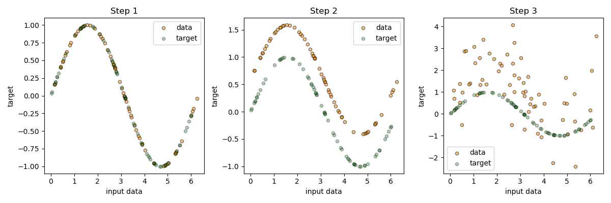
Figure 2: This figure gives a visual description of the data generation process for the shifted sine wave data set. Here we show how one era of data is created. The underlying invariant mechanism (the sine wave) is plotted in green for reference. Step 1 simply applies the sine wave. Step 2 shifts the data by a random amount vertically, and the Step 3 applied the Gaussian noise.

Once we have created our data set, which consists of 64 eras of data, each era having 32 data points, the experiment is simple and straight-forward. We’ve applied the era splitting criterion to Scikit-learn’s decision tree regressor (DecisionTreeRegressor), gradient boosting decision tree regressor (GradientBoostingRegressor), and the histogram gradient boosting decision tree regressor (HistGBR) methods[Ped+11]. The latest is modeled after the state-of-the-art LGBM model[Ke+17], and performance is very comparable between the two models once the parameters have been matched. For this reason, we take the LGBM Regressor model as our baseline model. We then use our implementations of era splitting and directional era splitting implemented in the HistGBR framework as the experimental models.

For each experiment we generate random training (in-sample) and test (out-of-sample) data, each consisting of the same number of eras and data points per era (64 and 32). We then train a baseline LGBM model on the training data and evaluate the performance on the test data. We perform the same procedure for the experimental HistGBR models, which implement the era splitting and directional era splitting criteria in place of the original splitting criterion. The basic parameters used in the experiments are setting the number of boosting rounds (number of trees) to 100, the maximum tree depth to 10 and the learning rate to 1. With this learning rate (also known as the shrinkage rate), the contribution of each tree to the final predictor is large, so the model can fit the data quickly. Setting the maximum depth to 10 creates trees that can be very precise by themselves. This leads to models which have a high in-sample performance and allows us to accentuate the utility of era splitting.

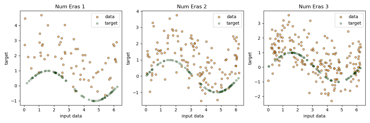
Figure 3: This figure gives another visual description of the data generation process for the shifted sine wave data set. Here we show the process of pooling additional eras to the data in order to create a complete set of data.

In order to evaluate performance, we compute the mean squared error and Pearson correlation of the predictions on the out-of-sample targets, which are generated randomly. We also compute the evaluation metrics using the invariant signal (the sine wave) as the test target, thereby measuring how close our predictions are to the invariant signal. We also include some plots of the predictions as a function of the input variable, to visualize the decision surface. This helps explain the benefit of era splitting visually.

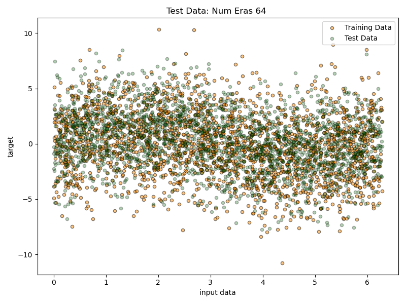
(a) Test Data

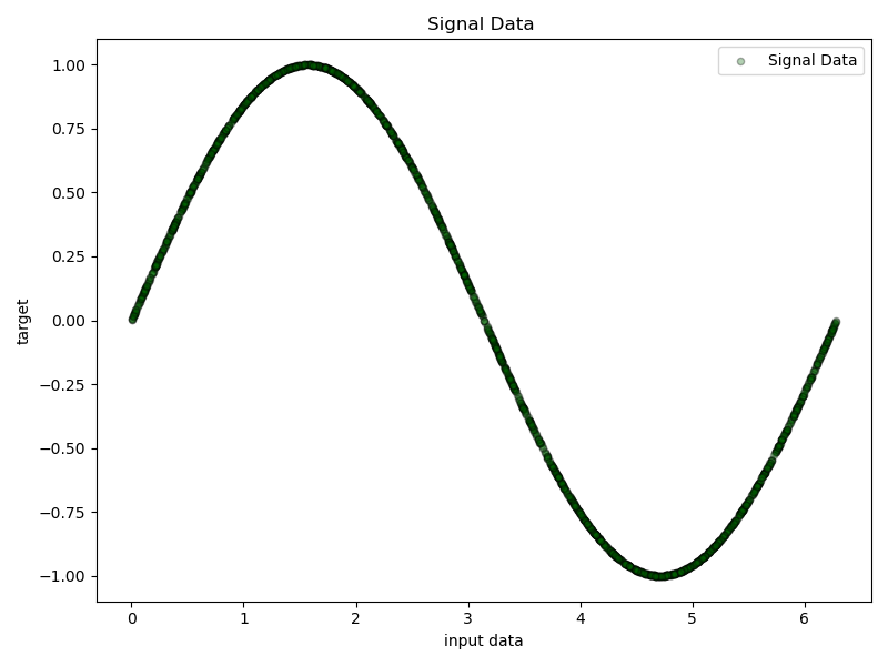
(b) Signal

Figure 4: We provide this figure to help understand the difference between the two evaluation data sets that used in the experiment. The labels on these plots, ”Test Data” and ”Signal” correspond to the labels used in the tables of figure 6.

4.2 Synthetic Memorization Data Set

The synthetic memorization data set was developed in [Par+20] specifically to investigate an ML model’s ability to learn invariant predictors in data even in the presence of simple spurious signals. It is a supervised binary classification task with target labels taking the values $\{0,1\}$. The data set is composed such that the first two input dimensions encode the invariant signal, which is an interlaced spiral shape, where one of the arms belongs to one class, and the other arm the other class. The rest of the input dimensions are used to encode simple shortcuts, or spurious easy-to-learn signals. These are simply two clusters of data points in high dimensions, where one cluster belongs to one class and the other the other class. The clusters are linearly separable, being easy to learn. The spurious aspect is realized through the mechanism that each era (environment) of data has a shift in the location of the two clusters. The shift happens in such a way that, when we pool all the environments of the training data set, the shortcut is still present even though each era of data is slightly different. Refer to figure 5 or Figure 5 from [Par+20] for a visualization of the data in four dimensions. We can see that when we pool environments 1 & 2 together, there is still an easily identifiable linearly separation between the red and the blue dots in the dimensions of the spurious signal.

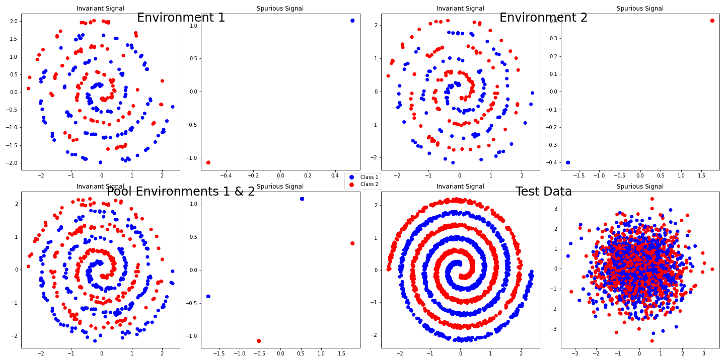
Figure 5: Here we demonstrate how the synthetic memorization data set from [Par+20] is created. In each quadrant of the figure there are two plots. The left plot shows the data in the first two dimensions (the invariant signal), and the right plot shows the data in the second two dimensions (the spurious signal). For the purpose of this figure we restrict the data set to four dimensions. During the larger experiment, the number of dimensions of the spurious signal can be larger, such as 16. The quadrants are labeled. The top left shows the data from environment 1, and the top right from environment 2. The bottom left shows those two environments pooled together, an example of the entire training data. The bottom right then shows the data in the test set. The invariant signal is unchanged while the spurious signal is pure noise.

The big change happens in the test set, where we remove the spurious signal and replace it with noise. Meanwhile we keep the invariant swirl unchanged. Any model that bases its predictions solely on the spurious signal will be worthless when evaluated on the test data. If a model has actually learned the invariant, albeit harder-to-learn signal, it will still perform well on the test set.

This data set was developed specifically to show that most ML models will latch onto the easy spurious signal and completely ignore, or make no attempt to learn the invariant signal. What has been incorporated into this data are disjoint environments, where the relative distribution of the input data is shifting from one era to another. We wish to develop models that, when provided with simply the era-wise (environmental) label for each data point, are able to ignore the shifting spurious signal and learn the invariant signal.

Indeed the authors in [Par+20] developed a technique called the AND-mask, which is an alteration to the naive gradient descent algorithm, incorporating the era-wise information. They were able to show that a naive MLP model simply learns the spurious signals in the data, and performs poorly on the test data. Meanwhile their AND-mask model was able to learn in such a way where it still performs well (98% accuracy) on the test data.

Later in the result, we show a similar result, where a naive gradient boosted tree model learns the spurious signals, and performance is bad on the test set. While our model with directional era splitting is able to learn the invariant signal and perform perfectly on the test set. Indeed, directional era splitting was inspired by the AND-mask, so confirming it works on this data set is paramount.

In order to use a regression model as a classifier, we simply train the model on the classification labels $[0,1]$ and then prediction accordingly. One measure is to take the correlation of the prediction with the class label targets. Besides this measure, we also round the predicted values to either $0$ or $1$, which ever is closer, then we can take traditional classification metrics.

4.3 Numerai Data

Numerai is a San Francisco-based hedge fund which operates via a daily data science tournament in which the company distributes free, obfuscated data to participants, and those participants provide predictions back to Numerai. The predictions represent expected alpha, which is simply a directional up/down, bull/bear style prediction. On any day, a tournament participant will need to produce predictions for 5,000 to 10,000 unique stocks, worldwide. As time goes by, the predictions are then scored against the true realizations that transpire in the markets. These true realizations are called targets.

Numerai distributes a large data set designed for supervised learning. Each row of data represents one stock at one time (era). The rows consists of many input feature columns, and also several target (output) columns. For our purpose we will focus on using the main target, which is also known using the moniker Cyrus. The Cyrus target values correspond to the optimal expected result, which is roughly equivalent to the stock’s future returns in the market subject to company-level risk requirements.

The time periods (eras) are numbered sequentially, starting at 1, and occur at weekly intervals. Each era represents one week of time. Currently there are over 1,060 eras of historical input and target pairs in the data set, and new eras are added each week, as the data becomes available. Each era contains more than 5,000 rows of data, on average, so the entire data set consists of over 5 million rows. The time frame of the targets spans 4 weeks. This is to say, when we enter a prediction, we are scored on the performance of our prediction over the subsequent 4 weeks of time. Currently the full data set provides over 1,600 input features, while also providing medium and small sized feature sets for convenience. For our experiment we chose to use the entire dataset, with all the features and eras available at the time of writing.

The data set is organized into the training set (eras 1 through 578), and the validation set (eras 579 through 1060). The key metric for scoring predictions against the targets is called era-wise correlation, which is simply the Pearson correlation of the predictions with the targets, computed disjointedly on each era of data. These era-wise correlations are the main subject of analysis when comparing one set of predictions with another. The best models will provide predictions with consistently positive era-wise correlation with the target over all the eras. This is indeed the main difficulty with this machine learning problem. Even the best models perform poorly in some eras out-of-sample, even if it is only less than 10% of the eras. These periods of poor performance, also called burn periods, can lead to significant draw downs in hedge fund performance.

For all experiments we kept the parameters of the model fixed across both baseline and experimental setups to a standard set that has proven to work well in practice [Com23]. The parameters are maximum depth of 5, the number of trees is 5,000, and the learning rate is 0.01. We allow the trees to grow to a maximum size only limited by the maximum depth. Furthermore we’ve implemented the colsample-bytree method from LightGBM, which builds each tree with a random subset of the features, based on parameter values between 0 and 1. In this case we’ve set this parameter to 0.1, which has proven to work well in practice. The reason we keep the parameters fixed across trials to better compare the effect of swapping out different splitting criteria, which is the focus of this work.

The baseline model is the native LightGBM model with the parameters described above and the experimental model is our newly developed HistGradientBoostingRegressor model, with a slight enhancement to the era splitting criterion. We found the the era splitting criterion alone did not provide state of the art results, but we have that creating a linear combination of the the era splitting criterion (equation 5) with the original splitting criterion (equation1) was able to produce a state of the art model, which exceeded baseline performance. Please find further details below in the next section. All code and implementation details will be made available to the public, including how to create these linear combination of the various splitting criteria discussed here.

5 Results

5.1 The Shifted Sine Wave

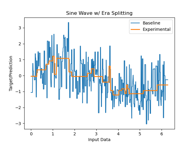
(a) Era Splitting: Plot

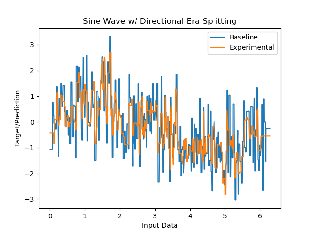
(b) Directional Era Splitting: Plot

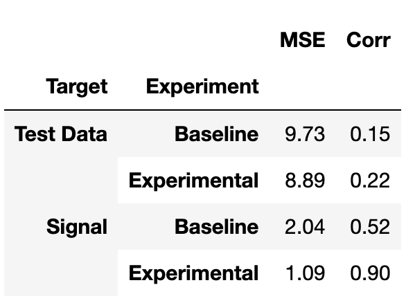
(c) Era Splitting: Table

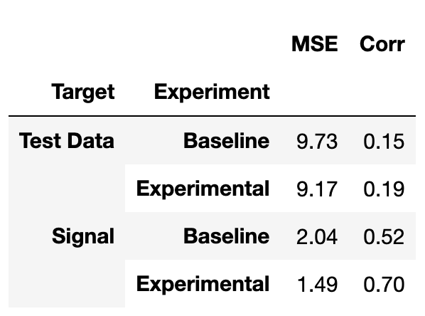
(d) Directional Era Splitting: Table

Figure 6: In this figure we display the results from the shifted since wave experiment. Subplots (a) and (c) in the left column show results for the experimental model implementing the era splitting criterion and subplots (b) and (d) show the the results for the experiment implementing the directional era splitting criterion. For each experiment, we evaluate each model on two versions of the out-of-sample test data. These data sets are listed under ”Target” in the tables. The Test Data is the randomly generated test data set, and Signal uses the sine wave with out any transformation as the target. We see consistent improvement in the evaluation metrics across the board when implementing era splitting or directional era splitting, characterized by lower MSE and higher correlation scores.

The results for the shifted sine wave experiment are presented in figure 6. We first interpret the results of the era splitting experiment, which are shown in the left column of figure 6. What we see is that the baseline model creates a prediction that is very noisy as a function of the input variable, no-doubt owing to the inherent randomness in the target variables. This is compared to the predictions from the experimental model, which implements the era splitting criterion. Qualitatively, we see that this model produces much smoother predictions as a function of the input. Quantitatively speaking, we see improvements in all the evaluation metrics, whether evaluated on the generated test data or on the invariant signal itself. Notably the performance is greatly improved on the invariant signal, while less so for the generated test data. This owes to the fact that there is much randomness in the test data itself that cannot be learned from the training data, since that part of the signal is random. Nevertheless, the experimental model outperforms the baseline naive model by a wide margin.

The directional era splitting model also performs better than the baseline model, but to a lesser extent than the era splitting criterion. Directional era splitting tends to perform closer to the baseline model than regular era splitting in some cases, and we see that happen here.

5.2 Synthetic Memorization Data Set

For this data set, outlined in section 4, we find that a naive baseline model is indeed confounded by the data setup. The era splitting model also performs similarly to the baseline, which good in-sample metric but out of sample the performance is very weak. Meanwhile, the directional era splitting model in able to overcome the confusion of the spurious signal and uncover the invariant predictor.

The main aspects are in-sample model performance compared to out-of-sample performance. What we find is that the naive GBDT model, in this case an LGBM model, performs very well in-sample while only providing chance-level predictions out-of-sample. This confirms that the baseline model has learned the spurious signal and not the invariant one.

Table 1: Experimental Results

	Baseline	Era Splitting	Directional Era Splitting
Correlation (In-Sample)	100%	100%	99%
Correlation (Out-of-Sample)	-2%	2%	93%
Accuracy (In-Sample)	100%	100%	99%
Accuracy (Out-of-Sample)	49%	50%	98%

The experimental model with the era splitting criterion shows the same behavior, however we notice that the the predicted values in the middle pane of figure 7 show that this model is showing less extreme values than the baseline. This model still suffers the same fate as the baseline, in that it is learning the spurious signals and not the invariant predictor.

Finally, we evaluate the directional era splitting model. This model is able to fit the data perfectly in-sample, attaining 99% correlation and 100% accuracy. Stunningly, we also see similar results on the test set: 93% correlation and 98 % accuracy. This indicates that the directional era splitting model is about to effectively ignore the spurious signal and learn the invariant signal from the data, asa evident from the out-of-sample performance, and decision boundary in the right pane of figure 7.

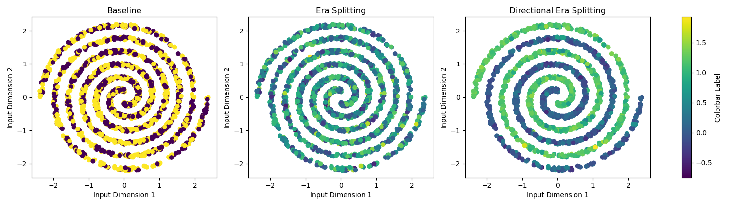
Figure 7: In this figure we plot the input data along the first 2 dimensions, which contains the swirl invariant signal. Each dot is colored depending on the predicted label for that point. This is the decision surface along the first two dimensions. We can ascertain that the baseline model created fairly random scattering of strong predictions across the pane. This means the model did not pick up on this swirl pattern, and based its perfect in-sample prediction score on the remaining features which contained the shifting, but easier signal. Meanwhile we see that the directional era splitting model clearly has learned to differentiate the two arms of the swirl. One arm of the swirl is clearly a lighter color than the other. However the predictions are not as extreme as the baseline, telling a more cautious tale.

In figure 7 we plot the decision surfaces produced by the two models as a function of the first two dimensions of the input data, which contains the invariant signal. What we discern here is that indeed the baseline model was unable to uncover the invariant spiral signal. We can say this because the predictions based on the data along these dimensions appear to be a random scatter. The model clearly is not incorporating the information from these features in the prediction. For the case of vanilla era splitting, we see the same behavior, but with slightly less-confident predictions, judged by the magnitude in the predicted values. Finally, for the directional era splitting model, we see clearly it has learned to differentiate one of the spiral arms from the other with confidence, while not being as confident as the baseline model, which was incredibly confident but very wrong.

5.3 Numerai Data

The Numerai data proved difficult. This data, indeed, is from the ”the hardest data science tournament on the planet”. This is real market data and the prediction problem is notoriously difficult. We don’t have a guarantee, but only an assumption that there is an invariant signal present, linking the input data with the targets consistently over time. An interesting finding from directional era splitting is that there did not exist even one single split from a single feature at the root node which had a consistent direction across all the eras in the training data. This is to say that there wasn’t a single feature which worked in the same way all the time as a linear predictor of the target. See the accompanying code for more details.

The results are not easy to interpret. Overall, the newly developed splitting criteria (by themselves) did not produce models which exceeded the performance of a baseline model. However, owing to the plasticity of the system, we trained models using a linear 60-40 combination of the original splitting criterion with era splitting criterion, and were able to beat the baseline model results in this way. Keep in mind the baseline model is an LGBM model which was found to be a high performer via a large parameter grid search, and the experimental model is built on our HistGradientBoostingRegressor framework. These models are indicated in figure 8. The experimental model was able to exceed the baseline model performance out of sample. We see we have attained a higher mean, median and maximum era-wise correlation with the target, as well as a higher correlation Sharpe.

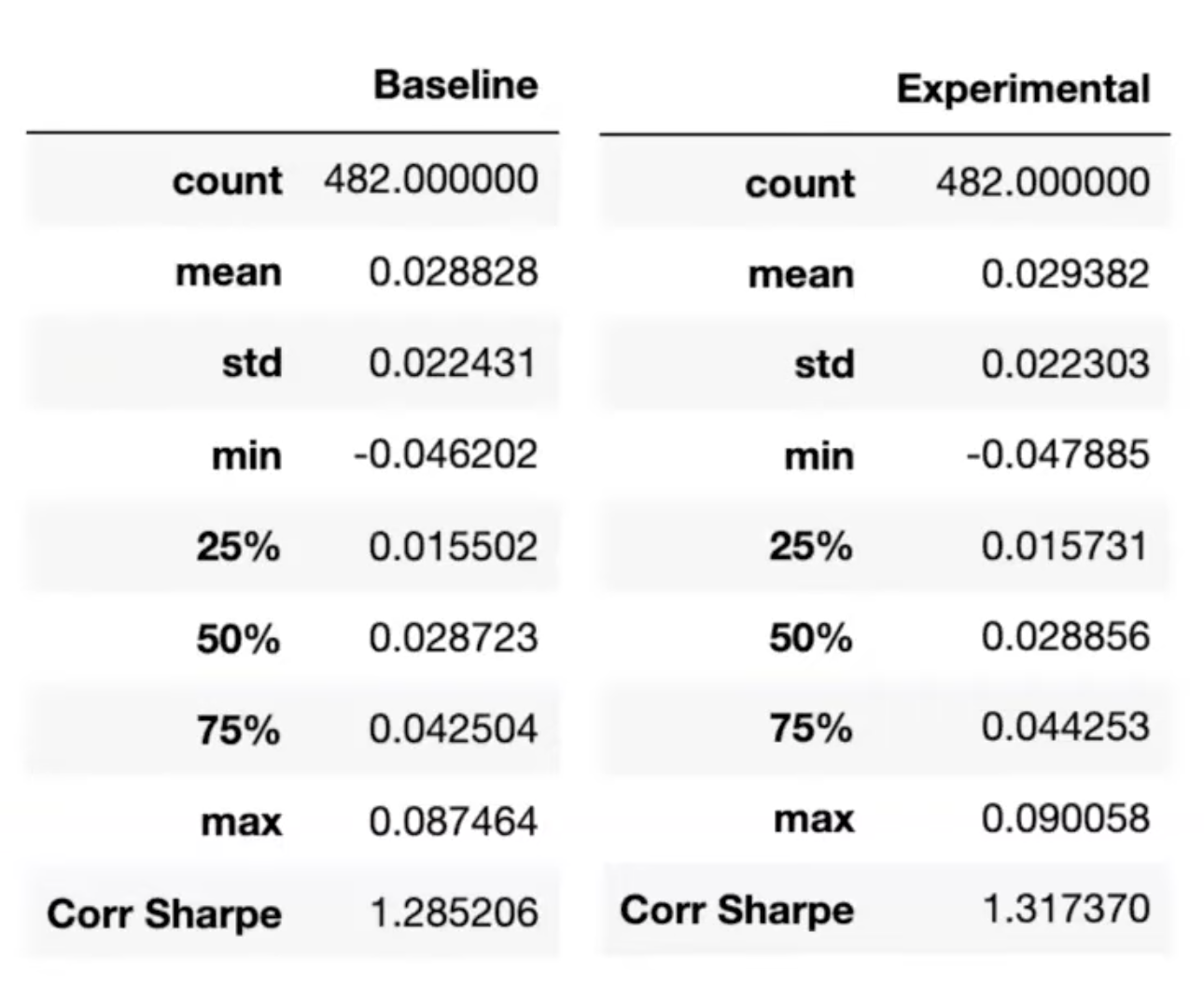
Figure 8: Numerai data results. Here we show the statistics for the era-wise correlations of the baseline model compared to the experimental model. A total of 482 eras went into these calculations. We see the experimental model has a higher mean and lower standard deviation of era-wise correlations, leading to a higher Corr Sharpe for the experimental model. The Corr Sharpe is simply the mean/std. There are other favorable statistics here like higher max and median era-wise correlations as well.

The directional era splitting criterion by itself produced models that came very close to the baseline model’s performance without exceeding it, unfortunately. We were also unable to produce better performance by mixing the criterion with the original as in the above era splitting example. However, we’ve developed an easy-to-use notebook so anyone interested can try their hand at the problem. Indeed there are a lot untested parameter combinations and innovations abound. We encourage the community to help push forward development of these ideas.

6 Discussion

Certain real-world ML problems inherently have a notion of environment or era associated with data. Data is collected from nature in different locations or at different times, and there are distributional shifts in the data generation process from place to place or from time to time. One day it is raining, the other day it is sunny. The emerging field of OOD generalization is concerned with developing ML theory and algorithms to better address this fact, straying from the ERM paradigm. The main assumption of ERM is that the data distribution is the same across time and space. Instead, we assume that data distributions change depending on the environment (or era) the data is drawn from. We’ve been inspired by previous work, which incorporates era-wise information into linear and neural network architectures in order to help the algorithms learn invariant signals and ignore spurious signals that shift from one era to the next.

In this work we addressed the splitting criterion of decision tree based algorithms. Such algorithms include decision trees, random forest and gradient boosted decision trees. The last on this list is currently considered state-of-the-art for many important supervised learning problems, and which output is a weighted average of decision trees. By incorporating era-wise information in the splitting criterion, we integrate that information into the entire model.

We developed two novel splitting criteria, called the era splitting and directional era splitting criterion respectively. We believe that such new splitting criteria can allow the gradient boosted decision tree models to better learn invariant predictive signals from data which has environmental or era-wise distributional shifts. The definitions of the new criteria are described in sections 2 and 3.

In order to test our new criteria for regression we developed a new shifted sine wave model. We also used a synthetic memorization data set that was developed in [Par+20], and we adapted it to a regression objective. Finally, we tested the model on a real-world data set from Numerai for predicting market returns over time. On the shifted sine wave data set era splitting greatly improves out of sample performance. Directional era splitting also improves out of sample performance, but to a lesser extent. For the synthetic memorization data set problem, we found that out of sample correlation and accuracy are improved over the baseline with directional era splitting. A very good result is that directional era splitting was able to attain almost perfect out-of-sample correlation and accuracy, meaning this model was able to effectively completely ignore spurious signals and instead learn the invariant swirl signal. In figure 5 we visualize the decision surface for our two experimental models. Finally, the Numerai data proved most difficult. By blending our new era splitting criterion with the original variance-minimizing criterion, we were able to beat the baseline model in key out-of-sample metrics.

We hope that releasing this paper and code will inspire more to work in this direction, looking for ways to understand OOD generalization in the context of decision trees and gradient boosted decision trees. We did not perform extensive research regarding the parameter $\alpha$ in the Boltzmann operator of the era splitting criterion. This adjustment can alter the perspective, instead of looking for the best average impurity improvement for a split, we can alternatively look at the (smooth) minimum or maximum impurity improvement for each split. We hope a driven researcher will give attention to this in future research. All experiments presented here keep the parameter fixed at zero.

We’ve surmised that evaluating a splitting criterion is effectively a one-dimensional operation. We operate on one feature at a time. Perhaps is is also a drawback when looking for invariant signals, which most likely will be high-dimensional and complex. Is there a way to build invariant trees instead of just invariant splits? This is also motivation for future research.

6.1 Time Complexity

One of the biggest obstacles to the wide-spread adoption of this model is the added time complexity that is added by the era splitting routine. Indeed, one of the main issues with GBDTs in general is that, in order to grow a tree, at each node we must compute the information gain (equation 1) for every potential split in our entire data set. This means we must perform this calculation for every distinct value for every feature in our data. The histogram method in modern software libraries has helped by reducing the number of unique values in the features down to a set parameter value. Setting this parameter to a low value, like 5, can greatly reduce training time. The colsample bytree method also reduces the total number of computations needed by randomly sampling a subset of the features to use to build each tree.

In Era Splitting, we must compute the information gain not once by $M$ times, where $M$ is the number of eras in our training data. For the Numerai data, $M$ takes a value of 478. Run times for this implementation can then be 478 times longer than the baseline model. This becomes prohibitive, as training times for larger models can easily take several days to complete training.

Progress in this area could be rewarding, as long training times will prohibit progress with this algorithm. A simple idea is to regroup the eras into era groups. Naive methods can sometimes lead to increased performance in some settings, although this hasn’t been explored completely.

References

- [Mar52] Harry Markowitz “PORTFOLIO SELECTION*” In The Journal of Finance 7.1, 1952, pp. 77–91 DOI: https://doi.org/10.1111/j.1540-6261.1952.tb01525.x
- [Vap91] V. Vapnik “Principles of Risk Minimization for Learning Theory” In Advances in Neural Information Processing Systems 4 Morgan-Kaufmann, 1991 URL: https://proceedings.neurips.cc/paper_files/paper/1991/file/ff4d5fbbafdf976cfdc032e3bde78de5-Paper.pdf
- [Bre01] Leo Breiman “Random Forests” In Machine Learning 45.1 Kluwer Academic Publishers, 2001, pp. 5–32 DOI: 10.1023/A:1010933404324
- [Fri01] Jerome H. Friedman “Greedy function approximation: A gradient boosting machine.” In The Annals of Statistics 29.5 Institute of Mathematical Statistics, 2001, pp. 1189–1232 DOI: 10.1214/aos/1013203451
- [FF04] Eugene F. Fama and Kenneth R. French “The Capital Asset Pricing Model: Theory and Evidence” In Journal of Economic Perspectives 18.3, 2004, pp. 25–46 DOI: 10.1257/0895330042162430
- [Ped+11] F. Pedregosa et al. “Scikit-learn: Machine Learning in Python” In Journal of Machine Learning Research 12, 2011, pp. 2825–2830
- [CG16] Tianqi Chen and Carlos Guestrin “XGBoost” In Proceedings of the 22nd ACM SIGKDD International Conference on Knowledge Discovery and Data Mining ACM, 2016 DOI: 10.1145/2939672.2939785
- [AL17] Kavosh Asadi and Michael L. Littman “An Alternative Softmax Operator for Reinforcement Learning” In Proceedings of the 34th International Conference on Machine Learning 70, Proceedings of Machine Learning Research PMLR, 2017, pp. 243–252 URL: https://proceedings.mlr.press/v70/asadi17a.html
- [Ke+17] Guolin Ke et al. “LightGBM: A Highly Efficient Gradient Boosting Decision Tree” In Advances in Neural Information Processing Systems 30 Curran Associates, Inc., 2017 URL: https://proceedings.neurips.cc/paper_files/paper/2017/file/6449f44a102fde848669bdd9eb6b76fa-Paper.pdf
- [Arj+20] Martin Arjovsky, Léon Bottou, Ishaan Gulrajani and David Lopez-Paz “Invariant Risk Minimization”, 2020 arXiv:1907.02893 [stat.ML]
- [NAN20] Vaishnavh Nagarajan, Anders Andreassen and Behnam Neyshabur “Understanding the Failure Modes of Out-of-Distribution Generalization” In CoRR abs/2010.15775, 2020 arXiv: https://arxiv.org/abs/2010.15775
- [Par+20] Giambattista Parascandolo et al. “Learning explanations that are hard to vary”, 2020 arXiv:2009.00329 [cs.LG]
- [BGM22] John Blin, John Guerard and Andrew Mark “A History of Commercially Available Risk Models” In Encyclopedia of Finance, Springer Books Springer, 2022, pp. 2275–2311 DOI: 10.1007/978-3-030-91231-4
- [GOV22] Léo Grinsztajn, Edouard Oyallon and Gaël Varoquaux “Why do tree-based models still outperform deep learning on tabular data?”, 2022 arXiv:2207.08815 [cs.LG]
- [Com23] Numerai Community “Super Massive LGBM Grid Search” Accessed on 2023-09-25, 2023 URL: https://forum.numer.ai/t/super-massive-lgbm-grid-search/6463
- [Liu+23] Jiashuo Liu et al. “Towards Out-Of-Distribution Generalization: A Survey”, 2023 arXiv:2108.13624 [cs.LG]