Principal stratification with continuous treatments and continuous post-treatment variables

Abstract

In causal inference studies, interest often lies in understanding the mechanisms through which a treatment affects an outcome. One approach is principal stratification (PS), which introduces well-defined causal effects in the presence of confounded post-treatment variables, or mediators, and clearly defines the assumptions for identification and estimation of those effects. The goal of this paper is to extend the PS framework to studies with continuous treatments and continuous post-treatment variables, which introduces a number of unique challenges both in terms of defining causal effects and performing inference. This manuscript provides three key methodological contributions: 1) we introduce novel principal estimands for continuous treatments that provide valuable insights into different causal mechanisms, 2) we utilize Bayesian nonparametric approaches to model the joint distribution of the potential mediating variables based on both Gaussian processes and Dirichlet process mixtures to ensure our approach is robust to model misspecification, and 3) we provide theoretical and numerical justification for utilizing a model for the potential outcomes to identify the joint distribution of the potential mediating variables. Lastly, we apply our methodology to a novel study of the relationship between the economy and arrest rates, and how this is potentially mediated by police capacity.

1 Introduction and background

In the potential outcome approach to causal inference Rubin, (1974), principal stratification (PS, Frangakis and Rubin,, 2002) is a useful approach to conceptualize the mediating role of intermediate variables in the treatment-outcome relationship (e.g., Ten Have and Joffe,, 2012; Baccini et al.,, 2017; Kim et al.,, 2019). A PS with respect to a mediating variable is a cross-classification of subjects into groups, named principal strata, defined by the joint potential values of that mediating variable under each treatment level. Therefore, principal strata are comprised of units having the same potential values of the mediator, which are not affected by treatment and can therefore be viewed as an intrinsic latent characteristic of the units. Principal causal effects (PCEs), defined as comparisons of potential outcomes under different treatment levels within a principal stratum, provide information on treatment effect heterogeneity with respect to the mediator. Studying the heterogeneity of treatment effects with respect to principal stratum membership is a powerful tool to unveil underlying causal mechanisms Mealli and Mattei, (2012). As an example, one can look at treatment effects within principal strata for which the treatment either does or does not causally affect the mediator, sometimes referred to as associative or dissociative effects. Dissociative PCEs can be interpreted as the principal strata direct effects of the treatment on the outcome not channeled through the mediator, whereas associative PCEs combine both direct and indirect effects of the treatment through the mediating variable VanderWeele, (2008). See Rubin, (2004); Mattei and Mealli, (2011); Baccini et al., (2017) for a discussion. Comparing the magnitude of these two effects can provide insights into whether the treatment effects are mediated or not (e.g., Zigler et al.,, 2012; Forastiere et al.,, 2016).

Principal stratification is well studied for binary treatments and has been applied to a wide range of post-treatment variable types spanning binary, multivariate, continuous and time-dependent mediators. Imbens and Rubin, (1997); Hirano et al., (2000); Mealli and Rubin, (2003); Jin and Rubin, (2008); Sjölander et al., (2009); Frumento et al., (2012); Zigler and Belin, (2012); Mattei et al., 2023a ; Bia et al., (2022). In these settings, assumptions on the treatment assignment mechanism are not sufficient for identification of PCEs, and a number of different assumptions have been proposed to rectify this concern. Arguably the most common of these are monotonicity and exclusion restriction assumptions Angrist et al., (1996); Hirano et al., (2000); Bia et al., (2022), which eliminate certain principal strata and enforce that certain PCEs are zero, and the plausibility of these depends on the empirical setting. Alternative assumptions have been proposed, such as principal ignorability Jo et al., (2011); Jiang and Ding, (2021); Mattei et al., 2023b , or conditional independence between an auxiliary variable and the outcome given principal stratum membership and covariates (e.g., Jiang and Ding,, 2021). Alternatively, if explicit identification is not possible, some authors have derived partial identification results for PCEs as well (e.g., Zhang and Rubin,, 2003; Cheng and Small,, 2006; Imai,, 2008; Lee,, 2009; Mealli and Pacini,, 2013; Mealli et al.,, 2016; Yang and Small,, 2016). If structural assumptions are not feasible to obtain nonparametric identification, one alternative is to obtain identification through a combination of structural assumptions and parametric assumptions (e.g., Hirano et al.,, 2000; Mattei and Mealli,, 2007; Jin and Rubin,, 2008; Ma et al.,, 2011; Schwartz et al.,, 2011; Bartolucci and Grilli,, 2011; Frumento et al.,, 2012; Zigler and Belin,, 2012; Kim et al.,, 2019). For a comprehensive overview of identification results for PCEs with binary treatments, we point readers to Jiang and Ding, (2021). In addition to the binary treatment setting, extensions exist for both longitudinal treatments Frangakis et al., (2004); Ricciardi et al., (2020) and multi-valued treatments Cheng and Small, (2006); Feller et al., (2016).

Despite this existing work, a critical gap in the literature remains, which is how to utilize principal stratification with continuous treatments. While seemingly a simple extension, we will see that continuous treatments pose a number of serious challenges to principal stratification that are unique to this setting, both in terms of identification strategies and inferential approaches. Addressing these issues is critically important as studies with continuous treatments are ubiquitous across a range of applied areas. The combination of a continuous treatment and a continuous mediator raises challenges because there are infinitely many principal strata defined by the treatment-mediator trajectories. Additionally, principal causal estimands are treatment-response functions for the subpopulation of units with specific treatment-mediator trajectories, rendering the definition of associative and dissociative PCEs, or other scientifically meaningful estimands, difficult. Even if well-defined and scientifically meaningful estimands are found, identification of such estimands is increasingly difficult in this setting, and existing assumptions such as monotonicity or exclusion restrictions do not lead to nonparametric identification of treatment effects.

In this manuscript, we make a number of important contributions to the literature on principal stratification. First, we develop a framework for principal stratification with continuous treatments, and provide innovative estimands that can meaningfully capture both associative and dissociative principal causal effects (among others) with a continuous mediator to shed light on its mediating role. While we focus on the specific scenario of continuous treatments and continuous mediators, these ideas apply to any situation with a continuous treatment, regardless of the type of mediator. Additionally, we highlight difficulties with identification in this more complex scenario that are caused by the inability to nonparametrically identify the associations between potential mediator values at different treatment levels. We provide theoretical justification for incorporating an outcome model to identify these parameters by showing that these association parameters can be consistently estimated if an outcome model is correctly specified. This not only provides a novel identification result for the continuous treatment setting, but it provides theoretical justification for outcome model-based approaches that have been used in the binary treatment setting, which only had heuristic justification previously. Finally, we develop a nonparametric Bayesian approach to estimation in this scenario, which alleviates concerns due to model misspecification, and helps to separate units into different principal strata. Specifically, we specify a Gaussian process for the distribution of potential mediators, in conjunction with a Dirichlet process mixture model for the mean of the mediator distribution. Not only is this model flexible, but it also clusters units based on their treatment-mediator trajectories, which can help identify different principal strata of interest. We confirm our theoretical results in simulation, and show that the proposed approach is able to estimate meaningful principal causal effects. Lastly, we study an important problem in criminology, which is how the economic prosperity of a region affects arrest rates in that area. We apply our proposed methodology to better understand this effect, and whether that effect is channelled through changes in police capacity in the region of interest.

2 Principal stratification framework with continuous treatments and intermediate variables

Throughout, we assume that we observe $n$ independent observations given by $\bm{D}_{i}=(Y_{i},S_{i},T_{i},\bm{X}_{i})$ for $i=1,\dots,n$. These contain the observed outcome $Y_{i}$, the observed mediator $S_{i}$, the treatment $T_{i}$, and a $p-$dimensional vector of pre-treatment characteristics for unit $i$, given by $\bm{X}_{i}$. We focus on studies where both the treatment, $T_{i}$, and the mediator, $S_{i}$ are continuous variables with support in (proper) subsets of the real line, denoted by $\mathcal{T}$ and $\mathcal{S}$, respectively. We postulate the existence of a set of potential outcomes for both the mediator, $S_{i}(t)$, and for the main endpoint, $Y_{i}(t)$, for $t\in\mathcal{T}$. These denote the potential values of the mediator and the outcome that would be observed under treatment level $t$. Denoting potential mediators and outcomes in this way implicitly makes the Stable Unit Treatment Value Assumption (SUTVA, Rubin,, 1980) which states that $(i)$ there is no “interference” in the sense that potential intermediate and primary outcome values from unit $i$ do not depend on the treatment applied to other units, and $(ii)$ there are “no multiple versions” of the treatment, such that whenever $t=t^{\prime}$, $S_{i}(t)=S_{i}(t^{\prime})$ and $Y_{i}(t)=Y_{i}(t^{\prime})$. Under SUTVA, we have that $S_{i}=S_{i}(T_{i})$ and $Y_{i}=Y_{i}(T_{i})$, which links the potential outcomes to the observed outcomes. For notational simplicity we let $\bm{S}_{i}=\{S_{i}(t)\}_{t\in\mathcal{T}}$ denote the individual treatment-mediator function, which is the trajectory of the potential mediator over the range of values of the treatment for unit $i$. To simplify the notation, we drop the $i$ subscript in what follows unless explicitly needed.

2.1 Principal Stratification and Causal Estimands

Information on total effect of the treatment $T$ on the outcome $Y$ can be obtained by looking at the average dose–response function, given by $\mu(t)=E\left[Y(t)\right]$, for $t\in\mathcal{T}$. In this manuscript, however, we are interested in understanding the extent to which the average dose–response function is modified by the potential intermediate variables, $S(t)$, which is known as principal stratification Frangakis and Rubin, (2002). The basic principal stratification with respect to the continuous post-treatment variable, $\bm{S}$, is the partition of units into subpopulations, referred to as (basic) principal strata, where all units have the same treatment-mediator trajectory, i.e. $\{i:\bm{S}_{i}=\bm{s}\}$ for some $\bm{s}$. Therefore principal strata can be viewed as mediator trajectories over the possible values of the treatment, essentially describing how the units react to changes in the levels of the treatment in terms of the mediating variable. In principal stratification analysis, the causal estimands of interest are principal causal effects (PCEs), which are local causal effects for units belonging to a specific principal stratum or union of principal strata. In our setting, a natural estimand would be the average principal strata exposure-response curve within a particular principal stratum, given by

$$\mu(t,\bm{s})=E[Y(t)\mid\bm{S}=\bm{s}]\text{ for }t\in\mathcal{T}.$$

There are infinitely many choices for $\bm{s}$, and it is not clear which ones are of most interest. One option relevant to mediation analyses is to define unions of principal strata that highlight associative and dissociative causal effects. Dissociative principal strata exposure-response curves are those for principal strata where the trajectory of the mediator is, at least approximately, constant. Associative principal strata are those for which the trajectory of the mediator is not constant and there is some impact of the treatment on the mediator. Towards this end, we propose to construct unions of principal strata and look at estimands of the form

$$E[Y(t)\mid a<g(\bm{S})<b],$$

as many principal strata of interest can be expressed as the set of individuals for whom $a<g(\bm{S})<b$, for suitable functions $g(\cdot)$. Many features of the potential intermediate variables, such as the shape, slope, range, or more complex estimands can be written in this format, and the choice of function depends on the empirical application and what scientific questions are being addressed. If interest lies in associative and dissociative effects, then one could look at principal strata defined by $g(\bm{S})\equiv\text{range}(\bm{S})=\max_{t\in\mathcal{T}}S(t)-\min_{t\in\mathcal{T}}S(t)$. One could focus on effects of the form $E[Y(t)\mid\text{range}(\bm{S})\leq\epsilon]\ \forall\ t,$ which looks at the exposure-response curve among units for which there is little to no effect of $T$ on $\bm{S}$. This would be analogous to a direct effect in this subpopulation whose value of $\bm{S}$ is unaffected by treatment (dissociative PCE). Alternatively, one can examine $E[Y(t)\mid\text{range}(\bm{S})\geq\delta]\ \forall\ t$, to see the exposure-response curve among units for which there is a large effect of $T$ on $S$ (associative PCE). Alternative options such as the average absolute derivative of this curve, defined by $g(\bm{S})=\int_{\mathcal{T}}|S^{\prime}(t)|\ dt$ could be used to construct similar associative and dissociative effects.

2.2 Assumptions and identification

In the potential outcome approach, inference on causal effects first requires assumptions on the treatment assignment mechanism. We first assume strong unconfoundedness:

Assumption 1

(Strong unconfoundedness). The assignment mechanism is strongly unconfounded, given pre-treatment variables $\bm{X}$, if

$$\{S(t),Y(t)\}_{t\in\mathcal{T}}\mathchoice{\mathrel{\hbox to0.0pt{$\displaystyle\perp$\hss}\mkern 2.0mu{\displaystyle\perp}}}{\mathrel{\hbox to0.0pt{$\textstyle\perp$\hss}\mkern 2.0mu{\textstyle\perp}}}{\mathrel{\hbox to0.0pt{$\scriptstyle\perp$\hss}\mkern 2.0mu{\scriptstyle\perp}}}{\mathrel{\hbox to0.0pt{$\scriptscriptstyle\perp$\hss}\mkern 2.0mu{\scriptscriptstyle\perp}}}T\mid\bm{X}.$$

We also require that the treatment assignment mechanism is probabilistic.

Assumption 2

(Overlap). For all possible values of the pre-treatment variables $\bm{X}$, the conditional probability density function of receiving any possible treatment level $t\in\mathcal{T}$ given $\bm{X}$ is positive.

The overlap assumption guarantees that each unit has a non-zero probability to be exposed to each treatment level for all possible values of pre-treatment variables, at least in large samples. Strong unconfoundedness requires that the treatment $T$ is independent of the entire set of potential mediators and outcomes. It holds by design in randomized experiments, where the treatment assignment mechanism is known and under the control of the researcher, but it might be debatable in observational studies. In observational studies, its plausibility strongly depends on the observed covariates and on subject matter knowledge, which may provide convincing arguments that all the relevant confounders have been observed. It implies that there exist no additional unmeasured variables that confound the treatment - mediator and treatment - outcome relationships.

In principal stratification analysis, strong unconfoundedness is key because it has important implications that help to identify principal strata exposure-response curves. Although we cannot observe the principal stratum membership for any unit, strong unconfoundedness guarantees that principal strata trajectories, $\bm{S}$, have the same distribution across treatment levels, within cells defined by pre-treatment variables, $\bm{X}$. Moreover, strong unconfoundedness implies that $\{Y(t)\}_{t\in\mathcal{T}}\mathchoice{\mathrel{\hbox to0.0pt{$\displaystyle\perp$\hss}\mkern 2.0mu{\displaystyle\perp}}}{\mathrel{\hbox to0.0pt{$\textstyle\perp$\hss}\mkern 2.0mu{\textstyle\perp}}}{\mathrel{\hbox to0.0pt{$\scriptstyle\perp$\hss}\mkern 2.0mu{\scriptstyle\perp}}}{\mathrel{\hbox to0.0pt{$\scriptscriptstyle\perp$\hss}\mkern 2.0mu{\scriptscriptstyle\perp}}}T\mid\{S(t)\}_{t\in\mathcal{T}},\bm{X}$. Therefore, units belonging to the same principal stratum and with the same value of the covariates but exposed to different treatment levels can be compared to draw valid inference on causal effects. While necessary for inference, strong unconfoundedness and overlap are not sufficient for nonparametric identification of principal causal effects. We show in Appendix A that under these two assumptions, we are able to write $E[Y(t)\mid a<g(\bm{S})<b]$ as

$$\int_{\bm{x}}\int_{\bm{s}}E[Y\mid T=t,\bm{S}=\bm{s},\bm{X}=\bm{x}]\dfrac{f(\bm{s}\mid T=t,\bm{X}=\bm{x})1(a<g(\bm{s})<b)}{P(a<g(\bm{S})<b\mid T=t,\bm{X}=\bm{x})}\,d\bm{s}\,dF_{\bm{X}\mid a<g(\bm{S})<b}(\bm{x}),$$ (1)

where $f(\bm{s}\mid T=t,\bm{X}=\bm{x})$ is the conditional density function of the potential mediators. If we could observe the principal stratum $\bm{S}$ for each unit, we could identify both $E[Y\mid T=t,\bm{S}=\bm{s},\bm{X}=\bm{x}]$ and $f(\bm{s}\mid T=t,\bm{X}=\bm{x})$, which would imply nonparametric identification of the principal causal effect. However, this quantity is only partially observed as we only observe one $S$ associated with the observed value of the treatment $T$, and therefore we need to impose further assumptions to draw inference on principal strata exposure-response curves. Frequently in the principal stratification literature, additional structural assumptions are placed on the potential mediators or outcome, such as monotonicity or exclusion restrictions, to reduce the number of principal strata and obtain identification. While we will see later that monotonicity can be utilized in this setting, these assumptions are still insufficient for identification without additional assumptions on the distribution of the principal strata. In this manuscript, we utilize parametric assumptions in both the outcome model and the model for the principal strata to identify causal effects. If these parametric assumptions are satisfied, then under certain conditions we will be able to learn the distribution of the missing potential mediators, and identify all terms in (1). While this strategy has been used heuristically with empirical evidence to suggest it works (Bartolucci and Grilli,, 2011; Schwartz et al.,, 2011), no theoretical evidence supporting its use has been shown. In Section 4, we provide theoretical support to this strategy by showing that a correctly specified outcome model leads to identification of the dependence among the distinct potential mediators, which leads to identification of PCEs, but only when the potential mediators have an effect on the outcome.

3 Nonparametric Bayesian modeling framework

We propose to use a Bayesian approach to inference, which is often adopted in PS analysis where inference involves techniques for incomplete data (e.g. Jin and Rubin,, 2008; Schwartz et al.,, 2011; Kim et al.,, 2019; Mattei et al., 2023a, ). Conditioning on the observed distribution of the covariates, Bayesian PS analysis requires the specification of two sets of models: one for the distribution of principal strata conditional on the covariates, and one for the distribution of potential outcomes conditional on the principal strata and covariates. Both of these models are crucially important for updating $S(t)$ for $t\in\mathcal{T}$, which define principal strata membership for each unit in the sample.

Under the assumption that potential outcomes for the primary endpoint are conditionally independent given principal strata and covariates, we directly specify the marginal models $Y(t)\mid\bm{S},\bm{X}$. Under strong unconfoundedness and overlap, this is equivalent to positing a model for the observed outcome conditional on the principal strata and covariates, $Y\mid T=t,\bm{S},\bm{X}$. The principal strata model, however, requires one to posit a model for the full joint distribution of the potential intermediate values. Given these two sets of models, we derive the posterior distributions of the causal estimands of interest using a Markov chain Monte Carlo (MCMC) algorithm with data augmentation. Specifically, because we are only able to observe the potential intermediate variable at the observed treatment levels, we utilize a data augmentation step that imputes the missing values of the potential intermediate variables at each step of the MCMC algorithm, and all parameters are updated conditionally on these values. In what follows, we describe each of the outcome and potential intermediate models separately and then discuss how the posterior distributions of these model parameters can be used to estimate principal causal effects.

3.1 Nonparametric Bayesian isotonic regression for potential intermediate

We first need to posit a model for the joint distribution of the potential intermediate values, conditional on the observed covariates, i.e. $\bm{S}\mid\bm{X}$. There are a number of important features that we want this model to have. We want to estimate this model as flexibly as possible so that we do not misspecify the distribution of the potential intermediate values, which would lead to incorrect imputations of the missing potential intermediate values and estimates of principal causal effects. We also want to be able to incorporate some degree of monotonicity into this model as we believe the relationship between the treatment and intermediate variables in our setting to be monotonic, and incorporating this assumption could improve efficiency. Lastly, we want our model to induce clustering of the units in the sample, as this will help to separate them into different principal strata. We first assume that the set of potential intermediate values follows a Gaussian process defined by

$$\bm{S}\mid\bm{X}=\bm{x}\sim\mathcal{GP}(m(t,\bm{x}),K(t,t^{\prime})).$$

The mean function $m(t,\bm{x})$ allows the mean of $S(t)$ to vary by both $t$ and $\bm{x}$. We can use a standard kernel function, such as

$$K(t,t^{\prime})=\sigma_{S}^{2}\ e^{-\frac{(t-t^{\prime})^{2}}{\rho}},$$

which enforces that two values of the potential intermediate at treatment values $t$ and $t^{\prime}$ will be more correlated when the difference $t-t^{\prime}$ is small in magnitude. An important parameter in this specification is $\rho$, which dictates the magnitude of this correlation, and we discuss it further in subsequent sections. In practice, we discretize the set of potential intermediate values to look at and only consider $\bm{t}=[t_{1},t_{2},\dots,t_{M}]$. The Gaussian process specification above implies that

$$\Big{(}S(t_{1}),\dots,S(t_{M})\mid\bm{X}=\bm{x}\Big{)}\sim\mathcal{N}\Big{(}(m(t_{1},\bm{x}),\dots,m(t_{M},\bm{x})),\bm{\Sigma}_{S}\Big{)},$$

where the $(i,j)$ element of $\bm{\Sigma}_{S}$ is given by $K(t_{i},t_{j})$. We first simplify the mean function as

$$m(t,\bm{x})=\phi(t)+\bm{x\alpha}.$$

Note that nonlinear effects of the covariates in $\bm{x}$ could be easily incorporated here as well, but our focus will be on the $\phi(\cdot)$ component of the model that shows how the potential intermediate variable is related to the treatment level $t$. Additionally, this is the part of the model where we can impose a monotonicity constraint, as well as clustering to identify different units in terms of how their intermediate variable is affected by treatment.

There is an extensive literature on Bayesian isotonic regression, which can be used to ensure that $\phi(t)$ is increasing in $t$. Similar to Neelon and Dunson, (2004) we let this function be piecewise linear, and we additionally incorporate nonparametric Bayesian prior distributions on the coefficients to induce clustering. This is somewhat related to the nonparametric prior distributions used in Wilson et al., (2020), however, clustering there was done at the coefficient level, while our prior will induce clustering at the unit level. Specifically, we represent this function using the basis function representation $\phi(t)=\sum_{j=1}^{J}d_{j}(t)\theta_{j}=\bm{d}(t)\bm{\theta}.$ If we have knot locations $\kappa_{1},\dots,\kappa_{J-1}$, then we can define basis functions as $d_{1}(t)=t,d_{2}(t)=(t-\kappa_{1})_{+},\dots,d_{J}(t)=(t-\kappa_{J-1})_{+}$ to obtain a piecewise linear function. To ensure monotonicity of this function, we need $\theta_{1}\geq 0,\theta_{1}+\theta_{2}\geq 0,\dots,\theta_{1}+\dots+\theta_{J}\geq 0$. Alternatively, we need $\bm{A\theta}\geq\bm{0}$, where

$$\bm{A}=\begin{pmatrix}1&0&0&\cdots&0\\ 1&1&0&\cdots&0\\ \vdots&\vdots&\cdots&\ddots&\vdots\\ 1&1&1&\cdots&1\end{pmatrix}.$$

We can re-write our basis expansion as $\phi(t)=\bm{d}(t)\bm{A}^{-1}\bm{A}\bm{\theta}=\bm{b}(t)\bm{\eta}$, where $\bm{\eta}=\bm{A}\bm{\theta}$. To ensure monotonicity, we simply must restrict that $\eta_{j}\geq 0$ for all $j$. We can enforce this through our prior distribution, by specifying a truncated multivariate normal distribution for $\bm{\eta}$ that truncates all values to be on the positive real line. Additionally, we can incorporate an intercept as the first basis function, but we do not care whether the intercept is positive or negative, and therefore it will not be truncated below at zero.

To achieve clustering and model flexibility, we allow the parameters dictating this association, given by $\bm{\eta}$, to vary by individual and have the following hierarchical formulation:

$$\bm{\eta}_{i} \sim G,\quad G=\sum_{c=1}^{\infty}\pi_{c}\delta_{\bm{\xi}_{c}},\quad\bm{\xi}_{c}\sim G_{0}$$

$$\pi_{1} =V_{1},\quad\pi_{c}=V_{c}\prod_{j<c}(1-V_{j}),\quad V_{j}\sim Beta(1,\kappa)$$

This is equivalent to say that $G\sim DP(\kappa,G_{0})$, or that $G$ follows a Dirichlet process with concentration parameter $\kappa$ and base distribution $G_{0}$ (Ferguson,, 1973; Sethuraman,, 1994). In practice, we can set an upper value $C$ on the number of mixture components to approximate the infinite mixture model. A well-known consequence of this Dirichlet process prior is that it induces clustering as some observations will have the same value of $\bm{\eta}_{i}$. The size and number of clusters is dictated by the concentration parameter $\kappa$, as smaller values of $\kappa$ will lead to fewer clusters with more observations in them. This is important in our setting as we are aiming to find which observations are in each principal strata, and this nonparametric prior distribution allows observations to have differential effects of the treatment on the potential intermediate, which will lead to them being members of different strata. An additional modification that we choose to make to this prior is to set $\bm{\xi}_{1}=\bm{0}$, which ensures that the first cluster will have a flat $\phi(t)$ function. This cluster represents observations for which the treatment does not affect the potential intermediate variable, which represents an important principal strata of interest. Lastly, we place a gamma prior distribution on $\kappa$ to let the data inform the degree of clustering.

3.2 Parametric outcome model

Now we focus attention on the model for the observed outcome, which plays two key roles in the estimation of principal causal effects. The more obvious of these two facets of the model is that this is where we estimate the impact of the treatment on the outcome. The second important role is that the outcome model, particularly the manner in which we include the principal strata $\bm{S}$ into this model, affects both the imputation of the unobserved potential intermediates and the updating of the correlation parameter $\rho$ that dictates the correlation among the potential intermediates. We provide more details on the nature of this in Section 4. We can specify the following model for the outcome:

$$E[Y(t)\mid\bm{S}=\bm{s},\bm{X}=\bm{x}]=E[Y\mid T=t,\bm{S}=\bm{s},\bm{X}=\bm{x}]=f(t,\bm{s})+\bm{x\gamma},$$

where again we have included the covariates linearly, but nonlinear models for the covariates could be adopted in a straightforward manner. Of most importance for estimating principal causal effects, is how to specify the $f(t,\bm{s})$ function. One difficulty is that $\bm{s}$ is a functional predictor, though a number of approaches have been developed for scalar-on-function regression; see Reiss et al., (2017) for a review. The simplest way to address this is through a distributed lag model, such as

$$f(t,\bm{s})=\lambda(t)+\sum_{t^{\prime}}\beta(t^{\prime})S(t^{\prime}).$$

While commonly used in scalar-on-function regression, this model is overly simplistic for our situation as it assumes that the effect of $\bm{S}$ on $Y$ is the same, regardless of the value of $t$. This ensures that the treatment effect is identical across all principal strata, however, our goal is to see if the treatment effect varies by strata. A natural extension to this model is to posit a model of the form

$$f(t,\bm{s})=\lambda(t)+\sum_{t^{\prime}}\beta(t,t^{\prime})S(t^{\prime}),$$

which allows the effect of $\bm{S}$ to depend on $t$. The only thing left to specify is how to estimate the $\beta(t,t^{\prime})$ function. We expect this function to be smooth with respect to both $t$ and $t^{\prime}$. This problem has been encountered in a different context in environmental statistics, and has been addressed by letting this parameter follow a Gaussian process prior (Warren et al.,, 2022) or by letting this function be represented as a sum of basis functions that are chosen a priori (Chen et al.,, 2019). We adopt the latter approach to avoid the large computational burden associated with the Gaussian process prior specification. The simplest version of this approach would be to let $\beta(t,t^{\prime})=\zeta_{0}+\zeta_{1}t+\zeta_{2}t^{\prime}$, though extensions to nonlinear functions of $t$ and $t^{\prime}$ are straightforward.

3.3 Posterior inference

We estimate the aforementioned models within the Bayesian paradigm and therefore inference on all treatment effects of interest will be based on the posterior distribution of the unknown parameters. As a reminder, our estimand $E[Y(t)\mid a<g(\bm{S})<b]$ can be written as in Equation (1). Note that each of the conditional expectations and densities in Equation (1) is a function of the unknown parameters for which we have a posterior distribution. The outer expectation taken over the distribution of $\bm{X}$ given $a<g(\bm{S})<b$ can be approximated by using the empirical distribution of the covariates among the units in the sample for which $a<g(\bm{S})<b$. Specifically, if we let the superscript $(b)$ denote the $b^{th}$ posterior sample of an unknown quantity, then we can calculate

$$\Bigg{(}\frac{1}{\sum_{j=1}^{n}\omega_{j}^{(b)}1(a<g(\bm{S}_{j}^{(b)})<b)}\Bigg{)}\Bigg{\{}\sum_{i=1}^{n}\omega_{i}^{(b)}1(a<g(\bm{S}_{i}^{(b)})<b)$$

$$\times \int_{\bm{s}}E^{(b)}(Y\mid T=t,\bm{X}=\bm{X}_{i},\bm{S}=\bm{s})\frac{f^{(b)}(\bm{s}\mid T=t,\bm{X}=\bm{X}_{i})1(a<g(\bm{s})<b)}{P^{(b)}(a<g(\bm{S})<b|T=t,\bm{X}=\bm{X}_{i})}d\bm{s}\Bigg{\}}.$$

Here we have introduced weights for each data point $(\omega_{1}^{(b)},\omega_{2}^{(b)},\dots\omega_{n}^{(b)})\sim\text{Dirichlet}(1,1,\dots,1)$ to account for uncertainty stemming from the observed sample being used to approximate the expectation over the covariate distribution as in the Bayesian bootstrap (Rubin,, 1981). This is a standard approach to accounting for covariate uncertainty for population estimands in Bayesian causal inference (Linero and Antonelli,, 2023). In practice, the integral with respect to $\bm{s}$ is done using a Monte Carlo approximation, which we outline in Appendix A. We obtain this quantity for all posterior samples $b=1,\dots,B$, and inference can proceed using traditional Bayesian approaches once a posterior distribution is obtained.

We do not discuss technical details of Markov chain Monte Carlo (MCMC) sampling or other computational concerns here, and these can be found in Appendix C. All parameters have closed form full conditional distributions, which facilitates sampling through a Gibbs sampler. Updating the correlation parameter for the intermediates, denoted by $\rho$, is greatly improved by utilizing a conditional distribution that marginalizes over the potential intermediates $\bm{S}$. We have derived this marginal distribution in Appendix B. Additionally, prior distributions are assumed to be relatively flat, non-informative prior distributions unless specified otherwise above.

4 Using the outcome model to identify correlation between principal strata

One difficulty in the estimation of principal causal effects in this setting is that we do not know the underlying correlation between $S_{i}(t)$ and $S_{i}(t^{\prime})$, and we only get to observe one value of the intermediate for each unit in the sample. In prior work on principle stratification, this parameter is frequently treated as a sensitivity parameter and the analysis is run for different values of the sensitivity parameter to see how results vary. In other work, it is assumed that the correlation can be learned by incorporating information from the outcome model, but only heuristic arguments for this strategy have been made. Throughout the manuscript, we take the approach of learning the correlation through information from the outcome model, and in this section, we provide justification for this procedure.

For simplicity, in this section, we focus on $P(\bm{S},\rho|\mathcal{D})$ the posterior distribution of $(\bm{S},\rho)$ given the observed data, and treat the other model parameters as fixed at their true values. The same ideas would hold if the other model parameters were being estimated simultaneously, but our goal here is to show the interplay between $\rho$ and the outcome model, and uncover when and how the outcome model informs this parameter. To study what happens to the correlation parameter, we can examine $P(\rho|\mathcal{D})$, the marginal posterior of the correlation parameter. We show in Appendix B that this marginal posterior is given by

$$P(\rho|\mathcal{D}) =P(\rho)\left\{\prod_{i=1}^{n}\bigg{(}1+\frac{\bm{\beta}_{i}^{T}\widetilde{\bm{\Sigma}}_{si}\bm{\beta}_{i}}{\sigma^{2}}\bigg{)}^{-1/2}\right\}$$

$$\times\ \text{exp}\Bigg{\{}-\frac{1}{2}\Bigg{[}\widetilde{\bm{\mu}}_{si}^{T}\widetilde{\bm{\Sigma}}_{si}\widetilde{\bm{\mu}}_{si}-\bigg{(}\frac{\widetilde{Y}_{i}\bm{\beta}_{i}}{\sigma^{2}}+\widetilde{\bm{\Sigma}}_{si}^{-1}\widetilde{\bm{\mu}}_{si}\bigg{)}^{T}\bigg{(}\frac{\bm{\beta}_{i}\bm{\beta}_{i}^{T}}{\sigma^{2}}+\widetilde{\bm{\Sigma}}_{si}^{-1}\bigg{)}^{-1}\bigg{(}\frac{\widetilde{Y}_{i}\bm{\beta}_{i}}{\sigma^{2}}+\widetilde{\bm{\Sigma}}_{si}^{-1}\widetilde{\bm{\mu}}_{si}\bigg{)}\Bigg{]}\Bigg{\}}$$

Here, we have used that $\widetilde{Y}_{i}=Y_{i}-\lambda(T_{i})-\bm{X}_{i}\bm{\gamma}$. We have also adopted the notation that $\bm{\beta}_{i}=(\beta(T_{i},t_{1}),\dots,\beta(T_{i},t_{M}))$. We also defined the mean and variance of the conditional distributions of the potential intermediates $\bm{S}_{i}$ given $S_{i}$, the observed intermediate, as

$$\widetilde{\bm{\mu}}_{si} =m(\bm{t},\bm{X}_{i})+\bm{\Sigma}_{i.}(S_{i}-m(T_{i},\bm{X}_{i}))/\sigma_{S}^{2}$$

$$\widetilde{\bm{\Sigma}}_{si} =\bm{\Sigma}_{S}-\bm{\Sigma}_{i.}\bm{\Sigma}_{i.}^{T}/\sigma_{S}^{2}$$

where here $\bm{\Sigma}_{i.}$ is a vector of values given by $K(T_{i},\bm{t})$. Note that while not explicitly stated, both $\widetilde{\bm{\mu}}_{si}$ and $\widetilde{\bm{\Sigma}}_{si}$ are functions of $\rho$.

This result has a number of important implications. For one, it greatly facilitates sampling as we have found that MCMC sampling algorithms have greatly improved performance and require far fewer iterations when iteratively sampling between $P(\rho|\mathcal{D})$ and $P(\bm{S}|\rho,\mathcal{D})$ instead of a standard Gibbs sampling algorithm that iterates between $P(\rho|\bm{S},\mathcal{D})$ and $P(\bm{S}|\rho,\mathcal{D})$. Of more relevance to this section is that it also has consequences for understanding identification of $\rho$. One can see from the expression that if $\bm{\beta}_{i}=\bm{0}$ for all $i$, the posterior distribution reduces to $P(\rho)$, the prior distribution. This shows that we have no information in the data to learn about $\rho$ if the intermediate variable does not affect the outcome. If, however, there is an effect of the intermediate on the outcome, then there exists information in the data to estimate this parameter.

It is then of interest to study whether the information from the outcome model is correct in the sense that our posterior will concentrate around the true value of $\rho$ when the intermediate variable affects the outcome. We denote the true value of the correlation parameter by $\rho^{*}$. To examine this, we look at the posterior mode for $P(\rho|\mathcal{D})$ to see if the posterior mode converges to $\rho^{*}$. In what follows, we show that asymptotically, the derivative of the marginal posterior is zero at $\rho^{*}$.

Theorem 1: If the outcome model is correctly specified, then

$$\lim_{n\rightarrow\infty}\frac{dP(\rho|\mathcal{D})}{d\rho}\bigg{|}_{\rho=\rho^{*}}=0.$$

A proof of this can be found in Appendix B. This shows that $\rho^{*}$ is an extreme point of the posterior distribution of $\rho$ in large samples, which indicates that it is the maximizing value of this posterior distribution. This shows that not only does the outcome model provide information for estimating $\rho$, but it will lead to consistent estimates of $\rho$. Note that while we have simplified the correlation structure to depend on a single parameter, $\rho$, the same result would hold regardless of the structure of $\bm{\Sigma}_{S}$. The result only depends on correctly specifying the outcome model. If the outcome model is misspecified, the limiting value of the posterior would depend on both the true correlation structure and the variability of the approximation error present due to model misspecification. One final point to make is that the shape of the posterior distribution depends on the magnitude of $\bm{\beta}_{i}$ for $i=1,\dots,n$. Figure 1 shows $P(\rho|\mathcal{D})$ averaged over 100 data sets of size $n=500$, under three scenarios for the true effect of the intermediate on the outcome. We set $\bm{\beta}_{i}=c\bm{1}_{M}$ and varied $c\in\{0.05,0.15,0.25\}$. We see that the posterior is maximized at the true value of 3, but the shape of the posterior is greatly affected by the magnitude of $\bm{\beta}_{i}$. As the effect of the intermediate on the outcome becomes larger, there is more information to update $\rho$ and the posterior becomes more concentrated. While we assumed all other parameters were fixed and known here, we also see this empirically in Section 5 when all parameters are estimated simultaneously.

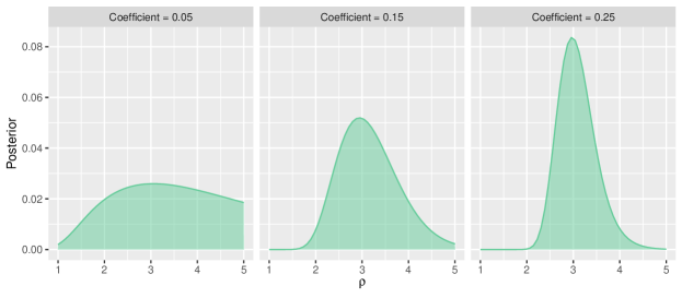
Figure 1: Average marginal posterior distribution across 100 simulated data sets when $\rho^{*}=3$. Each panel corresponds to a different magnitude of association between the intermediate and the outcome.

5 Simulation studies

Here we investigate the performance of the proposed approach to target both principal and average causal effects. Throughout, we set $n=500$ and $p=5$, though we include additional results for larger sample sizes in Appendix D. The main conclusions from the simulation study hold regardless of the sample size. The covariates are generated from independent standard normal distributions. The treatment is generated from a normal distribution with mean $0.15X_{1}+0.25X_{2}$ and variance 0.5. We discretize the set of $t$ values considered to 10 locations on an equally spaced grid between -1.15 and 1.15. The potential intermediate $\bm{S}=(S(t_{1}),\dots,S(t_{10}))$ is generated from a multivariate normal distribution with mean and covariance defined in Section 3.1. We vary the parameter of the kernel function that dictates this covariance $\rho\in\{3,8\}$, which represents potential intermediates that are moderately and strongly correlated, respectively. We randomly assign each unit in the sample to be in one of three clusters: each cluster representing a different effect of the treatment on the intermediate, defined by $\phi(t)$. The first cluster has $\phi(t)=0$, the second cluster has $\phi(t)=0.4(t+e^{t})$, and the third cluster has $\phi(t)=t+e^{t}$. This creates distinct principal strata as some units have intermediate variables unaffected by treatment, others have moderate effects, and others have strong effects leading to very different shapes for $\bm{S}$. We further let the effect of the covariates on the intermediate be given by $\bm{\alpha}=(0.3,-0.2,0,0,0).$ Lastly, we generate the outcome from the model in Section 3.2 with $\lambda(t)=t+0.3t^{2}$. We set $\bm{\gamma}=(-0.3,-0.2,0,0.3)$ and $\beta(t,t^{\prime})=c(0.3+0.1t+0.2t^{\prime})$, where we vary the coefficient $c\in\{0,0.5,1\}$ to vary the strength of the relationship between the intermediate and outcome. The residual variance in the outcome model is given by $\sigma^{2}=0.5$. Throughout, we assess performance for estimating three different causal effects: 1) the average treatment effect defined by $E(Y(0.5)-Y(-0.5))$, 2) a principal causal effect $E(Y(0.5)-Y(-0.5)\mid\text{range}(\bm{S})<2.5)$, and 3) $E(Y(0.5)-Y(-0.5)\mid\text{range}(\bm{S})\geq 2.5)$. The two principal causal effects correspond to effects in subgroups of the population that have small and large effects of the treatment on the intermediate, respectively.

5.1 How estimation varies across scenarios

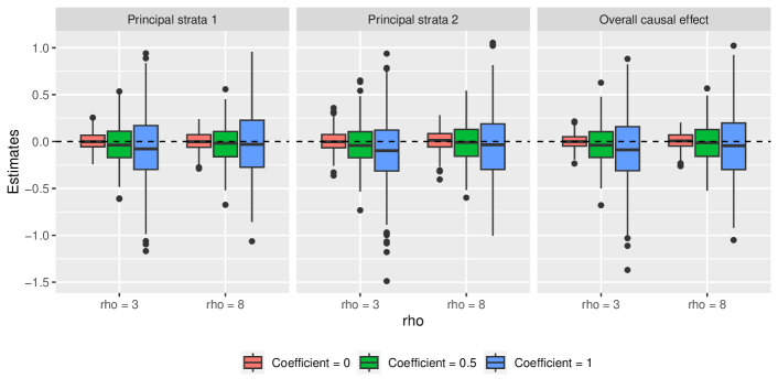
Figure 2: Distribution of point estimates minus the corresponding true values for two different principal causal effects, and the average causal effect.

First, we run a simulation with a correctly specified outcome model to investigate when the proposed approach can provide valid inference on different causal effects, and to assess the ability to estimate weakly identified parameters, such as $\rho$. Figure 2 shows box plots of posterior means minus true values for all three estimands considered across different values of $\rho$ and $c$. We obtain relatively unbiased estimators for all scenarios, though uncertainty increases as the magnitude of $c$ increases. Any bias seen here disappears in the larger sample size simulations in Appendix D. To investigate the extent to which we can learn the missing values of $S(t)$, we can examine posterior means of the full potential intermediate curve $\bm{S}$. To better visualize performance, we averaged estimates of $\bm{S}$ over all units in the sample belonging to the same cluster. This leads to three different values for each simulated data set: one for each of the three clusters. Figure 3 shows these curves across multiple data sets, where the true value is given by the dashed line. We see in the left panel of Figure 3 that when $c=0$ and there is no association between $S(t)$ and the outcome, we have very little information to impute the missing potential intermediates and therefore the three groups have similar curves. As the magnitude of $c$ grows, however, the three groups become more clearly separated as there is more information in the data to inform the missing intermediate values. Lastly, we can look at Figure 4 to see estimates of $\rho$, which dictates the correlation among the different intermediate variables. We see that when $c=0$, the estimates when the true correlation is 3 or 8 are very similar. This confirms the theoretical result in Section 4 that we have no information to learn this parameter when there is no effect of $S(t)$ on the outcome. As this effect becomes nonzero, however, we are able to estimate $\rho$ and we can see that it begins to center around the true values of 3 or 8, and the estimates are less variable as $c$ increases.

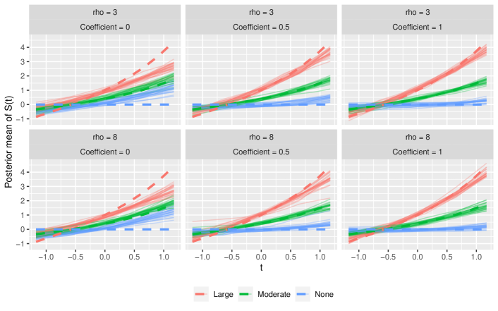
Figure 3: Estimates of $S(t)$ as a function of $t$ for each cluster of units. The dotted line corresponds to the true $\phi(t)$ for each cluster.

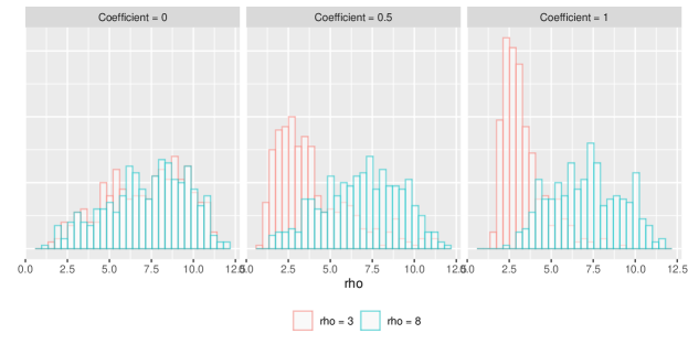
Figure 4: Distribution of point estimates for $\rho$ across all scenarios.

5.2 Model misspecification

We now utilize the same data generation procedure as before, except now we induce model misspecification by letting the true coefficients be given by $\beta(t,t^{\prime})=c(0.3+0.1t+0.1t^{2}+0.2t^{\prime}+0.15{t^{\prime}}^{2})$. We incorrectly assume that this function is linear in both $t$ and $t^{\prime}$, and therefore the manner in which we include $\bm{S}$ into the outcome model is misspecified. Figures 5 and 6 show the results from this simulation scenario. When $c=0$, there is no effect of the intermediate variable on the outcome, and therefore no model misspecification, which leads to the same unbiased results as in the previous section. When $c=0.5$, the model still performs relatively well, but when $c=1$ and there is a strong effect of the intermediate on the outcome, we obtain biased results of both principal causal effects and the overall treatment effect. Another interesting finding in Figure 6 is that the posterior distribution of $\rho$ concentrates around values of $\rho$ smaller than the true value. Not shown here are the average estimates of the intermediate values $\bm{S}$, which are less affected by the model misspecification and we obtain similar results to those seen in Figure 3.

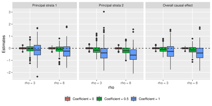
Figure 5: Distribution of point estimates minus the corresponding true values when the outcome model is misspecified.

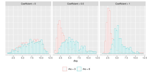
Figure 6: Distribution of point estimates for $\rho$ when the outcome model is misspecified.

6 The role of the economy on arrest rates

Understanding how the economy shapes the criminal justice system is an important question that has been studied since at least Rusche and Kirchheimer’s 1939 book “Punishment and Social Structure” (Rusche and Kirchheimer,, 1939), which posited that recessions increase coercive control because the state needs to maintain order in the face of economic crises. Empirical examinations, however, have produced mixed results, perhaps because they have not accounted for the multiple causal pathways through which the economy can impact criminal justice (Sutton,, 2004; Carmichael and Kent,, 2014). The present study examines police capacity as a potential mechanism through which economic fluctuation could impact arrest rates. Results from this study can help policymakers and criminologists situate police in their macro-economic context.

Our data consist of all cities in the United States, though we restrict attention to those with at least 50,000 people in the year 2010, since data are more reliable in larger cities. After removing observations with missing data, we have $n=596$ cities measured. The treatment variable is log gross domestic product (GDP) in 2011, which is measured in inflation-adjusted thousands of dollars, and comes from the Bureau of Economic Analysis. The intermediate variable is the number of police officers per 1000 individuals and it comes from the Law Enforcement Officers Killed and Assaulted database. The outcome is the arrest rate per 1000 people and comes from the FBI’s Uniform Crime Reports. Pre-treatment covariates consist of percent Latino, percent Black, percent with a bachelor’s degree, percent men aged 15-34, percent of vacant housing, percent foreign born, population size, and violent crime rates, all taken from the year 2010. Demographic variables come from the Census Bureau’s decennial census and American Community Survey (ACS), while violent crime rates also come from the FBI’s Uniform Crime Reports. We measure a wide range of important features of cities in order to capture confounders of the GDP, police capacity, and arrest rate relationships. Additionally, we believe that SUTVA is plausible in this study as we focused on large cities that are sufficiently separated to avoid issues with interference.

We target estimands with two different $g(\cdot)$ functions to identify different principal strata. We examine both the average potential intermediate given by $g(\bm{S})=\frac{1}{M}\sum_{t=1}^{M}S(t)$, as well as $g(\bm{S})=\text{range}(\bm{S})$. We look at principal strata defined by units with either low or high values of these two functions. Specifically, if we define $c_{m}$ and $c_{s}$ to be the sample mean and standard deviation of $S_{i}$, we look at principal strata exposure-response curves defined by $E(Y(t)\mid\overline{\bm{S}}<c_{m})$ and $E(Y(t)\mid\overline{\bm{S}}\geq c_{m})$, as well as $E(Y(t)\mid\text{range}(\bm{S})<c_{s})$ and $E(Y(t)\mid\text{range}(\bm{S})\geq c_{s})$. The first set of principal strata looks at groups of cities defined by having generally high or low values of police capacity, regardless of the shape of $\bm{S}$. The estimand depending on the range, however, looks at cities with relatively flat or steep curves for $S(t)$ as a function of $t$. Throughout, we use our proposed model with prior distributions described above. We run 10,000 MCMC chains discarding the first 2,000 as a burn-in and keeping every 8th sample.

6.1 Findings

The results of the analysis can be found in Figures 7 and 8. The coefficients for $S(t^{\prime})$ in the outcome model are given by $\beta(t,t^{\prime})=\zeta_{0}+\zeta_{1}t+\zeta_{2}t^{\prime}$, and the left panel of Figure 7 shows the posterior distribution of $(\zeta_{0},\zeta_{1},\zeta_{2})$. Police capacity tends to increase arrest rates as indicated by positive $\zeta_{0}$ values. This relationship changes with both $t$ and $t^{\prime}$, however, as the posterior distributions for $\zeta_{1}$ and $\zeta_{2}$ are away from zero. The negative values of $\zeta_{1}$ show that the effect of the potential intermediate on the outcome decreases with treatment value, while the large, positive values of $\zeta_{2}$ show that $S(t^{\prime})$ has a larger effect for larger values of $t^{\prime}$. The right panel of Figure 7 shows the impact of the economy on police capacity as measured by the values of $\phi(t)$. A large number (96%) of cities are estimated to have no impact of the economy on policy capacity (constant $\phi(t)$), while a few cities have moderate to large impacts. This also highlights the clustering done by the Dirichlet process, as we see distinct clusters with different shapes of $\phi(t)$. Additionally, the 95% credible interval for $\rho$ is (6.54, 12.87) indicating a strong degree of correlation across $S(t)$ values.

Figure 8 shows the principal strata exposure-response curves for all four of the principal strata examined. Looking at the left panel, we can see that cities with higher average values of potential police capacity have higher arrest rates than those with low police capacity, however, this difference becomes smaller under larger values of GDP. This indicates that cities with high police capacity see large reductions in arrest rates as the economy improves, while cities with low police capacity see relatively little benefit of the economy on reducing arrest rates. Looking at principal strata defined by $\text{range}(\bm{S})$, we see that the associative and dissociative effects are very similar to each other. The effect of GDP on arrests within the strata of cities where there is an effect of GDP on police capacity (high $\text{range}(\bm{S})$) is similar to the effect in strata with no effect of GDP on police capacity (low $\text{range}(\bm{S})$). This, coupled with the fact that 96% of cities had flat $\phi(t)$ functions, shows that police capacity does not appear to mediate the relationship between GDP and arrest rates.

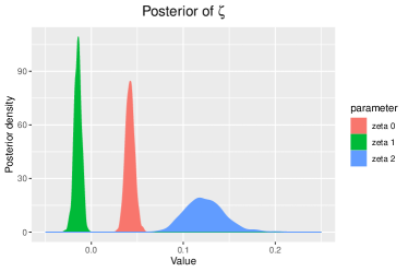
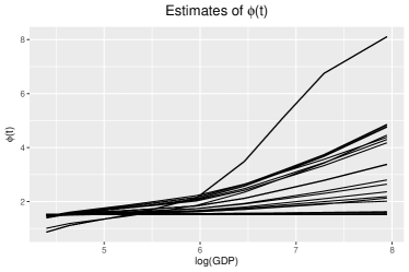
Figure 7: The left panel shows the posterior distributions of $(\zeta_{0},\zeta_{1},\zeta_{2})$, and the right panel shows the posterior mean of $\phi_{i}(t)$ for all $i=1,\dots,n$.

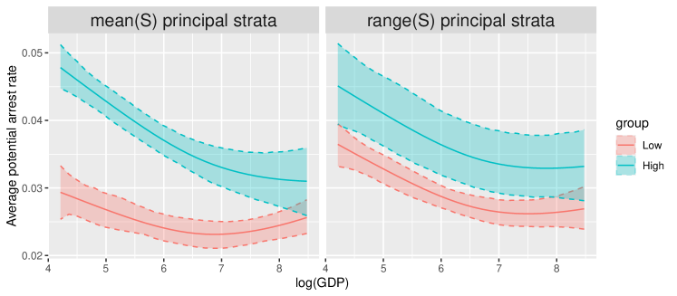
Figure 8: The left panel shows estimates and pointwise 95% credible intervals for $E(Y(t)\mid\overline{\bm{S}}<c_{m})$ and $E(Y(t)\mid\overline{\bm{S}}\geq c_{m})$. The right panel shows the corresponding quantities for $E(Y(t)\mid\text{range}(\bm{S})<c_{s})$ and $E(Y(t)\mid\text{range}(\bm{S})\geq c_{s})$.

7 Discussion

This manuscript developed methodology to estimate principal causal effects when both the treatment and intermediate variables are continuous. We formalized assumptions and estimands in this setting, and provided a flexible, nonparametric Bayesian model to estimate all estimands of interest. One key feature of the manuscript is that we provide theoretical justification for the use of the outcome model to learn the correlation between the potential intermediate values, which is a crucial parameter, and has implications in simpler settings with binary treatments and binary intermediates as well. Our nonparametric Bayesian formulation also clusters units based on their treatment-intermediate association, which naturally clusters units into different principal strata of interest. Lastly, we analyzed the relationships between GDP, police capacity, and arrest rates to provide an improved understanding of the relationship between the economy and arrest rates.

While our model utilizes a flexible, nonparametric Bayesian model for the treatment-intermediate association, our approach is reliant on a relatively well-specified outcome model, both for estimation of causal effects and for learning the correlation between the intermediate variables. Future work could extend our methodology to more flexible outcome modeling strategies. This would complicate the updating of the unknown potential intermediate values and the correlation between them, though would have the potential to reduce the negative impacts of model misspecification. As a sensitivity analysis to model specification, one can estimate the proposed model to estimate an overall exposure-response curve $E(Y(t))$, as well as a more flexible (semiparametric) model that does not include the $\bm{S}$ values to estimate $E(Y(t))$. Large differences between these two estimates would provide evidence of model misspecification with respect to how the $\bm{S}$ values are included in the outcome model. Additionally, sensitivity analysis to violations of the unconfoundedness assumption could be incorporated to assess the robustness of findings to unmeasured confounding (Franks et al.,, 2020), though we leave this extension to future work.

Appendix A Identification of causal estimands

Throughout this section we focus on estimands of the form $E[Y(t)\mid a<g(\bm{S})<b]$ for some function $g(\cdot)$, though analogous calculations would apply for other estimands. First we can see that

$$E[Y(t)\mid a<g(\bm{S})<b] =E_{\bm{X}|a<g(\bm{S})<b}E[Y(t)\mid a<g(\bm{S})<b,\bm{X}]$$

$$=E_{\bm{X}|a<g(\bm{S})<b}E[Y(t)\mid T=t,a<g(\bm{S})<b,\bm{X}]$$

$$=E_{\bm{X}|a<g(\bm{S})<b}E[Y\mid T=t,a<g(\bm{S})<b,\bm{X}].$$

The first equality relied on rules of iterated expectations, while the second and third lines utilized the no unmeasured confounding and SUTVA assumptions, respectively. The outer expectation is relatively easy to work with, so we focus on the inner expectation now, which is slightly more complex since we are conditioning on $\bm{S}$ satisfying a constraint, rather than being set to a fixed value that we can plug into the outcome regression equation. This inner expectation can be decomposed as

$$E[Y\mid T=t,a<g(\bm{S})<b,\bm{X}] =E_{S\mid T,\bm{X},a<g(\bm{S})<b}E[Y\mid T=t,a<g(\bm{S})<b,\bm{X},\bm{S}=\bm{s}]$$

$$=E_{S\mid T,\bm{X},a<g(\bm{S})<b}E[Y\mid T=t,\bm{X},\bm{S}=\bm{s}]$$

The inner of these two expectations is straightforward to calculate since we have an outcome model for $E[Y\mid T=t,\bm{X},\bm{S}=\bm{s}]$. We simply need to be able to average this outcome model with respect to the distribution of $\bm{S}\mid T=t,\bm{X}=\bm{x},a<g(\bm{S})<b$. This density can be written as

$$f(\bm{s}\mid T=t,\bm{X}=\bm{x},a<g(\bm{S})<b) =\frac{f(\bm{s}\mid T=t,\bm{X}=\bm{x})P(a<g(\bm{S})<b|T=t,\bm{X}=\bm{x},\bm{S}=\bm{s})}{P(a<g(\bm{S})<b|T=t,\bm{X}=\bm{x})}$$

$$=\frac{f(\bm{s}\mid T=t,\bm{X}=\bm{x})1(a<g(\bm{s})<b)}{P(a<g(\bm{S})<b|T=t,\bm{X}=\bm{x})}$$

Both the numerator and the denominator can be calculated from the model for $\bm{S}\mid T,X$. The denominator can be calculated empirically by sampling a large number of times from $\bm{S}\mid T,X$ and calculating the proportion of draws for which the inequality is true. In practice, we will calculate $E[Y\mid T=t,a<g(\bm{S})<b,\bm{X}]$ by sampling draws of $\bm{S}$ from the distribution of $\bm{S}|T,X$, calculating $E[Y\mid T=t,\bm{S}=\bm{s},X]$ for each draw, and taking a weighted average of these values with weights given by $\frac{1(a<g(\bm{s})<b)}{P(a<g(\bm{S})<b|T=t,\bm{X}=\bm{x})}.$ Combining all of these steps, we can see that

$$E(Y(t)\mid a<g(\bm{S})<b)$$

$$= E_{\bm{X}|a<g(\bm{S})<b}\Big{[}E(Y\mid T=t,a<g(\bm{S})<b,\bm{X})\Big{]}$$

$$= E_{\bm{X}|a<g(\bm{S})<b}\bigg{\{}E_{S\mid T,\bm{X},a<g(\bm{S})<b}\Big{[}E(Y\mid T=t,\bm{X},\bm{S}=\bm{s})\Big{]}\bigg{\}}$$

$$= E_{\bm{X}|a<g(\bm{S})<b}\bigg{\{}\int_{\bm{s}}E(Y\mid T=t,\bm{X},\bm{S}=\bm{s})f(\bm{s}\mid T=t,\bm{X}=\bm{x},a<g(\bm{S})<b)d\bm{s}\bigg{\}}$$

$$= E_{\bm{X}|a<g(\bm{S})<b}\bigg{\{}\int_{\bm{s}}E(Y\mid T=t,\bm{X},\bm{S}=\bm{s})\frac{f(\bm{s}\mid T=t,\bm{X}=\bm{x})1(a<g(\bm{s})<b)}{P(a<g(\bm{S})<b|T=t,\bm{X}=\bm{x})}d\bm{s}\bigg{\}}$$

$$= \int_{\bm{x}}\int_{\bm{s}}E(Y\mid T=t,\bm{X},\bm{S}=\bm{s})\frac{f(\bm{s}\mid T=t,\bm{X}=\bm{x})1(a<g(\bm{s})<b)}{P(a<g(\bm{S})<b|T=t,\bm{X}=\bm{x})}d\bm{s}\ dF_{\bm{X}\mid a<g(\bm{S})<b}(\bm{x}),$$

and we get the final expression seen in the manuscript.

Appendix B Proof of results on correlation parameter

In this section, we provide technical details for the derivation of the marginal posterior of $\rho$, as well as a proof of the fact that this posterior is maximized at the true correlation parameter.

B.1 Deriving marginal posterior of $\rho$

Utilizing the notation that the potential intermediates are given by $\bm{S}_{i}(t)=\bm{S}_{i}$, and the observed intermediate is $S_{i}$, the marginal posterior distribution can be written as

$$P(\rho|\mathcal{D}) \propto P(\rho)\prod_{i=1}^{n}\Bigg{\{}P\Big{(}Y_{i}|T_{i},\bm{X}_{i},\bm{S},\rho\Big{)}P\Big{(}\bm{S}_{i}|T_{i},S_{i},\bm{X}_{i},\rho\Big{)}\Bigg{\}}$$

$$\propto P(\rho)\Bigg{\{}\prod_{i=1}^{n}|\widetilde{\bm{\Sigma}}_{si}|^{-1/2}\Bigg{\}}\ \text{exp}\Bigg{\{}-\frac{\sum_{i=1}^{n}(\widetilde{Y}_{i}-\bm{S}_{i}^{T}\bm{\beta}_{i})^{2}}{2\sigma^{2}}\Bigg{\}}$$

$$\times\ \text{exp}\Bigg{\{}-\frac{1}{2}\sum_{i=1}^{n}(\bm{S}_{i}-\widetilde{\bm{\mu}}_{si})^{T}\widetilde{\bm{\Sigma}}_{si}^{-1}(\bm{S}_{i}-\widetilde{\bm{\mu}}_{si})\Bigg{\}}$$

$$\propto P(\rho)\Bigg{\{}\prod_{i=1}^{n}|\widetilde{\bm{\Sigma}}_{si}|^{-1/2}\Bigg{\}}$$

$$\times\text{exp}\Bigg{\{}-\frac{1}{2}\sum_{i=1}^{n}-2\bm{S}_{i}^{T}\bigg{(}\frac{\widetilde{Y}_{i}\bm{\beta}_{i}}{\sigma^{2}}+\widetilde{\bm{\Sigma}}_{si}^{-1}\widetilde{\bm{\mu}}_{si}\bigg{)}+\bm{S}_{i}^{T}\bigg{(}\frac{\bm{\beta}_{i}\bm{\beta}_{i}^{T}}{\sigma^{2}}+\widetilde{\bm{\Sigma}}_{si}^{-1}\bigg{)}\bm{S}_{i}+\widetilde{\bm{\mu}}_{si}^{T}\widetilde{\bm{\Sigma}}_{si}\widetilde{\bm{\mu}}_{si}\Bigg{\}}$$

The left two terms in the exponential represent the kernel of a multivariate normal distribution for $\bm{S}_{i}$ with mean given by

$$\bm{M}=\bigg{(}\frac{\bm{\beta}_{i}\bm{\beta}_{i}^{T}}{\sigma^{2}}+\widetilde{\bm{\Sigma}}_{si}^{-1}\bigg{)}^{-1}\bigg{(}\frac{\widetilde{Y}_{i}\bm{\beta}_{i}}{\sigma^{2}}+\widetilde{\bm{\Sigma}}_{si}^{-1}\widetilde{\bm{\mu}}_{si}\bigg{)}$$

and variance given by

$$\bm{V}=\bigg{(}\frac{\bm{\beta}_{i}\bm{\beta}_{i}^{T}}{\sigma^{2}}+\widetilde{\bm{\Sigma}}_{si}^{-1}\bigg{)}^{-1}.$$

With that in mind, we can multiply and divide this expression by the determinant term of the corresponding multivariate normal distribution, as well as adding and subtracting the relevant constants into the exponential term to get the full multivariate normal density with this mean and variance. The determinant term that we will multiply and divide by is given by

$$\Bigg{\{}\prod_{i=1}^{n}\bigg{|}\bigg{(}\frac{\bm{\beta}_{i}\bm{\beta}_{i}^{T}}{\sigma^{2}}+\widetilde{\bm{\Sigma}}_{si}^{-1}\bigg{)}^{-1}\bigg{|}^{-1/2}\Bigg{\}} =\Bigg{\{}\prod_{i=1}^{n}\bigg{|}\bigg{(}\frac{\bm{\beta}_{i}\bm{\beta}_{i}^{T}}{\sigma^{2}}+\widetilde{\bm{\Sigma}}_{si}^{-1}\bigg{)}\bigg{|}^{1/2}\Bigg{\}}.$$

The constant term that we will add and subtract to the exponential term of this posterior distribution is given by

$$\bigg{(}\frac{\widetilde{Y}_{i}\bm{\beta}_{i}}{\sigma^{2}}+\widetilde{\bm{\Sigma}}_{si}^{-1}\widetilde{\bm{\mu}}_{si}\bigg{)}^{T}\bigg{(}\frac{\bm{\beta}_{i}\bm{\beta}_{i}^{T}}{\sigma^{2}}+\widetilde{\bm{\Sigma}}_{si}^{-1}\bigg{)}^{-1}\bigg{(}\frac{\widetilde{Y}_{i}\bm{\beta}_{i}}{\sigma^{2}}+\widetilde{\bm{\Sigma}}_{si}^{-1}\widetilde{\bm{\mu}}_{si}\bigg{)}.$$

After the inclusion of these terms, we are left with

$$P(\rho)\left\{\prod_{i=1}^{n}\frac{|\widetilde{\bm{\Sigma}}_{si}^{-1}|^{1/2}}{\Bigg{|}\bigg{(}\frac{\bm{\beta}_{i}\bm{\beta}_{i}^{T}}{\sigma^{2}}+\widetilde{\bm{\Sigma}}_{si}^{-1}\bigg{)}\Bigg{|}^{1/2}}\right\}$$

$$\times\ \text{exp}\Bigg{\{}-\frac{1}{2}\Bigg{[}\widetilde{\bm{\mu}}_{si}^{T}\widetilde{\bm{\Sigma}}_{si}\widetilde{\bm{\mu}}_{si}-\bigg{(}\frac{\widetilde{Y}_{i}\bm{\beta}_{i}}{\sigma^{2}}+\widetilde{\bm{\Sigma}}_{si}^{-1}\widetilde{\bm{\mu}}_{si}\bigg{)}^{T}\bigg{(}\frac{\bm{\beta}_{i}\bm{\beta}_{i}^{T}}{\sigma^{2}}+\widetilde{\bm{\Sigma}}_{si}^{-1}\bigg{)}^{-1}\bigg{(}\frac{\widetilde{Y}_{i}\bm{\beta}_{i}}{\sigma^{2}}+\widetilde{\bm{\Sigma}}_{si}^{-1}\widetilde{\bm{\mu}}_{si}\bigg{)}\Bigg{]}\Bigg{\}}$$

$$\times\ \prod_{i=1}^{n}f(\bm{S}_{i};\bm{M},\bm{V})$$

where $f(\bm{S}_{i};\bm{M},\bm{V})$ represents the density of a normal distribution with mean $\bm{M}$ and variance $\bm{V}$ evaluated at $\bm{S}_{i}$. Only the final term contains $\bm{S}_{i}$ and it is a density function, so if we integrate this expression with respect to $\bm{S}_{i}$, the final term integrates to 1 and we are left with the remaining terms. To obtain the final desired result, we can use a result on determinants of matrices that are the sum of a positive definite and a rank 1 matrix to see that

$$\Bigg{|}\bigg{(}\frac{\bm{\beta}_{i}\bm{\beta}_{i}^{T}}{\sigma^{2}}+\widetilde{\bm{\Sigma}}_{si}^{-1}\bigg{)}\Bigg{|}=|\widetilde{\bm{\Sigma}}_{si}^{-1}|\bigg{(}1+\frac{\bm{\beta}_{i}^{T}\widetilde{\bm{\Sigma}}_{si}\bm{\beta}_{i}}{\sigma^{2}}\bigg{)}$$

and therefore we have that

$$\left\{\prod_{i=1}^{n}\frac{|\widetilde{\bm{\Sigma}}_{si}^{-1}|^{1/2}}{\Bigg{|}\bigg{(}\frac{\bm{\beta}_{i}\bm{\beta}_{i}^{T}}{\sigma^{2}}+\widetilde{\bm{\Sigma}}_{si}^{-1}\bigg{)}\Bigg{|}^{1/2}}\right\} =\left\{\prod_{i=1}^{n}\frac{|\widetilde{\bm{\Sigma}}_{si}^{-1}|^{1/2}}{\Bigg{(}|\widetilde{\bm{\Sigma}}_{si}^{-1}|\bigg{(}1+\frac{\bm{\beta}_{i}^{T}\widetilde{\bm{\Sigma}}_{si}\bm{\beta}_{i}}{\sigma^{2}}\bigg{)}\Bigg{)}^{1/2}}\right\}$$

$$=\prod_{i=1}^{n}\bigg{(}1+\frac{\bm{\beta}_{i}^{T}\widetilde{\bm{\Sigma}}_{si}\bm{\beta}_{i}}{\sigma^{2}}\bigg{)}^{-1/2}$$

Combining this, with the results from above, we can see that the marginal posterior becomes

$$P(\rho)\left\{\prod_{i=1}^{n}\bigg{(}1+\frac{\bm{\beta}_{i}^{T}\widetilde{\bm{\Sigma}}_{si}\bm{\beta}_{i}}{\sigma^{2}}\bigg{)}^{-1/2}\right\}$$

$$\times\ \text{exp}\Bigg{\{}-\frac{1}{2}\Bigg{[}\widetilde{\bm{\mu}}_{si}^{T}\widetilde{\bm{\Sigma}}_{si}\widetilde{\bm{\mu}}_{si}-\bigg{(}\frac{\widetilde{Y}_{i}\bm{\beta}_{i}}{\sigma^{2}}+\widetilde{\bm{\Sigma}}_{si}^{-1}\widetilde{\bm{\mu}}_{si}\bigg{)}^{T}\bigg{(}\frac{\bm{\beta}_{i}\bm{\beta}_{i}^{T}}{\sigma^{2}}+\widetilde{\bm{\Sigma}}_{si}^{-1}\bigg{)}^{-1}\bigg{(}\frac{\widetilde{Y}_{i}\bm{\beta}_{i}}{\sigma^{2}}+\widetilde{\bm{\Sigma}}_{si}^{-1}\widetilde{\bm{\mu}}_{si}\bigg{)}\Bigg{]}\Bigg{\}}$$

B.2 Posterior mode of $\rho$

To help simplify expressions, we need to use a result on the inverse of the sum of a positive definite matrix and a rank 1 matrix that gives the following:

$$\bigg{(}\frac{\bm{\beta}_{i}\bm{\beta}_{i}^{T}}{\sigma^{2}}+\widetilde{\bm{\Sigma}}_{si}^{-1}\bigg{)}^{-1} =\widetilde{\bm{\Sigma}}_{si}-\frac{\widetilde{\bm{\Sigma}}_{si}\bm{\beta}_{i}\bm{\beta}_{i}^{T}\widetilde{\bm{\Sigma}}_{si}}{1+Tr(\bm{\beta}_{i}\bm{\beta}_{i}^{T}\widetilde{\bm{\Sigma}}_{si})}$$

$$=\widetilde{\bm{\Sigma}}_{si}-\frac{\widetilde{\bm{\Sigma}}_{si}\bm{\beta}_{i}\bm{\beta}_{i}^{T}\widetilde{\bm{\Sigma}}_{si}}{\sigma^{2}\bigg{(}1+Tr\Big{(}\frac{\bm{\beta}_{i}\bm{\beta}_{i}^{T}\widetilde{\bm{\Sigma}}_{si}}{\sigma^{2}}\Big{)}\bigg{)}}$$

$$=\widetilde{\bm{\Sigma}}_{si}-\frac{\widetilde{\bm{\Sigma}}_{si}\bm{\beta}_{i}\bm{\beta}_{i}^{T}\widetilde{\bm{\Sigma}}_{si}}{\sigma^{2}+\bm{\beta}_{i}^{T}\widetilde{\bm{\Sigma}}_{si}\bm{\beta}_{i}}$$

Now that we have this we can aim to show what value maximizes the marginal posterior of $\rho$. For simplicity of calculations, and without loss of generality, we assume that $\sigma^{2}=1$. For these calculations we also assume a flat, improper prior $P(\rho)\propto 1$. This is to highlight what value of $\rho$ is implied from the outcome model specification above without any influence from the prior. We expect a standard prior distribution would lead to a posterior mode that is a weighted average of the mode we derive here and the prior mode with weights dictated by the sample size and the prior variance. Additionally, the result presented here is asymptotic and therefore any influence from the prior will be negligible in large samples. Lastly, we examine $\log[P(\rho|\mathcal{D})]$ as it will simplify calculations and the calculation of derivatives. First, we can re-arrange the log posterior as

$$\log[P(\rho|\mathcal{D})] =-\frac{1}{2}\sum_{i=1}^{n}\Bigg{\{}\log(1+\bm{\beta}_{i}^{T}\widetilde{\bm{\Sigma}}_{si}\bm{\beta}_{i})+\widetilde{\bm{\mu}}_{si}^{T}\widetilde{\bm{\Sigma}}_{si}\widetilde{\bm{\mu}}_{si}$$

$$-\bigg{(}\widetilde{Y}_{i}\bm{\beta}_{i}+\widetilde{\bm{\Sigma}}_{si}^{-1}\widetilde{\bm{\mu}}_{si}\bigg{)}^{T}\bigg{(}\bm{\beta}_{i}\bm{\beta}_{i}^{T}+\widetilde{\bm{\Sigma}}_{si}^{-1}\bigg{)}^{-1}\bigg{(}\widetilde{Y}_{i}\bm{\beta}_{i}+\widetilde{\bm{\Sigma}}_{si}^{-1}\widetilde{\bm{\mu}}_{si}\bigg{)}\Bigg{\}}$$

$$=-\frac{1}{2}\sum_{i=1}^{n}\Bigg{\{}\log(1+\bm{\beta}_{i}^{T}\widetilde{\bm{\Sigma}}_{si}\bm{\beta}_{i})+\widetilde{\bm{\mu}}_{si}^{T}\widetilde{\bm{\Sigma}}_{si}\widetilde{\bm{\mu}}_{si}$$

$$-\bigg{(}\widetilde{Y}_{i}\bm{\beta}_{i}+\widetilde{\bm{\Sigma}}_{si}^{-1}\widetilde{\bm{\mu}}_{si}\bigg{)}^{T}\bigg{(}\widetilde{\bm{\Sigma}}_{si}-\frac{\widetilde{\bm{\Sigma}}_{si}\bm{\beta}_{i}\bm{\beta}_{i}^{T}\widetilde{\bm{\Sigma}}_{si}}{1+\bm{\beta}_{i}^{T}\widetilde{\bm{\Sigma}}_{si}\bm{\beta}_{i}}\bigg{)}\bigg{(}\widetilde{Y}_{i}\bm{\beta}_{i}+\widetilde{\bm{\Sigma}}_{si}^{-1}\widetilde{\bm{\mu}}_{si}\bigg{)}\Bigg{\}}$$

$$=-\frac{1}{2}\sum_{i=1}^{n}\Bigg{\{}\log(1+\bm{\beta}_{i}^{T}\widetilde{\bm{\Sigma}}_{si}\bm{\beta}_{i})-\widetilde{Y}_{i}^{2}\bm{\beta}_{i}^{T}\widetilde{\bm{\Sigma}}_{si}\bm{\beta}_{i}-2\widetilde{Y}_{i}\widetilde{\bm{\mu}}_{si}^{T}\bm{\beta}_{i}$$

$$+\frac{\widetilde{Y}_{i}^{2}\bm{\beta}_{i}^{T}\widetilde{\bm{\Sigma}}_{si}\bm{\beta}_{i}\bm{\beta}_{i}^{T}\widetilde{\bm{\Sigma}}_{si}\bm{\beta}_{i}+2\widetilde{Y}_{i}\bm{\beta}_{i}^{T}\widetilde{\bm{\Sigma}}_{si}\bm{\beta}_{i}\bm{\beta}_{i}^{T}\widetilde{\bm{\mu}}_{si}+\widetilde{\bm{\mu}}_{si}^{T}\bm{\beta}_{i}\bm{\beta}_{i}^{T}\widetilde{\bm{\mu}}_{si}}{1+\bm{\beta}_{i}^{T}\widetilde{\bm{\Sigma}}_{si}\bm{\beta}_{i}}\Bigg{\}}$$

$$=-\frac{1}{2}\sum_{i=1}^{n}\left\{\log(1+\bm{\beta}_{i}^{T}\widetilde{\bm{\Sigma}}_{si}\bm{\beta}_{i})-\frac{\Big{(}\widetilde{Y}_{i}^{2}\bm{\beta}_{i}^{T}\widetilde{\bm{\Sigma}}_{si}\bm{\beta}_{i}+2\widetilde{Y}_{i}\widetilde{\bm{\mu}}_{si}^{T}\bm{\beta}_{i}-\widetilde{\bm{\mu}}_{si}^{T}\bm{\beta}_{i}\bm{\beta}_{i}^{T}\widetilde{\bm{\mu}}_{si}\Big{)}}{1+\bm{\beta}_{i}^{T}\widetilde{\bm{\Sigma}}_{si}\bm{\beta}_{i}}\right\}$$

We can now take the derivative of this with respect to $\rho$, where it is important to remember throughout that both $\widetilde{\bm{\mu}}_{si}$ and $\widetilde{\bm{\Sigma}}_{si}$ are functions of $\rho$.

$$\frac{d\log[P(\rho|\mathcal{D})]}{d\rho} =-\frac{1}{2}\sum_{i=1}^{n}\Bigg{\{}\frac{\frac{d(\bm{\beta}_{i}^{T}\widetilde{\bm{\Sigma}}_{si}\bm{\beta}_{i})}{d\rho}}{1+\bm{\beta}_{i}^{T}\widetilde{\bm{\Sigma}}_{si}\bm{\beta}_{i}}+\frac{(1+\bm{\beta}_{i}^{T}\widetilde{\bm{\Sigma}}_{si}\bm{\beta}_{i})\Big{(}-\widetilde{Y}_{i}^{2}\frac{d(\bm{\beta}_{i}^{T}\widetilde{\bm{\Sigma}}_{si}\bm{\beta}_{i})}{d\rho}-2\widetilde{Y}_{i}\frac{d(\widetilde{\bm{\mu}}_{si}^{T}\bm{\beta}_{i})}{d\rho}+\frac{d(\widetilde{\bm{\mu}}_{si}^{T}\bm{\beta}_{i}\bm{\beta}_{i}^{T}\widetilde{\bm{\mu}}_{si})}{d\rho}\Big{)}}{(1+\bm{\beta}_{i}^{T}\widetilde{\bm{\Sigma}}_{si}\bm{\beta}_{i})^{2}}$$

$$-\frac{\frac{d(\bm{\beta}_{i}^{T}\widetilde{\bm{\Sigma}}_{si}\bm{\beta}_{i})}{d\rho}\Big{(}-\widetilde{Y}_{i}^{2}\bm{\beta}_{i}^{T}\widetilde{\bm{\Sigma}}_{si}\bm{\beta}_{i}-2\widetilde{Y}_{i}\widetilde{\bm{\mu}}_{si}^{T}\bm{\beta}_{i}+\widetilde{\bm{\mu}}_{si}^{T}\bm{\beta}_{i}\bm{\beta}_{i}^{T}\widetilde{\bm{\mu}}_{si}\Big{)}}{(1+\bm{\beta}_{i}^{T}\widetilde{\bm{\Sigma}}_{si}\bm{\beta}_{i})^{2}}\Bigg{\}}$$

$$=-\frac{1}{2}\sum_{i=1}^{n}\Bigg{\{}\frac{\frac{d(\bm{\beta}_{i}^{T}\widetilde{\bm{\Sigma}}_{si}\bm{\beta}_{i})}{d\rho}}{1+\bm{\beta}_{i}^{T}\widetilde{\bm{\Sigma}}_{si}\bm{\beta}_{i}}+\frac{(1+\bm{\beta}_{i}^{T}\widetilde{\bm{\Sigma}}_{si}\bm{\beta}_{i})\Big{(}-\widetilde{Y}_{i}^{2}\frac{d(\bm{\beta}_{i}^{T}\widetilde{\bm{\Sigma}}_{si}\bm{\beta}_{i})}{d\rho}-2\widetilde{Y}_{i}\frac{d(\widetilde{\bm{\mu}}_{si}^{T}\bm{\beta}_{i})}{d\rho}+2\widetilde{\bm{\mu}}_{si}^{T}\bm{\beta}_{i}\frac{d(\widetilde{\bm{\mu}}_{si}^{T}\bm{\beta}_{i})}{d\rho}\Big{)}}{(1+\bm{\beta}_{i}^{T}\widetilde{\bm{\Sigma}}_{si}\bm{\beta}_{i})^{2}}$$

$$-\frac{\frac{d(\bm{\beta}_{i}^{T}\widetilde{\bm{\Sigma}}_{si}\bm{\beta}_{i})}{d\rho}\Big{(}-\widetilde{Y}_{i}^{2}\bm{\beta}_{i}^{T}\widetilde{\bm{\Sigma}}_{si}\bm{\beta}_{i}-2\widetilde{Y}_{i}\widetilde{\bm{\mu}}_{si}^{T}\bm{\beta}_{i}+\widetilde{\bm{\mu}}_{si}^{T}\bm{\beta}_{i}\bm{\beta}_{i}^{T}\widetilde{\bm{\mu}}_{si}\Big{)}}{(1+\bm{\beta}_{i}^{T}\widetilde{\bm{\Sigma}}_{si}\bm{\beta}_{i})^{2}}\Bigg{\}}$$

$$=-\frac{1}{2}\sum_{i=1}^{n}\Bigg{\{}\frac{\frac{d(\bm{\beta}_{i}^{T}\widetilde{\bm{\Sigma}}_{si}\bm{\beta}_{i})}{d\rho}\Big{(}1+\bm{\beta}_{i}^{T}\widetilde{\bm{\Sigma}}_{si}\bm{\beta}_{i}-\widetilde{Y}_{i}^{2}+2\widetilde{Y}_{i}\widetilde{\bm{\mu}}_{si}^{T}\bm{\beta}_{i}-\widetilde{\bm{\mu}}_{si}^{T}\bm{\beta}_{i}\bm{\beta}_{i}^{T}\widetilde{\bm{\mu}}_{si}\Big{)}}{(1+\bm{\beta}_{i}^{T}\widetilde{\bm{\Sigma}}_{si}\bm{\beta}_{i})^{2}}$$

$$+\frac{\frac{d(\widetilde{\bm{\mu}}_{si}^{T}\bm{\beta}_{i})}{d\rho}\Big{(}-2\widetilde{Y}_{i}-2\widetilde{Y}_{i}\bm{\beta}_{i}^{T}\widetilde{\bm{\Sigma}}_{si}\bm{\beta}_{i}+2\widetilde{\bm{\mu}}_{si}^{T}\bm{\beta}_{i}+2\widetilde{\bm{\mu}}_{si}^{T}\bm{\beta}_{i}\bm{\beta}_{i}^{T}\widetilde{\bm{\Sigma}}_{si}\bm{\beta}_{i}\Big{)}}{(1+\bm{\beta}_{i}^{T}\widetilde{\bm{\Sigma}}_{si}\bm{\beta}_{i})^{2}}\Bigg{\}}$$

Our goal is to find the value of $\rho$ for which the above expression equals zero. Therefore, we need to find the value of $\rho$ such that the following is true:

$$\frac{1}{2}\sum_{i=1}^{n}\left\{\frac{\frac{d(\bm{\beta}_{i}^{T}\widetilde{\bm{\Sigma}}_{si}\bm{\beta}_{i})}{d\rho}\bigg{(}1+\bm{\beta}_{i}^{T}\widetilde{\bm{\Sigma}}_{si}\bm{\beta}_{i}-\widetilde{\bm{\mu}}_{si}^{T}\bm{\beta}_{i}\bm{\beta}_{i}^{T}\widetilde{\bm{\mu}}_{si}\bigg{)}+2\frac{d(\widetilde{\bm{\mu}}_{si}^{T}\bm{\beta}_{i})}{d\rho}\bigg{(}\widetilde{\bm{\mu}}_{si}^{T}\bm{\beta}_{i}+\widetilde{\bm{\mu}}_{si}^{T}\bm{\beta}_{i}\bm{\beta}_{i}^{T}\widetilde{\bm{\Sigma}}_{si}\bm{\beta}_{i}\bigg{)}}{(1+\bm{\beta}_{i}^{T}\widetilde{\bm{\Sigma}}_{si}\bm{\beta}_{i}))^{2}}\right\}$$

$$= \ -\frac{1}{2}\sum_{i=1}^{n}\left\{\frac{\frac{d(\bm{\beta}_{i}^{T}\widetilde{\bm{\Sigma}}_{si}\bm{\beta}_{i})}{d\rho}\bigg{(}2\widetilde{Y}_{i}\widetilde{\bm{\mu}}_{si}^{T}\bm{\beta}_{i}-\widetilde{Y}_{i}^{2}\bigg{)}+\frac{d(\widetilde{\bm{\mu}}_{si}^{T}\bm{\beta}_{i})}{d\rho}\bigg{(}-2\widetilde{Y}_{i}-2\widetilde{Y}_{i}\bm{\beta}_{i}^{T}\widetilde{\bm{\Sigma}}_{si}\bm{\beta}_{i}\bigg{)}}{(1+\bm{\beta}_{i}^{T}\widetilde{\bm{\Sigma}}_{si}\bm{\beta}_{i})^{2}}\right\}$$ (2)

There are a couple of important facts about $\widetilde{Y}_{i}$ that will be useful here. The first is that we can write $\widetilde{Y}_{i}=\bm{S}_{i}\bm{\beta}_{i}+\epsilon_{i}$. This implies that the conditional expectation of $\widetilde{Y}_{i}$ given $S_{i}$ is $\widetilde{\bm{\mu}}_{si}^{T}(\rho^{*})\bm{\beta}_{i}$, where we have defined $\widetilde{\bm{\mu}}_{si}^{T}(\rho^{*})$ to be the value of $\widetilde{\bm{\mu}}_{si}^{T}$ at the true correlation parameter. Additionally, the conditional variance of $\widetilde{Y}_{i}$ is equal to $1+\bm{\beta}_{i}^{T}\widetilde{\bm{\Sigma}}_{si}(\rho)\bm{\beta}_{i}$, where $\widetilde{\bm{\Sigma}}_{si}(\rho^{*})$ is the value of $\widetilde{\bm{\Sigma}}_{si}$ at the true correlation parameter. We can also write $\bm{S}_{i}=\widetilde{\bm{\mu}}_{si}^{T}(\rho^{*})+\bm{\eta}_{i}$ where $\text{Var}(\bm{\eta}_{i})=\widetilde{\bm{\Sigma}}_{si}(\rho^{*})$. Both $\bm{\eta}_{i}$ and $\epsilon_{i}$ are independent across observations and of all other random variables. Putting all this together, we can write $\widetilde{Y}_{i}=\widetilde{\bm{\mu}}_{si}^{T}(\rho^{*})\bm{\beta}_{i}+\bm{\eta}_{i}^{T}\bm{\beta}_{i}+\epsilon_{i}$ or alternatively, we can write $\widetilde{Y}_{i}=\widetilde{\bm{\mu}}_{si}^{T}(\rho^{*})\bm{\beta}_{i}+\epsilon_{i}^{\prime}$, where $\text{Var}(\epsilon_{i}^{\prime})=1+\bm{\beta}_{i}^{T}\widetilde{\bm{\Sigma}}_{si}(\rho)\bm{\beta}_{i}$. Using this, we can express the right hand side of equation (2) as

$$-\frac{1}{2}\sum_{i=1}^{n}\Bigg{\{}\frac{\frac{d(\bm{\beta}_{i}^{T}\widetilde{\bm{\Sigma}}_{si}\bm{\beta}_{i})}{d\rho}\bigg{(}2\widetilde{\bm{\mu}}_{si}^{T}(\rho^{*})\bm{\beta}_{i}\bm{\beta}_{i}^{T}\widetilde{\bm{\mu}}_{si}+2\epsilon_{i}^{\prime}\widetilde{\bm{\mu}}_{si}^{T}\bm{\beta}_{i}-\widetilde{\bm{\mu}}_{si}^{T}(\rho^{*})\bm{\beta}_{i}\bm{\beta}_{i}^{T}\widetilde{\bm{\mu}}_{si}(\rho^{*})-2\epsilon_{i}^{\prime}\widetilde{\bm{\mu}}_{si}^{T}(\rho^{*})\bm{\beta}_{i}-{\epsilon_{i}^{\prime}}^{2}\bigg{)}}{(1+\bm{\beta}_{i}^{T}\widetilde{\bm{\Sigma}}_{si}\bm{\beta}_{i})^{2}}$$

$$\ \ +\frac{\frac{d(\widetilde{\bm{\mu}}_{si}^{T}\bm{\beta}_{i})}{d\rho}\bigg{(}-2\widetilde{\bm{\mu}}_{si}^{T}(\rho^{*})\bm{\beta}_{i}-2\epsilon_{i}^{\prime}-2\widetilde{\bm{\mu}}_{si}^{T}(\rho^{*})\bm{\beta}_{i}\bm{\beta}_{i}^{T}\widetilde{\bm{\Sigma}}_{si}\bm{\beta}_{i}-2\epsilon_{i}^{\prime}\bm{\beta}_{i}^{T}\widetilde{\bm{\Sigma}}_{si}\bm{\beta}_{i}\bigg{)}}{(1+\bm{\beta}_{i}^{T}\widetilde{\bm{\Sigma}}_{si}\bm{\beta}_{i})^{2}}\Bigg{\}}$$

In large samples, any terms involving $\epsilon_{i}^{\prime}$ will disappear as $E(\epsilon_{i}^{\prime})=0$ and $\epsilon_{i}^{\prime}$ is independent of all other variables in the expression. Additionally, we can show that

$$\sum_{i=1}^{n}\frac{\frac{d(\bm{\beta}_{i}^{T}\widetilde{\bm{\Sigma}}_{si}\bm{\beta}_{i})}{d\rho}{\epsilon_{i}^{\prime}}^{2}}{(1+\bm{\beta}_{i}^{T}\widetilde{\bm{\Sigma}}_{si}\bm{\beta}_{i})^{2}} =\left\{\sum_{i=1}^{n}\frac{\frac{d(\bm{\beta}_{i}^{T}\widetilde{\bm{\Sigma}}_{si}\bm{\beta}_{i})}{d\rho}}{(1+\bm{\beta}_{i}^{T}\widetilde{\bm{\Sigma}}_{si}\bm{\beta}_{i})^{2}}\right\}\left\{\frac{1}{n}\sum_{i=1}^{n}{\epsilon_{i}^{\prime}}^{2}\right\}$$

$$+\left\{\sum_{i=1}^{n}\left[\frac{\frac{d(\bm{\beta}_{i}^{T}\widetilde{\bm{\Sigma}}_{si}\bm{\beta}_{i})}{d\rho}}{(1+\bm{\beta}_{i}^{T}\widetilde{\bm{\Sigma}}_{si}\bm{\beta}_{i})^{2}}-\frac{1}{n}\sum_{j=1}^{n}\frac{\frac{d(\bm{\beta}_{i}^{T}\widetilde{\bm{\Sigma}}_{sj}\bm{\beta}_{i})}{d\rho}}{(1+\bm{\beta}_{i}^{T}\widetilde{\bm{\Sigma}}_{sj}\bm{\beta}_{i})^{2}}\right]\left[{\epsilon_{i}^{\prime}}^{2}-\frac{1}{n}\sum_{j=1}^{n}{\epsilon_{j}^{\prime}}^{2}\right]\right\}.$$

The second of these two terms will converge to zero in large samples due to the independence of $\epsilon_{i}^{\prime}$. Additionally,

$$\frac{1}{n}\sum_{i=1}^{n}\left\{{\epsilon_{i}^{\prime}}^{2}-\Big{(}1+\bm{\beta}_{i}^{T}\widetilde{\bm{\Sigma}}_{si}(\rho^{*})\bm{\beta}_{i}\Big{)}\right\}\rightarrow 0.$$

Combining these results, when ignoring terms that converge to zero in large samples, we can write the right hand side of equation (2) as

$$-\frac{1}{2}\sum_{i=1}^{n}\Bigg{\{}\frac{\frac{d(\bm{\beta}_{i}^{T}\widetilde{\bm{\Sigma}}_{si}\bm{\beta}_{i})}{d\rho}\bigg{(}2\widetilde{\bm{\mu}}_{si}^{T}(\rho^{*})\bm{\beta}_{i}\bm{\beta}_{i}^{T}\widetilde{\bm{\mu}}_{si}-\widetilde{\bm{\mu}}_{si}^{T}(\rho^{*})\bm{\beta}_{i}\bm{\beta}_{i}^{T}\widetilde{\bm{\mu}}_{si}(\rho^{*})-\Big{(}1+\bm{\beta}_{i}^{T}\widetilde{\bm{\Sigma}}_{si}(\rho^{*})\bm{\beta}_{i}\Big{)}\bigg{)}}{(1+\bm{\beta}_{i}^{T}\widetilde{\bm{\Sigma}}_{si}\bm{\beta}_{i})^{2}}$$

$$\ \ +\frac{\frac{d(\widetilde{\bm{\mu}}_{si}^{T}\bm{\beta}_{i})}{d\rho}\bigg{(}-2\widetilde{\bm{\mu}}_{si}^{T}(\rho^{*})\bm{\beta}_{i}-2\widetilde{\bm{\mu}}_{si}^{T}(\rho^{*})\bm{\beta}_{i}\bm{\beta}_{i}^{T}\widetilde{\bm{\Sigma}}_{si}\bm{\beta}_{i}\bigg{)}}{(1+\bm{\beta}_{i}^{T}\widetilde{\bm{\Sigma}}_{si}\bm{\beta}_{i})^{2}}\Bigg{\}}.$$

This expression is clearly equal to the left hand side of equation (2) when $\rho=\rho^{*}$ since that implies that $\widetilde{\bm{\mu}}_{si}=\widetilde{\bm{\mu}}_{si}(\rho^{*})$ and $\widetilde{\bm{\Sigma}}_{si}=\widetilde{\bm{\Sigma}}_{si}(\rho^{*})$. This shows that in large samples, the true parameter $\rho^{*}$ is either a maximizing or minimizing value of the marginal posterior distribution of $\rho$. To show that it is the posterior mode, we would additionally need to confirm that the second derivative is negative, which is difficult to do analytically in this setting, though we have seen empirically across a wide range of scenarios that the true value is indeed the maximizing value of the posterior distribution, at least asymptotically. This provides theoretical justification for allowing the outcome model to inform correlations among the different $S(t)$ values.

Appendix C Details of MCMC sampling

In this section, we describe how to update each of the model parameters parameters separately within a Gibbs sampler. Throughout, we adopt the notation that $\bm{\beta}_{i}=(\beta(T_{i},t_{1}),\dots,\beta(T_{i},t_{M}))$ and $\phi_{i}(t)=\bm{b}(t)\bm{\eta}_{i}$, where $\bm{\eta}_{i}=\sum_{c}\bm{\xi}_{c}1(z_{i}=c)$ and $z_{i}$ is a latent membership indicator for the stick breaking prior used for the intermediate model.

• First, we can update $\bm{S}_{i}=(S_{i}(t^{(1)}),\dots,S_{i}(t^{(M)}))$, the unobserved values of the intermediate at the locations of $t$ that we are interested in. First, we can define $Y_{i}^{*}=Y_{i}-\lambda(T_{i})-\bm{X}_{i}\bm{\gamma}$. Next define the mean and variance of the conditional distribution of the potential intermediate, $\bm{S}_{i}$, given the observed intermediate, $S_{i}$, as

  $$\widetilde{\bm{\mu}}_{si} =m(\bm{t},\bm{X}_{i})+\bm{\Sigma}_{i.}(S_{i}-m(T_{i},\bm{X}_{i}))/\sigma_{S}^{2}$$

  $$\widetilde{\bm{\Sigma}}_{si} =\bm{\Sigma}_{S}-\bm{\Sigma}_{i.}\bm{\Sigma}_{i.}^{T}/\sigma_{S}^{2}$$

  where here $\bm{\Sigma}_{i.}$ is a vector of values given by $K(T_{i},\bm{t})$. We can now update $\bm{S}_{i}$ from its conditional distribution given by

  $$\bm{S}_{i}\mid\cdot\sim\mathcal{N}\Bigg{(}\bigg{(}\frac{\bm{\beta}_{i}^{T}\bm{\beta}_{i}}{\sigma^{2}}+\widetilde{\bm{\Sigma}}_{si}^{-1}\bigg{)}^{-1}\bigg{(}\frac{Y_{i}^{*}\bm{\beta}_{i}^{T}}{\sigma^{2}}+{\widetilde{\bm{\Sigma}}_{si}}^{-1}\widetilde{\bm{\mu}}_{si}\bigg{)},\bigg{(}\frac{\bm{\beta}_{i}^{T}\bm{\beta}_{i}}{\sigma^{2}}+\widetilde{\bm{\Sigma}}_{si}^{-1}\bigg{)}^{-1}\Bigg{)}$$

• Now we can update the parameters of the mean function of the Gaussian process. First, we can update $\bm{\alpha}$. Define $\tilde{\bm{X}}_{i}$ be the $(M+1)\times(p+1)$ matrix where each row is $\bm{X}_{i}$, where here we include the intercept into $\bm{X}_{i}$. Now, we can let $\bm{\tilde{S}}_{i}=[\bm{S}_{i},S_{i}]$ and their corresponding treatment values be given by $\bm{\tilde{t}}_{i}=[\bm{t},T_{i}]$ Further, define $\bm{S}_{i}^{*}=\bm{\tilde{S}}_{i}-\phi_{i}(\bm{\tilde{t}}_{i})$. We can then update $\bm{\alpha}$ from the following conditional distribution:

  $$\bm{\alpha}\mid\cdot\sim\mathcal{N}\Bigg{(}\bigg{(}\sum_{i=1}^{n}\tilde{\bm{X}}_{i}^{T}\bm{\Sigma}_{S,i}\tilde{\bm{X}}_{i}\bigg{)}^{-1}\bigg{(}\sum_{i=1}^{n}\tilde{\bm{X}}_{i}^{T}\bm{\Sigma}_{S,i}\tilde{\bm{S}}_{i}^{*}\bigg{)},\bigg{(}\sum_{i=1}^{n}\tilde{\bm{X}}_{i}^{T}\bm{\Sigma}_{S,i}\tilde{\bm{X}}_{i}\bigg{)}^{-1}\Bigg{)}$$

  where $\bm{\Sigma}_{S,i}$ is the $(M+1)\times(M+1)$ matrix of values of the kernel function evaluated at each combination of $\bm{\tilde{t}}_{i}$.

• We assume an inverse-gamma prior distribution for $\sigma_{S}^{2}$ with parameters $a_{0}$ and $b_{0}$. The full conditional is also an inverse-gamma distribution with parameters

  $$a^{*} =a_{0}+\frac{n\times(\text{dim}(\bm{\beta})+1)}{2}$$

  $$b^{*} =b_{0}+\frac{\sum_{i=1}^{n}(\bm{\tilde{S}}_{i}-\tilde{\bm{X}}_{i}\bm{\alpha}-\phi_{i}(\bm{\tilde{t}}_{i}))^{T}\bm{\Sigma}_{K,i}^{-1}(\bm{\tilde{S}}_{i}-\tilde{\bm{X}}_{i}\bm{\alpha}-\phi_{i}(\bm{\tilde{t}}_{i}))}{2},$$

  where $\bm{\Sigma}_{K,i}=\frac{1}{\sigma_{S}^{2}}\bm{\Sigma}_{S,i}$.

• To update the effect of the treatment on the outcome, we assume that $\lambda(t)=\sum_{j=1}^{J_{2}}m_{j}(t)\delta_{t}$. We denote the $n\times J_{2}$ matrix of these basis functions evaluated at the observed $T_{i}$ values by $\bm{M}$. We update the parameters from

  $$\bm{\delta}\mid\cdot\sim\mathcal{N}\Bigg{(}\bigg{(}\frac{\bm{M}^{T}\bm{M}}{\sigma^{2}}+\bm{\Sigma}_{\delta}^{-1}\bigg{)}^{-1}\bigg{(}\frac{\bm{M}^{T}\bm{Y}^{*}}{\sigma^{2}}+\bm{\Sigma}_{\delta}^{-1}\bm{\mu}_{\delta}\bigg{)},\bigg{(}\frac{\bm{M}^{T}\bm{M}}{\sigma^{2}}+\bm{\Sigma}_{\delta}^{-1}\bigg{)}^{-1}\Bigg{)}$$

  where $\bm{Y}^{*}$ is a vector of values of $Y_{i}-\bm{X}_{i}\bm{\gamma}-\bm{S}_{i}\bm{\beta}_{i}$

• In order to update $\bm{\gamma}$ we first can define $\bm{Y}^{*}$ as a vector of values of $Y_{i}-\bm{M}_{i}\bm{\delta}-\bm{S}_{i}\bm{\beta}_{i}$. Then we have

  $$\bm{\gamma}\mid\cdot\sim\mathcal{N}\Bigg{(}\bigg{(}\frac{\bm{X}^{T}\bm{X}}{\sigma^{2}}+\bm{\Sigma}_{\gamma}^{-1}\bigg{)}^{-1}\bigg{(}\frac{\bm{X}^{T}\bm{Y}^{*}}{\sigma^{2}}+\bm{\Sigma}_{\gamma}^{-1}\bm{\mu}_{\gamma}\bigg{)},\bigg{(}\frac{\bm{X}^{T}\bm{X}}{\sigma^{2}}+\bm{\Sigma}_{\gamma}^{-1}\bigg{)}^{-1}\Bigg{)}$$

• If we let the prior distribution for $\sigma^{2}$ be an inverse-gamma distribution with parameters $a_{0}$ and $b_{0}$, then we can update it from an inverse-gamma distribution with parameters $a^{*}$ and $b^{*}$ defined by

  $$a^{*} =a_{0}+\frac{n}{2}$$

  $$b^{*} =b_{0}+\frac{{\bm{Y}^{*}}^{T}\bm{Y}^{*}}{2}$$

  where $\bm{Y}^{*}$ is a vector of values of $Y_{i}-\bm{M}_{i}\bm{\delta}-\bm{X}_{i}\bm{\gamma}-\bm{S}_{i}\bm{\beta}_{i}$

• In order to update the parameters that dictate $\beta(t,t^{\prime})$ we first can define $\bm{Y}^{*}$ as a vector of values of $Y_{i}-\bm{M}_{i}\bm{\delta}-\bm{X}_{i}\bm{\gamma}$. We also will be using the specification that $\beta(t,t^{\prime})=\zeta_{0}+\zeta_{1}t+\zeta_{2}t^{\prime}$ for this derivation, but other functional forms for $\beta(t,t^{\prime})$ would apply analogously. It is helpful to write the following:

  $$Y_{i}^{*} =\sum_{t^{\prime}}S_{i}(t^{\prime})\beta(T_{i},t^{\prime})+\epsilon_{i}$$

  $$=\sum_{t^{\prime}}S_{i}(t^{\prime})(\zeta_{0}+\zeta_{1}T_{i}+\zeta_{2}t^{\prime})+\epsilon_{i}$$

  $$=\zeta_{0}\sum_{t^{\prime}}S_{i}(t^{\prime})+\zeta_{1}T_{i}\sum_{t^{\prime}}S_{i}(t^{\prime})+\zeta_{2}\sum_{t^{\prime}}S_{i}(t^{\prime})t^{\prime}$$

  $$=\bm{W}_{i}\bm{\zeta}$$

  Then, if we let $\bm{W}$ represent the $n\times 3$ matrix, where each row corresponds to $\bm{W}_{i}$ as above, then we can update the parameters from

  $$\bm{\zeta}\mid\cdot\sim\mathcal{N}\Bigg{(}\bigg{(}\frac{\bm{W}^{T}\bm{W}}{\sigma^{2}}+\bm{\Sigma}_{\zeta}^{-1}\bigg{)}^{-1}\bigg{(}\frac{\bm{W}^{T}\bm{Y}^{*}}{\sigma^{2}}+\bm{\Sigma}_{\zeta}^{-1}\bm{\mu}_{\zeta}\bigg{)},\bigg{(}\frac{\bm{W}^{T}\bm{W}}{\sigma^{2}}+\bm{\Sigma}_{\zeta}^{-1}\bigg{)}^{-1}\Bigg{)}$$

  Here, we are using a multivariate normal prior distribution for $\bm{\zeta}$ with mean $\bm{\mu}_{\zeta}$ and covariance $\bm{\Sigma}_{\zeta}$.

• To update the smoothness parameter $\rho$ of the kernel, there is no conjugate prior so we utilize a Metropolis Hastings strategy to updating this parameter. We assume a gamma prior with parameters $a_{0}$ and $b_{0}$. We propose a new value centered at the previous one plus normally distributed noise. If our previous value was $\rho$, and the proposal value is $\rho^{\prime}$, then we calculate

  $$r=\min\Bigg{\{}1,\frac{P(\rho^{\prime}|\mathcal{D})T(\rho,\rho^{\prime})}{P(\rho|\mathcal{D})T(\rho^{\prime},\rho)}\Bigg{\}}$$

  where we let $P(\cdot|\mathcal{D})$ be the posterior of $\rho$ conditional on the data and all other unknown parameters, except for $\bm{S}_{i}$, which has been integrated out. Similarly, we let $T(\rho,\rho^{\prime})$ be the transition probability of proposing $\rho^{\prime}$ from $\rho$. The transition probabilities will cancel out in our case due to our proposal being symmetric, unless the algorithm approaches the boundary value of $0$, in which case a truncated distribution needs to be utilized and the transition probabilities adapted accordingly. We then choose $\rho^{\prime}$ with probability $r$ and $\rho$ with probability $1-r$.

• Now, we must sample the parameters of the stick breaking prior for the regression coefficients, $\bm{\eta}_{i}$. First, we need to update the weights $V_{j}$, which are updated as

  $$V_{j}|\cdot\sim Beta(1+\sum_{i}1(z_{i}=j),\kappa+\sum_{i}1(z_{i}>j))$$

  Additionally, we need to sample the $z_{i}$ indicators of group membership. To do so, we sample from the conditional distribution of $z_{i}$ after $\bm{S}_{i}$ has been integrated out to improve computation.

  $$P(z_{i}=c\mid\cdot)\propto\pi_{c}\ \text{exp}\Bigg{\{}-\frac{1}{2}\Bigg{[}\frac{(S_{i}-m^{(c)}(T_{i},\bm{X}_{i}))^{2}}{\sigma_{S}^{2}}+\Bigg{]}\Bigg{\}}$$

  $$\times\text{exp}\Bigg{\{}-\frac{1}{2}\Bigg{[}\widetilde{\bm{\mu}}_{si}^{T(c)}\widetilde{\bm{\Sigma}}_{si}\widetilde{\bm{\mu}}_{si}^{(c)}-\bigg{(}\frac{\widetilde{Y}_{i}\bm{\beta}_{i}}{\sigma^{2}}+\widetilde{\bm{\Sigma}}_{si}^{-1}\widetilde{\bm{\mu}}_{si}^{(c)}\bigg{)}^{T}\bigg{(}\frac{\bm{\beta}_{i}\bm{\beta}_{i}^{T}}{\sigma^{2}}+\widetilde{\bm{\Sigma}}_{si}^{-1}\bigg{)}^{-1}\bigg{(}\frac{\widetilde{Y}_{i}\bm{\beta}_{i}}{\sigma^{2}}+\widetilde{\bm{\Sigma}}_{si}^{-1}\widetilde{\bm{\mu}}_{si}^{(c)}\bigg{)}\Bigg{]}\Bigg{\}}$$

  Where the $(c)$ superscript denotes that the mean vectors use the parameters dictating the relationship between treatment and intermediate that correspond to the $c^{th}$ group

• Now we need to update the $\bm{\eta}_{i}$ parameters, which is analogous to updating the $\bm{\xi}_{c}$ parameters for $c=1,\dots,C$, since $\bm{\eta}_{i}=\sum_{c}\bm{\xi}_{c}1(z_{i}=c)$. As in the manuscript, we define our basis functions as $\bm{b}(t)=\bm{d}(t)\bm{A}^{-1}$. Our model is therefore given by $\phi_{i}(t)=\bm{b}(t)\bm{\eta}_{i}$ and we require that $\eta_{j}\geq 0$ for all $j$ to ensure monotonicity of the function. Our prior distribution for $\bm{\xi}_{c}$ is assumed to be a truncated normal with mean $\bm{\mu}_{\xi}$ and covariance $\bm{\Sigma}_{\xi}$, that is truncated so that all parameters are greater than or equal to zero. We can define $\bm{S}_{i}^{*}=\bm{\tilde{S}}_{i}-\tilde{\bm{X}}_{i}\bm{\alpha}$. Further, we can create the $(M+1)\times J$ matrix $\bm{B}_{i}$, where the $k^{th}$ row corresponds to $[b_{1}(\tilde{t}_{ik}),\dots,b_{J}(\tilde{t}_{ik})]$. We can now update the parameters from a truncated normal distribution given by

  $$\bm{\xi}_{c}\mid\cdot\sim\mathcal{N}_{+}\Bigg{(} \bigg{(}\bm{\Sigma}_{\xi}^{-1}+\sum_{i:z_{i}=c}\bm{B}_{i}\bm{\Sigma}_{S,i}^{-1}\bm{B}_{i}\bigg{)}^{-1}\bigg{(}\bm{\Sigma}_{\xi}^{-1}\bm{\mu}_{\xi}+\sum_{i:z_{i}=c}\bm{B}_{i}\bm{\Sigma}_{S,i}^{-1}\bm{S}_{i}^{*}\bigg{)},$$

  $$\bigg{(}\bm{\Sigma}_{\xi}^{-1}+\sum_{i:z_{i}=c}\bm{B}_{i}\bm{\Sigma}_{S,i}^{-1}\bm{B}_{i}\bigg{)}^{-1}\Bigg{)}$$

• We assign a Gamma prior with parameters $a_{\kappa}$ and $b_{\kappa}$ for $\kappa$, the concentration parameter of the Dirichlet process. Updating $\kappa$ utilizes the latent variable approach described in Section 6 of Escobar and West, (1995)

.

Appendix D Additional simulation results

D.1 Larger sample size simulations

Here we present the same simulation study as in the first simulation study of the main manuscript, though we increase the sample size to $n=1000$. The results are effectively the same as the situation when $n=500$, though the point estimates are closer to their true values as expected due to the increased sample size.

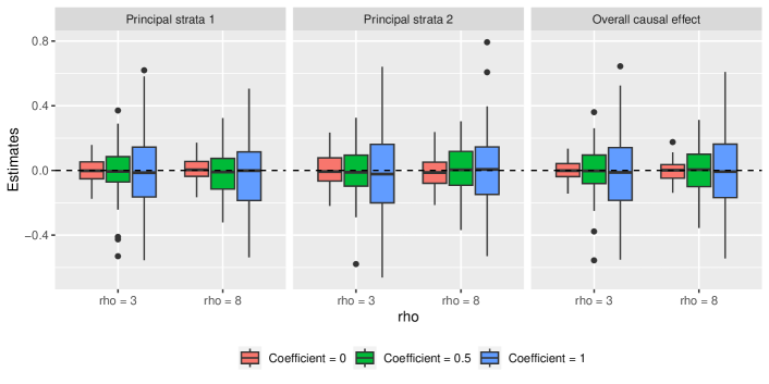
Figure 9: Distribution of point estimates minus the corresponding true values for two different principal causal effects, and the average causal effect. The sample size here is now $n=1000$.

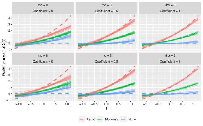
Figure 10: Estimates of $S(t)$ as a function of $t$ for each cluster of units. The dotted line corresponds to the true $\phi(t)$ for each cluster. The sample size here is now $n=1000$.

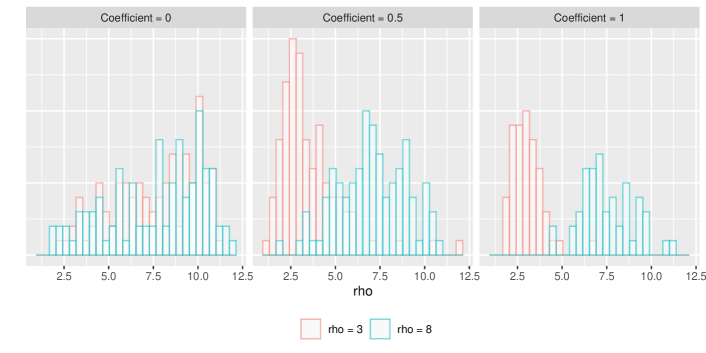
Figure 11: Distribution of point estimates for $\rho$ across all scenarios. The sample size here is now $n=1000$.

References

- Angrist et al., (1996) Angrist, J. D., Imbens, G. W., and Rubin, D. B. (1996). Identification of causal effects using instrumental variables. Journal of the American statistical Association, 91(434):444–455.
- Baccini et al., (2017) Baccini, M., Mattei, A., and Mealli, F. (2017). Bayesian inference for causal mechanisms with application to a randomized study for postoperative pain control. Biostatistics, 18(4):605–617.
- Bartolucci and Grilli, (2011) Bartolucci, F. and Grilli, L. (2011). Modeling partial compliance through copulas in a principal stratification framework. Journal of the American Statistical Association, 106(494):469–479.
- Bia et al., (2022) Bia, M., Mattei, A., and Mercatanti, A. (2022). Assessing causal effects in a longitudinal observational study with “truncated” outcomes due to unemployment and nonignorable missing data. Journal of Business & Economic Statistics, 40(2):718–729.
- Carmichael and Kent, (2014) Carmichael, J. T. and Kent, S. L. (2014). The persistent significance of racial and economic inequality on the size of municipal police forces in the united states, 1980–2010. Social Problems, 61(2):259–282.
- Chen et al., (2019) Chen, Y.-H., Mukherjee, B., and Berrocal, V. J. (2019). Distributed lag interaction models with two pollutants.
- Cheng and Small, (2006) Cheng, J. and Small, D. S. (2006). Bounds on causal effects in three-arm trials with non-compliance. Journal of the Royal Statistical Society: Series B (Statistical Methodology), 68(5):815–836.
- Escobar and West, (1995) Escobar, M. D. and West, M. (1995). Bayesian density estimation and inference using mixtures. Journal of the american statistical association, 90(430):577–588.
- Feller et al., (2016) Feller, A., Grindal, T., Miratrix, L., and Page, L. C. (2016). Compared to what? Variation in the impacts of early childhood education by alternative care type. The Annals of Applied Statistics, 10(3):1245 – 1285.
- Ferguson, (1973) Ferguson, T. S. (1973). A bayesian analysis of some nonparametric problems. The annals of statistics, pages 209–230.
- Forastiere et al., (2016) Forastiere, L., Mealli, F., and VanderWeele, T. J. (2016). Identification and estimation of causal mechanisms in clustered encouragement designs: Disentangling bed nets using bayesian principal stratification. Journal of the American Statistical Association, 111(514):510–525.
- Frangakis et al., (2004) Frangakis, C. E., Brookmeyer, R. S., Varadhan, R., Safaeian, M., Vlahov, D., and Strathdee, S. A. (2004). Methodology for evaluating a partially controlled longitudinal treatment using principal stratification, with application to a needle exchange program. Journal of the American Statistical Association, 99(465):239–249.
- Frangakis and Rubin, (2002) Frangakis, C. E. and Rubin, D. B. (2002). Principal stratification in causal inference. Biometrics, 58(1):21–29.
- Franks et al., (2020) Franks, A., D’Amour, A., and Feller, A. (2020). Flexible sensitivity analysis for observational studies without observable implications. Journal of the American Statistical Association, 115(532):1730–1746.
- Frumento et al., (2012) Frumento, P., Mealli, F., Pacini, B., and Rubin, D. B. (2012). Evaluating the effect of training on wages in the presence of noncompliance, nonemployment, and missing outcome data. Journal of the American Statistical Association, 107(498):450–466.
- Hirano et al., (2000) Hirano, K., Imbens, G. W., Rubin, D. B., and Zhou, X.-H. (2000). Assessing the effect of an influenza vaccine in an encouragement design. Biostatistics, 1(1):69–88.
- Imai, (2008) Imai, K. (2008). Sharp bounds on the causal effects in randomized experiments with “truncation-by-death”. Statistics & probability letters, 78(2):144–149.
- Imbens and Rubin, (1997) Imbens, G. W. and Rubin, D. B. (1997). Bayesian inference for causal effects in randomized experiments with noncompliance. The annals of statistics, pages 305–327.
- Jiang and Ding, (2021) Jiang, Z. and Ding, P. (2021). Identification of causal effects within principal strata using auxiliary variables. Statistical Science, 36(4):493–508.
- Jin and Rubin, (2008) Jin, H. and Rubin, D. B. (2008). Principal stratification for causal inference with extended partial compliance. Journal of the American Statistical Association, 103(481):101–111.
- Jo et al., (2011) Jo, B., Stuart, E. A., MacKinnon, D. P., and Vinokur, A. D. (2011). The use of propensity scores in mediation analysis. Multivariate Behavioral Research, 46(3):425–452.
- Kim et al., (2019) Kim, C., Daniels, M. J., Hogan, J. W., Choirat, C., and Zigler, C. M. (2019). Bayesian methods for multiple mediators: Relating principal stratification and causal mediation in the analysis of power plant emission controls. The annals of applied statistics, 13(3):1927.
- Lee, (2009) Lee, D. S. (2009). Training, wages, and sample selection: Estimating sharp bounds on treatment effects. The Review of Economic Studies, 76(3):1071–1102.
- Linero and Antonelli, (2023) Linero, A. R. and Antonelli, J. L. (2023). The how and why of bayesian nonparametric causal inference. Wiley Interdisciplinary Reviews: Computational Statistics, 15(1):e1583.
- Ma et al., (2011) Ma, Y., Roy, J., and Marcus, B. (2011). Causal models for randomized trials with two active treatments and continuous compliance. Statistics in Medicine, 30(19):2349–2362.
- (26) Mattei, A., Ding, P., Ballerini, V., and Mealli, F. (2023a). Assessing causal effects in the presence of treatment switching through principal stratification. arXiv preprint arXiv:2002.11989v2.
- (27) Mattei, A., Forastiere, L., and Mealli, F. (2023b). Assessing principal causal effects using principal score methods. In Handbook of Matching and Weighting Adjustments for Causal Inference, chapter 17, pages 313–348. Chapman and Hall/CRC.
- Mattei and Mealli, (2007) Mattei, A. and Mealli, F. (2007). Application of the principal stratification approach to the faenza randomized experiment on breast self-examination. Biometrics, 63(2):437–446.
- Mattei and Mealli, (2011) Mattei, A. and Mealli, F. (2011). Augmented designs to assess principal strata direct effects. Journal of the Royal Statistical Society: Series B (Statistical Methodology), 73(5):729–752.
- Mealli and Mattei, (2012) Mealli, F. and Mattei, A. (2012). A refreshing account of principal stratification. The international journal of biostatistics, 8(1).
- Mealli and Pacini, (2013) Mealli, F. and Pacini, B. (2013). Using secondary outcomes to sharpen inference in randomized experiments with noncompliance. Journal of the American Statistical Association, 108(503):1120–1131.
- Mealli et al., (2016) Mealli, F., Pacini, B., and Stanghellini, E. (2016). Identification of principal causal effects using additional outcomes in concentration graphs. Journal of Educational and Behavioral Statistics, 41(5):463–480.
- Mealli and Rubin, (2003) Mealli, F. and Rubin, D. B. (2003). Assumptions allowing the estimation of direct causal effects. Journal of Econometrics, 112(1):79–87.
- Neelon and Dunson, (2004) Neelon, B. and Dunson, D. B. (2004). Bayesian isotonic regression and trend analysis. Biometrics, 60(2):398–406.
- Reiss et al., (2017) Reiss, P. T., Goldsmith, J., Shang, H. L., and Ogden, R. T. (2017). Methods for scalar-on-function regression. International Statistical Review, 85(2):228–249.
- Ricciardi et al., (2020) Ricciardi, F., Mattei, A., and Mealli, F. (2020). Bayesian inference for sequential treatments under latent sequential ignorability. Journal of the American Statistical Association, 115(531):1498–1517.
- Rubin, (1974) Rubin, D. B. (1974). Estimating causal effects of treatments in randomized and nonrandomized studies. Journal of educational Psychology, 66(5):688.
- Rubin, (1980) Rubin, D. B. (1980). Randomization analysis of experimental data: The fisher randomization test comment. Journal of the American statistical association, 75(371):591–593.
- Rubin, (1981) Rubin, D. B. (1981). The bayesian bootstrap. The annals of statistics, pages 130–134.
- Rubin, (2004) Rubin, D. B. (2004). Direct and indirect causal effects via potential outcomes. Scandinavian Journal of Statistics, 31(2):161–170.
- Rusche and Kirchheimer, (1939) Rusche, G. and Kirchheimer, O. (1939). Punishment and social structure. Columbia University Press.
- Schwartz et al., (2011) Schwartz, S. L., Li, F., and Mealli, F. (2011). A bayesian semiparametric approach to intermediate variables in causal inference. Journal of the American Statistical Association, 106(496):1331–1344.
- Sethuraman, (1994) Sethuraman, J. (1994). A constructive definition of dirichlet priors. Statistica sinica, pages 639–650.
- Sjölander et al., (2009) Sjölander, A., Humphreys, K., Vansteelandt, S., Bellocco, R., and Palmgren, J. (2009). Sensitivity analysis for principal stratum direct effects, with an application to a study of physical activity and coronary heart disease. Biometrics, 65(2):514–520.
- Sutton, (2004) Sutton, J. R. (2004). The political economy of imprisonment in affluent western democracies, 1960–1990. American Sociological Review, 69(2):170–189.
- Ten Have and Joffe, (2012) Ten Have, T. R. and Joffe, M. M. (2012). A review of causal estimation of effects in mediation analyses. Statistical Methods in Medical Research, 21(1):77–107.
- VanderWeele, (2008) VanderWeele, T. J. (2008). Simple relations between principal stratification and direct and indirect effects. Statistics & Probability Letters, 78(17):2957–2962.
- Warren et al., (2022) Warren, J. L., Chang, H. H., Warren, L. K., Strickland, M. J., Darrow, L. A., and Mulholland, J. A. (2022). Critical window variable selection for mixtures: estimating the impact of multiple air pollutants on stillbirth. The Annals of Applied Statistics, 16(3):1633–1652.
- Wilson et al., (2020) Wilson, A., Tryner, J., L’Orange, C., and Volckens, J. (2020). Bayesian nonparametric monotone regression. Environmetrics, 31(8):e2642.
- Yang and Small, (2016) Yang, F. and Small, D. S. (2016). Using post-outcome measurement information in censoring-by-death problems. Journal of the Royal Statistical Society Series B: Statistical Methodology, 78(1):299–318.
- Zhang and Rubin, (2003) Zhang, J. L. and Rubin, D. B. (2003). Estimation of causal effects via principal stratification when some outcomes are truncated by “death”. Journal of Educational and Behavioral Statistics, 28(4):353–368.
- Zigler and Belin, (2012) Zigler, C. M. and Belin, T. R. (2012). A bayesian approach to improved estimation of causal effect predictiveness for a principal surrogate endpoint. Biometrics, 68(3):922–932.
- Zigler et al., (2012) Zigler, C. M., Dominici, F., and Wang, Y. (2012). Estimating causal effects of air quality regulations using principal stratification for spatially correlated multivariate intermediate outcomes. Biostatistics, 13(2):289–302.