Analysis of GWTC-3 with fully precessing numerical relativity surrogate models

Abstract

The third Gravitational-Wave Transient Catalog (GWTC-3) contains 90 binary coalescence candidates detected by the LIGO-Virgo-KAGRA Collaboration (LVK). We provide a re-analysis of binary black hole (BBH) events using a recently developed numerical relativity (NR) waveform surrogate model, NRSur7dq4, that includes all $\ell\leq 4$ spin-weighted spherical harmonic modes as well as the complete physical effects of precession. Properties of the remnant black holes’ (BH’s) mass, spin vector, and kick vector are found using an associated remnant surrogate model NRSur7dq4Remnant. Both NRSur7dq4 and NRSur7dq4Remnant models have errors comparable to numerical relativity simulations and allow for high-accuracy parameter estimates. We restrict our analysis to 47 BBH events that fall within the regime of validity of NRSur7dq4 (mass ratios greater than 1/6 and total masses greater than $60M_{\odot}$). While for most of these events our results match the LVK analyses that were obtained using the semi-analytical models such as IMRPhenomXPHM and SEOBNRv4PHM, we find that for more than 20% of events the NRSur7dq4 model recovers noticeably different measurements of black hole properties like the masses and spins, as well as extrinsic properties like the binary inclination and distance. For instance, GW150914_095045 exhibits noticeable differences in spin precession and spin magnitude measurements. Other notable findings include one event (GW191109_010717) that constrains the effective spin $\chi_{\mathrm{eff}}$ to be negative at a 99.3% credible level and two events (GW191109_010717 and GW200129_065458) with well-constrained kick velocities. Furthermore, compared to the models used in the LVK analyses, NRSur7dq4 recovers a larger signal-to-noise ratio and/or Bayes factors for several events. While these findings have important astrophysical implications, some of the more interesting events are affected by transient detector noise, which can be challenging to remove from short-duration signals.

I Introduction

The discovery of GW150914_095045 by the Advanced LIGO Harry (2010) and Virgo Acernese et al. (2015) detectors marked the beginning of gravitational-wave (GW) astronomy. Since then, during the first three observing runs (referred to as O1, O2, and O3) Abbott et al. (2019a, 2021a, 2021b, 2021c), the LVK Collaboration, consisting of LIGO and Virgo, together with the KAGRA Akutsu et al. (2021), has detected a total of $90$ gravitational wave events Abbott et al. (2021c). Several independent analyses of the public data have further revealed another $\sim 15$ events Venumadhav et al. (2020); Nitz et al. (2019, 2020, 2021). Analyses of the detected signals allow us to infer individual and population properties of merging compact objects  Abbott et al. (2019a, 2021a, 2021b); Venumadhav et al. (2020); Nitz et al. (2019, 2020, 2021); Fishbach et al. (2017); Wysocki et al. (2019); Abbott et al. (2019b); Roulet et al. (2020); Abbott et al. (2021d); Roulet et al. (2020); van Son et al. (2022); Payne and Thrane (2023); Doctor et al. (2020); Fishbach et al. (2021) including the existence of mass gaps and possible formation channels of binary black hole (BBH) systems Stevenson et al. (2015); Abbott et al. (2016a); Zevin et al. (2017); Abbott et al. (2017a). GW signals also encode information of the equation of state of the neutron-star matter Abbott et al. (2018); Most et al. (2018); Essick et al. (2020); Abbott et al. (2020a), the nature of gravity Yunes and Siemens (2013); Carson and Yagi (2019); Abbott et al. (2016b, 2021e, 2019c), environments around compact objects Barausse et al. (2015), and inform our understanding of cosmology by providing an independent measurement of the Hubble constant Abbott et al. (2017b, 2021f); Cantiello et al. (2018).

Inference of binary source properties from a detected signal relies on the availability of expedient and accurate gravitational waveform models that are capable of describing the entire coalescence from the inspiral through the binary merger and ringdown of the remnant object. Current GW models can be categorized into three sets: phenomenological models Husa et al. (2016); Khan et al. (2016); London et al. (2018); Khan et al. (2019); Hannam et al. (2014a); Khan et al. (2020); Pratten et al. (2021); Estellés et al. (2021, 2022a, 2022b, 2022b); Hamilton et al. (2021), effective-one-body (EOB) models Bohé et al. (2017); Cotesta et al. (2018a, 2020); Pan et al. (2014a); Babak et al. (2017a); Cotesta et al. (2020); Pan et al. (2014a); Babak et al. (2017a); Ossokine et al. (2020); Damour and Nagar (2014); Nagar et al. (2020a, b); Riemenschneider et al. (2021); Khalil et al. (2023); Pompili et al. (2023); Ramos-Buades et al. (2023); van de Meent et al. (2023), and numerical relativity (NR) surrogate models Blackman et al. (2015, 2017a, 2017b); Varma et al. (2019a, b); Islam et al. (2021a). The phenomenological and EOB waveform families are semi-analytical models that rely on a physically motivated ansatz, with calibration parameters that are fit to a set of NR simulations. NR surrogate models instead take a purely data-driven approach by training the model directly on NR simulations without the need for an ansatz. NR surrogates have been shown to be more accurate than semi-analytical models within their common regime of validity and capture the underlying physics in the NR simulations (such as precession) at an accuracy comparable to the simulations themselves Varma et al. (2019a, b); Blackman et al. (2017b). Consequently, NR surrogate models can provide highly accurate and trustworthy information about BBH source properties, especially as detector sensitivity improves Kumar et al. (2019); Islam et al. (2021b); Varma et al. (2022a); Abbott et al. (2020b).

Compared to phenomenological and EOB waveform models, however, surrogate models have a restricted regime of validity as they rely on the availability of NR simulations for training. The surrogate model we consider in this work, NRSur7dq4 Varma et al. (2019a), can only be evaluated for mass ratios $q\geq 1/6$, where $q:=m_{2,{\rm det}}/m_{1,{\rm det}}$; $m_{1,{\rm det}}$ and $m_{2,{\rm det}}$ are the masses of the primary and secondary black hole, respectively, in the detector frame. Furthermore, because of the computational limitations of NR simulations, NRSur7dq4 only supports relatively short duration signals ($\sim 20$ orbits), which further restricts its applicability to heavy binaries with a detector-frame total mass of $M_{\rm det}:=m_{1,{\rm det}}+m_{2,{\rm det}}\geq 60M_{\odot}$ These restrictions leave 47 events from GWTC-3 that can be analyzed with the NRSur7dq4 waveform model (see Section III for details).

In this paper, we present a thorough analysis of these 47 events using the NRSur7dq4 waveform model for binary source parameter inference and an associated NRSur7dq4Remnant model to infer the mass, spin vector, and kick vector of the final black hole remnant. Our work builds upon previous studies that applied NR surrogate models to special events such as the first observation Kumar et al. (2019), the first observation of a high-mass ratio BBH merger Islam et al. (2021b), a highly precessing system Varma et al. (2022b), and an intermediate-mass black hole formed through a BBH merger Abbott et al. (2020b). We also compare (i) NRSur7dq4 posteriors against publicly available LVK posteriors Abbott et al. (2021b, c); Collaboration and Collaboration (2022a); Collaboration et al. (2021a) obtained using the IMRPhenomXPHM Pratten et al. (2021) and SEOBNRv4PHM Ossokine et al. (2020) models, (ii) the recovered Bayes factors and differences in the signal-to-noise ratios (SNRs) between NRSur7dq4 and IMRPhenomXPHM, and (iii) the remnant mass and spin magnitude estimates obtained for the three models. We find that while, for most events, our results are consistent with the LVK analyses, more than 20% of events exhibit noticeably different measurements and some differences, such as constraining GW191109_010717’s effective spin to be confidently negative, may have important astrophysical implications.

The rest of the paper is organized as follows. Section II presents our analysis framework, including strain data, the NRSur7dq4 model, and our choice of priors, reference frame, and sampler settings. In Sec. III, we discuss how the set of 47 events that are analyzed have been selected. We provide an overview of the NRSur7dq4 results in Sec. IV and quantify the difference between NRSur7dq4 and IMRPhenomXPHM/SEOBNRv4PHM posteriors. The events that show the largest discrepancy with the LVK results are considered in more detail in Sec. IV.1 and Sec. IV.2. In Sec. V, we use Bayes factors and recovered SNRs to better understand whether the data has a preference for a particular model, finding the data shows mild support for the NRSur7dq4 model. Constraints on the mass, spin vector, and kick vector are considered in Sec. VI. Finally, in Sec. VII we summarize our results and discuss the implications of our findings. Our posterior samples are publicly available at Ref. T. et al. (2023).

II Data analysis framework

In this section, we summarize the Bayesian inference methods used in this study (Sec. II.1) and provide an overview of our data analysis framework. Our setup is mostly consistent with settings used to obtain the public LVK posteriors Abbott et al. (2021b, c); Collaboration and Collaboration (2022a); Collaboration et al. (2021a), with the relevant differences detailed in Sec. II.5 and II.6

II.1 Bayesian inference

The GW signal from a coalescing quasi-circular compact BBH system in general relativity can be completely characterized by a set of 15 parameters that we denote $\Theta=\{\mathcal{I},\mathcal{E}\}$. The parameter vector $\Theta$ consists of eight intrinsic parameters $\mathcal{I}$ and seven extrinsic parameters $\mathcal{E}$. The vector $\mathcal{I}:=\{m_{1},m_{2},\chi_{1},\chi_{2},\theta_{1},\theta_{2},\phi_{12},\phi_{\rm JL}\}$ contains the intrinsic parameters that describe the binary: the component masses $m_{1}$ and $m_{2}$ (with $m_{1}\geq m_{2}$), dimensionless spin magnitudes $\chi_{1}$ and $\chi_{2}$, spin tilt angles $\theta_{1}$ and $\theta_{2}$, and two azimuthl spin angles $\phi_{12}$ and $\phi_{\rm JL}$. The definition of these parameters is nicely summarized in Appendix E of Ref. Romero-Shaw et al. (2020). We further use $\bm{\chi_{1}}$ and $\bm{\chi_{2}}$ to denote spin vectors for each component black hole, $\bm{L}$ to denote the orbital angular momentum, and $\bm{J}$ to denote the total angular momentum. Moreover, we distinguish between the source-frame and detector-frame masses by using the subscript ‘det’. For example, $m_{1}$ is the source-frame mass and $m_{1,\rm det}$ the detector-frame mass of the primary black hole. These masses are related by $m_{1}=m_{1,{\rm det}}/(1+z)$ where $z$ is the redshift of the source. The set of extrinsic parameters $\mathcal{E}=\{\theta_{\rm JN},D_{\rm L},\alpha,\delta,\psi,\phi_{c},t_{c}\}$ parameterizes the location and orientation of the binary relative to the detectors as well as the coalescence time. The angle between the total angular momentum of the binary and the line-of-sight to the detector is denoted by $\theta_{\rm JN}$ (filling the role of the ‘inclination angle’) while the luminosity distance to the source is denoted by $D_{\rm L}$. Right ascension $\alpha$ and declination $\delta$ parameterize the location of the source in the sky, and $\psi$ is the polarization angle. The coalescence time is denoted by $t_{c}$ while $\phi_{c}$ indicates a reference orbital phase.

We use Bayes’ theorem to compute the posterior probability distribution of the binary parameters,

$$p(\Theta|\{d_{k}\},{\cal H})=\frac{{\cal L}(\{d_{k}\}|\Theta,{\cal H})\pi(\Theta|{\cal H})}{\mathcal{Z}(\{d_{k}\}|{\cal H})}\,,$$ (1)

where $\cal H$ is the signal hypothesis, $d_{k}(t)$ represents time-domain strain data for the $k^{th}$ detector,

$$d_{k}(t)=h_{k}(t;\Theta)+n_{k}(t)\,,$$ (2)

which is assumed to be a sum of the true signal $h_{k}(t;\Theta)$ and noise $n_{k}(t)$ in each detector. The subscript “k” on our signal model denotes that the observed signal will look different in different interferometers. The posterior $p(\Theta|\{d_{k}\},{\cal H})$ is the target for the parameter estimation analysis while the model evidence,

$$\mathcal{Z}(\{d_{k}\}|{\cal H})=\int d\Theta\pi(\Theta|{\cal H})\mathcal{L}(\{d_{k}\}|\Theta,{\cal H})\,,$$ (3)

is the target for hypothesis testing (sometimes referred to as model selection). The prior probability, $\pi(\Theta|\cal H)$, is a prescribed probability distribution and represents our initial assumptions about the parameters describing an individual binary. The likelihood function,

$$\mathcal{L}(\{d_{k}\}|\Theta,{\cal H})\propto\prod_{k}\mathrm{exp}\left(-\frac{1}{2}\langle d_{k}-h_{k}^{\cal H}(\Theta)|d_{k}-h_{k}^{\cal H}(\Theta)\rangle\right)\,,$$ (4)

describes how well each set of $\Theta$ matches the data. Here, $h_{k}^{\cal H}(\Theta)$ is the signal waveform generated from a specific waveform model as part of our hypothesis (we typically omit the superscript for brevity), and $\langle a|b\rangle$ is the noise-weighted overlap integral defined as

$$\langle a|b\rangle:=4\Re\int_{f_{\rm low}}^{f_{\rm high}}\dfrac{\tilde{a}(f)\tilde{b}^{*}(f)}{S_{n}(f)}df,$$ (5)

with $S_{n}(f)$ being the one-sided power spectral density (PSD) of the detector noise, a “$\sim$” indicates a Fourier transform operation, and $*$ represents the complex conjugate. The integration limits, $f_{\rm low}$ and $f_{\rm high}$, are chosen to reflect the sensitivity bandwidth of the detectors; specific values are given in Sec. II.6.

To quantify how much more likely that the data is described by a signal and not a noise process, we compute the Bayes factor,

$$\mathcal{B}=\frac{\mathcal{Z_{\cal H}}}{\mathcal{Z}_{n}},$$ (6)

where $\mathcal{Z_{\cal H}}=\mathcal{Z}(\{d_{k}\}|{\cal H})$ and $\mathcal{Z}_{n}$ denote, respectively, the evidence for a signal model $\cal H$ and a noise-only model.

II.2 Numerical relativity surrogate model

Surrogate models use NR waveforms as training data and build a highly accurate interpolant over the parameter space using a combination of reduced-order modeling Field et al. (2014, 2011), parametric fits, and non-linear transformations of the waveform data Blackman et al. (2017a). The NRSur7dq4 model Varma et al. (2019a) used in this paper is trained on 1528 NR simulations Varma et al. (2019a) and spans the 7-dimensional parameter space of spin-precessing binaries. The model includes all $\ell\leq 4$ spin-weighted spherical harmonic modes, as well as the precession frame dynamics and spin evolution of the black holes. While the model has been trained for mass ratio $1/4\leq q\leq 1.0$ and spins $0.0\leq\chi_{1,2}\leq 0.8$, it can be extrapolated to $q\geq 1/6$ and $\chi_{1,2}\leq 1.0$ Varma et al. (2019a); Walker et al. (2023). In its regime of validity, NRSur7dq4 improves upon semi-analytical models by about an order of magnitude in accuracy, in terms of mismatches against NR waveforms Varma et al. (2019a); Walker et al. (2023).

We compare our results with public LVK posteriors Abbott et al. (2021b, c) obtained using the IMRPhenomXPHM Pratten et al. (2021); García-Quirós et al. (2020); Pratten et al. (2020) and SEOBNRv4PHM Ossokine et al. (2020); Cotesta et al. (2018b) waveform models. IMRPhenomXPHM is a phenomenological model that includes the effects of precession and the $\{(\ell,m)\}=\{(2,\pm 2),(2,\pm 1),(3,\pm 3),(3,\pm 2),(4,\pm 4)\}$ modes in the coprecessing frame. SEOBNRv4PHM is an EOB model that also includes the effects of precession and the $\{(\ell,m)\}=\{(2,\pm 2),(2,\pm 1),(3,\pm 3),(4,\pm 4),(5,\pm 5)\}$ modes in the coprecessing frame modes. Importantly, while both IMRPhenomXPHM and SEOBNRv4PHM are calibrated against nonprecessing NR simulations, they are not calibrated against precessing simulations. Instead, they apply a frame-twisting procedure to approximately transform an aligned-spin waveform in the coprecessing frame to a precessing waveform in the inertial frame.

To infer the mass, spin vectors, and the kick velocity vector of the remnant black hole, we use the remnant surrogate model, NRSur7dq4Remnant Varma et al. (2019c, a). The NRSur7dq4Remnant model is trained on the same set of 1528 NR simulations as NRSur7dq4, and is applicable in the same region of parameter space. NRSur7dq4Remnant improves upon previous remnant models by an order of magnitude in accuracy, in terms of errors in remnant properties with respect to NR simulations Varma et al. (2019a).

II.3 Frame choice

All time-dependent binary parameters, such as the BH spins and the system’s orientation, are defined in a frame such that at some reference time ($t_{\rm ref}$), the $z$-axis is along the instantaneous angular momentum vector $\bm{L}$, the $x$-axis is along the line of separation from the less massive BH to the more massive BH, and the $y$-axis completes the right-handed triad. The reference point is defined as the time ($t_{\rm ref}$) during the binary evolution where the GW frequency in the coprecessing frame (defined as twice the time derivative of Eq. 3 of Ref. Varma et al. (2019a)) passes $f_{\rm ref}=20$ Hz. Following Ref. Schmidt et al. (2017), we refer to this frame as the wave frame at $f_{\rm ref}=20$ Hz. We measure all binary parameters at this reference frequency.

II.4 GW strain data

The strain $d(t)$, PSD, and detector calibration uncertainty data are obtained from the LVK public data releases Abbott et al. (2021g); Collaboration and Collaboration (2022a); Collaboration et al. (2021a); Collaboration and Collaboration (2022b); Collaboration et al. (2021b). We use the de-glitched strain data for certain events as summarized in Table 1. The publicly available PSDs were generated using the on-source BayesWave method Littenberg and Cornish (2015); Cornish and Littenberg (2015); Chatziioannou et al. (2019) while the effect of frequency-dependent uncertainties in amplitude and phase of the interferometer calibration on the parameter estimation of each event follows the methods of Refs. Farr W. M. (2014); Romero-Shaw et al. (2020). The signal’s geocentric trigger time, duration, and sampling rate are also taken from publicly available  data releases. In particular, the event trigger times that can be separately obtained from the Gravitational Wave Open Science Center (GWOSC) were not used as they can be inconsistent  with the times used for the LVK parameter estimation analyses. The GWTC-3 data release Abbott et al. (2021b, c); Collaboration and Collaboration (2022a); Collaboration et al. (2021a); Collaboration and Collaboration (2022b); Collaboration et al. (2021b) further describe the methods used for data conditioning and (where needed) deglitching.

Events with SEOBNRv4PHM	Events with de-glitched
posteriors missing in	strain data
public LVK datasets
GW190413_052954	GW190413_134308
GW190413_134308	GW190503_185404
GW190421_213856	GW190513_205428
GW190426_190642	GW190514_065416
GW190521_030229	GW190701_203306
GW190602_175927	GW191109_010717
GW190803_022701	GW200129_065458
GW190828_063405
GW190926_050336
GW190929_012149

Table 1: List of events for which SEOBNRv4PHM posteriors are absent in the publicly released LVK posteriors Abbott et al. (2021b, c); Collaboration and Collaboration (2022a); Collaboration et al. (2021a) as well as the events for which we use publicly available de-glitched strain data Collaboration and Collaboration (2022b); Collaboration et al. (2021b); deg .

II.5 Choice of prior

Our assumptions for the priors $\pi(\Theta|{\cal H})$ are identical to the LVK analyses of the GWTC-3 catalog Abbott et al. (2019a, 2021a, 2021b, 2021c) with additional restrictions on the mass ratio and the total mass of the binary:

• We choose uniform priors in the detector-frame component masses subject to the following constraints on the BBH system: (i) the chirp mass satisfies $12M_{\odot}\leq\mathcal{M}_{c,{\rm det}}\leq 400M_{\odot}$, (ii) the mass ratio satisfies $0.167\leq q\leq 1$, and (iii) the total mass satisfies $M_{\rm det}\geq 60M_{\odot}$, where the chirp mass Finn and Chernoff (1993) is defined as $\mathcal{M}_{c,\rm det}=\frac{(m_{1,\rm det}m_{2,\rm det})^{3/5}}{(m_{1,\rm det}+m_{1,\rm det})^{1/5}}$. The second and third constraints are imposed to restrict the analysis to NRSur7dq4’s region of validity; see Sec. III.

• Uniform priors are used for the dimensionless spin magnitudes ($0.0\leq\chi_{1,2}\leq 0.99$) of the binary, with spin orientations taken as uniform on the unit sphere.

• The prior on the luminosity distance assumes uniform source distribution in comoving volume and time as implemented in the UniformSourceFrame prior class in Ref Romero-Shaw et al. (2020) within $100$ Mpc $\leq D_{\rm L}\leq 10,000$ Mpc. For some events, we use a higher upper bound to ensure that the posterior is contained within the prior’s range.

• For the orbital inclination angle $\theta_{\rm JN}$, we assume a uniform prior over $-1\leq\cos(\theta_{\rm JN})\leq 1$.

• Priors on the sky location parameters, right ascension $\alpha$ and declination $\delta$, are assumed to be uniform over the sky with periodic boundary conditions for $\alpha$.

• For the time of coalescence, we assume a uniform prior over $t_{\rm geo}-0.1\leq t_{c}\leq t_{\rm geo}+0.1$ where $t_{\rm geo}$ is the geocentric trigger time.

II.6 Parameter estimation settings

Sampler	Parameters
Dynesty Speagle (2020)	live-points $=2000$
	tolerance $=0.1$
	nact $=50$

Table 2: Dynesty static nested sampling configuration parameters. We use $2000$ live points and sample away from a current live point with random walks. We require that the number of random walk steps taken in each chain is at least 50 (=nact) times the autocorrelation length of the chain. Sampling continues until the estimated contribution of the remaining prior volume to the evidence is less than $0.1$ (=tolerance).

Performing a parameter estimation analysis requires specifying numerous configuration options whose specific settings can impact the final inferred source parameters. We have chosen our analysis settings to match the LVK analyses of GWTC-3 as closely as possible based on what is documented in Ref. Abbott et al. (2021g) and in the public LVK data release Collaboration and Collaboration (2022a); Collaboration et al. (2021a); Collaboration and Collaboration (2022b); Collaboration et al. (2021b). We briefly describe the most important parameter estimation settings while pointing out differences when they arise. Our complete configuration and environment files are made publicly available T. et al. (2023).

To estimate source properties, we employ the publicly-available Bayesian inference libraries parallel-bilby Smith et al. (2020) (version 1.0.1) and bilby Ashton et al. (2019); Romero-Shaw et al. (2020) (version 1.1.5) together with the dynesty Speagle (2020) (version 1.0.1) nested sampling algorithm Skilling (2006a). We report some of the most important sampler configuration settings in Table 2. We have varied these values for several events to check our posteriors are sufficiently converged. We have also varied the number of processes used in our parallel-bilby computation. As documented in App. A, we notice that an important quantity to consider is live-points-per-process. When this number becomes too small, the computed posteriors are demonstrably inaccurate. Through extensive experimentation, we find that using 128 processes (corresponding to $\approx 16$ live-points-per-process) provides robust posterior computations. Finally, following the official LVK analyses Collaboration and Collaboration (2022a); Collaboration et al. (2021a); Collaboration and Collaboration (2022b); Collaboration et al. (2021b), for each event, we perform a total of four independent Bayesian inference runs with different initial random seeds to account for statistical randomness. We then combine the posteriors from these four analyses weighted by their individual evidences to compute the final posteriors. As an additional consistency check, for some events we have also compared posteriors with different initial seeds, finding no significant differences between these runs.

When computing the overlap integral in Eq.(5), we follow Ref. Collaboration and Collaboration (2022a, b); Collaboration et al. (2021a, b) and set the maximum frequency to be $f_{\rm high}=0.875\times f_{\rm PSD}$, where $f_{\rm PSD}$ is the largest frequency in the publicly available PSD data Collaboration and Collaboration (2022a); Collaboration et al. (2021a). The factor of $0.875$ is used to minimize roll-off effects caused by the application of a tapering window to the time-domain data as implemented in bilby. We set the minimum frequency to be $f_{\rm low}=20$Hz for most of the events, with notable exceptions being GW190521_030229 ($f_{\rm low}=11$Hz for all detectors; following Ref. Abbott et al. (2020c)) and GW190727_060333 ($f_{\rm low}=50$Hz for the L1 detector; following Ref. Abbott et al. (2021c) to exclude data that could be corrupted by the presence of a nearby glitch).

We call the NRSur7dq4 model through its LALSimulation interface lal . For generating NRSur7dq4 waveforms, and as discussed in Sec. II.3, we always use a reference frequency of $f_{\rm ref}=20$Hz when setting model parameters. Furthermore, we generate the full length of the surrogate waveform (about 20 orbits) by passing $f_{\rm min}=0$ to the waveform generator function. The important distinction between $f_{\rm low}$ and $f_{\rm min}$ is that $f_{\rm low}$ sets the lower limit for the overlap integral (5), while $f_{\rm min}$ sets the starting frequency of the waveform. By setting $f_{\rm min}=0$ we obtain the longest possible signal from NRSur7dq4.

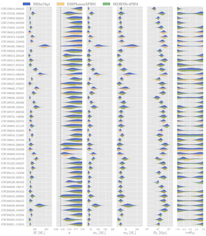
Figure 1: Posteriors for the source-frame total mass $M$, mass ratio $q$, source-frame component masses $m_{1}$, $m_{2}$, luminosity distance $D_{\rm L}$ and the cosine of the inclination angle $\theta_{\rm JN}$ for all 47 events analyzed with NRSur7dq4 model (blue). For comparison, we also show the public LVK posteriors Abbott et al. (2021b, c); Collaboration and Collaboration (2022a); Collaboration et al. (2021a) obtained using IMRPhenomXPHM (orange) and SEOBNRv4PHM (green) models. For some events, the SEOBNRv4PHM posteriors are missing from the LVK release (see Tab. 1); the SEOBNRv4PHM results are, therefore, also absent in this and all following figures for that subset of events. The grey dashed line represents the mass ratio cut of $q=1/6$ used for NRSur7dq4. Posteriors are reported in the wave frame (see Sec. II.3) at $f_{\rm ref}=20$ Hz. Further details are given in Sec. IV.

III Selection of events

One important limitation of NRSur7dq4 is the restricted duration of the waveforms provided by the model. The model is only able to generate relatively short duration waveforms corresponding to about $20$ orbits before merger, making it difficult to analyze low-mass systems ($M_{\rm det}\lesssim 60M_{\odot}$) when using a lower cut-off frequency of $f_{\rm low}=20$ Hz, the current default value for most LVK analyses Abbott et al. (2021b, c); Collaboration and Collaboration (2022a); Collaboration et al. (2021a). Furthermore, the model is valid only for binaries with a mass ratio in the range $1/6\leq q\leq 1$. This restricts the number of events we can analyze with the NRSur7dq4 model.

We inspect the public LVK posteriors of the binary source properties obtained using IMRPhenomXPHM Pratten et al. (2021) and SEOBNRv4PHM Ossokine et al. (2020) waveform models for all events in the GWTC-3 Abbott et al. (2021b, c); Collaboration and Collaboration (2022a); Collaboration et al. (2021a) catalog. We select the events for which at least 95% of the samples in the posteriors (inferred using the IMRPhenomXPHM model), have $M_{\rm det}$ larger than $60M_{\odot}$ and mass ratio $q$ larger than $0.167$. This ensures that these events fall within the domain of validity of the NRSur7dq4 model, which we also confirm after computing posteriors with the NRSur7dq4 model. A total of 47 BBH events that satisfy these criteria will be used in our analysis; these are listed in Figure 1.

IV Binary source parameter inference

We summarize our parameter inference results using NRSur7dq4 and NRSur7dq4Remnant for the 47 events selected from GWTC-3 Abbott et al. (2021b, c); Collaboration and Collaboration (2022a); Collaboration et al. (2021a) according to the procedure laid out in Sec. III. We then compare our results against the public LVK posteriors Abbott et al. (2021b, c); Collaboration and Collaboration (2022a); Collaboration et al. (2021a). While GWTC-2 Abbott et al. (2021a) also provides analyses of a subset of these events, including some results obtained using NRSur7dq4, to compare against the largest possible sample with the most consistent settings, we elide detailed comparisons to this earlier work for simplicity. For similar reasons, we also omit detailed comparison against other analyses of these events Venumadhav et al. (2020); Nitz et al. (2019, 2020, 2021).

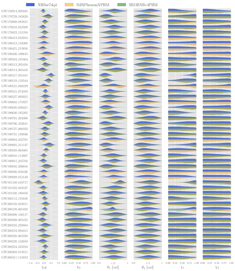
Figure 2: Posteriors for the spin magnitudes $\chi_{1}$ and $\chi_{2}$, spin angles $\theta_{1}$ and $\theta_{2}$, effective inspiral spin parameter $\chi_{\mathrm{eff}}$, and spin precession parameter $\chi_{p}$ for all 47 events analyzed with NRSur7dq4 model (blue). For comparison, we also show the public LVK posteriors Abbott et al. (2021b, c); Collaboration and Collaboration (2022a); Collaboration et al. (2021a) obtained using IMRPhenomXPHM in orange and SEOBNRv4PHM (where available) in green. Posteriors are reported in the wave frame (see Sec. II.3) at $f_{\rm ref}=20$ Hz. We provide 3D visualizations of the full spin posteriors at Ref. T. et al. (2023). Further details are given in Sec. IV.

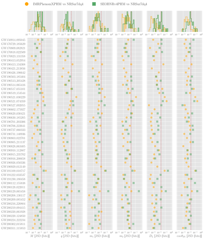
Figure 3: Jensen-Shannon divergence (JSD) values between the one-dimensional marginalized posteriors of the source-frame total mass $M$, mass ratio $q$, source-frame component masses $m_{1}$, $m_{2}$, luminosity distance $D_{\rm L}$ and the inclination angle $\theta_{\rm JN}$ obtained using NRSur7dq4 and the public LVK posteriors Abbott et al. (2021b, c); Collaboration and Collaboration (2022a); Collaboration et al. (2021a) obtained using IMRPhenomXPHM (blue circles) and SEOBNRv4PHM (green squares, where available). Dashed red lines correspond to a JS divergence of 0.02, indicating significant differences between these posteriors. Further details are discussed in Sec. IV.

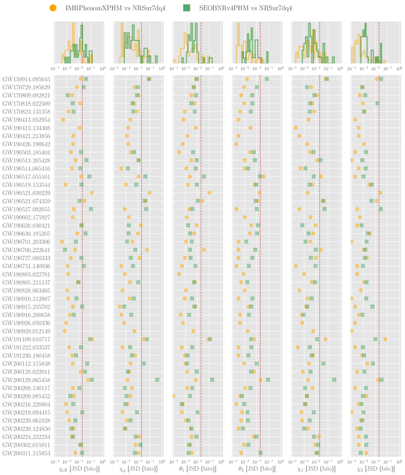
Figure 4: Jensen-Shannon divergence (JSD) values between the one-dimensional marginalized posteriors of the spin magnitudes $\chi_{1}$ and $\chi_{2}$, spin angles $\theta_{1}$ and $\theta_{2}$, effective inspiral spin parameter $\chi_{\mathrm{eff}}$ and spin precession parameter $\chi_{p}$ obtained using NRSur7dq4 and the public LVK posterior samples Abbott et al. (2021b, c); Collaboration and Collaboration (2022a); Collaboration et al. (2021a) obtained using IMRPhenomXPHM (blue circles) and SEOBNRv4PHM (green squares, where available). Dashed red lines correspond to a JS divergence of 0.02, indicating significant differences between these posteriors. Further details are discussed in Sec. IV.

For each event we infer all 15 BBH source parameters discussed in Sec II.1, we present results  for a smaller set of summary observables: the source-frame total mass, mass ratio, dimensionless spin magnitudes $\chi_{i}$, dimensionless spin tilts $\theta_{i}$ between the spin vectors and the orbital angular momentum, the effective inspiral spin parameter Ajith et al. (2011); Santamaria et al. (2010); Vitale et al. (2017),

$$\chi_{\mathrm{eff}}=\frac{m_{1}\chi_{1}\cos\theta_{1}+m_{2}\chi_{2}\cos\theta_{2}}{m_{1}+m_{2}}\,,$$ (7)

and the transverse spin precession parameter Hannam et al. (2014b); Schmidt et al. (2015),

$$\chi_{p}=\max\left\{\chi_{1}\sin\theta_{1},\frac{q(4q+3)}{4+3q}\chi_{2}\sin\theta_{2}\right\}\,.$$ (8)

In Fig. 1, we show the recovery of source-frame masses as well as the distance and inclination angles; in the accompanying Fig. 2, we show the corresponding results for the inferred spin parameters. For comparison, in both figures we also show the results from the public LVK posteriors Abbott et al. (2021b, c); Collaboration and Collaboration (2022a); Collaboration et al. (2021a) obtained using the IMRPhenomXPHM and SEOBNRv4PHM models. Note that IMRPhenomXPHM posteriors are obtained with bilby Ashton et al. (2019) while SEOBNRv4PHM posteriors are obtained with RIFT Lange et al. (2018). For the events listed in Table 1, SEOBNRv4PHM results are absent from the public LVK data release Abbott et al. (2021b, c); Collaboration and Collaboration (2022a); Collaboration et al. (2021a) and, therefore, are also absent in our comparisons.

In Figs. 1 and 2, we find many events for which noticeable differences exist between posteriors inferred with NRSur7dq4, IMRPhenomXPHM, and SEOBNRv4PHM. We use a standard diagnostic – the Jensen-Shannon (JS) divergence Lin (1991) – to quantify the difference between the one-dimensional marginalized posteriors inferred with NRSur7dq4 model (this work) and the posteriors obtained using IMRPhenomXPHM and SEOBNRv4PHM models (from the publicly available LVK posteriors Abbott et al. (2021b, c); Collaboration and Collaboration (2022a); Collaboration et al. (2021a)). Recall the JS divergence (JSD) between two probability density functions $p(x)$ and $q(x)$,

$${\rm JSD}(p,q)=\frac{{\rm KLD}(p||m)+{\rm KLD}(q||m)}{2},$$ (9)

is defined as a symmetrized extension of the Kullback-Leibler divergence Kullback and Leibler (1951), where $m(x)=1/2(p+q)$ is the point-wise mean of $p(x)$ and $q(x)$ and ${\rm KLD}$,

$${\rm KLD}(p||q)=\int p(x)\log_{2}\frac{p(x)}{q(x)}dx,$$ (10)

is Kullback-Leibler divergence. When using a base-2 logarithm JS divergence values are given in the units of bits. A JS divergence value of $0$ bits signifies that the posteriors are identical, while a JS divergence value of $1$ bit corresponds to posterior distributions that have no statistical overlap at all. Values smaller than $2\times 10^{-3}$ bits can occur due to stochastic sampling and indicate statistically indistinguishable posterior samples Romero-Shaw et al. (2020). The threshold for non-negligible bias varies by study, where JSD values of 0.007 Abbott et al. (2021a) (which for a Gaussian corresponds to a 20% shift in the mean), 0.02 Romero-Shaw et al. (2020), 0.05 Abbott et al. (2016c), and 0.15 Shaik et al. (2020) have all been used. In this paper, we will consider JSD values above 0.02 bits to indicate important differences between posteriors recovered from two different BBH waveform models Romero-Shaw et al. (2020).

In Fig. 3 and Fig. 4, for each event we show the JS divergence values between posterior distributions for the masses, spin, distance, and inclination angles (i.e., for the parameters shown in Fig. 1 and Fig. 2). We also show the distribution of the JS divergence values for all events for each of the parameters. At the top of each figure, We also show the distribution of the JS divergence values (over all events) for each of the parameters. We find that the JS divergence values between NRSur7dq4 and the IMRPhenomXPHM and SEOBNRv4PHM models are mostly less than 0.02 bits suggesting good agreement. However, for around $\sim 23$% ($\sim 55$%) of the analyzed events, JS divergence values between NRSur7dq4 and IMRPhenomXPHM (SEOBNRv4PHM) are larger than 0.02 bits for at least one of the parameters shown in Fig. 3 and Fig. 4. Such differences can arise from waveform systematics, such as the missing physics in IMRPhenomXPHM/SEOBNRv4PHM from not being informed by precessing NR simulations. We note, however, that at least some of the observed differences could arise from sampler techniques: bilby was used for IMRPhenomXPHM, RIFT for SEOBNRv4PHM, and parallel-bilby for NRSur7dq4. A more systematic study may be necessary to disentangle the specific origin of these differences.

IV.1 Highlighted events

Having provided an overview of the comparison of NRSur7dq4 posteriors against SEOBNRv4PHM and IMRPhenomXPHM results in Sec. IV, we now highlight certain events with noticeable differences in their inferred posteriors. For these events, Fig. 5 shows the posteriors for mass and spin parameters, while Fig. 6 focuses on the distance and inclination posteriors (with the total mass shown for comparison). Median values of the inferred source properties are given in Table  3 in the Appendix.

We reiterate that, for some of the events, SEOBNRv4PHM posteriors (obtained using the RIFT parameter estimation code) are missing in public LVK posteriors, as listed in Table 1. Furthermore, for several events where SEOBNRv4PHM posteriors are available due to an inefficient post-processing step incorporating the effects of calibration uncertainties in the GW data, the number of samples can be significantly reduced Payne et al. (2019, 2020). This results in the under-sampled posteriors for SEOBNRv4PHM visible for some events shown in Fig. 5 and Fig. 6.

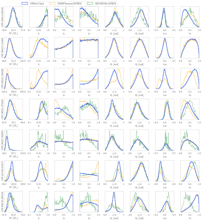
Figure 5: Posteriors for the source-frame total mass $M$, mass ratio $q$, spin magnitudes $\chi_{1}$ and $\chi_{2}$, spin angles $\theta_{1}$ and $\theta_{2}$, effective inspiral spin parameter $\chi_{\mathrm{eff}}$, and spin precession parameter $\chi_{p}$ for a list of seven events for which we infer the most significant differences between results obtained using NRSur7dq4 (blue histogram), IMRPhenomXPHM (orange histogram) and SEOBNRv4PHM (green histogram, where available). The under-sampled posteriors for SEOBNRv4PHM is a consequence of an inefficient post-processing procedure used in the RIFT code whenever calibration uncertainties are accounted for Payne et al. (2019, 2020). Posteriors are reported in the wave frame (see Sec. II.3) at $f_{\rm ref}=20$ Hz. Further details are given in Sec. IV.1.

IV.1.1 GW150914_095045: first GW observation

GW150914_095045 was the first direct GW observation and, with an SNR of $\sim 26$ Abbott et al. (2016c), remains one of the loudest events detected. This event has been extensively studied using a variety of waveform models over the past several years  Abbott et al. (2016c); Kumar et al. (2019); Mateu-Lucena et al. (2022); Abbott et al. (2017c). We find that while most of the marginalized posterior distributions match across waveform models, the distributions describing the spin parameters do not, as can be seen in the top row of Fig. 5.

In Fig. 5 (top row), we show that NRSur7dq4 favors smaller values for the spin magnitudes $\chi_{1}$ and $\chi_{2}$ compared to IMRPhenomXPHM and SEOBNRv4PHM. We also observe significant differences in the $\chi_{p}$ posteriors (Fig. 7a), where NRSur7dq4 favors smaller $\chi_{p}$ values than IMRPhenomXPHM and SEOBNRv4PHM. Fig. 7b summarizes the JS divergence values for many of the most interesting parameters. Interestingly, as highlighted in Fig. 7a, the NRSur7dq4 posterior for $\chi_{p}$ matches more closely with earlier estimates from GWTC-1 Abbott et al. (2016c) using the IMRPhenomPv2 Hannam et al. (2014b); Husa et al. (2016); Khan et al. (2016) (which does not include higher order modes) and SEOBNRv3 Pan et al. (2014b); Taracchini et al. (2014); Babak et al. (2017b) (which do not include $\ell>2$ modes) models. While we cannot offer a simple explanation for this tension between models, especially as the different models also rely on different posterior samplers, this might point to systematic differences arising from the treatment of precession or whenever subdominant harmonic modes play a role.

IV.1.2 GW190413_134308

For GW190413_13430 we find noticeable differences in the mass ratio (second row of Fig. 5), luminosity distance and inclination (first column of Fig. 6). The JS divergence values between the one-dimensional marginalized posteriors recovered with NRSur7dq4 and IMRPhenomXPHM are 0.031 bits (for $q$), 0.05 bits (for $D_{\rm L}$), and 0.026 bits (for $\theta_{\rm JN}$). We cannot compare with SEOBNRv4PHM because the corresponding posteriors are missing from the most recent LVK release.

IV.1.3 GW190521_030229

GW190521_030229 Abbott et al. (2020c, d) has unusually high component masses, $85^{+21}_{-14}$ $M_{\odot}$ and $66^{+17}_{-18}$ $M_{\odot}$, compared to other events. Consequently, the observable signal contains only a few pre-merger cycles. Furthermore, this event shows tentative signs of precession Abbott et al. (2020c, d); Biscoveanu et al. (2021); Estellés et al. (2022c); Nitz and Capano (2021). As a result, systematic differences between waveform models in the treatment of both precession and the merger-ringdown can play a more significant role for signals like this one. For example, Refs. Abbott et al. (2020b); Estellés et al. (2022c); Nitz and Capano (2021) already pointed out several systematic differences between NRSur7dq4 and other models for this event, and the same can be seen in Figs. 5 (third row) and 6 (second column). In particular, IMRPhenomXPHM prefers more unequal mass ratios with a clear bimodal mass ratio distribution while the NRSur7dq4 posterior shows visibly different features Estellés et al. (2022c); Nitz and Capano (2021) (third row of Fig. 5). Similarly, the posteriors for several spin parameters, including $\chi_{1}$, $\chi_{2}$, $\theta_{1}$, $\theta_{2}$, $\chi_{\mathrm{eff}}$ and $\chi_{p}$ in Fig. 5 indicate significant systematic differences between NRSur7dq4 and IMRPhenomXPHM. The JS divergence values between the one-dimensional marginalized posteriors recovered with NRSur7dq4 and IMRPhenomXPHM are 0.043 bits (for $M$), 0.136 bits (for $q$), 0.002 bits (for $\chi_{1}$), 0.025 bits (for $\chi_{2}$), 0.102 bits (for $\theta_{1}$), 0.017 bits (for $\theta_{2}$), 0.126 bits (for $\chi_{\mathrm{eff}}$) and 0.092 bits (for $\chi_{p}$). Among the extrinsic parameters, we find significant differences between the posteriors for $D_{\rm L}$ and $\theta_{\rm JN}$ (second column of Fig. 6), with JS divergence values of 0.083 bits and 0.107 bits, respectively. While we cannot compare with SEOBNRv4PHM as the corresponding posteriors are missing from the most recent LVK release  Abbott et al. (2021b, c); Collaboration and Collaboration (2022a); Collaboration et al. (2021a), such a comparison is shown in Ref. Abbott et al. (2020b), where significant differences were also noted between SEOBNRv4PHM and NRSur7dq4.

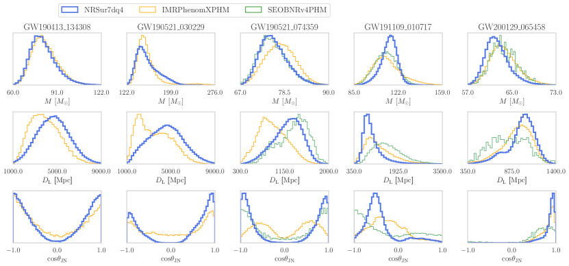
Figure 6: Posteriors for the source-frame total mass $M$, luminosity distance $D_{\rm L}$, and cosine of the inclination angle $\theta_{\rm JN}$ for a list of five events for which we see the largest differences between results obtained using NRSur7dq4 (blue histogram), IMRPhenomXPHM (orange histogram) and SEOBNRv4PHM (green histogram, where available). Further details are given in Sec. IV.1.

IV.1.4 GW190521_074359

Figures 5 (fourth row) and 6 (third column) show noticeable differences between NRSur7dq4 and the other models for several parameters for this event. In particular, NRSur7dq4 and SEOBNRv4PHM yield similar posteriors for the source-frame total mass $M$ whereas IMRPhenomXPHM favors slightly larger values for $M$. NRSur7dq4 also favors a slightly more asymmetric binary i.e., smaller values for $q$ compared to the other two models. Furthermore, we find noticeable differences in the $\chi_{1}$, $\chi_{2}$, and $\chi_{p}$ posteriors between three models, with the NRSur7dq4 falling broadly in between IMRPhenomXPHM and SEOBNRv4PHM. The JS divergence values between NRSur7dq4 and IMRPhenomXPHM (SEOBNRv4PHM) posteriors for $M$, $q$, $\chi_{1}$, $\chi_{2}$ and $\chi_{p}$ are 0.04 bits, 0.016 bits, 0.036 bits, 0.013 bits, and 0.047 bits (0.004 bits, 0.035 bits, 0.042 bits, 0.005 bits, and 0.036 bits), respectively. We further find noticeable differences between NRSur7dq4 and IMRPhenomXPHM (SEOBNRv4PHM [to a lesser extent]) posteriors for $D_{\rm L}$ and $\theta_{\rm JN}$ (third column of Fig. 6), with JS divergence values of 0.172 bits and 0.234 bits (0.04 bits and 0.07 bits), respectively.

IV.1.5 GW190527_092055

GW190527_092055 presents an interesting case as we find that, for almost all parameters shown in Fig.5 (fifth row), NRSur7dq4 and IMRPhenomXPHM yield consistent posteriors while SEOBNRv4PHM posteriors show noticeable differences. For example, both NRSur7dq4 and IMRPhenomXPHM posteriors for spin magnitudes $\chi_{1}$ and $\chi_{2}$ are uninformative whereas SEOBNRv4PHM posteriors show strong support for smaller values of $\chi_{1}$ and $\chi_{2}$ (fifth row of Fig. 5). The JS divergence values between NRSur7dq4 and IMRPhenomXPHM (SEOBNRv4PHM) posteriors for $\chi_{1}$ and $\chi_{2}$ are 0.0004 bits and 0.0003 bits (0.05 bits and 0.03 bits) respectively. Posteriors for the spin angles $\theta_{1}$ and $\theta_{2}$, however, match for all models (fifth row of Fig. 5). However, the SEOBNRv4PHM posteriors (obtained using the RIFT code) for this event appear to be particularly under-sampled, making it difficult to disentangle model systematics from sampler systematics. We note that Ref. Ángel Garrón and Keitel (2023) reanalyzed this event using parallel-bilby with NRSur7dq4 and obtained results consistent with ours. However, Ref. Dax et al. (2023) employed a machine-learning based parameter estimation code Dax et al. (2021) with importance sampling to reanalyze this event with SEOBNRv4PHM, finding better agreement between SEOBNRv4PHM and IMRPhenomXPHM.

IV.1.6 GW191109_010717

GW191109_010717 is another event that shows interesting and astrophysically important differences between posteriors obtained using the NRSur7dq4, IMRPhenomXPHM, and SEOBNRv4PHM models. For mass ratio $q$ and spin magnitude $\chi_{1}$, IMRPhenomXPHM posteriors show bimodalities whereas NRSur7dq4 and SEOBNRv4PHM posteriors do not (sixth row of Fig. 5). Another noteworthy observation is that IMRPhenomXPHM favors larger values for the secondary spin magnitude $\chi_{2}$ (sixth row of Fig. 5), whereas both NRSur7dq4 and SEOBNRv4PHM present posteriors for $\chi_{2}$ that are effectively uninformative. Furthermore, NRSur7dq4 shows a stronger preference for negative $\chi_{\mathrm{eff}}$ at 99.3% credible level, compared to 95.9% for SEOBNRv4PHM  and 85.3% for IMRPhenomXPHM. For IMRPhenomXPHM, we also see a bimodality in $\chi_{\mathrm{eff}}$, which likely results from the bimodality in $q$, due to the correlation between these two parameters. Furthermore, we note that the spin angle $\theta_{1}$ is well measured for this event but noticeably different across waveform models. Finally, the $\chi_{p}$ posteriors are also noticeably different across the models. The JS divergence values between NRSur7dq4 and IMRPhenomXPHM (SEOBNRv4PHM) posteriors for $q$, $\chi_{1}$, $\chi_{2}$, $\chi_{\mathrm{eff}}$, $\chi_{p}$ and $\theta_{1}$ are 0.091 bits, 0.062 bits, 0.067 bits, 0.139 bits, 0.029 bits and 0.082 bits (0.072 bits, 0.012 bits, 0.009 bits, 0.086 bits, 0.056 bits and 0.117 bits) respectively.

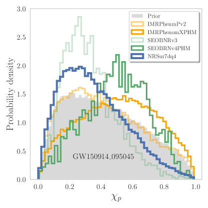
(a)

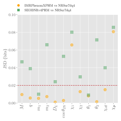
(b)

Figure 7: (a) Posteriors and priors for the spin precession parameter $\chi_{p}$ (computed in the wave frame at $f_{\rm ref}=20$ Hz) of GW150914_095045 obtained using NRSur7dq4 (blue histogram), IMRPhenomXPHM (orange histogram) and SEOBNRv4PHM (green histogram). For comparison, we also show posteriors obtained in earlier LVK studies (GWTC-1) using IMRPhenomPv2 (light orange) and SEOBNRv3 (light green). Somewhat surprisingly, the NRSur7dq4 posterior agrees more closely with older IMRPhenomPv2 and SEOBNRv3 models that do not include $\ell>2$ subdominant modes. (b) Jensen-Shannon divergence (JSD) values between the one-dimensional marginalized posteriors for a set of parameters (shown in Fig.3 and Fig.4) obtained using NRSur7dq4 and the public LVK posterior samples Abbott et al. (2021b, c); Collaboration and Collaboration (2022a); Collaboration et al. (2021a) obtained using IMRPhenomXPHM (blue circles) and SEOBNRv4PHM (green squares). Dashed red lines correspond to a JS divergence of 0.02, indicating significant differences between these posteriors. Further details are given in Sec. IV.1.1.

Among the extrinsic parameters, NRSur7dq4 provides more tightly constrained posteriors for the luminosity distance $D_{\rm L}$ and inclination $\theta_{\rm JN}$ (fourth column of Fig. 6). The JS divergence values between NRSur7dq4 and IMRPhenomXPHM (SEOBNRv4PHM) posteriors for $D_{\rm L}$ and $\theta_{\rm JN}$ are 0.081 bits and 0.107 bits (0.278 bits and 0.138 bits) respectively.

The strong preference for $\chi_{\mathrm{eff}}<0$ can have important astrophysical implications, as negative $\chi_{\mathrm{eff}}$ is expected to be more common in dynamically formed binaries than those formed through isolated evolution Mandel and O’Shaughnessy (2010); Rodriguez et al. (2016). We note, however, that de-glitched strain data is used for this event. Previous work on GW200129_065458 has shown potentially subtle issues can arise when using de-glitched strain data Payne et al. (2022). We refer to the dedicated glitch subtraction study presented for this and several other events in Ref. Davis et al. (2022) and Ref. Abbott et al. (2021h). Importantly, Ref. Abbott et al. (2021h) found (see their App. A) that transient non-gaussian noise or glitches affecting the data around the time of this event led to false violations of GR in the tests conducted in that work. Such effects could also impact the inference of $\chi_{\mathrm{eff}}$ (see e.g. App. B of Ref. Davis et al. (2022)).

IV.1.7 GW200129_065458

Next, we look at GW200129_065458 - another event where glitch subtraction was necessary Collaboration et al. (2021b); Payne et al. (2022), thereby complicating a straightforward interpretation of the signal. This event has many interesting properties: it has a network matched-filter SNR of 26.8 Abbott et al. (2021c) making it the loudest detected BBH signal, it has observable spin-induced orbital precession Hannam et al. (2022), and the post-merger remnant BH has a large recoil velocity Varma et al. (2022b).

Comparing the posteriors for NRSur7dq4, SEOBNRv4PHM, and IMRPhenomXPHM, we find noticeable differences for several parameters in Fig. 5 (seventh row) and Fig. 6 (fifth column). For example, NRSur7dq4 and IMRPhenomXPHM posteriors exhibit varying degrees of bimodality in mass ratio $q$ while SEOBNRv4PHM posteriors are uni-modal. Furthermore, NRSur7dq4 and IMRPhenomXPHM favor smaller (more unequal) values of $q$ than SEOBNRv4PHM. We also find significant differences in $\chi_{p}$ estimates between NRSur7dq4 and SEOBNRv4PHM (seventh row of Fig. 5) while IMRPhenomXPHM posteriors are consistent with NRSur7dq4. We note that our NRSur7dq4 posteriors for $\chi_{p}$ match the results obtained in Ref. Hannam et al. (2022). Similarly, for $\theta_{1}$ and $\theta_{2}$, NRSur7dq4 and SEOBNRv4PHM posteriors show noticeable differences whereas IMRPhenomXPHM broadly agrees with NRSur7dq4. The JS divergence values between NRSur7dq4 and IMRPhenomXPHM (SEOBNRv4PHM) posteriors for $q$, $\chi_{1}$, $\chi_{2}$, $\chi_{\mathrm{eff}}$, $\chi_{p}$, $\theta_{1}$ and $\theta_{2}$ are 0.023 bits, 0.002 bits, 0.017 bits, 0.063 bits, 0.001 bits, 0.008 bits and 0.008 bits (0.378 bits, 0.331 bits, 0.033 bits, 0.129 bits, 0.405 bits, 0.174 bits and 0.09 bits) respectively.

Finally, we also find significant differences between NRSur7dq4 and IMRPhenomXPHM (SEOBNRv4PHM) posteriors for $D_{\rm L}$ and $\theta_{\rm JN}$ (fifth column of Fig. 6), with JS divergence values of 0.025 bits and 0.029 bits (0.124 bits and 0.228 bits), respectively. We note that NRSur7dq4 favors larger values for $D_{\rm L}$ than both the IMRPhenomXPHM and SEOBNRv4PHM models.

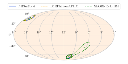
(a) GW190727_060333

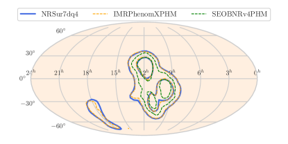
(b) GW200220_061928

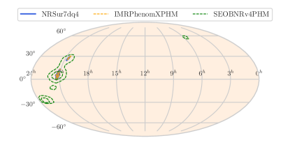
(c) GW200129_065458

Figure 8: Skymaps for three events where noticeable differences are observed between NRSur7dq4 (blue), IMRPhenomXPHM (orange), and SEOBNRv4PHM (green). We note that the discrepancies between SEOBNRv4PHM and the other models may arise from a different sampler used for the analysis with SEOBNRv4PHM. Further details are given in Sec IV.2.

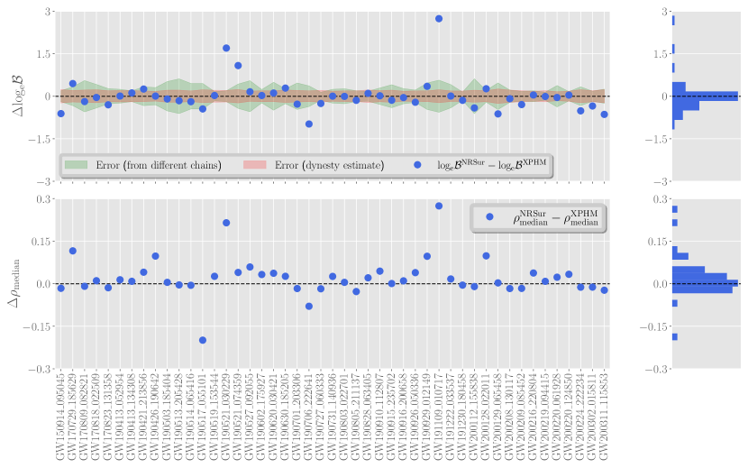
Figure 9: Differences in the recovered log Bayes factors $\Delta{\rm log_{e}}\mathcal{B}$ (upper panel) and the median SNR $\Delta\rho_{\rm median}$ (lower panel) between NRSur7dq4 (referred to as ‘NRSur’) and IMRPhenomXPHM models (referred to as ‘XPHM’) for all 47 events These events were analyzed using the prior described in Sec. II.5, which is restricted to a smaller portion of the parameter space as compared to the official LVK prior but matches the one used for our NRSur7dq4 analysis. We also show the estimated uncertainty in the calculation of the log evidence from parallel-bilby as a shaded red patch (upper panel). On the other hand, the shaded green patch (upper panel) shows the uncertainties estimated from four independent Bayesian inference runs with different random seeds. Further details are given in Sec. V.

IV.2 Sky localization

Next, we investigate whether NRSur7dq4 posteriors yield better constrained sky localization when compared to the public LVK posteriors obtained using the IMRPhenomXPHM and SEOBNRv4PHM models Abbott et al. (2021b, c); Collaboration and Collaboration (2022a); Collaboration et al. (2021a). For most events, NRSur7dq4, IMRPhenomXPHM, and SEOBNRv4PHM offer largely consistent skymaps.

In Fig. 8, we show the recovered skymaps for three events for which we notice the largest differences; the contours show regions containing the central 50% and 90% of the two-dimensional posterior distribution over sky angles - right ascension $\alpha$ and declination $\delta$. For each of the three events considered in Fig. 8, we find that the skymaps for NRSur7dq4 and IMRPhenomXPHM are consistent, while SEOBNRv4PHM shows a significant difference. It is important to recall that NRSur7dq4 and IMRPhenomXPHM posteriors are computed using parallel-bilby and bilby, respectively, and both employ the same dynesty sampler. The SEOBNRv4PHM posteriors are obtained with RIFT, which employs different sampling techniques over the extrinsic parameters. This is a potential reason for the differences in the skymap posteriors of SEOBNRv4PHM compared to the other models.

V Model selection

To understand whether the data prefers a particular waveform model, one can compare the Bayes factors, given in Eq. (6), for different models. For simplicity, we assume all models are equally likely, thereby sidestepping the issue of setting prior model odds. Even with this simplification, meaningfully comparing Bayes factors is complicated by the fact that the prior used for NRSur7dq4 in our study is restricted to a smaller portion of the parameter space  as compared to the ones used for IMRPhenomXPHM and SEOBNRv4PHM in the LVK analyses Abbott et al. (2021b, c); Collaboration and Collaboration (2022a); Collaboration et al. (2021a). Therefore, we re-analyze all 47 events considered in this paper using the IMRPhenomXPHM model with the same restricted priors and sampler settings (see Sec.II.6) used for the NRSur7dq4 runs. We do not perform any new parameter estimation runs with SEOBNRv4PHM due to the model’s high computational cost. Note that these IMRPhenomXPHM results obtained with redistricted priors are used only for meaningfully comparing the Bayes factors and SNRs in Fig. 9 and Fig. 16. For all other comparisons made throughout this paper, we use IMRPhenomXPHM results from the public LVK posteriors Abbott et al. (2021b, c); Collaboration and Collaboration (2022a); Collaboration et al. (2021a).

V.1 Bayes factors

We compute the differences,

$$\Delta\log_{e}\mathcal{B}=\log_{e}\mathcal{B}^{\rm NRSur}-\log_{e}\mathcal{B}^{\rm XPHM}\,,$$ (11)

where Eq. (11) is motivated by the identity

$$\frac{\mathcal{Z}(d|{\cal H}^{\rm NRSur})}{\mathcal{Z}(d|{\cal H}^{\rm XPHM})}=\frac{\mathcal{B}^{\rm NRSur}}{\mathcal{B}^{\rm XPHM}}\,.$$ (12)

Here $\mathcal{B}^{\rm NRSur}$ is the Bayes factor of NRSur7dq4 over noise hypothesis and $\mathcal{B}^{\rm XPHM}$ is the Bayes factor of IMRPhenomXPHM over noise hypothesis using the same priors used for the NRSur7dq4 analyses; see Eq. (6).

The log Bayes factor differences between NRSur7dq4 and IMRPhenomXPHM is shown in the upper panel of Fig. 9. We further provide associated error estimates for $\Delta\log_{e}\mathcal{B}$ (shaded red region), obtained using the error estimates for the logarithm of the waveform-model evidence provided by dynesty, and adding them in quadrature. We note, however, that this error band provides only a rough guide to indicate the accuracy achieved when computing the Bayes factor Skilling (2006b, 2004); Speagle (2020); Koposov et al. (2023). Indeed, we should view dynesty’s method for computing Bayes factors probabilistically, and the error estimation as a probabilistic statement (say, 1-sigma interval) instead of an error bound. For instance, in Fig. 9, we compare dynesty’s error estimate with the difference between the maximum and minimum log-Bayes factors (shaded green region) from the four independent Bayesian inference runs with different random seeds performed for each event (see Sec. II.6). This provides an an alternative estimate of the errors in the log-Bayes factors . We find that, for at least some events, the difference in log Bayes factor between the runs with different seeds can be larger than the error estimate in log Bayes factor provided by dynesty/parallel-bilby. This is not surprising in light of dynesty’s probabilistic error estimation Skilling (2006b, 2004); Speagle (2020); Koposov et al. (2023), but it does mean that for any particular event a log Bayes factor value can fluctuate outside of the red shaded region (dynesty error estimate) due to stochastic sampling. The histogram’s bin size has been set to roughly a 1-sigma interval.

Combining all 47 events in Fig. 9, the cumulative $\Delta\log_{e}\mathcal{B}$ value for NRSur7dq4 over IMRPhenomXPHM is 0.54, suggesting an overall mild preference for NRSur7dq4. We find three events, GW191109_010717, GW190521_030229 and GW190521_074359, where there is a clear preference for NRSur7dq4, with $\Delta\log_{e}\mathcal{B}$ values of 2.73, 1.69, and 1.08, respectively. All three of these events were highlighted in Sec. IV.1 as showing noticeable differences in posteriors. Excluding these three events, the histogram in the top-right panel of Fig. 9 indicates that (i) most events show no preference for either model, and (ii) many events show a very mild preference for IMRPhenomXPHM, although, as noted above, the true errors in our Bayes factor computation may be larger than those indicated in Fig. 9 thereby spoiling a clear interpretation of small values for any particular event. GW190706_222641 shows the largest preference for IMRPhenomXPHM, with a $\Delta\log_{e}\mathcal{B}$ value of $-0.98$.

In summary, while the data shows a very mild preference for NRSur7dq4 over IMRPhenomXPHM, there are clear outlier events and secular trends in the distribution of Bayes factors. Outlier events, trends, and the robustness of our results are considered in App. B.

V.2 Network SNR

Next, we compute posteriors for the network-matched filter SNR, $\rho$, recovered by the NRSur7dq4 model for each event. We then compare the median values of the posteriors for $\rho$ against the ones obtained using IMRPhenomXPHM. In the lower panel of Fig. 9, we report the difference,

$$\Delta\rho_{\rm median}=\rho^{\rm NRSur}_{\rm median}-\rho^{\rm XPHM}_{\rm median}\,,$$ (13)

between the median network matched filter SNR recovered by NRSur7dq4 and IMRPhenomXPHM. In this case, as indicated in the histogram in the bottom-right panel of Fig. 9, we find NRSur7dq4 typically recovers larger SNRs. GW191109_010717 and GW190521_030229 show the largest preference for NRSur7dq4, with differences in median SNR of 0.28 and 0.22, respectively. On the other hand, GW190517_055101 shows the largest preference for IMRPhenomXPHM, with a difference in median SNR of -0.20. Outlier events, trends, and the robustness of our results are considered in App. B.

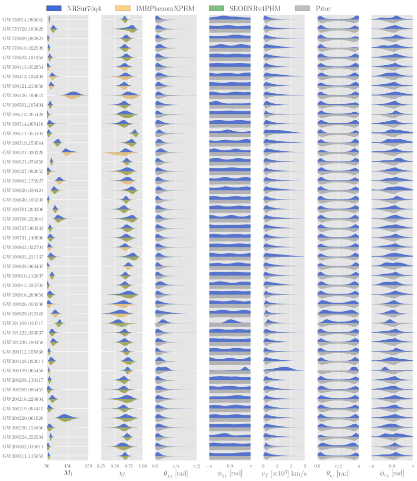
Figure 10: Posteriors for the source-frame remnant mass $M_{f}$, the remnant spin magnitude $\chi_{f}$, the remnant kick magnitude $v_{f}$, and the spherical polar $\{\theta_{\chi_{f}},\theta_{v_{f}}\}$ and azimuthal angles $\{\phi_{\chi_{f}},\phi_{v_{f}}\}$ of $\bm{\chi}_{f}$ and $\bm{v}_{f}$ for all 47 events analyzed with the NRSur7dq4 model (blue). For comparison, we also show the $M_{f}$ and $\chi_{f}$ posteriors from the public LVK data release Abbott et al. (2021b, c); Collaboration and Collaboration (2022a); Collaboration et al. (2021a) obtained using IMRPhenomXPHM (orange) and SEOBNRv4PHM (green, where available). For the rest of the parameters, we show the effective priors (in gray); the difference between the prior and posterior can be used to assess how informative the data are about these parameters. The spin and kick angles are shown in the wave frame at $t_{\rm ref}=-100\,M_{\rm det}$. We provide 3D visualizations of the full remnant spin and kick posteriors at Ref.  T. et al. (2023). Further details are given in Sec. VI.

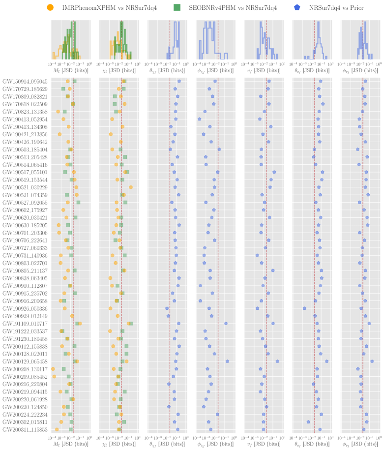
Figure 11: The first two columns show the JS divergence (JSD) for the source-frame remnant mass $M_{f}$ and spin magnitude $\chi_{f}$ between the NRSur7dq4 posteriors and the IMRPhenomXPHM (orange circles) and SEOBNRv4PHM (green squares, where available) posteriors from the LVK release Abbott et al. (2021b, c); Collaboration and Collaboration (2022a); Collaboration et al. (2021a). The remaining columns show the JS divergence for the remaining remnant parameters (same as Fig. 10) between the posterior and prior for NRSur7dq4 (blue pentagons). Dashed red lines indicate a JS divergence of 0.02, indicating significant differences between NRSur7dq4 and IMRPhenomXPHM/SEOBNRv4PHM posteriors for the first two columns, and informative NRSur7dq4 posteriors for the remaining columns. Further details are given in Sec. VI.

VI Inference of the remnant properties

In addition to constraining the properties of the component BHs in the binary, we infer the properties of the final BH left behind after the merger, in particular, its source-frame mass $M_{f}$, spin vector $\bm{\chi}_{f}$, and recoil velocity vector $\bm{v}_{f}$. During its evolution, the binary radiates energy, angular momentum, and linear momentum. The radiated energy and angular momentum are reflected in $M_{f}$ and $\bm{\chi}_{f}$, respectively. The radiated linear momentum causes a shift in the binary’s center of mass in the opposite direction, imparting a recoil velocity or a “kick” $\bm{v}_{f}$ to the remnant BH. While $\bm{\chi}_{f}$ is restricted to be either parallel or anti-parallel to the orbital angular momentum $\bm{L}$ for nonprecessing binaries, it can be arbitrarily oriented for precessing binaries. On the other hand, while the kicks for nonprecessing binaries are typically restricted to $\lesssim 300$ km/s and along the orbital plane, kicks for precessing binaries can reach magnitudes up to $\sim 5000$ km/s Campanelli et al. (2007); Gonzalez et al. (2007a); Lousto and Zlochower (2011); Gonzalez et al. (2007b) with arbitrary orientations. However, as we will discuss below, for precessing binaries, the direction of $\bm{\chi}_{f}$ is preferentially along, while the direction of $\bm{v}_{f}$ is preferentially along or opposite, the direction of $\bm{L}$ near merger.

Remnant BH properties have important applications for astrophysics and fundamental physics. The remnant mass and spin magnitude are important for tests of general relativity using GWs Abbott et al. (2021h), as the the remnant mass entirely determines frequencies in the ringdown and spin. The kick magnitude is important for placing observational constraints Varma et al. (2022b, 2020, c); Abbott et al. (2020b); Doctor et al. (2020); Mahapatra et al. (2021) on the rate of hierarchical mergers in dense environments: repeated mergers are a means to form heavy BHs in nature, but if the kick exceeds the escape velocity of the host environment, the remnant BH after the first merger would simply get ejected and not participate in another merger. Finally, the remnant spin direction and kick direction Varma et al. (2022b); Calderón Bustillo et al. (2022) can be useful to study binaries that may be formed in active galactic nuclei disks, as the final BH’s spin orientation with respect to the disk as well as its motion can impact potential electromagnetic counterparts Graham et al. (2020). The kick direction also shows up when computing the Doppler-shifted remnant mass, which may play a role in future high-accuracy ringdown tests of GR Varma et al. (2020, 2022b); Moore and Gerosa (2016); Mahapatra et al. (2023).

Therefore, while the public LVK results Abbott et al. (2021b, c); Collaboration and Collaboration (2022a); Collaboration et al. (2021a) only include the remnant mass and spin magnitudes, we provide posterior samples for the full spin and kick vectors. We report the source-frame mass $M_{f}$, spin vector $\bm{\chi}_{f}$ and kick velocity vector $\bm{v}_{f}$ of the remnant black hole for each of the 47 events we analyze in Fig. 10.

VI.1 Analysis framework

We follow the prescription outlined in Refs. Varma et al. (2020, 2022b, 2019a, 2019c): starting with the posterior samples for the spins and detector-frame component masses obtained using the NRSur7dq4 model, we evaluate the associated remnant surrogate model NRSur7dq4Remnant which provides estimates for $M_{f,{\rm det}}$, $\bm{\chi}_{f}$ and $\bm{v}_{f}$, from which we compute $M_{f}=M_{f,{\rm det}}/(1+z)$. These samples are included in our public release at Ref. T. et al. (2023). Note that the remnant spin and kick vectors in our public release are defined in the same frame as the component BHs, i.e. the wave frame at $f_{\rm ref}=20$ Hz, as described in Sec. II.3.

However, when visualizing the remnant spin and kick directions in this section, we adopt a different frame that is more naturally suited for discussing remnant properties: the wave frame at $t_{\rm ref}=-100\,M_{\rm det}$ as proposed in Ref. Varma et al. (2022a). This frame is similar to the wave frame at $f_{\rm ref}=20$ Hz (see Sec. II.3), except that the reference point is chosen to be the dimensionless time of $t_{\rm ref}=-100\,M_{\rm det}$ before the peak waveform amplitude (defined in Eq.5 of Ref. Varma et al. (2019a)). Because this reference point is always very close to the merger (typically within 2-4 GW cycles Varma et al. (2022a)), it provides a more natural frame to define remnant spin and kick vectors than the wave frame at $f_{\rm ref}=20$ Hz (which can occur up to $\sim 40$ GW cycles before the mergers for the events considered in this work).

For example, in the wave frame at $t_{\rm ref}=-100\,M_{\rm det}$, the direction of $\bm{\chi}_{f}$ is preferentially oriented close to the $z$-axis. This can be explained as follows: the direction of $\bm{\chi}_{f}$ can be approximated by the direction Barausse and Rezzolla (2009); Hofmann et al. (2016) of the total angular momentum $\bm{J}=\bm{L}+m_{1}^{2}\bm{\chi}_{1}+m_{2}^{2}\bm{\chi}_{2}$, but $\bm{J}$ is typically dominated (excluding the special case of transitional precession) by the contribution from $\bm{L}$ rather than the contribution from the spins. As a result, the direction of $\bm{\chi}_{f}$ is preferentially oriented close to $\bm{L}$ near merger, which is along the $z$-axis of the wave frame at $t_{\rm ref}=-100\,M_{\rm det}$ (see Sec. II.3). This is reflected in the prior for the remnant spin direction, as we will see in Sec. VI.4. Similarly, the wave frame at $t_{\rm ref}=-100\,M_{\rm det}$ is well-suited to discuss the kick direction as well, as the kick is known to be preferentially orientated close to or opposite to $\bm{L}$ near merger Campanelli et al. (2007); Gonzalez et al. (2007a); Lousto and Zlochower (2011); Gonzalez et al. (2007b); Varma et al. (2019c). For this reason, while our public release  T. et al. (2023) will contain remnant spin and kick vectors defined in the wave frame at $f_{\rm ref}=20$ Hz for consistency with the frame used for the component BH spins, in Figs. 10, 11, 12, 13, 14, we will adopt the wave frame at $t_{\rm ref}=-100\,M_{\rm det}$. As described in Ref. Varma et al. (2022a), the two frames are related by a transformation described by the dynamics of NRSur7dq4, which is provided by the model Varma et al. (2019a).

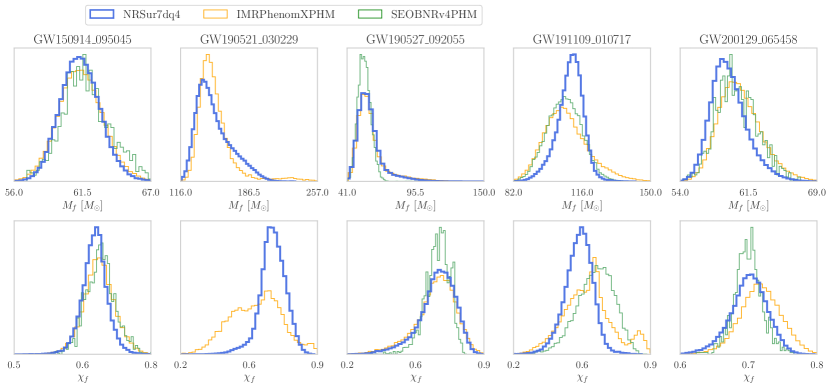
Figure 12: Posteriors of source-frame mass and spin magnitude of the remnant BH for five events where we see the most prominent differences between results obtained using NRSur7dq4 (blue histogram), IMRPhenomXPHM (orange histogram) and SEOBNRv4PHM (green histogram, where available). Further details are given in Sec. VI.2.

VI.2 Remnant mass and spin magnitude

Figure 10 summarizes our constraints on the remnant properties for all 47 events considered in our analysis (cf. Sec. III). The first two columns show the source-frame remnant mass $M_{f}$ and spin magnitude $\chi_{f}$ for NRSur7dq4 with NRSur7dq4Remnant, along with the corresponding constraints from the LVK public release for IMRPhenomXPHM and SEOBNRv4PHM  Abbott et al. (2021b, c); Collaboration and Collaboration (2022a); Collaboration et al. (2021a). In the LVK results, the remnant mass and spin magnitude are computed following Ref. Johnson-McDaniel et al. (2016), using the remnant models of Refs. Healy and Lousto (2017); Jiménez-Forteza et al. (2017); Hofmann et al. (2016). While these models include some precession corrections, they are not informed by precessing NR simulations. Therefore, differences with respect to our estimates of $M_{f}$ and $\chi_{f}$ can arise from differences in the remnant models as well as the waveform model used to infer binary source parameters.

The first two columns of Fig. 11 show the JS divergence between our posteriors for $M_{f}$ and $\chi_{f}$, and the public LVK samples for IMRPhenomXPHM and SEOBNRv4PHM. For about 13 % (17% ) of events, the JS divergence between NRSur7dq4 and IMRPhenomXPHM (SEOBNRv4PHM) for $M_{f}$ rises above 0.02 bits, indicating noticeable differences. Similarly, for about 19% (38%) of events, the JS divergence between NRSur7dq4 and IMRPhenomXPHM (SEOBNRv4PHM) for $\chi_{f}$ rises above 0.02 bits. The events with the most prominent differences are highlighted in Fig. 12.

Constraints on the remaining remnant parameters (the direction of $\bm{\chi}_{f}$, and the vector $\bm{v}_{f}$) are not provided in the public LVK samples Abbott et al. (2021b, c); Collaboration and Collaboration (2022a); Collaboration et al. (2021a). Therefore, in Figs. 10 and 11, we compare our posteriors for these parameters with their effective priors, to judge how informative the data are about these quantities. Following Refs. Varma et al. (2020, 2022b), effective prior samples for $M_{f}$ (not shown), $\bm{\chi}_{f}$ and $\bm{v}_{f}$ are obtained by evaluating the NRSur7dq4Remnant model on samples drawn from the prior on $\{m_{1},m_{2},\bm{\chi}_{1},\bm{\chi}_{2}\}$ (see Sec. II.5). In the following figures, the prior samples for $\bm{\chi}_{f}$ and $\bm{v}_{f}$ are also transformed to the wave frame at $t_{\rm ref}=-100\,M_{\rm det}$. To parameterize the remnant spin and kick directions, we adopt the standard spherical polar angles $\theta_{{\chi}_{f}}$ and $\theta_{v_{f}}$, and azimuthal angles $\phi_{{\chi}_{f}}$ and $\phi_{v_{f}}$, computed in the wave frame at $t_{\rm ref}=-100\,M_{\rm det}$.

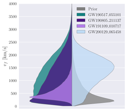
Figure 13: Kick magnitude constraints for four events with the largest JS divergence between the posterior and prior. We show the posteriors and the effective prior for comparison. GW200129_065458 and GW191109_010717 show a preference away from $v_{f}=0$. Further details are given in Sec. VI.3.

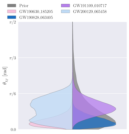
(a) $\theta_{\chi_{f}}$

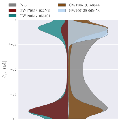
(b) $\theta_{v_{f}}$

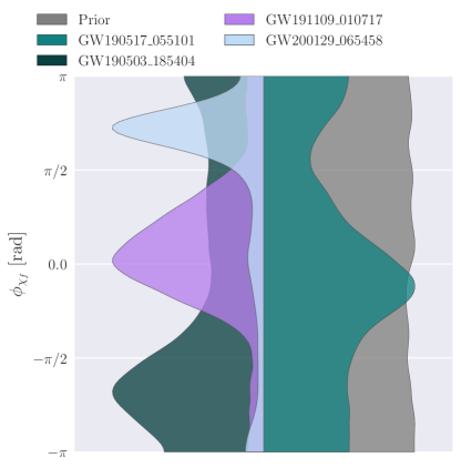
(c) $\phi_{\chi_{f}}$

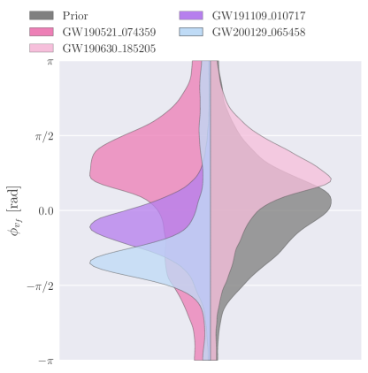
(d) $\phi_{v_{f}}$

Figure 14: Posteriors for the polar angles $\{\theta_{\chi_{f}},\theta_{v_{f}}\}$ and azimuthal angles $\{\phi_{\chi_{f}},\phi_{v_{f}}\}$ of the remnant black holes’ spin and kick directions for four events; these events are picked either because they show the highest JS divergence between posterior and prior, or because the posterior peaks noticeably away from the peak of the prior. We also show the effective priors in gray. The spin and kick angles are shown in the wave frame at $t_{\rm ref}=-100\,M_{\rm det}$. Further details are in the text (Sec. VI.4).

VI.3 Recoil velocity magnitude

The fifth column of Fig. 10 shows our constraints on the kick magnitude $v_{f}$ along with the corresponding prior. As expected from Ref. Varma et al. (2020), for most events the posterior is largely indistinguishable from the prior, meaning that the data are not informative about the kick magnitude. In Fig. 11, we find that the JS divergence between the posterior and prior of $v_{f}$ rises above 0.02 bits for about 36% of the events considered. The events with the four highest JS divergence values are highlighted in Fig. 13. Notably, two of these events show a clear preference away from $v_{f}=0$ compared to the prior: GW200129_065458 with $v_{f}\sim 1392^{+848}_{-1085}$ km/s and a JS divergence of 0.305 bits, and GW191109_010717 with $v_{f}\sim 485^{+668}_{-252}$ km/s and a JS divergence of 0.103 bits. Here, we report the median and 90% symmetric credible interval. While this finding can have important astrophysical implications, especially for hierarchical mergers, we again point out that both GW200129_065458 and GW191109_010717 suffered from being coincident with a detector glitch, which can be challenging to remove from short signals reliably such as these, potentially impacting inferences about precession and kicks Payne et al. (2022).

VI.4 Remnant spin and kick velocity directions

Finally, the remaining columns in Figs. 10 and 11 report the NRSur7dq4 posteriors and priors for the remnant spin and kick direction parameters. For each parameter ($\theta_{{\chi}_{f}}$, $\theta_{v_{f}}$, $\phi_{{\chi}_{f}}$ and $\phi_{v_{f}}$), we highlight four interesting events in Fig. 14. These events are picked either because they show the highest JS divergence between posterior and prior, or because the posterior peaks noticeably away from the peak of the prior.

Note that $\theta_{{\chi}_{f}}=0$ means that the spin is directed along $\bm{L}$ at $t_{\rm ref}=-100\,M_{\rm det}$. As mentioned above, binaries have a preference for $\theta_{{\chi}_{f}}=0$ in this frame, and this is reflected in the prior for $\theta_{{\chi}_{f}}$ having a strong preference for zero (Fig. 14a). Similarly, Fig. 14b shows that the prior for $\theta_{v_{f}}$ has a strong preference for zero or $\pi$, which was also motivated above. Finally, to orient the reader, we remind that $\phi_{{\chi}_{f}}=0$ ($\phi_{v_{f}}$=0) indicates that the in-plane component of the remnant spin (kick) is coaligned with a vector from the less massive BH to the more massive BH at $t_{\rm ref}=-100\,M_{\rm det}$. In Fig. 14, we note that while the prior for $\phi_{{\chi}_{f}}$ is broad, the prior for $\phi_{v_{f}}$ shows a preference for zero. These features highlight why the wave frame at $t_{\rm ref}=-100\,M_{\rm det}$ is a suitable frame for discussing remnant spin and kick directions.

In Fig. 11, we find that the JS divergence between the posterior and prior for $\theta_{{\chi}_{f}}$, rises above 0.02 bits for about 91.4% of the events considered, indicating that the data are informative about this parameter for most events. Among the highlighted events in Fig. 14a, GW190630_185205, GW190828_063405 and GW191109_010717 show a stronger preference for $\theta_{{\chi}_{f}}\sim 0$ than the prior, GW200129_065458 has a slightly bimodal posterior extending to $\theta_{{\chi}_{f}}\sim\pi/6$, and GW191109_010717 peaks at $\theta_{{\chi}_{f}}\sim\pi/12$, clearly away from the peak of the prior.

Next, for $\theta_{v_{f}}$, we find that JS divergence between the posterior and prior rises above 0.02 bits for about 89.3% of the events considered, indicating that this parameter may be more informative than the kick magnitude $v_{f}$ itself. Among the highlighted events in Fig. 14b, GW170818_022509 prefers a kick directed roughly along $\bm{L}$ at $t_{\rm ref}=-100\,M_{\rm det}$, while GW200129_065458 prefers the opposite. Here, we note that while GW200129_065458 shows a measurable kick magnitude, GW170818_022509 does not (see Fig. 10). Our findings are broadly consistent with the discussion of the measurability of the kick direction in Refs. Varma et al. (2020, 2022b); Calderón Bustillo et al. (2022), but more work may be needed to understand how to interpret $\theta_{v_{f}}$ constraints for events where the kick magnitude is unmeasured.

Finally, the JS divergence between the posterior and prior for $\phi_{{\chi}_{f}}$ and $\phi_{v_{f}}$ rises above 0.02 bits for about 6%, and 51% of the events considered, respectively. Therefore, the data are mostly uninformative about $\phi_{{\chi}_{f}}$, but can be used to constrain $\phi_{v_{f}}$. Among the highlighted events in Fig. 14c and 14d, GW191109_010717 and GW200129_065458 show the strongest constraints; clearly the kick direction is better measured than the kick magnitude.

VII Conclusion

The third Gravitational-Wave Transient Catalog contains 90 binary coalescence candidates detected by the LIGO-Virgo-KAGRA Collaboration. In this paper, we identify a set of 47 events from the GWTC-3 catalog Abbott et al. (2021b, c); Collaboration and Collaboration (2022a); Collaboration et al. (2021a) that falls within the domain of validity ($q\geq 1/6$ and $M_{\rm det}\geq 60M_{\odot}$) of the NRSur7dq4 waveform model (Sec. III). Within this domain, the NRSur7dq4 model about an order-of-magnitude more accurate than the models used in the the official LVK analysis and includes the full physical effects of precession. We use the Bayesian inference code parallel-bilby to estimate the source properties for these BBH events with the NRSur7dq4 model. We compare source properties inferred using the NRSur7dq4 model and public LVK posteriors obtained using the IMRPhenomXPHM and SEOBNRv4PHM models Abbott et al. (2021b, c); Collaboration and Collaboration (2022a); Collaboration et al. (2021a) (Sec. IV). The difference between the resulting posterior samples have been quantified using JS divergence, a common measure of the statistical distance in information content between probability distributions. We find many events for which noticeable differences exist between posteriors obtained with NRSur7dq4, IMRPhenomXPHM, and SEOBNRv4PHM models. Below are the key take-aways from our results:

• While the posteriors are consistent for the majority of events, we find a number of events for which posteriors for NRSur7dq4 are noticeably different from the posteriors for IMRPhenomXPHM/SEOBNRv4PHM. In particular, for $\sim 23$% ($\sim 55$%) of the analyzed events, JS divergence between NRSur7dq4 and IMRPhenomXPHM (SEOBNRv4PHM) exceeds a commonly used threshold of 0.02 bits, indicating non-negligible differences, for at least one of the following parameters: total mass $M$, mass ratio $q$, component masses $m_{1},m_{2}$, spin magnitudes $\chi_{1},\chi_{2}$, spin tilts $\theta_{1},\theta_{2}$, the effective inspiral spin $\chi_{\mathrm{eff}}$, the spin precession parameter $\chi_{p}$, luminosity distance $D_{\rm L}$, and inclination angle $\theta_{\rm JN}$ (Sec. IV). For many of these cases, multiple parameters exceed this threshold, and for a handful of events, the JS divergence values are above 0.1 (and in a few cases above 0.2) indicating substantial differences. The most interesting GW events are summarized in Sec. IV.1.

• Even for the first GW signal, GW150914_095045, we find noticeable differences in $\chi_{p}$ and $\chi_{1}$ measurements between NRSur7dq4, IMRPhenomXPHM and SEOBNRv4PHM. Interestingly, our NRSur7dq4 estimates show better agreement with earlier LVK results obtained with SEOBNRv3 and IMRPhenomPv2. Fig. 7 summarizes some of these observations.

• For GW191109_010717, NRSur7dq4 shows a stronger preference for negative $\chi_{\mathrm{eff}}$ at 99.3% credible level, compared to 95.9% for SEOBNRv4PHM and 85.3% for IMRPhenomXPHM (Sec. IV.1.6). This is consistent with Ref. Ramos-Buades et al. (2023), where a similar preference was found for the newer SEOBNRv5PHM model. The preference for $\chi_{\mathrm{eff}}<0$ can have important astrophysical implications, as negative $\chi_{\mathrm{eff}}$ is expected to be more common in dynamically formed binaries than those formed through isolated evolution. However, some caution is warranted as this event suffered from a detector glitch.

• The events showing the most notable differences in the posteriors for the component BH properties are highlighted in Sec. IV.1. Furthermore, by comparing the Bayes factors and recovered SNRs between NRSur7dq4 and IMRPhenomXPHM with the same prior settings for all 47 events, we find that there is a mild preference for NRSur7dq4 over IMRPhenomXPHM (Sec. V).

• We find several events where the remnant mass and spin magnitude posteriors are noticeably different between NRSur7dq4 and IMRPhenomXPHM/SEOBNRv4PHM, which can have implications for tests of general relativity (Sec. VI.2).

• We provide kick magnitude posteriors for all 47 events, which can be useful for constraining the formation rate of heavy BHs through repeated mergers (Sec. VI.3). We find that the kick magnitude is informative for GW191109_010717 and GW200129_065458, with GW200129_065458 showing a preference for a large kick, as noted by Ref. Varma et al. (2022b). However, once again, some caution is warranted as both of these events suffered from detector glitches.

• Finally, we also provide posteriors for the remnant spin and kick directions for all 47 events and discuss possible astrophysical applications of these measurements in Sec. VI.4.

The differences in the posteriors for NRSur7dq4, IMRPhenomXPHM and SEOBNRv4PHM suggest that waveform systematics are already important for GW data analysis. These differences can become compounded when the posterior samples are used in hierarchical analyses like constraining astrophysical populations or tests of general relativity. Systematic differences can arise from the differences in the modeling approach as well as the physics included; for example, while NRSur7dq4 is trained directly on precessing NR simulations, IMRPhenomXPHM and SEOBNRv4PHM are only informed by nonprecessing simulations.

However, we note that our comparisons are based on posteriors obtained using different Bayesian Inference codes: bilby for IMRPhenomXPHM, RIFT for SEOBNRv4PHM, and parallel-bilby for NRSur7dq4. This may introduce additional systematics in our attempts to make meaningful comparisons. For example, some of the SEOBNRv4PHM posteriors appear undersampled due to an inefficient post-processing step to include calibration uncertainties in RIFT (Fig. 5). Furthermore, we find that SEOBNRv4PHM posteriors for the skymaps are significantly different for a number of events while NRSur7dq4 and IMRPhenomXPHM match closely (Fig. 8). A more careful study will be necessary to fully disentangle waveform from sampler systematics.

Nonetheless, our results provide further motivation to improve all waveform models. In particular, it is important to extend the region of validity of NR surrogate models to include more unequal mass ratios as well as longer inspirals. As the detector sensitivities improve Pürrer and Haster (2020), systematic biases in estimating binary source parameters could limit important applications like BH astrophysics, dark siren cosmology Abbott et al. (2023), and fundamental tests of general relativity.

Our results are publicly accessible T. et al. (2023). We additionally provide an application programming interface (API) to access our data programmatically. The API is documented in the GitHub repository for this work T. et al. (2023). The catalog’s website utilized software from the TESS-Atlas project Foreman-Mackey and Vajpeyi .

Appendix A Posterior’s dependence on processes

	$M(M_{\odot})$	$q$	$m_{1}(M_{\odot})$	$m_{2}(M_{\odot})$	$\chi_{1}$	$\chi_{2}$	$\chi_{\rm eff}$	$\chi_{p}$	$D_{\rm L}$ (Gpc)	$\theta_{\rm JN}$ (rad)
GW150914_095045
NRSur7dq4	$64.3^{+3.0}_{-2.8}$	$0.86^{+0.12}_{-0.21}$	$34.61^{+4.47}_{-2.69}$	$29.73^{+2.74}_{-4.50}$	$0.26^{+0.47}_{-0.24}$	$0.32^{+0.52}_{-0.29}$	$-0.05^{+0.10}_{-0.12}$	$0.33^{+0.41}_{-0.25}$	$0.5^{+0.1}_{-0.1}$	$2.72^{+0.31}_{-0.46}$
IMRPhenomXPHM	$64.3^{+3.4}_{-3.2}$	$0.85^{+0.14}_{-0.22}$	$34.90^{+4.92}_{-2.98}$	$29.38^{+3.15}_{-4.99}$	$0.43^{+0.49}_{-0.39}$	$0.40^{+0.51}_{-0.36}$	$-0.06^{+0.11}_{-0.15}$	$0.51^{+0.38}_{-0.40}$	$0.5^{+0.1}_{-0.1}$	$2.69^{+0.32}_{-0.47}$
SEOBNRv4PHM	$64.7^{+4.2}_{-3.2}$	$0.90^{+0.09}_{-0.15}$	$34.28^{+3.58}_{-2.23}$	$30.52^{+2.82}_{-3.29}$	$0.46^{+0.37}_{-0.40}$	$0.46^{+0.46}_{-0.41}$	$-0.02^{+0.12}_{-0.11}$	$0.50^{+0.31}_{-0.35}$	$0.5^{+0.1}_{-0.2}$	$2.71^{+0.32}_{-2.12}$
GW190413_134308
NRSur7dq4	$80.1^{+18.0}_{-11.4}$	$0.70^{+0.27}_{-0.34}$	$47.99^{+14.65}_{-10.26}$	$32.54^{+11.71}_{-11.64}$	$0.59^{+0.37}_{-0.52}$	$0.50^{+0.44}_{-0.45}$	$0.00^{+0.25}_{-0.29}$	$0.57^{+0.35}_{-0.42}$	$4.6^{+2.5}_{-2.3}$	$1.58^{+1.28}_{-1.29}$
IMRPhenomXPHM	$81.3^{+16.8}_{-11.8}$	$0.60^{+0.35}_{-0.32}$	$51.28^{+16.59}_{-12.59}$	$30.43^{+11.71}_{-12.74}$	$0.60^{+0.36}_{-0.54}$	$0.49^{+0.44}_{-0.44}$	$-0.01^{+0.28}_{-0.38}$	$0.55^{+0.36}_{-0.41}$	$3.8^{+2.5}_{-1.8}$	$1.85^{+1.01}_{-1.52}$
SEOBNRv4PHM	-	-	-	-	-	-	-	-	-	-
GW190521_030229
NRSur7dq4	$153.7^{+41.5}_{-19.8}$	$0.78^{+0.20}_{-0.34}$	$89.27^{+23.62}_{-16.52}$	$67.05^{+23.73}_{-22.02}$	$0.66^{+0.30}_{-0.59}$	$0.69^{+0.28}_{-0.61}$	$0.00^{+0.32}_{-0.32}$	$0.67^{+0.26}_{-0.42}$	$4.5^{+2.7}_{-2.5}$	$0.88^{+1.94}_{-0.62}$
IMRPhenomXPHM	$153.1^{+42.2}_{-16.2}$	$0.59^{+0.33}_{-0.38}$	$98.40^{+33.58}_{-21.71}$	$57.25^{+27.14}_{-30.09}$	$0.71^{+0.26}_{-0.63}$	$0.53^{+0.42}_{-0.48}$	$-0.14^{+0.50}_{-0.45}$	$0.49^{+0.33}_{-0.35}$	$3.3^{+2.8}_{-1.8}$	$1.38^{+1.40}_{-1.07}$
SEOBNRv4PHM	-	-	-	-	-	-	-	-	-	-
GW190521_074359
NRSur7dq4	$75.3^{+6.9}_{-4.9}$	$0.73^{+0.22}_{-0.17}$	$43.74^{+5.94}_{-5.89}$	$31.88^{+5.55}_{-5.33}$	$0.34^{+0.50}_{-0.31}$	$0.45^{+0.45}_{-0.40}$	$0.10^{+0.13}_{-0.13}$	$0.41^{+0.38}_{-0.29}$	$1.2^{+0.4}_{-0.5}$	$2.02^{+0.86}_{-1.76}$
IMRPhenomXPHM	$77.3^{+6.6}_{-6.3}$	$0.76^{+0.19}_{-0.18}$	$43.99^{+5.11}_{-5.24}$	$33.63^{+5.32}_{-6.44}$	$0.22^{+0.49}_{-0.20}$	$0.36^{+0.51}_{-0.32}$	$0.07^{+0.12}_{-0.11}$	$0.29^{+0.39}_{-0.23}$	$0.9^{+0.5}_{-0.4}$	$1.48^{+1.11}_{-0.96}$
SEOBNRv4PHM	$75.1^{+7.0}_{-5.2}$	$0.80^{+0.16}_{-0.24}$	$42.30^{+6.87}_{-5.08}$	$33.21^{+5.07}_{-6.79}$	$0.50^{+0.35}_{-0.44}$	$0.51^{+0.41}_{-0.45}$	$0.12^{+0.12}_{-0.15}$	$0.50^{+0.30}_{-0.31}$	$1.4^{+0.4}_{-0.6}$	$1.59^{+1.26}_{-1.31}$
GW190527_092055
NRSur7dq4	$59.6^{+23.9}_{-10.3}$	$0.62^{+0.34}_{-0.36}$	$37.11^{+20.07}_{-9.52}$	$22.35^{+11.00}_{-9.26}$	$0.48^{+0.46}_{-0.43}$	$0.47^{+0.46}_{-0.42}$	$0.10^{+0.28}_{-0.28}$	$0.45^{+0.42}_{-0.34}$	$2.5^{+2.6}_{-1.3}$	$1.15^{+1.64}_{-0.88}$
IMRPhenomXPHM	$59.6^{+32.0}_{-10.2}$	$0.59^{+0.36}_{-0.38}$	$37.58^{+27.65}_{-9.90}$	$21.79^{+11.95}_{-10.29}$	$0.46^{+0.48}_{-0.41}$	$0.48^{+0.45}_{-0.43}$	$0.08^{+0.29}_{-0.30}$	$0.44^{+0.44}_{-0.34}$	$2.5^{+2.6}_{-1.3}$	$1.11^{+1.67}_{-0.84}$
SEOBNRv4PHM	$57.2^{+9.5}_{-7.9}$	$0.65^{+0.28}_{-0.25}$	$34.64^{+8.77}_{-6.98}$	$22.32^{+6.96}_{-6.38}$	$0.31^{+0.50}_{-0.28}$	$0.34^{+0.51}_{-0.31}$	$0.10^{+0.17}_{-0.14}$	$0.32^{+0.43}_{-0.25}$	$2.5^{+1.6}_{-1.2}$	$1.15^{+1.66}_{-0.88}$
GW191109_010717
NRSur7dq4	$114.8^{+9.6}_{-13.3}$	$0.65^{+0.20}_{-0.19}$	$69.29^{+8.77}_{-8.88}$	$45.28^{+9.34}_{-11.06}$	$0.86^{+0.12}_{-0.30}$	$0.45^{+0.48}_{-0.41}$	$-0.38^{+0.21}_{-0.20}$	$0.59^{+0.26}_{-0.27}$	$0.9^{+0.8}_{-0.3}$	$2.09^{+0.49}_{-1.09}$
IMRPhenomXPHM	$111.4^{+24.8}_{-16.0}$	$0.73^{+0.21}_{-0.24}$	$65.52^{+9.88}_{-11.13}$	$46.78^{+17.03}_{-13.08}$	$0.81^{+0.16}_{-0.62}$	$0.72^{+0.25}_{-0.64}$	$-0.31^{+0.53}_{-0.32}$	$0.55^{+0.33}_{-0.34}$	$1.1^{+1.1}_{-0.5}$	$1.87^{+0.75}_{-0.83}$
SEOBNRv4PHM	$111.6^{+15.0}_{-15.0}$	$0.73^{+0.22}_{-0.24}$	$64.65^{+12.08}_{-9.97}$	$46.85^{+11.40}_{-12.59}$	$0.84^{+0.15}_{-0.38}$	$0.55^{+0.40}_{-0.50}$	$-0.28^{+0.26}_{-0.26}$	$0.70^{+0.23}_{-0.37}$	$1.5^{+1.1}_{-0.7}$	$2.05^{+0.82}_{-1.47}$
GW200129_065458
NRSur7dq4	$62.1^{+4.3}_{-2.9}$	$0.62^{+0.35}_{-0.21}$	$38.02^{+6.86}_{-6.51}$	$23.70^{+7.90}_{-5.33}$	$0.77^{+0.20}_{-0.63}$	$0.48^{+0.45}_{-0.42}$	$0.06^{+0.13}_{-0.15}$	$0.76^{+0.20}_{-0.47}$	$1.0^{+0.2}_{-0.4}$	$0.46^{+0.52}_{-0.26}$
IMRPhenomXPHM	$63.3^{+4.9}_{-3.5}$	$0.73^{+0.23}_{-0.30}$	$37.02^{+8.70}_{-5.30}$	$26.51^{+5.38}_{-7.68}$	$0.79^{+0.18}_{-0.59}$	$0.60^{+0.35}_{-0.53}$	$0.11^{+0.14}_{-0.19}$	$0.76^{+0.20}_{-0.43}$	$1.0^{+0.2}_{-0.4}$	$0.54^{+0.54}_{-0.31}$
SEOBNRv4PHM	$63.2^{+4.3}_{-3.4}$	$0.90^{+0.08}_{-0.15}$	$33.58^{+3.29}_{-2.45}$	$29.94^{+2.69}_{-3.38}$	$0.35^{+0.35}_{-0.32}$	$0.41^{+0.39}_{-0.35}$	$0.12^{+0.09}_{-0.12}$	$0.35^{+0.30}_{-0.24}$	$0.8^{+0.3}_{-0.3}$	$0.80^{+0.82}_{-0.52}$

Table 3: Inferred source parameter values of the seven highlighted events in Section  IV.1.

In this paper, we have used parallel-bilby Smith et al. (2020) to produce posterior samples. Here, we describe a convergence issue that we encountered which is due to the way parallel-bilby draws samples in parallel. This issue does not arise in serial nested sampling, and our choice of sampler settings has to take into account the number of samples being drawn in parallel on each iteration.

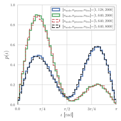
Figure 15: We show the marginal posterior distribution for the inclination angle and its dependence on the number of processes used to parallelize the nested sampling algorithm for one of the representative events: GW190727_060333. Here $n_{\rm node}$, $n_{\rm process}$ and $n_{\rm live}$ denote the number of nodes, processes and live points used in dynesty respectively. The details are in Appendix A.

parallel-bilby uses a parallelized nested sampling algorithm implemented in dynesty Speagle (2020), which parallelizes the step of drawing prior samples to update the live points at each iteration. After live points are updated, the prior volume is constrained to lie within a bounding ellipse containing the new live points, shrinking the prior volume that needs to be sampled at subsequent iterations. In contrast, at each iteration of serial nested sampling, only one prior sample is drawn at a time, and a single live point is updated. The differences in how live points are updated affect how bounding ellipses are drawn at each iteration. In practice, we find the parallel variant can prematurely exclude regions of the prior with reasonable posterior support and becomes problematic whenever the number of live-points-per-process becomes too low.

As the number of live-points-per-process increases, the posteriors converge to a unique distribution. Unfortunately, it is not known ahead of time what this number should be. We empirically determine the correct number by randomly selecting five events and systematically varying this value, finding about 16 live-points-per-process is sufficient.

Fig. 15 shows the posterior’s dependence as the number of live-points-per-process is varied for one of the representative events GW190727_060333. We consider computations carried out with 640 processes on 1 node (green solid curve) and five nodes (red dashed curve), which give nearly identical posteriors as we would expect based on how parallel-bilby’s parallelization is carried out. For an identical setup using 1 node and 128 processes (blue solid curve), we infer a different posterior distribution, which demonstrates the parallelized sampler’s dependence on the number of processes used. We further show “convergence” of the posterior with live-points-per-process. We first use 640 processes distributed across 5 nodes and set $n_{\rm live}=2000$. This gives about 3 live-points-per-process and the resulting posteriors are shown as the red dashed curve. We increase the number of live-points-per-process by either (i) increasing the total number of live points to 8000 (black dashed curve) or (ii) decreasing the number of processes to 128 (blue solid curve). The blue and black curves visually agree, indicating that the number of live-points-per-process is sufficiently large for this problem. Increasing the number of live-points-per-process further still results in posteriors visually identical to the (already converged) blue and black.

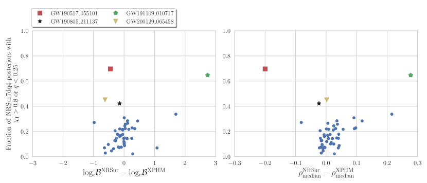
Figure 16: Fraction of NRSur7dq4 posteriors with either $\chi_{1}>0.8$ or $q<1/4$ as a function of the differences in the recovered log Bayes factors (left panel) and the median SNR (right panel) between the NRSur7dq4 (referred to as ‘NRSur’) and IMRPhenomXPHM models (referred to as ‘XPHM’) for all 47 events considered in this work. The events with a fraction $>0.4$ are highlighted. Further details are given in Section V and Appendix  B.1.

Appendix B Understanding the outliers and correlations in model-selection diagnostics

In Sec. V we noted that while there is no outright strong preference for either NRSur7dq4 or IMRPhenomXPHM when considering log Bayes factors or the SNR, the data seems to show a mild preference for NRSur7dq4 over IMRPhenomXPHM. In this appendix, we explore possible explanations for trends and outliers found while performing the model selection.

B.1 Impact due to model extrapolation

The NRSur7dq4 model has been trained on a parameter domain defined by $q\geq 1/4$ and $\chi_{1},\chi_{2}\leq 0.8$, yet throughout this paper, we have used it over the expanded region $q\geq 1/6$ and $\chi_{1},\chi_{2}\leq 0.99$ (see Sec.II.5). We note, however, that IMRPhenomXPHM is also not well calibrated the $q<1/4$ or $\chi_{1}>0.8$ region, and wherever comparisons to NR are possible, NRSur7dq4 is more accurate than existing waveform models Varma et al. (2019a, 2022b); Walker et al. (2023).

To investigate the possibility that the extrapolated model may produce inaccurate waveforms, we compute the fraction of NRSur7dq4 posteriors that require extrapolation in either the mass ratio or the primary spin magnitude - i.e. $q<1/4$ or $\chi_{1}>0.8$, and plot this fraction in Fig.16 as a function of the differences in the log Bayes factor (left panel) and the median SNR (right panel) between NRSur7dq4 and IMRPhenomXPHM for all 47 events considered. For the events where this fraction is relatively small ($<0.4$), we find a mild correlation where NRSur7dq4 is doing better than IMRPhenomXPHM with increasing fractions. For more extreme events (where the fraction is above 0.4 – these are highlighted in Fig.16), there is no clear correlation, and with only 4 events its challenging to say anything meaningful. Synthetic NR injection studies could be used to systematically explore model fidelity in these extreme regions of parameter space.

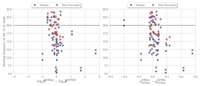
Figure 17: Median (blue circles) and 95th percentile (red crosses) values of the starting frequency of the $(3,3)$ mode of NRSur7dq4 as a function of the differences in the recovered log Bayes factors (left panel) and the median SNR (right panel) between NRSur7dq4 (referred to as ‘NRSur’) and IMRPhenomXPHM models (referred to as ‘XPHM’) for all 47 events considered in this work. Black dashed lines indicate the low frequency cutoff ($f_{\rm low}=20$ Hz) used for the overlap integral. Further details are given in Section V and Appendix  B.2.

B.2 Impact due to model duration

Another possibility is that the NRSur7dq4 model’s limited length causes it to miss some of the higher mode content near $f_{\rm low}=20$ Hz, resulting in a smaller Bayes Factor or SNR for some events.

As explained in Sec.II.6, we use $f_{\rm low}=20$ Hz for the overlap integral, and our NRSur7dq4 evaluations return the full length of the surrogate (about 20 orbits). Given this length restriction, the $(2,2)$ mode for a $M_{{\rm det}}\sim 60M_{\odot}$ BBH system will start at 20 Hz Varma et al. (2019a). This means the higher harmonics will start at multiples of this frequency – for example, the next most important harmonic, the $(3,3)$ mode, will start at 30 Hz. And in general, if the $(2,2)$ mode’s starting frequency is $f_{22}$ the initial frequency of the $(\ell,m)$ waveform is $m/2\times f_{22}$ Hz.

By using the full length of the surrogate, the (2,2) mode is guaranteed to start below $20$ Hz (for $M_{{\rm det}}\gtrsim 60M_{\odot}$), while the higher harmonics with $m>2$ may start above $20$ Hz. Here, we consider if the missing lower frequency content of certain subdominant modes could impact the Bayes Factor and/or the SNR recovered by the surrogate.

To investigate this possibility, for each event, we randomly choose 5000 samples from the NRSur7dq4 posteriors and compute the starting frequency of the $(3,3)$ mode for the NRSur7dq4 model in the co-precessing frame. Figure 17 shows the median and 95 percentile values of the $(3,3)$ mode starting frequency as a function of the differences in the log Bayes factor (left panel) and the median SNR (right panel) between NRSur7dq4 and IMRPhenomXPHM for all 47 events considered. We find no clear correlations suggesting that any missing low-frequency content in the higher harmonics of NRSur7dq4 may not be the cause for the IMRPhenomXPHM model recovering a higher SNR for GW190517_055101 and a higher Bayes factor for GW190706_222641.

While there could be numerous other causes, another possibility worth noting is that noise fluctuations can also cause the data to prefer one model over another. Determining this will require more observations and/or careful NR synthetic injection studies in realistic noise. As detector sensitivity improves and the number of events increases, comparisons like Figs. 9, 16 and 17 can help determine which waveform models best describe the observed data.

References

References

- Harry (2010) Gregory M. Harry (LIGO Scientific), “Advanced LIGO: The next generation of gravitational wave detectors,” Class. Quant. Grav. 27, 084006 (2010).
- Acernese et al. (2015) F. Acernese et al. (VIRGO), “Advanced Virgo: a second-generation interferometric gravitational wave detector,” Class. Quant. Grav. 32, 024001 (2015), arXiv:1408.3978 [gr-qc] .
- Abbott et al. (2019a) B. P. Abbott et al. (LIGO Scientific, Virgo), “GWTC-1: A Gravitational-Wave Transient Catalog of Compact Binary Mergers Observed by LIGO and Virgo during the First and Second Observing Runs,” Phys. Rev. X 9, 031040 (2019a), arXiv:1811.12907 [astro-ph.HE] .
- Abbott et al. (2021a) R. Abbott et al. (LIGO Scientific, Virgo), “GWTC-2: Compact Binary Coalescences Observed by LIGO and Virgo During the First Half of the Third Observing Run,” Phys. Rev. X 11, 021053 (2021a), arXiv:2010.14527 [gr-qc] .
- Abbott et al. (2021b) R. Abbott et al. (LIGO Scientific, VIRGO), “GWTC-2.1: Deep Extended Catalog of Compact Binary Coalescences Observed by LIGO and Virgo During the First Half of the Third Observing Run,” (2021b), arXiv:2108.01045 [gr-qc] .
- Abbott et al. (2021c) R. Abbott et al. (LIGO Scientific, VIRGO, KAGRA), “GWTC-3: Compact Binary Coalescences Observed by LIGO and Virgo During the Second Part of the Third Observing Run,” (2021c), arXiv:2111.03606 [gr-qc] .
- Akutsu et al. (2021) T. Akutsu et al. (KAGRA), “Overview of KAGRA: Detector design and construction history,” PTEP 2021, 05A101 (2021), arXiv:2005.05574 [physics.ins-det] .
- Venumadhav et al. (2020) Tejaswi Venumadhav, Barak Zackay, Javier Roulet, Liang Dai, and Matias Zaldarriaga, “New binary black hole mergers in the second observing run of Advanced LIGO and Advanced Virgo,” Phys. Rev. D 101, 083030 (2020), arXiv:1904.07214 [astro-ph.HE] .
- Nitz et al. (2019) Alexander H. Nitz, Collin Capano, Alex B. Nielsen, Steven Reyes, Rebecca White, Duncan A. Brown, and Badri Krishnan, “1-OGC: The first open gravitational-wave catalog of binary mergers from analysis of public Advanced LIGO data,” Astrophys. J. 872, 195 (2019), arXiv:1811.01921 [gr-qc] .
- Nitz et al. (2020) Alexander H. Nitz, Thomas Dent, Gareth S. Davies, Sumit Kumar, Collin D. Capano, Ian Harry, Simone Mozzon, Laura Nuttall, Andrew Lundgren, and Márton Tápai, “2-OGC: Open Gravitational-wave Catalog of binary mergers from analysis of public Advanced LIGO and Virgo data,” Astrophys. J. 891, 123 (2020), arXiv:1910.05331 [astro-ph.HE] .
- Nitz et al. (2021) Alexander H. Nitz, Collin D. Capano, Sumit Kumar, Yi-Fan Wang, Shilpa Kastha, Marlin Schäfer, Rahul Dhurkunde, and Miriam Cabero, “3-OGC: Catalog of Gravitational Waves from Compact-binary Mergers,” Astrophys. J. 922, 76 (2021), arXiv:2105.09151 [astro-ph.HE] .
- Fishbach et al. (2017) Maya Fishbach, Daniel E. Holz, and Ben Farr, “Are LIGO’s Black Holes Made From Smaller Black Holes?” Astrophys. J. Lett. 840, L24 (2017), arXiv:1703.06869 [astro-ph.HE] .
- Wysocki et al. (2019) Daniel Wysocki, Jacob Lange, and Richard O’Shaughnessy, “Reconstructing phenomenological distributions of compact binaries via gravitational wave observations,” Phys. Rev. D 100, 043012 (2019), arXiv:1805.06442 [gr-qc] .
- Abbott et al. (2019b) B. P. Abbott et al. (LIGO Scientific, Virgo), “Binary Black Hole Population Properties Inferred from the First and Second Observing Runs of Advanced LIGO and Advanced Virgo,” Astrophys. J. Lett. 882, L24 (2019b), arXiv:1811.12940 [astro-ph.HE] .
- Roulet et al. (2020) Javier Roulet, Tejaswi Venumadhav, Barak Zackay, Liang Dai, and Matias Zaldarriaga, “Binary Black Hole Mergers from LIGO/Virgo O1 and O2: Population Inference Combining Confident and Marginal Events,” Phys. Rev. D 102, 123022 (2020), arXiv:2008.07014 [astro-ph.HE] .
- Abbott et al. (2021d) R. Abbott et al. (LIGO Scientific, VIRGO, KAGRA), “The population of merging compact binaries inferred using gravitational waves through GWTC-3,” (2021d), arXiv:2111.03634 [astro-ph.HE] .
- van Son et al. (2022) L. A. C. van Son, S. E. de Mink, M. Renzo, S. Justham, E. Zapartas, K. Breivik, T. Callister, W. M. Farr, and C. Conroy, “No Peaks without Valleys: The Stable Mass Transfer Channel for Gravitational-wave Sources in Light of the Neutron Star–Black Hole Mass Gap,” Astrophys. J. 940, 184 (2022), arXiv:2209.13609 [astro-ph.HE] .
- Payne and Thrane (2023) Ethan Payne and Eric Thrane, “Model exploration in gravitational-wave astronomy with the maximum population likelihood,” Phys. Rev. Res. 5, 023013 (2023), arXiv:2210.11641 [astro-ph.IM] .
- Doctor et al. (2020) Z. Doctor, D. Wysocki, R. O’Shaughnessy, D. E. Holz, and B. Farr, “Black Hole Coagulation: Modeling Hierarchical Mergers in Black Hole Populations,” Astrophys. J. 893, 35 (2020), arXiv:1911.04424 [astro-ph.HE] .
- Fishbach et al. (2021) Maya Fishbach, Zoheyr Doctor, Thomas Callister, Bruce Edelman, Jiani Ye, Reed Essick, Will M. Farr, Ben Farr, and Daniel E. Holz, “When Are LIGO/Virgo’s Big Black Hole Mergers?” Astrophys. J. 912, 98 (2021), arXiv:2101.07699 [astro-ph.HE] .
- Stevenson et al. (2015) Simon Stevenson, Frank Ohme, and Stephen Fairhurst, “Distinguishing compact binary population synthesis models using gravitational-wave observations of coalescing binary black holes,” Astrophys. J. 810, 58 (2015), arXiv:1504.07802 [astro-ph.HE] .
- Abbott et al. (2016a) B. P. Abbott et al. (LIGO Scientific, Virgo), “Astrophysical Implications of the Binary Black-Hole Merger GW150914,” Astrophys. J. Lett. 818, L22 (2016a), arXiv:1602.03846 [astro-ph.HE] .
- Zevin et al. (2017) Michael Zevin, Chris Pankow, Carl L. Rodriguez, Laura Sampson, Eve Chase, Vassiliki Kalogera, and Frederic A. Rasio, “Constraining Formation Models of Binary Black Holes with Gravitational-Wave Observations,” Astrophys. J. 846, 82 (2017), arXiv:1704.07379 [astro-ph.HE] .
- Abbott et al. (2017a) B. P. Abbott et al. (LIGO Scientific, Virgo), “On the Progenitor of Binary Neutron Star Merger GW170817,” Astrophys. J. Lett. 850, L40 (2017a), arXiv:1710.05838 [astro-ph.HE] .
- Abbott et al. (2018) B. P. Abbott et al. (LIGO Scientific, Virgo), “GW170817: Measurements of neutron star radii and equation of state,” Phys. Rev. Lett. 121, 161101 (2018), arXiv:1805.11581 [gr-qc] .
- Most et al. (2018) Elias R. Most, Lukas R. Weih, Luciano Rezzolla, and Jürgen Schaffner-Bielich, “New constraints on radii and tidal deformabilities of neutron stars from GW170817,” Phys. Rev. Lett. 120, 261103 (2018), arXiv:1803.00549 [gr-qc] .
- Essick et al. (2020) Reed Essick, Philippe Landry, and Daniel E. Holz, “Nonparametric Inference of Neutron Star Composition, Equation of State, and Maximum Mass with GW170817,” Phys. Rev. D 101, 063007 (2020), arXiv:1910.09740 [astro-ph.HE] .
- Abbott et al. (2020a) Benjamin P Abbott et al. (LIGO Scientific, Virgo), “Model comparison from LIGO–Virgo data on GW170817’s binary components and consequences for the merger remnant,” Class. Quant. Grav. 37, 045006 (2020a), arXiv:1908.01012 [gr-qc] .
- Yunes and Siemens (2013) Nicolás Yunes and Xavier Siemens, “Gravitational-Wave Tests of General Relativity with Ground-Based Detectors and Pulsar Timing-Arrays,” Living Rev. Rel. 16, 9 (2013), arXiv:1304.3473 [gr-qc] .
- Carson and Yagi (2019) Zack Carson and Kent Yagi, “Parameterized and Consistency Tests of Gravity with GravitationalWaves: Current and Future,” MDPI Proc. 17, 5 (2019), arXiv:1908.07103 [gr-qc] .
- Abbott et al. (2016b) B. P. Abbott et al. (LIGO Scientific, Virgo), “Tests of general relativity with GW150914,” Phys. Rev. Lett. 116, 221101 (2016b), [Erratum: Phys.Rev.Lett. 121, 129902 (2018)], arXiv:1602.03841 [gr-qc] .
- Abbott et al. (2021e) R. Abbott et al. (LIGO Scientific, Virgo), “Tests of general relativity with binary black holes from the second LIGO-Virgo gravitational-wave transient catalog,” Phys. Rev. D 103, 122002 (2021e), arXiv:2010.14529 [gr-qc] .
- Abbott et al. (2019c) B. P. Abbott et al. (LIGO Scientific, Virgo), “Tests of General Relativity with the Binary Black Hole Signals from the LIGO-Virgo Catalog GWTC-1,” Phys. Rev. D 100, 104036 (2019c), arXiv:1903.04467 [gr-qc] .
- Barausse et al. (2015) Enrico Barausse, Vitor Cardoso, and Paolo Pani, “Environmental Effects for Gravitational-wave Astrophysics,” J. Phys. Conf. Ser. 610, 012044 (2015), arXiv:1404.7140 [astro-ph.CO] .
- Abbott et al. (2017b) B. P. Abbott et al. (LIGO Scientific, Virgo, 1M2H, Dark Energy Camera GW-E, DES, DLT40, Las Cumbres Observatory, VINROUGE, MASTER), “A gravitational-wave standard siren measurement of the Hubble constant,” Nature 551, 85–88 (2017b), arXiv:1710.05835 [astro-ph.CO] .
- Abbott et al. (2021f) B. P. Abbott et al. (LIGO Scientific, Virgo), “A Gravitational-wave Measurement of the Hubble Constant Following the Second Observing Run of Advanced LIGO and Virgo,” Astrophys. J. 909, 218 (2021f), arXiv:1908.06060 [astro-ph.CO] .
- Cantiello et al. (2018) Michele Cantiello et al., “A Precise Distance to the Host Galaxy of the Binary Neutron Star Merger GW170817 Using Surface Brightness Fluctuations,” Astrophys. J. Lett. 854, L31 (2018), arXiv:1801.06080 [astro-ph.GA] .
- Husa et al. (2016) Sascha Husa, Sebastian Khan, Mark Hannam, Michael Pürrer, Frank Ohme, Xisco Jiménez Forteza, and Alejandro Bohé, “Frequency-domain gravitational waves from nonprecessing black-hole binaries. I. New numerical waveforms and anatomy of the signal,” Phys. Rev. D 93, 044006 (2016), arXiv:1508.07250 [gr-qc] .
- Khan et al. (2016) Sebastian Khan, Sascha Husa, Mark Hannam, Frank Ohme, Michael Pürrer, Xisco Jiménez Forteza, and Alejandro Bohé, “Frequency-domain gravitational waves from nonprecessing black-hole binaries. II. A phenomenological model for the advanced detector era,” Phys. Rev. D 93, 044007 (2016), arXiv:1508.07253 [gr-qc] .
- London et al. (2018) Lionel London, Sebastian Khan, Edward Fauchon-Jones, Cecilio García, Mark Hannam, Sascha Husa, Xisco Jiménez-Forteza, Chinmay Kalaghatgi, Frank Ohme, and Francesco Pannarale, “First higher-multipole model of gravitational waves from spinning and coalescing black-hole binaries,” Phys. Rev. Lett. 120, 161102 (2018), arXiv:1708.00404 [gr-qc] .
- Khan et al. (2019) Sebastian Khan, Katerina Chatziioannou, Mark Hannam, and Frank Ohme, “Phenomenological model for the gravitational-wave signal from precessing binary black holes with two-spin effects,” Phys. Rev. D 100, 024059 (2019), arXiv:1809.10113 [gr-qc] .
- Hannam et al. (2014a) Mark Hannam, Patricia Schmidt, Alejandro Bohé, Leïla Haegel, Sascha Husa, Frank Ohme, Geraint Pratten, and Michael Pürrer, “Simple Model of Complete Precessing Black-Hole-Binary Gravitational Waveforms,” Phys. Rev. Lett. 113, 151101 (2014a), arXiv:1308.3271 [gr-qc] .
- Khan et al. (2020) Sebastian Khan, Frank Ohme, Katerina Chatziioannou, and Mark Hannam, “Including higher order multipoles in gravitational-wave models for precessing binary black holes,” Phys. Rev. D 101, 024056 (2020), arXiv:1911.06050 [gr-qc] .
- Pratten et al. (2021) Geraint Pratten et al., “Computationally efficient models for the dominant and subdominant harmonic modes of precessing binary black holes,” Phys. Rev. D 103, 104056 (2021), arXiv:2004.06503 [gr-qc] .
- Estellés et al. (2021) Héctor Estellés, Antoni Ramos-Buades, Sascha Husa, Cecilio García-Quirós, Marta Colleoni, Leïla Haegel, and Rafel Jaume, “Phenomenological time domain model for dominant quadrupole gravitational wave signal of coalescing binary black holes,” Phys. Rev. D 103, 124060 (2021), arXiv:2004.08302 [gr-qc] .
- Estellés et al. (2022a) Héctor Estellés, Sascha Husa, Marta Colleoni, David Keitel, Maite Mateu-Lucena, Cecilio García-Quirós, Antoni Ramos-Buades, and Angela Borchers, “Time-domain phenomenological model of gravitational-wave subdominant harmonics for quasicircular nonprecessing binary black hole coalescences,” Phys. Rev. D 105, 084039 (2022a), arXiv:2012.11923 [gr-qc] .
- Estellés et al. (2022b) Héctor Estellés, Marta Colleoni, Cecilio García-Quirós, Sascha Husa, David Keitel, Maite Mateu-Lucena, Maria de Lluc Planas, and Antoni Ramos-Buades, “New twists in compact binary waveform modeling: A fast time-domain model for precession,” Phys. Rev. D 105, 084040 (2022b), arXiv:2105.05872 [gr-qc] .
- Hamilton et al. (2021) Eleanor Hamilton, Lionel London, Jonathan E. Thompson, Edward Fauchon-Jones, Mark Hannam, Chinmay Kalaghatgi, Sebastian Khan, Francesco Pannarale, and Alex Vano-Vinuales, “Model of gravitational waves from precessing black-hole binaries through merger and ringdown,” Phys. Rev. D 104, 124027 (2021), arXiv:2107.08876 [gr-qc] .
- Bohé et al. (2017) Alejandro Bohé et al., “Improved effective-one-body model of spinning, nonprecessing binary black holes for the era of gravitational-wave astrophysics with advanced detectors,” Phys. Rev. D 95, 044028 (2017), arXiv:1611.03703 [gr-qc] .
- Cotesta et al. (2018a) Roberto Cotesta, Alessandra Buonanno, Alejandro Bohé, Andrea Taracchini, Ian Hinder, and Serguei Ossokine, “Enriching the Symphony of Gravitational Waves from Binary Black Holes by Tuning Higher Harmonics,” Phys. Rev. D 98, 084028 (2018a), arXiv:1803.10701 [gr-qc] .
- Cotesta et al. (2020) Roberto Cotesta, Sylvain Marsat, and Michael Pürrer, “Frequency domain reduced order model of aligned-spin effective-one-body waveforms with higher-order modes,” Phys. Rev. D 101, 124040 (2020), arXiv:2003.12079 [gr-qc] .
- Pan et al. (2014a) Yi Pan, Alessandra Buonanno, Andrea Taracchini, Lawrence E. Kidder, Abdul H. Mroué, Harald P. Pfeiffer, Mark A. Scheel, and Béla Szilágyi, “Inspiral-merger-ringdown waveforms of spinning, precessing black-hole binaries in the effective-one-body formalism,” Phys. Rev. D 89, 084006 (2014a), arXiv:1307.6232 [gr-qc] .
- Babak et al. (2017a) Stanislav Babak, Andrea Taracchini, and Alessandra Buonanno, “Validating the effective-one-body model of spinning, precessing binary black holes against numerical relativity,” Phys. Rev. D 95, 024010 (2017a), arXiv:1607.05661 [gr-qc] .
- Ossokine et al. (2020) Serguei Ossokine et al., “Multipolar Effective-One-Body Waveforms for Precessing Binary Black Holes: Construction and Validation,” Phys. Rev. D 102, 044055 (2020), arXiv:2004.09442 [gr-qc] .
- Damour and Nagar (2014) Thibault Damour and Alessandro Nagar, “New effective-one-body description of coalescing nonprecessing spinning black-hole binaries,” Phys. Rev. D 90, 044018 (2014), arXiv:1406.6913 [gr-qc] .
- Nagar et al. (2020a) Alessandro Nagar, Geraint Pratten, Gunnar Riemenschneider, and Rossella Gamba, “Multipolar effective one body model for nonspinning black hole binaries,” Phys. Rev. D 101, 024041 (2020a), arXiv:1904.09550 [gr-qc] .
- Nagar et al. (2020b) Alessandro Nagar, Gunnar Riemenschneider, Geraint Pratten, Piero Rettegno, and Francesco Messina, “Multipolar effective one body waveform model for spin-aligned black hole binaries,” Phys. Rev. D 102, 024077 (2020b), arXiv:2001.09082 [gr-qc] .
- Riemenschneider et al. (2021) Gunnar Riemenschneider, Piero Rettegno, Matteo Breschi, Angelica Albertini, Rossella Gamba, Sebastiano Bernuzzi, and Alessandro Nagar, “Assessment of consistent next-to-quasicircular corrections and postadiabatic approximation in effective-one-body multipolar waveforms for binary black hole coalescences,” Phys. Rev. D 104, 104045 (2021), arXiv:2104.07533 [gr-qc] .
- Khalil et al. (2023) Mohammed Khalil, Alessandra Buonanno, Hector Estelles, Deyan P. Mihaylov, Serguei Ossokine, Lorenzo Pompili, and Antoni Ramos-Buades, “Theoretical groundwork supporting the precessing-spin two-body dynamics of the effective-one-body waveform models SEOBNRv5,” (2023), arXiv:2303.18143 [gr-qc] .
- Pompili et al. (2023) Lorenzo Pompili et al., “Laying the foundation of the effective-one-body waveform models SEOBNRv5: improved accuracy and efficiency for spinning non-precessing binary black holes,” (2023), arXiv:2303.18039 [gr-qc] .
- Ramos-Buades et al. (2023) Antoni Ramos-Buades, Alessandra Buonanno, Héctor Estellés, Mohammed Khalil, Deyan P. Mihaylov, Serguei Ossokine, Lorenzo Pompili, and Mahlet Shiferaw, “SEOBNRv5PHM: Next generation of accurate and efficient multipolar precessing-spin effective-one-body waveforms for binary black holes,” (2023), arXiv:2303.18046 [gr-qc] .
- van de Meent et al. (2023) Maarten van de Meent, Alessandra Buonanno, Deyan P. Mihaylov, Serguei Ossokine, Lorenzo Pompili, Niels Warburton, Adam Pound, Barry Wardell, Leanne Durkan, and Jeremy Miller, “Enhancing the SEOBNRv5 effective-one-body waveform model with second-order gravitational self-force fluxes,” (2023), arXiv:2303.18026 [gr-qc] .
- Blackman et al. (2015) Jonathan Blackman, Scott E. Field, Chad R. Galley, Béla Szilágyi, Mark A. Scheel, Manuel Tiglio, and Daniel A. Hemberger, “Fast and Accurate Prediction of Numerical Relativity Waveforms from Binary Black Hole Coalescences Using Surrogate Models,” Phys. Rev. Lett. 115, 121102 (2015), arXiv:1502.07758 [gr-qc] .
- Blackman et al. (2017a) Jonathan Blackman, Scott E. Field, Mark A. Scheel, Chad R. Galley, Daniel A. Hemberger, Patricia Schmidt, and Rory Smith, “A Surrogate Model of Gravitational Waveforms from Numerical Relativity Simulations of Precessing Binary Black Hole Mergers,” Phys. Rev. D 95, 104023 (2017a), arXiv:1701.00550 [gr-qc] .
- Blackman et al. (2017b) Jonathan Blackman, Scott E. Field, Mark A. Scheel, Chad R. Galley, Christian D. Ott, Michael Boyle, Lawrence E. Kidder, Harald P. Pfeiffer, and Béla Szilágyi, “Numerical relativity waveform surrogate model for generically precessing binary black hole mergers,” Phys. Rev. D 96, 024058 (2017b), arXiv:1705.07089 [gr-qc] .
- Varma et al. (2019a) Vijay Varma, Scott E. Field, Mark A. Scheel, Jonathan Blackman, Davide Gerosa, Leo C. Stein, Lawrence E. Kidder, and Harald P. Pfeiffer, “Surrogate models for precessing binary black hole simulations with unequal masses,” Phys. Rev. Research. 1, 033015 (2019a), arXiv:1905.09300 [gr-qc] .
- Varma et al. (2019b) Vijay Varma, Scott E. Field, Mark A. Scheel, Jonathan Blackman, Lawrence E. Kidder, and Harald P. Pfeiffer, “Surrogate model of hybridized numerical relativity binary black hole waveforms,” Phys. Rev. D 99, 064045 (2019b), arXiv:1812.07865 [gr-qc] .
- Islam et al. (2021a) Tousif Islam, Vijay Varma, Jackie Lodman, Scott E. Field, Gaurav Khanna, Mark A. Scheel, Harald P. Pfeiffer, Davide Gerosa, and Lawrence E. Kidder, “Eccentric binary black hole surrogate models for the gravitational waveform and remnant properties: comparable mass, nonspinning case,” Phys. Rev. D 103, 064022 (2021a), arXiv:2101.11798 [gr-qc] .
- Kumar et al. (2019) Prayush Kumar, Jonathan Blackman, Scott E. Field, Mark Scheel, Chad R. Galley, Michael Boyle, Lawrence E. Kidder, Harald P. Pfeiffer, Bela Szilagyi, and Saul A. Teukolsky, “Constraining the parameters of GW150914 and GW170104 with numerical relativity surrogates,” Phys. Rev. D 99, 124005 (2019), arXiv:1808.08004 [gr-qc] .
- Islam et al. (2021b) Tousif Islam, Scott E. Field, Carl-Johan Haster, and Rory Smith, “Improved analysis of GW190412 with a precessing numerical relativity surrogate waveform model,” Phys. Rev. D 103, 104027 (2021b), arXiv:2010.04848 [gr-qc] .
- Varma et al. (2022a) Vijay Varma, Maximiliano Isi, Sylvia Biscoveanu, Will M. Farr, and Salvatore Vitale, “Measuring binary black hole orbital-plane spin orientations,” Phys. Rev. D 105, 024045 (2022a), arXiv:2107.09692 [astro-ph.HE] .
- Abbott et al. (2020b) R. Abbott et al. (LIGO Scientific, Virgo), “Properties and Astrophysical Implications of the 150 M⊙ Binary Black Hole Merger GW190521,” Astrophys. J. Lett. 900, L13 (2020b), arXiv:2009.01190 [astro-ph.HE] .
- Varma et al. (2022b) Vijay Varma, Sylvia Biscoveanu, Tousif Islam, Feroz H. Shaik, Carl-Johan Haster, Maximiliano Isi, Will M. Farr, Scott E. Field, and Salvatore Vitale, “Evidence of Large Recoil Velocity from a Black Hole Merger Signal,” Phys. Rev. Lett. 128, 191102 (2022b), arXiv:2201.01302 [astro-ph.HE] .
- Collaboration and Collaboration (2022a) LIGO Scientific Collaboration and Virgo Collaboration, “GWTC-2.1: Deep Extended Catalog of Compact Binary Coalescences Observed by LIGO and Virgo During the First Half of the Third Observing Run - Parameter Estimation Data Release,” https://zenodo.org/record/6513631 (2022a).
- Collaboration et al. (2021a) LIGO Scientific Collaboration, Virgo Collaboration, and KAGRA Collaboration, “GWTC-3: Compact Binary Coalescences Observed by LIGO and Virgo During the Second Part of the Third Observing Run — Parameter estimation data release,” https://zenodo.org/record/5546663 (2021a).
- T. et al. (2023) Islam T., Vajpeyi A., Shaik F., Haster C., Varma V., Field S., Lange J., O’Shaughnessy R., and Smith R., “NRSurrogate Catalog Website,” https://nrsur-catalog.github.io/NRSurCat-1, https://doi.org/10.5281/zenodo.8115310 (2023).
- Romero-Shaw et al. (2020) I. M. Romero-Shaw et al., “Bayesian inference for compact binary coalescences with bilby: validation and application to the first LIGO–Virgo gravitational-wave transient catalogue,” Mon. Not. Roy. Astron. Soc. 499, 3295–3319 (2020), arXiv:2006.00714 [astro-ph.IM] .
- Field et al. (2014) Scott E. Field, Chad R. Galley, Jan S. Hesthaven, Jason Kaye, and Manuel Tiglio, “Fast prediction and evaluation of gravitational waveforms using surrogate models,” Phys. Rev. X 4, 031006 (2014), arXiv:1308.3565 [gr-qc] .
- Field et al. (2011) S. E. Field, C. R. Galley, F. Herrmann, J. S. Hesthaven, E. Ochsner, and M. Tiglio, “Reduced basis catalogs for gravitational wave templates,” Phys. Rev. Lett. 106, 221102 (2011), arXiv:1101.3765 [gr-qc] .
- Walker et al. (2023) Marissa Walker, Vijay Varma, Geoffrey Lovelace, and Mark A. Scheel, “Numerical-relativity surrogate modeling with nearly extremal black-hole spins,” Class. Quant. Grav. 40, 055003 (2023), arXiv:2208.02927 [gr-qc] .
- García-Quirós et al. (2020) Cecilio García-Quirós, Marta Colleoni, Sascha Husa, Héctor Estellés, Geraint Pratten, Antoni Ramos-Buades, Maite Mateu-Lucena, and Rafel Jaume, “Multimode frequency-domain model for the gravitational wave signal from nonprecessing black-hole binaries,” Phys. Rev. D 102, 064002 (2020), arXiv:2001.10914 [gr-qc] .
- Pratten et al. (2020) Geraint Pratten, Sascha Husa, Cecilio Garcia-Quiros, Marta Colleoni, Antoni Ramos-Buades, Hector Estelles, and Rafel Jaume, “Setting the cornerstone for a family of models for gravitational waves from compact binaries: The dominant harmonic for nonprecessing quasicircular black holes,” Phys. Rev. D 102, 064001 (2020), arXiv:2001.11412 [gr-qc] .
- Cotesta et al. (2018b) Roberto Cotesta, Alessandra Buonanno, Alejandro Bohé, Andrea Taracchini, Ian Hinder, and Serguei Ossokine, “Enriching the Symphony of Gravitational Waves from Binary Black Holes by Tuning Higher Harmonics,” Phys. Rev. D 98, 084028 (2018b), arXiv:1803.10701 [gr-qc] .
- Varma et al. (2019c) Vijay Varma, Davide Gerosa, Leo C. Stein, François Hébert, and Hao Zhang, “High-accuracy mass, spin, and recoil predictions of generic black-hole merger remnants,” Phys. Rev. Lett. 122, 011101 (2019c), arXiv:1809.09125 [gr-qc] .
- Schmidt et al. (2017) Patricia Schmidt, Ian W. Harry, and Harald P. Pfeiffer, “Numerical Relativity Injection Infrastructure,” (2017), arXiv:1703.01076 [gr-qc] .
- Abbott et al. (2021g) Rich Abbott et al. (LIGO Scientific, Virgo), “Open data from the first and second observing runs of Advanced LIGO and Advanced Virgo,” SoftwareX 13, 100658 (2021g), arXiv:1912.11716 [gr-qc] .
- Collaboration and Collaboration (2022b) LIGO Scientific Collaboration and Virgo Collaboration, “GWTC-2.1: Deep Extended Catalog of Compact Binary Coalescences Observed by LIGO and Virgo During the First Half of the Third Observing Run - Glitch modelling for events,” https://zenodo.org/record/6477076 (2022b).
- Collaboration et al. (2021b) LIGO Scientific Collaboration, Virgo Collaboration, and KAGRA Collaboration, “GWTC-3: Compact Binary Coalescences Observed by LIGO and Virgo During the Second Part of the Third Observing Run — Glitch modelling for events,” https://zenodo.org/record/5546680 (2021b).
- Littenberg and Cornish (2015) Tyson B. Littenberg and Neil J. Cornish, “Bayesian inference for spectral estimation of gravitational wave detector noise,” Phys. Rev. D 91, 084034 (2015), arXiv:1410.3852 [gr-qc] .
- Cornish and Littenberg (2015) Neil J. Cornish and Tyson B. Littenberg, “BayesWave: Bayesian Inference for Gravitational Wave Bursts and Instrument Glitches,” Class. Quant. Grav. 32, 135012 (2015), arXiv:1410.3835 [gr-qc] .
- Chatziioannou et al. (2019) Katerina Chatziioannou, Carl-Johan Haster, Tyson B. Littenberg, Will M. Farr, Sudarshan Ghonge, Margaret Millhouse, James A. Clark, and Neil Cornish, “Noise spectral estimation methods and their impact on gravitational wave measurement of compact binary mergers,” Phys. Rev. D 100, 104004 (2019), arXiv:1907.06540 [gr-qc] .
- Farr W. M. (2014) Littenberg T. Farr W. M., Farr B., “Technical Report LIGO-T1400682, Modelling calibration errors in CBC waveforms,” https://dcc.ligo.org/LIGO-T1400460/public (2014).
- (93) “Glitch model for O3a catalog events,” https://dcc.ligo.org/LIGO-T2000470/public.
- Finn and Chernoff (1993) Lee Samuel Finn and David F. Chernoff, “Observing binary inspiral in gravitational radiation: One interferometer,” Phys. Rev. D 47, 2198–2219 (1993).
- Speagle (2020) Joshua S. Speagle, “dynesty: a dynamic nested sampling package for estimating Bayesian posteriors and evidences,” Mon. Not. Roy. Astron. Soc. 493, 3132–3158 (2020), arXiv:1904.02180 [astro-ph.IM] .
- Smith et al. (2020) Rory J. E. Smith, Gregory Ashton, Avi Vajpeyi, and Colm Talbot, “Massively parallel Bayesian inference for transient gravitational-wave astronomy,” Mon. Not. Roy. Astron. Soc. 498, 4492–4502 (2020), arXiv:1909.11873 [gr-qc] .
- Ashton et al. (2019) Gregory Ashton et al., “BILBY: A user-friendly Bayesian inference library for gravitational-wave astronomy,” Astrophys. J. Suppl. 241, 27 (2019), arXiv:1811.02042 [astro-ph.IM] .
- Skilling (2006a) John Skilling, “Nested sampling for general Bayesian computation,” Bayesian Analysis 1, 833–859 (2006a).
- Abbott et al. (2020c) R. Abbott et al. (LIGO Scientific, Virgo), “GW190521: A Binary Black Hole Merger with a Total Mass of ,” Phys. Rev. Lett. 125, 101102 (2020c), arXiv:2009.01075 [gr-qc] .
- (100) “We use a version of lalsimulation after the SimInspiralFD frequency spacing merge request was accepted,” https://git.ligo.org/lscsoft/lalsuite/merge_requests/1785.
- Ajith et al. (2011) P. Ajith et al., “Inspiral-merger-ringdown waveforms for black-hole binaries with non-precessing spins,” Phys. Rev. Lett. 106, 241101 (2011), arXiv:0909.2867 [gr-qc] .
- Santamaria et al. (2010) L. Santamaria et al., “Matching post-Newtonian and numerical relativity waveforms: systematic errors and a new phenomenological model for non-precessing black hole binaries,” Phys. Rev. D 82, 064016 (2010), arXiv:1005.3306 [gr-qc] .
- Vitale et al. (2017) Salvatore Vitale, Ryan Lynch, Vivien Raymond, Riccardo Sturani, John Veitch, and Philp Graff, “Parameter estimation for heavy binary-black holes with networks of second-generation gravitational-wave detectors,” Phys. Rev. D 95, 064053 (2017), arXiv:1611.01122 [gr-qc] .
- Hannam et al. (2014b) Mark Hannam, Patricia Schmidt, Alejandro Bohé, Leïla Haegel, Sascha Husa, Frank Ohme, Geraint Pratten, and Michael Pürrer, “Simple Model of Complete Precessing Black-Hole-Binary Gravitational Waveforms,” Phys. Rev. Lett. 113, 151101 (2014b), arXiv:1308.3271 [gr-qc] .
- Schmidt et al. (2015) Patricia Schmidt, Frank Ohme, and Mark Hannam, “Towards models of gravitational waveforms from generic binaries II: Modelling precession effects with a single effective precession parameter,” Phys. Rev. D 91, 024043 (2015), arXiv:1408.1810 [gr-qc] .
- Lange et al. (2018) Jacob Lange, Richard O’Shaughnessy, and Monica Rizzo, “Rapid and accurate parameter inference for coalescing, precessing compact binaries,” (2018), arXiv:1805.10457 [gr-qc] .
- Lin (1991) J. Lin, “Divergence measures based on the Shannon entropy,” IEEE Transactions on Information Theory 37, 145–151 (1991).
- Kullback and Leibler (1951) S. Kullback and R. A. Leibler, “On Information and Sufficiency,” The Annals of Mathematical Statistics 22, 79 – 86 (1951).
- Abbott et al. (2016c) Thomas D. Abbott et al. (LIGO Scientific, Virgo), “Improved analysis of GW150914 using a fully spin-precessing waveform Model,” Phys. Rev. X 6, 041014 (2016c), arXiv:1606.01210 [gr-qc] .
- Shaik et al. (2020) Feroz H Shaik, Jacob Lange, Scott E Field, Richard O’Shaughnessy, Vijay Varma, Lawrence E Kidder, Harald P Pfeiffer, and Daniel Wysocki, “Impact of subdominant modes on the interpretation of gravitational-wave signals from heavy binary black hole systems,” Physical Review D 101, 124054 (2020).
- Payne et al. (2019) Ethan Payne, Colm Talbot, and Eric Thrane, “Higher order gravitational-wave modes with likelihood reweighting,” Phys. Rev. D 100, 123017 (2019), arXiv:1905.05477 [astro-ph.IM] .
- Payne et al. (2020) Ethan Payne, Colm Talbot, Paul D. Lasky, Eric Thrane, and Jeffrey S. Kissel, “Gravitational-wave astronomy with a physical calibration model,” Phys. Rev. D 102, 122004 (2020), arXiv:2009.10193 [astro-ph.IM] .
- Mateu-Lucena et al. (2022) Maite Mateu-Lucena, Sascha Husa, Marta Colleoni, Héctor Estellés, Cecilio García-Quirós, David Keitel, Maria de Lluc Planas, and Antoni Ramos-Buades, “Parameter estimation with the current generation of phenomenological waveform models applied to the black hole mergers of GWTC-1,” Mon. Not. Roy. Astron. Soc. 517, 2403–2425 (2022), arXiv:2105.05960 [gr-qc] .
- Abbott et al. (2017c) Benjamin P. Abbott et al. (LIGO Scientific, Virgo), “Effects of waveform model systematics on the interpretation of GW150914,” Class. Quant. Grav. 34, 104002 (2017c), arXiv:1611.07531 [gr-qc] .
- Pan et al. (2014b) Yi Pan, Alessandra Buonanno, Andrea Taracchini, Lawrence E. Kidder, Abdul H. Mroué, Harald P. Pfeiffer, Mark A. Scheel, and Béla Szilágyi, “Inspiral-merger-ringdown waveforms of spinning, precessing black-hole binaries in the effective-one-body formalism,” Phys. Rev. D 89, 084006 (2014b), arXiv:1307.6232 [gr-qc] .
- Taracchini et al. (2014) Andrea Taracchini et al., “Effective-one-body model for black-hole binaries with generic mass ratios and spins,” Phys. Rev. D 89, 061502 (2014), arXiv:1311.2544 [gr-qc] .
- Babak et al. (2017b) Stanislav Babak, Andrea Taracchini, and Alessandra Buonanno, “Validating the effective-one-body model of spinning, precessing binary black holes against numerical relativity,” Phys. Rev. D 95, 024010 (2017b), arXiv:1607.05661 [gr-qc] .
- Veitch et al. (2015) J. Veitch et al., “Parameter estimation for compact binaries with ground-based gravitational-wave observations using the LALInference software library,” Phys. Rev. D 91, 042003 (2015), arXiv:1409.7215 [gr-qc] .
- Abbott et al. (2020d) R. Abbott et al. (LIGO Scientific, Virgo), “Properties and Astrophysical Implications of the 150 M⊙ Binary Black Hole Merger GW190521,” Astrophys. J. Lett. 900, L13 (2020d), arXiv:2009.01190 [astro-ph.HE] .
- Biscoveanu et al. (2021) Sylvia Biscoveanu, Maximiliano Isi, Vijay Varma, and Salvatore Vitale, “Measuring the spins of heavy binary black holes,” Phys. Rev. D 104, 103018 (2021), arXiv:2106.06492 [gr-qc] .
- Estellés et al. (2022c) Héctor Estellés et al., “A Detailed Analysis of GW190521 with Phenomenological Waveform Models,” Astrophys. J. 924, 79 (2022c), arXiv:2105.06360 [gr-qc] .
- Nitz and Capano (2021) Alexander H. Nitz and Collin D. Capano, “GW190521 may be an intermediate mass ratio inspiral,” Astrophys. J. Lett. 907, L9 (2021), arXiv:2010.12558 [astro-ph.HE] .
- Ángel Garrón and Keitel (2023) Ángel Garrón and David Keitel, “Waveform systematics in identifying gravitationally lensed gravitational waves: Posterior overlap method,” (2023), arXiv:2306.12908 [gr-qc] .
- Dax et al. (2023) Maximilian Dax, Stephen R. Green, Jonathan Gair, Michael Pürrer, Jonas Wildberger, Jakob H. Macke, Alessandra Buonanno, and Bernhard Schölkopf, “Neural Importance Sampling for Rapid and Reliable Gravitational-Wave Inference,” Phys. Rev. Lett. 130, 171403 (2023), arXiv:2210.05686 [gr-qc] .
- Dax et al. (2021) Maximilian Dax, Stephen R. Green, Jonathan Gair, Jakob H. Macke, Alessandra Buonanno, and Bernhard Schölkopf, “Real-Time Gravitational Wave Science with Neural Posterior Estimation,” Phys. Rev. Lett. 127, 241103 (2021), arXiv:2106.12594 [gr-qc] .
- Mandel and O’Shaughnessy (2010) Ilya Mandel and Richard O’Shaughnessy, “Compact Binary Coalescences in the Band of Ground-based Gravitational-Wave Detectors,” Class. Quant. Grav. 27, 114007 (2010), arXiv:0912.1074 [astro-ph.HE] .
- Rodriguez et al. (2016) Carl L. Rodriguez, Michael Zevin, Chris Pankow, Vasilliki Kalogera, and Frederic A. Rasio, “Illuminating Black Hole Binary Formation Channels with Spins in Advanced LIGO,” Astrophys. J. Lett. 832, L2 (2016), arXiv:1609.05916 [astro-ph.HE] .
- Payne et al. (2022) Ethan Payne, Sophie Hourihane, Jacob Golomb, Rhiannon Udall, Richard Udall, Derek Davis, and Katerina Chatziioannou, “Curious case of GW200129: Interplay between spin-precession inference and data-quality issues,” Phys. Rev. D 106, 104017 (2022), arXiv:2206.11932 [gr-qc] .
- Davis et al. (2022) D. Davis, T. B. Littenberg, I. M. Romero-Shaw, M. Millhouse, J. McIver, F. Di Renzo, and G. Ashton, “Subtracting glitches from gravitational-wave detector data during the third LIGO-Virgo observing run,” Class. Quant. Grav. 39, 245013 (2022), arXiv:2207.03429 [astro-ph.IM] .
- Abbott et al. (2021h) R. Abbott et al. (LIGO Scientific, VIRGO, KAGRA), “Tests of General Relativity with GWTC-3,” (2021h), arXiv:2112.06861 [gr-qc] .
- Hannam et al. (2022) Mark Hannam et al., “General-relativistic precession in a black-hole binary,” Nature 610, 652–655 (2022), arXiv:2112.11300 [gr-qc] .
- Skilling (2006b) John Skilling, “Nested sampling for general Bayesian computation,” Bayesian Analysis 1, 833 – 859 (2006b).
- Skilling (2004) John Skilling, “Nested Sampling,” in Bayesian Inference and Maximum Entropy Methods in Science and Engineering: 24th International Workshop on Bayesian Inference and Maximum Entropy Methods in Science and Engineering, American Institute of Physics Conference Series, Vol. 735, edited by Rainer Fischer, Roland Preuss, and Udo Von Toussaint (2004) pp. 395–405.
- Koposov et al. (2023) Sergey Koposov, Josh Speagle, Kyle Barbary, Gregory Ashton, Ed Bennett, Johannes Buchner, Carl Scheffler, Ben Cook, Colm Talbot, James Guillochon, and et al., “joshspeagle/dynesty: v2.1.2,” (2023), 10.5281/zenodo.7995596.
- Campanelli et al. (2007) Manuela Campanelli, Carlos O. Lousto, Yosef Zlochower, and David Merritt, “Maximum gravitational recoil,” Phys. Rev. Lett. 98, 231102 (2007), arXiv:gr-qc/0702133 .
- Gonzalez et al. (2007a) J. A. Gonzalez, M. D. Hannam, U. Sperhake, Bernd Bruegmann, and S. Husa, “Supermassive recoil velocities for binary black-hole mergers with antialigned spins,” Phys. Rev. Lett. 98, 231101 (2007a), arXiv:gr-qc/0702052 .
- Lousto and Zlochower (2011) Carlos O. Lousto and Yosef Zlochower, “Hangup Kicks: Still Larger Recoils by Partial Spin/Orbit Alignment of Black-Hole Binaries,” Phys. Rev. Lett. 107, 231102 (2011), arXiv:1108.2009 [gr-qc] .
- Gonzalez et al. (2007b) Jose A. Gonzalez, Ulrich Sperhake, Bernd Bruegmann, Mark Hannam, and Sascha Husa, “Total recoil: The Maximum kick from nonspinning black-hole binary inspiral,” Phys. Rev. Lett. 98, 091101 (2007b), arXiv:gr-qc/0610154 .
- Varma et al. (2020) Vijay Varma, Maximiliano Isi, and Sylvia Biscoveanu, “Extracting the Gravitational Recoil from Black Hole Merger Signals,” Phys. Rev. Lett. 124, 101104 (2020), arXiv:2002.00296 [gr-qc] .
- Varma et al. (2022c) Vijay Varma, Sylvia Biscoveanu, Maximiliano Isi, Will M. Farr, and Salvatore Vitale, “Hints of Spin-Orbit Resonances in the Binary Black Hole Population,” Phys. Rev. Lett. 128, 031101 (2022c), arXiv:2107.09693 [astro-ph.HE] .
- Mahapatra et al. (2021) Parthapratim Mahapatra, Anuradha Gupta, Marc Favata, K. G. Arun, and B. S. Sathyaprakash, “Remnant Black Hole Kicks and Implications for Hierarchical Mergers,” Astrophys. J. Lett. 918, L31 (2021), arXiv:2106.07179 [astro-ph.HE] .
- Calderón Bustillo et al. (2022) Juan Calderón Bustillo, Samson H. W. Leong, and Koustav Chandra, “GW190412: measuring a black-hole recoil direction through higher-order gravitational-wave modes,” (2022), arXiv:2211.03465 [gr-qc] .
- Graham et al. (2020) M.J. Graham et al., “Candidate Electromagnetic Counterpart to the Binary Black Hole Merger Gravitational Wave Event S190521g,” Phys. Rev. Lett. 124, 251102 (2020), arXiv:2006.14122 [astro-ph.HE] .
- Moore and Gerosa (2016) Christopher James Moore and Davide Gerosa, “Black hole kicks as new gravitational wave observables,” (2016).
- Mahapatra et al. (2023) Parthapratim Mahapatra, Marc Favata, and K. G. Arun, “Testing general relativity via direct measurement of black hole kicks,” (2023), arXiv:2308.08319 [gr-qc] .
- Barausse and Rezzolla (2009) Enrico Barausse and Luciano Rezzolla, “Predicting the direction of the final spin from the coalescence of two black holes,” Astrophys. J. Lett. 704, L40–L44 (2009), arXiv:0904.2577 [gr-qc] .
- Hofmann et al. (2016) Fabian Hofmann, Enrico Barausse, and Luciano Rezzolla, “The final spin from binary black holes in quasi-circular orbits,” Astrophys. J. Lett. 825, L19 (2016), arXiv:1605.01938 [gr-qc] .
- Johnson-McDaniel et al. (2016) Nathan K. Johnson-McDaniel, Anuradha Gupta, P Ajith, David Keitel, Ofek Birnholtz, Frank Ohme, and Sascha Husa, Determining the final spin of a binary black hole system including in-plane spins: Method and checks of accuracy, Tech. Rep. LIGO-T1600168 (2016) https://dcc.ligo.org/LIGO-T1600168/public.
- Healy and Lousto (2017) James Healy and Carlos O. Lousto, “Remnant of binary black-hole mergers: New simulations and peak luminosity studies,” Phys. Rev. D95, 024037 (2017), arXiv:1610.09713 [gr-qc] .
- Jiménez-Forteza et al. (2017) Xisco Jiménez-Forteza, David Keitel, Sascha Husa, Mark Hannam, Sebastian Khan, and Michael Pürrer, “Hierarchical data-driven approach to fitting numerical relativity data for nonprecessing binary black holes with an application to final spin and radiated energy,” Phys. Rev. D95, 064024 (2017), arXiv:1611.00332 [gr-qc] .
- Pürrer and Haster (2020) Michael Pürrer and Carl-Johan Haster, “Gravitational waveform accuracy requirements for future ground-based detectors,” Phys. Rev. Res. 2, 023151 (2020), arXiv:1912.10055 [gr-qc] .
- Abbott et al. (2023) R. Abbott et al. (LIGO Scientific, Virgo,, KAGRA, VIRGO), “Constraints on the Cosmic Expansion History from GWTC–3,” Astrophys. J. 949, 76 (2023), arXiv:2111.03604 [astro-ph.CO] .
- (153) Daniel Foreman-Mackey and Avi Vajpeyi, “TESS Atlas,” https://github.com/dfm/tess-atlas.