Flux Correlators and Semiclassics

Eren Firat^a, Alexander Monin^a,b, Riccardo Rattazzi^a, Matthew T. Walters^a,c,d,e

^a Theoretical Particle Physics Laboratory (LPTP), Institute of Physics,
École Polytechnique Fédérale de Lausanne (EPFL), CH-1015 Lausanne, Switzerland

^b Department of Physics and Astronomy,
University of South Carolina, Columbia, SC 29208, USA

^c Department of Theoretical Physics,
Université de Genève, CH-1211 Genève, Switzerland
^d Hamilton Mathematics Institute, School of Mathematics,
Trinity College, Dublin 2, Ireland
^e Maxwell Institute for Mathematical Sciences, Department of Mathematics,
Heriot-Watt University, Edinburgh EH14, UK

We consider correlators for the flux of energy and charge in the background of operators with large global $U(1)$ charge in conformal field theory (CFT). It has recently been shown that the corresponding Euclidean correlators generically admit a semiclassical description in terms of the effective field theory (EFT) for a conformal superfluid. We adapt the semiclassical description to Lorentzian observables and compute the leading large charge behavior of the flux correlators in general $U(1)$ symmetric CFTs. We discuss the regime of validity of the large charge EFT for these Lorentzian observables and the subtleties in extending the EFT approach to subleading corrections. We also consider the Wilson-Fisher fixed point in $d=4-\epsilon$ dimensions, which offers a specific weakly coupled realization of the general setup, where the subleading corrections can be systematically computed without relying on an EFT.

1 Introduction

The fundamental laws of physics, as codified by Quantum Field Theory (QFT), are best deduced by studying the near-vacuum dynamics. The latter consists of processes involving a small number of quanta, like for instance $2\to 2$ transitions. The Standard Model (SM) was indeed constructed on those simple methodological grounds. It is nonetheless awe-inspiring how its very same laws also underlie the vastly more complex macroscopic phenomena one finds in condensed matter, chemistry, or biology.

Key to the variety of macroscopic phenomena and to their effective dynamical laws is, obviously, states involving many quanta and, as such, far from the vacuum. The Standard Model (SM) serves as a perfect example, vividly showcasing the diversity of such states and their often intricate dynamics. In light of this, any situation where the system’s behavior can be calculated, bridging the gap between the few quanta and the many quanta regimes, becomes conceptually intriguing.

As it turns out, an instance of the desired situation is offered by multilegged amplitudes in weakly coupled QFT. Broadly, in a QFT with a weak coupling $\lambda\ll 1$, one finds that the perturbative series for $n$-legged amplitudes is controlled both by $\lambda$ and by $\lambda n$. In practice the dependence on $n$ originates from combinatoric factors in the diagrammatics [2, 3]. For $\lambda n\ll 1$ the standard Feynman diagram expansion works well, but at $\lambda n\gtrsim O(1)$ it breaks down signaling the onset of a new regime. The ranges $\lambda n\ll 1$ and $\lambda n\gg 1$ then naturally and respectively define the few quanta and the many quanta regimes. While these facts were certainly known long before, significant progress on their study was only made in the early 90’s [4, 5, 6, 7, 8, 9]. In particular, focusing on transitions of the type ${\it few}\to n$ for massive scalars near threshold, it was shown that the regime $n\gg 1$ is controlled by a semiclassical expansion [8, 9] around a non-trivial complex (and singular) solution, whose “distance” from the vacuum is controlled by the critical parameter $\lambda n$. While this realization helped sort out crucial structural aspects, the properties of the saddle solution at $\lambda n\gg 1$ proved hard to tackle. Luckily, the computational difficulties have been numerically tackled in a recent remarkable paper [10]. There it was explicitly shown that the probability for the ${\it few}\to n$ transition is exponentially suppressed as $n\to\infty$ for boost factors $\gamma\equiv E/m$ of the particles in the range $1$ to $\sim\!5$. The results of [10] thus represent one example where, for energies ranging from non-relativistic to moderately relativistic, the dynamics across the frontier between less and more is both understood, in terms of a semiclassical expansion, and computed, by numerical methods.

The preceding success story prompts the exploration of other scenarios featuring calculable multilegged amplitudes. Indeed, thanks to recent progress, one such instance is already offered by the large charge regime in Conformal Field Theory [11, 12, 13, 14, 15, 16, 17, 18, 19, 20, 21, 22, 23, 24, 25, 26, 27, 28]. There the number of legs $n$ essentially corresponds to a global $U(1)$ charge $Q$. The main result is that the Euclidean correlators involving the insertion of large-$Q$ operators are described by a semiclassical expansion around a non-trivial solution, controlled by inverse powers of $Q$. When working on the cylinder the solution corresponds to a superfluid state with charge density $J^{0}\sim Q$, in such a way that the behavior at large $Q$ is universally and effectively described by the hydrodynamics of phonons. These results have broad validity and they apply to both weakly coupled models, like Wilson-Fisher models or large $N$ ones, and to generic strongly coupled CFTs.

The weakly coupled cases [16, 17, 18] offer indeed the opportunity to study the behavior of the system for arbitrary $\lambda n$, thus allowing us to follow the dynamics across the few quanta ($\lambda n\ll 1$) and the many quanta ($\lambda n\gg 1$) regimes. One finds that $\lambda n$ crucially controls the gap of non-phononic modes, such that for $\lambda n\gg 1$ the system behaves as a simple generic superfluid at distances larger than $1/\lambda n$ on the cylinder. All these calculations can be carried out analytically, thus illuminating the less to more regime change without the technical complications of the case of multiparticle production.

The simple superfluid behavior that can be explicitly proven in weakly coupled theories is indeed expected at sufficiently large $Q$ for generic CFTs, including strongly coupled ones. This expectation follows from the hypothesis of semiclassicality and from the simplest choice for the symmetry of the saddle solution [12]. Crucially, for generic CFTs the large $Q$ description must be interpreted as an effective one, valid only at lengths larger than the inverse gap of the non-phononic excitations on the cylinder. This regime translates into specific ranges for the conformal cross-ratios of operator positions.

The large charge CFT regime has, so far, been explored in Euclidean signature, or, equivalently, at spacelike separation. The present paper aims to extend the study to inherently Lorentzian observables, which are closer to those that can be directly measured in collider experiments. That would provide a novel (intrinsically ultra-relativistic) situation in which to study the less to more transition, adding to the above mentioned examples.

One natural set of Lorentzian observables for CFTs was presented in [29]: the charge and energy flux resulting from a localized excitation created by a scalar operator. In this work, we consider the same setup as [29], shown in Figure 1, for general CFTs with a global $U(1)$ symmetry, with the local excitation at time $t=0$ created by the lowest-dimension operator $\mathcal{O}_{Q}$ with charge $Q\to\infty$. We can then place a detector a large distance away in order to measure the total charge flux in a given direction resulting from this excitation,

$$\mathcal{Q}(\mathbf{n})\equiv\lim_{r\to\infty}r^{d-2}\int_{0}^{\infty}dt\,n^{i}J^{i}(t,r\mathbf{n}),$$ (1.1)

where $J^{\mu}$ is the conserved current associated with the $U(1)$ symmetry, and the spatial unit vector $\mathbf{n}$ specifies the direction in which we measure the flux. Similarly, we can measure the energy flux

$$\mathcal{E}(\mathbf{n})\equiv\lim_{r\to\infty}r^{d-2}\int_{0}^{\infty}dt\,n^{i}T^{0i}(t,r\mathbf{n}),$$ (1.2)

where $T^{\mu\nu}$ is the stress-energy tensor.

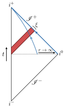
Figure 1: Penrose diagram showing our setup for a spacetime slice of fixed direction $\mathbf{n}$. The operator $\mathcal{O}_{Q}$ creates a localized excitation at time $t=0$, which propagates radially outwards (red band). The resulting charge and energy flux in a given direction are measured by the line operators (1.1) and (1.2), which in the limit $r\to\infty$ become integrals over future null infinity (blue line). The distribution of this flux in time is set by the typical scale $\xi$ of the excitation.

Following [29] we consider a state of the form

$$\mathcal{O}_{Q}(E)\rangle\equiv\int d^{d}x\,e^{-iEx^{0}}e^{-\frac{x_{E}^{2}}{\xi^{2}}}\mathcal{O}_{Q}(x)|0\rangle,$$ (1.3)

where $x_{E}^{2}\equiv\sum_{\mu}(x^{\mu})^{2}$ is a Euclidean norm ensuring the state is normalizable and localized in a region of spacetime where all coordinates are less than $O(\xi)$. In the limit $\xi E\gg 1$ the state approaches a momentum eigenstate, with $P^{\mu}=(E,\vec{0})$. The idea is that the limit $\xi\to\infty$ is taken after the limit $r\to\infty$ in eqs. (1.1) and (1.2).

In such a state, we compute correlators with multiple insertions of the flux operators

$$\langle\mathcal{Q}(\mathbf{n}_{1})\mspace{1.0mu}\cdots\mspace{1.0mu}\mathcal{Q}(\mathbf{n}_{k})\rangle\equiv\frac{\langle\overline{\mathcal{O}}_{Q}(E)\mspace{1.0mu}\mathcal{Q}(\mathbf{n}_{1})\mspace{1.0mu}\cdots\mspace{1.0mu}\mathcal{Q}(\mathbf{n}_{k})\mspace{1.0mu}\mathcal{O}_{Q}(E)\rangle}{\langle\overline{\mathcal{O}}_{Q}(E)\mspace{1.0mu}\mathcal{O}_{Q}(E)\rangle},$$ (1.4)

with an analogous expression for the energy flux. Conceptually, we can think of the excitation created by $\mathcal{O}_{Q}(x)$ as roughly $Q$ charged quanta initially localized at $x$, which propagate outwards and are measured at infinity. By measuring the correlation between charge and energy depositions in different directions, we can determine the makeup and dynamics of these charged quanta, just like in a collider experiment.

The overall normalization of these correlation functions is fixed by Ward identities, but in principle they can otherwise have arbitrary dependence on the angular separations $\cos\theta_{ij}=\mathbf{n}_{i}\cdot\mathbf{n}_{j}$ between the flux operator insertions. For example, we can write the correlator with two charge flux insertions in the general form

$$\langle\mathcal{Q}(\mathbf{n}_{1})\mspace{1.0mu}\mathcal{Q}(\mathbf{n}_{2})\rangle\equiv\frac{Q^{2}}{\Omega^{2}_{d-2}}\big{(}1+h_{Q}(d,\theta)\big{)},$$ (1.5)

where $\Omega_{d-2}\equiv\frac{2\pi^{(d-1)/2}}{\Gamma((d-1)/2)}$ is the area of the celestial sphere, and $\theta\equiv\theta_{12}$. Charge conservation imposes the constraint

$$\int d\Omega_{d-2}\,h_{Q}(d,\theta)=0.$$ (1.6)

For $Q\gg 1$ in a generic CFT in $d$ spacetime dimensions, the EFT results of [11, 12] together with, as we shall argue, an additional hypothesis of smoothness of the 4-point function, imply that $h_{Q}(d,\theta)$ can be expanded in inverse powers of $Q$ as

$$h_{Q}(d,\theta)=h^{(0)}(d,\theta)+\frac{1}{Q^{\alpha}}h^{(1)}(d,\theta)+\ldots$$ (1.7)

To be more precise, within the domain of validity of the EFT of [11, 12], the subleading correction to the 4-point function $\langle\bar{\mathcal{O}}_{Q}J^{\mu}J^{\nu}\mathcal{O}_{Q}\rangle$ scales like $Q^{-d/(d-1)}$. However the flux correlators of eq. (1.4) entail integration over a small portion of coordinate space where the EFT description breaks down. As we discuss in Section 4.5, the contribution from this region is still expected to vanish as $Q\to\infty$ under a plausible hypothesis of smoothness. In principle the resulting leading correction could then scale like $Q^{-\alpha}$ with $\alpha\not=\frac{d}{d-1}$.

For weakly coupled CFTs, the semiclassical computation of $h_{Q}$ at large $Q$ (again here we set $Q\equiv n$) should take the same structure as for all other observables [17, 19]. Focusing for definiteness on the $U(1)$ invariant Wilson-Fisher model in $d=4-\epsilon$, where the external charged operator is simply $\phi^{n}$, we then have

$$h_{Q}(d,\theta)\to h_{n}(4\!-\!\epsilon,\lambda_{*}n,\theta) =\hat{h}^{(0)}(\epsilon n,\theta)+\epsilon\mspace{1.0mu}\hat{h}^{(1)}(\epsilon n,\theta)+\epsilon^{2}\hat{h}^{(2)}(\epsilon n,\theta)+\dots$$ (1.8)

$$=\hat{h}^{(0)}(\epsilon n,\theta)+\frac{1}{n}\left[\epsilon n\mspace{1.0mu}\hat{h}^{(1)}(\epsilon n,\theta)\right]+\frac{1}{n^{2}}\left[(\epsilon n)^{2}\hat{h}^{(2)}(\epsilon n,\theta)\right]+\dots$$

where $\lambda_{*}=a_{1}\epsilon+a_{2}\epsilon^{2}+\dots$ is the fixed point coupling. Treating $\lambda_{*}n\simeq\epsilon n$ as a fixed finite parameter, the expansion in powers of $\epsilon$ can be traded with an expansion in inverse powers of $n$, as shown in the second line. The function associated with each finite order in the $\epsilon$ expansion (equivalently $1/n$ expansion) describes the transition from the less ($\epsilon n\ll 1$) to the more ($\epsilon n\gg 1$) regimes.

In this study, for both the generic case and the Wilson-Fisher model in $d=4-\epsilon$, we focus on the leading term in the semiclassical expansion and show that it vanishes

$$h^{(0)}(d,\theta)=0\,,\qquad\hat{h}^{(0)}(\epsilon n,\theta)=0\,.$$ (1.9)

As shown explicitly in [17, 19], the dynamics of the Wilson-Fisher model for $n\to\infty$ and $\epsilon$ fixed (implying $\epsilon n\to\infty$) matches that of the generic EFT. Eqs. (1.7)–(1.9) are then seen to imply

$$\lim_{\epsilon n\to\infty}\hat{h}^{(k)}(\epsilon n,\theta)=0\quad\forall\,k\,.$$ (1.10)

The $k=0$ equation is compatible with eq. (1.9), but the latter result is stronger.

Overall eq. (1.9) implies homogeneity at $Q\to\infty$. In fact we prove the same result holds for all higher point functions (with $k=$ finite)

$$\langle\mathcal{Q}(\mathbf{n}_{1})\mspace{1.0mu}\cdots\mspace{1.0mu}\mathcal{Q}(\mathbf{n}_{k})\rangle\to\bigg{(}\frac{Q}{\Omega_{d-2}}\bigg{)}^{k},\quad\langle\mathcal{E}(\mathbf{n}_{1})\mspace{1.0mu}\cdots\mspace{1.0mu}\mathcal{E}(\mathbf{n}_{k})\rangle\to\bigg{(}\frac{E}{\Omega_{d-2}}\bigg{)}^{k}\qquad(Q\to\infty)\,.$$ (1.11)

This behavior is physically intuitive, since in the limit of an infinite number of outgoing charged quanta we expect the distribution to be isotropic, as was recently argued in [45], which explicitly computed flux correlators in the background of large charge states for the example of $\mathcal{N}=4$ super-Yang-Mills. However, this emergent homogeneity is rather non-trivial from the perspective of a standard perturbative diagrammatic expansion. Indeed, based on the results of section 3 and Appendix B, one can see that the $O(\lambda_{*}n)$ term in the expansion of $\hat{h}^{(0)}(\epsilon n,\theta)$ vanishes, suggesting that an all-order proof can be systematically constructed. However the existence of diagrams scaling like $\lambda_{*}^{p}n^{q}$ with $q>p$, which with careful scrutiny are found to exponentiate and factor out, complicates the construction of such a proof. The same difficulty appears in the diagrammatic computation of the anomalous dimension presented in [17]. In that case, like in this one, the physics of the problem is properly captured by the semiclassical expansion around the leading saddle point. That implies straightforwardly the structure in eq. (1.8) as well as $\hat{h}^{(0)}(\epsilon n,\theta)=0$. Moreover the semiclassical computation extends to the range $\lambda_{*}n\gg 1$ where the naive diagrammatic approach fails.

In Section 2, we discuss the kinematics and present the general procedure for mapping flux correlators to correlation functions on the Euclidean cylinder. We then consider the charge and energy flux in free field theory in Section 3, to demonstrate the subtleties involved in their computation. In Section 4, we turn to general CFTs with a $U(1)$ symmetry and use the semiclassical approach to compute the leading order behavior of flux correlators at large charge. We then compute the same observables in the specific example of the Wilson-Fisher fixed point in $d=4-\epsilon$ and discuss the regime of validity of the large charge EFT in Lorentzian signature. Finally, in Section 5 we discuss the possible extension of this framework to subleading corrections and the challenges involved. Various details of our calculations can be found in the appendices.

2 Kinematics and Coordinate Choices

In this section, we would like to review some technical aspects, which mostly concern the possible choices of coordinates.

The definitions of the flux operators in eqs. (1.1), (1.2) are physically intuitive, but the $r$ and $t$ coordinates are not the most convenient from both the physical and computational point of view. Because of conformal symmetry, and as confirmed by our computation, the state, and with it the conserved charges, spread asymptotically at the speed of light. Quantitatively, this means that at time $t$ in the future, the excitation will be localized around $r\equiv|\vec{x}|\sim t\pm O(\xi)$, where $\xi$ measures its original distribution (see eq. (1.3)). The bulk of the contribution to the integrals in eqs. (1.1) and (1.2) then comes from the region $t\sim r\pm O(\xi)$, which goes to infinity. In this situation, radial light-cone coordinates, consisting of $r^{\pm}=t\pm r$ and of the radial vector ${\mathbf{n}}$, provide a more suitable parametrization. Indeed, for any value of $r^{+}$, the state is localized at finite values of $r^{-}\sim\xi$. Now, as shown in Appendix A, conformal invariance guarantees that not only the total charge, but also the time integrated flux, does not depend on the choice of surface, as long as it approaches future null infinity $\mathscr{I}^{+}$. The fluxes in eqs. (1.1) and (1.2) are then equivalently given by integrals at fixed $r^{+}$,

$$\mathcal{Q}(\mathbf{n}) =\lim_{r^{+}\to\infty}\bigg{(}\frac{r^{+}}{2}\bigg{)}^{d-2}\frac{1}{2}\int_{-\infty}^{+\infty}dr^{-}\,J^{r^{+}}(r^{+},r^{-},\mathbf{n}),$$ (2.1)

$$\mathcal{E}(\mathbf{n}) =\lim_{r^{+}\to\infty}\bigg{(}\frac{r^{+}}{2}\bigg{)}^{d-2}\frac{1}{2}\int_{-\infty}^{+\infty}dr^{-}\,T^{r^{+}r^{+}}(r^{+},r^{-},\mathbf{n}),$$

as shown in part (a) of Figure 2, where the integrals are dominated at finite values of $r^{-}$. The above definitions also show explicitly that the integrated fluxes are light-ray operators [31].

While the radial light-cone coordinates describe the asymptotic region more conveniently than the original $x^{\mu}$, they are made slightly inconvenient by their non-trivial metric. Fortunately, following [29], we can make a conformal transformation $x^{\mu}\to y^{\mu}(x)$ to coordinates that share the advantages of radial light-cone coordinates, but not their disadvantages,

$$y^{+}=-\frac{1}{x^{+}},\qquad y^{-}=x^{-}-\frac{|\vec{x}^{\perp}|^{2}}{x^{+}},\qquad\vec{y}^{\perp}=\frac{\vec{x}^{\perp}}{x^{+}},$$ (2.2)

with $x^{\pm}\equiv x^{0}\pm x^{d-1}$, $\vec{x}^{\perp}\equiv(x^{1},\ldots,x^{d-2})$ and similarly for the $y$ coordinates. This transformation maps $\mathscr{I}^{+}$ to the null plane $y^{+}=0$ [29]. Parametrizing $x^{\mu}$ with radial light-cone coordinates one also sees immediately that the surface $r^{+}=\infty$ (with $r^{-}$, ${\mathbf{n}}$ fixed), maps precisely to the plane $y^{+}=0$. In particular, on this plane $y^{-}$ and $\vec{y}^{\perp}$ are finite functions of $r^{-}$ and ${\mathbf{n}}$

$$y^{-}\to\frac{2r^{-}}{1+n^{d-1}}\,,\qquad\vec{y}^{\perp}\to\frac{\vec{n}^{\perp}}{1+n^{d-1}},$$ (2.3)

and the null line defined by $r^{+}=\infty$ and fixed ${\mathbf{n}}$ maps to the null line defined by $y^{+}=0$ and fixed $\vec{y}^{\perp}$. The charge and energy flux operators are then related to the light ray operators defined by integrals on this null line of the currents in the new coordinates,

$$\mathcal{Q}(\vec{y}^{\perp})\equiv\int_{-\infty}^{\infty}dy^{-}\,J_{-}(y^{+}=0,y^{-},\vec{y}^{\perp}),\qquad\mathcal{E}(\vec{y}^{\perp})\equiv 2\int_{-\infty}^{\infty}dy^{-}\,T_{--}(y^{+}=0,y^{-},\vec{y}^{\perp}),$$ (2.4)

as shown in part $(b)$ of Figure 2. Accounting for the transformation of the currents and the measure under eq. (2.2) the precise relation is

$$\mathcal{Q}(\mathbf{n})=\bigg{(}\frac{1+|\vec{y}^{\perp}|^{2}}{2}\bigg{)}^{d-2}\mathcal{Q}(\vec{y}^{\perp}),\qquad\mathcal{E}(\mathbf{n})=\bigg{(}\frac{1+|\vec{y}^{\perp}|^{2}}{2}\bigg{)}^{d-1}\mathcal{E}(\vec{y}^{\perp}).$$ (2.6)

The flux correlators in eq. (1.4) are then given by correlators of light-ray operators on a plane. One key advantage of $y$ coordinates is that any explicit dependence on the diverging coordinate $r^{+}$ (or equivalently $1/y^{+}$) is removed. Interested readers may find a more detailed explanation of the relation between flux operators in different coordinates in Appendix A.

We are specifically interested in computing these correlators in the background of operators with large $U(1)$ charge $Q\gg 1$, where we can use the semiclassical approach developed in [11, 12]. However, this semiclassical picture is most naturally formulated with radial quantization in Euclidean signature, where such operators create a state of finite charge density, while flux correlators are intrinsically Lorentzian observables. Our strategy will therefore be to Wick rotate the integrands of eq. (2.4) to the Euclidean plane, $y^{0}\to iy_{E}^{0}$, as shown in part $(c)$ of Figure 2. We can then use a Weyl transformation to map the Euclidean plane to the cylinder (part $(d)$ of Figure 2),

$$\vec{y}_{E}=e^{\tau}\vec{N},$$ (2.7)

where we have set the radius of the cylinder $R=1$. The current and stress tensor correlators on the cylinder are then computed as an expansion around the non-trivial saddle point created by the large charge background.

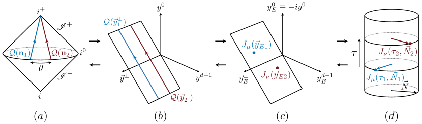
Figure 2: Diagram outlining our procedure for computing flux correlators, for the example of $\langle\mathcal{Q}\mathcal{Q}\rangle$. The flux operator $\mathcal{Q}(\mathbf{n})$ is defined as an integral of the $U(1)$ current over time for a fixed point on the celestial sphere $(a)$. To simplify the computation, the celestial sphere can be mapped to the null plane $y^{+}=0$ $(b)$. The Lorentzian correlator of the current $J_{\mu}(y)$ can then be computed by Wick rotating to the Euclidean plane $(c)$ and mapping to the Euclidean cylinder $(d)$, where the semiclassical approach of [11, 12] can be used. The result can then be mapped back to the original flux correlator via the same steps in reverse.

In short, our calculational procedure is:

1. Compute the Euclidean correlators

   $$\langle Q|\mspace{1.0mu}J_{\mu_{1}}(\tau_{1},\vec{N}_{1})\mspace{1.0mu}\cdots\mspace{1.0mu}J_{\mu_{k}}(\tau_{k},\vec{N}_{k})\mspace{1.0mu}|Q\rangle,\quad\langle Q|\mspace{1.0mu}T_{\mu_{1}\nu_{1}}(\tau_{1},\vec{N}_{1})\mspace{1.0mu}\cdots\mspace{1.0mu}T_{\mu_{k}\nu_{k}}(\tau_{k},\vec{N}_{k})\mspace{1.0mu}|Q\rangle,$$

   on the cylinder using the effective action arising from the finite charge density background, where $|Q\rangle$ is the ground state in radial quantization with fixed charge $Q$.

2. Map from the cylinder to the plane to obtain the Euclidean correlators

   $$\langle\overline{\mathcal{O}}_{Q}(\vec{y}_{Ef})\mspace{1.0mu}J_{\mu_{1}}(\vec{y}_{E1})\mspace{1.0mu}\cdots\mspace{1.0mu}J_{\mu_{k}}(\vec{y}_{Ek})\mspace{1.0mu}\mathcal{O}_{Q}(\vec{y}_{Ei})\rangle,\quad\langle\overline{\mathcal{O}}_{Q}(\vec{y}_{Ef})\mspace{1.0mu}T_{\mu_{1}\nu_{1}}(\vec{y}_{E1})\mspace{1.0mu}\cdots\mspace{1.0mu}T_{\mu_{k}\nu_{k}}(\vec{y}_{Ek})\mspace{1.0mu}\mathcal{O}_{Q}(\vec{y}_{Ei})\rangle.$$

3. Wick rotate to Lorentzian signature and integrate over $y_{1}^{-},\,\ldots,\,y_{k}^{-}$ to obtain the light-ray correlators

   $$\langle\overline{\mathcal{O}}_{Q}(y_{f})\mspace{1.0mu}\mathcal{Q}(\vec{y}^{\perp}_{1})\mspace{1.0mu}\cdots\mspace{1.0mu}\mathcal{Q}(\vec{y}^{\perp}_{k})\mspace{1.0mu}\mathcal{O}_{Q}(y_{i})\rangle,\quad\langle\overline{\mathcal{O}}_{Q}(y_{f})\mspace{1.0mu}\mathcal{E}(\vec{y}^{\perp}_{1})\mspace{1.0mu}\cdots\mspace{1.0mu}\mathcal{E}(\vec{y}^{\perp}_{k})\mspace{1.0mu}\mathcal{O}_{Q}(y_{i})\rangle.$$

4. Map to the celestial sphere and Fourier transform the positions of the external operators to momentum space to obtain the final correlation functions

   $$\langle\mathcal{Q}(\mathbf{n}_{1})\mspace{1.0mu}\cdots\mspace{1.0mu}\mathcal{Q}(\mathbf{n}_{k})\rangle,\quad\langle\mathcal{E}(\mathbf{n}_{1})\mspace{1.0mu}\cdots\mspace{1.0mu}\mathcal{E}(\mathbf{n}_{k})\rangle.$$

3 Warmup: Free Scalar

Before computing correlators with the semiclassical expansion, it is instructive to first consider the case of a free complex scalar field $\phi$, in order to gain some intuition for the structure of flux correlators and clarify some technical details of our procedure. Here we will focus on the two-point charge flux correlator in the background of the operator $\phi^{n}$ with $U(1)$ charge $Q=n$,

$$\langle\mathcal{Q}(\mathbf{n}_{1})\mspace{1.0mu}\mathcal{Q}(\mathbf{n}_{2})\rangle\equiv\frac{\langle\bar{\phi}^{n}(E)\mspace{1.0mu}\mathcal{Q}(\mathbf{n}_{1})\mspace{1.0mu}\mathcal{Q}(\mathbf{n}_{2})\mspace{1.0mu}\phi^{n}(E)\rangle}{\langle\bar{\phi}^{n}(E)\mspace{1.0mu}\phi^{n}(E)\rangle},$$ (3.1)

as well as the energy flux two-point function $\langle\mathcal{E}(\mathbf{n}_{1})\mathcal{E}(\mathbf{n}_{2})\rangle$.

As discussed in [29], the one-point flux correlators in the background of any scalar external source are completely fixed by rotational invariance and the requirement that the integral over all possible directions $\mathbf{n}$ gives the total charge or energy, respectively, leading to the expressions:

$$\langle\mathcal{Q}(\mathbf{n})\rangle=\frac{n}{\Omega_{d-2}},\quad\langle\mathcal{E}(\mathbf{n})\rangle=\frac{E}{\Omega_{d-2}}.$$ (3.2)

On the other hand, the two-point correlator can have non-trivial dependence on the angle $\mathbf{n}_{1}\cdot\mathbf{n}_{2}=\cos\theta$ between the two operators on the celestial sphere. In the case of free field theory, the correlation function can be computed diagrammatically in terms of the Wightman functions, which read

$$\langle\bar{\phi}(y_{1})\mspace{1.0mu}\phi(y_{2})\rangle=\frac{(-1)^{\frac{2-d}{2}}}{(d-2)\Omega_{d-1}\big{(}(y_{12}^{+}-i\epsilon_{12})(y_{12}^{-}-i\epsilon_{12})-|\vec{y}_{12}^{\perp}|^{2}\big{)}^{\frac{d-2}{2}}},$$ (3.3)

where $y_{12}^{\mu}\equiv y_{1}^{\mu}-y_{2}^{\mu}$ and the infinitesimal $\epsilon_{12}>0$ ensures proper Wightman ordering, i.e. $\phi(y_{2})$ acts before $\bar{\phi}(y_{1})$ (see, e.g., [48]).

For a free complex scalar field, the $U(1)$ current is given by

$$J_{\mu}=i\big{(}\phi(\partial_{\mu}\bar{\phi})-(\partial_{\mu}\phi)\bar{\phi}\big{)},$$ (3.4)

which is normalized such that the field $\phi$ has unit charge. To compute the charge flux correlator (3.1), we first need the four-point function $\langle\bar{\phi}^{n}J_{-}J_{-}\phi^{n}\rangle$. The resulting expression, normalized by the two-point function of $\phi^{n}$, is

$$\frac{\langle\bar{\phi}^{n}(y_{f})\mspace{1.0mu}J_{-}(y_{1})\mspace{1.0mu}J_{-}(y_{2})\mspace{1.0mu}\phi^{n}(y_{i})\rangle}{\langle\bar{\phi}^{n}(y_{f})\mspace{1.0mu}\phi^{n}(y_{i})\rangle}$$ (3.5)

$$\quad=(-1)^{d-1}\frac{n(n-1)}{(2\Omega_{d-1})^{2}}\frac{y_{fi}^{2(d-2)}}{y_{f1}^{d-2}y_{1i}^{d-2}y_{f2}^{d-2}y_{2i}^{d-2}}\bigg{(}\frac{y_{f1}^{+}}{y_{f1}^{2}}+\frac{y_{1i}^{+}}{y_{1i}^{2}}\bigg{)}\bigg{(}\frac{y_{f2}^{+}}{y_{f2}^{2}}+\frac{y_{2i}^{+}}{y_{2i}^{2}}\bigg{)}$$

$$\quad\quad+(-1)^{d-1}\frac{n}{(2\Omega_{d-1})^{2}}\frac{y_{fi}^{d-2}}{y_{f1}^{d-2}y_{12}^{d-2}y_{2i}^{d-2}}\Bigg{(}\bigg{(}\frac{y_{f1}^{+}}{y_{f1}^{2}}+\frac{y_{12}^{+}}{y_{12}^{2}}\bigg{)}\bigg{(}\frac{y_{12}^{+}}{y_{12}^{2}}+\frac{y_{2i}^{+}}{y_{2i}^{2}}\bigg{)}+\bigg{(}\frac{2}{d-2}\bigg{)}\frac{(y_{12}^{+})^{2}}{y_{12}^{4}}\Bigg{)}$$

$$\quad\quad+\,\ldots,$$

where the “$...$” stand for contributions to the four-point function that vanish upon integration over $y_{1}^{-}$ or $y_{2}^{-}$ and therefore do not contribute to the resulting flux correlator, leaving only the two Wick contractions shown in Figure 3. To simplify this expression, we have introduced the shorthand

$$y_{jk}^{2}\equiv(y_{jk}^{+}-i\epsilon_{jk})(y_{jk}^{-}-i\epsilon_{jk})-|\vec{y}_{jk}^{\perp}|^{2},$$ (3.6)

with $\epsilon_{f}>\epsilon_{1}>\epsilon_{2}>\epsilon_{i}$.

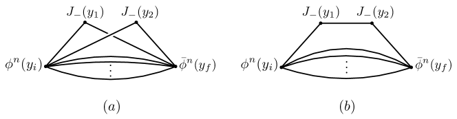
Figure 3: The two types of Wick contractions which contribute to the correlator $\langle\bar{\phi}^{n}\mathcal{Q}\mathcal{Q}\phi^{n}\rangle$ in free theory. The potential contributions from all other Wick contractions vanish upon integrating $y_{1}^{-}$ and $y_{2}^{-}$. The vertical dots indicate the propagators of the $n-2$ “spectator” particles for diagram $(a)$ and the $n-1$ spectators for diagram $(b)$.

We then need to integrate over $y_{1}^{-}$ and $y_{2}^{-}$ to obtain a correlator of charge light-ray operators. Finally, we can use the conformal transformation in eq. (2.2) to map to $x$-coordinates and obtain the charge flux correlator,

$$\frac{\langle\bar{\phi}^{n}(x_{f})\mspace{1.0mu}\mathcal{Q}(\mathbf{n}_{1})\mspace{1.0mu}\mathcal{Q}(\mathbf{n}_{2})\mspace{1.0mu}\phi^{n}(x_{i})\rangle}{\langle\bar{\phi}^{n}(x_{f})\mspace{1.0mu}\phi^{n}(x_{i})\rangle}$$ (3.7)

$$\qquad\qquad=\frac{n(n-1)}{\Omega_{d-2}^{2}}\frac{x_{fi}^{2(d-2)}}{(n_{1}\cdot x_{fi})^{d-2}\mspace{1.0mu}(n_{2}\cdot x_{fi})^{d-2}}+\frac{n}{\Omega_{d-2}}\frac{x_{fi}^{d-2}}{(n_{1}\cdot x_{fi})^{d-2}}\,\delta(\mathbf{n}_{1}-\mathbf{n}_{2}),$$

where we have introduced the null vectors $n_{j}^{\mu}\equiv(1,\mathbf{n}_{j})$, and the delta function is defined such that $\int d\Omega_{d-2}\,\delta(\mathbf{n}-\mathbf{n}^{\prime})=1$, for any unit vector $\mathbf{n}^{\prime}$. The details of this calculation are shown in Appendix B.

This expression only depends on the separation $x_{fi}$ between the two external sources. Indeed $\mathcal{Q}(\mathbf{n})$ is a translation invariant operator. Translation invariance of the full correlator implies that it only depends on $x_{fi}$. The two-point function (3.1)’s source has definite energy $E$, and is thus obtained by performing a Fourier transform of $x_{fi}$. After normalizing by the two-point function of $\phi^{n}$ (see Appendix B for details), we obtain:

$$\langle\mathcal{Q}(\mathbf{n}_{1})\mspace{1.0mu}\mathcal{Q}(\mathbf{n}_{2})\rangle$$ (3.8)

$$\quad=\frac{n(n-1)}{\Omega_{d-2}^{2}}\frac{\Gamma\big{(}(n-1)(\tfrac{d-2}{2})\big{)}\Gamma\big{(}n(\tfrac{d-2}{2})\big{)}}{\Gamma\big{(}(n-2)(\tfrac{d-2}{2})\big{)}\Gamma\big{(}(n+1)(\tfrac{d-2}{2})\big{)}}\,{}_{2}F_{1}\Big{(}d-2,d-2;(n+1)(\tfrac{d-2}{2});\sin^{2}\!\tfrac{\theta}{2}\Big{)}$$

$$\quad\quad+\,\frac{n}{\Omega_{d-2}}\delta(\mathbf{n}_{1}-\mathbf{n}_{2}).$$

For finite $n$, this correlator has non-trivial dependence on the angle $\theta$ between the two directions on the celestial sphere, as shown in Figure 4. This dependence is easily understood from momentum conservation: for a source at rest, measuring charge flux in one direction increases the likelihood of measuring flux in the opposite direction. This effect is particularly visible for $n=2$, where eq. (3.8) reduces to a sum of delta functions at $\theta=0$ and $\theta=\pi$. At large $n$, however, this expression converges to the homogeneous distribution

$$\langle\mathcal{Q}(\mathbf{n}_{1})\mspace{1.0mu}\mathcal{Q}(\mathbf{n}_{2})\rangle\approx\bigg{(}\frac{n}{\Omega_{d-2}}\bigg{)}^{2}\left(1+\frac{\Omega_{d-2}}{n}\left[\delta(\mathbf{n}_{1}-\mathbf{n}_{2})-\frac{1+(d-2)\cos\theta}{\Omega_{d-2}}\right]+O(n^{-2})\right).$$ (3.9)

The fact that the very non-trivial expression (3.8) simplifies immensely at leading order in $n$ is understood by noticing that the result can also be found as a saddle point expansion at large $n$ in the path integral. We therefore already see in free theory a first hint that the correct framework to study the large charge regime is a semiclassical expansion.

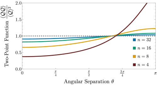
Figure 4: Charge flux two-point correlator $\langle\mathcal{Q}\mathcal{Q}\rangle$ as a function of the angle $\theta$ between the two flux operators in the background of $\phi^{4}$ (red), $\phi^{8}$ (gold), $\phi^{16}$ (green), and $\phi^{32}$ (blue), normalized by the homogeneous solution $\langle\mathcal{Q}\rangle^{2}$. The delta function at $\theta=0$ is not shown.

We can repeat this same calculation for the energy flux operator, with the same diagrammatic contributions as Figure 3. The final result is:

$$\langle\mathcal{E}(\mathbf{n}_{1})\mspace{1.0mu}\mathcal{E}(\mathbf{n}_{2})\rangle$$ (3.10)

$$\quad=\frac{E^{2}}{\Omega_{d-2}^{2}}\frac{\Gamma\big{(}(n-1)(\tfrac{d-2}{2})+1\big{)}\Gamma\big{(}n(\tfrac{d-2}{2})+1\big{)}}{\Gamma\big{(}(n-2)(\tfrac{d-2}{2})\big{)}\Gamma\big{(}(n+1)(\tfrac{d-2}{2})+2\big{)}}\,{}_{2}F_{1}\Big{(}d-1,d-1;(n+1)(\tfrac{d-2}{2})+2;\sin^{2}\!\tfrac{\theta}{2}\Big{)}$$

$$\quad\quad+\,\frac{E^{2}}{\Omega_{d-2}}\frac{d-1}{n(d-2)+2}\,\delta(\mathbf{n}_{1}-\mathbf{n}_{2}).$$

The behavior of this expression is analogous to that of the charge flux correlator, converging to the homogeneous distribution $\langle\mathcal{E}\rangle^{2}$ in the large $n$ limit

$$\langle\mathcal{E}(\mathbf{n}_{1})\mspace{1.0mu}\mathcal{E}(\mathbf{n}_{2})\rangle=\bigg{(}\frac{E}{\Omega_{d-2}}\bigg{)}^{2}\left(1+\frac{d-1}{d-2}\frac{\Omega_{d-2}}{n}\left[\delta(\mathbf{n}_{1}-\mathbf{n}_{2})-\frac{1+(d-1)\cos\theta}{\Omega_{d-2}}\right]+O(n^{-2})\right).$$ (3.11)

4 Flux Correlators at Large Charge

In this section, we compute the charge (and energy) flux correlators (1.4) in a semiclassical expansion at large charge. For this, we consider CFTs in $d>2$ spacetime dimensions with a $U(1)$ global symmetry and we follow the procedure presented in Section 2 to compute the correlators in the background of the lowest-dimension operator $\mathcal{O}_{Q}$ with $U(1)$ charge $Q$. We present the two possible contexts in which we can do the computation. The first possibility is to consider general CFTs with U(1) symmetry and to compute the correlators in the EFT of the Goldstone associated to the U(1) symmetry breaking [11, 12]. After briefly reviewing this approach, we apply it to the calculation of the two-point functions $\langle\mathcal{Q}\mathcal{Q}\rangle$ and $\langle\mathcal{E}\mathcal{E}\rangle$, before generalizing to the case with an arbitrary number of flux operator insertions. While this method has the advantage of being valid for a large class of CFTs, it only investigates the many quanta regime (which in the context of the EFT can be rephrased as the large chemical potential limit $\mu\gg 1$). We therefore proceed by showing the computation for a UV-complete theory, the Wilson-Fisher fixed point in $4-\epsilon$ dimensions, where we lose the universality of the result but the semiclassical expansion becomes valid for all values of $\lambda_{*}n$ (or $\mu$). Finally, we motivate the validity of the EFT to compute the charge and energy flux correlators in Minkowski space.

4.1 Review of Semiclassics at Large Charge

Consider a general Euclidean CFT correlation function of the form

$$\langle\overline{\mathcal{O}}_{Q}(\vec{y}_{Ef})\mspace{1.0mu}\mathcal{O}_{1}(\vec{y}_{E1})\mspace{1.0mu}\cdots\mspace{1.0mu}\mathcal{O}_{k}(\vec{y}_{Ek})\mspace{1.0mu}\mathcal{O}_{Q}(\vec{y}_{Ei})\rangle,$$ (4.1)

where the intermediate operators $\mathcal{O}_{j}$ have fixed $U(1)$ charges $q_{j}\ll Q$ and scaling dimensions $\Delta_{j}\ll\Delta_{Q}$ (such as the conserved current $J_{\mu}$ or stress tensor $T_{\mu\nu}$). Applying conformal transformations, we can always set $y_{i}\to 0$ and $y_{f}\to\infty$. Then, by Weyl mapping to the Euclidean cylinder, we relate eq. (4.1), up to a known rescaling factor, to the cylinder correlator

$$\langle Q|\mspace{1.0mu}\mathcal{O}_{1}(\tau_{1},\vec{N}_{1})\mspace{1.0mu}\cdots\mspace{1.0mu}\mathcal{O}_{k}(\tau_{k},\vec{N}_{k})\mspace{1.0mu}|Q\rangle,$$ (4.2)

where

$$|Q\rangle\equiv\lim_{\tau\to-\infty}e^{-\Delta_{Q}\tau}\mathcal{O}_{Q}(\tau,\vec{N})|0\rangle\,,\qquad\langle Q|\equiv\lim_{\tau\to\infty}e^{\Delta_{Q}\tau}\langle 0|\mathcal{O}_{Q}(\tau,\vec{N}),$$

is the ground state in radial quantization of the conformal multiplet generated by $\mathcal{O}_{Q}$. The insight of [11, 12] is that, for large $Q$: (i) eq. (4.2) can be computed by a systematic expansion around a saddle point in the path integral; (ii) the dynamics around the saddle configuration can be largely determined by symmetry considerations. The simplest option as concerns the second point is that the saddle configuration realizes the spontaneous symmetry breaking

$$SO(d+1,1)\times U(1)\to SO(d)\times D^{\prime},$$ (4.3)

where $D^{\prime}$ is the unbroken combination

$$D^{\prime}\equiv D+\mu Q,$$ (4.4)

of dilatations $D$ and of the $U(1)$ charge $Q$, which implements the time translation invariance of the saddle solution. Such a symmetry breaking pattern characterizes the configuration as a conformal superfluid. The parameter $\mu$ has then the standard interpretation of a chemical potential (see for instance [49]). Eq. (4.3) dictates the presence of (just) one soft Goldstone mode whose properties are largely fixed by symmetry. This is the analogue (with the addition of conformal symmetry) of the hydrodynamic sound mode of ordinary superfluids. The simplest and most natural option is that this is the only soft mode, while all other modes, which have no symmetry reason to be light, are gapped at the only available mass scale in the system, $\mu$. In several several specific calculable models, this natural set of assumptions has been explicitly verified [16, 17, 19, 18].

Under the above hypotheses, the computation of the correlators reduces to a path integral controlled by the effective action for the Goldstone mode. The inserted operators are matched to local functions of the Goldstone field and its derivatives, precisely like in QCD when mapping quark-gluon operators to mesonic ones. At leading order in the derivative expansion, the effective Lagrangian is given by

$$\mathcal{L}_{\textrm{eff}}[\chi]\approx-c_{1}(-\partial^{\mu}\chi\partial_{\mu}\chi)^{\frac{d}{2}}+\ldots,$$ (4.5)

with $c_{1}$ is a theory-dependent Wilson coefficient. Setting the cylinder radius to $R=1$, the boundary condition corresponding to the state $|Q\rangle$ is implemented by adding the term $i\dot{\chi}Q/\Omega_{d-1}$ to the Lagrangian [12] in the path integral. The resulting equations of motion

$$J^{0}\equiv\frac{\partial\mathcal{L}_{\textrm{eff}}}{\partial\dot{\chi}}=i\frac{Q}{\Omega_{d-1}},$$

have the spatially homogeneous solution

$$\chi(\tau,\vec{N})=-i\mu\tau+\textrm{constant},$$ (4.6)

with the chemical potential $\mu$ satisfying

$$c_{1}\mu^{d-1}\approx\frac{Q}{\Omega_{d-1}}\,\quad\Rightarrow\quad\mu\sim Q^{\frac{1}{d-1}}.$$ (4.7)

Replacing the solution back into the action finally gives the relation between scaling dimension and charge

$$\Delta_{Q}^{d-1}=\frac{(d-1)^{d-1}}{\Omega_{d-1}d^{d}}\frac{Q^{d}}{c_{1}}\Big{(}1+O(1/Q^{\frac{2}{d-1}})\Big{)}\,.$$ (4.8)

We can now use the classical solution to compute the leading behavior of correlation functions at large $Q$. To do so, we match the conserved currents in the correlation functions to the corresponding objects built out of eq. (4.5). For example, the $U(1)$ current is given by

$$J_{\mu}=c_{1}d(-\partial^{\alpha}\chi\partial_{\alpha}\chi)^{\frac{d-2}{2}}\partial_{\mu}\chi,$$ (4.9)

while the stress tensor is

$$T_{\mu\nu}=c_{1}d(-\partial^{\alpha}\chi\partial_{\alpha}\chi)^{\frac{d-2}{2}}\partial_{\mu}\chi\partial_{\nu}\chi+c_{1}(-\partial^{\alpha}\chi\partial_{\alpha}\chi)^{\frac{d}{2}}g_{\mu\nu}.$$ (4.10)

Using eq. (4.6) in the above expressions, at leading order in the large $Q$ expansion we then have

$$\langle J_{\mu}\rangle \equiv\frac{\langle Q|\mspace{1.0mu}J_{\mu}(\tau,\vec{N})\mspace{1.0mu}|Q\rangle}{\langle Q|Q\rangle}=-ic_{1}d\mu^{d-1}\delta^{\tau}_{\,\mu}=-\frac{iQ}{\Omega_{d-1}}\delta^{\tau}_{\,\mu},$$ (4.11)

$$\langle T_{\mu\nu}\rangle \equiv\frac{\langle Q|\mspace{1.0mu}T_{\mu\nu}(\tau,\vec{N})\mspace{1.0mu}|Q\rangle}{\langle Q|Q\rangle}=-c_{1}d\mu^{d}\Big{(}\delta^{\tau}_{\,\mu}\delta^{\tau}_{\,\nu}-\frac{1}{d}g_{\mu\nu}\Big{)}=-\frac{d}{d-1}\frac{\Delta_{Q}}{\Omega_{d-1}}\Big{(}\delta^{\tau}_{\,\mu}\delta^{\tau}_{\,\nu}-\frac{1}{d}g_{\mu\nu}\Big{)}.$$

4.2 Application to Flux Two-Point Function

Our goal is to now adapt the semiclassical approach to the calculation of the flux operator correlation functions (3.1). Following the procedure laid out in sec. 2, we first need to compute the associated correlator on the Euclidean cylinder using the semiclassical solution (4.6). For the current two-point function, we obtain the simple expression,

$$\frac{\langle Q|\mspace{1.0mu}J_{\mu}(\tau_{1},\vec{N}_{1})\mspace{1.0mu}J_{\nu}(\tau_{2},\vec{N}_{2})\mspace{1.0mu}|Q\rangle}{\langle Q|Q\rangle}=\langle J_{\mu}\rangle\langle J_{\nu}\rangle=-\bigg{(}\frac{Q}{\Omega_{d-1}}\bigg{)}^{2}\delta^{\tau}_{\,\mu}\delta^{\tau}_{\,\nu}.$$ (4.12)

Next, we need to map this correlation function from the cylinder to the Euclidean plane, with all four operators at arbitrary positions. The most general way to do so is to decompose this four-point function into the set of independent tensor structures allowed by conformal symmetry, whose behavior under conformal transformations is known.

Fortunately, because this leading contribution factorizes into a product of CFT two- and three-point functions, which are completely fixed by conformal invariance, we can directly map the individual terms to the Euclidean plane, then Wick rotate to obtain the resulting Lorentzian correlator in $y$-coordinates. Focusing on the only relevant component $J_{-}$, one then finds

$$\frac{\langle\overline{\mathcal{O}}_{Q}(y_{f})\mspace{1.0mu}J_{-}(y_{1})\mspace{1.0mu}J_{-}(y_{2})\mspace{1.0mu}\mathcal{O}_{Q}(y_{i})\rangle}{\langle\overline{\mathcal{O}}_{Q}(y_{f})\mspace{1.0mu}\mathcal{O}_{Q}(y_{i})\rangle}=\frac{\langle\overline{\mathcal{O}}_{Q}(y_{f})\mspace{1.0mu}J_{-}(y_{1})\mspace{1.0mu}\mathcal{O}_{Q}(y_{i})\rangle\mspace{1.0mu}\langle\overline{\mathcal{O}}_{Q}(y_{f})\mspace{1.0mu}J_{-}(y_{2})\mspace{1.0mu}\mathcal{O}_{Q}(y_{i})\rangle}{\langle\overline{\mathcal{O}}_{Q}(y_{f})\mspace{1.0mu}\mathcal{O}_{Q}(y_{i})\rangle^{2}}$$ (4.13)

$$\qquad\qquad=(-1)^{d-1}\bigg{(}\frac{Q}{2\Omega_{d-1}}\bigg{)}^{2}\frac{y_{fi}^{2(d-2)}}{y_{f1}^{d-2}y_{1i}^{d-2}y_{f2}^{d-2}y_{2i}^{d-2}}\bigg{(}\frac{y_{f1}^{+}}{y_{f1}^{2}}+\frac{y_{1i}^{+}}{y_{1i}^{2}}\bigg{)}\bigg{(}\frac{y_{f2}^{+}}{y_{f2}^{2}}+\frac{y_{2i}^{+}}{y_{2i}^{2}}\bigg{)}.$$

The more general analysis in terms of four-point function tensor structures, which is needed for computing subleading corrections in $1/Q$, is shown in appendix B.

The position-dependence of the four-point function (4.13) is identical to the first term in the free theory result from eq. (3.5). We can therefore repeat the same analysis to obtain the resulting charge flux two-point function in $x$-coordinates,

$$\frac{\langle\overline{\mathcal{O}}_{Q}(x_{f})\mspace{1.0mu}\mathcal{Q}(\mathbf{n}_{1})\mspace{1.0mu}\mathcal{Q}(\mathbf{n}_{2})\mspace{1.0mu}\mathcal{O}_{Q}(x_{i})\rangle}{\langle\overline{\mathcal{O}}_{Q}(x_{f})\mspace{1.0mu}\mathcal{O}_{Q}(x_{i})\rangle}=\bigg{(}\frac{Q}{\Omega_{d-2}}\bigg{)}^{2}\frac{x_{fi}^{2(d-2)}}{(n_{1}\cdot x_{fi})^{d-2}\,(n_{2}\cdot x_{fi})^{d-2}}.$$ (4.14)

The charge flux two-point function for a source with definite momentum is then found the same way as for the free scalar field, though in this case, we can only keep the leading behavior of the Fourier transform at large $Q$, as subleading terms get contributions from higher orders in the EFT expansion as well as non-perturbative effects. We therefore obtain the resulting leading order behavior

$$\langle\mathcal{Q}(\mathbf{n}_{1})\mspace{1.0mu}\mathcal{Q}(\mathbf{n}_{2})\rangle\approx\bigg{(}\frac{Q}{\Omega_{d-2}}\bigg{)}^{2}\Big{(}1+O(1/\Delta_{Q})\Big{)}\qquad(Q\to\infty).$$ (4.15)

We can repeat this same procedure for the energy flux two-point function, obtaining

$$\langle\mathcal{E}(\mathbf{n}_{1})\mspace{1.0mu}\mathcal{E}(\mathbf{n}_{2})\rangle\approx\bigg{(}\frac{E}{\Omega_{d-2}}\bigg{)}^{2}\Big{(}1+O(1/\Delta_{Q})\Big{)}\qquad(Q\to\infty).$$ (4.16)

We thus found that in any $U(1)$ symmetric CFT satisfying the broad hypotheses of the large charge expansion, the lowest-dimension operator $\mathcal{O}_{Q}$ with charge $Q$ creates a state of homogeneous charge and energy density as $Q\to\infty$, with any inhomogeneities suppressed by $1/\Delta_{Q}$.

4.3 Generalization to Higher-Point Functions

This analysis can be extended to correlation functions involving an arbitrary number of flux operator insertions, so long as the number of operators $k$ is sufficiently small compared to the total charge $Q$. Starting with the $k$-point function on the cylinder, the leading semiclassical result is simply a product of $k$ expectation values,

$$\frac{\langle Q|\mspace{1.0mu}J_{\mu_{1}}(\tau_{1},\vec{N}_{1})\mspace{1.0mu}\cdots\mspace{1.0mu}J_{\mu_{k}}(\tau_{k},\vec{N}_{k})\mspace{1.0mu}|Q\rangle}{\langle Q|Q\rangle}=\langle J_{\mu_{1}}\rangle\cdots\langle J_{\mu_{k}}\rangle,$$ (4.17)

with an analogous expression for $k$ insertions of the stress tensor.

Because this $k$-point function factorizes into a product of two- and three-point functions, we can again easily map to the Euclidean plane, Wick rotate, and integrate to obtain a similarly factorized Lorentzian correlator in $x$-coordinates:

$$\frac{\langle\overline{\mathcal{O}}_{Q}(x_{f})\mspace{1.0mu}\mathcal{Q}(\mathbf{n}_{1})\mspace{1.0mu}\cdots\mspace{1.0mu}\mathcal{Q}(\mathbf{n}_{k})\mspace{1.0mu}\mathcal{O}_{Q}(x_{i})\rangle}{\langle\overline{\mathcal{O}}_{Q}(x_{f})\mspace{1.0mu}\mathcal{O}_{Q}(x_{i})\rangle}=\bigg{(}\frac{Q}{\Omega_{d-2}}\bigg{)}^{k}\frac{x_{fi}^{k(d-2)}}{(n_{1}\cdot x_{fi})^{d-2}\cdots(n_{k}\cdot x_{fi})^{d-2}}.$$ (4.18)

While the Fourier transform of this general correlator to momentum space is unknown, we can still determine its leading behavior at large $Q$, as explained in detail in appendix B. The result is

$$\langle\mathcal{Q}(\mathbf{n}_{1})\mspace{1.0mu}\cdots\mspace{1.0mu}\mathcal{Q}(\mathbf{n}_{k})\rangle\approx\bigg{(}\frac{Q}{\Omega_{d-2}}\bigg{)}^{k}\Big{(}1+O(k^{2}/Q^{\frac{d}{d-1}})\Big{)}\qquad(Q\to\infty),$$ (4.19)

with a similar expression for the energy flux $k$-point function,

$$\langle\mathcal{E}(\mathbf{n}_{1})\mspace{1.0mu}\cdots\mspace{1.0mu}\mathcal{E}(\mathbf{n}_{k})\rangle\approx\bigg{(}\frac{E}{\Omega_{d-2}}\bigg{)}^{k}\Big{(}1+O(k^{2}/Q^{\frac{d}{d-1}})\Big{)}\qquad(Q\to\infty).$$ (4.20)

So long as $k\ll\sqrt{\Delta_{Q}}$, we therefore expect all flux correlation functions to be homogeneous in the background of the large charge operator $\mathcal{O}_{Q}$.

4.4 Large Charge at the Wilson-Fisher Fixed Point

The EFT calculation presented above describes the universal large charge regime for a broad class of CFTs that meet the generic hypotheses outlined in Section 4.1. As demonstrated in [17], this EFT can be effectively applied to the Wilson-Fisher fixed points in the asymptotic regime $\lambda_{*}n\gg 1$. On the other hand, Wilson-Fisher models admit a semiclassical description for arbitrary values of $\lambda_{*}n$ (as long as $n\gg 1$), offering a well-defined framework to thoroughly explore the transition from the few ($\lambda_{*}n\ll 1$) to the many ($\lambda_{*}n\gg 1$) quanta regime. This subsection is devoted to the simplest Wilson-Fisher model consisting of a complex scalar field $\phi$ with quartic coupling $\frac{\lambda}{4}(\bar{\phi}\phi)^{2}$ at its fixed point in $d=4-\epsilon$ [17]. The UV completeness of the Wilson-Fisher model also allows us to bypass the issue of the potential breakdown of the EFT description, which we discuss in Section 4.5.

Working directly on the cylinder (we again take $R=1$), the action for the $O(2)$ Wilson-Fisher model reads:

$$S=\int d^{d}x\sqrt{g}\left[g^{\mu\nu}\partial_{\mu}\bar{\phi}\partial_{\nu}\phi+\bigg{(}\frac{d-2}{2}\bigg{)}^{2}\mspace{1.0mu}\bar{\phi}\phi+\frac{\lambda_{*}}{4}\mspace{1.0mu}(\bar{\phi}\phi)^{2}\right],$$ (4.21)

where the mass term is dictated by conformal invariance and controlled by the spatial curvature of the cylinder. It is convenient to reexpress the complex field as

$$\phi=\frac{\rho}{\sqrt{2}}e^{i\chi}.$$ (4.22)

In the charge $n$ ground state created by $\phi^{n}$, the spatially homogeneous solution of the equations of motion takes the form

$$\rho=f=\textnormal{constant},\qquad\chi=-i\mu\tau+\textnormal{constant},$$ (4.23)

with the parameters satisfying the constraints

$$\mu^{2}-\left(\frac{d-2}{2}\right)^{2}=\frac{\lambda_{*}}{4}f^{2},\qquad\mu f^{2}\Omega_{d-1}=n.$$ (4.24)

The first constraint corresponds to the equations of motion, while the second fixes the total charge to $n$.

Expanding the action at quadratic order in the two independent fluctuations $\sigma(x)$ and $\pi(x)$

$$\rho(x)=f+\sigma(x),\qquad\chi(x)=-i\mu\tau+\frac{\pi(x)}{\sqrt{2}f},$$ (4.25)

we obtain the spectrum

$$\omega^{2}_{\pm}(\ell)=J_{\ell}^{2}+3\mu^{2}-\big{(}\tfrac{d-2}{2}\big{)}^{2}\pm\sqrt{\Big{(}3\mu^{2}-\big{(}\tfrac{d-2}{2}\big{)}^{2}\Big{)}^{2}+4J_{\ell}^{2}\mu^{2}},$$ (4.26)

with $J_{\ell}^{2}\equiv\ell(\ell+d-2)$. Taking the large $\mu$ limit (or equivalently $\lambda n\gg 1$), the $\omega_{+}(\ell)$ modes decouple as they exhibit a gap $\mu$, while the $\omega_{-}(\ell)$ modes reduce to the spectrum of the Goldstone mode of the EFT. The EFT Lagrangian (4.5) is recovered by integrating out the radial mode $r(x)$.

Like in the EFT, the operators are local functions of the fields. The $U(1)$ current is

$$J_{\mu}=i\rho^{2}\partial_{\mu}\chi,$$ (4.27)

while the stress tensor is

$$\begin{split}T_{\mu\nu}=&\rho^{2}\partial_{\mu}\chi\partial_{\nu}\chi+\frac{2}{3}\partial_{\mu}\rho\partial_{\nu}\rho\ -\frac{1}{3}\rho\partial_{\mu}\partial_{\nu}\rho\\ -&g_{\mu\nu}\bigg{[}\frac{\rho^{2}}{2}(\partial\chi)^{2}+\frac{1}{2}(\partial\rho)^{2}-\frac{1}{6}\partial_{\sigma}\partial^{\sigma}\rho^{2}+\frac{1}{2}\bigg{(}\frac{d-2}{2}\bigg{)}^{2}\rho^{2}+\frac{\lambda_{*}}{16}\rho^{4}\bigg{]}.\end{split}$$ (4.28)

In the limit where the radial mode decouples, we recover eqs. (4.9) and (4.10).

The expectation values of $J_{\mu}$ and $T_{\mu\nu}$ in the background of $\phi^{n}$, when expressed in terms of the quantum numbers $n$ and $\Delta_{n}$, coincide with the EFT result in eq. (4.11) for any value of $\lambda_{*}n\simeq\epsilon n$, not only for $\lambda_{*}n\gg 1$. This is unsurprising as this result is dictated by Ward identities. At leading order in the semiclassical expansion, the higher-point current correlators therefore exactly match those of the EFT found in Section 4.2, as they are simply given by products of the expectation values. Repeating the same analysis as for the EFT, we therefore find

$$\hat{h}^{(0)}(\epsilon n,\theta)=0.$$ (4.29)

Crucially, this result holds for arbitrary $\epsilon n$ ($\simeq\lambda_{*}n$), as long as $n\gg 1$.

Besides offering an explicit realization of the generic EFT, the Wilson-Fisher theory enables us to study better the transition from few to many quanta. Contrary to what happens for the scaling dimension $\Delta_{Q}$ studied in [17], which exhibits qualitatively different behavior in the two regimes, we find that the leading correction to homogeneity $\hat{h}^{(0)}(\epsilon n,\theta)$ vanishes identically in both regimes.

4.5 Breakdown of Lorentzian EFT

In Section 4.2, we derived the Lorentzian correlators by first computing on the Euclidean cylinder at leading order in the EFT and then analytically continuing the result to the Lorentzian plane. However, the computation on the Euclidean cylinder is reliable only in the kinematical regime of validity of the EFT. With the charge $Q$ and $-Q$ operators inserted at respectively $\tau\to-\infty$ and $\tau\to+\infty$ (see section 4.1), the EFT regime corresponds to separations between individual insertions of the current or stress tensor that are larger than $1/\mu$. Equivalently, the EFT is defined by an expansion in powers of $\partial/\mu$. In particular, for the insertion of just two currents, as in eq. (4.12), the condition takes the form

$$|\tau_{1}-\tau_{2}|^{2}+\big{|}\arccos(\vec{N}_{1}\cdot\vec{N}_{2})\big{|}^{2}\gtrsim\frac{1}{\mu^{2}}.$$ (4.30)

Considering the corresponding correlator on the plane

$$\langle\bar{\cal O}_{Q}(x_{f})\mspace{1.0mu}J(x_{1})\mspace{1.0mu}J(x_{2})\mspace{1.0mu}{\cal O}_{Q}(x_{i})\rangle,$$

eq. (4.30) is phrased in terms of the conformal ratios

$$u\equiv\frac{x_{1i}^{2}\mspace{1.0mu}x_{2f}^{2}}{x_{1f}^{2}\mspace{1.0mu}x_{2i}^{2}}\,,\qquad v\equiv\frac{x_{12}^{2}\mspace{1.0mu}x_{if}^{2}}{x_{1f}^{2}\mspace{1.0mu}x_{2i}^{2}}\,,\qquad\Big{(}x_{ab}^{2}\equiv(x_{a}-x_{b})^{2}\Big{)},$$ (4.31)

as

$$\frac{\log^{2}(u)}{4}+\arccos^{2}\left(\frac{1+u-v}{2\sqrt{u}}\right)\gtrsim\frac{1}{\mu^{2}}\,.$$ (4.32)

For $\mu\gg 1$ the above condition can equivalently, and more simply, be expressed as

$$|1-u|\gtrsim\frac{1}{\mu}\quad\textnormal{and/or}\quad v\gtrsim\frac{1}{\mu^{2}}\,.$$ (4.33)

It is instructive to study these conditions for finite Euclidean $x_{i}$ and $x_{f}$, a choice similar to the one implied by the form of the state in eq. (1.3) when working in the Lorentzian plane. Using conformal transformations one can see that the coordinate choices satisfying eq. (4.33) can always essentially be mapped into a configuration where $x_{1}$ and $x_{2}$ are located in a compact region of size $\sim\mu x_{if}$ encircling $x_{i}$ and $x_{f}$, while remaining sufficiently separated, with roughly $x_{12}\gtrsim x_{if}/\mu$. This result is physically compatible with a picture where the insertion of ${\cal O}_{Q}(x_{i})$ and $\bar{\cal O}_{Q}(x_{f})$ creates a medium with a density of charge and energy, which is large in the surrounding region and decays at infinity. The power law nature of this decay is simply dictated by the 3-point function $\langle\bar{\cal O}_{Q}J{\cal O}_{Q}\rangle$. According to this picture, it is then physically intuitive that the semiclassical description works in the region of high density $x_{12}\lesssim x_{if}/\mu$, so long as $x_{12}$ is larger than the typical length $x_{if}/\mu$ associated with the medium density. Notice that, simply applying an inversion starting from the above configuration, we can always map one of the two observation points, say $x_{1}$, to $\infty$. As shown in Figure 5, the region of EFT validity then simply consists of the points where $x_{2}$ is in a ball of size $\mu x_{if}$ enclosing $x_{i}$ and $x_{f}$.

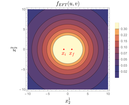
Figure 5: Value of the conformal invariant $f_{EFT}(u,v)\equiv\frac{\ln^{2}(u)}{4}+\arccos^{2}\left(\frac{1+u-v}{2\sqrt{u}}\right)$ as a function of the position of the insertion $x_{2}$ in the Euclidean plane. For simplicity, the function is plotted in two spatial dimensions $x_{2}\equiv(x_{2}^{1},x_{2}^{2})$. $x_{i}$ and $x_{f}$ are respectively chosen to be $(-1,0)$, $(1,0)$, represented on the plot as the two red points, and $x_{1}$ is sent to infinity. The EFT is valid for computing the four-point function as long as $f_{EFT}(u,v)\gtrsim\frac{1}{\mu^{2}}$. We observe that this is the case as long as $x_{2}$ is approximately inserted in a compact region of radius $\sim\mu|x_{if}|$, close to the “source” insertions $x_{i/f}$.

When considering the analytic continuation to Lorentzian signature, the range of $u$ and $v$ is extended to include all real values, not just positive ones. By analyticity, we expect the domain of validity of the EFT description to still be defined by eq. (4.33), with an added absolute value for $v$. Now, the flux correlators we have considered in this work are (partially) integrated quantities with respect to the coordinates defining $u$ and $v$. As we will now discuss, the integration region extends outside the domain defined by eq. (4.33), so that the flux correlators receive a contribution that cannot be systematically computed within the EFT, i.e. in terms of its Wilson coefficients. However, the region where eq. (4.33) is violated shrinks to a point in the limit $Q\to\infty$ (for which $\mu\to\infty$). Therefore, provided the correlators are not too singular in this region, we still expect this out-of-EFT contribution to vanish relative to the leading bulk contribution for $Q\to\infty$. It is under this assumption that the EFT computation done in the previous sections should be taken. While we think this assumption is justified, as indicated by the examples of UV complete models like Wilson-Fisher, we leave to future study a more detailed investigation of the effects due to this vanishing region of integration. In the remainder of this section, we will limit ourselves to discussing the spacetime description of the constraints in eq. (4.33) to offer an intuitive physical picture.

The relevant coordinate configuration is one where $x_{i}$ and $x_{f}$ are finite (with separation smaller than the length scale $\xi$ defined in (1.3)), while $x_{1}$ and $x_{2}$ are sent to infinity in a nearly lightlike direction. In light-cone radial coordinates this means $r_{1}^{+}\,,r_{2}^{+}\to\infty$ with $r_{1}^{-}\,,r_{2}^{-}$ fixed. In this limit, the conformal ratios take the form

$$u=\frac{(r_{1}^{-}-n_{1}\cdot x_{i})(r_{2}^{-}-n_{2}\cdot x_{f})}{(r_{1}^{-}-n_{1}\cdot x_{f})(r_{2}^{-}-n_{2}\cdot x_{i})}\,,\qquad v=\frac{x_{fi}^{2}\,n_{1}\cdot n_{2}}{2(r_{1}^{-}-n_{1}\cdot x_{f})(r_{2}^{-}-n_{2}\cdot x_{i})}\,,$$ (4.34)

where $n_{i}$ are the null vectors on the celestial sphere defined below eq. (3.7).

From (4.34), for $x_{i}\not=x_{f}$ and $n_{1}\not=n_{2}$ one finds that $u\to 1$ and $v\to 0$ as $|r_{1,2}^{-}|\to\infty$. However, the EFT requirement (4.33) is satisfied in a region of the $(r_{1}^{-},r_{2}^{-})$ plane that grows with $\mu$. In Figure 6, we show the shape of that region for spatially separated $x_{i}$ and $x_{f}$. One sees that the EFT region corresponds to a choice of $(r_{1}^{-},r_{2}^{-})$ such that at least one of the two observation points is near the light cone of the midpoint $(x_{i}+x_{f})/2$.

Like in the Euclidean case, this result has an intuitive physical interpretation. The insertion of the two charged operators essentially creates a shell of width controlled by $x_{fi}$ and centered around $(x_{i}+x_{f})/2$ that expands at the speed of light. One then expects the semiclassical description to apply well for $x_{1}$ and $x_{2}$ around the peak of this shell, where the charge density is large, and less so in the tails, where the density goes to zero and non-universal quantum fluctuations may become important. Notice that the EFT situation where both $x_{1}$ and $x_{2}$ are around the peak is conformally equivalent to one where only one is (similarly to what happens in the Euclidean case depicted in Figure 5). This explains the shape of the EFT regions in Figure 6.

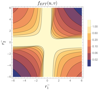
Figure 6: Value of the conformal invariant $f_{EFT}(u,v)\equiv\left|\frac{\ln(u)}{2}\right|^{2}+\left|\arccos\left(\frac{1+u-v}{2\sqrt{u}}\right)\right|^{2}$ as a function of $r_{1}^{-}$ and $r_{2}^{-}$ in the Lorentzian plane. $x_{i}=(0,0.5,0,0)$ and $x_{f}=(0,-0.5,0,0)$ are chosen to be space-like separated, though the result is qualitatively similar if the two points are time-like separated. We chose $n_{1}=(1,1,0,0)$ and $n_{2}=(1,0,1,0)$, hence the asymmetry between $r_{1}^{-}$ and $r_{2}^{-}$. Other choices for $n_{1,2}$ give qualitatively similar results, with the one shown here being the most asymmetric configuration. The EFT is valid for computing the four-point function as long as $f_{EFT}(u,v)\gtrsim\frac{1}{\mu^{2}}$.

The computation of flux correlators also requires integrating over the coordinates $x_{i}$ and $x_{f}$ to comply with the definition (1.3) of our chosen external state. We expect this integral to be dominated by the region $|x_{fi}|\sim 1/E$, $|x_{i}+x_{f}|\lesssim\xi$. The EFT will therefore apply for all configurations except those where both observation points $x_{1}$ and $x_{2}$ lie far outside of a thick light-cone-shaped region centered at $(x_{i}+x_{f})/2$ and whose thickness is controlled by $|x_{fi}|\sim 1/E$.

As we are dealing with a CFT where signals asymptotically propagate at the speed of light, we expect the bulk of the contribution to the integrated flux to come precisely from the region centered around this thick light cone where the EFT applies, with the non-EFT tail giving a contribution that vanishes $\mu\to\infty$. We have explicitly checked that our computations in free field theory and in the leading semiclassical approximation agree with this expectation for the distribution of flux and are therefore confident that our leading order result from the EFT is physically meaningful. A precise determination of the scaling with $1/Q$ for the leading non-EFT contribution from the tail is instead a more subtle issue that deserves a dedicated study [50].

5 Summary and Outlook

The goal of this work has been to formulate a general procedure for applying the recently developed semiclassical approach for large charge CFT operators to Lorentzian observables. We focused specifically on correlation functions of the charge and energy flux created by spinless large charge operators. The results we obtained cover two related, but different, situations:

• The leading asymptotic contribution in the inverse charge expansion of generic $d$-dimensional CFTs possessing a $U(1)$ charge (in this case we indicated the charge by $Q$),

• The limit $\epsilon\to 0$ with $\epsilon n=$ fixed of Wilson-Fisher fixed points (in this case we indicated the charge by $n$, in keeping with the standard notation for the charged operator, $\phi^{n}$).

The result, expressed by eq. (1.9), is that in these limiting situations the flux correlators are perfectly homogeneous. Also, in view of the free field theory result in section 3, this leading order behavior is physically intuitive, but not trivial. This can be appreciated by approaching the same computation in the Wilson-Fisher fixed point using the standard perturbative Feynman diagram approach. Even in the regime $\epsilon n\ll 1$ the possibility of perturbatively expanding in this parameter can only be inferred by detailed and non-trivial diagrammatics. The basic difficulty, already pointed out in [17], lies in proving that the contribution of the class of diagrams involving powers of $\epsilon n^{2}$ (which is in principle $\gg 1$) exponentiates. The semiclassical approach bypasses these complications and, moreover, provides the answer also in the regime $\epsilon n\gg 1$ where standard perturbation theory irremediably breaks down.

The next step would now be to compute the flux correlator at the next order, which we parametrized in the general case and in the Wilson-Fisher model by respectively $h^{(1)}(d,\theta)$ in eq. (1.7) and $\hat{h}^{(1)}(\epsilon n,\theta)$ in eq. (1.8). The expectation is that these two functions will have a non-trivial angular dependence thus providing the leading contribution to inhomogeneity. These corrections are simply associated with quantum fluctuations around the semiclassical solution.

In the Wilson-Fisher model, corresponding to the expansion in eq. (4.25), the current (and similarly $T_{\mu\nu}$) is expanded as

$$J_{\mu} =f^{2}\mu\delta_{\mu 0}+2f\left[\sigma\delta_{\mu 0}+i\frac{1}{2\sqrt{2}}\partial_{\mu}\pi\right]+\dots$$ (5.1)

$$=\frac{n}{\Omega_{d-1}}\left(1+2\sqrt{\frac{\Omega_{d-1}}{n\mu}}\left[\sigma\delta_{\mu 0}+i\frac{1}{2\sqrt{2}}\partial_{\mu}\pi\right]+\dots\right)\,.$$

The quantum fluctuations of $\sigma$ and $\pi$ then lead to a diagrammatic expansion of the two-point flux correlators, as shown in Figure 7. The subleading correction is simply controlled by the propagator of the bi-field $(\sigma,\pi)$, while the tadpole diagrams have no effect because the current is not renormalized. Notice that, by the above equation, one can immediately infer that the correction to the flux correlator has relative size $\Omega_{d-1}/{n\mu}\to 4\pi^{2}/n\mu$. Since, for $\epsilon n\gg 1$, one has $\mu\sim(\epsilon n)^{1/3}$, we can infer that for $n\to\infty$ the subleading correction scales as $\sim n^{-4/3}$ (this also corresponds to $\lim_{\epsilon n\to\infty}\hat{h}^{(1)}(\theta,\epsilon n)\sim(\epsilon n)^{-4/3}$).

Figure 7: Schematic representation of the semiclassical contributions to the charge flux two-point function. The leading contribution, computed in this work, comes from the product of expectation values $\langle\mathcal{Q}\rangle^{2}$, while the leading correction comes from the exchange of the fluctuations $\pi$ or $\sigma$. There are also tadpole diagrams which we do not show.

While the above scaling arguments are straightforward, the computation of the $\theta$ dependence of the correction is not. The main obstacle is that we presently do not possess the propagator in closed form. The propagator can be easily written as an expansion in the modes over the cylinder. For instance, the $\langle\pi\pi\rangle$ propagator in the EFT limit $\mu\to\infty$, where $\sigma$ decouples, takes the form

$$\langle\pi(\tau_{1},\vec{N}_{1})\mspace{1.0mu}\pi(\tau_{2},\vec{N}_{2})\rangle=\frac{1}{c_{1}d(d-1)\Omega_{d-1}}\bigg{(}-\frac{1}{2}|\tau_{12}|+\sum_{\ell=1}^{\infty}\frac{(\ell+\frac{d-2}{2})e^{-\omega_{\ell}|\tau_{12}|}}{(d-2)\omega_{\ell}}C_{\ell}^{(\frac{d-2}{2})}(\vec{N}_{1}\cdot\vec{N}_{2})\bigg{)}\,,$$ (5.2)

where $C^{(\alpha)}_{\ell}(x)$ are the Gegenbauer polynomials, and the energies of the individual modes are

$$\omega_{\ell}\approx\sqrt{\frac{\ell(\ell+d-2)}{d-1}}+O(1/Q^{\frac{2}{d-1}})\,.$$ (5.3)

On the Euclidean cylinder, this expansion is fast converging for $|\tau_{1}-\tau_{2}|\gtrsim 1/\mu$. However, when continuing to Lorentzian signature and integrating over the light-cone variables, the expansion does not seem to apply, at least not straightforwardly. On the other hand, [51] offers, for the specific case of the $O(N)$ model at large $N$, an alternative integral representation of the propagator. The adaptation of the integral form to our case and the study of its possible value in the computation of the flux correlators are certainly tasks worth undertaking.

The computation of the next order for the case of a generic $d$-dimensional CFT in the asymptotic large charge regime, which is parametrized by $h^{(1)}(d,\theta)$ in eq. (1.7), requires instead the tackling of two obstacles. The first, principally technical, is again the computation of the Lorentzian $\langle\pi\pi\rangle$ correlator in a convenient form. The second, more conceptual, concerns the possible contributions that are not captured by the Wilson coefficients of the EFT Lagrangian and which come from the region of integration over the light-cone variables where the EFT breaks down. We gave a detailed illustration of this problem in section 4.5. There we argued that the contribution from this region should definitely be suppressed as $Q\to\infty$ but we did not attempt an estimate, for which we clearly need additional assumptions. A preliminary study indicates that, under plausible assumptions on the structure of the UV completion of the EFT, the contribution from this region is subdominant to that coming from $\langle\pi\pi\rangle$ in the regime of EFT validity. The latter contribution scales as $Q\to\infty$ like $Q^{-d/(d-1)}$, so that in eq. (1.7) we indeed expect $\alpha=\frac{d}{d-1}$. The Wilson-Fisher model offers a specific UV complete EFT where to test this expectation. Indeed, as argued below eq. (5.1), the next order correction in the model around $d=4$ does scale like $n^{-4/3}$, consistent with the expectation of our preliminary study.

We consider the facts and the questions reported above as strong motivation for further investigations [50].

Appendix A Fluxes in Different Frames

We would here like to review the basic properties of fluxes and conserved charges that are relevant in our context. Let us consider for that purpose a generic conserved current

$$\partial_{\mu}J^{\mu}=0\,,$$ (A.1)

which may equally well be associated to an internal symmetry or to a spacetime one. In the latter case, we would have $J^{\mu}=\xi_{\nu}T^{\mu\nu}$ with $\xi^{\nu}$ a Killing vector. The conserved charge is defined (for a general coordinate choice and with an obvious notation) by

$$Q=\frac{1}{(d-1)!}\int\limits_{\Sigma}dx^{\mu_{1}}\!\wedge\dots\wedge dx^{\mu_{d-1}}\sqrt{g}\,\varepsilon_{\mu_{1}\dots\mu_{d-1}\mu}J^{\mu}(x),$$ (A.2)

where the integration runs along a $(d-1)$-dimensional hypersurface $\Sigma$. The standard choice for $\Sigma$ is a spacelike surface, typically at constant $t$

$$Q=\int\limits_{t=\mathrm{const}}d\mathbf{x}\,J^{0}(x)\,.$$ (A.3)

Current conservation guarantees that $J$ does not depend on the choice of $\Sigma$, provided there is no leakage at infinity. In suitable physical situations the charge $J$ may then even be equivalently computed by choosing a timelike or null $\Sigma$. Our case, where an originally localized perturbation eventually spreads (at basically the speed of light) to infinity, indeed satisfies that property. In particular, we can choose $\Sigma$ to be a surface of constant radius $r$. Indeed, integrating eq. (A.1) over a ball of radius $r$ between times $t_{1}$ and $t_{2}$ results in

$$Q_{r}(t_{1})-Q_{r}(t_{2})=r^{d-2}\int_{t_{1}}^{t_{2}}dt\int\!d\Omega_{d-2}\,n^{i}J^{i}(t,r\mathbf{n})\,,$$ (A.4)

where $J_{r}(t)$ is the charge within the ball at a given time $t$ and $\mathbf{n}$ is a unit vector normal to the surface of the ball. The spreading of the state to infinity implies $J_{r}(\infty)=0$ so that

$$Q\equiv\lim_{r\to\infty}Q_{r}(0)=\lim_{r\to\infty}r^{d-2}\int_{0}^{\infty}dt\int\!d\Omega_{d-2}\,n^{i}J^{i}(t,r\mathbf{n})\,.$$ (A.5)

The surface $\Sigma_{1}$ over which the charge is computed, depicted as the blue cylinder in Fig. (8), approaches for $r\to\infty$ future null infinity $\mathscr{I}^{+}$ (see Fig. (1)). Eq. (A.5) sets the normalization of the total integrated flux, implying in particular eq. (1.6).

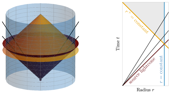
Figure 8: Left: Different choices for the surface $\Sigma$, where the blue surface corresponds to $r=\textrm{constant}$ while the gold surface corresponds to $r^{+}=\textrm{constant}$. The red surface is the light cone corresponding to the perturbation. Right: Cross-section of this configuration for fixed $\mathbf{n}$. Signals from the perturbation (black lines) eventually cross both surfaces: $r=\textrm{constant}$ (blue) and $r^{+}=\textrm{constant}$ (gold). Eq. (A.9) shows equality of the fluxes integrated over either the gold or blue line bounding the gray shaded region.

The radial light cone coordinates introduced in section 2, offer another natural definition of $J$. That is by integrating over the surface $\Sigma_{2}$, defined by $r^{+}=$ constant and depicted by the golden cone in Fig. (8). In the limit $r^{+}\to\infty$ eq. (A.2) becomes

$$Q=\lim_{r^{+}\to\infty}\bigg{(}\frac{r^{+}}{2}\bigg{)}^{d-2}\frac{1}{2}\int_{-\infty}^{+\infty}dr^{-}\int d\Omega_{d-2}\,J^{r^{+}}(r^{+},r^{-},\mathbf{n}).$$ (A.6)

Now, the surfaces $\Sigma_{1}$ and $\Sigma_{2}$ for respectively $r\to\infty$ and $r^{+}\to\infty$ approach $\mathscr{I}^{+}$. While on the plane, this horizon is singular, one can use Weyl invariance to map the charges and current to the Lorentzian cylinder, where $\mathscr{I}^{+}$ is not singular. The currents are therefore smooth on this surface and all components scale similarly. The scaling of the currents at $r^{+}\to\infty$ is hence entirely fixed by the change of coordinate from the cylinder to the plane, and this implies $\lim_{r^{+}\to\infty}J^{r^{-}}/J^{r^{+}}=\lim_{r^{+}\to\infty}J^{\perp}/J^{r^{+}}=0$. Moreover, using current conservation, one can obtain the scaling of the dominant term $J^{r^{+}}$ with $r^{+}$: $\lim_{r^{+}\to\infty}(r^{+}/2)^{d-2}J^{r^{+}}=2j(r^{-},{\mathbf{n}})$ with $j$ a function independent of $r^{+}$. This is confirmed by our computation as well as by the study of the three-point function, which is completely fixed by conformal invariance. Synthesizing: on $\mathscr{I}^{+}$ only the one component of the current, $J^{r^{+}}\equiv J_{r_{-}}$, survives and up to a trivial scaling with $r_{+}$ it is described by a function $j(r^{-},{\mathbf{n}})$.

The above result implies asymptotically

$$r^{d-2}n^{i}J^{i}(t,r{\mathbf{n}})\equiv r^{d-2}J^{r}(t,r{\mathbf{n}})=\left(\frac{2r}{2r+r^{-}}\right)^{d-2}j(t-r,{\mathbf{n}})\xrightarrow{\lim_{r\to\infty}}j(t-r,{\mathbf{n}})$$ (A.7)

and, consequently

$$\mathcal{Q}({\mathbf{n}}) \equiv \lim_{r^{+}\to\infty}\bigg{(}\frac{r^{+}}{2}\bigg{)}^{d-2}\frac{1}{2}\int_{-\infty}^{+\infty}dr^{-}\,J^{r^{+}}(r^{+},r^{-},\mathbf{n})=\lim_{r\to\infty}r^{d-2}\int_{0}^{+\infty}dt\,n^{i}J^{i}(t,r\mathbf{n})$$ (A.8)

$$= \int_{-\infty}^{+\infty}dr^{-}j(r^{-},{\mathbf{n}})\,.$$ (A.9)

This is stronger than the equality of the two expressions for the charge in eqs. (A.5) and (A.6): the time-integrated fluxes at each point on the celestial sphere coincide. All this is consistent with the fact that $\mathscr{I}^{+}$ is not a singular surface in a conformal field theory and thus its integrated flux is independent of the way this surface is approached.

We can now consider the computation using $y$ coordinates. For $t\approx r\to\infty$ (or equivalently, $y^{+}\to 0^{-}$), we have the relation

$$t=\frac{1}{2}\bigg{(}\frac{1+|\vec{y}^{\perp}|^{2}}{-y^{+}}+y^{-}\bigg{)},\quad r=\frac{1}{2}\bigg{(}\frac{1+|\vec{y}^{\perp}|^{2}}{-y^{+}}-\bigg{(}\frac{1-|\vec{y}^{\perp}|^{2}}{1+|\vec{y}^{\perp}|^{2}}\bigg{)}y^{-}\bigg{)},$$ (A.10)

or equivalently,

$$r^{+}=\frac{1+|\vec{y}^{\perp}|^{2}}{-y^{+}}-\bigg{(}\frac{|\vec{y}^{\perp}|^{2}}{1+|\vec{y}^{\perp}|^{2}}\bigg{)}y^{-}\approx\frac{1+|\vec{y}^{\perp}|^{2}}{-y^{+}},\quad r^{-}=\frac{y^{-}}{1+|\vec{y}^{\perp}|^{2}}.$$ (A.11)

Under this change of coordinates, our definition for the charge flux, both in terms of $t$ and $r^{-}$ becomes

$$\mathcal{Q}(\mathbf{n}) =\lim_{y^{+}\to 0^{-}}\bigg{(}\frac{1+|\vec{y}^{\perp}|^{2}}{-2y^{+}}\bigg{)}^{d-2}\int_{-\infty}^{\infty}\frac{dy^{-}}{1+|\vec{y}^{\perp}|^{2}}\cdot(-y^{+})^{d-2}(1+|\vec{y}^{\perp}|^{2})J_{-}(y^{+},y^{-},\vec{y}^{\perp})$$ (A.12)

$$=\bigg{(}\frac{1+|\vec{y}^{\perp}|^{2}}{2}\bigg{)}^{d-2}\int_{-\infty}^{\infty}dy^{-}\,J_{-}(y^{+}=0,y^{-},\vec{y}^{\perp}),$$

Taking into account the relation

$$\vec{n}^{\perp}=\bigg{(}\frac{2}{1+|\vec{y}^{\perp}|^{2}}\bigg{)}\vec{y}^{\perp},$$ (A.13)

we can express the integral over the celestial sphere in terms of $\vec{y}^{\perp}$ as

$$d\Omega_{d-2}=\bigg{(}\frac{2}{1+|\vec{y}^{\perp}|^{2}}\bigg{)}^{d-2}d\vec{y}^{\perp},$$ (A.14)

which guarantees the normalization

$$Q=\int dy^{-}d\vec{y}^{\perp}\mspace{1.0mu}J_{-}(y^{+}=0,y^{-},\vec{y}^{\perp}).$$ (A.15)

For completeness, we show how the mapping works for the energy, in which case we have

$$E=\int\hbox to0.0pt{$\displaystyle\overbrace{\phantom{d\Omega_{d-2}\,\bigg{(}\frac{1+|\vec{y}^{\perp}|^{2}}{2}\bigg{)}^{d-2}}}^{d\vec{y}^{\perp}}$\hss}d\Omega_{d-2}\underbrace{\bigg{(}\frac{1+|\vec{y}^{\perp}|^{2}}{2}\bigg{)}^{d-2}\,\bigg{(}\frac{1+|\vec{y}^{\perp}|^{2}}{2}\bigg{)}\,\overbrace{2\int dy^{-}\,T_{--}(y^{+}=0,y^{-},y^{\perp})}^{\mathcal{E}(\vec{y}^{\perp})}}_{\mathcal{E}(\mathbf{n})}.$$ (A.16)

Appendix B Details of Flux Correlator Computation

In this appendix, we present various details of the calculation of flux operator correlators, both for the free scalar and the semiclassical analysis for more general CFTs.

B.1 Free Theory Calculation in Position Space

As discussed in section 3, there are two contributions to both the charge flux two-point function $\langle\mathcal{Q}\mathcal{Q}\rangle$ and the energy flux two-point function $\langle\mathcal{E}\mathcal{E}\rangle$, corresponding to diagrams $(a)$ and $(b)$ in Figure 3. The $U(1)$ current correlation function corresponding to diagram $(a)$ is

$$\langle\bar{\phi}^{n}(y_{f})\mspace{1.0mu}J_{-}(y_{1})\mspace{1.0mu}J_{-}(y_{2})\mspace{1.0mu}\phi^{n}(y_{i})\rangle^{(a)}$$ (B.1)

$$\quad=n^{2}(n-1)^{2}\mspace{2.0mu}\langle\bar{\phi}(y_{f})\mspace{1.0mu}J_{-}(y_{1})\mspace{1.0mu}\phi(y_{i})\rangle\mspace{2.0mu}\langle\bar{\phi}(y_{f})\mspace{1.0mu}J_{-}(y_{2})\mspace{1.0mu}\phi(y_{i})\rangle\mspace{2.0mu}\langle\bar{\phi}^{n-2}(y_{f})\mspace{1.0mu}\phi^{n-2}(y_{i})\rangle$$

$$\quad=(-1)^{1-d-n(\frac{d-2}{2})}\frac{n!}{\big{(}(d-2)\Omega_{d-1}\big{)}^{n}}\frac{n(n-1)}{(2\Omega_{d-1})^{2}}\frac{y_{fi}^{(2-n)(d-2)}}{y_{f1}^{d-2}y_{1i}^{d-2}y_{f2}^{d-2}y_{2i}^{d-2}}\bigg{(}\frac{y_{f1}^{+}}{y_{f1}^{2}}+\frac{y_{1i}^{+}}{y_{1i}^{2}}\bigg{)}\bigg{(}\frac{y_{f2}^{+}}{y_{f2}^{2}}+\frac{y_{2i}^{+}}{y_{2i}^{2}}\bigg{)},$$

while the current correlation function for diagram (b) is

$$\langle\bar{\phi}^{n}(y_{f})\mspace{1.0mu}J_{-}(y_{1})\mspace{1.0mu}J_{-}(y_{2})\mspace{1.0mu}\phi^{n}(y_{i})\rangle^{(b)}$$ (B.2)

$$\qquad=n^{2}\mspace{2.0mu}\langle\bar{\phi}(y_{f})\mspace{1.0mu}J_{-}(y_{1})J_{-}(y_{2})\mspace{1.0mu}\phi(y_{i})\rangle\mspace{2.0mu}\langle\bar{\phi}^{n-1}(y_{f})\mspace{1.0mu}\phi^{n-1}(y_{i})\rangle$$

$$\qquad=(-1)^{1-d-n(\frac{d-2}{2})}\frac{n!}{\big{(}(d-2)\Omega_{d-1}\big{)}^{n}}\frac{n}{(2\Omega_{d-1})^{2}}\frac{y_{fi}^{(1-n)(d-2)}}{y_{f1}^{d-2}y_{12}^{d-2}y_{2i}^{d-2}}$$

$$\qquad\qquad\times\Bigg{(}\bigg{(}\frac{y_{f1}^{+}}{y_{f1}^{2}}+\frac{y_{12}^{+}}{y_{12}^{2}}\bigg{)}\bigg{(}\frac{y_{12}^{+}}{y_{12}^{2}}+\frac{y_{2i}^{+}}{y_{2i}^{2}}\bigg{)}+\bigg{(}\frac{2}{d-2}\bigg{)}\frac{(y_{12}^{+})^{2}}{y_{12}^{4}}\Bigg{)}.$$

To obtain the resulting charge flux correlator, we need to integrate over $y_{1}^{-}$ and $y_{2}^{-}$ for both of these expressions. Starting with diagram $(a)$, we see that eq. (B.1) factorizes into independent functions of $y_{1}$ and $y_{2}$, such that we have

$$\langle\bar{\phi}^{n}(y_{f})\mspace{1.0mu}\mathcal{Q}(\vec{y}_{1}^{\perp})\mspace{1.0mu}\mathcal{Q}(\vec{y}_{2}^{\perp})\mspace{1.0mu}\phi^{n}(y_{i})\rangle^{(a)}$$ (B.3)

$$\quad=n^{2}(n-1)^{2}\mspace{2.0mu}\langle\bar{\phi}(y_{f})\mspace{1.0mu}\mathcal{Q}(\vec{y}_{1}^{\perp})\mspace{1.0mu}\phi(y_{i})\rangle\mspace{2.0mu}\langle\bar{\phi}(y_{f})\mspace{1.0mu}\mathcal{Q}(\vec{y}_{2}^{\perp})\mspace{1.0mu}\phi(y_{i})\rangle\mspace{2.0mu}\langle\bar{\phi}^{n-2}(y_{f})\mspace{1.0mu}\phi^{n-2}(y_{i})\rangle.$$

We therefore just need to evaluate the integral

$$\langle\bar{\phi}^{n}(y_{f})\mspace{1.0mu}\mathcal{Q}(\vec{y}_{j}^{\perp})\mspace{1.0mu}\phi^{n}(y_{i})\rangle=\frac{(-1)^{\frac{3}{2}-d}}{2(d-2)\Omega^{2}_{d-1}}\int dy_{j}^{-}\frac{1}{y_{fj}^{d-2}y_{ji}^{d-2}}\bigg{(}\frac{y_{fj}^{+}}{y_{fj}^{2}}+\frac{y_{ji}^{+}}{y_{ji}^{2}}\bigg{)}.$$ (B.4)

The integrand has two poles, corresponding to the points along the integral where $y_{j}$ crosses the light cone of $y_{i}$ or $y_{f}$. Due to the Wightman ordering of this correlator, the pole associated with $y_{i}$ is in the upper half-plane while the pole associated with $y_{f}$ is in the lower half-plane. We can therefore close the integration contour in either direction and obtain the resulting expression

$$\langle\bar{\phi}(y_{f})\mspace{1.0mu}\mathcal{Q}(\vec{y}_{j}^{\perp})\mspace{1.0mu}\phi(y_{i})\rangle=\frac{(-1)^{2-d}\mspace{1.0mu}2^{d-2}}{(d-2)\Omega_{d-1}\Omega_{d-2}}\frac{1}{(y_{fj}^{+})^{\frac{d-2}{2}}\mspace{1.0mu}(y_{ji}^{+})^{\frac{d-2}{2}}\mspace{1.0mu}\Big{(}y_{fi}^{-}-\frac{|\vec{y}_{fj}^{\perp}|^{2}}{y_{fj}^{+}}-\frac{|\vec{y}_{ji}^{\perp}|^{2}}{y_{ji}^{+}}\Big{)}^{d-2}},$$ (B.5)

which we can map to $x$-coordinates with the conformal transformation from eq. (2.2),

$$\langle\bar{\phi}(x_{f})\mspace{1.0mu}\mathcal{Q}(\mathbf{n}_{j})\mspace{1.0mu}\phi(x_{i})\rangle=\frac{(-1)^{\frac{2-d}{2}}}{(d-2)\Omega_{d-1}\Omega_{d-2}}\frac{1}{(n_{j}\cdot x_{fi})^{d-2}}.$$ (B.6)

We therefore obtain the full expression for diagram $(a)$,

$$\langle\bar{\phi}^{n}(x_{f})\mspace{1.0mu}\mathcal{Q}(\mathbf{n}_{1})\mspace{1.0mu}\mathcal{Q}(\mathbf{n}_{2})\mspace{1.0mu}\phi^{n}(x_{i})\rangle^{(a)}$$ (B.7)

$$\qquad=(-1)^{n(\frac{2-d}{2})}\frac{n!}{\big{(}(d-2)\Omega_{d-1}\big{)}^{n}}\frac{n(n-1)}{\Omega_{d-2}^{2}}\frac{x_{fi}^{(2-n)(d-2)}}{(n_{1}\cdot x_{fi})^{d-2}\mspace{1.0mu}(n_{2}\cdot x_{fi})^{d-2}}.$$

Turning to the contribution from diagram $(b)$, we see that eq. (B.2) does not factorize into a product of three-point functions. We instead need to compute

$$\langle\bar{\phi}^{n}(y_{f})\mspace{1.0mu}\mathcal{Q}(\vec{y}_{1}^{\perp})\mspace{1.0mu}\mathcal{Q}(\vec{y}_{2}^{\perp})\mspace{1.0mu}\phi^{n}(y_{i})\rangle^{(b)}=n^{2}\mspace{2.0mu}\langle\bar{\phi}(y_{f})\mspace{1.0mu}\mathcal{Q}(\vec{y}_{1}^{\perp})\mspace{1.0mu}\mathcal{Q}(\vec{y}_{2}^{\perp})\mspace{1.0mu}\phi(y_{i})\rangle\mspace{2.0mu}\langle\bar{\phi}^{n-1}(y_{f})\mspace{1.0mu}\phi^{n-1}(y_{i})\rangle,$$ (B.8)

which contains the double integral

$$\langle\bar{\phi}(y_{f})\mspace{1.0mu}\mathcal{Q}(\vec{y}_{1}^{\perp})\mspace{1.0mu}\mathcal{Q}(\vec{y}_{2}^{\perp})\mspace{1.0mu}\phi(y_{i})\rangle$$ (B.9)

$$=\frac{(-1)^{2-\frac{3}{2}d}}{4(d-2)\Omega_{d-1}^{3}}\!\int\!dy_{1}^{-}\!\int\!dy_{2}^{-}\frac{1}{y_{f1}^{d-2}y_{12}^{d-2}y_{2i}^{d-2}}\Bigg{(}\!\bigg{(}\frac{y_{f1}^{+}}{y_{f1}^{2}}+\frac{y_{12}^{+}}{y_{12}^{2}}\bigg{)}\bigg{(}\frac{y_{12}^{+}}{y_{12}^{2}}+\frac{y_{2i}^{+}}{y_{2i}^{2}}\bigg{)}+\bigg{(}\frac{2}{d-2}\bigg{)}\frac{(y_{12}^{+})^{2}}{y_{12}^{4}}\Bigg{)}.$$

The simplest way to evaluate these integrals is to close the contour for $y_{1}^{-}$ in the lower half-plane (picking up the pole from $y_{f}$) and close the contour for $y_{2}^{-}$ in the upper half-plane (picking up the pole from $y_{i}$), such that we obtain

$$\langle\bar{\phi}(y_{f})\mspace{1.0mu}\mathcal{Q}(\vec{y}_{1}^{\perp})\mspace{1.0mu}\mathcal{Q}(\vec{y}_{2}^{\perp})\mspace{1.0mu}\phi(y_{i})\rangle$$ (B.10)

$$\qquad=\frac{(-1)^{2-d}2^{d-2}}{(d-2)\Omega_{d-1}\Omega_{d-2}}\frac{1}{(y_{f1}^{+})^{\frac{d-2}{2}}\mspace{1.0mu}(y_{1i}^{+})^{\frac{d-2}{2}}\mspace{1.0mu}\Big{(}y_{fi}^{-}-\frac{|\vec{y}_{f1}^{\perp}|^{2}}{y_{f1}^{+}}-\frac{|\vec{y}_{1i}^{\perp}|^{2}}{y_{1i}^{+}}\Big{)}^{d-2}}\,\delta(\vec{y}_{12}^{\perp}).$$

Using the relation

$$\bigg{(}\frac{1+|\vec{y}^{\perp}|^{2}}{2}\bigg{)}^{2-d}\delta(\vec{y}^{\perp})=\delta(\mathbf{n}),$$ (B.11)

we can map this expression to $x$-coordinates,

$$\langle\bar{\phi}(x_{f})\mspace{1.0mu}\mathcal{Q}(\mathbf{n}_{1})\mspace{1.0mu}\mathcal{Q}(\mathbf{n}_{2})\mspace{1.0mu}\phi(x_{i})\rangle=\frac{(-1)^{\frac{2-d}{2}}}{(d-2)\Omega_{d-1}\Omega_{d-2}}\frac{1}{(n_{1}\cdot x_{fi})^{d-2}}\,\delta(\mathbf{n}_{1}-\mathbf{n}_{2}).$$ (B.12)

We thus find the resulting expression for diagram $(b)$,

$$\langle\bar{\phi}^{n}(x_{f})\mspace{1.0mu}\mathcal{Q}(\mathbf{n}_{1})\mspace{1.0mu}\mathcal{Q}(\mathbf{n}_{2})\mspace{1.0mu}\phi^{n}(x_{i})\rangle^{(b)}$$ (B.13)

$$\qquad=(-1)^{n(\frac{2-d}{2})}\frac{n!}{\big{(}(d-2)\Omega_{d-1}\big{)}^{n}}\frac{n}{\Omega_{d-2}}\frac{x_{fi}^{(1-n)(d-2)}}{(n_{1}\cdot x_{fi})^{d-2}}\,\delta(\mathbf{n}_{1}-\mathbf{n}_{2}).$$

This particular diagram therefore only contributes if $\mathbf{n}_{1}=\mathbf{n}_{2}$. Intuitively, this is because both insertions of $\mathcal{Q}$ are “measuring” the same free particle, which can only occur if they’re located at the same point on the celestial sphere.

This exact same procedure can be repeated for the energy flux correlator, resulting in the contribution

$$\langle\bar{\phi}^{n}(x_{f})\mspace{1.0mu}\mathcal{E}(\mathbf{n}_{1})\mspace{1.0mu}\mathcal{E}(\mathbf{n}_{2})\mspace{1.0mu}\phi^{n}(x_{i})\rangle^{(a)}$$ (B.14)

$$\qquad=(-1)^{n(\frac{2-d}{2})-1}\frac{n!}{\big{(}(d-2)\Omega_{d-1}\big{)}^{n}}\frac{n(n-1)(d-2)^{2}}{\Omega_{d-2}^{2}}\frac{x_{fi}^{(2-n)(d-2)}}{(n_{1}\cdot x_{fi})^{d-1}\mspace{1.0mu}(n_{2}\cdot x_{fi})^{d-1}},$$

from diagram $(a)$ and

$$\langle\bar{\phi}^{n}(x_{f})\mspace{1.0mu}\mathcal{E}(\mathbf{n}_{1})\mspace{1.0mu}\mathcal{E}(\mathbf{n}_{2})\mspace{1.0mu}\phi^{n}(x_{i})\rangle^{(b)}$$ (B.15)

$$\qquad=(-1)^{n(\frac{2-d}{2})-1}\frac{n!}{\big{(}(d-2)\Omega_{d-1}\big{)}^{n}}\frac{n(d-2)^{2}}{\Omega_{d-2}}\frac{x_{fi}^{(1-n)(d-2)}}{(n_{1}\cdot x_{fi})^{d-1}}\mspace{1.0mu}\delta(\mathbf{n}_{1}-\mathbf{n}_{2}),$$

from diagram $(b)$.

B.2 Fourier Transform to Momentum Space

Once we’ve obtained a flux operator correlation function in position space, we need to Fourier transform with respect to the positions $x_{i}$ and $x_{f}$ of the external operators to obtain the desired momentum space expectation value. Based on the structure of the $k$-point function in eq. (4.18), we must evaluate the general Fourier transform

$$F_{k}^{(\alpha,\beta)}(\mathbf{n}_{1},\ldots,\mathbf{n}_{k};p)\equiv\int d^{d}x\,e^{ip\cdot x}\frac{1}{x^{2\alpha}\mspace{1.0mu}(n_{1}\cdot x)^{\beta}\mspace{1.0mu}\cdots\mspace{1.0mu}(n_{k}\cdot x)^{\beta}}.$$ (B.16)

Our strategy will be to evaluate this expression recursively with the convolution theorem. We therefore need to first evaluate the Fourier transforms of the individual terms

$$f_{\alpha}(p)\equiv\int d^{d}x\,\frac{e^{ip\cdot x}}{\big{(}(x^{+}-i\epsilon)(x^{-}-i\epsilon)-|\vec{x}^{\perp}|^{2}\big{)}^{\alpha}}=\frac{(-1)^{\alpha}\pi^{\frac{d+2}{2}}p^{2\alpha-d}}{2^{2\alpha-d-1}\Gamma(\alpha)\Gamma(\alpha-\frac{d-2}{2})}\Theta(p_{0})\Theta(p^{2}),$$ (B.17)

and

$$g_{\beta}(\mathbf{n};p)\equiv\int d^{d}x\,\frac{e^{ip\cdot x}}{(n\cdot x)^{\beta}}=\frac{(2\pi)^{d}}{\Gamma(\beta)}p_{0}^{\beta-1}\delta(\mathbf{p}-p_{0}\mathbf{n})\,\Theta(p_{0}),$$ (B.18)

where $\Theta(x)$ is the Heaviside step function.

Using these building blocks, we can evaluate the Fourier transform for $k=1$,

$$F_{1}^{(\alpha,\beta)}(\mathbf{n};p) =\int\frac{d^{d}q}{(2\pi)^{d}}\,f_{\alpha}(p-q)\,g_{\beta}(\mathbf{n};q)$$ (B.19)

$$=\frac{1}{\Gamma(\beta)}\int_{0}^{\frac{p^{2}}{2n\cdot p}}\!dq_{0}\,q_{0}^{\beta-1}f_{\alpha}(p-q_{0}n)$$

$$=\frac{(-1)^{\alpha}\pi^{\frac{d+2}{2}}}{2^{2\alpha+\beta-d-1}\Gamma(\alpha)\Gamma(\alpha+\beta-\frac{d-2}{2})}\frac{p^{2(\alpha+\beta)-d}}{(n\cdot p)^{\beta}}\Theta(p_{0})\Theta(p^{2}),$$

where we have used the fact that $f_{\alpha}(p-q)\propto\Theta\big{(}(p-q)^{2}\big{)}$ to limit the integral over $q_{0}$ to a finite range.

We can then apply the convolution theorem again to obtain the Fourier transform of $k=2$ for the simplified case where $p^{\mu}=(E,\mathbf{0})$

$$F_{2}^{(\alpha,\beta)}(\mathbf{n}_{1},\mathbf{n}_{2};E)=\frac{1}{\Gamma(\beta)}\int_{0}^{\frac{E}{2}}\!dq_{0}\,q_{0}^{\beta-1}F_{1}^{(\alpha,\beta)}(\mathbf{n}_{1};p-q_{0}n_{2})$$ (B.20)

$$\qquad=\frac{(-1)^{\alpha}\pi^{\frac{d+2}{2}}E^{2\alpha+2\beta-d}}{2^{2\alpha+2\beta-d-1}\Gamma(\alpha)\Gamma(\alpha+2\beta-\frac{d-2}{2})}\,{}_{2}F_{1}\big{(}\beta,\beta;\alpha+2\beta-\tfrac{d-2}{2};\tfrac{n_{1}\cdot n_{2}}{2}\big{)}\,\Theta(E).$$

Unfortunately, the necessary integrals become increasingly complicated for higher $k$. However, the expression simplifies dramatically if we focus on the limit $\alpha\to\infty$ with $\beta$ and $k$ fixed. Looking at the integral for $k=2$ again (for general $p^{\mu}$), we have

$$F_{2}^{(\alpha,\beta)}(\mathbf{n}_{1},\mathbf{n}_{2};p)$$ (B.21)

$$\qquad=\frac{(-1)^{\alpha}\pi^{\frac{d+2}{2}}}{2^{2\alpha+\beta-d-1}\Gamma(\alpha)\Gamma(\beta)\Gamma(\alpha+\beta-\frac{d-2}{2})}\int_{0}^{\frac{p^{2}}{2n_{2}\cdot p}}\!dq_{0}\,\frac{q_{0}^{\beta-1}(p^{2}-2q_{0}\mspace{1.0mu}n_{2}\cdot p)^{\alpha+\beta-\frac{d}{2}}}{(n_{1}\cdot p-q_{0}\mspace{1.0mu}n_{1}\cdot n_{2})^{\beta}}.$$

If we interpret the factor of $(p^{2}-2q_{0}\mspace{1.0mu}n_{2}\cdot p)^{\alpha+\beta-\frac{d}{2}}$ as an overall derivative and integrate by parts, the boundary terms both vanish due to the positive powers of $q_{0}$ and $p^{2}-2q_{0}\mspace{1.0mu}n_{2}\cdot p$, leaving us with the new integral

$$\int_{0}^{\frac{p^{2}}{2n_{2}\cdot p}}\!dq_{0}\,\frac{q_{0}^{\beta-1}(p^{2}-2q_{0}\mspace{1.0mu}n_{2}\cdot p)^{\alpha+\beta-\frac{d}{2}}}{(n_{1}\cdot p-q_{0}\mspace{1.0mu}n_{1}\cdot n_{2})^{\beta}}$$ (B.22)

$$\quad=\frac{1}{2\mspace{1.0mu}n_{2}\cdot p(\alpha+\beta-\frac{d-2}{2})}\int_{0}^{\frac{p^{2}}{2n_{2}\cdot p}}\!dq_{0}\,\bigg{(}(\beta-1)\frac{q_{0}^{\beta-2}(p^{2}-2q_{0}\mspace{1.0mu}n_{2}\cdot p)^{\alpha+\beta-\frac{d-2}{2}}}{(n_{1}\cdot p-q_{0}\mspace{1.0mu}n_{1}\cdot n_{2})^{\beta}}$$

$$\hskip 199.16928pt+\,\beta\mspace{1.0mu}n_{1}\cdot n_{2}\mspace{1.0mu}\frac{q_{0}^{\beta-1}(p^{2}-2q_{0}\mspace{1.0mu}n_{2}\cdot p)^{\alpha+\beta-\frac{d-2}{2}}}{(n_{1}\cdot p-q_{0}\mspace{1.0mu}n_{1}\cdot n_{2})^{\beta+1}}\bigg{)}.$$

As we can see, each integration by parts brings down an overall factor of $1/\alpha$. The leading contribution as $\alpha\to\infty$ will therefore come from the fewest actions of integration by parts that lead to a non-vanishing boundary term, which is obtained by repeatedly acting with derivatives on the initial power of $q_{0}^{\beta-1}$ in the numerator until its exponent vanishes (as $\beta$ is a positive integer). We thus find the leading behavior at large $\alpha$:

$$F_{2}^{(\alpha,\beta)}(\mathbf{n}_{1},\mathbf{n}_{2};p)\approx\frac{(-1)^{\alpha}\pi^{\frac{d+2}{2}}}{2^{2\alpha+2\beta-d-1}\Gamma(\alpha)\Gamma(\alpha+2\beta-\frac{d-2}{2})}\frac{p^{2\alpha+4\beta-d}}{(n_{1}\cdot p)^{\beta}\mspace{1.0mu}(n_{2}\cdot p)^{\beta}}\Big{(}1+O(1/\alpha)\Big{)}.$$ (B.23)

We can apply this same analysis recursively to higher values of $k$, obtaining the general leading order behavior

$$F_{k}^{(\alpha,\beta)}(\mathbf{n}_{1},\ldots,\mathbf{n}_{k};p)\approx\frac{(-1)^{\alpha}\pi^{\frac{d+2}{2}}}{2^{2\alpha+k\beta-d-1}\Gamma(\alpha)\Gamma(\alpha+k\beta-\frac{d-2}{2})}\frac{p^{2\alpha+2k\beta-d}}{(n_{1}\cdot p)^{\beta}\mspace{1.0mu}\cdots\mspace{1.0mu}(n_{k}\cdot p)^{\beta}}\quad(\alpha\to\infty).$$ (B.24)

The next-to-leading order correction comes from acting with one derivative on any of the factors of $(n_{i}\cdot p-q_{0}\mspace{1.0mu}n_{i}\cdot n_{j})^{\beta+1}$ in the denominator while integrating by parts and is, therefore, $O(k^{2}/\alpha)$ relative to the leading behavior (with a suppression of $1/\alpha$ due to the extra derivative and an enhancement of $k(k-1)$ due to combinatorics).

B.3 Map from the Cylinder to the Plane

In order to use the semiclassical approach of [11, 12] for the calculation of flux operators, including subleading corrections, we need to map expectation values on the Euclidean cylinder to correlation functions on the Euclidean plane. Here we’ll present the details of this mapping, focusing mainly on the two-point function of the $U(1)$ current $J_{\mu}$ before discussing the generalization to higher-point functions and correlators of $T_{\mu\nu}$.

Our starting point is the cylinder four-point function from eq. (4.12):

$$\frac{\langle Q|\mspace{1.0mu}J^{\mu}(\tau_{1},\vec{N}_{1})\mspace{1.0mu}J^{\nu}(\tau_{2},\vec{N}_{2})\mspace{1.0mu}|Q\rangle}{\langle Q|Q\rangle}=-\bigg{(}\frac{Q}{\Omega_{d-1}}\bigg{)}^{2}\delta^{\mu}_{\,\tau}\delta^{\nu}_{\,\tau}.$$ (B.25)

Because all four operators are primary, we can use the Weyl transformation in eq. (2.7) to obtain the correlator on the plane

$$\frac{\langle\overline{\mathcal{O}}_{Q}(\infty)\mspace{1.0mu}J^{\mu}(y_{1})\mspace{1.0mu}J^{\nu}(y_{2})\mspace{1.0mu}\mathcal{O}_{Q}(0)\rangle}{\langle\overline{\mathcal{O}}_{Q}(\infty)\mspace{1.0mu}\mathcal{O}_{Q}(0)\rangle} =e^{-(d-1)(\tau_{1}+\tau_{2})}\mspace{1.0mu}\frac{\langle Q|\mspace{1.0mu}J^{\mu}(\tau_{1},\vec{N}_{1})\mspace{1.0mu}J^{\nu}(\tau_{2},\vec{N}_{2})\mspace{1.0mu}|Q\rangle}{\langle Q|Q\rangle}$$ (B.26)

$$=-\bigg{(}\frac{Q}{\Omega_{d-1}}\bigg{)}^{2}\frac{y_{1}^{\mu}}{y_{1}^{d}}\frac{y_{2}^{\nu}}{y_{2}^{d}}.$$

We now need to perform a conformal transformation to move the external operators away from zero and infinity to arbitrary positions $y_{i}$ and $y_{f}$. The most systematic way to do this is to decompose this correlation function in terms of the basis of tensor structures allowed by conformal symmetry. For a four-point function with two scalar operators and two insertions of the $U(1)$ current, there are five independent structures, allowing us to write any such correlator in the general form [52]

$$\frac{\langle\overline{\mathcal{O}}_{Q}(y_{f})\mspace{1.0mu}J^{\mu}(y_{1})\mspace{1.0mu}J^{\nu}(y_{2})\mspace{1.0mu}\mathcal{O}_{Q}(y_{i})\rangle}{\langle\overline{\mathcal{O}}_{Q}(y_{f})\mspace{1.0mu}\mathcal{O}_{Q}(y_{i})\rangle} =\frac{1}{y_{12}^{2d}}\bigg{(}g_{0}(u,v)H_{12}^{\mu\nu}+g_{1}(u,v)V^{\mu}_{1,fi}V^{\nu}_{2,fi}+g_{2}(u,v)V^{\mu}_{1,fi}V^{\nu}_{2,1i}$$ (B.27)

$$\hskip 42.67912pt+\,g_{3}(u,v)V^{\mu}_{1,f2}V^{\nu}_{2,fi}+g_{4}(u,v)V^{\mu}_{1,f2}V^{\nu}_{2,1i}\bigg{)},$$

where the tensor structures are defined as

$$H_{ab}^{\mu\nu}\equiv y_{ab}^{2}\mspace{1.0mu}g^{\mu\nu}-2y_{ab}^{\mu}\mspace{1.0mu}y_{ab}^{\nu},\qquad V^{\mu}_{a,bc}\equiv\frac{y_{ab}^{2}\mspace{1.0mu}y_{ac}^{2}}{y_{bc}^{2}}\bigg{(}\frac{y_{ab}^{\mu}}{y_{ab}^{2}}-\frac{y_{ac}^{\mu}}{y_{ac}^{2}}\bigg{)},$$ (B.28)

and the various coefficients $g_{a}(u,v)$ are theory-dependent functions of the conformal invariant cross-ratios

$$u=\frac{y_{f1}^{2}\mspace{1.0mu}y_{2i}^{2}}{y_{f2}^{2}\mspace{1.0mu}y_{1i}^{2}},\qquad v=\frac{y_{fi}^{2}\mspace{1.0mu}y_{12}^{2}}{y_{f2}^{2}\mspace{1.0mu}y_{1i}^{2}}.$$ (B.29)

We can determine the functions $g_{a}(u,v)$ by taking the limit $y_{i}\to 0$, $y_{f}\to\infty$ of the general four-point function in eq. (B.27) and matching it to our semiclassical result in eq. (B.26). In this limit, the tensor structures and cross-ratios take the simpler form

$$V^{\mu}_{a,fi}\to-y_{a}^{\mu},\quad V^{\mu}_{1,f2}\to-y_{12}^{\mu},\quad V^{\mu}_{2,1i}\to-\frac{y_{12}^{2}\mspace{1.0mu}y_{2}^{2}}{y_{1}^{2}}\bigg{(}\frac{y_{12}^{\mu}}{y_{12}^{2}}+\frac{y_{2}^{\mu}}{y_{2}^{2}}\bigg{)},\quad u\to\frac{y_{2}^{2}}{y_{1}^{2}},\quad v\to\frac{y_{12}^{2}}{y_{1}^{2}}.$$ (B.30)

From this limiting behavior, we can rewrite eq. (B.26) in the manifestly conformally covariant form

$$\frac{\langle\overline{\mathcal{O}}_{Q}(\infty)\,J^{\mu}(y_{1})J^{\nu}(y_{2})\,\mathcal{O}_{Q}(0)\rangle}{\langle\overline{\mathcal{O}}_{Q}(\infty)\mathcal{O}_{Q}(0)\rangle}=-\bigg{(}\frac{Q}{\Omega_{d-1}}\bigg{)}^{2}\frac{1}{y_{12}^{2d}}\frac{v^{d}}{u^{\frac{d}{2}}}V_{1,fi}^{\mu}V_{2,fi}^{\nu},$$ (B.31)

from which we can read off the functions

$$g_{1}(u,v)=\frac{v^{d}}{u^{\frac{d}{2}}},\quad g_{0}(u,v)=g_{2}(u,v)=g_{3}(u,v)=g_{4}(u,v)=0.$$ (B.32)

We can now evaluate this Euclidean four-point function for any location of the external operators,

$$\frac{\langle\overline{\mathcal{O}}_{Q}(y_{f})\mspace{1.0mu}J^{\mu}(y_{1})\mspace{1.0mu}J^{\nu}(y_{2})\mspace{1.0mu}\mathcal{O}_{Q}(y_{i})\rangle}{\langle\overline{\mathcal{O}}_{Q}(y_{f})\mspace{1.0mu}\mathcal{O}_{Q}(y_{i})\rangle}=-\bigg{(}\frac{Q}{\Omega_{d-1}}\bigg{)}^{2}\frac{y_{fi}^{2(d-2)}}{y_{f2}^{d-2}y_{1i}^{d-2}y_{f1}^{d-2}y_{2i}^{d-2}}\bigg{(}\frac{y_{f1}^{\mu}}{y_{f1}^{2}}+\frac{y_{1i}^{\mu}}{y_{1i}^{2}}\bigg{)}\bigg{(}\frac{y_{f2}^{\mu}}{y_{f2}^{2}}+\frac{y_{2i}^{\mu}}{y_{2i}^{2}}\bigg{)}.$$ (B.33)

While this result for the leading behavior is simple, corresponding to the product of three-point functions $\langle\overline{\mathcal{O}}_{Q}J^{\mu}\mathcal{O}_{Q}\rangle\langle\overline{\mathcal{O}}_{Q}J^{\nu}\mathcal{O}_{Q}\rangle$, this same approach of decomposition in terms of tensor structures can be applied to more complicated expressions arising from subleading corrections in the large charge expansion, allowing us to readily translate Euclidean correlators on the cylinder to Lorentzian correlators on the plane.

We can also extend this procedure to Euclidean correlators with $k$ insertions of the conserved current, with the similar semiclassical result at large $Q$,

$$\frac{\langle\overline{\mathcal{O}}_{Q}(\infty)\mspace{1.0mu}J^{\mu_{1}}(y_{1})\mspace{1.0mu}\cdots\mspace{1.0mu}J^{\mu_{k}}(y_{k})\mspace{1.0mu}\mathcal{O}_{Q}(0)\rangle}{\langle\overline{\mathcal{O}}_{Q}(\infty)\mspace{1.0mu}\mathcal{O}_{Q}(0)\rangle}=(-1)^{\frac{k}{2}}\bigg{(}\frac{Q}{\Omega_{d-1}}\bigg{)}^{k}\frac{y_{1}^{\mu_{1}}}{y_{1}^{d}}\cdots\frac{y_{k}^{\mu_{k}}}{y_{k}^{d}}.$$ (B.34)

While the set of possible tensor structures is more complicated for higher $k$, for the leading behavior as $Q\to\infty$ we again find that only one combination contributes to this correlator,

$$\frac{\langle\overline{\mathcal{O}}_{Q}(\infty)\mspace{1.0mu}J^{\mu_{1}}(y_{1})\mspace{1.0mu}\cdots\mspace{1.0mu}J^{\mu_{k}}(y_{k})\mspace{1.0mu}\mathcal{O}_{Q}(0)\rangle}{\langle\overline{\mathcal{O}}_{Q}(\infty)\mspace{1.0mu}\mathcal{O}_{Q}(0)\rangle}\propto V_{1,fi}^{\mu_{1}}\mspace{1.0mu}\cdots\mspace{1.0mu}V_{k,fi}^{\mu_{k}},$$ (B.35)

allowing us to reconstruct this correlation function for arbitrary $y_{i}$ and $y_{f}$.

Finally, we can consider correlation functions involving the stress-energy tensor, such as the four-point function

$$\frac{\langle\overline{\mathcal{O}}_{Q}(\infty)\mspace{1.0mu}T^{\mu\nu}(y_{1})\mspace{1.0mu}T^{\rho\sigma}(y_{2})\mspace{1.0mu}\mathcal{O}_{Q}(0)\rangle}{\langle\overline{\mathcal{O}}_{Q}(\infty)\mspace{1.0mu}\mathcal{O}_{Q}(0)\rangle}=\bigg{(}\frac{d\Delta_{Q}}{(d-1)\Omega_{d-1}}\bigg{)}^{2}\bigg{(}\frac{y_{1}^{\mu}\mspace{1.0mu}y_{1}^{\nu}}{y_{1}^{2d+2}}-\frac{1}{d}\frac{g^{\mu\nu}}{y_{1}^{2d}}\bigg{)}\bigg{(}\frac{y_{2}^{\rho}\mspace{1.0mu}y_{2}^{\sigma}}{y_{2}^{2d+2}}-\frac{1}{d}\frac{g^{\rho\sigma}}{y_{2}^{2d}}\bigg{)}.$$ (B.36)

We can again write down all possible tensor structures built from $H_{ab}^{\mu\nu}$ and $V_{a,bc}^{\mu}$ and match that general expression to this particular correlator. Fortunately, just like for the $U(1)$ current, this semiclassical expression factorizes into a product of three-point functions, allowing us to obtain the simple result

$$\frac{\langle\overline{\mathcal{O}}_{Q}(y_{f})\mspace{1.0mu}T^{\mu\nu}(y_{1})\mspace{1.0mu}T^{\rho\sigma}(y_{2})\mspace{1.0mu}\mathcal{O}_{Q}(y_{i})\rangle}{\langle\overline{\mathcal{O}}_{Q}(y_{f})\mspace{1.0mu}\mathcal{O}_{Q}(y_{i})\rangle}$$ (B.37)

$$\qquad=\bigg{(}\frac{d\Delta_{Q}}{(d-1)\Omega_{d-1}}\bigg{)}^{2}\frac{1}{y_{12}^{2d+2}}\frac{v^{d+1}}{u^{\frac{d+1}{2}}}\bigg{(}V_{1,fi}^{\mu}V_{1,fi}^{\nu}-\frac{1}{d}V_{1,fi}^{2}\mspace{1.0mu}g^{\mu\nu}\bigg{)}\bigg{(}V_{2,fi}^{\rho}V_{2,fi}^{\sigma}-\frac{1}{d}V_{2,fi}^{2}\mspace{1.0mu}g^{\rho\sigma}\bigg{)},$$

with an analogous expression for $k$ insertions of the stress tensor.

References

- [1] P. W. Anderson, “More Is Different,” Science 177 no. 4047, (1972) 393–396.
- [2] J. M. Cornwall, “On the High-energy Behavior of Weakly Coupled Gauge Theories,” Phys. Lett. B 243 (1990) 271–278.
- [3] H. Goldberg, “Breakdown of perturbation theory at tree level in theories with scalars,” Phys. Lett. B 246 (1990) 445–450.
- [4] M. B. Voloshin, “Multiparticle amplitudes at zero energy and momentum in scalar theory,” Nucl. Phys. B 383 (1992) 233–248.
- [5] L. S. Brown, “Summing tree graphs at threshold,” Phys. Rev. D 46 (1992) R4125–R4127, arXiv:hep-ph/9209203.
- [6] M. B. Voloshin, “Summing one loop graphs at multiparticle threshold,” Phys. Rev. D 47 (1993) R357–R361, arXiv:hep-ph/9209240.
- [7] M. V. Libanov, V. A. Rubakov, D. T. Son, and S. V. Troitsky, “Exponentiation of multiparticle amplitudes in scalar theories,” Phys. Rev. D 50 (1994) 7553–7569, arXiv:hep-ph/9407381.
- [8] D. T. Son, “Semiclassical approach for multiparticle production in scalar theories,” Nucl. Phys. B 477 (1996) 378–406, arXiv:hep-ph/9505338.
- [9] V. A. Rubakov, “Nonperturbative aspects of multiparticle production,” in 2nd Rencontres du Vietnam: Physics at the Frontiers of the Standard Model. 1995. arXiv:hep-ph/9511236.
- [10] S. Demidov, B. Farkhtdinov, and D. Levkov, “Numerical Study of Multiparticle Production in 4 Theory,” Phys. Part. Nucl. Lett. 20 no. 3, (2023) 229–232, arXiv:2307.11163 [hep-ph].
- [11] S. Hellerman, D. Orlando, S. Reffert, and M. Watanabe, “On the CFT Operator Spectrum at Large Global Charge,” JHEP 12 (2015) 071, arXiv:1505.01537 [hep-th].
- [12] A. Monin, D. Pirtskhalava, R. Rattazzi, and F. K. Seibold, “Semiclassics, Goldstone Bosons and CFT data,” JHEP 06 (2017) 011, arXiv:1611.02912 [hep-th].
- [13] L. Alvarez-Gaume, O. Loukas, D. Orlando, and S. Reffert, “Compensating strong coupling with large charge,” JHEP 04 (2017) 059, arXiv:1610.04495 [hep-th].
- [14] G. Cuomo, A. de la Fuente, A. Monin, D. Pirtskhalava, and R. Rattazzi, “Rotating superfluids and spinning charged operators in conformal field theory,” Phys. Rev. D 97 no. 4, (2018) 045012, arXiv:1711.02108 [hep-th].
- [15] D. Banerjee, S. Chandrasekharan, and D. Orlando, “Conformal dimensions via large charge expansion,” Phys. Rev. Lett. 120 no. 6, (2018) 061603, arXiv:1707.00711 [hep-lat].
- [16] A. De La Fuente, “The large charge expansion at large ,” JHEP 08 (2018) 041, arXiv:1805.00501 [hep-th].
- [17] G. Badel, G. Cuomo, A. Monin, and R. Rattazzi, “The Epsilon Expansion Meets Semiclassics,” JHEP 11 (2019) 110, arXiv:1909.01269 [hep-th].
- [18] O. Antipin, J. Bersini, F. Sannino, Z.-W. Wang, and C. Zhang, “Charging the model,” Phys. Rev. D 102 no. 4, (2020) 045011, arXiv:2003.13121 [hep-th].
- [19] G. Badel, G. Cuomo, A. Monin, and R. Rattazzi, “Feynman diagrams and the large charge expansion in dimensions,” Phys. Lett. B 802 (2020) 135202, arXiv:1911.08505 [hep-th].
- [20] G. Arias-Tamargo, D. Rodriguez-Gomez, and J. G. Russo, “Correlation functions in scalar field theory at large charge,” JHEP 01 (2020) 171, arXiv:1912.01623 [hep-th].
- [21] G. Cuomo, “A note on the large charge expansion in 4d CFT,” Phys. Lett. B 812 (2021) 136014, arXiv:2010.00407 [hep-th].
- [22] G. Cuomo, L. V. Delacretaz, and U. Mehta, “Large Charge Sector of 3d Parity-Violating CFTs,” JHEP 05 (2021) 115, arXiv:2102.05046 [hep-th].
- [23] G. Cuomo, “OPE meets semiclassics,” Phys. Rev. D 103 no. 8, (2021) 085005, arXiv:2103.01331 [hep-th].
- [24] G. Cuomo, M. Mezei, and A. Raviv-Moshe, “Boundary conformal field theory at large charge,” JHEP 10 (2021) 143, arXiv:2108.06579 [hep-th].
- [25] N. Dondi, I. Kalogerakis, R. Moser, D. Orlando, and S. Reffert, “Spinning correlators in large-charge CFTs,” Nucl. Phys. B 983 (2022) 115928, arXiv:2203.12624 [hep-th].
- [26] G. Badel, A. Monin, and R. Rattazzi, “Identifying Large Charge operators,” JHEP 02 (2023) 119, arXiv:2207.08919 [hep-th].
- [27] G. Cuomo and Z. Komargodski, “Giant Vortices and the Regge Limit,” JHEP 01 (2023) 006, arXiv:2210.15694 [hep-th].
- [28] G. Cuomo, J. M. V. P. Lopes, J. Matos, J. Oliveira, and J. Penedones, “Numerical tests of the large charge expansion,” arXiv:2305.00499 [hep-lat].
- [29] D. M. Hofman and J. Maldacena, “Conformal collider physics: Energy and charge correlations,” JHEP 05 (2008) 012, arXiv:0803.1467 [hep-th].
- [30] G. P. Korchemsky and G. F. Sterman, “Power corrections to event shapes and factorization,” Nucl. Phys. B 555 (1999) 335–351, arXiv:hep-ph/9902341.
- [31] A. V. Belitsky, S. Hohenegger, G. P. Korchemsky, E. Sokatchev, and A. Zhiboedov, “From correlation functions to event shapes,” Nucl. Phys. B 884 (2014) 305–343, arXiv:1309.0769 [hep-th].
- [32] A. V. Belitsky, S. Hohenegger, G. P. Korchemsky, E. Sokatchev, and A. Zhiboedov, “Event shapes in super-Yang-Mills theory,” Nucl. Phys. B 884 (2014) 206–256, arXiv:1309.1424 [hep-th].
- [33] A. V. Belitsky, S. Hohenegger, G. P. Korchemsky, E. Sokatchev, and A. Zhiboedov, “Energy-Energy Correlations in N=4 Supersymmetric Yang-Mills Theory,” Phys. Rev. Lett. 112 no. 7, (2014) 071601, arXiv:1311.6800 [hep-th].
- [34] T. Hartman, S. Kundu, and A. Tajdini, “Averaged Null Energy Condition from Causality,” JHEP 07 (2017) 066, arXiv:1610.05308 [hep-th].
- [35] C. Cordova, J. Maldacena, and G. J. Turiaci, “Bounds on OPE Coefficients from Interference Effects in the Conformal Collider,” JHEP 11 (2017) 032, arXiv:1710.03199 [hep-th].
- [36] P. Kravchuk and D. Simmons-Duffin, “Light-ray operators in conformal field theory,” JHEP 11 (2018) 102, arXiv:1805.00098 [hep-th].
- [37] A. Belin, D. M. Hofman, and G. Mathys, “Einstein gravity from ANEC correlators,” JHEP 08 (2019) 032, arXiv:1904.05892 [hep-th].
- [38] M. Kologlu, P. Kravchuk, D. Simmons-Duffin, and A. Zhiboedov, “Shocks, Superconvergence, and a Stringy Equivalence Principle,” JHEP 11 (2020) 096, arXiv:1904.05905 [hep-th].
- [39] M. Kologlu, P. Kravchuk, D. Simmons-Duffin, and A. Zhiboedov, “The light-ray OPE and conformal colliders,” JHEP 01 (2021) 128, arXiv:1905.01311 [hep-th].
- [40] K.-W. Huang, “Lightcone Commutator and Stress-Tensor Exchange in CFTs,” Phys. Rev. D 102 no. 2, (2020) 021701, arXiv:2002.00110 [hep-th].
- [41] C.-H. Chang, M. Kologlu, P. Kravchuk, D. Simmons-Duffin, and A. Zhiboedov, “Transverse spin in the light-ray OPE,” JHEP 05 (2022) 059, arXiv:2010.04726 [hep-th].
- [42] A. Belin, D. M. Hofman, G. Mathys, and M. T. Walters, “On the stress tensor light-ray operator algebra,” JHEP 05 (2021) 033, arXiv:2011.13862 [hep-th].
- [43] G. P. Korchemsky, E. Sokatchev, and A. Zhiboedov, “Generalizing event shapes: in search of lost collider time,” JHEP 08 (2022) 188, arXiv:2106.14899 [hep-th].
- [44] G. P. Korchemsky and A. Zhiboedov, “On the light-ray algebra in conformal field theories,” JHEP 02 (2022) 140, arXiv:2109.13269 [hep-th].
- [45] D. Chicherin, G. P. Korchemsky, E. Sokatchev, and A. Zhiboedov, “Energy correlations in heavy states,” arXiv:2306.14330 [hep-th].
- [46] P. T. Komiske, I. Moult, J. Thaler, and H. X. Zhu, “Analyzing N-Point Energy Correlators inside Jets with CMS Open Data,” Phys. Rev. Lett. 130 no. 5, (2023) 051901, arXiv:2201.07800 [hep-ph].
- [47] K. Lee, B. Mecaj, and I. Moult, “Conformal Colliders Meet the LHC,” arXiv:2205.03414 [hep-ph].
- [48] T. Hartman, S. Jain, and S. Kundu, “Causality Constraints in Conformal Field Theory,” JHEP 05 (2016) 099, arXiv:1509.00014 [hep-th].
- [49] A. Nicolis, R. Penco, F. Piazza, and R. Rattazzi, “Zoology of condensed matter: Framids, ordinary stuff, extra-ordinary stuff,” JHEP 06 (2015) 155, arXiv:1501.03845 [hep-th].
- [50] E. Firat, A. Monin, F. Nardi, R. Rattazzi, and M. T. Walters. Work in progress.
- [51] S. Giombi and J. Hyman, “On the large charge sector in the critical O(N) model at large N,” JHEP 09 (2021) 184, arXiv:2011.11622 [hep-th].
- [52] M. S. Costa, J. Penedones, D. Poland, and S. Rychkov, “Spinning Conformal Correlators,” JHEP 11 (2011) 071, arXiv:1107.3554 [hep-th].