Finite Pulse-Time Effects in Long-Baseline Quantum Clock Interferometry

Abstract

Quantum-clock interferometry has been suggested as a quantum probe to test the universality of free fall (UFF) and the universality of gravitational redshift (UGR). In typical experimental schemes it seems advantageous to employ Doppler-free E1-M1 transitions which have so far been investigated in quantum gases at rest. Here, we consider the fully quantized atomic degrees of freedom and study the interplay of the quantum center-of-mass (COM) – that can become delocalized – together with the internal clock transitions. In particular, we derive a model for finite-time E1-M1 transitions with atomic intern-extern coupling and arbitrary position-dependent laser intensities. We further provide generalizations to the ideal expressions for perturbed recoilless clock pulses. Finally, we show at the example of a Gaussian laser beam that the proposed quantum-clock interferometers are stable against perturbations from varying optical fields for a sufficiently small quantum delocalization of the atomic COM.

I Introduction

Light-pulse atom interferometry (LPAI) has demonstrated its versatility in a myriad of applications: Starting from measuring gravitational acceleration Kasevich and Chu (1991); Peters, Chung, and Chu (1998); Peters et al. (1999) and rotation Lan et al. (2012) to field applications Barrett et al. (2016); Wu et al. (2019); Templier et al. (2022); Stray et al. (2022) and mobile gravimetry Wu et al. (2019), the measurement of Newton’s gravitational constant Rosi et al. (2014) as well as the so-far most accurate determination of the fine structure constant Parker et al. (2018); Morel et al. (2020). In the last decade, there have been proposals for mid-band gravitational wave detection Dimopoulos et al. (2008a, 2009); Graham et al. (2016), complementary to LIGO/VIRGO and LISA, and recently construction has started on first prototypes which might be sensitive to ultra-light dark matter signals Geraci and Derevianko (2016); Arvanitaki et al. (2018); Badurina et al. (2023) and serve as testbeds for gravitational wave antennas Abe et al. (2021); Bertoldi et al. (2021); Badurina, Blas, and McCabe (2022) based on atom interferometry.

These advancements have paved the way to perform tests on the fundamental physical principles underlying today’s best physical theories with high precision atomic sensors Safronova et al. (2018); Dimopoulos et al. (2007, 2008b); Asenbaum et al. (2020). On the other hand, ever-increasing precision goals require an upscaling of the interferometers’ spacetime areas. For that reason, several very-large baseline projects are currently being planned globally, hoping to reach the kilometer scale: AION-km in the UK Badurina et al. (2020), MAGIS-km in the USA Abe et al. (2021), MIGA/ELGAR in Europe Canuel et al. (2018, 2020), and ZAIGA in China Zhan et al. (2019).

A side beneficiary of these endeavors will be new long baseline tests of the Einstein equivalence principle, encapsulated in its three pillars Di Pumpo et al. (2023) consisting of local Lorentz invariance, the universality of free fall (UFF) and local position invariance which in turn contains the universality of gravitational redshift (UGR) and universality of clock rates (UCR). Together these principles form the backbone of general relativity Will (2014); Di Casola, Liberati, and Sonego (2015). All aspects of the equivalence principle have proven to be extremely resilient to experimental challenges over an extremely large regime ranging from the microscopic to the cosmic scale Vessot et al. (1980); Chou et al. (2010); Herrmann et al. (2018); Delva et al. (2019); Takamoto et al. (2020); Bothwell et al. (2022); Brewer et al. (2019); Oelker et al. (2019); Madjarov et al. (2019); Touboul et al. (2019); Schlippert et al. (2014); Archibald et al. (2018); Zheng et al. (2023).

UFF in particular has been tested via LPAI by comparison of the free fall rates of different atomic isotopes and species Schlippert et al. (2014); Asenbaum et al. (2020); Rosi et al. (2017) as well as for different internal states Zhou et al. (2021) of the same atomic species. However, LPAI using quantum clocks as initial states have been shown Loriani et al. (2019) to be insensitive to UGR violations in a linear gravitational field without additional internal transitions during Giulini (2012); Roura (2020); Ufrecht and Giese (2020); Di Pumpo et al. (2021) the interferometer. Recently, two different LPAI schemes were introduced for UGR and UFF tests by Roura Roura (2020) and Ufrecht et al. Ufrecht et al. (2020) In contrast to the original proposals by Zych et al. Zych et al. (2011) and Sinha et al. Sinha and Samuel (2011) to detect general relativistic time dilation by the interference of quantum clocks in a gravitational field, both proposals are predicated on the essential step of initializing the atomic clock inside the interferometer in order to unequivocally isolate such a signal. Without this crucial step one is stuck with the no-go result Loriani et al. (2019). Therefore the scheme of Roura Roura (2020) needs a superposition of internal states to gain UGR sensitivity (and being insensitive to UFF violations); the alternative approach of Ufrecht et al. Ufrecht et al. (2020) does not require superpositions of internal states (as seen by the laboratory frame). In turn it becomes sensitive to both, UGR and UFF violations. Similarly, other proposals Di Pumpo et al. (2021, 2023) can test different aspects of local position invariance like UCR.

Ideally one would like to initialize an atomic clock inside the interferometer without disturbing the center-of-mass (COM) motion of the atomic test masses which serve as inertial reference. Hence, recoilless internal transitions are strongly beneficial or might even be necessary since they can ease the experimental constraints and the implementation significantly. In this study, we examine recoilless transitions implemented via two-photon E1-M1 couplings, i.e. two-photon transitions consisting of one electric dipole (E1) and one magnetic dipole (M1) transition. This type of two-photon process has previously been investigated for Doppler-free two-photon spectroscopy Grynberg (1983); Rahaman, Wright, and Dutta (2023) and for the application in optical atomic vapor clocks Alden, Moore, and Leanhardt (2014); Alden (2014) without COM motion. In contrast to these previous studies, we will consider the full quantum nature of all atomic degrees of freedom – internal and COM. Due to the quantized nature of the COM degrees of freedom one would a priori expect that the LPAI phase shift suffers from the corresponding delocalizing light-matter interaction Lopp and Martín-Martínez (2021). In particular, we find after incorporating COM motion that additional momentum kicks and thus branches appear when considering realistic spatial laser profiles. However, we show that the protocols of Roura Roura (2020) and Ufrecht et al. Ufrecht et al. (2020) are resilient to leading order effects in the induced COM spread when compared to the interferometer size. Nonetheless, our results can serve as a guide when such or similar corrections need to be accounted for or modeled in future high precision experiments.

Overview & Structure

Our article is structured as follows: In Sec. II we will recapitulate the two interferometer schemes presented by Roura Roura (2020) and Ufrecht et al. Ufrecht et al. (2020), and put them into the context of the dynamical mass energy of composite particles. In Sec. III we will introduce an idealized model for E1-M1 transitions using plane waves for the electromagnetic field. The internal structure of the atom will be described by a three-level system that can be reduced to an effective two-level system using adiabatic elimination. To achieve the absorption of two counter-propagating photons a specific polarization scheme is needed Alden, Moore, and Leanhardt (2014); Alden (2014). In Sec. IV we will extend these results and include the finite pulse-time effects for E1-M1 transitions using a more realistic model, i.e. taking into account position-dependent laser intensities. The generalized $\pi$- and $\pi/2$-pulse operators will be obtained in Sec. IV.1 for the experimentally relevant case of a Gaussian laser beam. In Sec. V we will come back to the two interferometer schemes Roura (2020); Ufrecht et al. (2020) and analyze the implications due to the finite pulse times, in particular their impact on the phase and visibility of the interferometers. We conclude with a summary, discussion and contextualization of our results in Sec. VI.

II UGR and UFF tests with Quantum Clock Interferometry

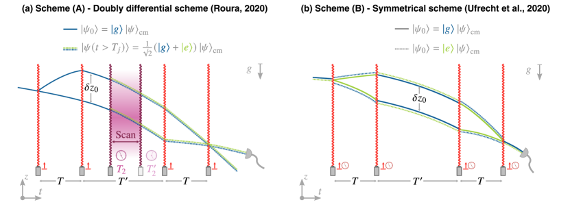
FIG. 1: Two LPAI proposals utilizing atomic clocks to detect UGR and UFF violations. Panel (a) Scheme (A) is doubly differential: The atom enters the interferometer sequence in the ground state $\ket{g}$ and is split up onto two branches, e.g. via a Bragg pulse. At time $T_{2}$ a recoilless E1-M1 pulse drives the atom into a superposition of excited (denoted by $\ket{e}$) and ground state, corresponding to the initialization of an atomic clock. The branches are recombined afterwards and one can measure the intensities in the ground and excited state channels. The experiment is then repeated with a different initialization time $T_{2}^{\prime}=T_{2}+\tau$. The COM wave function is denoted by $\ket{\psi}_{\text{cm}}$. Panel (b) Scheme (B) on the other hand is symmetrical: The atom enters the interferometer sequence in the ground/excited state and is split up onto two branches, e.g. via a double Bragg diffraction pulse. In the middle segment, in between the times $t=T$ and $t=T+T^{\prime}$, the internal state is changed to the excited/ground state via a recoilless E1-M1 transition. After recombining the two branches the detection is performed. A single run of the experiment consists of two runs of the interferometer sequence with different initial internal states.

Here, we will briefly review the two interferometer schemes Roura (2020); Ufrecht et al. (2020) employing quantum clocks to test UGR and UFF. In the following we will denote the scheme proposed by Roura Roura (2020) as scheme (A) and the one proposed by Ufrecht et al. Ufrecht et al. (2020) as scheme (B). Before starting this discussion we will introduce the relevant aspects of the dynamical mass energy (or mass defect) of atoms which is the underlying connection to test the UGR and UFF in an interferometer with quantum clocks. We note that our introduction only serves as a sketch of the ingredients necessary for incorporating a description of dynamical mass energy perturbatively into atoms.

While Einstein’s mass energy equivalence $E=Mc^{2}$ has been known for more than 100 years now, its impact on quantum interference due to the possibility of obtaining which-path information for composite particles with time-evolving internal structure has only recently been highlighted in the works of Zych et al. Zych et al. (2011) and Sinha et al. Sinha and Samuel (2011) How dynamical mass energy manifests in a Mach-Zehnder atom interferometer was first sketched by Giulini Giulini (2012) in the context of the redshift debate Müller, Peters, and Chu (2010a, b); Wolf et al. (2010, 2011, 2012); Schleich, Greenberger, and Rasel (2013). Based on these initial considerations, significant progress has been made. For a review of these initial discussions and proposed experiments beyond the ones discussed here Roura (2020); Ufrecht et al. (2020) see e.g. the works of Pikovski et al. Pikovski et al. (2017) or Di Pumpo et al. Di Pumpo et al. (2021) and references therein.

However, to the authors’ knowledge, dynamical mass energy itself was already discussed in the works of Sebastian Sebastian (1981, 1986) on semi-relativistic models for composite systems interacting with a radiation field. There the author indicates that the appearance of these terms (including dynamical mass energy) is intimately linked to relativistic corrections to the COM coordinates first derived by Osborn et al. Osborn (1968); Close and Osborn (1970) and Krajcik et al. Krajcik and Foldy (1974) over 50 years ago. The last few years have seen significant efforts and discussions devoted to providing first principles derivations from atomic physics of dynamical mass energy. Specifically, we refer to the works of Sonnleitner et al. Sonnleitner and Barnett (2018) and Schwartz et al. Schwartz and Giulini (2019); Schwartz (2020) for systems with quantized COM motion, respectively without and with gravity. A field theoretical derivation has recently been performed by Aßmann et al. Aßmann, Giese, and Di Pumpo (2023) Moreover Perche et al. Perche and Neuser (2021); Perche (2022) contains a discussion under which conditions and by which guiding principles effective models for composite systems can be constructed in curved spacetime. Extensions examining the coupling of Dirac particles to gravitational backgrounds have recently also been discussed Ito (2021); Perche and Neuser (2021); Alibabaei, Schwartz, and Giulini (2023) yielding overall sensible but in the details slightly differing results in the weak-field limit. A general review discussing the issues and problems regarding such couplings of quantum matter to gravity is available in Guilini et al. Giulini, Großardt, and Schwartz (2022)

II.1 A Simple Model for the Dynamical Mass Energy of Atoms

In the non-relativistic limit, a first-quantized Hamiltonian description of a particle of mass $M$ moving in a weak gravitational field is prescribed Anastopoulos and Hu (2018) by the sum of the kinetic COM energy and its gravitational potential energy $U(\boldsymbol{\mathbf{R}})$

$$\hat{H}(\hat{\boldsymbol{\mathbf{R}}},\hat{\boldsymbol{\mathbf{P}}};M)=Mc^{2}+MU(\hat{\boldsymbol{\mathbf{R}}})+\frac{\hat{\boldsymbol{\mathbf{P}}}^{2}}{2M}-\frac{\hat{\boldsymbol{\mathbf{P}}}U(\hat{\boldsymbol{\mathbf{R}}})\hat{\boldsymbol{\mathbf{P}}}}{2M},$$ (1)

with COM position $\hat{\vec{R}}$ and momentum $\hat{\boldsymbol{\mathbf{P}}}$ where we have neglected any terms contributing at orders higher than $1/M$. Practically, the gravitational potential can often be approximated as $U(\hat{\vec{R}})=U(\boldsymbol{\mathbf{R}}_{0})+\boldsymbol{\mathbf{g}}^{\intercal}(\hat{\boldsymbol{\mathbf{R}}}-\boldsymbol{\mathbf{R}}_{0})+(\hat{\boldsymbol{\mathbf{R}}}-\boldsymbol{\mathbf{R}}_{0})^{\intercal}\Gamma(\hat{\boldsymbol{\mathbf{R}}}-\boldsymbol{\mathbf{R}}_{0})/2$ up to the gravity gradient contribution where we adopted a symmetric Weyl ordering for the operators $\hat{\boldsymbol{\mathbf{R}}}$ and $\hat{\boldsymbol{\mathbf{P}}}$ and have expanded around the point $\vec{R}_{0}$ in whose vicinity the system is localized. Note, that the mass $M$ of the particle corresponds to its rest mass here. Hence, only in going beyond this non-relativistic model, the dynamical nature of mass energy can become relevant.

When considering the atom to be comprised of individual particles sub-leading relativistic corrections will appear Sebastian (1981, 1986); Pikovski et al. (2017); Schwartz and Giulini (2019); Schwartz (2020); Martínez-Lahuerta et al. (2022); Wood and Zych (2022) and change the Hamiltonian. The most impactful change resulting from this is the insight that the total atomic mass is no longer just the sum of the rest masses of its constituent particles but also contains a contribution from the internal Hamiltonian of the atom, as one would naively expect from mass energy equivalence. We incorporate this in our simple model by performing the replacement Schwartz (2020)

$$M\mapsto\hat{M}=M+\frac{\hat{H}_{\mathrm{A}}}{c^{2}}.$$ (2)

Note, that we have introduced the abbreviation $\hat{M}$ for the quantity $\hat{M}=M+\hat{H}_{A}/c^{2}$ which behaves akin to a mass operator. In this we are guided by the fact that the eigenvalue equation $\hat{M}\ket{n}=M_{n}\ket{n}$ leads to the eigenvalues $\mathcal{E}_{j}$ of the internal Hamiltionian $\hat{H}_{A}$. These are determined by the eigenvalue equation $\hat{H}_{A}\ket{n}=\mathcal{E}_{n}\ket{n}$ and directly connected to the eigenvalues of the mass operator $M_{n}=M+\mathcal{E}_{j}/c^{2}$, that is they are scaled by the square of the speed of light and shifted by the rest mass. Since there is a one-to-one mapping between the eigenvalues and eigenstates of the the mass operator and the internal Hamiltionian no additional complexity of the system in terms of additional Hilbert spaces or new dynamics is gained, and to this order this looks like a simple reformulation in terms of different quantities.

Furthermore, if the smallest and largest eigenstate of the internal Hamiltonian $\hat{H}_{A}$ are separated by an energy $\Delta\mathcal{E}\ll Mc^{2}$, then the intern-extern coupling can be treated perturbatively. This is a useful approximation e.g. in the case of optical clock transitions in ytterbium or strontium where the (relevant part of the) internal Hamiltonian has a spectral range in the optical regime and we can thus estimateLoriani et al. (2019) $\|\hat{H}_{A}\|/(Mc^{2})\leavevmode\nobreak\ \simeq\leavevmode\nobreak\ 10^{-11}$. Thus, often we can assume the perturbative identification Loriani et al. (2019) $M^{-1}\big{(}1-\hat{H}_{A}/(Mc^{2})\big{)}\simeq M^{-1}\big{(}1+\hat{H}_{A}/(Mc^{2})\big{)}^{-1}$ via the geometric series. Consequently, we can also replace $M^{-1}\mapsto\hat{M}^{-1}$ in the terms in Eq. (1) describing the potential and kinetic energy. The overall Hamiltonian $\hat{H}^{(\text{MD})}$, including the mass defect, accordingly takes the form

$$\begin{split}\hat{H}^{(\text{MD})}=\hat{H}(\hat{\boldsymbol{\mathbf{R}}},\hat{\boldsymbol{\mathbf{P}}};\hat{M})=\hat{M}c^{2}+\hat{M}U(\hat{\boldsymbol{\mathbf{R}}})+\frac{\hat{\boldsymbol{\mathbf{P}}}^{2}}{2\hat{M}}-\frac{\hat{\boldsymbol{\mathbf{P}}}U(\hat{\boldsymbol{\mathbf{R}}})\hat{\boldsymbol{\mathbf{P}}}}{2\hat{M}}.\end{split}$$ (3)

All but the first term in Eq. (3) induce a coupling of the internal atomic energies to the kinetic and potential energy of the COM.

Alternatively, using the energy eigenstates $\ket{n}$ and the mass operator eigenvalues $M_{n}=M+\mathcal{E}_{n}/c^{2}$, the Hamiltonian $\hat{H}^{(\text{MD})}$ can be rewritten as

$$\hat{H}^{(\text{ME})}=\sum_{n}\hat{H}^{\text{(ME)}}_{n}\outerproduct{n}{n}\quad\text{with}\leavevmode\nobreak\ \hat{H}^{\text{(ME)}}_{n}=\hat{H}(\hat{\boldsymbol{\mathbf{R}}},\hat{\boldsymbol{\mathbf{P}}};M_{n}),$$ (4)

which is equivalent to a collection of single particles, characterized by the state-dependent masses $M_{n}$. In this form the Hamiltonian directly embodies the equivalence of inertial and gravitational mass Anastopoulos and Hu (2018). While we have omitted the coupling to external (electromagnetic) fields in all our considerations for simplicity, they are in principle instrumental to actually prepare and manipulate the atomic wave packet in experiments. These may be accounted for in an interaction Hamiltonian $\hat{H}_{\text{int}}$ added to Eq. (3) or Eq. (4), since the mass eigenstates are identical to the internal energy eigenstates except for an energy shift. The details of this interaction Hamiltonian can be quite complicated Sonnleitner and Barnett (2018); Schwartz (2020); Aßmann, Giese, and Di Pumpo (2023) when all corrections from the mass defect are included. However, to leading order it consists of the standard electric or magnetic dipole transitions described by

$$\hat{H}_{\text{int}}=-\hat{\boldsymbol{\mathbf{d}}}\cdot\boldsymbol{\mathbf{E}}(t,\hat{\boldsymbol{\mathbf{R}}})+\hat{\boldsymbol{\mathbf{\mu}}}\cdot\boldsymbol{\mathbf{B}}(t,\hat{\boldsymbol{\mathbf{R}}}),$$ (5)

where $\hat{\boldsymbol{\mathbf{d}}}$ and $\hat{\boldsymbol{\mathbf{\mu}}}$ are the atomic electric and magnetic dipole operators, respectively. Note that we have neglected here terms to leading order in the electric charge and Bohr radius that are further suppressed by the atomic mass $M$, such as the Röntgen term Lopp and Martín-Martínez (2021). In conclusion we arrive at the total model Hamiltonian (excluding higher order contributions for the electromagnetic field coupling)

$$\hat{\mathcal{H}}=\hat{H}^{\text{(MD)}}+\hat{H}_{\text{int}}=\hat{H}^{\text{(ME)}}+\hat{H}_{\text{int}}$$ (6)

for an atom with internal structure interacting with an external electromagnetic field.

While our introduction here can only serve as a sketch, motivated by mass energy equivalence, it turns out that the derivation of the intern-extern coupling can be made fairly rigorous Anastopoulos and Hu (2018); Loriani et al. (2019); Schwartz and Giulini (2019); Schwartz (2020); Martínez-Lahuerta et al. (2022); Aßmann, Giese, and Di Pumpo (2023), however with serious gains in the theoretical complexity of the model depending on the setting as well as the starting point. Nevertheless, the basic premises and leading order results do not change significantly.

II.2 Phase Shift in a Light-Pulse Atom Interferometer

There are multiple methods available to calculate the phase shift in a LPAI. In simple cases, with quadratic Hamiltonians and for instantaneous beam splitter pulses, one can often rely on path-integral methods Storey and Cohen-Tannoudji (1994). However path-integrals become quite unwieldy in case of non-quadratic systems as there are no or only few standard methods available for their solution Kleinert (2009). In these more involved cases, e.g. with multiple internal states and complicated external potentials involved, the Hamiltonian approach Schleich, Greenberger, and Rasel (2013); Kleinert et al. (2015); Ufrecht (2021) offers a more versatile toolbox. Moreover, phase-space methods Giese et al. (2014); Roura, Zeller, and Schleich (2014); Zimmermann (2021) are also available and sometimes helpful for interpretation.

However, in all cases the interference signal in an exit port of a two-path interferometer arises from the superposition of two branches characterized by the evolutions $\hat{U}_{1}$ and $\hat{U}_{2}$ and is determined by the expectation value Schleich, Greenberger, and Rasel (2013); Di Pumpo et al. (2023)

$$I_{\phi_{\text{exit}}}=\bra{\psi_{0}}\hat{U}_{\text{tot}}^{\dagger}\hat{\Pi}_{\text{exit}}^{\phantom{x}}\hat{U}_{\text{tot}}\ket{\psi_{0}},$$ (7)

with the overall evolution given by $\hat{\Pi}_{\text{exit}}\hat{U}_{\text{tot}}=\hat{U}_{1}+\hat{U}_{2}$. Here $\hat{U}_{\text{tot}}$ is the total time evolution, $\hat{\Pi}_{\text{exit}}$ is a projection operator with the property $\hat{\Pi}_{\text{exit}}^{2}=\hat{\Pi}_{\text{exit}}$ characteristic to the detection process occurring in the exit port and $\ket{\psi_{0}}$ is the initial state at the start of the interferometer. Note that here the individual evolutions $\hat{U}_{1}$ and $\hat{U}_{2}$ need not be unitary by themselves. In fact, even in a Mach-Zehnder interferometer they are not. This is due to the fact that only half of the atoms participates in each branch of the interferometer. Furthermore, the individual nature of the beam splitters creating the interferometer decides the balance between the interferometer branches. On the other hand the total evolution $\hat{U}_{\text{tot}}$ usually is unitary, unless e.g. atom losses occur or not all paths are included in the modelling of the interferometer and thus $\hat{U}_{\text{tot}}$ becomes an open system evolution.

After expanding the sum over the individual branches in the exit port signal, defined in Eq. (7), it takes the form

$$\begin{split}I_{\phi_{\text{exit}}}&=\bra{\psi_{0}}\hat{U}_{1}^{\dagger}\hat{U}_{1}^{\phantom{\dagger}}\ket{\psi_{0}}+\bra{\psi_{0}}\hat{U}_{2}^{\dagger}\hat{U}_{2}^{\phantom{\dagger}}\ket{\psi_{0}}\\ &\quad\quad\quad+\bra{\psi_{0}}\hat{\mathcal{O}}\ket{\psi_{0}}+\text{c.c.}\end{split}$$ (8)

where we introduced the amplitude

$$\langle\hat{\mathcal{O}}_{21}\rangle=\bra{\psi_{0}}\hat{U}_{2}^{\dagger}\hat{U}_{1}^{\phantom{\dagger}}\ket{\psi_{0}}=\mathcal{V}_{21}\exp(\text{i}\Delta\phi_{21})$$ (9)

of the so-called overlap operator Schleich, Greenberger, and Rasel (2013)  $\hat{\mathcal{O}}_{21}=\hat{U}_{2}^{\dagger}\hat{U}_{1}^{\phantom{\dagger}}$ between the branches. The absolute value of this amplitude is the visibility $\mathcal{V}_{21}=|\bra{\psi_{0}}\hat{U}_{2}^{\dagger}\hat{U}_{1}^{\phantom{\dagger}}\ket{\psi_{0}}|$ of the interference signal, while the argument $\Delta\phi_{21}=\text{arg}\bra{\psi_{0}}\hat{U}_{2}^{\dagger}\hat{U}_{1}^{\phantom{\dagger}}\ket{\psi_{0}}$ is the interferometer phase Schleich, Greenberger, and Rasel (2013); Ufrecht et al. (2020); Di Pumpo et al. (2023).

In general, the situation in a realistic LPAI can be a bit more complex and the overall signal $I_{\phi_{\text{exit}}}$ detected in an exit port results from the pair-wise interference of all paths through the interferometer contributing to the exit port. Practically, additional and often undesired paths can originate e.g. from imperfect diffraction processes Jenewein et al. (2022); Kirsten-Siemß et al. (2023) or perturbing potentials acting during the interferometer.

However, any interfering pair of paths contributing to the signal amplitude of the exit port in such a multi-path LPAI has a contribution of the form of the expectation value of an overlap

$$I_{\phi_{\text{exit}}}^{(lm)}=\bra{\psi_{0}}\hat{U}^{\dagger}_{\ell}\hat{U}_{m}^{\phantom{x}}\ket{\psi_{0}}+\text{c.c.}=\mathcal{V}_{\ell m}\exp(\text{i}\Delta\phi_{\ell m})+\text{c.c.}$$ (10)

Here we have introduced the relative path visibility $\mathcal{V}_{\ell m}$ and relative phase between paths $\Delta\phi_{\ell m}$ which generalizes the same quantities from the two-path case. Summation over the signal amplitude contributions $I_{\phi_{\text{exit}}}^{(lm)}$ with respect to the indices $\ell$ and $m$ directly leads to the overall exit port signal

$$I_{\phi_{\text{exit}}}=2\sum_{\ell\geq 1}\mathcal{V}_{\ell\ell}+\sum_{\begin{subarray}{c}\ell,m\geq 1\\ \ell\neq m\end{subarray}}\mathcal{V}_{\ell m}\exp(\text{i}\Delta\phi_{\ell m}).$$ (11)

When we also note that the relative phase between paths obeys the relation $\Delta\phi_{\ell m}=-\Delta\phi_{m\ell}$ we arrive at the expression

$$I_{\phi_{\text{exit}}}=2\Big{(}\sum_{\ell}\mathcal{V}_{\ell\ell}+\sum_{\begin{subarray}{c}\ell,m\geq 1\\ \ell\neq m\end{subarray}}\mathcal{V}_{\ell m}\cos\Delta\phi_{\ell m}\Big{)}$$ (12)

for the exit port signal. This expression is a superposition of the cosines of the relative path phases weighted by the relative path visibilities. In an (open) two-path interferometer the sums terminate after two terms, and is thus identical to Eq. (8).

II.3 Interferometer Phase, (Classical) Action and Proper time

Usually, the interferometer phase in a LPAI is linked to the (classical) action by appealing to the relativistic action of a massive particle in a gravitational background Storey and Cohen-Tannoudji (1994); Schleich, Greenberger, and Rasel (2013); Loriani et al. (2019); Di Pumpo et al. (2021) and a subsequent non-relativistic expansion. The resulting expression is then quantized and introduced as governing action $\mathcal{S}$ of an appropriate path integral for the particle. Afterwards one identifies the quantum mechanical phase Loriani et al. (2019) acquired along the trajectory via

$$\phi=-\omega_{C}\tau=-\frac{1}{\hbar}\int\!\!\!\differential t\leavevmode\nobreak\ \mathcal{L}(\boldsymbol{\mathbf{R}},\dot{\boldsymbol{\mathbf{R}}},t)+S_{\text{em}}/\hbar,$$ (13)

where $\omega_{C}=Mc^{2}/\hbar$ is the Compton frequency and $\mathcal{L}$ is the classical Lagrangian $\mathcal{L}(\boldsymbol{\mathbf{R}},\dot{\boldsymbol{\mathbf{R}}})$ corresponding to the Hamiltonian, Eq. (1), of the particle. Here $S_{\text{em}}$ is the action corresponding to the Lagrangian for the electromagnetic interaction, Eq. (5), needed for manipulation of the atom. Fundamentally, this interpretation originates from a semi-classical approximation for the Feynman path-integral Storey and Cohen-Tannoudji (1994); Kleinert (2009) being a valid approximation. This is due to the fact that only in the semi-classical limit the dominant contributions to the path-integral come from the classical trajectories, resulting from solving the Euler-Lagrange equations for the (classical) Lagrangian Kleinert (2009). Ultimately, this is what makes the identification between proper time and the action in Eq. (13) possible also for quantum particles but only in the semi-classical limit.

II.4 UGR Sensitive Scheme (A)

The interferometer scheme (A) Roura (2020), shown in Fig. 1(a), initializes an atomic clock by a recoilless $\pi/2$-pulse so that the atoms that enter the interferometer in the ground state are in a 50:50 superpostion of excited and ground state atoms after the clock initialization. Due to the atoms having a different mass $M_{g,e}$ in their respective internal ground and excited states, the Compton frequency $\omega_{g,e}$ becomes state-dependent. One can measure the frequency in the ground and excited state exit port between the two branches via the differential phase shift $\Delta\phi_{g,e}$ and separate out the gravitational redshift by a double-differential measurement, i.e. calculating the phase difference $\Delta\phi_{-}$ between the excited and ground state exit port and performing two runs of the experiment with different initialization times $T_{2}$ of the atomic clock:

$$\Delta\phi_{-}(T_{2})-\Delta\phi_{-}(T_{2}+\tau)=-\frac{\Delta M}{\bar{M}}gk_{p}\delta T\tau,$$ (14)

where

$$\Delta\phi_{-}(T_{2})=\Delta\phi_{g}(T_{2})-\Delta\phi_{e}(T_{2}),$$ (15)

$\bar{M}=(M_{e}+M_{g})/2$ is the mean mass, $g$ is the gravitational acceleration, $k_{p}$ is the wave number of the laser that drives the atoms onto the two branches, $\delta T$ is the separation time, and $\Delta M=M_{e}-M_{g}$ is the mass difference due to the mass defect. Since the rest mass $M$ and the mean mass $\bar{M}$ are equivalent to our order of approximation, i.e. to order $\mathcal{O}(c^{-2})$ Loriani et al. (2019), we may identify the mean mass as $M$.

II.5 UGR and UFF Sensitive Scheme (B)

The interferometer scheme (B) Ufrecht et al. (2020) (cf. Fig. 1(b)) is sensitive to both, the UGR and UFF. In contrast to scheme (A) it does not require a superpostion of internal states. The sensitivity arises from the specific space-time geometry of the interferometer and a change of internal states so that the atoms are in the same state at equal times (in the laboratory frame). The total phase

$$\Delta\Phi=\Delta\Phi_{M}-\frac{\Delta Mc^{2}}{2\hbar}\sum_{n}\lambda_{\pm}\Delta\tau_{n}$$ (16)

consists of two contributions: the contribution $\Delta\Phi_{M}$ is independent of the mass defect $\Delta M$ and is obtained via the reference Hamiltonian $\hat{H}_{M}$ at the mean mass $M$. This part of the total phase can be used for tests of UFF Ufrecht et al. (2020). The proper time differences $\Delta\tau_{n}$ in each segment $n$ of the interferometer enter the phase proportional to the mass defect $\Delta M$ such that it can be associated with the ticking rate of an atomic clock Di Pumpo et al. (2021). The $\lambda_{\pm}$ indicate the internal state for each segment: $\lambda_{-}=-1$ for the ground state and $\lambda_{+}=+1$ for the excited state. Since the sum $\Delta\tau=\Delta\tau_{1}+\Delta\tau_{2}+\Delta\tau_{3}$ of the proper-time differences vanishes in this geometry, the proper-time difference in the middle segment can be written as $\Delta\tau_{2}=-(\Delta\tau_{1}+\Delta\tau_{3})$. Changing the internal state in the middle segment (associated with $\Delta\tau_{2}$), the total phase becomes

$$\Delta\Phi=\Delta\Phi_{M}\pm\frac{\Delta Mc^{2}}{\hbar}\Delta\tau_{2},$$ (17)

depending on the choice of the initial internal state. Again, performing two runs of the experiment with different initial internal states one can separate the UFF and the UGR effects by adding or subtracting the phases, respectively:

$$\Delta\phi_{+} =2\Delta\phi_{M},$$ (18a)

$$\Delta\phi_{-} =2\frac{\Delta Mc^{2}}{\hbar}\Delta\tau_{2}.$$ (18b)

II.6 Common Challenges

Both interferometer schemes presented above require the manipulation of the internal states during the interferometer sequence. While this manipulation can be achieved by (technically challenging) optical Double-Raman diffraction Sarkar et al. (2022) in scheme (B), i.e. kicking the atoms and changing the internal states simultaneously, scheme (A) requires recoilless internal transitions. There are several reasons why one would like to avoid Double-Raman diffraction: first of all, to drive this kind of transitions one needs quite long laser pulses leading to finite pulse-time effects. Secondly, the single-photon detuning cannot be chosen arbitrarily large if one still wants to have significant Rabi frequencies. This constraint for the detunings leads to problems with spontaneous emision. Furthermore, Double-Raman diffraction requires a high stability for the difference of the two laser frequencies during the pulse. Replacing the Double-Raman diffraction by a momentum-transfer pulse, e.g. Double-Bragg diffraction, and a state-changing pulse could alleviate these issues. These recoilless transitions can be achieved by E1-M1 transitions where the atom absorbs two counter-propagating photons with equal frequency $\omega$ so that the total momentum kick caused by the two-photon transition vanishes. Such E1-M1 transitions were only investigated without (quantized) COM motion in the context of optical clocks Alden, Moore, and Leanhardt (2014); Alden (2014); Zanon-Willette et al. (2023). However, in atom interferometry the COM motion plays a crucial role. Hence, its influence also needs to be included when modeling the pulses to account for possible corrections. This is the task of the following sections.

III Idealized model for E1-M1 transitions

In this section we will derive an effective model for the E1-M1 transition processes during the LPAI schemes discussed in the previous section for an atomic cloud in a gravitational potential, see Fig. 2. The cloud will be modelled as a fully first-quantized atom, including its quantized COM motion. In particular, this can be applied to general initial atomic wavepackets. We will assume, for now, that the electromagnetic fields of the laser beam are classical plane waves. The extension to realistic position-dependent laser intensities and finite pulse-time effects will be treated in Sec. IV.

III.1 Model

For an arbitrary three-level atom of mass $M$ in a gravitational field along $-Z$ and via the dipole approximation the Hamiltonian reads

$$\hat{\tilde{H}}=\frac{\hat{\boldsymbol{\mathbf{P}}}^{2}}{2M}+\sum_{n}\mathcal{E}_{n}\outerproduct{n}{n}-\hat{\boldsymbol{\mathbf{d}}}\cdot\boldsymbol{\mathbf{E}}(t,\hat{\boldsymbol{\mathbf{R}}})+\hat{\boldsymbol{\mathbf{\mu}}}\cdot\boldsymbol{\mathbf{B}}(t,\hat{\boldsymbol{\mathbf{R}}})+Mg\hat{Z},$$ (19)

where $\mathcal{E}_{n}$ are the atomic internal energies. For simplicity, we will assume the electric and magnetic fields, $\boldsymbol{\mathbf{E}}$ and $\boldsymbol{\mathbf{B}}$, to be plane waves with frequency $\omega$ for now. Note that we have neglected the mass defect, cf. Eq. (2), during the interaction with the laser since the pulse time $t$ is much smaller than the characteristic interferometer time $T$. The internal-state dependent mass energy enters the phase via $\Delta Mc^{2}\cdot t/\hbar$ and $\Delta Mc^{2}\cdot T/\hbar$, respectively. The effects of the mass defect during the laser pulse compared to the effects during the rest of the interferometer sequence is therefore negligible. In particular, the $\mathcal{O}(c^{-2})$ correction of Eq. (3) is subdominant with respect to the dipolar interaction terms. Moreover, for the same reason we have only retained the linear potential contribution from the gravitational potential energy and do not consider the higher order contributions due to gravity gradients and kinetic-energy to position couplings from Eq. (79). If necessary they could be included perturbatively, similar to the optical potentials in Sec. IV.

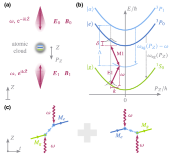
FIG. 2: Panel (a) Incoming and reflected electromagnetic waves with frequency $\omega$ and amplitudes $\boldsymbol{\mathbf{E}}_{i}$ and $\boldsymbol{\mathbf{B}}_{i}$ driving E1-M1 transition in a three-level atom with quantized COM motion (black arrow). Panel (b) Three-level atom with ground state $\ket{g}$, excited state $\ket{e}$ and ancilla state $\ket{a}$ modelled by the states ${}^{1}S_{0}$, ${}^{3}P_{0}$ and ${}^{3}P_{1}$, respectively. Counter-propagating fields drive E1-M1 transitions, i.e. an E1 transition between $\ket{g}$ and $\ket{a}$ with single-photon detuning $\Delta$ and subsequent M1 transition between $\ket{a}$ and $\ket{e}$ leading to the overall detuning $\delta$. The ancilla state $\ket{a}$ lies then virtually between the energy levels of $\ket{g}$ and $\ket{e}$. Panel (c) Left: Two-photon excitation by absorbing two counter-propagating photons with momentum $\pm\hbar\boldsymbol{\mathbf{k}}_{L}$. The first absorption leads to a transition from $\ket{g}$ to $\ket{a}$ and a momentum kick $\hbar\boldsymbol{\mathbf{k}}_{L}$, the second absorption is a transition from $\ket{a}$ to $\ket{e}$ with momentum kick $-\hbar\boldsymbol{\mathbf{k}}_{L}$. Right: Two-photon decay by stimulated emission of two photons in opposite directions. The first emission leads to a transition from $\ket{e}$ to $\ket{a}$ and a momentum kick $-\hbar\boldsymbol{\mathbf{k}}_{L}$ and the second emission is a transition from $\ket{a}$ to $\ket{g}$ with momentum kick $\hbar\boldsymbol{\mathbf{k}}_{L}$. Both two-photon processes have a vanishing netto momentum kick.

In order to describe the laser beam in a retro-reflective geometry, we consider two counter-propagating electromagnetic plane waves. To obtain a recoilless two-photon transition one has to ensure that the atom absorbs two counter-propagating photons. This can be achieved by choice of a certain polarization scheme as we will discuss later on in Sec. III.3; for now we will keep the polarization arbitrary. Then the fields can be written as:

$$\boldsymbol{\mathbf{E}}(\hat{Z}) =\sum_{j=0}^{1}\mathrm{i}\,\boldsymbol{\mathbf{E}}_{j}\mathrm{e}^{(-1)^{j}\mathrm{i}\,k_{L}\hat{Z}}\mathrm{e}^{-\mathrm{i}\,\omega t}+\text{h.c.},$$ (20a)

$$\boldsymbol{\mathbf{B}}(\hat{Z}) =\sum_{j=0}^{1}\mathrm{i}\,\boldsymbol{\mathbf{B}}_{j}\mathrm{e}^{(-1)^{j}\mathrm{i}\,k_{L}\hat{Z}}\mathrm{e}^{-\mathrm{i}\,\omega t}+\text{h.c.}$$ (20b)

We particularize to E1 transitions only between the ground state $\ket{g}$ and the ancilla state $\ket{a}$ and M1 transitions only between the ancilla state $\ket{a}$ and the excited state $\ket{e}$, i.e. the matrix elements $\boldsymbol{\mathbf{d}}_{ea}=\bra{e}\hat{\boldsymbol{\mathbf{d}}}\ket{a}$ and $\boldsymbol{\mathbf{\mu}}_{ag}=\bra{a}\hat{\boldsymbol{\mathbf{\mu}}}\ket{g}$ vanish. This can be ensured by considering the selection rules for electric and magnetic dipole transitions that are discussed subsequently. Thus, in the internal atomic eigenenergy basis, the electric and magnetic dipole moment operators reduce, respectively, to

$$\hat{\boldsymbol{\mathbf{d}}}(t)=\boldsymbol{\mathbf{d}}_{ag}\outerproduct{a}{g}+\text{h.c.},\leavevmode\nobreak\ \hat{\boldsymbol{\mathbf{\mu}}}(t)=\boldsymbol{\mathbf{\mu}}_{ae}\outerproduct{a}{e}+\text{h.c.}$$ (21)

We further define $\hbar\omega_{ij}=\hbar(\omega_{i}-\omega_{j})$ as the energy spacings between the internal atomic states $\ket{i}$ and $\ket{j}$ ($\{i,j\}\in\{a,e,g\}$). Then, we can introduce the single-photon detuning $\Delta=\omega_{ag}-\omega$ for the E1 transition between the ground state $\ket{g}$ and the ancilla state $\ket{a}$ and the overall detuning of the two-photon process, i.e. $\delta=\omega_{eg}-2\omega$, as shown in Fig. 2. The time dependence of the Hamiltonian with respect to the atomic frequencies can be simplified via the unitary transformation

$$\hat{U}=\mathrm{e}^{\mathrm{i}(\omega_{a}+\Delta)t}\outerproduct{a}{a}+\mathrm{e}^{\mathrm{i}(\omega_{e}+\delta)t}\outerproduct{e}{e}+\mathrm{e}^{\mathrm{i}\omega_{g}t}\outerproduct{g}{g},$$ (22)

leading to the interaction Hamiltonian in the (modified) internal atomic interaction picture

$$\begin{split}\hat{H}_{\mathrm{rot}}=&\hat{U}^{\dagger}\hat{H}\hat{U}+\mathrm{i}\hbar\left(\frac{\mathrm{d}}{\mathrm{d}t}\hat{U}^{\dagger}\right)\hat{U}\\ =&\sum_{j=0}^{1}\left\{\mathrm{e}^{\mathrm{i}\omega t}\boldsymbol{\mathbf{d}}_{ag}\cdot\bigg{[}-\mathrm{i}\boldsymbol{\mathbf{E}}_{j}\mathrm{e}^{(-1)^{j}\mathrm{i}k_{L}\hat{Z}}\mathrm{e}^{-\mathrm{i}\omega t}+\mathrm{h.c.}\bigg{]}\outerproduct{a}{g}\right.\\ &\!\quad\quad+\mathrm{e}^{-\mathrm{i}\omega t}\boldsymbol{\mathbf{\mu}}_{ae}\cdot\bigg{[}\mathrm{i}\boldsymbol{\mathbf{B}}_{j}\mathrm{e}^{(-1)^{j}\mathrm{i}k_{L}\hat{Z}}\mathrm{e}^{-\mathrm{i}\omega t}+\mathrm{h.c.}\bigg{]}\outerproduct{a}{e}\\ &\!\quad\quad+\mathrm{h.c.}\biggr{\}}+\frac{\hat{\boldsymbol{\mathbf{P}}}^{2}}{2M}+\hbar\Delta\outerproduct{a}{a}+\hbar\delta\outerproduct{e}{e}+Mg\hat{Z}.\end{split}$$ (23)

Performing a displacement transformation

$$\hat{D}(t)=\exp\left(-\frac{\text{i}}{\hbar}(Z_{\text{cl}}(t)\hat{P}_{z}-P_{\text{cl}}(t)\hat{Z})\right)$$ (24)

corresponding to $\hat{Z}\rightarrow\hat{Z}+Z_{\text{cl}}(t)$ and $\hat{P}_{z}\rightarrow\hat{P}_{z}+P_{\text{cl}}(t)$, with $Z_{\text{cl}}(t)=-\frac{1}{2}gt^{2}$ and $P_{\text{cl}}(t)=-Mgt$ being the solutions of the classical equation of motion in the gravitational potential, yields the Hamiltonian

$$\hat{H}_{\mathrm{rot}}^{\prime}= \sum_{j=0}^{1}\left\{\mathrm{e}^{\mathrm{i}\omega t}\boldsymbol{\mathbf{d}}_{ag}\cdot\bigg{[}-\mathrm{i}\boldsymbol{\mathbf{E}}_{j}\mathrm{e}^{(-1)^{j}\mathrm{i}k_{L}\hat{Z}(t)}\mathrm{e}^{-\mathrm{i}\omega t}+\mathrm{h.c.}\bigg{]}\outerproduct{a}{g}\right.$$

$$\!\quad\quad+\mathrm{e}^{-\mathrm{i}\omega t}\boldsymbol{\mathbf{\mu}}_{ae}\cdot\bigg{[}\mathrm{i}\boldsymbol{\mathbf{B}}_{j}\mathrm{e}^{(-1)^{j}\mathrm{i}k_{L}\hat{Z}(t)}\mathrm{e}^{-\mathrm{i}\omega t}+\mathrm{h.c.}\bigg{]}\outerproduct{a}{e}$$

$$\!\quad\quad+\mathrm{h.c.}\biggr{\}}+\frac{\hat{\boldsymbol{\mathbf{P}}}^{2}}{2M}+\hbar\Delta\outerproduct{a}{a}+\hbar\delta\outerproduct{e}{e},$$ (25)

where a time-dependent energy shift acting on the identities of the Hilbert spaces is omitted. The quadratic time-dependency of the phase of the electromagnetic fields Marzlin and Audretsch (1996) via $k_{L}\hat{Z}(t)=k_{L}\hat{Z}-k_{L}gt^{2}/2$ will be compensated through chirping in the following.

III.2 Adiabatic Elimination

Next, we wish to reduce the atomic three-level system to an effective two-level system by adiabatic elimination of the ancilla state $\ket{a}$. The idea behind it is that if the detuning $\Delta$ is large compared to the coupling frequencies, i.e. the single-photon Rabi frequencies, and the overall detuning $\delta$, the ancilla state gets populated by the electric dipole transition and depopulated by the magnetic dipole transition so fast that the ancilla state is only virtually populated, i.e. the probability of finding the atom in the state $\ket{a}$ is vanishingly small. To see this, we are forcing the atomic three-level system into a form where the ancilla state is separate from the other two by writing the Schrödinger equation as

$$\begin{split}\mathrm{i}\frac{\mathrm{d}}{\mathrm{d}t}\begin{pmatrix}\ket{\psi_{a}}\\ \ket{\psi_{e}}\\ \ket{\psi_{g}}\end{pmatrix}=\mathrm{i}\frac{\mathrm{d}}{\mathrm{d}t}\begin{pmatrix}\ket{\psi_{a}}\\ \ket{\boldsymbol{\mathbf{\psi}}}\end{pmatrix}=\begin{pmatrix}\Delta(\hat{\boldsymbol{\mathbf{P}}})&\boldsymbol{\mathbf{\Omega}}^{\dagger}(\hat{Z})\\ \boldsymbol{\mathbf{\Omega}}(\hat{Z})&\delta(\hat{\boldsymbol{\mathbf{P}}})\end{pmatrix}\begin{pmatrix}\ket{\psi_{a}}\\ \ket{\boldsymbol{\mathbf{\psi}}}\end{pmatrix},\end{split}$$ (26)

where we have collected the excited and ground state into the vector $\ket{\boldsymbol{\mathbf{\psi}}}$ and defined the detuning operators

$$\Delta(\hat{\boldsymbol{\mathbf{P}}})=\frac{\hat{\boldsymbol{\mathbf{P}}}^{2}}{2M\hbar}+\Delta\;\;\text{and}\;\;\delta(\hat{\boldsymbol{\mathbf{P}}})=\left(\begin{array}[]{cc}\frac{\hat{\boldsymbol{\mathbf{P}}}^{2}}{2M\hbar}+\delta&0\\ 0&\frac{\hat{\boldsymbol{\mathbf{P}}}^{2}}{2M\hbar}\end{array}\right).$$ (29)

Furthermore we defined the transition operator between the ancilla state and the two-level system as

$$\begin{split}\boldsymbol{\mathbf{\Omega}}&(\hat{Z})=\frac{\mathrm{i}}{\hbar}\left(\begin{array}[]{c}\left(\boldsymbol{\mathbf{\mu}}^{*}_{ae}\cdot\boldsymbol{\mathbf{B}}_{0}\right)\mathrm{e}^{\mathrm{i}k_{L}\hat{Z}}+\left(\boldsymbol{\mathbf{\mu}}^{*}_{ae}\cdot\boldsymbol{\mathbf{B}}_{1}\right)\mathrm{e}^{-\mathrm{i}k_{L}\hat{Z}}\\ \left(\boldsymbol{\mathbf{d}}^{*}_{ag}\cdot\boldsymbol{\mathbf{E}}^{*}_{0}\right)\mathrm{e}^{-\mathrm{i}k_{L}\hat{Z}}+\left(\boldsymbol{\mathbf{d}}^{*}_{ag}\cdot\boldsymbol{\mathbf{E}}^{*}_{1}\right)\mathrm{e}^{\mathrm{i}k_{L}\hat{Z}}\end{array}\right)\\ &-\frac{\mathrm{i}}{\hbar}\left(\begin{array}[]{c}\left(\boldsymbol{\mathbf{\mu}}^{*}_{ae}\cdot\boldsymbol{\mathbf{B}}^{*}_{0}\right)\mathrm{e}^{-\mathrm{i}k_{L}\hat{Z}}\mathrm{e}^{2\mathrm{i}\omega t}+\left(\boldsymbol{\mathbf{\mu}}^{*}_{ae}\cdot\boldsymbol{\mathbf{B}}^{*}_{1}\right)\mathrm{e}^{\mathrm{i}k_{L}\hat{Z}}\mathrm{e}^{2\mathrm{i}\omega t}\\ \left(\boldsymbol{\mathbf{d}}^{*}_{ag}\cdot\boldsymbol{\mathbf{E}}_{0}\right)\mathrm{e}^{\mathrm{i}k_{L}\hat{Z}}\mathrm{e}^{-2\mathrm{i}\omega t}+\left(\boldsymbol{\mathbf{d}}^{*}_{ag}\cdot\boldsymbol{\mathbf{E}}_{1}\right)\mathrm{e}^{-\mathrm{i}k_{L}\hat{Z}}\mathrm{e}^{-2\mathrm{i}\omega t}\end{array}\right).\end{split}$$ (30)

The population of the ancilla state $\ket{\psi_{a}}$ can be expressed in terms of the two-level system $\ket{\boldsymbol{\mathbf{\psi}}}$ by defining the quasi-projector $\hat{\Pi}$ which projects the two-level system onto the ancilla state via

$$\ket{\psi_{a}}=\hat{\Pi}\ket{\boldsymbol{\mathbf{\psi}}}.$$ (31)

Next, we shall derive an explicit expression for $\hat{\Pi}$. For simplicity, let us assume that this projector does not depend on time, i.e. $\hat{\Pi}\neq\hat{\Pi}(t)$. Note that corrections due to the time dependence will not be present to our order of expansion. We then obtain from Eq. (26) the differential equation

$$\begin{split}\mathrm{i}\frac{\mathrm{d}}{\mathrm{d}t}\hat{\Pi}\ket{\boldsymbol{\mathbf{\psi}}}\approx&\mathrm{i}\hat{\Pi}\frac{\partial}{\partial t}\ket{\boldsymbol{\mathbf{\psi}}}\\ =&\Delta(\hat{\boldsymbol{\mathbf{P}}})\ket{\psi_{a}}+\boldsymbol{\mathbf{\Omega}}^{\dagger}(\hat{Z})\ket{\boldsymbol{\mathbf{\psi}}}=\left(\Delta(\hat{\boldsymbol{\mathbf{P}}})\hat{\Pi}+\boldsymbol{\mathbf{\Omega}}^{\dagger}(\hat{Z})\right)\ket{\boldsymbol{\mathbf{\psi}}}\end{split}$$ (32)

for the ancilla state and

$$\mathrm{i}\frac{\mathrm{d}}{\mathrm{d}t}\ket{\boldsymbol{\mathbf{\psi}}}=\delta(\hat{\boldsymbol{\mathbf{P}}})\ket{\boldsymbol{\mathbf{\psi}}}+\boldsymbol{\mathbf{\Omega}}(\hat{Z})\ket{\psi_{a}}=\left(\delta(\hat{\boldsymbol{\mathbf{P}}})+\boldsymbol{\mathbf{\Omega}}(\hat{Z})\hat{\Pi}\right)\ket{\boldsymbol{\mathbf{\psi}}}$$ (33)

for the two-level system. Comparing these two equations – where the latter has to be multiplied by $\hat{\Pi}$, i.e. projecting the two-level system onto the ancilla state – leads to the so-called Bloch equation Bloch (1946); Sanz, Solano, and Egusquiza (2016) given by

$$\begin{split}&\Delta(\hat{\boldsymbol{\mathbf{P}}})\hat{\Pi}+\boldsymbol{\mathbf{\Omega}}^{\dagger}(\hat{Z})=\hat{\Pi}\delta(\hat{\boldsymbol{\mathbf{P}}})+\hat{\Pi}\boldsymbol{\mathbf{\Omega}}(\hat{Z})\hat{\Pi}\\ \Leftrightarrow\leavevmode\nobreak\ &\hat{\Pi}=\Delta(\hat{\boldsymbol{\mathbf{P}}})^{-1}\left(-\boldsymbol{\mathbf{\Omega}}^{\dagger}(\hat{Z})+\hat{\Pi}\delta(\hat{\boldsymbol{\mathbf{P}}})+\hat{\Pi}\boldsymbol{\mathbf{\Omega}}(\hat{Z})\hat{\Pi}\right).\end{split}$$ (34)

Assuming that the single-photon detuning $\Delta$ is much larger than the coupling frequencies and the overall detuning $\delta$ we can thus define adiabaticity parameters

$$\epsilon_{\Omega}=\frac{\|\boldsymbol{\mathbf{\Omega}}(\hat{Z})\|}{\|\Delta(\hat{\boldsymbol{\mathbf{P}}})\|}\ll 1\;\;\text{and}\;\;\epsilon_{\delta}=\frac{\|\delta(\hat{\boldsymbol{\mathbf{P}}})\|}{\|\Delta(\hat{\boldsymbol{\mathbf{P}}})\|}\ll 1,$$ (35)

where

$$\left\|\hat{A}\right\|=\expectationvalue{\hat{A}}{\Psi}/\braket{\Psi}$$ (36)

is the norm of an operator $\hat{A}$ conditioned on the state $\ket{\Psi}$ of our wave packet. Solving the Bloch equation, Eq. (34), analytically is in most cases intractable and exact solutions are in general not known Sanz, Solano, and Egusquiza (2016). Hence, we use a perturbative ansatz

$$\hat{\Pi}=\sum_{k=0}\hat{\Pi}_{k}\;\text{with}\;\hat{\Pi}_{k}\sim\Delta^{-(k+1)}(\hat{\boldsymbol{\mathbf{P}}}),$$ (37)

where we expand in powers of the inverse operator-valued detuning $\Delta(\hat{\boldsymbol{\mathbf{P}}})$, which can be approximated by $\Delta(\hat{\boldsymbol{\mathbf{P}}})^{-1}=\Delta^{-1}\left(1+\hat{\boldsymbol{\mathbf{P}}}^{2}/(2M\hbar\Delta)\right)^{-1}\approx\Delta^{-1}$ for sufficiently non-relativistic COM motion, i.e. $\|\hat{\boldsymbol{\mathbf{P}}}^{2}/(2M\hbar)\|\ll\absolutevalue{\Delta}$. The $\hat{\Pi}_{k}$ can then be determined recursively by

$$\begin{split}\hat{\Pi}_{k+1}=&\Delta(\hat{\boldsymbol{\mathbf{P}}})^{-1}\hat{\Pi}_{k}\delta(\hat{\boldsymbol{\mathbf{P}}})+\Delta(\hat{\boldsymbol{\mathbf{P}}})^{-1}\sum_{j=0}^{k-1}\hat{\Pi}_{k-j-1}\boldsymbol{\mathbf{\Omega}}(\hat{Z})\hat{\Pi}_{j},\\ \hat{\Pi}_{0}=&-\hat{\Delta}^{-1}\boldsymbol{\mathbf{\Omega}}^{\dagger}(\hat{Z}),\end{split}$$ (38)

where $\hat{\Pi}_{0}$ follows directly from Eq. (34) since it has to solve the equation to the order $\mathcal{O}(\Delta(\hat{\boldsymbol{\mathbf{P}}})^{-1})$. For large detunings $\Delta$ we can truncate this expansion after the first order, i.e., only keeping the lowest order term $\hat{\Pi}_{0}$. Thus, the slowly evolving dynamics of Eq. (33) become an effective two-level transition:

$$\mathrm{i}\frac{\mathrm{d}}{\mathrm{d}t}\ket{\boldsymbol{\mathbf{\psi}}}=\left(\hat{\delta}-\frac{1}{\Delta}\boldsymbol{\mathbf{\Omega}}(\hat{Z})\boldsymbol{\mathbf{\Omega}}^{\dagger}(\hat{Z})\right)\ket{\boldsymbol{\mathbf{\psi}}}.$$ (39)

Finally, Eq. (30) will be inserted into Eq. (39). The internal states’ dynamics contain then position-dependent terms that correspond to two-photon transitions where the atom absorbs two photons from the same direction. These terms lead to unwanted momentum kicks. Here, the rotating-wave-approximation (RWA) can be applied by neglecting all terms involving $\mathrm{e}^{\pm\mathrm{i}\omega t}$ since the (rapidly) rotating terms average out during the pulse. Note, it is important however that the adiabatic elimination is carried out before the RWA Fewell (2005), otherwise important terms of the form $\mathrm{i}\boldsymbol{\mathbf{d}}_{ag}\cdot\hat{\boldsymbol{\mathbf{E}}}_{i}^{*}$ and $\mathrm{i}\boldsymbol{\mathbf{\mu}}_{ae}\cdot\hat{\boldsymbol{\mathbf{B}}}_{i}$ will be lost. Later, we will see that in a retro-reflective geometry and for the $\sigma^{+}$- $\sigma^{-}$ polarization scheme these terms lead to a doubling of the AC Stark shift.

III.3 Doppler-Free Two-Photon Transitions

In order to obtain a Doppler-free interaction without momentum kicks, one has to eliminate the position-dependent terms which can be done formally by setting the Rabi frequencies $\Omega_{B0}=\Omega_{E1}=0$ (or vice versa). This means, recalling Fig. 2 and the field configuration shown there, that the two-photon transition is driven by counter-propagating photons. Practically, this can be done by using a certain polarization scheme suppressing the unwanted single-photon transitions Grynberg (1983); Alden, Moore, and Leanhardt (2014); Alden (2014). To find the right polarization configuration, one has to apply the selection rules of single-photon dipole transitions. The selection rules for two-photon transitions can then be obtained by interpolating the sequential single-photon transitions.

III.3.1 Selection Rules and Polarization Scheme

In the following, we make use of the well-known dipole selection rules Englert (2014); Garcia et al. (2012); Alvarez-Gaume, Galindo, and Pascual (2012); Shore (1990); Gardiner and Zoller (2014, 2015); Dalibard and Cohen-Tannoudji (1989):

Electric Dipole Transitions

E1 transitions can only take place between two internal states with different parity and the change of angular momentum has to be $\Delta L=\pm 1$.

Magnetic Dipole Transitions

M1 transitions can only take place between two internal states with the same parity. Therefore, the change of angular momentum has to be $\Delta L=0$.

However, in both cases (E1 and M1 transitions) the total angular momentum $J=L+S$ has to change via $\Delta J=0,\pm 1$ while transitions from $J=0$ to $J^{\prime}=0$ are forbidden. Furthermore, conservation of angular momentum leads us to selection rules for the magnetic quantum number $\mathcal{M}$, which changes depending on the polarization of the light: linearly polarized light does not change the magnetic quantum number, i.e. $\Delta\mathcal{M}=0$, while positive (negative) circularly polarized light changes the magnetic quantum number via $\Delta\mathcal{M}=+1$ ($\Delta\mathcal{M}=-1$). Note that the distinction whether it is positive circular ($\boldsymbol{\mathbf{\sigma}}^{+}$) or negative circular ($\boldsymbol{\mathbf{\sigma}}^{-}$) depends on the propagation direction and the quantization axis. Coming back to our setup displayed in Fig. 2, the selection rules for the change of angular momentum $\Delta L$ are fulfilled since between $\ket{g}=^{1}\!\!S_{0}$ and $\ket{a}=^{3}\!\!P_{1}$ (the E1 transition) we have $\Delta L=1$ and between $\ket{a}=^{3}\!\!P_{1}$ and $\ket{e}=^{3}\!\!P_{0}$ (the M1 transition) we have $\Delta L=0$.

To suppress unwanted transitions, i.e. ensuring that the atom absorbs two counter-propagating photons, we use now a $\sigma^{+}$ - $\sigma^{-}$ scheme, where the two counter-propagating laser beams have positive (negative) circular polarization, respectively. The above selection rules together with this polarization scheme require $\boldsymbol{\mathbf{d}}_{ag}\cdot\boldsymbol{\mathbf{E}}_{0}\neq 0$ while $\boldsymbol{\mathbf{d}}_{ag}\cdot\boldsymbol{\mathbf{E}}_{1}=0$, and $\boldsymbol{\mathbf{\mu}}_{ae}\cdot\boldsymbol{\mathbf{B}}^{*}_{0}=0$ while $\boldsymbol{\mathbf{\mu}}_{ae}\cdot\boldsymbol{\mathbf{B}}^{*}_{1}\neq 0$, given the electric field satisfies $\boldsymbol{\mathbf{E}}_{0}\propto\boldsymbol{\mathbf{\sigma}}^{+}$ and $\boldsymbol{\mathbf{E}}_{1}\propto\boldsymbol{\mathbf{\sigma}}^{-}$. Note that if the electric field has positive circular polarization, the corresponding magnetic field has negative circular polarization and vice versa.

In experiments one would typically use a retro-reflective geometry. The circular polarization of the laser beam can then be rotated by a quarter-wave plate. The laser beam traverses the quarter-wave plate twice resulting in an effective half-wave plate. However, the intensity of the two counter-propagating laser beams stays the same, i.e., $|\boldsymbol{\mathbf{E}}_{0}|=|\boldsymbol{\mathbf{E}}_{1}|$ and $|\boldsymbol{\mathbf{B}}_{0}|=|\boldsymbol{\mathbf{B}}_{1}|$. We can then define the single-photon Rabi frequencies

$$\frac{\hbar\Omega_{Ei}}{2}:=-\mathrm{i}\boldsymbol{\mathbf{d}}_{ag}\cdot\boldsymbol{\mathbf{E}}_{i}\;\;\;\text{and}\;\;\;\frac{\hbar\Omega_{Bi}}{2}:=-\mathrm{i}\boldsymbol{\mathbf{\mu}}_{ae}\cdot\boldsymbol{\mathbf{B}}^{*}_{i},$$ (40)

which describe the corresponding dipole transitions. With the above considerations and using the $\sigma^{+}$ - $\sigma^{-}$ polarization scheme, Eq. (39) reduces to (having applied the RWA)

$$\mathrm{i}\frac{\mathrm{d}}{\mathrm{d}t}\ket{\boldsymbol{\mathbf{\psi}}}=\left(\begin{array}[]{cc}\frac{\hat{\boldsymbol{\mathbf{P}}}^{2}}{2M\hbar}+\delta-\frac{1}{2\Delta}|\Omega_{B1}|^{2}&\frac{\Omega}{2}\\ \frac{\Omega^{*}}{2}&\frac{\hat{\boldsymbol{\mathbf{P}}}^{2}}{2M\hbar}-\frac{1}{2\Delta}|\Omega_{E0}|^{2}\\ \end{array}\right)\ket{\boldsymbol{\mathbf{\psi}}},$$ (43)

where we have defined the two-photon Rabi frequency

$$\Omega=-\frac{\Omega^{*}_{B1}\Omega^{\phantom{*}}_{E0}}{2\Delta}.$$ (44)

Evidently, Eq. (43) has no longer any dependence on the atomic COM position. Consequently, there is no effective momentum kick caused by the two-photon transition on the atom. In momentum space, with

$$\psi_{e,g}(\boldsymbol{\mathbf{P}})=\braket{\boldsymbol{\mathbf{P}}}{\psi_{e,g}},$$ (45)

the dynamics of the effective two-level system is described by

$$\mathrm{i}\frac{\partial}{\partial t}\left(\begin{array}[]{c}\psi_{e}(\boldsymbol{\mathbf{P}})\\ \psi_{g}(\boldsymbol{\mathbf{P}})\end{array}\right)=\frac{1}{2}\left(\begin{array}[]{cc}\bar{\gamma}+\gamma&\Omega\\ \Omega^{*}&\bar{\gamma}-\gamma\end{array}\right)\left(\begin{array}[]{c}\psi_{e}(\boldsymbol{\mathbf{P}})\\ \psi_{g}(\boldsymbol{\mathbf{P}})\end{array}\right),$$ (52)

where

$$\bar{\gamma} =\frac{\boldsymbol{\mathbf{P}}^{2}}{M\hbar}+\delta-\frac{|\Omega_{E0}|^{2}+|\Omega_{B1}|^{2}}{2\Delta}=\frac{\boldsymbol{\mathbf{P}}^{2}}{M\hbar}+\delta-\omega_{\mathrm{AC}}^{(+)},$$ (53a)

$$\gamma =\delta+\frac{|\Omega_{E0}|^{2}-|\Omega_{B1}|^{2}}{2\Delta}=\delta+\omega_{\mathrm{AC}}^{(-)}$$ (53b)

are the mean detuning $\bar{\gamma}$ and relative detuning $\gamma$ as well as $\omega_{\mathrm{AC}}^{(+)}=\left(|\Omega_{E0}|^{2}+|\Omega_{B1}|^{2}\right)/(2\Delta)$ the mean AC Stark shift and $\omega_{\mathrm{AC}}^{(-)}=\left(|\Omega_{E0}|^{2}-|\Omega_{B1}|^{2}\right)/(2\Delta)$ the differential AC Stark shift. Note that the relative detuning $\gamma$ does not depend on the COM momentum but on the overall detuning $\delta$ and the AC Stark shift. Thus, the overall detuning can be set in such a way that it compensates the AC Stark shift $\omega_{\mathrm{AC}}^{(-)}$. After going into another interaction picture with respect to the mean detuning $\bar{\gamma}$, the new time evolution operator can be easily obtained by calculating the corresponding matrix exponential such that

$$\hat{\tilde{U}}(t)=\cos\frac{\Omega_{\mathrm{eff}}t}{2}\mathds{1}-\frac{\text{i}}{\Omega_{\mathrm{eff}}}\sin\frac{\Omega_{\mathrm{eff}}t}{2}\left(\begin{array}[]{cc}\gamma&\Omega\\ \Omega^{*}&-\gamma\end{array}\right),$$ (56)

where we have defined the effective two-photon Rabi frequency $\Omega_{\mathrm{eff}}=\sqrt{|\Omega|^{2}+\gamma^{2}}$ which depends on the relative detuning $\gamma$. Since the transformations leading to this result are unitary transformations on the diagonal of the Hamiltonian, the transformed states are physically equivalent to the old ones.

Depending on the initial state we observe the well-known Rabi oscillations between the ground and excited state. For instance if the atom is initially in the ground state, the probability to find the atom in the excited or in the ground state at time $t$ is given, respectively, by

$$P_{e}(t) =\left(\frac{|\Omega|}{\Omega_{\mathrm{eff}}}\right)^{2}\sin^{2}{\frac{\Omega_{\mathrm{eff}}t}{2}},$$ (57a)

$$P_{g}(t) =\cos^{2}{\frac{\Omega_{\mathrm{eff}}t}{2}}+\left(\frac{\gamma}{\Omega_{\mathrm{eff}}}\right)^{2}\sin^{2}{\frac{\Omega_{\mathrm{eff}}t}{2}}.$$ (57b)

In Fig. 3 we plot the ground and excited state probabilities for different values of the relative detuning $\gamma$. The highest amplitude is achieved for a vanishing relative detuning, i.e. when the detuning $\delta$ compensates the AC Stark shift. Increasing the relative detuning $\gamma$ leads to a decreasing amplitude and an increasing effective Rabi frequency $\Omega_{\mathrm{eff}}$. For $\gamma>|\Omega|$, it is no longer possible to achieve a 50:50 superposition of excited and ground state.

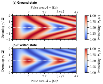
FIG. 3: Time evolution of the probability (density) $P_{j}$ with $j=g,e$ of finding an atom in the ground state (a)  and excited state (b)  during the laser pulse (plane waves) driving the ideal E1-M1 transitions. Initially the atom is assumed to be prepared in the ground state and the probability density is plotted as a function of relative detuning $\gamma$ in units of the Rabi frequency $|\Omega|=\Omega_{\text{eff}}|_{\gamma=0}$ at vanishing detuning. Increasing the relative detuning $\gamma$ increases the frequency of the Rabi oscillations, changes the amplitudes and thus shifts them to a different location in time at fixed relative detuning $\gamma$.

IV Finite Pulse-Time effects

Since electromagnetic fields have to satisfy Maxwell’s equations, the M1 couplings are suppressed by a factor of the inverse of the speed of light $c^{-1}$. Thus, they are much weaker than E1 transitions at typical laser intensities, and the two-photon Rabi frequency, Eq. (44), is quite small when comparing to the Rabi frequency associated with two E1 transitions. Accordingly, one needs pretty long or relatively intense laser pulses to achieve $\pi$- or $\pi/2$-pulses. That is why finite pulse-time effects become important for E1-M1 transitions. Since the transition between $\ket{g}$ and $\ket{e}$ is forbidden for single-photon transitions, however, we can still neglect spontaneous emission. In the idealized scenario of Sec. III we considered plane waves for the electromagnetic fields. However, a realistic laser beam has a position-dependent intensity, e.g. a Gaussian beam profile. At the same time, the Rabi frequencies from Eq. (40) depend on the amplitudes of the electric and magnetic fields, thereby also on the intensity. As a consequence, and due to the operator-valued nature of the atomic COM, the atoms might experience small, possibly state-dependent potentials due to the position dependency of the laser intensity while falling during a laser pulse. In particular, small perturbations in the already small magnetic field amplitude might have large effects. In order to find the effective time-evolution operator $\hat{U}_{\mathrm{eff}}$ for the atomic wave packet in weakly position-dependent pulses we replace

$$-\frac{\Omega^{*}_{B1}\Omega_{E0}}{2\Delta} \rightarrow-\frac{\Omega^{*}_{B1}(\hat{\boldsymbol{\mathbf{R}}})\Omega_{E0}(\hat{\boldsymbol{\mathbf{R}}})}{2\Delta}=:\Omega(\hat{\boldsymbol{\mathbf{R}}})\mathrm{e}^{\mathrm{i}\Phi(\hat{\boldsymbol{\mathbf{R}}})},$$ (58a)

$$\frac{|\Omega_{E0}|^{2}}{2\Delta} \rightarrow\frac{|\Omega_{E0}(\hat{\boldsymbol{\mathbf{R}}})|^{2}}{2\Delta}=:\omega_{\mathrm{AC},0}(\hat{\boldsymbol{\mathbf{R}}}),$$ (58b)

$$\frac{|\Omega_{B1}|^{2}}{2\Delta} \rightarrow\frac{|\Omega_{B1}(\hat{\boldsymbol{\mathbf{R}}})|^{2}}{2\Delta}=:\omega_{\mathrm{AC},1}(\hat{\boldsymbol{\mathbf{R}}}).$$ (58c)

Adding the atomic rest energy, the Hamiltonian describing the effective two-level atom via Eq. (39) becomes

$$\begin{split}\hat{H}=&\left(\frac{\hat{\boldsymbol{\mathbf{P}}}^{2}}{2M}+Mc^{2}\right)\!\mathds{1}+\hbar\left(\!\begin{array}[]{cc}\delta-\omega_{\mathrm{AC},1}(\hat{\boldsymbol{\mathbf{R}}})&\frac{\Omega(\hat{\boldsymbol{\mathbf{R}}})}{2}\mathrm{e}^{\mathrm{i}\Phi(\hat{\boldsymbol{\mathbf{R}}})}\\ \frac{\Omega(\hat{\boldsymbol{\mathbf{R}}})}{2}\mathrm{e}^{-\mathrm{i}\Phi(\hat{\boldsymbol{\mathbf{R}}})}&-\omega_{\mathrm{AC},0}(\hat{\boldsymbol{\mathbf{R}}})\end{array}\!\!\right)\!.\end{split}$$ (59)

The particular effects of the position dependency of the laser intensity can be separated by unitary transformations that cancel specific operator-valued terms in the Hamiltonian. First of all, let us cancel out the phase in the off-diagonal part in the Hamiltonian. This can be achieved by the unitary displacement transformation $\ket{\boldsymbol{\mathbf{\psi}}}\rightarrow\hat{U}_{1}^{\dagger}\ket{\boldsymbol{\mathbf{\psi}}}$, where

$$\hat{U}_{1}^{\dagger}=\left(\begin{array}[]{cc}\hat{\mathcal{D}}^{\dagger}&0\\ 0&1\end{array}\right)\;\;\text{and}\;\;\hat{\mathcal{D}}^{\dagger}=\exp\left(-\frac{\mathrm{i}}{\hbar}\left[\boldsymbol{\mathbf{\eta}}\hat{\boldsymbol{\mathbf{R}}}-\boldsymbol{\mathbf{\xi}}\hat{\boldsymbol{\mathbf{P}}}+\alpha\right]\right)$$ (62)

is the displacement operator. Assuming the wave packet to be, without loss of generality, initially centered around $\boldsymbol{\mathbf{R}}=0$, the phase in Eq. (58a) can thus be expanded around the origin in the COM position via

$$\Phi(\hat{\boldsymbol{\mathbf{R}}})=\Phi(0)+\hat{\boldsymbol{\mathbf{R}}}\cdot\nabla\Phi|_{\boldsymbol{\mathbf{R}}=0}+\varphi(\hat{\boldsymbol{\mathbf{R}}}),$$ (63)

where $\varphi(\hat{\boldsymbol{\mathbf{R}}})=\mathcal{O}(\hat{\boldsymbol{\mathbf{R}}}^{2})$, provided that the spatial extension of the wave packet is small enough compared to characteristic scales of the laser beam, e.g. the beam waist and the Rayleigh length for a Gaussian laser beam, and the laser pulse time is sufficiently small as the atom is falling, i.e. moving away from the initial position. This phase can then easily be eliminated by choosing the specific transformation parameters

$$\alpha=\hbar\Phi(0),\;\;\boldsymbol{\mathbf{\xi}}=0\;\;\text{and}\;\;\boldsymbol{\mathbf{\eta}}=\hbar\nabla\Phi|_{\boldsymbol{\mathbf{R}}=0}.$$ (64)

Thus, the unitary transformation, Eq. (62), corresponds to a small momentum kick

$$\hbar\boldsymbol{\mathbf{k}}=\hbar\nabla\Phi|_{\boldsymbol{\mathbf{R}}=0}.$$ (65)

Consequently, one can identify the recoil frequency $\omega_{k}$, the Doppler detuning $\nu(\hat{\boldsymbol{\mathbf{P}}})$ and the (position-dependent) mean AC Stark shift $\omega_{\mathrm{AC}}^{(+)}(\hat{\boldsymbol{\mathbf{R}}})$ (expanded around the origin) via the definitions

$$\begin{split}\omega_{k}&=\frac{\hbar\boldsymbol{\mathbf{k}}^{2}}{2M},\;\;\nu(\hat{\boldsymbol{\mathbf{P}}})=\frac{\boldsymbol{\mathbf{k}}\cdot\hat{\boldsymbol{\mathbf{P}}}}{M},\\ \text{and}\;\;\omega_{\mathrm{AC}}^{(+)}(\hat{\boldsymbol{\mathbf{R}}})&=\omega_{\mathrm{AC},0}(\hat{\boldsymbol{\mathbf{R}}})+\omega_{\mathrm{AC},1}(\hat{\boldsymbol{\mathbf{R}}})\\ &=\omega_{\mathrm{AC},0}^{(+)}+\hat{\boldsymbol{\mathbf{R}}}\cdot\nabla\omega_{\mathrm{AC}}^{(+)}|_{\boldsymbol{\mathbf{R}}=0}+\mathcal{S}(\hat{\boldsymbol{\mathbf{R}}}),\end{split}$$ (66)

where $\mathcal{S}(\hat{\boldsymbol{\mathbf{R}}})=\mathcal{O}(\hat{\boldsymbol{\mathbf{R}}}^{2})$ is the second (and higher) order part of the expansion of the mean AC Stark shift $\omega_{\mathrm{AC}}^{(+)}(\hat{\boldsymbol{\mathbf{R}}})$. The transformed Hamiltonian reads then

$$\hat{H}^{\prime}=\left(\begin{array}[]{cc}\hat{\bar{H}}+\frac{\Delta(\hat{\boldsymbol{\mathbf{R}}})}{2}-\hbar\mathcal{S}(\hat{\boldsymbol{\mathbf{R}}})&\hat{H}_{\mathrm{off}}\\ \hat{H}_{\mathrm{off}}^{\dagger}&\hat{\bar{H}}-\frac{\Delta(\hat{\boldsymbol{\mathbf{R}}})}{2}-\hbar\mathcal{S}(\hat{\boldsymbol{\mathbf{R}}})\end{array}\right),$$ (69)

where

$$\begin{split}\hat{\bar{H}}=&\frac{\hat{\boldsymbol{\mathbf{P}}}^{2}}{2M}+Mc^{2}+\frac{\hbar}{2}\Big{[}\hat{\nu}+\omega_{k}+\delta\\ &-\left(\omega_{\mathrm{AC},0}^{(+)}+\nabla\omega_{\mathrm{AC}}^{(+)}|_{\boldsymbol{\mathbf{R}}=0}\hat{\boldsymbol{\mathbf{R}}}\right)+\dot{\boldsymbol{\mathbf{k}}}\hat{\boldsymbol{\mathbf{R}}}+\dot{\Phi}(0)\Big{]}\end{split}$$ (70)

is the mean Hamiltonian,

$$\Delta(\hat{\boldsymbol{\mathbf{R}}})=\hbar\left(\hat{\nu}+\omega_{k}+\delta+\omega_{\mathrm{AC}}^{(-)}(\hat{\boldsymbol{\mathbf{R}}})+\dot{\boldsymbol{\mathbf{k}}}\hat{\boldsymbol{\mathbf{R}}}+\dot{\Phi}(0)\right)$$ (71)

is the detuning operator and

$$\hat{H}_{\mathrm{off}}=\hbar\,\frac{\Omega(\hat{\boldsymbol{\mathbf{R}}})}{2}\text{e}^{\mathrm{i}\varphi(\hat{\boldsymbol{\mathbf{R}}})}$$ (72)

is the off-diagonal part of the Hamiltonian; we denoted partial derivatives in time with a dot. Let us now transform into the interaction picture where we cancel out the dynamics of the mean Hamiltonian $\hat{\bar{H}}$, i.e. a unitary transformation with

$$\hat{\bar{U}}=\mathcal{T}\exp\left(-\frac{\mathrm{i}}{\hbar}\int_{0}^{t}\hat{\bar{H}}\;\mathrm{d}t^{\prime}\right),$$ (73)

where $\mathcal{T}$ is the time ordering operation. Since the Hamiltonian $\hat{H}^{\prime}$, Eq. (69), is a function of the COM momentum $\hat{\boldsymbol{\mathbf{P}}}$ and the COM position $\hat{\boldsymbol{\mathbf{R}}}$, the remaining operators of the transformed Hamiltonian are evaluated on the Heisenberg trajectories generated by $\hat{\bar{H}}$ via the Heisenberg equations of motion:

$$\frac{\mathrm{d}\hat{\boldsymbol{\mathbf{R}}}_{H}}{\mathrm{d}t}=\frac{\mathrm{i}}{\hbar}[\hat{\bar{H}},\hat{\boldsymbol{\mathbf{R}}}_{H}]\;\;\text{and}\;\;\frac{\mathrm{d}\hat{\boldsymbol{\mathbf{P}}}_{H}}{\mathrm{d}t}=\frac{\mathrm{i}}{\hbar}[\hat{\bar{H}},\hat{\boldsymbol{\mathbf{P}}}_{H}].$$ (74)

We denote the Heisenberg picture with a subscript $H$ and obtain the new Hamiltonian

$$\hat{H}^{\prime\prime}=\left(\begin{array}[]{cc}\frac{\Delta_{H}(\hat{\boldsymbol{\mathbf{R}}},t)}{2}-\hbar\mathcal{S}_{H}(\hat{\boldsymbol{\mathbf{R}}},t)&\hat{H}_{\mathrm{off},H}\\ \hat{H}^{\dagger}_{\mathrm{off},H}&-\frac{\Delta_{H}(\hat{\boldsymbol{\mathbf{R}}},t)}{2}-\hbar\mathcal{S}_{H}(\hat{\boldsymbol{\mathbf{R}}},t)\end{array}\right).$$ (77)

Note that terms of quadratic or higher order in COM position in the mean AC Stark shift $\omega_{\mathrm{AC}}^{(+)}(\hat{\boldsymbol{\mathbf{R}}})$ are encapsulated by $\mathcal{S}(\hat{\boldsymbol{\mathbf{R}}})$ so that the mean Hamiltonian $\hat{\bar{H}}$ of Eq. (70) is at most linear in atomic position $\hat{\boldsymbol{\mathbf{R}}}$. This will facilitate later on the back-transformation to the full unitary time evolution. From the calculations in Sec. III we know that in the idealized case without position dependency of the laser amplitude the internal dynamics of the atom is described by Rabi oscillations, see Eq. (57). These internal transitions can be canceled out of our Hamiltonian by the unitary transformation

$$\hat{U}_{\Omega}=\exp\left(-\mathrm{i}\frac{\Omega(0)}{2}t\hat{\sigma}_{x}\right),$$ (78)

with $\hat{\sigma}_{x}$ being the Pauli operator for the $x$-direction. After this final unitary transformation we are left with the Hamiltonian

$$\hat{H}_{3}(t)=\hat{H}_{0}(t)\,\mathds{1}+\sum_{j=\{x,y,z\}}\hat{H}_{j}(t)\hat{\sigma}_{j}$$

$$=-\hbar\mathcal{S}_{H}(\hat{\boldsymbol{\mathbf{R}}},t)\mathds{1}+\frac{\hbar}{2}\left[\Omega_{H}(\hat{\boldsymbol{\mathbf{R}}},t)\cos\left(\varphi_{H}(\hat{\boldsymbol{\mathbf{R}}},t)\right)-\Omega(0)\right]\hat{\sigma}_{x}$$

$$\quad+\frac{1}{2}\Big{[}\Delta_{H}(\hat{\boldsymbol{\mathbf{R}}},t)\sin\left(\Omega(0)t\right)$$

$$\left.\qquad-\hbar\Omega_{H}(\hat{\boldsymbol{\mathbf{R}}},t)\sin\left(\varphi_{H}(\hat{\boldsymbol{\mathbf{R}}},t)\right)\cos\left(\Omega(0)t\right)\right]\hat{\sigma}_{y}$$

$$\quad+\frac{1}{2}\Big{[}\Delta_{H}(\hat{\boldsymbol{\mathbf{R}}},t)\cos\left(\Omega(0)t\right)$$

$$\left.\qquad+\hbar\Omega_{H}(\hat{\boldsymbol{\mathbf{R}}},t)\sin\left(\varphi_{H}(\hat{\boldsymbol{\mathbf{R}}},t)\right)\sin\left(\Omega(0)t\right)\right]\hat{\sigma}_{z},$$ (79)

where $\hat{\sigma}_{y}$ and $\hat{\sigma}_{z}$ are the remaining Pauli operators. This Hamiltonian can be treated perturbatively to find the effective time evolution operator which allows us to provide the full evolution of the system after transforming back to the original picture.

IV.1 Example: Fundamental Gaussian Laser Beam

Let us continue with the simplest, most basic example for a position-dependent laser intensity profile: the Gaussian laser beam. Assuming the atom to be falling along the optical axis of the laser beam and being located near the beam waist $w_{0}$ during the laser pulse, i.e. the ratio $\|\hat{\varrho}/w_{0}\|$ and $\|\hat{Z}/z_{R}\|$ is small, where

$$\hat{\varrho}=\sqrt{\hat{X}^{2}+\hat{Y}^{2}}.$$ (80)

is the radial position operator ($z_{R}$ being the Rayleigh length), as well as cylindrical symmetry, we can expand the fundamental Gaussian Meschede (2015) electromagnetic field in cylindrical coordinates. Thus 

$$\boldsymbol{\mathbf{E}}_{0}(\hat{\boldsymbol{\mathbf{R}}}) =\frac{\boldsymbol{\mathbf{E}}_{0}w_{0}}{w(\hat{Z})}\exp\left[-\frac{\hat{\varrho}^{2}}{w^{2}(\hat{Z})}-\mathrm{i}k_{L}\frac{\hat{\varrho}^{2}}{2R(\hat{Z})}+\mathrm{i}\zeta(\hat{Z})\right],$$ (81a)

$$\boldsymbol{\mathbf{B}}_{1}(\hat{\boldsymbol{\mathbf{R}}}) =\frac{\boldsymbol{\mathbf{B}}_{1}w_{0}}{w(\hat{Z})}\exp\left[-\frac{\hat{\varrho}^{2}}{w^{2}(\hat{Z})}+\mathrm{i}k_{L}\frac{\hat{\varrho}^{2}}{2R(\hat{Z})}+\mathrm{i}\zeta(\hat{Z})\right],$$ (81b)

to second order in COM position, where (introducing the rescaled operator $\hat{\mathcal{Z}}=\hat{Z}/z_{R}$)

$$\begin{split}w^{-1}(\hat{Z})&=\left[w_{0}\sqrt{1+\hat{\mathcal{Z}}^{2}}\right]^{-1}=w_{0}^{-1}\left[1-\frac{1}{2}\hat{\mathcal{Z}}^{2}+\mathcal{O}\left(\hat{\mathcal{Z}}^{4}\right)\right]\end{split}$$ (82)

is the inverse of the spot size parameter,

$$\begin{split}R^{-1}(\hat{Z})&=\hat{Z}^{-1}\left[1+\hat{\mathcal{Z}}^{-2}\right]^{-1}=\frac{\hat{\mathcal{Z}}}{z_{R}}\left[1-\hat{\mathcal{Z}}^{2}+\mathcal{O}\left(\hat{\mathcal{Z}}^{4}\right)\right]\end{split}$$ (83)

the inverse of the radius of curvature and

$$\zeta(\hat{Z})=\arctan\hat{\mathcal{Z}}=\hat{\mathcal{Z}}+\mathcal{O}\left(\hat{\mathcal{Z}}^{3}\right)$$ (84)

is the Gouy phase. Introducing further the dimensionless operator $\hat{\rho}=\hat{\varrho}/w_{0}$ as well as using the definitions of the single-photon Rabi frequencies, Eq. (40), we can now determine the operators that are present in the final Hamiltonian, Eq. (79), via their definitions, Eqs. (58), (66) and (71), expanded to the second order in $\hat{\rho}$ and $\hat{\mathcal{Z}}$ in terms of the Heisenberg trajectories of $\hat{\bar{H}}$:

$$\Omega_{H}(\hat{\boldsymbol{\mathbf{R}}},t) \approx\Omega(0)\left[1-\hat{\mathcal{Z}}^{2}_{H}(t)-2\;\rho^{2}_{H}(t)\right],$$ (85a)

$$\varphi_{H}(\hat{\boldsymbol{\mathbf{R}}},t) \approx 0,$$ (85b)

$$\begin{split}\Delta_{H}(\hat{\boldsymbol{\mathbf{R}}},t)&\approx\hbar\left[\nu(\hat{\boldsymbol{\mathbf{P}}}_{H}(t))+\omega_{k}+\delta\right.\\ &\left.\quad\quad+\left(1-\hat{\mathcal{Z}}^{2}_{H}(t)-2\;\rho^{2}_{H}(t)\right)\omega_{\mathrm{AC}}^{(-)}(0)\right],\end{split}$$ (85c)

$$\mathcal{S}_{H}(\hat{\boldsymbol{\mathbf{R}}},t) \approx-\frac{1}{2}\omega_{\mathrm{AC}}^{(+)}(0)\left(\hat{\mathcal{Z}}^{2}_{H}(t)+2\;\rho^{2}_{H}(t)\right),$$ (85d)

where we used $\Omega(0)=-\Omega_{E}\Omega_{B}^{*}/(2\Delta)$ and $\omega_{\mathrm{AC}}^{(\pm)}(0)=(|\Omega_{E}|^{2}\pm|\Omega_{B}|^{2})/(2\Delta)$. Note, that we have defined the position-independent Rabi frequencies $\Omega_{E}$ and $\Omega_{B}$ in total analogy to Eq. (40). Recalling Eqs. (40), (58) and (65), the effective kick due to the Gaussian beam shape is then given by

$$\hbar\boldsymbol{\mathbf{k}}=\hbar\nabla\Phi|_{\boldsymbol{\mathbf{R}}=0}=\frac{2\hbar}{z_{R}}\boldsymbol{\mathbf{e}}_{Z}.$$ (86)

In App. A we show that for this setup the Hamiltonian $\hat{H}_{3}$ of Eq. (79) is (quasi-)commuting at different times within the time scale we are interested in. Calculating the time-evolution operator,

$$\hat{U}_{3}(t)=\mathcal{T}\exp\left(-\frac{\mathrm{i}}{\hbar}\int_{0}^{t}\hat{H}_{3}(t^{\prime})\;\mathrm{d}t^{\prime}\right),$$ (87)

the time-ordering operation can thus be ignored. Instead, we can directly compute the integral in the exponent approximating all radial components up to the order $\mathcal{O}(\hat{\rho}^{2})$ and all $Z$-components to the order $\mathcal{O}(\hat{\mathcal{Z}}^{2})$, i.e. the wave packet is sufficiently localized with respect to $w_{0}$ in radial and $z_{R}$ in $Z$-direction. Introducing further the dimensionless time $\tau=\Omega(0)t$, we obtain the time-evolution operator

$$\hat{U}_{3}(\tau)=\exp\!\Bigg{\{}\! \frac{-\mathrm{i}\,\tau}{2}\frac{\omega_{\mathrm{AC}}^{(+)}(0)}{\Omega(0)}\left(\hat{\mathcal{Z}}^{2}+2\,\hat{\rho}^{2}\right)\!\mathds{1}+\frac{\mathrm{i}\,\tau}{2}\!\left(\hat{\mathcal{Z}}^{2}+2\,\hat{\rho}^{2}\right)\hat{\sigma}_{x}$$

$$-\frac{\mathrm{i}}{2\Omega(0)}\left[\nu(\hat{\boldsymbol{\mathbf{P}}})-\omega_{\mathrm{AC}}^{(-)}(0)\left(\hat{\mathcal{Z}}^{2}+2\,\hat{\rho}^{2}\right)\right]$$

$$\quad\times\left[\left(1-\cos(\tau)\right)\hat{\sigma}_{y}+\sin(\tau)\,\hat{\sigma}_{z}\right]\Bigg{\}}.$$ (88)

Furthermore, we chose the overall detuning $\delta=-\omega_{k}-\omega_{\mathrm{AC}}^{(-)}(0)$ to compensate the differential AC Stark shift $\omega_{\mathrm{AC}}^{(-)}(0)$ and the recoil frequency $\omega_{k}$. Finally, we assume that the atoms are near the origin, i.e. $\|\hat{\mathcal{Z}}^{2}\|_{\ket{\psi}}\ll 1$ and $\|\hat{\rho}^{2}\|_{\ket{\psi}}\ll 1$ for our wave packets. Thus, all terms of the order $\mathcal{O}(\hat{\mathcal{Z}}^{2})$ and $\mathcal{O}(\hat{\rho}^{2})$ can be neglected and we obtain the time evolution operator

$$\begin{split}&\hat{U}_{3}(\tau)=\exp\left\{-\frac{\mathrm{i}\nu(\hat{\boldsymbol{\mathbf{P}}})}{2\Omega(0)}\left[\left(1-\cos(\tau)\right)\hat{\sigma}_{y}+\sin(\tau)\hat{\sigma}_{z}\right]\right\}\\ &=\cos\left[\frac{\nu(\hat{\boldsymbol{\mathbf{P}}})}{\Omega(0)}\sin\left(\frac{\tau}{2}\right)\right]\mathds{1}+\mathrm{i}\sin\left[\frac{\nu(\hat{\boldsymbol{\mathbf{P}}})}{\Omega(0)}\sin\left(\frac{\tau}{2}\right)\right]\\ &\quad\times\left(\sin\left(\frac{\tau}{2}\right)\hat{\sigma}_{y}+\cos\left(\frac{\tau}{2}\right)\hat{\sigma}_{z}\right).\end{split}$$ (89)

To consider now all finite pulse-time effects for a Gaussian laser beam, the unitary transformations done in this section as well as the displacement transformation, Eq. (24), have to be reversed. Doing this subsequently and using $\hat{\bar{U}}^{\dagger}(0)=\hat{U}_{\Omega}^{\dagger}(0)=\mathds{1}$, we end up with

$$\hat{U}(\tau)=\hat{D}(\tau)\hat{U}_{1}\hat{\bar{U}}(\tau)\hat{U}_{\Omega}(\tau)\hat{U}_{3}(\tau)\hat{U}_{1}^{\dagger}\hat{D}^{\dagger}(0)$$ (90)

being the total time evolution in the initial picture, cf. Eq. (39). Inserting $\tau_{\pi}=\pi$ ($\tau_{\pi/2}=\pi/2$) for the duration of a $\pi$-pulse ($\pi/2$-pulse) we obtain the generalized $\pi$-pulse and $\pi/2$-pulse operators:

$$\hat{U}_{\pi}=\left(\begin{array}[]{cc}\hat{U}_{\pi,ee}&\hat{U}_{\pi,ge}\\ \hat{U}_{\pi,eg}&\hat{U}_{\pi,gg}\end{array}\right)\;\;\text{and}\;\;\hat{U}_{\frac{\pi}{2}}=\left(\begin{array}[]{cc}\hat{U}_{\frac{\pi}{2},ee}&\hat{U}_{\frac{\pi}{2},ge}\\ \hat{U}_{\frac{\pi}{2},eg}&\hat{U}_{\frac{\pi}{2},gg}\end{array}\right)$$ (95)

with

$$\hat{U}_{\pi,ee} =\mathrm{i}\hat{D}(\tau)\hat{\mathcal{D}}\hat{\bar{U}}\left(\pi\right)\sin\left(\frac{\nu(\hat{\boldsymbol{\mathbf{P}}})}{\Omega(0)}\right)\hat{\mathcal{D}}^{\dagger}\hat{D}^{\dagger}(0),$$ (96a)

$$\hat{U}_{\pi,ge} =-\mathrm{i}\hat{D}(\tau)\hat{\mathcal{D}}\hat{\bar{U}}\left(\pi\right)\cos\left(\frac{\nu(\hat{\boldsymbol{\mathbf{P}}})}{\Omega(0)}\right)\hat{D}^{\dagger}(0),$$ (96b)

$$\hat{U}_{\pi,eg} =-\mathrm{i}\hat{D}(\tau)\hat{\bar{U}}\left(\pi\right)\cos\left(\frac{\nu(\hat{\boldsymbol{\mathbf{P}}})}{\Omega(0)}\right)\hat{\mathcal{D}}^{\dagger}\hat{D}^{\dagger}(0),$$ (96c)

$$\hat{U}_{\pi,gg} =-\mathrm{i}\hat{D}(\tau)\hat{\bar{U}}\left(\pi\right)\sin\left(\frac{\nu(\hat{\boldsymbol{\mathbf{P}}})}{\Omega(0)}\right)\hat{D}^{\dagger}(0),$$ (96d)

and

$$\begin{split}\hat{U}_{\frac{\pi}{2},ee}&=\frac{1}{\sqrt{2}}\hat{D}(\tau)\hat{\mathcal{D}}\hat{\bar{U}}\left(\frac{\pi}{2}\right)\bigg{[}\cos\left(\frac{\nu(\hat{\boldsymbol{\mathbf{P}}})}{\sqrt{2}\Omega(0)}\right)\\ &\quad+\sqrt{2}\text{i}\sin\left(\frac{\nu(\hat{\boldsymbol{\mathbf{P}}})}{\sqrt{2}\Omega(0)}\right)\bigg{]}\hat{\mathcal{D}}^{\dagger}\hat{D}^{\dagger}(0),\end{split}$$ (97a)

$$\hat{U}_{\frac{\pi}{2},ge} =-\frac{\text{i}\hat{D}(\tau)\hat{\mathcal{D}}\hat{\bar{U}}\left(\frac{\pi}{2}\right)\cos\left(\frac{\nu(\hat{\boldsymbol{\mathbf{P}}})}{\sqrt{2}\Omega(0)}\right)\hat{D}^{\dagger}(0)}{\sqrt{2}},$$ (97b)

$$\hat{U}_{\frac{\pi}{2},eg} =-\frac{\text{i}\hat{D}(\tau)\hat{\bar{U}}\left(\frac{\pi}{2}\right)\cos\left(\frac{\nu(\hat{\boldsymbol{\mathbf{P}}})}{\sqrt{2}\Omega(0)}\right)\hat{\mathcal{D}}^{\dagger}\hat{D}^{\dagger}(0)}{\sqrt{2}},$$ (97c)

$$\begin{split}\hat{U}_{\frac{\pi}{2},gg}&=\frac{1}{\sqrt{2}}\hat{D}(\tau)\hat{\bar{U}}\left(\frac{\pi}{2}\right)\bigg{[}\cos\left(\frac{\nu(\hat{\boldsymbol{\mathbf{P}}})}{\sqrt{2}\Omega(0)}\right)\\ &\quad-\sqrt{2}\text{i}\sin\left(\frac{\nu(\hat{\boldsymbol{\mathbf{P}}})}{\sqrt{2}\Omega(0)}\right)\bigg{]}\hat{D}^{\dagger}(0).\end{split}$$ (97d)

Recall the displacement operators $\hat{D}(t)$, Eq. (24), and $\hat{\mathcal{D}}$, Eq. (62), and the time evolution operator $\hat{\bar{U}}$ corresponding to the mean Hamiltonian $\hat{\bar{H}}$, Eq. (70). In the limit $z_{R}\to\infty$ (accordingly also $w_{0}\to\infty$ due to the relation $z_{R}=\pi w_{0}^{2}/\lambda$, where $\lambda$ is the wavelength of the laser beam, and $\boldsymbol{\mathbf{k}}=2\boldsymbol{\mathbf{e}}_{Z}/z_{R}\to 0$) they reduce to the well-known ideal $\pi$ and $\frac{\pi}{2}$-pulse operators, respectively,

$$\hat{U}_{\pi,\mathrm{ideal}} =\left(\begin{array}[]{cc}0&-\mathrm{i}\\ -\mathrm{i}&0\end{array}\right),\quad\hat{U}_{\frac{\pi}{2},\mathrm{ideal}}=\frac{1}{\sqrt{2}}\left(\begin{array}[]{cc}1&-\mathrm{i}\\ -\mathrm{i}&1\end{array}\right),$$ (102)

i.e. the plane wave solution of the previous section where the COM momentum $\hat{\boldsymbol{\mathbf{P}}}$ has no effect on the E1-M1 transitions.

IV.1.1 Discussion of the Generalized $\pi$ and $\pi/2$-Pulse Operators

Comparing the generalized $\pi$ and $\pi/2$-pulse operators, Eqs. (96) and  (97), with the ideal operators, Eq. (102), one can observe some additional effects due to the finite pulse time and the position dependency of the intensity of a Gaussian laser beam:

Additional momentum kicks

The displacement operators $\hat{\mathcal{D}}$ and $\hat{\mathcal{D}}^{\dagger}$ correspond to a transfer of momentum $\pm\hbar\boldsymbol{\mathbf{k}}=\pm\hbar\frac{\boldsymbol{\mathbf{e}}_{Z}}{2z_{R}}$, i.e. the transitions from ground to excited state and vice versa are accompanied by small additional momentum kicks. Note, that although there are displacement operators present in the terms $\hat{U}_{\pi,ee}$ and $\hat{U}_{\frac{\pi}{2},ee}$, i.e. the atoms remaining in the excited state during the laser pulse, the momentum of the atom is identical before and after the pulse. There is only a momentum shift occuring during the interaction with the laser.

Action of $\hat{\bar{U}}(\tau)$

The time-evolution operator

$$\hat{\bar{U}}(\tau)=\exp\!\left[\frac{-\mathrm{i}\tau}{\hbar\Omega(0)}\left(\frac{\hat{\boldsymbol{\mathbf{P}}}^{2}}{2M}+\frac{\hbar\nu(\hat{\boldsymbol{\mathbf{P}}})}{2}+Mc^{2}-\frac{\hbar|\Omega_{E}|^{2}}{2\Delta}\right)\!\right]$$ (103)

associated with the mean Hamiltonian, Eq. (70), corresponds to a displacement $-\hbar\tau/(Mz_{R}\Omega(0))$ in $Z$-direction (recall Eqs. (66) and (86)) and a laser phase. Recall that we chose the overall detuning $\delta=-\omega_{k}-\omega_{\mathrm{AC}}^{(-)}(0)$ so that the recoil frequency $\omega_{k}$ and the part of the mean AC Stark shift $\omega_{\mathrm{AC}}^{(+)}(0)$ corresponding to the M1 transition in zeroth order, i.e. $|\Omega_{B}|^{2}/(2\Delta)$, is compensated in the mean Hamiltonian. Furthermore, the first order of the mean AC Stark shift vanishes for the $\text{TEM}_{00}$ laser mode.

Additional branches

The $\pi$ and $\pi/2$-pulses further contain operators of the form $\sin(\xi\hat{P}_{z}/\hbar)$ and $\cos(\xi\hat{P}_{z}/\hbar)$, i.e. a splitting of the branches in opposite directions. Moreover, we see that the $\pi$ and $\pi/2$-pulse operators do not transform all the atoms to the appropriate internal state (in contrast to the ideal case). Both, the $\pi$- and $\pi/2$-pulses lead therefore to a splitting into four branches.

However, the order of magnitude of the displacements in space during the pulse time, i.e. $\mathcal{O}(\hbar/(z_{R}M\Omega(0)))$, is much smaller than the displacement due to the momentum kick which is of the order $\mathcal{O}(\hbar T/(Mz_{R}))$, since $\Omega(0)T\gg 1$ (cf. Table 1 in App. A), and where $T$ is a characteristic time of the interferometer sequence, e.g. $T=T_{4}-T_{2}$ in Fig. 4 or $T=T_{3}-T_{2}$ in Fig. 5. Therefore we will neglect branch splitting from now on and continue with the $\pi$- and $\pi/2$-pulse operators given by

$$\hat{U}_{\pi} =-\text{i}\hat{D}(\tau)\left(\begin{array}[]{cc}0&\hat{\mathcal{D}}\hat{\bar{U}}^{\prime}\left(\pi\right)\\ \hat{\bar{U}}^{\prime}\left(\pi\right)\hat{\mathcal{D}}^{\dagger}&0\end{array}\right)\hat{D}^{\dagger}(0),$$ (104c)

$$\hat{U}_{\frac{\pi}{2}} =\frac{1}{\sqrt{2}}\hat{D}(\tau)\left(\begin{array}[]{cc}\hat{\bar{U}}^{\prime}\left(\frac{\pi}{2}\right)&-\mathrm{i}\hat{\mathcal{D}}\hat{\bar{U}}^{\prime}\left(\frac{\pi}{2}\right)\\ -\mathrm{i}\hat{\bar{U}}^{\prime}\left(\frac{\pi}{2}\right)\hat{\mathcal{D}}^{\dagger}&\hat{\bar{U}}^{\prime}\left(\frac{\pi}{2}\right)\end{array}\right)\hat{D}^{\dagger}(0),$$ (104f)

where

$$\hat{\bar{U}}^{\prime}(\tau)=\exp\left[-\frac{\mathrm{i}\tau}{\hbar\Omega(0)}\left(Mc^{2}+\frac{\hat{\boldsymbol{\mathbf{P}}}^{2}}{2M}-\hbar\frac{|\Omega_{E}|^{2}}{2\Delta}\right)\right]$$ (105)

is the time-evolution due to the mean Hamiltonian Eq. (70) without the term inducing spatial translations since

$$\left\|\frac{\hat{P}_{z}}{Mz_{R}\Omega(0)}\right\|\ll 1.$$ (106)

V Effects on the interferometer phase from additional momentum kicks

In this section we investigate the main finite pulse-time effects for E1-M1 transitions, namely the falling of the atom during the laser pulse and the additional momentum kicks, for UGR and UFF tests using the interferometer schemes (A) Roura (2020) and (B) Ufrecht et al. (2020) (recall Sec. II). We assume ideal momentum kick operators

$$\hat{\mathcal{D}}_{p}=\frac{1}{\sqrt{2}}\text{e}^{\text{i}k_{p}\hat{Z}}$$ (107)

for the (magic) Bragg pulses, i.e. momentum transfer pulses that do not change the internal state, as well as for the $\pi$ and $\pi/2$-pulses, see Eq. (104) in Sec. IV. The evolution of the atom in the gravitational field from time $T_{k}$ to $T_{i}$ in between laser pulses in its ground/excited state can be described via Loriani et al. (2019); Roura (2020); Ufrecht et al. (2020)

$$\hat{U}(T_{i},T_{k})=\sum_{\mathclap{n=g,e}}\text{e}^{-\frac{\mathrm{i}}{\hbar}\hat{H}^{\text{(ME)}}_{n}\left(T_{i}-T_{k}\right)}\outerproduct{n}{n}=\sum_{\mathclap{n=g,e}}\hat{U}_{n}(T_{i},T_{k})\outerproduct{n}{n}.$$ (108)

Since this Hamiltonian is diagonal in the internal states, calculating the evolution during the free fall of the atoms is particularly easy, and reduces to finding the time evolution operators $\hat{U}_{n}(T_{i},T_{k})$ corresponding to the Hamiltonian $\hat{H}_{n}^{(\text{ME})}=H(\hat{\boldsymbol{\mathbf{R}}},\hat{\boldsymbol{\mathbf{P}}};M_{n})$. On the other hand, one could also use the mass defect representation of the Hamiltonian $\hat{H}^{(\text{MD})}$ and calculate the evolution via $\hat{U}(T_{i},T_{k})=\text{e}^{-\frac{\text{i}}{\hbar}\hat{H}^{(\text{MD})}(T_{i}-T_{k})}$ which is however much more complicated than rewriting the previous result.

We assume further that the initial COM state $\ket{\psi_{0}}$ of the atom corresponds to a $L^{2}$-normalized Gaussian wave packet

$$\psi_{0}(\boldsymbol{\mathbf{P}})=\frac{\exp\left({-\frac{1}{4}(\boldsymbol{\mathbf{P}}-\boldsymbol{\mathbf{P}}_{0})^{T}\boldsymbol{\mathbf{\sigma}}^{-1}(\boldsymbol{\mathbf{P}}-\boldsymbol{\mathbf{P}}_{0})}\right)}{(2\pi)^{3/4}\operatorname{det}^{1/4}\boldsymbol{\mathbf{\sigma}}},$$ (109)

with covariance matrix $\boldsymbol{\mathbf{\sigma}}=\text{diag}((\Delta p_{x})^{2},(\Delta p_{y})^{2},(\Delta p_{z})^{2})$ and mean momentum $\boldsymbol{\mathbf{P}}_{0}$. We can thus describe the full initial atomic state by a product state

$$\ket{\Psi_{0}}=\ket{\phi_{\mathrm{i}}}\otimes\ket{\psi_{0}},$$ (110)

where $\ket{\phi_{\mathrm{i}}}$ is the initial internal state of the atom. Using the exit port projection operator

$$\hat{\Pi}_{\text{exit}}=\outerproduct{\phi_{\mathrm{f}}}{\phi_{\mathrm{f}}}\otimes\hat{\Pi}_{\text{exit}}^{\text{(COM)}},$$ (111)

the measured intensity in the respective exit port (excited or ground state) is then described by

$$I_{\phi_{\mathrm{f}}}=\matrixelement{\psi_{0}}{\left[\matrixelement{\phi_{\mathrm{f}}}{\hat{\Pi}_{\text{exit}}^{(\text{COM})}\hat{U}_{\mathrm{tot}}}{\phi_{\mathrm{i}}}\right]^{\dagger}\matrixelement{\phi_{\mathrm{f}}}{\hat{\Pi}_{\text{exit}}^{(\text{COM})}\hat{U}_{\mathrm{tot}}}{\phi_{\mathrm{i}}}}{\psi_{0}},$$ (112)

where

$$\matrixelement{\phi_{\mathrm{f}}}{\hat{\Pi}_{\text{exit}}^{(\text{COM})}\hat{U}_{\mathrm{tot}}}{\phi_{\mathrm{i}}}=\hat{U}_{l,\phi_{\mathrm{i}}\phi_{\mathrm{f}}}+\hat{U}_{u,\phi_{\mathrm{i}}\phi_{\mathrm{f}}}$$ (113)

is the sum of the evolution operators along the lower and the upper branches leading to the exit port of the interferometer characterized by the internal state $\ket{\phi_{\mathrm{f}}}$ and the projector $\hat{\Pi}_{\text{exit}}^{(\text{COM})}$ on the COM degrees of freedom corresponding to the exit port.

V.1 UGR Tests Using Superpositions of Internal States

In the interferometer scheme (A) Roura (2020) the atoms entering the interferometer in the ground state are divided into two branches, and in the middle segment a Doppler-free $\pi/2$-pulse is applied simultaneously on both branches to get a 50:50 superposition of excited and ground state atoms, i.e. the initialization of an atomic clock.

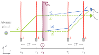
FIG. 4: Interferometer scheme (A) of Roura Roura (2020) in the freely falling frame modified by finite pulse-time effects during the E1-M1 $\frac{\pi}{2}$-pulse. Initially the atomic wave packet is prepared in the ground state $\ket{g}$ (green) before being diffracted by (magic) Bragg pulses at times $T_{0},\leavevmode\nobreak\ T_{1},\leavevmode\nobreak\ T_{3}$ and $T_{4}$. During each of the Bragg diffraction light pulses (red) the momentum of the atoms changes only for parts of the atoms. At all but the first Bragg pulse some of the atoms are not diffracted along the branches of the interferometer and hence do not propagate into the exit port. We do not illustrate these additional paths for clarity. At time $T_{2}$ an E1-M1 pulse of duration $t_{\frac{\pi}{2}}$ at time $T_{2}$ (violet pulse and shading) initialized a delocalized supersposition of ground (green) and excited state (blue) on both branches. Additional momentum kicks $\hbar\boldsymbol{\mathbf{k}}$ originating from the optical potentials acting during the transition at time $T_{2}$ lead to an additional spatial delocalization of the clock states along the interferometer branches (illustrated unrealistically large). At the end of the interferometer this kick-induced delocalization along the branches between the clock states leads to slightly displaced detection locations for the ground (green) and excited state (blue) atoms.

However, considering finite pulse-time effects, the E1-M1 transitions are not Doppler-free anymore. The modified trajectories of this interferometer are shown in Fig. 4. Nevertheless, we can still measure the intensity in the ground state and the excited state exit ports. Describing the evolution along the lower and upper trajectories, respectively, by

$$\hat{U}_{l,gg} =\frac{1}{2}\hat{\mathcal{D}}_{p}^{\dagger}\hat{U}_{g}(T_{4},T_{3})\hat{\mathcal{D}}_{p}\hat{U}_{g}(T_{3},T_{2}+t_{\frac{\pi}{2}})\hat{U}_{\frac{\pi}{2},gg}\hat{U}_{g}(T_{2},T_{0}),$$ (114a)

$$\hat{U}_{u,gg} =\frac{1}{2}\hat{U}_{g}(T_{4},T_{2}+t_{\frac{\pi}{2}})\hat{U}_{\frac{\pi}{2},gg}\hat{U}_{g}(T_{2},T_{1})\hat{\mathcal{D}}_{p}^{\dagger}\hat{U}_{g}(T_{1},T_{0})\hat{\mathcal{D}}_{p},$$ (114b)

which leads to

$$\hat{U}_{l,gg}^{\dagger}\hat{U}_{l,gg}=\hat{U}_{u,gg}^{\dagger}\hat{U}_{u,gg}=\frac{1}{32},$$ (115)

the intensity in the ground state exit port is given by

$$I_{g} =\frac{1}{16}+\matrixelement{\psi_{0}}{\left(\hat{U}_{u,gg}^{\dagger}\hat{U}_{l,gg}+\mathrm{h.c.}\right)}{\psi_{0}}$$

$$=\frac{1}{32}\left[2+\left(\mathcal{V}_{g}\mathrm{e}^{\mathrm{i}\Delta\phi_{g}}+\mathrm{c.c.}\right)\right],$$ (116)

where we defined the visibility $\mathcal{V}_{g}$ and the phase difference $\Delta\phi_{g}$ in the ground state exit port. Analogously we obtain for the excited state exit port the lower and upper branch evolution operators,

$$\hat{U}_{l,ge} =\frac{1}{2}\hat{\mathcal{D}}_{p}^{\dagger}\hat{U}_{e}(T_{4},T_{3})\hat{\mathcal{D}}_{p}\hat{U}_{e}(T_{3},T_{2}+t_{\frac{\pi}{2}})\hat{U}_{\frac{\pi}{2},ge}\hat{U}_{g}(T_{2},T_{0}),$$ (117a)

$$\hat{U}_{u,ge} =\frac{1}{2}\hat{U}_{e}(T_{4},T_{2}+t_{\frac{\pi}{2}})\hat{U}_{\frac{\pi}{2},ge}\hat{U}_{g}(T_{2},T_{1})\hat{\mathcal{D}}_{p}^{\dagger}\hat{U}_{g}(T_{1},T_{0})\hat{\mathcal{D}}_{p},$$ (117b)

leading to the intensity in the excited state exit port

$$I_{e} =\frac{1}{16}+\matrixelement{\psi_{0}}{\left(\hat{U}_{u,ge}^{\dagger}\hat{U}_{l,ge}+\mathrm{h.c.}\right)}{\psi_{0}}$$

$$=\frac{1}{32}\left[2+\left(\mathcal{V}_{e}\mathrm{e}^{\mathrm{i}\Delta\phi_{e}}+\mathrm{h.c.}\right)\right]$$ (118)

with the visibility $\mathcal{V}_{e}$ and the phase difference $\Delta\phi_{e}$ in the excited state exit port. Inserting the Gaussian wave packet from Eq. (109) we can calculate the visibility and the phase

$$\mathcal{V}_{g} =1,\quad\Delta\phi_{g}=\frac{1}{2}gk_{p}\delta T\left(T_{4}+T_{3}-\delta T\right)+\frac{\epsilon}{2}gk_{p}t_{\frac{\pi}{2}}\delta T$$ (119)

in the ground state exit port and

$$\begin{split}\mathcal{V}_{e}&=\exp\left(-\frac{k_{p}^{2}\epsilon^{2}\Delta p_{z}^{2}\delta T^{2}}{2M^{2}}\right)=1+\mathcal{O}\left(\epsilon^{2}\right),\\ \Delta\phi_{e}&=\frac{1}{2}gk_{p}\delta T\left(T_{4}+T_{3}-\delta T\right)-\frac{\hbar kk_{p}\delta T}{M}\\ &\quad\quad+\epsilon\left(\frac{\hbar(k+k_{p})k_{p}\delta T}{2M}-\frac{1}{2}gk_{p}\delta T(t_{\frac{\pi}{2}}+2T_{2})\right)\end{split}$$ (120)

for the excited state exit port, and where we expanded everything up to the first order in $\epsilon=\Delta M/M$. Accordingly, the visibility is one to our order in the approximations for both channels. The differential phase is then given by

$$\begin{split}\Delta\phi_{-}=&\Delta\phi_{g}-\Delta\phi_{e}\\ =&\frac{\hbar kk_{p}\delta T}{M}-\epsilon\left(\frac{\hbar(k+k_{p})k_{p}\delta T}{2M}-gk_{p}\delta T(t_{\frac{\pi}{2}}+T_{2})\right),\end{split}$$ (121)

where we still observe finite pulse-time effects, i.e. the terms containing the additional momentum kick $\hbar k$ and the $\pi/2$ pulse time $t_{\frac{\pi}{2}}$. However, the double differential phase, i.e. the difference of the differential phase, Eq. (121), with different initialization times of the atomic clock $T_{2}$, is given by

$$\Delta\phi_{-}(T_{2})-\Delta\phi_{-}(T_{2}+\tau)=-\epsilon gk_{p}\delta T\tau.$$ (122)

Therefore, the finite pulse-time effects cancel each other between different runs of the experiment to the leading order in the expansion parameters.

V.2 UGR and UFF Tests Without Superposition

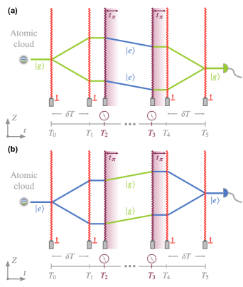
FIG. 5: Interferometer scheme (B) of Ufrecht et al. Ufrecht et al. (2020) in the freely falling frame for different initial states of the atoms. Panel (a) showcases the interferometer sequence with the atoms initially and at detection in the ground state $\ket{g}$. Panel (b) shows the corresponding sequence with atoms initially and at detection in the excited state $\ket{e}$. The E1-M1 $\pi$-pulses of duration $t_{\pi}$ are indicated by the violet lasers and subsequent violet shading after the beginning of the pulses at times $T_{2}$ and $T_{3}$. We exaggerated the separation between the momentum-kick pulses and the E1-M1 pulses as well as the effect of the modified momentum kicks $\pm\hbar\boldsymbol{\mathbf{k}}$ due to the additional optical potentials acting during the finite-duration E1-M1 transitions starting at times $T_{2}$ and $T_{3}$ for better visualization.

The interferometer scheme (B) Ufrecht et al. (2020) does not require superpositions of different internal states but a change of the internal state in the middle segment, i.e. a recoilless $\pi$-pulse. Again, we need two runs of the experiment: one with the initial ground state and one with the initial excited state. We found in Sec. IV.1 that the E1-M1 transitions are not perfectly recoilless for realistic beam shapes and finite pulse times. Likewise, the interferometer scheme in this section is modified by additional momentum kicks during the $\pi$-pulses, see Fig. 5.

We can calculate the final intensity analogously to the previous section and set $T_{3}-T_{2}=T_{4}-T_{1}=T$, so that we obtain the visibilities and phases

$$\mathcal{V}_{g} =1,\quad\Delta\phi_{g}=2gk_{p}\delta T\big{(}\delta T+T+\epsilon T\big{)}$$ (123)

for an initial ground state and

$$\mathcal{V}_{e} =1,\quad\Delta\phi_{e}=2gk_{p}\delta T\big{(}\delta T+T-\epsilon T\big{)}$$ (124)

for an initial excited state. For this interferometer scheme we find that the final pulse-time effects cancel each other already in the non-differential phase due to the symmetry of the interferometer. The results Ufrecht et al. (2020) can thus be reproduced immediately, i.e. the differential signals read

$$\Delta\phi_{+} =\Delta\phi_{g}+\Delta\phi_{e}=4gk_{p}(\delta T+T)\delta T,$$ (125a)

$$\Delta\phi_{-} =\Delta\phi_{g}-\Delta\phi_{e}=4\epsilon gk_{p}T\delta T,$$ (125b)

separating the effects of UFF and UGR.

VI Conclusion

Very-large baseline atom interferometry is built upon exploiting the beneficial scaling of the interferometer signal in terms of the enclosed space-time area. However, due to the resulting long free-fall and interaction times, imperfections and perturbations act over much longer timescales and even small, accumulated effects can lead to a loss of visibility in the interference pattern in such devices. In case of (local) magnetic and gravitational field gradients Wodey et al. (2020); Lezeik et al. (2023) these effects have to be studied in detail for upcoming large baseline setups in addition to the already available results for e.g. gravity gradients or rotations Roura, Zeller, and Schleich (2014); Lan et al. (2012); Dickerson et al. (2013); Roura (2017); Overstreet et al. (2018); Ufrecht (2021). In this spirit, our manuscript may be regarded as an extension of such studies to the case of E1-M1 transitions in quantum clock interferometry, performed under realistic conditions arising in large baseline atomic fountains.

Following the recent proposals of Roura Roura (2020) and Ufrecht et al. Ufrecht et al. (2020) for LPAI schemes that are sensitive to UGR and UFF tests, we have investigated recoil-less clock transitions mediated by E1-M1 processes. For this purpose, we took into account the fully quantized atomic degrees of freedom, including the quantized – and possibly delocalizing – COM motion as well as the intern-extern coupling/mass defect. As a simple starting point we considered electromagnetic plane waves in a $\sigma^{+}$- $\sigma^{-}$ polarization scheme such that the atom absorbs two counter-propagating field excitations. After an adiabatic elimination procedure we found that the internal atomic dynamics yield standard Rabi oscillations, where the COM dependency drops out due to the fields having a constant intensity in space.

However, since the M1 transitions are much weaker than E1 transitions in typical atoms one needs quite large laser intensities and still long pulse times in an interferometer scheme containing E1-M1 transitions. Accordingly, finite pulse-time effects need to be included for a precise modeling. Further, we also took into account that a realistic laser beam has a spatially dependent intensity, i.e. the Rabi frequencies become position dependent. Here we considered the case of an atom falling through a general laser beam with arbitrary spatial coupling and finite pulse times, and provided an expression for the dynamics of such an atom. In the exemplary case of a Gaussian laser beam, we derived $\pi$ and $\pi/2$-pulse operators that generalize the standard expressions. In particular, our results show additional momentum kicks $\pm 2\hbar/z_{R}\boldsymbol{\mathbf{e}}_{Z}$ to first order in the inverse Rayleigh length $z_{R}^{-1}$ and a splitting of the branches to second order in $z_{R}^{-1}$. As one would expect, these expressions reduce then to the idealized operators when we neglect the laser profile and assume a strictly localized atomic COM wave function.

It is important to emphasize that the laser inhomogeneities result in corrections to the idealized plane-wave model already for very localized atomic wave packets. In the case of atomic clouds that are suffering from strong dispersion, e.g. for long interferometer times or strong atom-atom interactions, the assumption of large scale separation between atomic and laser extension no longer holds, and the efficiency of optical pulses is expected to be reduced even further; cf. for instance the efficiency of a Bragg beam splitter with two E1 transitions. Neumann, Gebbe, and Walser (2021)

Finally, we returned to the initial question of the manuscript and applied our results for the leading order finite pulse-time effects, i.e. the additional momentum kicks, to the proposed UGR and UFF tests of Roura, scheme (A) Roura (2020), and Ufrecht et al., scheme (B) Ufrecht et al. (2020). In both cases we derived the interferometer phases of the modified schemes and found that the additional momentum kicks are canceling each other out to leading order in the respective signal of interest. In the interferometer scheme (B) Ufrecht et al. (2020) these effects cancel out already in the non-differential phase due to symmetry, while in the interferometer scheme (A) Roura (2020) they are only canceled out in the double-differential phase.

Author Declarations

Conflict of Interest Statement

The authors have no conflicts to disclose.

Author Contributions

Gregor Janson Conceptualization (support); Formal analysis (lead); Validation (equal); Investigation (lead); Methodology (equal); Visualization (equal); Writing - original draft (lead); Writing – review and editing (equal). Alexander Friedrich Conceptualization (lead); Formal analysis (support); Validation (equal); Investigation (support); Methodology (equal); Visualization (equal); Writing – review and editing (equal); Supervision (equal). Richard Lopp Conceptualization (support); Formal analysis (support); Validation (equal); Investigation (support); Methodology (equal); Writing - original draft (Support); Writing – review and editing (equal); Supervision (equal).

Data Availability

The data that support the findings of this study are available within the article.

Appendix A Different-Time Commutators of $\hat{H}_{3}$

The Hamiltonian derived in Sec. IV.1 is of the form

$$\hat{H}_{3}(t)=\hat{H}_{0}(t)\,\mathds{1}+\sum_{j=\{x,y,z\}}\hat{H}_{j}(t)\hat{\sigma}_{j}$$ (126)

with

$$\hat{H}_{0}(t)= \frac{\hbar}{2}\omega_{\mathrm{AC}}^{(+)}(0)\left(\frac{\hat{Z}^{2}_{H}(t)}{z^{2}_{R}}+2\frac{\hat{\varrho}^{2}_{H}(t)}{w^{2}_{0}}\right),$$ (127a)

$$\hat{H}_{x}(t)= -\frac{\hbar\Omega(0)}{2}\left(\frac{\hat{Z}^{2}_{H}(t)}{z^{2}_{R}}+2\frac{\hat{\varrho}^{2}_{H}(t)}{w^{2}_{0}}\right),$$ (127b)

$$\begin{split}\hat{H}_{y}(t)=&\frac{\hbar}{2}\left[\frac{\boldsymbol{\mathbf{k}}\cdot\hat{\boldsymbol{\mathbf{P}}}_{H}(t)}{M}-\omega_{\mathrm{AC}}^{(-)}(0)\left(\frac{\hat{Z}^{2}_{H}(t)}{z^{2}_{R}}+2\frac{\hat{\varrho}^{2}_{H}(t)}{w^{2}_{0}}\right)\right]\\ &\times\sin\left(\Omega(0)t\right),\end{split}$$ (127c)

$$\begin{split}\hat{H}_{z}(t)=&\frac{\hbar}{2}\left[\frac{\boldsymbol{\mathbf{k}}\cdot\hat{\boldsymbol{\mathbf{P}}}_{H}(t)}{M}-\omega_{\mathrm{AC}}^{(-)}(0)\left(\frac{\hat{Z}^{2}_{H}(t)}{z^{2}_{R}}+2\frac{\hat{\varrho}^{2}_{H}(t)}{w^{2}_{0}}\right)\right]\\ &\times\cos\left(\Omega(0)t\right),\end{split}$$ (127d)

where we used $\Omega(0)=-\Omega_{E}\Omega_{B}^{*}/(2\Delta)$ and $\omega_{\mathrm{AC}}^{(\pm)}(0)=(|\Omega_{E}|^{2}\pm|\Omega_{B}|^{2})/(2\Delta)$. Furthermore, we set the overall detuning $\delta=-\omega_{k}-\omega_{\mathrm{AC}}^{(-)}(0)$ compensating the differential AC Stark shift $\omega_{\mathrm{AC}}^{(-)}(0)$ and the recoil frequency $\omega_{k}$. Because we can neglect the time ordering in the time-evolution operator $\hat{U}_{3}(t)$ if the Hamiltonian $\hat{H}_{3}$ commutes at different times $t_{1}$ and $t_{2}$, we consider the different-time commutator

$$\begin{split}&\left[\hat{H}_{3}(t_{1}),\hat{H}_{3}(t_{2})\right]=\left[\hat{H}_{0}(t_{1}),\hat{H}_{0}(t_{2})\right]\mathds{1}\\ &\qquad+\sum_{j=\{x,y,z\}}\left[\hat{H}_{0}(t_{1}),\hat{H}_{j}(t_{2})\hat{\sigma}_{j}\right]\\ &\qquad+\sum_{j=\{x,y,z\}}\left[\hat{H}_{j}(t_{1})\hat{\sigma}_{j},\hat{H}_{0}(t_{2})\right]\\ &\qquad+\sum_{j,k=\{x,y,z\}}\left[\hat{H}_{j}(t_{1})\hat{\sigma_{j}},\hat{H}_{k}(t_{2})\hat{\sigma}_{k}\right]\\ &=\sum_{\mu=\{0,x,y,z\}}\left[\hat{H}_{\mu}(t_{1}),\hat{H}_{\mu}(t_{2})\right]\mathds{1}\\ &\qquad+\sum_{j=\{x,y,z\}}\left[\hat{H}_{0}(t_{1}),\hat{H}_{j}(t_{2})\hat{\sigma}_{j}\right]\\ &\qquad+\sum_{j=\{x,y,z\}}\left[\hat{H}_{j}(t_{1})\hat{\sigma}_{j},\hat{H}_{0}(t_{2})\right]\\ &\qquad+\sum_{j,k=\{x,y,z\}}\left\{\hat{H}_{j}(t_{1}),\hat{H}_{k}(t_{2})\right\}_{+}\mathrm{i}\epsilon_{jkl}\hat{\sigma}_{l},\end{split}$$ (128)

where we have used $\hat{\sigma}_{j}\hat{\sigma}_{k}=\delta_{jk}\mathds{1}+\mathrm{i}\epsilon_{jkl}\hat{\sigma}_{l}$ and $\epsilon_{jkl}$ is the Levi-Civita symbol. The Heisenberg trajectories for the mean Hamiltonian Eq. (70) can be calculated via the Heisenberg equations of motion

$$\frac{\mathrm{d}\hat{\boldsymbol{\mathbf{R}}}_{H}}{\mathrm{d}t}=\frac{\mathrm{i}}{\hbar}[\hat{\bar{H}},\hat{\boldsymbol{\mathbf{R}}}_{H}]\;\;\text{and}\;\;\frac{\mathrm{d}\hat{\boldsymbol{\mathbf{P}}}_{H}}{\mathrm{d}t}=\frac{\mathrm{i}}{\hbar}[\hat{\bar{H}},\hat{\boldsymbol{\mathbf{P}}}_{H}],$$ (129)

which leads to

$$\hat{\boldsymbol{\mathbf{R}}}_{H}(t) =\left(\frac{\hat{\boldsymbol{\mathbf{P}}}}{M}+\frac{\hbar\boldsymbol{\mathbf{k}}}{2M}\right)t+\hat{\boldsymbol{\mathbf{R}}},\quad\hat{\boldsymbol{\mathbf{P}}}_{H}(t)=\hat{\boldsymbol{\mathbf{P}}}.$$ (130)

The COM position operators are of the form

$$\frac{\hat{X}_{H}(t)}{w_{0}}=\frac{\hat{P}_{x}}{Mw_{0}}t+\frac{\hat{X}}{w_{0}}=\frac{\hat{P}_{x}}{Mw_{0}\Omega(0)}\tau+\frac{\hat{X}}{w_{0}},$$ (131a)

$$\frac{\hat{Y}_{H}(t)}{w_{0}}=\frac{\hat{P}_{y}}{Mw_{0}}t+\frac{\hat{Y}}{w_{0}}=\frac{\hat{P}_{y}}{Mw_{0}\Omega(0)}\tau+\frac{\hat{Y}}{w_{0}},$$ (131b)

$$\begin{split}&\frac{\hat{Z}_{H}(t)}{z_{R}}=\left(\frac{\hat{P}_{z}}{Mz_{R}}+\frac{\hbar k_{z}}{2Mz_{R}}\right)t+\frac{\hat{Z}}{z_{R}}\\ &\quad\quad\quad\!=\left(\frac{\hat{P}_{z}}{Mz_{R}\Omega(0)}+\frac{\hbar}{Mz_{R}^{2}\Omega(0)}\right)\tau+\frac{\hat{Z}}{z_{R}}\end{split}$$ (131c)

and the momentum operator writes

$$\frac{\boldsymbol{\mathbf{k}}\cdot\hat{\boldsymbol{\mathbf{P}}}_{H}(t)}{M}=\frac{2\hat{P}_{z,H}(t)}{Mz_{R}}=\frac{2\hat{P}_{z}}{Mz_{R}},$$ (132)

where we have introduced the dimensionless time $\tau=\Omega(0)t$ and used

$$\boldsymbol{\mathbf{k}}=\nabla\Phi|_{\boldsymbol{\mathbf{R}}=0}=\frac{2}{z_{R}}\boldsymbol{\mathbf{e}}_{z}.$$ (133)

We can approximate all radial operators to the order $\mathcal{O}(\hat{\varrho}^{2}/w_{0}^{2})$ and all $Z$-components to the order $\mathcal{O}(\hat{Z}^{2}/z_{R}^{2})$ under the conditions

$$\begin{array}[]{cc}\left\|\frac{\hat{\varrho}^{2}}{w_{0}^{2}}\right\|\ll 1,&\left\|\frac{\hat{Z}^{2}}{z_{R}^{2}}\right\|\ll 1,\\ \left\|\frac{\hat{P}_{\varrho}}{Mw_{0}\Omega(0)}\right\|\ll 1,&\left\|\frac{\hat{P}_{z}}{Mz_{R}\Omega(0)}\right\|\ll 1.\end{array}$$ (136)

That is, the state of the atom has only non-negligible overlap with generalized COM position and momentum eigenstates (in radial and $Z$-direction, respectively) that correspond to scales much smaller than the characteristic scales of the laser. In other words, in position and momentum, the atomic wave function is sufficiently localized with respect to the laser beam. Furthermore, the AC Stark shifts $\omega_{\mathrm{AC}}^{(\pm)}(0)$ are of the same order of magnitude as the two-photon Rabi frequency $\Omega(0)$. Table 1 summarizes the order of magnitude of the relevant physical quantities used for the approximations in this study.

Table 1: Order of magnitudes of the relevant physical quantities of the Rabi problem with center-of-mass motion used for the approximations in this study.

Symbol	Description	Order of magnitude
$\Omega(0)$	Two-photon Rabi frequency	$\sim 10^{2}-10^{3}\leavevmode\nobreak\ \mathrm{Hz}$ Alden, Moore, and Leanhardt (2014); Alden (2014)
$w_{0}$	Beam waist	$\sim 10^{-3}\leavevmode\nobreak\ \mathrm{m}$ Neumann, Gebbe, and Walser (2021)
$z_{R}$	Rayleigh length	$\sim 10^{0}-10^{1}\leavevmode\nobreak\ \mathrm{m}$ Neumann, Gebbe, and Walser (2021)

Inserting the Heisenberg trajectories and omitting all terms that go beyond our approximation we finally obtain

$$\begin{split}&\left[\hat{H}_{\mu}(\tau_{1}),\hat{H}_{\mu}(\tau_{2})\right]\approx 0\quad\forall\mu\in\{0,x,y,z\},\\ &\left[\hat{H}_{0}(\tau_{1}),\hat{H}_{j}(\tau_{2})\hat{\sigma}_{j}\right]\approx 0\approx\left[\hat{H}_{j}(\tau_{1})\hat{\sigma}_{j},\hat{H}_{0}(\tau_{2})\right]\,\forall j\in\{x,y,z\}.\end{split}$$ (137)

Note, that for the last sum in Eq. (128) we can use the symmetry of the anti-commutator and the anti-symmetry of the Levi-Civita symbol leading to

$$\left[\hat{H}_{3}(t_{1}),\hat{H}_{3}(t_{2})\right]\approx 0,$$ (138)

i.e. the Hamiltonian $\hat{H}_{3}$ is (quasi-)commuting at different times over the time-scales we are interested in.

References

- Kasevich and Chu (1991) M. Kasevich and S. Chu, “Atomic interferometry using stimulated raman transitions,” Phys. Rev. Lett. 67, 181–184 (1991).
- Peters, Chung, and Chu (1998) A. Peters, K. Y. Chung, and S. Chu, “High-precision gravity measurements using atom interferometry,” Metrologia 38, 25–61 (1998).
- Peters et al. (1999) Peters, Achim, Chung, K. Yeow, Chu, and Steven, “Measurement of gravitational acceleration by dropping atoms,” Nature 400, 849– (1999).
- Lan et al. (2012) S.-Y. Lan, P.-C. Kuan, B. Estey, P. Haslinger, and H. Müller, “Influence of the Coriolis Force in Atom Interferometry,” Phys. Rev. Lett. 108, 090402 (2012).
- Barrett et al. (2016) B. Barrett, L. Antoni-Micollier, L. Chichet, B. Battelier, T. Lévèque, A. Landragin, and P. Bouyer, “Dual matter-wave inertial sensors in weightlessness,” Nat. Commun. 7, 1–9 (2016).
- Wu et al. (2019) X. Wu, Z. Pagel, B. S. Malek, T. H. Nguyen, F. Zi, D. S. Scheirer, and H. Müller, “Gravity surveys using a mobile atom interferometer,” Sci. Adv. 5, eaax0800 (2019).
- Templier et al. (2022) S. Templier, P. Cheiney, Q. d. de Castanet, B. Gouraud, H. Porte, F. Napolitano, P. Bouyer, B. Battelier, and B. Barrett, “Tracking the vector acceleration with a hybrid quantum accelerometer triad,” Sci. Adv. 8, eadd3854 (2022).
- Stray et al. (2022) B. Stray, A. Lamb, A. Kaushik, J. Vovrosh, A. Rodgers, J. Winch, F. Hayati, D. Boddice, A. Stabrawa, A. Niggebaum, M. Langlois, Y.-H. Lien, S. Lellouch, S. Roshanmanesh, K. Ridley, G. de Villiers, G. Brown, T. Cross, G. Tuckwell, A. Faramarzi, N. Metje, K. Bongs, and M. Holynski, “Quantum sensing for gravity cartography,” Nature 602, 590–594 (2022).
- Rosi et al. (2014) G. Rosi, F. Sorrentino, L. Cacciapuoti, M. Prevedelli, and G. M. Tino, “Precision measurement of the newtonian gravitational constant using cold atoms,” Nature 510, 518–21 (2014).
- Parker et al. (2018) R. Parker, C. Yu, W. Zhong, B. Estey, and H. Müller, “Measurement of the fine-structure constant as a test of the standard model,” Science 360, 191–195 (2018).
- Morel et al. (2020) L. Morel, Z. Yao, P. Cladé, and S. Guellati-Khélifa, “Determination of the fine-structure constant with an accuracy of 81 parts per trillion,” Nature 588, 61–65 (2020).
- Dimopoulos et al. (2008a) S. Dimopoulos, P. W. Graham, J. M. Hogan, M. A. Kasevich, and S. Rajendran, “Atomic gravitational wave interferometric sensor,” Phys. Rev. D 78, 122002 (2008a).
- Dimopoulos et al. (2009) S. Dimopoulos, P. W. Graham, J. M. Hogan, M. A. Kasevich, and S. Rajendran, “Gravitational wave detection with atom interferometry,” Phys. Lett. B 678, 37–40 (2009).
- Graham et al. (2016) P. W. Graham, J. M. Hogan, M. A. Kasevich, and S. Rajendran, “Resonant mode for gravitational wave detectors based on atom interferometry,” Phys. Rev. D 94, 104022 (2016).
- Geraci and Derevianko (2016) A. A. Geraci and A. Derevianko, “Sensitivity of Atom Interferometry to Ultralight Scalar Field Dark Matter,” Phys. Rev. Lett. 117, 261301 (2016).
- Arvanitaki et al. (2018) A. Arvanitaki, P. W. Graham, J. M. Hogan, S. Rajendran, and K. Van Tilburg, “Search for light scalar dark matter with atomic gravitational wave detectors,” Phys. Rev. D 97, 075020 (2018).
- Badurina et al. (2023) L. Badurina, V. Gibson, C. McCabe, and J. Mitchell, “Ultralight dark matter searches at the sub-Hz frontier with atom multigradiometry,” Phys. Rev. D 107, 055002 (2023).
- Abe et al. (2021) M. Abe, P. Adamson, M. Borcean, D. Bortoletto, K. Bridges, S. P. Carman, S. Chattopadhyay, J. Coleman, N. M. Curfman, K. DeRose, T. Deshpande, S. Dimopoulos, C. J. Foot, J. C. Frisch, B. E. Garber, S. Geer, V. Gibson, J. Glick, P. W. Graham, S. R. Hahn, R. Harnik, L. Hawkins, S. Hindley, J. M. Hogan, Y. Jiang, M. A. Kasevich, R. J. Kellett, M. Kiburg, T. Kovachy, J. D. Lykken, J. March-Russell, J. Mitchell, M. Murphy, M. Nantel, L. E. Nobrega, R. K. Plunkett, S. Rajendran, J. Rudolph, N. Sachdeva, M. Safdari, J. K. Santucci, A. G. Schwartzman, I. Shipsey, H. Swan, L. R. Valerio, A. Vasonis, Y. Wang, and T. Wilkason, “Matter-wave atomic gradiometer interferometric sensor (magis-100),” Quantum Sci. Technol. 6, 044003 (2021).
- Bertoldi et al. (2021) A. Bertoldi, K. Bongs, P. Bouyer, O. Buchmueller, B. Canuel, L.-I. Caramete, M. L. Chiofalo, J. Coleman, A. De Roeck, J. Ellis, P. W. Graham, M. G. Haehnelt, A. Hees, J. Hogan, W. von Klitzing, M. Krutzik, M. Lewicki, C. McCabe, A. Peters, E. M. Rasel, A. Roura, D. Sabulsky, S. Schiller, C. Schubert, C. Signorini, F. Sorrentino, Y. Singh, G. M. Tino, V. Vaskonen, and M.-S. Zhan, “AEDGE: Atomic experiment for dark matter and gravity exploration in space,” Exp. Astron. 51, 1417–1426 (2021).
- Badurina, Blas, and McCabe (2022) L. Badurina, D. Blas, and C. McCabe, “Refined ultralight scalar dark matter searches with compact atom gradiometers,” Phys. Rev. D 105, 023006 (2022).
- Safronova et al. (2018) M. S. Safronova, D. Budker, D. DeMille, D. F. J. Kimball, A. Derevianko, and C. W. Clark, “Search for new physics with atoms and molecules,” Rev. Mod. Phys. 90, 025008 (2018).
- Dimopoulos et al. (2007) S. Dimopoulos, P. W. Graham, J. M. Hogan, and M. A. Kasevich, “Testing general relativity with atom interferometry,” Phys. Rev. Lett. 98, 111102 (2007).
- Dimopoulos et al. (2008b) S. Dimopoulos, P. W. Graham, J. M. Hogan, and M. A. Kasevich, “General relativistic effects in atom interferometry,” Phys. Rev. D 78, 042003 (2008b).
- Asenbaum et al. (2020) P. Asenbaum, C. Overstreet, M. Kim, J. Curti, and M. A. Kasevich, “Atom-interferometric test of the equivalence principle at the level,” Phys. Rev. Lett. 125, 191101 (2020).
- Badurina et al. (2020) L. Badurina, E. Bentine, D. Blas, K. Bongs, D. Bortoletto, T. Bowcock, K. Bridges, W. Bowden, O. Buchmueller, C. Burrage, J. Coleman, G. Elertas, J. Ellis, C. Foot, V. Gibson, M. G. Haehnelt, T. Harte, S. Hedges, R. Hobson, and I. Wilmut, “Aion: an atom interferometer observatory and network,” J. Cosmol. Astropart. Phys. 2020, 011–011 (2020).
- Canuel et al. (2018) B. Canuel, A. Bertoldi, L. Amand, E. Pozzo Di Borgo, T. Chantrait, C. Danquigny, B. Fang, A. Freise, R. Geiger, J. Gillot, S. Henry, J. Hinderer, D. Holleville, J. Junca, G. Lefevre, M. Merzougui, N. Mielec, T. Monfret, S. Pelisson, M. Prevedelli, S. Reynaud, I. Riou, Y. Rogister, S. Rosat, E. Cormier, A. Landragin, W. Chaibi, S. Gaffet, and P. Bouyer, “Exploring gravity with the MIGA large scale atom interferometer,” Sci. Rep. 8, 14064 (2018).
- Canuel et al. (2020) B. Canuel, S. Abend, P. Amaro-Seoane, F. Badaracco, Q. Beaufils, A. Bertoldi, K. Bongs, P. Bouyer, C. Braxmaier, W. Chaibi, N. Christensen, F. Fitzek, G. Flouris, N. Gaaloul, S. Gaffet, C. L. G. Alzar, R. Geiger, S. Guellati-Khelifa, K. Hammerer, J. Harms, J. Hinderer, M. Holynski, J. Junca, S. Katsanevas, C. Klempt, C. Kozanitis, M. Krutzik, A. Landragin, I. L. Roche, B. Leykauf, Y.-H. Lien, S. Loriani, S. Merlet, M. Merzougui, M. Nofrarias, P. Papadakos, F. P. dos Santos, A. Peters, D. Plexousakis, M. Prevedelli, E. M. Rasel, Y. Rogister, S. Rosat, A. Roura, D. O. Sabulsky, V. Schkolnik, D. Schlippert, C. Schubert, L. Sidorenkov, J.-N. Siemß, C. F. Sopuerta, F. Sorrentino, C. Struckmann, G. M. Tino, G. Tsagkatakis, A. Viceré, W. von Klitzing, L. Woerner, and X. Zou, “Elgar—a european laboratory for gravitation and atom-interferometric research,” Class. Quantum Gravity 37, 225017 (2020).
- Zhan et al. (2019) M.-S. Zhan, J. Wang, W.-T. Ni, D.-F. Gao, G. Wang, L.-X. He, R.-B. Li, L. Zhou, X. Chen, J.-Q. Zhong, B. Tang, Z.-W. Yao, L. Zhu, Z.-Y. Xiong, S.-B. Lu, G.-H. Yu, Q.-F. Cheng, M. Liu, Y.-R. Liang, P. Xu, X.-D. He, M. Ke, Z. Tan, and J. Luo, “ZAIGA: Zhaoshan long-baseline atom interferometer gravitation antenna,” Int. J. Mod. Phys. D 29, 1940005 (2019).
- Di Pumpo et al. (2023) F. Di Pumpo, A. Friedrich, C. Ufrecht, and E. Giese, “Universality-of-clock-rates test using atom interferometry with scaling,” Phys. Rev. D 107, 064007 (2023).
- Will (2014) C. M. Will, “The confrontation between general relativity and experiment,” Living Rev. Relativ. 17, 4 (2014).
- Di Casola, Liberati, and Sonego (2015) E. Di Casola, S. Liberati, and S. Sonego, “Nonequivalence of equivalence principles,” Am. J. Phys. 83, 39–46 (2015).
- Vessot et al. (1980) R. F. C. Vessot, M. W. Levine, E. M. Mattison, E. L. Blomberg, T. E. Hoffman, G. U. Nystrom, B. F. Farrel, R. Decher, P. B. Eby, C. R. Baugher, J. W. Watts, D. L. Teuber, and F. D. Wills, “Test of relativistic gravitation with a space-borne hydrogen maser,” Phys. Rev. Lett. 45, 2081–2084 (1980).
- Chou et al. (2010) C. W. Chou, D. B. Hume, T. Rosenband, and D. J. Wineland, “Optical clocks and relativity,” Science 329, 1630–1633 (2010).
- Herrmann et al. (2018) S. Herrmann, F. Finke, M. Lülf, O. Kichakova, D. Puetzfeld, D. Knickmann, M. List, B. Rievers, G. Giorgi, C. Günther, H. Dittus, R. Prieto-Cerdeira, F. Dilssner, F. Gonzalez, E. Schönemann, J. Ventura-Traveset, and C. Lämmerzahl, “Test of the gravitational redshift with Galileo satellites in an eccentric orbit,” Phys. Rev. Lett. 121, 231102 (2018).
- Delva et al. (2019) P. Delva, N. Puchades, E. Schönemann, F. Dilssner, C. Courde, S. Bertone, F. Gonzalez, A. Hees, C. L. Poncin-Lafitte, F. Meynadier, R. Prieto-Cerdeira, B. Sohet, J. Ventura-Traveset, and P. Wolf, “A new test of gravitational redshift using Galileo satellites: The GREAT experiment,” C. R. Acad. Sci. 20, 176–182 (2019).
- Takamoto et al. (2020) M. Takamoto, I. Ushijima, N. Ohmae, T. Yahagi, K. Kokado, H. Shinkai, and H. Katori, “Test of general relativity by a pair of transportable optical lattice clocks,” Nat. Photonics 14, 411 (2020).
- Bothwell et al. (2022) T. Bothwell, C. J. Kennedy, A. Aeppli, D. Kedar, J. M. Robinson, E. Oelker, A. Staron, and J. Ye, “Resolving the gravitational redshift across a millimetre-scale atomic sample,” Nature 602, 420–424 (2022).
- Brewer et al. (2019) S. M. Brewer, J.-S. Chen, A. M. Hankin, E. R. Clements, C. W. Chou, D. J. Wineland, D. B. Hume, and D. R. Leibrandt, “27Al+ Quantum-logic clock with a systematic uncertainty below ,” Phys. Rev. Lett. 123, 033201 (2019).
- Oelker et al. (2019) E. Oelker, R. B. Hutson, C. J. Kennedy, L. Sonderhouse, T. Bothwell, A. Goban, D. Kedar, C. Sanner, J. M. Robinson, G. E. Marti, D. G. Matei, T. Legero, M. Giunta, R. Holzwarth, F. Riehle, U. Sterr, and J. Ye, “Demonstration of 4.8 × 10⁻¹⁷ stability at 1 s for two independent optical clocks,” Nat. Photonics 13, 714–719 (2019).
- Madjarov et al. (2019) I. S. Madjarov, A. Cooper, A. L. Shaw, J. P. Covey, V. Schkolnik, T. H. Yoon, J. R. Williams, and M. Endres, “An atomic-array optical clock with single-atom readout,” Phys. Rev. X 9, 041052 (2019).
- Touboul et al. (2019) P. Touboul, G. Métris, M. Rodrigues, Y. André, Q. Baghi, J. Bergé, D. Boulanger, S. Bremer, R. Chhun, B. Christophe, V. Cipolla, T. Damour, P. Danto, H. Dittus, P. Fayet, B. Foulon, P.-Y. Guidotti, E. Hardy, P.-A. Huynh, C. Lämmerzahl, V. Lebat, F. Liorzou, M. List, I. Panet, S. Pires, B. Pouilloux, P. Prieur, S. Reynaud, B. Rievers, A. Robert, H. Selig, L. Serron, T. Sumner, and P. Visser, “Space test of the equivalence principle: first results of the MICROSCOPE mission,” Class. Quantum Gravity 36, 225006 (2019).
- Schlippert et al. (2014) D. Schlippert, J. Hartwig, H. Albers, L. L. Richardson, C. Schubert, A. Roura, W. P. Schleich, W. Ertmer, and E. M. Rasel, “Quantum test of the universality of free fall,” Phys. Rev. Lett. 112, 203002 (2014).
- Archibald et al. (2018) A. M. Archibald, N. V. Gusinskaia, J. W. T. Hessels, A. T. Deller, D. L. Kaplan, D. R. Lorimer, R. S. Lynch, S. M. Ransom, and I. H. Stairs, “Universality of free fall from the orbital motion of a pulsar in a stellar triple system,” Nature 559, 73–76 (2018).
- Zheng et al. (2023) X. Zheng, J. Dolde, M. Cambria, H. Lim, and S. Kolkowitz, “A lab-based test of the gravitational redshift with a miniature clock network,” Nat. Commun. 14, 4886 (2023).
- Rosi et al. (2017) G. Rosi, G. D’Amico, L. Cacciapuoti, F. Sorrentino, M. Prevedelli, M. Zych, Č. Brukner, and G. M. Tino, “Quantum test of the equivalence principle for atoms in coherent superposition of internal energy states,” Nat. Commun. 8, 15529 (2017).
- Zhou et al. (2021) L. Zhou, C. He, S.-T. Yan, X. Chen, D.-F. Gao, W.-T. Duan, Y.-H. Ji, R.-D. Xu, B. Tang, C. Zhou, S. Barthwal, Q. Wang, Z. Hou, Z.-Y. Xiong, Y.-Z. Zhang, M. Liu, W.-T. Ni, J. Wang, and M.-S. Zhan, “Joint mass-and-energy test of the equivalence principle at the level using atoms with specified mass and internal energy,” Phys. Rev. A 104, 022822 (2021).
- Loriani et al. (2019) S. Loriani, A. Friedrich, C. Ufrecht, F. Di Pumpo, S. Kleinert, S. Abend, N. Gaaloul, C. Meiners, C. Schubert, D. Tell, É. Wodey, M. Zych, W. Ertmer, A. Roura, D. Schlippert, W. P. Schleich, E. M. Rasel, and E. Giese, “Interference of clocks: A quantum twin paradox,” Sci. Adv. 5, eaax8966 (2019).
- Giulini (2012) D. Giulini, “Equivalence principle, quantum mechanics, and atom-interferometric tests,” in Quantum Field Theory and Gravity: Conceptual and Mathematical Advances in the Search for a Unified Framework, edited by F. Finster, O. Müller, M. Nardmann, J. Tolksdorf, and E. Zeidler (Springer Basel, Basel, 2012) pp. 345–370.
- Roura (2020) A. Roura, “Gravitational redshift in quantum-clock interferometry,” Phys. Rev. X 10, 021014 (2020).
- Ufrecht and Giese (2020) C. Ufrecht and E. Giese, “Perturbative operator approach to high-precision light-pulse atom interferometry,” Phys. Rev. A 101, 053615 (2020).
- Di Pumpo et al. (2021) F. Di Pumpo, C. Ufrecht, A. Friedrich, E. Giese, W. P. Schleich, and W. G. Unruh, “Gravitational redshift tests with atomic clocks and atom interferometers,” PRX Quantum 2, 040333 (2021).
- Ufrecht et al. (2020) C. Ufrecht, F. Di Pumpo, A. Friedrich, A. Roura, C. Schubert, D. Schlippert, E. M. Rasel, W. P. Schleich, and E. Giese, “Atom-interferometric test of the universality of gravitational redshift and free fall,” Phys. Rev. Res. 2, 043240 (2020).
- Zych et al. (2011) M. Zych, F. Costa, I. Pikovski, and Č. Brukner, “Quantum interferometric visibility as a witness of general relativistic proper time,” Nat. Commun. 2, 505 (2011).
- Sinha and Samuel (2011) S. Sinha and J. Samuel, “Atom interferometry and the gravitational redshift,” Class. Quantum Gravity 28, 145018 (2011).
- Grynberg (1983) G. Grynberg, “Remarks on e1-e2 and e1-m1 two-photon transitions,” J. Phys. 44, 679–682 (1983).
- Rahaman, Wright, and Dutta (2023) B. Rahaman, S. C. Wright, and S. Dutta, “Observation of quantum interference of optical transition pathways in doppler-free two-photon spectroscopy and implications for precision measurements,” (2023), arXiv:2308.12386 [physics.atom-ph] .
- Alden, Moore, and Leanhardt (2014) E. A. Alden, K. R. Moore, and A. E. Leanhardt, “Two-photon - optical clock,” Phys. Rev. A 90, 012523 (2014).
- Alden (2014) E. Alden, A Two-Photon E1-M1 Optical Clock., Ph.D. thesis, The University of Michigan (2014).
- Lopp and Martín-Martínez (2021) R. Lopp and E. Martín-Martínez, “Quantum delocalization, gauge, and quantum optics: Light-matter interaction in relativistic quantum information,” Phys. Rev. A 103, 013703 (2021).
- Müller, Peters, and Chu (2010a) H. Müller, A. Peters, and S. Chu, “A precision measurement of the gravitational redshift by the interference of matter waves,” Nature 463, 926–929 (2010a).
- Müller, Peters, and Chu (2010b) H. Müller, A. Peters, and S. Chu, “Müller, Peters & Chu reply,” Nature 467, E2 (2010b).
- Wolf et al. (2010) P. Wolf, L. Blanchet, C. J. Bordé, S. Reynaud, C. Salomon, and C. Cohen-Tannoudji, “Atom gravimeters and gravitational redshift,” Nature 467, E1 (2010).
- Wolf et al. (2011) P. Wolf, L. Blanchet, C. J. Bordé, S. Reynaud, C. Salomon, and C. Cohen-Tannoudji, “Does an atom interferometer test the gravitational redshift at the Compton frequency?” Class. Quantum Gravity 28, 145017 (2011).
- Wolf et al. (2012) P. Wolf, L. Blanchet, C. J. Bordé, S. Reynaud, C. Salomon, and C. Cohen-Tannoudji, “Reply to comment on: ‘Does an atom interferometer test the gravitational redshift at the Compton frequency?’,” Class. Quantum Gravity 29, 048002 (2012).
- Schleich, Greenberger, and Rasel (2013) W. P. Schleich, D. M. Greenberger, and E. M. Rasel, “Redshift controversy in atom interferometry: Representation dependence of the origin of phase shift,” Phys. Rev. Lett. 110, 010401 (2013).
- Pikovski et al. (2017) I. Pikovski, M. Zych, F. Costa, and Č. Brukner, “Time dilation in quantum systems and decoherence,” New J. Phys. 19, 025011 (2017).
- Sebastian (1981) K. J. Sebastian, “Interaction of a composite system with the quantized radiation field in an approximately relativistic theory,” Phys. Rev. A 23, 2810–2825 (1981).
- Sebastian (1986) K. J. Sebastian, “Relativistic invariance of the two-photon transition amplitude of a composite system,” Phys. Rev. A 34, 3839–3846 (1986).
- Osborn (1968) H. Osborn, “Relativistic center-of-mass variables for two-particle systems with spin,” Phys. Rev. 176, 1514–1522 (1968).
- Close and Osborn (1970) F. E. Close and H. Osborn, “Relativistic Center-of-Mass Motion and the Electromagnetic Interaction of Systems of Charged Particles,” Phys. Rev. D 2, 2127–2140 (1970).
- Krajcik and Foldy (1974) R. A. Krajcik and L. L. Foldy, “Relativistic center-of-mass variables for composite systems with arbitrary internal interactions,” Phys. Rev. D 10, 1777–1795 (1974).
- Sonnleitner and Barnett (2018) M. Sonnleitner and S. M. Barnett, “Mass-energy and anomalous friction in quantum optics,” Phys. Rev. A 98, 042106 (2018).
- Schwartz and Giulini (2019) P. K. Schwartz and D. Giulini, “Post-Newtonian Hamiltonian description of an atom in a weak gravitational field,” Phys. Rev. A 100, 052116 (2019).
- Schwartz (2020) P. K. Schwartz, Post-Newtonian Description of Quantum Systems in Gravitational Fields, Ph.D. thesis, Gottfried Willhelm Leibniz Universität Hannover (2020).
- Aßmann, Giese, and Di Pumpo (2023) T. Aßmann, E. Giese, and F. Di Pumpo, “Quantum field theory for multipolar composite bosons with mass defect and relativistic corrections,” arXiv (2023), 10.48550/arXiv.2307.06110, 2307.06110 .
- Perche and Neuser (2021) T. R. Perche and J. Neuser, “A wavefunction description for a localized quantum particle in curved spacetimes,” Classical Quantum Gravity 38, 175002 (2021).
- Perche (2022) T. R. Perche, “Localized nonrelativistic quantum systems in curved spacetimes: A general characterization of particle detector models,” Phys. Rev. D 106, 025018 (2022).
- Ito (2021) A. Ito, “Inertial and gravitational effects on a geonium atom,” Classical Quantum Gravity 38, 195015 (2021).
- Alibabaei, Schwartz, and Giulini (2023) A. Alibabaei, P. K. Schwartz, and D. Giulini, “Geometric post-Newtonian description of massive spin-half particles in curved spacetime,” arXiv (2023), 10.48550/arXiv.2307.04743, 2307.04743 .
- Giulini, Großardt, and Schwartz (2022) D. Giulini, A. Großardt, and P. K. Schwartz, “Coupling Quantum Matter and Gravity,” arXiv (2022), 10.48550/arXiv.2207.05029, 2207.05029 .
- Anastopoulos and Hu (2018) C. Anastopoulos and B. L. H. Hu, “Equivalence principle for quantum systems: Dephasing and phase shift of free-falling particles,” Class. Quantum Gravity 35, 035011 (2018).
- Martínez-Lahuerta et al. (2022) V. J. Martínez-Lahuerta, S. Eilers, T. E. Mehlstäubler, P. O. Schmidt, and K. Hammerer, “Ab initio quantum theory of mass defect and time dilation in trapped-ion optical clocks,” Phys. Rev. A 106, 032803 (2022).
- Wood and Zych (2022) C. E. Wood and M. Zych, “Quantized mass-energy effects in an unruh-dewitt detector,” Phys. Rev. D 106, 025012 (2022).
- Storey and Cohen-Tannoudji (1994) P. Storey and C. Cohen-Tannoudji, “The Feynman path integral approach to atomic interferometry. A tutorial,” J. Phys. II France 4, 1999–2027 (1994).
- Kleinert (2009) H. Kleinert, Path Integrals in Quantum Mechanics, Statistics, Polymer Physics, and Financial Markets (World Scientific Publishing Company, Singapore, 2009).
- Kleinert et al. (2015) S. Kleinert, E. Kajari, A. Roura, and W. P. Schleich, “Representation-free description of light-pulse atom interferometry including non-inertial effects,” Phys. Rep. 605, 1–50 (2015).
- Ufrecht (2021) C. Ufrecht, “Generalized gravity-gradient mitigation scheme,” Phys. Rev. A 103, 023305 (2021).
- Giese et al. (2014) E. Giese, W. Zeller, S. Kleinert, M. Meister, V. Tamma, A. Roura, and W. P. Schleich, “The interface of gravity and quantum mechanics illuminated by Wigner phase space,” in Atom Interferometry (IOS Press, 2014) pp. 171–236.
- Roura, Zeller, and Schleich (2014) A. Roura, W. Zeller, and W. P. Schleich, “Overcoming loss of contrast in atom interferometry due to gravity gradients,” New J. Phys. 16, 123012 (2014).
- Zimmermann (2021) M. Zimmermann, “Interference of matter waves: branch-dependent dynamics, the Kennard phase, and T3 Stern-Gerlach interferometry,” Universität Ulm (2021), 10.18725/OPARU-39705.
- Jenewein et al. (2022) J. Jenewein, S. Hartmann, A. Roura, and E. Giese, “Bragg-diffraction-induced imperfections of the signal in retroreflective atom interferometers,” Phys. Rev. A 105, 063316 (2022).
- Kirsten-Siemß et al. (2023) J.-N. Kirsten-Siemß, F. Fitzek, C. Schubert, E. M. Rasel, N. Gaaloul, and K. Hammerer, “Large-Momentum-Transfer Atom Interferometers with -Accuracy Using Bragg Diffraction,” Phys. Rev. Lett. 131, 033602 (2023).
- Sarkar et al. (2022) S. Sarkar, R. Piccon, S. Merlet, and F. P. dos Santos, “Simple and robust architecture of a laser system for atom interferometry,” Opt. Express 30, 3358–3366 (2022).
- Zanon-Willette et al. (2023) T. Zanon-Willette, F. Impens, E. Arimondo, D. Wilkowski, A. V. Taichenachev, and V. I. Yudin, “Robust quantum sensors with twisted-light fields induced optical transitions,” (2023), arXiv:2306.17620 [physics.atom-ph] .
- Marzlin and Audretsch (1996) K.-P. Marzlin and J. Audretsch, ““freely” falling two-level atom in a running laser wave,” Phys. Rev. A 53, 1004–1013 (1996).
- Bloch (1946) F. Bloch, “Nuclear induction,” Phys. Rev. 70, 460–474 (1946).
- Sanz, Solano, and Egusquiza (2016) M. Sanz, E. Solano, and Í. L. Egusquiza, “Beyond adiabatic elimination: Effective hamiltonians and singular perturbation,” in Applications + Practical Conceptualization + Mathematics = fruitful Innovation, edited by R. S. Anderssen, P. Broadbridge, Y. Fukumoto, K. Kajiwara, T. Takagi, E. Verbitskiy, and M. Wakayama (Springer Japan, Tokyo, 2016) pp. 127–142.
- Fewell (2005) M. P. Fewell, “Adiabatic elimination, the rotating-wave approximation and two-photon transitions,” Opt. Commun. 253, 125–137 (2005).
- Englert (2014) B.-G. Englert, Semiclassical Theory of Atoms, Lecture Notes in Physics (Springer Berlin Heidelberg, 2014).
- Garcia et al. (2012) J. D. Garcia, A. Galindo, L. Alvarez-Gaume, and P. Pascual, Quantum Mechanics I, Theoretical and Mathematical Physics (Springer Berlin Heidelberg, 2012).
- Alvarez-Gaume, Galindo, and Pascual (2012) L. Alvarez-Gaume, A. Galindo, and P. Pascual, Quantum Mechanics II, Theoretical and Mathematical Physics (Springer Berlin Heidelberg, 2012).
- Shore (1990) B. W. Shore, The Theory of Coherent Atomic Excitation, Simple Atoms and Fields, The Theory of Coherent Atomic Excitation (Wiley, 1990).
- Gardiner and Zoller (2014) C. Gardiner and P. Zoller, The Quantum World of Ultra-Cold Atoms and Light Book I: Foundations of Quantum Optics (Imperial College Press, 2014).
- Gardiner and Zoller (2015) C. Gardiner and P. Zoller, The Quantum World of Ultra-Cold Atoms and Light Book II: The Physics of Quantum-Optical Devices (Imperial College Press, 2015).
- Dalibard and Cohen-Tannoudji (1989) J. Dalibard and C. Cohen-Tannoudji, “Laser cooling below the doppler limit by polarization gradients: simple theoretical models,” J. Opt. Soc. Am. B 6, 2023–2045 (1989).
- Meschede (2015) D. Meschede, Optik, Licht und Laser, Teubner Studienbücher Physik (Vieweg+Teubner Verlag, 2015).
- Note (1) Note, that the plane wave factor in -direction is already considered in the equations of the previous section.
- Wodey et al. (2020) E. Wodey, D. Tell, E. M. Rasel, D. Schlippert, R. Baur, U. Kissling, B. Kölliker, M. Lorenz, M. Marrer, U. Schläpfer, M. Widmer, C. Ufrecht, S. Stuiber, and P. Fierlinger, “A scalable high-performance magnetic shield for very long baseline atom interferometry,” Rev. Sci. Instrum. 91, 035117 (2020).
- Lezeik et al. (2023) A. Lezeik, D. Tell, K. H. Zipfel, V. Gupta, E. Wodey, E. M. Rasel, C. Schubert, and D. Schlippert, “Understanding the Gravitational and Magnetic Environment of a Very Long Baseline Atom Interferometer,” in CPT and Lorentz Symmetry (WORLD SCIENTIFIC, Singapore, 2023) pp. 64–68.
- Dickerson et al. (2013) S. M. Dickerson, J. M. Hogan, A. Sugarbaker, D. M. S. Johnson, and M. A. Kasevich, “Multiaxis inertial sensing with long-time point source atom interferometry,” Phys. Rev. Lett. 111, 083001 (2013).
- Roura (2017) A. Roura, “Circumventing heisenberg’s uncertainty principle in atom interferometry tests of the equivalence principle,” Phys. Rev. Lett. 118, 160401 (2017).
- Overstreet et al. (2018) C. Overstreet, P. Asenbaum, T. Kovachy, R. Notermans, J. M. Hogan, and M. A. Kasevich, “Effective inertial frame in an atom interferometric test of the equivalence principle,” Phys. Rev. Lett. 120, 183604 (2018).
- Neumann, Gebbe, and Walser (2021) A. Neumann, M. Gebbe, and R. Walser, “Aberrations in (3+1)-dimensional bragg diffraction using pulsed laguerre-gaussian laser beams,” Phys. Rev. A 103, 043306 (2021).