Strong cosmic censorship for the spherically symmetric Einstein-Maxwell-charged-Klein-Gordon system with positive $\Lambda$: stability of the Cauchy horizon and $H^{1}$ extensions

Abstract

We investigate the interior of a dynamical black hole as described by the Einstein-Maxwell-charged-Klein-Gordon system of equations with a cosmological constant, under spherical symmetry. In particular, we consider a characteristic initial value problem where, on the outgoing initial hypersurface, interpreted as the event horizon $\mathcal{H}^{+}$ of a dynamical black hole, we prescribe: a) initial data asymptotically approaching a fixed sub-extremal Reissner-Nordström-de Sitter solution; b) an exponential Price law upper bound for the charged scalar field.

After showing local well-posedness for the corresponding first-order system of partial differential equations, we establish the existence of a Cauchy horizon $\mathcal{CH}^{+}$ for the evolved spacetime, extending the bootstrap methods used in the case $\Lambda=0$ by Van de Moortel [Moo18]. In this context, we show the existence of $C^{0}$ spacetime extensions beyond $\mathcal{CH}^{+}$. Moreover, if the scalar field decays at a sufficiently fast rate along $\mathcal{H}^{+}$, we show that the renormalized Hawking mass remains bounded for a large set of initial data. With respect to the analogous model concerning an uncharged and massless scalar field, we are able to extend the range of parameters for which mass inflation is prevented, up to the optimal threshold suggested by the linear analyses by Costa-Franzen [CF17] and Hintz-Vasy [HV17].

In this no-mass-inflation scenario, which includes near-extremal solutions, we further prove that the spacetime can be extended across the Cauchy horizon with continuous metric, Christoffel symbols in $L^{2}_{\text{loc}}$ and scalar field in $H^{1}_{\text{loc}}$.

By generalizing the work by Costa-Girão-Natário-Silva [CGNS18] to the case of a charged and massive scalar field, our results reveal a potential failure of the Christodoulou-Chruściel version of the strong cosmic censorship under spherical symmetry.

1 Introduction

1.1 An overview of the model

The present work concerns the system of equations describing a spherically symmetric Einstein-Maxwell-charged-Klein-Gordon model with positive cosmological constant $\Lambda$, namely:

$$\begin{cases}\text{Ric}(g)-\frac{1}{2}\text{R}(g)\,g+\Lambda g=2\left(T^{\text{EM}}+T^{\phi}\right),&\textit{(Einstein's equations)}\\[3.00003pt] dF=0,\quad d\star F=\star J,&\textit{(Maxwell's equations)}\\[3.00003pt] \left(D_{\mu}D^{\mu}-m^{2}\right)\phi=0,&\textit{(Klein-Gordon equation)}\end{cases}$$ (1.1)

where

$$T^{\text{EM}}_{\mu\nu}=g^{\alpha\beta}F_{\alpha\mu}F_{\beta\nu}-\frac{1}{4}g_{\mu\nu}F^{\alpha\beta}F_{\alpha\beta}$$

is the energy-momentum tensor of the electromagnetic field,

$$T^{\phi}_{\mu\nu}=\operatorname{Re}\left(D_{\mu}\phi\overline{D_{\nu}\phi}\right)-\frac{1}{2}g_{\mu\nu}\left(D_{\alpha}\phi\overline{D^{\alpha}\phi}+m^{2}|\phi|^{2}\right)$$

is the energy-momentum tensor of the charged scalar field and

$$J_{\mu}=-\frac{iq}{2}\left(\phi\overline{D_{\mu}\phi}-\overline{\phi}D_{\mu}\phi\right)$$

is the current appearing in Maxwell’s equations. The above system will be presented in full detail in section 2.

The main objective of our work is to study the evolution problem associated to the partial differential equations (PDEs) (1.1), with respect to initial data prescribed on two transversal characteristic hypersurfaces. Along one of these hypersurfaces, the initial data are specified to mimic the expected behaviour of a charged, spherically symmetric black hole, approaching a sub-extremal Reissner-Nordström-de Sitter solution and interacting with a charged and (possibly) massive scalar field. This scenario is essentially encoded in the requirement of an exponential decay for such a scalar field along the event horizon in terms of an Eddington-Finkelstein type of coordinate, i.e. an exponential Price law upper bound. The evolved data then describe the interior of a dynamical black hole. A key point of our study regards the existence of a Cauchy horizon and of metric extensions beyond it, in different classes of regularity and most notably in $H^{1}_{\text{loc}}$. An overview of our results is given in section 1.2.

This problem arises naturally as a consequence of a decades-long debate on the mathematical treatment of black hole spacetimes. Already in the case $\Lambda=0$, it was observed that the celebrated Kerr and Reissner-Nordström solutions to the Einstein equations share a daunting property: the future domain of dependence of complete, regular, asymptotically flat, spacelike hypersurfaces is future-extendible in a smooth way. This translates into a failure of classical determinism which is in sharp contrast with the Schwarzschild case, where analogous extensions are forbidden even in the continuous class [DS18, Sbi18]. On the other hand, observers crossing a Cauchy horizon are generally expected to experience a blueshift instability [Pen68, SP73], leading to the blow-up of dynamical quantities and thus rescuing the deterministic principle. The instability is related to the possibility of having an unbounded amount of energy associated to test waves propagating in such a universe, as measured along the Cauchy horizon.

The subsequent heuristics paved the way to the first formulation of the strong cosmic censorship conjecture (SCCC), which, roughly speaking, asserted that all solutions to the Einstein equations that violate classical determinism are unstable under suitable perturbations.

An outstanding amount of work has been done in the last 50 years to study the blueshift instability and the validity of the SCCC, revealing the subtleties of the topic. On the one hand, it has been studied to which extent the blueshift instability, firstly described as a heuristic linear phenomenon, can affect the picture of gravitational collapse in the full non-linear regime. At the same time, substantial progress has been made to render the SCCC into a precise mathematical statement.

Numerical and analytical studies indeed showed that the original description of the blueshift instability had to be reconciled with the dispersive effects that influence linear waves. A series of works on this problem showed that scalar perturbations are expected to decay along the event horizon of black holes, at a rate which, essentially, is exponential in the case $\Lambda>0$ [Dya15, DR07, Mav23], inverse polynomial in the case $\Lambda=0$ [Pri72, GPP94, DR05, AAG18, Hin22] and logarithmic for $\Lambda<0$ [HS13]. This behaviour is known as Price’s law.

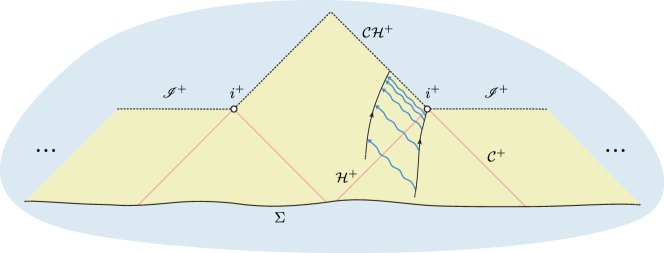
Figure 1: A schematic depiction of the blueshift instability in the case of a Reissner-Nordström-de Sitter black hole. Assume that radiation pulses at constant time intervals, as measured in proper time, from a timelike curve in the exterior of the black hole. The wordline in the exterior of the black hole has infinite affine length. On the other hand, observers along the timelike worldline in the black hole interior can reach the Cauchy horizon $\mathcal{CH}^{+}$ in finite proper time, thus receiving an infinite amount of pulses at the moment of crossing $\mathcal{CH}^{+}$.

Applying this insight to the full non-linear problem, however, is technically challenging. A turning point was the adoption of the Einstein-Maxwell-(real) scalar field model to study black hole interiors [Daf03], following previous work by Israel and Poisson [PI90]. Indeed, such a spherically symmetric (non-linear) toy model is able to efficiently describe the effects of Price’s law and of back-reaction, while at the same time capturing essential traits of the general setting. The addition of a scalar field, in particular, is motivated by the hyperbolic properties expected from the Einstein equations, and removes the constraints imposed by Birkhoff’s theorem. Inspired by this setting, the analysis of the non-linear problem in the absence of spherical symmetry was initiated only in the past few years [DL17]. We will review relevant past work in section 1.4.

Subsequently, several formulations of the SCCC have been advanced, depending on the required regularity of the extended metric as a solution to the Einstein equations. All these versions of the SCCC concern generic initial data.

While the existence of generic $C^{2}$ extensions represents a failure of determinism in the strongest sense, their absence does not prevent the occurrence of less regular extensions. Moreover, the $C^{2}$ level of regularity is seldom the most natural requirement. A discontinuous energy-momentum tensor in the Einstein equations typically appears for many physically relevant matched spacetimes, and can be related to solutions endowed with a $C^{1}$ metric.

On the other hand, the lack of continuous extensions entails unbounded geodesic deviation when reaching the boundary of the future domain of dependence (this is what occurs at the $r=0$ singularity in the Schwarzschild spacetime [Sbi18]). A further case is the $H^{1}_{\text{loc}}$ (Christodoulou-Chruściel) regularity, which is the minimal requirement to make sense of extensions as weak solutions to the Einstein equations (see also [CGNS18, DS18, Chr09, Chr91]), even though local well–posedness is not known to hold in this case [KRS15]. Weaker formulations can also be considered [Rei23]. We stress that showing the existence of an extension beyond the Cauchy horizon does not suffice to verify that such an extension satisfies the Einstein equations, but it is however a prerequisite for such a task. Moreover, proving that a particular, e.g. $C^{0}$, extension is not $C^{1}$ does not forbid the existence of other distinct $C^{1}$ extensions. An efficient way to rule out the latter might be to show the blow-up of a geometric $C^{1}$ quantity. This is the case of the Hawking mass in the works [PI90, Daf05a, CGNS18], for instance.

We stress that each formulation of the SCCC has to take into account the symmetries of the system and the nature of the adopted initial value problem, see also section 1.3 for a related discussion. Although we do not show that the initial conditions of our system arise from the evolution of initial data from an appropriate spacelike Cauchy hypersurface, our work provides strong evidence against general formulations of the SCCC. In particular, the content of this article is strictly related to the following conjectures.

Conjecture 1.1 ($C^{0}$ formulation of the SCCC for the Einstein-Maxwell-charged-Klein-Gordon system with $\Lambda>0$, under spherical symmetry)

Let $\Sigma$ be a regular, compact (without boundary), spacelike hypersurface. Let us prescribe generic (in the spherically symmetric class) initial data on $\Sigma$, for the Einstein-Maxwell-charged-Klein-Gordon system with $\Lambda>0$. Then, the future maximal globally hyperbolic development of such initial data cannot be locally extended as a Lorentzian manifold endowed with a continuous metric.

Conjecture 1.2 ($H^{1}_{\text{loc}}$ formulation of the SCCC for the Einstein-Maxwell-charged-Klein-Gordon system with $\Lambda>0$, under spherical symmetry)

Let $\Sigma$ be a regular, compact (without boundary), spacelike hypersurface. Let us prescribe generic (in the spherically symmetric class) initial data on $\Sigma$, for the Einstein-Maxwell-charged-Klein-Gordon system with $\Lambda>0$. Then, the future maximal globally hyperbolic development of such initial data cannot be locally extended as a Lorentzian manifold endowed with a continuous metric and Christoffel symbols in $H^{1}_{\text{loc}}$.

In particular, this work contributes to fill a gap in the literature by suggesting a negative resolution to conjecture 1.1 and, more significantly, a negative resolution, for a large subset of the parameter space, to conjecture 1.2. Being a natural generalization of [CGNS18] (but notice that the coupled scalar field is now charged and possibly massive) and [Moo18] (in our case, however, $\Lambda>0$, thus the Price law is exponential rather than inverse polynomial), we take these works as starting points for our analysis. In section 1.4 we review previous relevant work and compare the techniques we employed with those of [CGNS18] and [Moo18].

1.2 Summary of the main results

The main conclusions of our work can be outlined as follows. We first study the characteristic initial value problem (IVP) for the first-order system related to (1.1) (this corresponds to equations (2.20)–(2.33)) and establish its local well-posedness, modulo diffeomorphism invariance (see theorem 3.2 and proposition 3.4). We then provide a novel proof of the extension criterion for the first-order system (theorem 4.1), demanding less regularity on the initial data as compared to the analogous result in [Kom13, theorem 1.8] for the second-order system.

Subsequently, we show the equivalence between the first-order and the second-order Einstein-Maxwell-charged-Klein-Gordon systems (see remark 3.5) under additional regularity of the initial data, which we assume for the remaining part of our work. Finally, we assess the global uniqueness of the dynamical black hole under investigation, and its consequences for SCCC, in the following classes of regularity.

Theorem (stability of the Cauchy horizon and existence of continuous extensions. See corollary 5.21, theorem 5.22)

Let $Q_{+}$, $\varpi_{+}$ and $\Lambda$ be, respectively, the charge, mass and cosmological constant associated to a fixed sub-extremal Reissner-Nordström-de Sitter black hole. Let us consider, with respect to the first-order system (2.20)–(2.33), the future maximal globally hyperbolic development $(\mathcal{M},g,F,\phi)$ of spherically symmetric initial data prescribed on two transversal null hypersurfaces, where $q\in\mathbb{R}\setminus\{0\}$ is the charge of the scalar field $\phi$ and $m\geq 0$ its mass.

In particular, given $\mathcal{Q}=\mathcal{M}/SO(3)$, let $(u,v)$ be a system of null coordinates on $\mathcal{Q}$, determined by (2.44) and (2.45) and such that

$$g=-\Omega^{2}(u,v)dudv+r^{2}(u,v)\sigma_{S^{2}},$$ (1.2)

where $\sigma_{S^{2}}$ is the standard metric on the unit round sphere. For some $U>0$ and $v_{0}>0$, we express the two initial hypersurfaces in the above null coordinate system as $[0,U]\times\{v_{0}\}\cup\{0\}\times[v_{0},+\infty)$.

Assume that the initial data to the characteristic IVP satisfy assumptions (A)–(G), which require, in particular, that the initial data asymptotically approach those of the afore-mentioned sub-extremal black-hole, and that an exponential Price law upper bound holds: there exists $s>0$ and $C>0$ such that

$$|\phi|(0,v)+|\partial_{v}\phi|(0,v)\leq Ce^{-sv}.$$ (1.3)

Then, if $U$ is sufficiently small, there exists a unique solution to this characteristic IVP, defined on $[0,U]\times[v_{0},+\infty)$, given by metric (1.2) and such that

$$u\mapsto\lim_{v\to+\infty}r(u,v)\geq\mathfrak{r}>0$$

is a continuous function from $[0,U]$ to $[\mathfrak{r},r_{-}]$, for some $\mathfrak{r}>0$, and

$$\lim_{u\to 0}\lim_{v\to+\infty}r(u,v)=r_{-},$$

where $r_{-}$ is the radius of the Cauchy horizon of the reference sub-extremal Reissner-Nordström-de Sitter black hole.

Moreover, $(\mathcal{M},g,F,\phi)$ can be extended up to the Cauchy horizon $\mathcal{CH}^{+}=\{v=+\infty\}$ with continuous metric and continuous scalar field $\phi$.

This suggests a negative resolution to conjecture 1.1 (see also section 1.3), for every non-zero value of the scalar field charge and for every non-negative value of its mass.

Theorem (no-mass-inflation scenario and $H^{1}$ extensions. See theorems 6.1 and 6.6)

Under the assumptions of the previous theorem, let $s$ be the constant in (1.3) and consider

$$\rho\coloneqq\frac{K_{-}}{K_{+}}>1,$$

where $K_{-}$ and $K_{+}$ are the surface gravities of the Cauchy horizon and of the event horizon, respectively, of the reference sub-extremal Reissner-Nordström-de Sitter black hole. We define the renormalized Hawking mass

$$\varpi=\frac{r}{2}\left(1-g(dr^{\sharp},dr^{\sharp})\right)+\frac{Q^{2}}{2r}-\frac{\Lambda}{6}r^{3},$$

where $Q$ is the charge function of the dynamical black hole and $\Lambda$ is the cosmological constant. If:

$$s>K_{-}\quad\text{and}\quad\rho<2,$$ (1.4)

then the geometric quantity $\varpi$ is bounded, namely there exists $C>0$, depending uniquely on the initial data, such that:

$$\|\varpi\|_{L^{\infty}([0,U]\times[v_{0},+\infty))}=C<+\infty.$$

Moreover, for such values of $s$ and $\rho$, there exists a coordinate system for which $g$ can be extended continuously up to $\mathcal{CH}^{+}$, with Christoffel symbols in $L^{2}_{\text{loc}}$ and $\phi$ in $H^{1}_{\text{loc}}$.

When the decay given by the exponential Price law upper bound is sufficiently fast and the parameters of the reference sub-extremal black hole lie in a certain range, the above result puts into question the validity of conjecture 1.2 (see also section 1.3).

As showed in Fig. 2, this theorem significantly extends the range of parameters for which $H^{1}$ extensions can be obtained, when comparing to the case of a massless and uncharged scalar field [CGNS18], in a way which is expected to be sharp in the $(s,\rho)$ parameter space [CF17, HV17]. We stress that the range of parameters allowing for $H^{1}$ extensions is not expected to depend on the charge of the scalar field. On the other hand, the techniques of the present paper are more general than those previously used in the case of an uncharged scalar field case, when $\Lambda>0$. In particular, our methods can be applied to the uncharged case as well.

Notice that the first condition in (1.4) depends on the choice of the outgoing null coordinate $v$, see also appendix B.

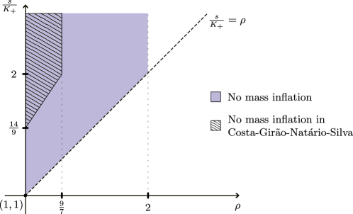
Figure 2: Values of $s$ and $\rho=\frac{K_{-}}{K_{+}}$ that guarantee absence of mass inflation for a generic set of initial data, in comparison to the results in [CGNS18]. In the extended range that we obtained, $H^{1}_{\text{loc}}$ extensions of the solutions to the IVP are constructed. This extended range includes near-extremal black holes, for which $\rho$ is close to 1. The value of $s$ is expected to depend in a non-trivial way on the parameters of the fixed sub-extremal black hole, see [CCDHJ18, CCDHJ18a, Hin21, HX22, CM22].

1.3 Strong cosmic censorship in full generality

The results of our analysis show that the main conclusion of [CGNS18] is still valid when we add a charge (and possibly mass) to the coupled scalar field: according to the state of the art of SCCC, the potential scenarios that lead to a violation of determinism in the case $\bm{\Lambda>0}$ cannot be ruled out.

To explain how to reach this conclusion, we first illustrate the connection between our results and conjecture 1.2, and then the relation between the latter and other formulations of SCCC.

The results presented in section 1.2 stem from the evolution of initial data from two transversal null hypersurfaces, one of which modelling the event horizon of a dynamical black hole. This suggests that the black hole we take under consideration has already formed at the beginning of the evolution.

Strictly speaking, however, SCCC constrains the admissible future developments of spacelike hypersurfaces, on which generic initial data are specified. Although we are not committed to any specific global structure, it is useful to think of the characteristic IVP of section 2.1 as arising from suitable (compact or non-compact) initial data prescribed in the black hole exterior (see also Fig. 3). The reason why we believe that our results are relevant to SCCC is that the initial data we prescribe for our characteristic IVP are compatible with numerical solutions obtained in the exterior of Reissner-Nordström-de Sitter black holes. Such results are also expected to hold for perturbations of such black holes, due to the non-linear stability result [Hin18].

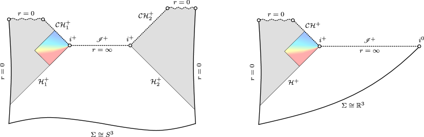
Figure 3: Two possible global spacetime structures in which the characteristic IVP of section 2.1 fits in. The coloured region is the one depicted in the forthcoming Fig. 4, namely the black hole interior region under inspection in the present work. These global structures require a dynamical formation of trapped surfaces, starting from non-trapped initial data (see also [Cos20, AL22]).

In particular, our $v$ coordinate can be compared to half of the outgoing Eddington-Finkelstein coordinate of [CCDHJ18a] (see appendix B). This can be used to see that, according to the same article, condition (1.4) can be (numerically) attained at the linear level: $s>K_{-}$ (i.e. $\beta=\frac{s}{2K_{-}}>\frac{1}{2}$, in the language of [CCDHJ18a]) for linear waves propagating in the exterior of near-extremal (i.e. $\rho$ close to 1) Reissner-Nordström-de Sitter black holes. This result is also expected to hold on dynamical black holes sufficiently close to Reissner-Nordström-de Sitter, as the one we analyse. Indeed, notice that on a fixed background $s$ is equal, up to a multiplying factor, to the spectral gap of the Laplace-Beltrami operator $\square_{g}$. If we denote by QNM the set of the quasinormal modes of the reference black hole, the spectral gap can also be expressed by

$$\inf_{\begin{subarray}{c}\omega\in\text{QNM}\\ \operatorname{Im}(\omega)<0\end{subarray}}\left(-\operatorname{Im}(\omega)\right).$$

In particular, $s$ depends on the black hole parameters. At the same time, [Hin18] shows that, under small perturbations, the parameters of the perturbed solution are sufficiently close to the initial ones.

Therefore, once the numerical results of [CCDHJ18a] are verified rigorously and extended to the non-linear case, a mathematical proof for the validity of (1.4) would in principle be possible, leading to a negative resolution of conjecture 1.2.

On the other hand, conjectures 1.1 and 1.2 regard initial data which are generic in the spherically symmetric class, but non-generic in the much larger moduli space of all possible initial configurations. In particular, when we talk about SCCC under spherical symmetry, the validity or failure of such a conjecture does not automatically settle the non-spherically symmetric problem. Nonetheless, due to analogies with the conformal structure of a Kerr-Newman spacetime, it is widely believed [Daf03, Daf05a, CGNS18, DL17] that results obtained in the charged spherically symmetric context can provide vital evidence to either uphold or refute formulations of SCCC in absence of spherical symmetry.

A larger moduli space can also be achieved by working in a rougher class of initial data. In [DS18], where global uniqueness is investigated at the linear level, the following is proved: given initial data $(\psi_{0},\psi_{0}^{\prime})\in H^{1}_{\text{loc}}\times L^{2}_{\text{loc}}$ to the linear wave equation $\square_{g}\psi=0$ on a sub-extremal Reissner-Nordström-de Sitter black hole, with data prescribed on a complete spacelike hypersurface, $\psi$ cannot be extended across the Cauchy horizon in $H^{1}_{\text{loc}}$. This means that, if the numerical results [CCDHJ18] obtained in the exterior of Reissner-Nordström-de Sitter black holes were to be proved rigorously, the initial data leading to a potential failure of SCCC could be ignored, because they are non-generic in this larger set of rough initial configurations. Whether this Sobolev level of regularity for the initial data is “suitable” may well depend on the problem to be studied and is still a topic of discussion in the literature.

1.4 Previous works and outline of the bootstrap method

The case $\bm{\Lambda=0}$: after foundational work by Christodoulou [Chr99], Dafermos [Daf03] first laid the framework for the analysis of the SCCC in spherical symmetry via modern PDE methods. With the long-term motivation of probing the stability of the Cauchy horizon for a Kerr black hole, he studied the Einstein-Maxwell-(real) scalar field system as a proxy to the full non-linear problem. This first pioneering work concerned a characteristic initial value problem where Reissner-Nordström initial data (and a zero scalar field) were assumed on the initial outgoing characteristic hypersurface. The direct analogy between the conformal structure of the interior of Kerr and that of the Reissner-Nordström solution indeed supports the choice of the latter model as a representative of the behaviour of the rotating black hole.

Apart from spherical symmetry, two artificial elements are included in this framework: the scalar field is taken real-valued, thus restricting the analysis to solutions expected to arise from two-ended, asymptotically flat, initial data [Kom13]. On the other hand, the scalar field is assumed to vanish identically along the initial outgoing hypersurface, so that Reissner-Nordström initial data are prescribed there.

The latter assumption was replaced in [Daf05a], where the $C^{0}$ version of SCCC was proved to be false, conditionally on the validity of a Price law upper bound, which was later seen to hold in [DR05]. In [Daf05a], the $C^{1}$ formulation of SCCC was seen to hinge on the validity of a lower bound on the scalar field along the event horizon. The work [LO19], again on the Einstein-Maxwell-(real) scalar field system under spherical symmetry, ascertained the validity of the $C^{2}$ formulation of SCCC. This was achieved by proving that an integrated lower bound holds generically for the scalar field and that this leads to a curvature blow-up, identically along the Cauchy horizon.

The first steps towards the analysis of a complex-valued (i.e. charged) and possibly massive scalar field were taken in [Kom13]: this is the model that we denoted as the Einstein-Maxwell-charged-Klein-Gordon system. The work [Kom13], in particular, presented a soft analysis of the future boundary of spacetimes undergoing spherical collapse. More recent work on the SCCC for the same system can be found in [Moo18, Moo22, Moo21, KM22], where continuous spacetime extensions were constructed and several instability results obtained.

The analysis of the full non-linear problem, namely the validity of the SCCC for a Kerr spacetime, was initiated in the seminal work [DL17]. Here, the $C^{0}$ formulation of the SCCC was shown to be false, under the assumption of the quantitative stability of the Kerr exterior. The problem is indeed intertwined with stability results of black hole exteriors, object of an intense activity that built on a sequence of remarkable results and notably led, in recent times, to [GKS22, KS21, KS22] for slowly rotating Kerr solutions. Further celebrated results are the non-linear stability of the Schwarzschild family [DHRT21] and, in the case $\Lambda>0$, the non-linear stability of slowly rotating Kerr-Newman-de Sitter black holes [Hin18]. For an overview on the problem and recent contributions both in the linear and non-linear realm, we refer the reader to [AB15, HHV21, Mos20, Gio20, Ben22, Tei20] and references therein.

The case $\bm{\Lambda>0}$: Compared to the asymptotically flat scenario, the presence of a positive cosmological constant leads to substantial changes in the causal structure of black hole solutions. A Reissner-Nordström-de Sitter black hole, for instance, presents a spacelike future null infinity and an additional Killing horizon $\mathcal{C}^{+}$ (the cosmological horizon). As a result, scalar perturbations of such a black hole decay exponentially fast along $\mathcal{H}^{+}$ [Dya15]. This behaviour competes with the blueshift effect expected near the Cauchy horizon and determining a growth, also exponential, of the main perturbed quantities. While SCCC is expected to prevail in the asymptotically flat case (the exponential contribution from blueshift wins over the inverse polynomial tails propagating from the event horizon), the situation drastically changes when $\Lambda>0$. In the latter case, indeed, knowing the exact asymptotic rates of scalar perturbations along the event horizon, and thus determining which of the two exponential contributions is the leading one, is of vital importance to determine the admissibility of spacetime extensions. For instance, a sufficiently rapid decay given by the Price law is expected to overcome the blueshift effect and allow observers to cross the Cauchy horizon without significant obstructions. So far, a quantitative description of the exponents for such a decay is available at the linear level via numerical methods [CCDHJ18, CCDHJ18a, CM22, MTWZZ18], whereas rigorous results are mostly lacking (see however [Hin21] and [HX22] where Kerr and Schwarzschild solutions with positive $\Lambda$ have been studied in the case of small black hole mass or small cosmological constant). In this work, all possible exponential rates along the event horizon are taken into consideration.

Similarly to the case of a zero cosmological constant, the SCCC with $\Lambda>0$ has also been studied via the Einstein-Maxwell-(real) scalar field model. The works [CGNS15, CGNS15a, CGNS17] can be compared to [Daf03]: a characteristic initial value problem was studied, with data on the initial outgoing hypersurface given by the event horizon of a Reissner-Nordström-de Sitter black hole. One of the main novelties of this series of papers is a partition of the black hole interior in terms of level sets of the radius function, rather than curves of constant shifts as in [Daf03, Daf05a] (the latter curves fail to be spacelike when $\Lambda\neq 0$). These three works deal with a real scalar field, taken identically zero along the event horizon. Conversely, an exponential Price law (both a lower bound and an upper bound) was prescribed in [CGNS18] along the event horizon (compare with [Daf05a]), and generic initial data leading to $C^{0}$ extensions were constructed. Conditions to have either $H^{1}_{\text{loc}}$ extensions or mass inflation where given in terms of the decay of the scalar field along the event horizon.

The work that we present in the next sections is a natural prosecution of [CGNS18] as it replaces the neutral scalar field with a charged one, whose behaviour along the event horizon is dictated by an exponential Price law upper bound. Differently from [CGNS18], however, we are able to prove stability results in the charged case without requiring a Price law lower bound, and we extend, in a way which is expected to be optimal, the set of parameters $s$ and $\rho$ that allow for $H^{1}_{\text{loc}}$ extensions.

On a more technical level, we stress that the exponential Price law is prescribed as a consequence of the positivity of the cosmological constant. On the other hand, our computations show that the sign of $\Lambda$ does not affect the conclusions of this work.

We also mention the numerical works [CCDHJ18, CCDHJ18a], which inspected the effects of linear scalar perturbations on sub-extremal Reissner-Nordström-de Sitter black holes. For a charged scalar field, numerical evolutions suggest that there exist values for the scalar field charge and the final black hole charge for which the (Christodoulou-Chruściel) SCCC is violated at the linear level. A different outcome was found in the Kerr-de Sitter case [DERS18], where numerical results showed that $H^{1}_{\text{loc}}$ SCCC is respected in the linear setting. An extension of these results to regions of the Kerr-Newman family was presented in [CM22].

The case $\bm{\Lambda<0}$ and extremal black holes: recent progress with the investigation of SCCC both for the case $\Lambda<0$ and for extremal black holes can be found, for instance, in [HS13, Keh22, Mos20] and [Are11, AAG23].

Comparison with [Moo18] and [CGNS18]: the present work generalizes the results of [CGNS18] to the case of a charged and (possibly) massive scalar field, without requiring any lower bound for it along the initial outgoing characteristic hypersurface. Differently from the neutral case, a charged scalar field is compatible with a more realistic description of gravitational collapse (see Fig. 3 for potential global structures). At the same time, the charged setting requires gauge covariant derivatives, brings additional terms in the equations and generally undermines monotonicity properties due to the fact that the scalar field is now complex-valued. With respect to the real case, additional dynamical quantities, such as the electromagnetic potential $A_{u}$ and the charge function $Q$, need to be controlled during the evolution. Moreover, the scalar field is expected to oscillate along the event horizon of the dynamical black hole: the pointwise Price law lower bound used in [CGNS18] to prove instability results is too restrictive to be replicated in the current case. The presence of a mass term for the scalar field, on the other hand, allows to describe compact objects formed by massive spin-0 bosons.

In particular, we replace many monotonicity arguments exploited in [CGNS18] with bootstrap methods. In this sense, our work follows the spirit of [Moo18], where the stability of the Cauchy horizon was proved by bootstrapping the main estimates from the event horizon. However, as we will see, the techniques we use to close the bootstrap arguments differ more and more from the ones of [Moo18] as we approach the Cauchy horizon. More specifically, we subdivide the black hole interior into five regions: these are the event horizon, the redshift region, the no-shift region, the early blueshift region and the late blueshift region. The subdivision is given in terms of curves of constant area-radius, as in [CGNS15a, CGNS17, CGNS18]. This partition is loosely analogous to the one performed in [Moo18], which is the source for this nomenclature, in the sense that both constructions measure the redshift and blueshift effects in a similar fashion. This analogy, however, is only meaningful if the different values of the cosmological constant are taken into account (inverse polynomial decay rates need to be replaced by exponential ones and vice versa). Indeed, differently from [Moo18], the exponential Price law in our work gives exponential terms in the main estimates, that compete against the decay rate given by the redshift effect and the exponential growth near the Cauchy horizon, due to blueshift. This is exemplarily represented by the loss of decay in the redshift region, compared to the event horizon, for solutions to the IVP.

We expand the results of [CGNS18] to the case of a charged and possibly massive scalar field. In particular being able to prove the existence of $H^{1}_{\text{loc}}$ extensions beyond the Cauchy horizon in a larger set of black hole parameters, in a way which is expected to be sharp according to the linear theory [CF17, HV17]. We stress that the only restrictions on the scalar field charge $q$ and mass $m$ are given by $q\neq 0$ and $m\geq 0$.

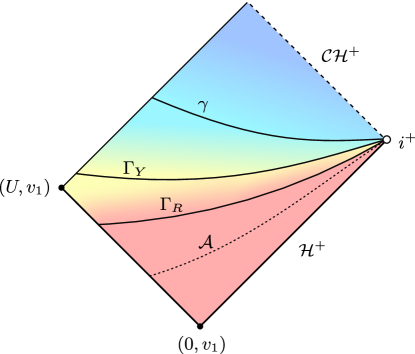
Figure 4: A posteriori, these are the spacelike curves that partition the interior of the dynamical black hole for $v_{1}\geq v_{0}$ large. Compare with Fig. 3 in [Moo18] and with the figures in [CGNS18, section 4]. For the construction, we consider $r_{-}$ and $r_{+}$, with $0<r_{-}<r_{+}$, respectively the radius of the Cauchy horizon and the radius of the event horizon of the reference sub-extremal black hole. For $\delta$ and $\Delta$ positive and small, we fix $R\in(r_{+}-\delta,r_{+})$ and $Y\in(r_{-},r_{-}+\Delta)$. The region to the past of $\Gamma_{R}=\{r=R\}$ is the redshift region (the curve $\mathcal{A}$ is the apparent horizon). Between $\Gamma_{R}$ and $\Gamma_{Y}=\{r=Y\}$ is the no-shift region. Bounded between $\Gamma_{Y}$ and $\gamma$ (which is not a level set of $r$) is the early blueshift region. Finally, to the future of $\gamma$ we have the late blueshift region.

We now summarize the main technical strategies that we adopt in each region of the black hole interior (see also Fig. 4). Here, the quantities $r_{-}$ and $r_{+}$ represent the radii of the Cauchy horizon and of the event horizon, respectively, of the fixed sub-extremal Reissner-Nordström-de Sitter black hole. We recall that in section 1.2 we presented the coordinates $u$ and $v$ and the function $\Omega^{2}$ (see (1.2)). The function $\mu$ is defined in (2.16).

• Event horizon, section 5.1: the exponential Price law gives an upper bound on the scalar field, determined by the term $e^{-sv}$, for a fixed $s\in(0,+\infty)$. We then obtain an exponentially fast convergence of the main dynamical quantities to those of the reference Reissner-Nordström-de Sitter black hole. We mainly follow [Moo18] for this result (there, the convergence is inverse polynomial since $\Lambda$ is zero).

• Redshift region, section 5.3: this is the region bounded between the event horizon and the curve of constant radius $R$, where $0<r_{+}-R<\delta$, for some small $\delta>0$. Here, the redshift effect competes with the exponential Price law. This is translated into the presence of the slower decay rate $e^{-c(s)v}$, rather than $e^{-sv}$. The monotonicity results and Grönwall inequalities adopted in the real-scalar-field case are replaced by a bootstrap argument, which can be closed by using the smallness of the geometric quantity $|r-r_{+}|$. This differs from the case of [Moo18], where the coordinate-dependent quantity $U\Omega^{2}(0,v)$ is the one assumed small in the analogous region. An advantage of our construction is that the control on the radius function $r$ follows automatically. This is particularly relevant here since the cosmological constant is always coupled to a function of $r$ in the main equations of our PDE system. The definition of $c(s)$ and the bootstrap procedure is planned so as to deal with the competition between the two exponentially decaying terms.

• No-shift region, section 5.5: the past of this region is bounded by the curve $\Gamma_{R}$, while the future is determined by $\Gamma_{Y}$, where $0<Y-r_{-}<\Delta$ for some small $\Delta>0$. Since the distance between $r$ and either $r_{+}$ or $r_{-}$ is bounded, but not necessarily small, the bootstrap argument of the previous region does not apply. Instead, we further divide this set into finitely many subregions in which we have a finer control on the area-radius function. We deduce the main estimates on each subregion by induction, where the inductive step is proved by bootstrap. A similar technique was also used in [Moo18]. The core point of the proof consists of bounding the negative quantity $1-\mu$ away from zero, as done in [CGNS18]. Differently from the latter paper, however, the monotonicity properties of $\varpi$ are now lacking. In their place, we exploit bootstrap arguments.

• Early blueshift region, sections 5.6 and 5.7: it is enclosed by the curves

  $$\Gamma_{Y}=\{(u,v_{Y}(u))\colon u\in[0,U]\}$$

  and

  $$\gamma=\{(u,(1+\beta)v_{Y}(u))\colon u\in[0,U]\},$$

  for some $\beta>0$. The full description of such curves is given in section 5.6. In particular, the curve $\gamma$ (already defined in [CGNS18]) has the main purpose to probe the blueshift effect. Differently from [CGNS18, Daf05a], BV estimates cannot be easily obtained, due to additional terms appearing in the main equations for $\partial_{v}\phi$ and $D_{u}\phi$. The problem is again solved by bootstrap, where the argument can be closed by assuming that $\Gamma_{Y}$ and $\gamma$ are sufficiently close to $\Gamma_{r_{-}}$. Moreover, an exponentially growing contribution is now competing with the exponential decays that we have propagated from $\mathcal{H}^{+}$. To guarantee a decaying behaviour, we use the closeness of the curve $\gamma$ to $\Gamma_{Y}$. We stress that, in [Moo18], the number of subregions of the no-shift region times the smallness parameter used in such a region could be taken large, with the aim of closing the bootstrap argument. This is not possible in our case, since such a value is a constant and is equal to $R-Y$, again due to our construction in terms of constant-radius curves. The main novel idea in this region consists of propagating an exponential decay depending on both null coordinates. This has the objective to interpolate between the decay rates obtained in the no-shift region and the ones expected along the curve $\gamma$ due to the contribution of blueshift.

• Late blueshift region, section 5.8: this coincides with the causal future of $\gamma$. The soft arguments used in [CGNS18] to propagate the known estimates do not apply here, due to the presence of a non-constant charge function $Q$. Therefore, we propagate the main estimates by bootstrap again. The bootstrap technique is different from the one of the previous regions, since we have less control on the quantities $\phi$ and $D_{u}\phi$. A key role in the bootstrap argument is played by an estimate on $\partial_{v}\log\Omega^{2}$, which we propagate from the event horizon and is used essentially only in this region. This quantity measures, in some sense, the redshift and blueshift effects. It was used repeatedly in [Moo18] to show the existence of $C^{0}$ extensions. Furthermore, in contrast with [CGNS18], we are able to obtain a finer control on the $H^{1}$ norm of the scalar field. This allows us to provide a larger generic set of initial data, with respect to [CGNS18], for which mass inflation can be prevented and $H^{1}_{\text{loc}}$ extensions can be obtained.

The outline of the paper is the following: in section 2 we delve into the main aspects of the characteristic IVP for the Einstein-Maxwell-charged-Klein-Gordon system under spherical symmetry. Well-posedness of the characteristic IVP is investigated in section 3. An extension criterion is given in section 4.

In section 5 we establish quantitative bounds along $\mathcal{H}^{+}$ for the main PDE variables of the characteristic IVP, and propagate these bounds to the black hole interior by bootstrap. This allows us to prove the stability of $\mathcal{CH}^{+}$ and to construct a continuous spacetime extension at the end of the same section.

In section 6 we provide a sharp condition on the reference sub-extremal black hole to generically prevent the occurrence of mass inflation. Under such an assumption, we also construct an $H^{1}_{\text{loc}}$ spacetime extension up to and including the Cauchy horizon.

1.5 Acknowledgements

The author is grateful to his PhD supervisors João Costa and José Natário for suggesting the problem and for their invaluable guidance and advice while completing the manuscript. The author would also like to thank Ryan Unger for insightful comments on the manuscript. This work was supported by FCT/Portugal through the PhD scholarship UI/BD/152068/2021, and partially supported by FCT/Portugal through CAMGSD, IST-ID, projects UIDB/04459/2020 and UIDP/04459/2020.

2 The Einstein-Maxwell-charged-Klein-Gordon system under spherical symmetry

The present work revolves around the system of equations describing a spherically symmetric Einstein-Maxwell-charged-Klein-Gordon model with positive cosmological constant $\Lambda$:

$$\begin{cases}\text{Ric}_{\mu\nu}(g)-\frac{1}{2}\text{R}(g)g_{\mu\nu}+\Lambda g_{\mu\nu}=2\left(T^{\text{EM}}_{\mu\nu}+T^{\phi}_{\mu\nu}\right),\\[3.00003pt] T^{\text{EM}}_{\mu\nu}=g^{\alpha\beta}F_{\alpha\mu}F_{\beta\nu}-\frac{1}{4}g_{\mu\nu}F^{\alpha\beta}F_{\alpha\beta},\\[3.00003pt] T^{\phi}_{\mu\nu}=\operatorname{Re}\left(D_{\mu}\phi\overline{D_{\nu}\phi}\right)-\frac{1}{2}g_{\mu\nu}\left(D_{\alpha}\phi\overline{D^{\alpha}\phi}+m^{2}|\phi|^{2}\right),\\[3.00003pt] dF=0,\quad d\star F=\star J,\\[3.00003pt] \left(D_{\mu}D^{\mu}-m^{2}\right)\phi=0.\end{cases}$$

The above system describes a spherically symmetric spacetime $(\mathcal{M},g)$ interacting with a scalar field $\phi$, the latter being endowed with charge $q\in\mathbb{R}\setminus\{0\}$ and mass $m\geq 0$. The units are chosen so that $c=4\pi G=\epsilon_{0}=1$ and the symbol $\star$ denotes the Hodge-star operator. The charge generates an electromagnetic field which interacts with the spacetime itself and is modelled by the strength field tensor $F$. The description of the charged scalar field through a complex-valued function and the use of the gauge covariant derivative

$$D_{\mu}=\nabla_{\mu}+iqA_{\mu}$$ (2.1)

are standard techniques in the gauge-theoretical framework (see [Kom13] for more details) and in Lagrangian formalism. The current

$$J_{\mu}=-\frac{iq}{2}\left(\phi\overline{D_{\mu}\phi}-\overline{\phi}D_{\mu}\phi\right)$$ (2.2)

appearing in Maxwell’s equations, in particular, can be seen as the Noether current of the (classical) Lagrangian density $\mathcal{L}=|D_{\mu}\phi|^{2}-m^{2}|\phi|^{2}$.

We express the isometric action of $SO(3)$ on our spacetime manifold by assuming

$$g=g_{\mathcal{Q}}+r^{2}(u,v)\sigma_{S^{2}},$$ (2.3)

with

$$g_{\mathcal{Q}}\coloneqq-\Omega^{2}(u,v)dudv,$$

for some real-valued function $\Omega$, where $\sigma_{S^{2}}=d\theta^{2}+\sin^{2}(\theta)d\varphi^{2}$ is the standard metric on the unit round 2-sphere, $r$ is the area-radius function and $u,v$ are null coordinates in the $(1+1)$–dimensional manifold $\mathcal{Q}\coloneqq\mathcal{M}/SO(3)$. In particular, we can conformally embed $(\mathcal{Q},g_{\mathcal{Q}})$ in $(\mathbb{R}^{2},\eta)$, where $\eta$ is the Minkowski metric, and we can restrict ourselves to working with this subset of the two-dimensional space since conformal transformations preserve the causal structure. Moreover, we will make use of the $U(1)$ gauge freedom to assume that $\phi$ and $A$ (see (2.1)) do not depend on the angular coordinates. We will also require that $\partial_{u}=\frac{\partial}{\partial u}$ is a future-pointing, ingoing vector field and $\partial_{v}$ is a future-pointing, outgoing one.

We use the same symbol to denote a spherically symmetric function defined on $\mathcal{M}$, and its push-forward through the projection map $\pi\colon\mathcal{M}\to\mathcal{Q}$.

In order to analyse the behaviour of our dynamical system, we are first naturally led to investigate the maximal globally hyperbolic development (MGHD) generated by (spherically symmetric) initial data prescribed on a suitable spacelike hypersurface (see also section 1.3 for possible global structures). After this analysis, the null structure of the equations motivates us to treat the characteristic initial value problem on $\mathcal{Q}$, using the $(u,v)$ coordinate system.

With respect to the afore-mentioned $(u,v)$ null coordinates, we are going to work in the set $[0,U]\times[0,+\infty)$, for some $U>0$. Therefore, there exists a 1-form $A$ defined on the MGHD of the initial data set, such that $F=dA=F_{uv}(u,v)du\wedge dv$ for some real-valued function $F_{uv}$. In particular, we can define the real-valued function $Q(u,v)$ such that

$$F=\frac{Q\Omega^{2}}{2r^{2}}du\wedge dv.$$ (2.4)

Since we can choose the electromagnetic potential $A$ up to an exact form by performing a gauge choice, we can set $A=A_{u}du$. Thus, the gauge covariant derivative $D_{v}$ is just $\nabla_{v}$ (see (2.1)) and

$$\partial_{v}{A_{u}}=-\frac{Q\Omega^{2}}{2r^{2}}.$$ (2.5)

The above expression defines $A_{u}$ up to a function of $u$. So, without loss of generality, we will assume that $A_{u}$ vanishes on the initial ingoing hypersurface. Namely, for $U>0$ and $v_{0}\geq 0$ fixed, we take $A_{u}(u,v_{0})=0$ for every $u\in[0,U]$.

2.1 The second-order and first-order systems: the characteristic initial value problem

Using the results of appendix A, we can write down the Einstein equations in the following form:

$$\partial_{u}{\left(\frac{\partial_{u}r}{\Omega^{2}}\right)}=-r\frac{\lvert D_{u}\phi\rvert^{2}}{\Omega^{2}},\quad\text{(Raychaudhuri equation along the }u\text{ direction),}$$ (2.6)

$$\partial_{v}{\left(\frac{\partial_{v}{r}}{\Omega^{2}}\right)}=-r\frac{\lvert\partial_{v}{\phi}\rvert^{2}}{\Omega^{2}},\quad\text{ (Raychaudhuri equation along the }v\text{ direction),}$$ (2.7)

$$\partial_{u}{\partial_{v}{r}}=\frac{\Omega^{2}}{4r^{3}}Q^{2}+\frac{\Omega^{2}r}{4}\Lambda-\frac{\Omega^{2}}{4r}-\frac{\partial_{v}{r}\partial_{u}{r}}{r}+\frac{m^{2}\Omega^{2}}{4}r|\phi|^{2},\quad\,\,\,\text{ (wave eqn.\ for }r\text{),}$$ (2.8)

$$\partial_{u}{\partial_{v}{\log\Omega^{2}}}=-2\operatorname{Re}{\left(D_{u}\phi\overline{\partial_{v}{\phi}}\right)}-\frac{\Omega^{2}Q^{2}}{r^{4}}+\frac{\Omega^{2}}{2r^{2}}+\frac{2\partial_{v}{r}\partial_{u}{r}}{r^{2}},\,\,\,\,\text{(wave eqn.\ for}\log\Omega^{2}\text{),}$$ (2.9)

Moreover, the equation of motion $\left(D_{\mu}D^{\mu}-m^{2}\right)\phi=0$ becomes

$$\partial_{u}{\partial_{v}{\phi}}=-\frac{1}{r}\left(D_{u}{r}\partial_{v}{\phi}+\partial_{v}{r}D_{u}{\phi}\right)+\frac{iqQ\Omega^{2}}{4r^{2}}\phi-\frac{m^{2}\Omega^{2}}{4}\phi,\quad\text{(Klein-Gordon equation)}$$ (2.10)

where we used that

$$\nabla_{\mu}\nabla^{\mu}\phi=-\frac{4}{r\Omega^{2}}\left(\partial_{u}{r}\partial_{v}{\phi}+\partial_{v}{r}\partial_{u}{\phi}+r\partial_{u}{\partial_{v}{\phi}}\right),$$

and

$$\nabla_{\mu}A^{\mu}=-\frac{2}{\Omega^{2}}\partial_{v}{A_{u}}-\frac{4}{\Omega^{2}r}A_{u}\partial_{v}{r}=\frac{Q}{r^{2}}-\frac{4}{\Omega^{2}r}A_{u}\partial_{v}{r}.$$

Furthermore, the second Maxwell equation $d\star F=\star J$ implies

$$\partial_{u}Q =-qr^{2}\operatorname{Im}\left(\phi\overline{D_{u}\phi}\right),$$ (2.11)

$$\partial_{v}Q =qr^{2}\operatorname{Im}\left(\phi\overline{\partial_{v}{\phi}}\right).$$ (2.12)

In order to study the well-posedness of our system of PDEs, it is useful to rewrite the above equations as a first-order system. To do this, we define the following quantities:

$$\nu \coloneqq\partial_{u}{r},$$ (2.13)

$$\lambda \coloneqq\partial_{v}{r},$$ (2.14)

which were first introduced by Christodoulou, and

$$\varpi \coloneqq\frac{Q^{2}}{2r}+\frac{r}{2}-\frac{\Lambda}{6}r^{3}+\frac{2r}{\Omega^{2}}\nu\lambda,$$ (2.15)

$$\mu \coloneqq\frac{2\varpi}{r}-\frac{Q^{2}}{r^{2}}+\frac{\Lambda}{3}r^{2},$$ (2.16)

$$\theta \coloneqq r\partial_{v}{\phi},$$ (2.17)

$$\zeta \coloneqq rD_{u}\phi,$$ (2.18)

$$\kappa \coloneqq-\frac{\Omega^{2}}{4\nu},$$ (2.19)

whenever $r$, $\Omega^{2}$ and $\nu$ are non-zero, an assumption that we will make on the initial hypersurfaces of our PDE system. All the newly defined quantities are real-valued, except for $\theta$ and $\zeta$, since the scalar field $\phi$ is complex-valued. From the above we can obtain the useful relation

$$\lambda=\kappa(1-\mu).$$

We also notice that $\varpi$ is a geometric quantity (often called the renormalized Hawking mass), due to the fact that $1-\mu=g(dr^{\sharp},dr^{\sharp})$. Using the new definitions, some lines of computations show that the Einstein, Klein-Gordon and Maxwell equations imply the following first-order system:

$$\partial_{u}{r} =\nu,$$ (2.20)

$$\partial_{v}{r} =\lambda,$$ (2.21)

$$D_{u}\phi=\left(\partial_{u}+iqA_{u}\right)\phi =\frac{\zeta}{r},$$ (2.22)

$$D_{v}\phi=\partial_{v}{\phi} =\frac{\theta}{r},$$ (2.23)

$$\partial_{v}{\nu}=\partial_{u}{\lambda} =-2\nu\kappa\frac{1}{r^{2}}\left(\frac{Q^{2}}{r}+\frac{m^{2}r^{3}|\phi|^{2}}{2}+\frac{\Lambda}{3}r^{3}-\varpi\right),$$ (2.24)

$$\partial_{u}{\varpi} =\frac{\nu}{2}m^{2}r^{2}|\phi|^{2}-Qq\operatorname{Im}{\left(\phi\overline{\zeta}\right)}+\frac{1}{2}\left(\frac{|\zeta|}{\nu}\right)^{2}\nu\left(1-\frac{2\varpi}{r}+\frac{Q^{2}}{r^{2}}-\frac{\Lambda}{3}r^{2}\right),$$ (2.25)

$$\partial_{v}{\varpi} =\frac{\lambda}{2}m^{2}r^{2}|\phi|^{2}+Qq\operatorname{Im}{\left(\phi\overline{\theta}\right)}+\frac{|\theta|^{2}}{2\kappa},$$ (2.26)

$$D_{u}\theta=\left(\partial_{u}+iqA_{u}\right)\theta =-\frac{\zeta}{r}\lambda+\frac{\nu\kappa\phi}{r}\left(m^{2}r^{2}-iqQ\right),$$ (2.27)

$$D_{v}\zeta=\partial_{v}{\zeta} =-\frac{\theta}{r}\nu+\frac{\nu\kappa\phi}{r}\left(m^{2}r^{2}+iqQ\right),$$ (2.28)

$$\partial_{u}{\kappa} =\frac{\kappa\nu}{r}\left(\frac{|\zeta|}{\nu}\right)^{2},$$ (2.29)

$$\partial_{u}{Q} =-qr\operatorname{Im}(\phi\overline{\zeta}),$$ (2.30)

$$\partial_{v}{Q} =qr\operatorname{Im}(\phi\overline{\theta}),$$ (2.31)

$$\partial_{v}{A_{u}} =2\frac{Q\nu\kappa}{r^{2}},$$ (2.32)

with the algebraic constraint

$$\lambda=\kappa(1-\mu).$$ (2.33)

It is also convenient to define the quantity

$$K\coloneqq\frac{1}{2}\partial_{r}(1-\mu)(r,\varpi,Q)=\frac{\varpi}{r^{2}}-\frac{Q^{2}}{r^{3}}-\frac{\Lambda}{3}r,$$ (2.34)

which, as we will see, is a generalization of the surface gravity of the Killing horizons of a Reissner-Nordström black hole with cosmological constant $\Lambda$. The above quantities then satisfy

$$\partial_{v}\nu=\partial_{u}\lambda=\nu\kappa\left(2K-m^{2}r|\phi|^{2}\right),$$ (2.35)

by (2.24). By (2.15) and (2.19), we also have:

$$\kappa\varpi=\kappa\left(\frac{Q^{2}}{2r}+\frac{r}{2}-\frac{\Lambda}{6}r^{3}\right)-\frac{r}{2}\lambda.$$ (2.36)

Therefore, we can recast (2.24) as:

$$\partial_{u}(r\lambda)=\partial_{v}(r\nu)=-\nu\kappa\left(\frac{Q^{2}}{r^{2}}+m^{2}r^{2}|\phi|^{2}-1+\Lambda r^{2}\right).$$ (2.37)

Using (2.19), (2.22), (2.23) and (2.33), the equations of the first-order and second-order systems can be expressed in several forms. For our purposes, it will be useful to write the equation for $\partial_{u}\varpi$ as

$$\partial_{u}\varpi=\frac{\nu}{2}m^{2}r^{2}|\phi|^{2}-Qqr\operatorname{Im}{(\phi\overline{D_{u}\phi})}-\frac{2\lambda}{\Omega^{2}}r^{2}|D_{u}\phi|^{2},$$ (2.38)

and the Klein-Gordon equation (2.10) as one of the following expressions:

$$D_{u}(r\partial_{v}\phi) =-\lambda D_{u}\phi+m^{2}\nu\kappa r\phi-i\frac{qQ\nu\kappa}{r}\phi,$$ (2.39)

$$\partial_{v}(rD_{u}\phi) =-\nu\partial_{v}\phi+m^{2}\nu\kappa r\phi+i\frac{qQ\nu\kappa}{r}\phi.$$ (2.40)

As noticed in [Moo18] (and the result still holds for non-zero values of $\Lambda$), the wave equation (2.9) for $\log\Omega^{2}$ can be cast as

$$\partial_{u}\partial_{v}\log\Omega^{2}=\kappa\partial_{u}(2K)-2\operatorname{Re}\left(D_{u}\phi\overline{\partial_{v}\phi}\right)-\frac{2\kappa}{r^{2}}\left(\partial_{u}\varpi-\frac{2Q\partial_{u}Q}{r}\right).$$ (2.41)

The proof of this result only requires some algebra and the definitions (2.34) and (2.15), in this exact order.

In the next sections, we are going to prove local well-posedness of a characteristic IVP for the first-order system (2.20)–(2.33). Solutions to such a system are elements $(\lambda,$ $\varpi,$ $\theta,$ $\kappa,$ $\phi,$ $Q,$ $r,$ $\nu,$ $\zeta,$ $A_{u})$ in an appropriate Cartesian product of function spaces. The system is overdetermined, since we are solving 13 partial differential equations and an algebraic constraint for 10 unknowns. This is why we will solve for equations (2.21)-(2.22), (2.24)-(2.25), (2.27)-(2.30), (2.32) and we will consider equations (2.20), (2.23), (2.26), (2.31), (2.33) as constraints. In particular, for some $U>0$, $v_{0}\geq 0$, we will prescribe initial data on the set $\left([0,U]\times\{v_{0}\}\right)\cup\left(\{0\}\times[v_{0},+\infty)\right)\subset[0,U]\times[0,+\infty)$, seen as a subset of the conformal embedding of $(\mathcal{Q},g_{\mathcal{Q}})$ in $(\mathbb{R}^{2},\eta)$. In fact, we will specify:

$$\begin{cases}r(u,v_{0}),\\ \zeta(u,v_{0}),\\ A_{u}(u,v_{0}),\end{cases}\quad\text{ for }u\in[0,U],$$ (2.42)

and

$$\begin{cases}\lambda(0,v),\\ \varpi(0,v),\\ \theta(0,v),\\ \kappa(0,v),\\ \phi(0,v),\\ Q(0,v),\end{cases}\quad\text{ for }v\in[v_{0},+\infty).$$ (2.43)

The constraint equation (2.20) will be imposed on $[0,U]\times\{v_{0}\}$ so that the function $u\mapsto\nu(u,v_{0})$ can be obtained from $u\mapsto r(u,v_{0})$. In the following, we will denote the prescribed initial data by the zero subscript, e.g. $r_{0}(u)\coloneqq r(u,v_{0})$ and $A_{u,0}(u)=A_{u}(u,v_{0})$. The coordinates $(u,v)$ have not been fixed yet: we only required them to be null and to stem from the conformal embedding of section 2. We are going to fix a specific gauge in the following.

2.2 Assumptions

Let us make some general assumptions so that our spherically symmetric model describes a dynamical black hole asymptotically approaching (in some sense) a sub-extremal Reissner-Nordström solution with cosmological constant $\Lambda$ (we refer to [CG20, CF17, CGNS15a] for an overview of this spacetime). In this section, we fix the values $v_{0}$ and $U$ so that $v_{0}\geq 0$ and $0<U<+\infty$.

• Gauge-fixing for the null coordinates: exploiting the diffeomorphism invariance of the Einstein-Maxwell-charged-Klein-Gordon system, we fix the $u$ coordinate by setting

  $$\nu_{0}(u)=-1,\quad\forall\,u\in[0,U]$$ (2.44)

  and we specify the $v$ coordinate by choosing

  $$\kappa_{0}(v)=1,\quad\forall\,v\in[v_{0},+\infty).$$ (2.45)

  The negativity of $\nu_{0}$ can be related to the absence of anti-trapped surfaces. We also require the positivity of the area-radius:

  $$r_{0}(u)>0\quad\forall\,u\in[0,U]\quad\text{ and }\quad r(0,v)>0\quad\forall\,v\in[v_{0},+\infty).$$ (2.46)

Using the above gauge, we define

$$\mathcal{H}^{+}\coloneqq\{(u,v)\colon\,u=0,v\geq v_{0}\}$$

as the event horizon of the dynamical black hole.

• Regularity assumptions: we suppose that

  $$\nu_{0},\zeta_{0},\lambda_{0},\theta_{0},\kappa_{0}\text{ are }C^{0}\text{ functions in their respective domains},$$

  and that

  $$r_{0},\varpi_{0},\phi_{0},A_{u,0},Q_{0}\text{ are }C^{1}\text{ functions in their respective domains}.$$

  We emphasize that $\theta_{0}$, $\zeta_{0}$ and $\phi_{0}$ are complex-valued functions. We will also make use of the function $v\mapsto r(0,v)$, whose regularity depends on the regularity of $\lambda_{0}$. These assumptions are enough to prove well-posedness of the first-order system. In order to demonstrate that such a system implies the Einstein-Maxwell equations, it is sufficient to additionally require that $\nu_{0}$, $\lambda_{0}$ and $\kappa_{0}$ are $C^{1}$ functions in their respective domains (see also the forthcoming remark 3.5).

• Compatibility conditions: we require the following constraints to be satisfied:

  $$\begin{cases}r^{\prime}_{0}(u)=\nu_{0}(u),\\ \phi^{\prime}_{0}(v)=\frac{\theta_{0}(v)}{r(0,v)},\\ \varpi^{\prime}_{0}(v)=\frac{\lambda_{0}(v)}{2}m^{2}r(0,v)^{2}|\phi_{0}(v)|^{2}+Q_{0}(v)q\operatorname{Im}(\phi_{0}(v)\overline{\theta_{0}}(v))+\frac{|\theta_{0}(v)|^{2}}{2\kappa_{0}(v)},\\ Q^{\prime}_{0}(v)=q\,r(0,v)\operatorname{Im}(\phi_{0}(v)\overline{\theta_{0}}(v))\\ \lambda_{0}(v)=\kappa_{0}(v)\left(1-\frac{2\varpi_{0}(v)}{r(0,v)}+\frac{Q_{0}(v)^{2}}{r(0,v)^{2}}-\frac{\Lambda}{3}r(0,v)^{2}\right),\end{cases}$$ (2.47)

  for every $u\in[0,U]$, every $v\in[v_{0},+\infty)$.

• Absence of anti-trapped surfaces: we require

  $$\nu(0,v)<0,\quad\forall\,v\in[v_{0},+\infty).$$ (2.48)

  Once we construct a solution in a set $\mathcal{D}=[0,U^{\prime})\times[v_{0},+\infty)$ for $0<U^{\prime}<+\infty$, the Raychaudhuri equation (2.6) implies that $\nu$ remains negative in $\mathcal{D}$.

Starting from section 5, we also assume the following.

• Exponential Price law upper bound: we require that $\Lambda>0$ and that, on the event horizon of the dynamical black hole, $\phi$ decays as

  $$|\phi|(0,v)+|\partial_{v}\phi|(0,v)\leq Ce^{-sv},\quad\forall\,v\in[v_{0},+\infty)$$ (2.49)

  for some $C>0$, $s>0$. This assumption is one of the main consequences of the presence of a positive cosmological constant $\Lambda$. Here, the coordinate $v$ is related to an Eddington-Finkelstein coordinate adopted near the event horizon of a Reissner-Nordström-de Sitter black hole (see appendix B).

• Asymptotically approaching a sub-extremal black hole: consider a fixed sub-extremal Reissner-Nordström-de Sitter spacetime. Let $r_{+}$ and $K_{+}$ be, respectively, the radius and the surface gravity of its event horizon, and let $Q_{+}$ be its charge and $\varpi_{+}$ its mass. Notice that several constraints apply on these four values, due to the sub-extremality condition. Then, on the event horizon, we require:

  $$\lim_{v\to+\infty}r(0,v) =r_{+},$$ (2.50)

  $$\lim_{v\to+\infty}Q(0,v) =Q_{+},$$ (2.51)

  $$\lim_{v\to+\infty}\varpi(0,v) =\varpi_{+},$$ (2.52)

  $$\lim_{v\to+\infty}K(0,v) =K_{+}.$$ (2.53)

• Hawking’s area theorem: we assume

  $$\lambda(0,v)>0,\quad\forall\,v\geq v_{0}.$$ (2.54)

2.3 Notations and conventions

Given two non-negative functions $f$ and $g$, we use the notation $f\lesssim g$ to denote the existence of a positive constant $C$ such that $f\leq Cg$. The relation $f\gtrsim g$ is defined analogously, and we write $f\sim g$ whenever both $f\lesssim g$ and $f\gtrsim g$ hold. Constants denoted by the same letter may change from line to line. Whenever the symbols $\lesssim$ and $\gtrsim$ are used, we mean that the respective constants depend on the initial data only, except for the following cases:

• In the redshift region (section 5.3), constants depend on the initial data and possibly on the constant $\eta$ (see the statement of proposition 5.7),

• In the no-shift region (section 5.5), early blueshift region (sections 5.6 and 5.7) and late blueshift region (section 5.8), constants depend on the initial data, and possibly on $\eta$, $R$ and $Y$ (see propositions 5.7 and 5.12).

We often require quantities to be suitably large (or, analogously, sufficiently small), where this is meant with respect to the initial data and, possibly, with respect to other parameters. In the latter case, any additional dependence is specified.

3 Well-posedness of the initial value problem

Following [CGNS15], we are going to discuss local existence, uniqueness and continuous dependence with respect to the initial data for the solutions to the first-order system (2.20)-(2.33). In this section, we consider the constants $U\geq 0$ and $V\geq 0$, while we take $v_{0}=0$ for the sake of convenience. The initial data $\kappa_{0}$, $\nu_{0}$ and $A_{u,0}$ are taken to be constant, according to assumption (A) and (2.5). The case of more general functions $\nu_{0},\kappa_{0}$ and $A_{u,0}$ follows in a straightforward way.

Definition 3.1 (solution to the PDE system)

We define a solution to the PDE system (2.20)–(2.32), with initial conditions (2.42), (2.43) and satisfying the regularity assumptions (B) and constraint (2.33), to be a vector $(\lambda,$ $\varpi,$ $\theta,$ $\kappa,$ $\phi,$ $Q,$ $r,$ $\nu,$ $\zeta,$ $A_{u})$ of continuous functions defined on $[0,U]\times[0,V]$, such that all partial derivatives appearing in such a system are continuous.

Theorem 3.2 (local existence and uniqueness)

Under the assumptions (A), (B), (C) and (D), let us prescribe initial data on the characteristic initial set $[0,U]\times\{0\}\cup\{0\}\times[0,V]$ for some $0<U<+\infty$ and $0<V<+\infty$. We define the quantity

$$N_{0}\coloneqq \left(\|\lambda_{0}\|+\|\varpi_{0}\|+\|\theta_{0}\|+\|\kappa_{0}\|+\|\phi_{0}\|+\|Q_{0}\|\right)_{L^{\infty}([0,V])}$$

$$+\left(\|r_{0}\|+\|\nu_{0}\|+\|\zeta_{0}\|+\|A_{u,0}\|\right)_{L^{\infty}([0,U])}.$$

Then, there exists a time of existence $0<\epsilon=\epsilon(N_{0})\leq U$ for which the characteristic IVP for the first-order system (2.20)–(2.33) admits a unique solution in $\mathcal{D}_{\epsilon}\coloneqq[0,\epsilon]\times[0,V]$, the solution being such that the functions $r,\nu$ and $\kappa$ are bounded away from zero in $\mathcal{D}_{\epsilon}$.

Similarly, there exists a time of existence $0<\epsilon=\epsilon(N_{0})\leq V$ such that the characteristic IVP admits a unique solution in $\mathcal{D}^{\epsilon}\coloneqq[0,U]\times[0,\epsilon]$ and such that the functions $r,\nu$ and $\kappa$ are bounded away from zero in $\mathcal{D}^{\epsilon}$.

Proof.

Local existence can be proved via a fixed-point argument. Given $V$, where $0<V<+\infty$, let us choose $\epsilon>0$ small enough, whose value will ultimately depend on $N_{0}$. Let us then consider the metric space

$$S_{\epsilon}\coloneqq B_{R_{\lambda}}(\lambda_{0})\times B_{R_{\varpi}}(\varpi_{0})\times B_{R_{\theta}}(\theta_{0})\times B_{R_{\kappa}}(1)\times B_{R_{\phi}}(\phi_{0})\times$$

$$B_{R_{Q}}(Q_{0})\times I(\alpha,\beta,r_{0})\times B_{R_{\nu}}(-1)\times B_{R_{\zeta}}(\zeta_{0})\times B_{R_{A}}(0),$$

endowed with the $L^{\infty}$ norm, where

$$B_{R_{\lambda}}(\lambda_{0})\coloneqq\{\lambda\in C^{0}(\mathcal{D}_{\epsilon};\mathbb{R})\colon\,\|\lambda(u,v)-\lambda_{0}(v)\|_{L^{\infty}(\mathcal{D}_{\epsilon})}\leq R_{\lambda}\}$$

for $R_{\lambda}>0$ and

$$I(\alpha,\beta,r_{0})\coloneqq\{r\in C^{0}(\mathcal{D}_{\epsilon};\mathbb{R})\colon\,\alpha\leq r(u,v)-r_{0}(u)\leq\beta\},$$

for some constants $\alpha,\beta\in\mathbb{R}$. Similar definitions hold for the remaining balls.

We notice that, from equations (2.20)–(2.32), we formally have:

$$\lambda(u,v) =\lambda_{0}(v)-\int_{0}^{u}\frac{2\nu\kappa}{r^{2}}\left(\frac{Q^{2}}{r}+\frac{m^{2}r^{3}}{2}|\phi|^{2}+\frac{\Lambda}{3}r^{3}-\varpi\right)(u^{\prime},v)du^{\prime},$$ (3.1)

$$\varpi(u,v) =\varpi_{0}(v)e^{-\int_{0}^{u}\frac{|\zeta|^{2}}{r\nu}(u^{\prime},v)du^{\prime}}$$ (3.2)

$$+\int_{0}^{u}e^{-\int_{s}^{u}\frac{|\zeta|^{2}}{r\nu}(u^{\prime},v)du^{\prime}}\left(\frac{|\zeta|^{2}}{2\nu}\left(1+\frac{Q^{2}}{r^{2}}-\frac{\Lambda}{3}r^{2}\right)-qQ\operatorname{Im}\left(\overline{\zeta}\phi\right)+\frac{\nu}{2}m^{2}r^{2}|\phi|^{2}\right)(s,v)ds,$$

$$\theta(u,v) =\theta_{0}(v)e^{-iq\int_{0}^{u}A_{u}(u^{\prime},v)du^{\prime}}$$ (3.3)

$$+\int_{0}^{u}e^{-iq\int_{s}^{u}A_{u}(u^{\prime},v)du^{\prime}}\left(-\frac{\zeta\lambda}{r}+\frac{\nu\kappa\phi}{r}\left(m^{2}r^{2}-iqQ\right)\right)(s,v)ds,$$

$$\kappa(u,v) =e^{\int_{0}^{u}\frac{|\zeta|^{2}}{r\nu}(u^{\prime},v)du^{\prime}},$$ (3.4)

$$\phi(u,v) =\phi_{0}(v)e^{-iq\int_{0}^{u}A_{u}(u^{\prime},v)du^{\prime}}+\int_{0}^{u}\frac{\zeta}{r}(s,v)e^{-iq\int_{s}^{u}A_{u}(u^{\prime},v)du^{\prime}}ds,$$ (3.5)

$$Q(u,v) =Q_{0}(v)-q\int_{0}^{u}r(u^{\prime},v)\operatorname{Im}(\phi\overline{\zeta})(u^{\prime},v)du^{\prime},$$ (3.6)

$$r(u,v) =r_{0}(u)+\int_{0}^{v}\lambda(u,v^{\prime})dv^{\prime},$$ (3.7)

$$\nu(u,v) =-\exp\left(-\int_{0}^{v}\frac{2\kappa}{r^{2}}\left(\frac{Q^{2}}{r}+\frac{m^{2}r^{3}}{2}|\phi|^{2}+\frac{\Lambda}{3}r^{3}-\varpi\right)(u,v^{\prime})dv^{\prime}\right)$$ (3.8)

$$\zeta(u,v) =\zeta_{0}(u)-\int_{0}^{v}\left(\frac{\theta}{r}\nu-\frac{\nu\kappa\phi}{r}\left(m^{2}r^{2}+iqQ\right)\right)(u,v^{\prime})dv^{\prime},$$ (3.9)

$$A_{u}(u,v) =2\int_{0}^{v}\frac{Q\nu\kappa}{r^{2}}(u,v^{\prime})dv^{\prime}.$$ (3.10)

In the above formulas, we exploited the gauge choice $A_{u,0}\equiv 0$ and the fact that $\nu_{0}\equiv-1$ and $\kappa_{0}\equiv 1$. Now, we define the operator $T\colon S_{\epsilon}\to S_{\epsilon}$ such that, to each element $f\coloneqq(\lambda,$ $\varpi,$ $\theta,$ $\kappa,$ $\phi,$ $Q,$ $r,$ $\nu,$ $\zeta,$ $A_{u})$ in $S_{\epsilon}$, it associates the vector

$$Tf=(T_{\lambda}f,T_{\varpi}f,T_{\theta}f,T_{\kappa}f,T_{\phi}f,T_{Q}f,T_{r}f,T_{\nu}f,T_{\zeta}f,T_{A}f),$$

where:

$$T_{\lambda}f(u,v)=\lambda_{0}(v)-\int_{0}^{u}\frac{2\nu\kappa}{r^{2}}\left(\frac{Q^{2}}{r}+\frac{m^{2}r^{3}}{2}|\phi|^{2}+\frac{\Lambda}{3}r^{3}-\varpi\right)(u^{\prime},v)du^{\prime},\quad\forall\,(u,v)\in\mathcal{D}_{\epsilon},$$

and analogous definitions hold for $T_{\varpi}f$, $T_{\theta}f$, $T_{\kappa}f$, $T_{\phi}f$, $T_{Q}f$, i.e. we use the expressions at the right hand side of equations (3.1)–(3.6). For the remaining components of the vector $Tf$, we use the expressions at the right hand side of (3.7)–(3.10), but, under the integral signs, we replace $r$ by $T_{r}f$, $\lambda$ by $T_{\lambda}f$ and so on for the other terms. For instance:

$$T_{r}f(u,v)=r_{0}(u)+\int_{0}^{v}T_{\lambda}f(u,v^{\prime})dv^{\prime},\quad\forall\,(u,v)\in\mathcal{D}_{\epsilon},$$

and similar definitions are used for $T_{\nu}f$, $T_{\zeta}f$, $T_{A}f$. Let us now fix the constants $R_{\varpi}$, $R_{\theta}$, $R_{\kappa}$, $R_{\phi}$, $R_{Q}$ freely, while the remaining constants will be specified in the next lines. We divide the rest of the proof into three separate steps.
1. The operator $\bm{T}$ is well-defined: indeed, let us assume that $f$ is in $S_{\epsilon}$. By further reducing $\epsilon$, if needed, we have that $T_{\lambda}f$, $T_{\varpi}f,$ $T_{\theta}f,$ $T_{\kappa}f$, $T_{\phi}f$ and $T_{Q}f$ are sufficiently close to the respective initial data (see equations (3.1)–(3.6)). This follows indeed by continuity and due to the fact that, since $r$ and $\nu$ are bounded away from zero in $\{0\}\times[0,V]$ (see (2.46) and (2.48)), they are also non-zero in $\mathcal{D}_{\epsilon}$ for $\epsilon$ small. So, for instance:

$$\left|T_{\lambda}f(u,v)-\lambda_{0}(v)\right|\leq C_{\epsilon},\quad\forall\,(u,v)\in\mathcal{D}_{\epsilon},$$

for some $C_{\epsilon}>0$, which goes to zero as $\epsilon\to 0$. We focus on $T_{r}f$, $T_{\nu}f$, $T_{\zeta}f$ and $T_{A}f$ separately. In order to prove that $T_{r}f$ belongs to $I(\alpha,\beta,r_{0})$, we use the definition of $T_{r}f$ and the previous estimates to write

$$T_{r}f(u,v)-r_{0}(u)=\int_{0}^{v}T_{\lambda}f(u,v^{\prime})dv^{\prime}\leq C_{\epsilon}V+\int_{0}^{v}\lambda(0,v^{\prime})dv^{\prime}=C_{\epsilon}V+r(0,v)-r_{0}(0),$$

and similarly for a lower bound. Thus $T_{r}f\in I(\alpha,\beta,r_{0})$ if we choose

$$\alpha=-C_{\epsilon}V+\min_{v\in[0,V]}r(0,v)-r_{0}(0)\quad\text{ and }\quad\beta=C_{\epsilon}V+\max_{v\in[0,V]}r(0,v)-r_{0}(0).$$

By picking $\epsilon$ sufficiently small, we can additionally ensure that

$$T_{r}f(u,v)\geq r_{0}(u)-C_{\epsilon}V+\min_{v\in[0,V]}r(0,v)-r_{0}(0)\geq\frac{1}{2}\min_{v\in[0,V]}r(0,v)>0,\quad\forall\,(u,v)\in\mathcal{D}_{\epsilon},$$

by continuity of $r$.

We can bound $T_{\nu}f$ in $B_{R_{\nu}}(-1)$ by choosing $R_{\nu}=R_{\nu}(V,$ $R_{\kappa},$ $R_{\phi},$ $R_{Q}$, $R_{\varpi},$ $\alpha,$ $\beta)$ large enough (see (3.8)). By the same expression, it also follows that $T_{\nu}f$ is bounded away from zero and, consequently, $T_{\kappa}f$ is (see (3.4)). Similarly, we have that $(T_{\zeta}f,T_{A}f)\in B_{R_{\zeta}}(\zeta_{0})\times B_{R_{A}}(0)$ by picking both $R_{\zeta}=R_{\zeta}(V,$ $R_{\theta},$ $R_{\nu},$ $R_{\kappa},$ $R_{\phi}$, $R_{Q},$ $\alpha,$ $\beta)$ and $R_{A}=R_{A}(V,$ $R_{Q},$ $R_{\nu},$ $R_{\kappa},$ $\alpha,$ $\beta)$ large. Therefore, $Tf$ belongs to $S_{\epsilon}$.
2. The operator $\bm{T}$ is a contraction: let $f_{i}=(\lambda_{i},$ $\varpi_{i},$ $\theta_{i},$ $\kappa_{i},$ $\phi_{i},$ $Q_{i},$ $r_{i},$ $\nu_{i},$ $\zeta_{i},$ $A_{u,i})\in S_{\epsilon}$ for $i=1,2$. We now prove that, for every $f_{1},f_{2}\in S_{\epsilon}$:

$$\|Tf_{1}-Tf_{2}\|_{L^{\infty}(S_{\epsilon})}\leq p\|f_{1}-f_{2}\|_{L^{\infty}(S_{\epsilon})},$$ (3.11)

for some $p$, $0\leq p<1$. Since $T_{\lambda}f_{i},$ $T_{\varpi}f_{i},$ $T_{\theta}f_{i},$ $T_{\kappa}f_{i},$ $T_{\phi}f_{i}$ and $T_{Q}f_{i}$, for $i=1,2$, contain only integrals taken with respect to the variable $u$, we have, for every $q\in\{\lambda,\varpi,\theta,\kappa,\phi,Q\}$:

$$\|T_{q}f_{1}-T_{q}f_{2}\|_{L^{\infty}(S_{\epsilon})}\leq\tilde{C}_{\epsilon}\|f_{1}-f_{2}\|_{L^{\infty}(S_{\epsilon})},$$

for some constant $\tilde{C}_{\epsilon}$, where $\tilde{C}_{\epsilon}$ goes to zero as $\epsilon\to 0$. We used, again, that $r$ and $\nu$ are bounded away from zero in $\mathcal{D}_{\epsilon}$, for $\epsilon$ small. We employ these results to estimate the remaining components of $Tf$, for instance:

$$\left|T_{r}f_{1}-T_{r}f_{2}\right|(u,v)=\left|\int_{0}^{v}\left(T_{\lambda}f_{1}-T_{\lambda}f_{2}\right)(u,v^{\prime})dv^{\prime}\right|\leq\tilde{C}_{\epsilon}V\|f_{1}-f_{2}\|_{L^{\infty}(S_{\epsilon})},\quad\forall\,(u,v)\in\mathcal{D}_{\epsilon}.$$

A similar reasoning holds true for $T_{\nu}f_{i}$, $T_{\zeta}f_{i}$ and $T_{A}f_{i}$, $i=1,2$, in this order, since they can be expressed in terms of already bounded quantities, and since $T_{r}f_{i}$ and $T_{\nu}f_{i}$ are bounded away from zero, as previously showed. So, for a sufficiently small choice of $\epsilon$, we have that $T$ is a contraction. Then, it follows from Banach’s fixed-point theorem that there exists a unique solution $f\in S_{\epsilon}$ to our system that satisfies expressions (3.1)-(3.10) in a rigorous way.

Even though we will not elaborate on it, a similar proof follows if we exchange the role of the $u$ coordinate with the one of the $v$ coordinate. In this case we fix $0<U<+\infty$ and choose $0<\epsilon(N_{0})\leq V$ small enough. We can define the operator $T$ in the same spirit of the previous case, analogously to the procedure in [CGNS15].
3. The constraints propagate along the evolution: first, we know that constraint (2.20) holds at $v=0$. To prove its validity in $\mathcal{D}_{\epsilon}$, it is enough to show that

$$\partial_{v}\left(\partial_{u}{r}-\nu\right)\equiv 0\quad\text{ in }\mathcal{D}_{\epsilon}.$$ (3.12)

Indeed, we notice that $\lambda=\partial_{v}r$ is continuous in $\mathcal{D}_{\varepsilon}$ by definition of solution. On the other hand, (3.7) shows that

$$(u,v)\mapsto\partial_{u}r(u,v)=r_{0}^{\prime}(u)+\int_{0}^{v}\left(\partial_{u}\lambda\right)(u,v^{\prime})dv^{\prime},$$

is continuous as well (notice that $\partial_{u}\lambda=\partial_{u}\partial_{v}r$ is continuous by (2.24)). Therefore, $r\in C^{1}(\mathcal{D}_{\epsilon})$. Moreover, the second-order mixed partial derivatives of $r$ are also continuous, by the previous two computations. Schwarz’s theorem then gives $\partial_{v}\partial_{u}r=\partial_{u}\partial_{v}r=\partial_{u}\lambda$. Equality (3.12) finally follows from (2.24).

In order to verify that the algebraic constraint (2.33) is propagated, we notice that

$$\partial_{u}\left(\kappa(1-\mu)\right)=\partial_{u}{\lambda}\quad\text{in }\mathcal{D}_{\epsilon},$$

by (2.16), (2.20) (which can now be used in $\mathcal{D}_{\epsilon}$, by the previous lines), (2.25), (2.29) and (2.30).

The propagation of constraint (2.23) follows after showing that

$$\partial_{u}{\left(\partial_{v}{\phi}-\frac{\theta}{r}\right)}=-iqA_{u}\left(\partial_{v}{\phi}-\frac{\theta}{r}\right).$$

This is a consequence of (2.22), (2.27), (2.20) (which we can use in $\mathcal{D}_{\epsilon}$ now, see above), (2.21), (2.28), (2.32), and the fact that $\partial_{u}\partial_{v}\phi=\partial_{v}\partial_{u}\phi$. The latter can be proved as follows. By (2.22):

$$\phi(u,v)=\phi_{0}(v)+\int_{0}^{u}\left(-iqA_{u}\phi+\frac{\zeta}{r}\right)(u^{\prime},v)du^{\prime},$$

which implies that $\partial_{u}\partial_{v}\phi$ $\in C^{0}(\mathcal{D}_{\epsilon})$. Differentiation can be taken under the integral signs by uniform continuity. Moreover, (2.22) implies that $\partial_{v}\partial_{u}\phi\in C^{0}(\mathcal{D}_{\epsilon})$ as well.

We now consider constraint (2.31). We differentiate the explicit expression (3.6), use that the constraint is satified on $\{u=0\}$, (2.20) and that

$$qr(0,v)\operatorname{Im}\left(\phi_{0}(v)\overline{\theta_{0}}(v)\right)=q\left[r\operatorname{Im}\left(\phi\overline{\theta}\right)\right](u,v)-\int_{0}^{u}\partial_{u}\left(qr\operatorname{Im}\left(\phi\overline{\theta}\right)\right)(u^{\prime},v)du^{\prime}\quad\forall\,(u,v)\in\mathcal{D}_{\epsilon},$$

to write

$$\partial_{v}Q(u,v)= q\left[r\operatorname{Im}\left(\phi\overline{\theta}\right)\right](u,v)+$$ (3.13)

$$-q\int_{0}^{u}\left[\lambda\operatorname{Im}\left(\phi\overline{\zeta}\right)+r\operatorname{Im}\left(\partial_{v}\left(\phi\overline{\zeta}\right)\right)+\nu\operatorname{Im}\left(\phi\overline{\theta}\right)+r\operatorname{Im}\left(\partial_{u}\left(\phi\overline{\theta}\right)\right)\right](u^{\prime},v)du^{\prime}.$$

The conclusion follows after noticing (as we will see in the next lines) that the quantity in the square brackets inside the last integral vanishes identically. In fact, (2.28) and (2.22) yield

$$r\operatorname{Im}\left(\partial_{v}\left(\phi\overline{\zeta}\right)\right)=\operatorname{Im}\left(\theta\overline{\zeta}\right)-\nu\operatorname{Im}\left(\phi\overline{\theta}\right)-qQ\nu\kappa|\phi|^{2}.$$ (3.14)

On the other hand, (2.27) and (2.23) (which holds in $\mathcal{D}_{\epsilon}$ as we saw above) give

$$r\operatorname{Im}\left(\partial_{u}\left(\phi\overline{\theta}\right)\right)=-\operatorname{Im}\left(\theta\overline{\zeta}\right)-\lambda\operatorname{Im}\left(\phi\overline{\zeta}\right)+qQ\nu\kappa|\phi|^{2}.$$ (3.15)

Moreover, (3.13) and (2.27) imply that $\partial_{u}\partial_{v}Q$ is continuous in $\mathcal{D}_{\epsilon}$. The same conclusion can be reached for $\partial_{v}\partial_{u}Q$, by (2.30) and (2.28). Thus, $\partial_{u}{\partial_{v}{Q}}=\partial_{v}{\partial_{u}{Q}}$ due to Schwarz’s theorem.

We are now left to deal with constraint (2.26). By the explicit expression (3.2) and by (2.25), both $\partial_{u}\partial_{v}\varpi$ and $\partial_{v}\partial_{u}\varpi$ are continuous and, in particular, $\partial_{u}\partial_{v}\varpi=\partial_{v}\partial_{u}\varpi$. Then, we can prove that the constraint is propagated by noticing that

$$\partial_{u}f(u,v)=-\frac{|\zeta|^{2}}{r\nu}f(u,v),$$ (3.16)

$$\text{with}\quad f\coloneqq\partial_{v}\varpi-\frac{\lambda}{2}m^{2}r^{2}|\phi|^{2}-Qq\operatorname{Im}\left(\phi\overline{\theta}\right)-\frac{|\theta|^{2}}{2\kappa}.$$

The above relation is a result of the following steps. First, we exploit (2.16), (2.24), (2.31) and (2.33) (the last two relations hold in $\mathcal{D}_{\epsilon}$, as seen above) to notice that

$$\partial_{v}\left(\frac{\lambda}{\nu\kappa}\right)=-\frac{2}{r\nu}\partial_{v}\varpi+2\frac{qQ\operatorname{Im}\left(\phi\overline{\theta}\right)}{\nu r}+\frac{\lambda}{\nu}m^{2}r|\phi|^{2}.$$ (3.17)

Then, we differentiate $f$ and use that $\partial_{u}\partial_{v}\varpi=\partial_{v}\partial_{u}\varpi$, $\partial_{u}\partial_{v}r=\partial_{v}\partial_{u}r$, $\partial_{u}\partial_{v}Q=\partial_{v}\partial_{u}Q$ together with equations (2.30), (2.25), (2.29), (2.24), (2.31), (3.17), (3.14), (3.15) to see that (3.16) holds, up to the additive term

$$\lambda\frac{qQ\operatorname{Im}\left(\phi\overline{\zeta}\right)}{r}+\nu\frac{qQ\operatorname{Im}\left(\phi\overline{\theta}\right)}{r}+\frac{\nu}{2}m^{2}r^{2}\partial_{v}(|\phi|^{2})+$$

$$-\frac{\lambda}{2}m^{2}r^{2}\partial_{u}(|\phi|^{2})-\frac{1}{2\kappa}\partial_{u}(|\theta|^{2})+\frac{\lambda}{2\nu\kappa}\partial_{v}(|\zeta|^{2}).$$

The latter can be shown to be zero by using basic properties of complex numbers, such as $\partial_{u}\left(|\theta|^{2}\right)=2\operatorname{Re}\left(\overline{\theta}\partial_{u}\theta\right)$ and $\partial_{v}\left(|\zeta|^{2}\right)=2\operatorname{Re}\left(\overline{\zeta}\partial_{v}\zeta\right)$, jointly with (2.27) and (2.28).
Final remarks: The fixed-point theorem only shows uniqueness of the solution in $S_{\epsilon}$. To prove uniqueness in the general setting, we consider two solutions $f_{1}$ and $f_{2}$ having same initial data. Let $\mathcal{D}$ be the intersection of their domains of existence. If we take a point $(u,v)$ in $\mathcal{D}$, we can consider the initial value problem with data prescribed on $[0,u]\times\{0\}$ $\cup$ $\{0\}\times[0,v]$. By the local existence result in $S_{\epsilon}$, there exists a unique solution $f_{3}$ in $\mathcal{E}\coloneqq[0,\epsilon_{1}]\times[0,v]$ for some $\epsilon_{1}>0$ small, with $\epsilon_{1}$ depending on the norm of the initial data $N_{0}$. Since the solution is unique, it must be that $f_{1}\equiv f_{3}\equiv f_{2}$ on $\mathcal{E}$.

We can repeat the procedure by considering the initial value problem with initial data in $[\epsilon_{1},2\epsilon_{1}]\times\{0\}$ $\cup$ $\{\epsilon_{1}\}\times[0,v]$. These initial data are again controlled by $N_{0}$, since the $L^{\infty}$ norm of $f_{1}\equiv f_{2}\equiv f_{3}$ in $[0,\epsilon_{1}]\times[0,v]$ is itself controlled by $N_{0}$. So, we obtain a further stripe of size $\epsilon_{1}$ on which $f_{1}\equiv f_{2}$. We can iterate this procedure by subdividing the entire set $\mathcal{D}$ into stripes of side $\epsilon_{1}$. ∎

Remark 3.3 (maximal past sets)

A set $\mathcal{P}\subset[0,U]\times[v_{0},+\infty)$ is a past set if $[0,u]\times[v_{0},v]\subset\mathcal{P}$ for every $(u,v)\in\mathcal{P}$. As noticed in [CGNS15, Theorem 4.4], every solution to the characteristic IVP with initial data prescribed on $[0,U]\times[v_{0},+\infty)$, for some $v_{0}\geq 0$, and satisfying assumptions (A), (B), (C) and (D), can be extended to a maximal past set $\mathcal{P}\supset[0,U]\times\{v_{0}\}\cup\{0\}\times[v_{0},+\infty)$.

Proposition 3.4 (continuous dependence with respect to the initial data)

Let us consider two solutions $f$ and $\tilde{f}$ of the first-order system, with initial data $(r_{0},$ $\nu_{0},$ $\lambda_{0},$ $\varpi_{0},$ $\theta_{0},$ $\zeta_{0},$ $\kappa_{0},$ $\phi_{0},$ $Q_{0},$ $A_{u,0})$ and $(\tilde{r}_{0},$ $\tilde{\nu}_{0},$ $\tilde{\lambda}_{0},$ $\tilde{\varpi}_{0},$ $\tilde{\theta}_{0},$ $\tilde{\zeta}_{0},$ $\tilde{\kappa}_{0},$ $\tilde{\phi}_{0},$ $\tilde{Q}_{0},$ $\tilde{A}_{u,0})$, respectively. Assume that the two solutions are defined in $\mathcal{D}\coloneqq[0,U]\times[0,V]$ for some $U,V\in\mathbb{R}_{0}^{+}$ and define the two quantities

$$d(U,V) \coloneqq\|f-\tilde{f}\|_{L^{\infty}(\mathcal{D})},$$

and

$$d_{0}(U,V) \coloneqq\left(\|r_{0}-\tilde{r}_{0}\|+\|\nu_{0}-\tilde{\nu}_{0}\|+\|\zeta_{0}-\tilde{\zeta}_{0}\|+\|A_{u,0}-\tilde{A}_{u,0}\|\right)_{L^{\infty}([0,U])}$$

$$+\left(\|\lambda_{0}-\tilde{\lambda}_{0}\|+\|\varpi_{0}-\tilde{\varpi}_{0}\|+\|\theta_{0}-\tilde{\theta}_{0}\|+\|\kappa_{0}-\tilde{\kappa}_{0}\|+\|\phi_{0}-\tilde{\phi}_{0}\|+\|Q_{0}-\tilde{Q}_{0}\|\right)_{L^{\infty}([0,V])}.$$

Then, if $d_{0}(U,V)$ is sufficiently small:

$$d(U,V)\leq Cd_{0}(U,V),$$

where $C$ is a positive constant depending on $U,V$ and on

$$N(\mathcal{D})\coloneqq\|f\|_{L^{\infty}(\mathcal{D})}+\left\|\frac{1}{r}\right\|_{L^{\infty}(\mathcal{D})}+\left\|\frac{1}{\nu}\right\|_{L^{\infty}(\mathcal{D})}.$$

Proof.

The proof is closely related to that of lemma 4.6 in [CGNS15]. Using the expressions (3.1)-(3.10) for the solutions, we get, for instance:

$$\|\varpi-\tilde{\varpi}\|_{L^{\infty}(\mathcal{D})}\lesssim\|\varpi_{0}-\tilde{\varpi}_{0}\|_{L^{\infty}([0,V])}+\left(\|r-\tilde{r}\|+\|\nu-\tilde{\nu}\|+\|\zeta-\tilde{\zeta}\|+\|Q-\tilde{Q}\|+\|\phi-\tilde{\phi}\|\right)_{L^{\infty}(\mathcal{D})},$$

where the multiplying constants may depend on $U,V,N(\mathcal{D})$ and $\|\tilde{f}\|_{L^{\infty}(\mathcal{D})}$. Similar relations hold for the remaining unknowns of the first-order system. In particular, we get

$$d(U,V)\leq C\left(d_{0}(U,V)+\int_{0}^{V}d(U,V^{\prime})dV^{\prime}\right),$$

where $C$ depends on $U,V,N(\mathcal{D})$ and, a priori, also depends on $\|\tilde{f}\|_{L^{\infty}(\mathcal{D})}$. However, the proof of theorem 3.2 shows that $\tilde{f}$ is controlled by the $L^{\infty}$ norm of its initial data. Thus, we can conclude that $C$ only depends on $U,V$ and $N(\mathcal{D})$. The claim then follows from Grönwall’s inequality. ∎

Remark 3.5 (On the equivalence between the first-order and second-order system)

Under assumptions (A), (B), (C), (D), the second-order system (2.6)–(2.10), (2.30)–(2.31) implies the first-order system (2.20)–(2.33).

On the other hand, if $(r,\Omega^{2},\phi,Q)$ solves the second-order system (namely $r$, $\Omega^{2}$, $\phi$, $Q$ satisfy the system, they are continuous functions and all derivatives in the second-order system are continuous), then the Raychaudhuri equations and the wave equation for $r$ imply that $r\in C^{2}$. Such a property is guaranteed for a solution to the first-order system if we additionally require that

$$\textbf{(B2) }\nu_{0},\lambda_{0}\text{ and }\kappa_{0}\text{ are }C^{1}\text{ functions in their respective domains.}$$

A straightforward adaptation of [CGNS15, Section 6] reveals that assumption (B2) is in fact sufficient to show that a solution to the first-order system solves the second-order system, in the above-mentioned sense.

Therefore, we say that the first-order system and the second-order system are equivalent if assumptions (A), (B), (B2), (C) and (D) are satisfied.

Remark 3.6 (general properties of solutions)

As a consequence of (3.1)-(3.10), we have that, for a solution $f=(\lambda,$ $\varpi,$ $\theta,$ $\kappa,$ $\phi,$ $Q,$ $r,$ $\nu,$ $\zeta,$ $A_{u})$ of the first order system in a past set $\mathcal{P}$:

• $\kappa$ is positive,

• $\nu$ is negative.

We notice that the renormalized Hawking mass $\varpi$ is generally not a monotonic function, differently from the case of the Einstein-Maxwell-(real) scalar field system. However, we have

$$\partial_{u}\left(\varpi-\frac{Q^{2}}{2r}\right)<0\quad\text{ and }\quad\partial_{v}\left(\varpi-\frac{Q^{2}}{2r}\right)\geq 0$$

in the region $\{(u,v)\colon\,\lambda(u,v)\geq 0\}$.

4 The extension criterion

We are now interested in conditions that let us extend the domain of existence of a solution to the characteristic IVP. Results of this sort were obtained in [Daf05], [CGNS15] and [Kom13]. In [Daf05, Kom13], in particular, the lack of extensions was used to characterize the first singularities possibly present in the considered spacetimes, therefore addressing that problem of spacetime predictability which, in more general settings, is captured by the weak cosmic censorship conjecture. In particular, the following result was proved in [Kom13] for the Einstein-Maxwell-(charged) scalar field system with $\Lambda=0$: given initial data prescribed on $[0,U]\times\{0\}\cup\{0\}\times[0,V]$ for some $U,V\in\mathbb{R}_{0}^{+}$, where the initial data satisfy the assumptions of the local existence theorem 3.2, a solution $f$ defined in

$$\mathcal{D}\coloneqq[0,U^{\prime})\times[0,V^{\prime}),$$

with $0<U^{\prime}<U$ and $0<V^{\prime}<V$, can be extended along both the future ingoing and outgoing directions if we can control the $L^{\infty}$ norm of the solution and of the inverse of $r$ and $\Omega^{2}$. In [Kom13], it was also shown that for this to happen, two conditions are sufficient: that the area-radius function can be estimated in $\mathcal{D}$ from below and above by positive constants, and that the spacetime volume of $\mathcal{D}$, i.e.

$$\int_{\mathcal{D}}\Omega^{2}dudv$$

is bounded from above. The results of [Kom13] apply to our setting, where the cosmological constant is possibly non-zero, since the presence of $\Lambda$ in (2.8) does not require any substantial change in the proofs of the above statements.

The main part of the proof of the extension criterion in [Kom13] consists of bounding the quantity

$$\iint_{\mathcal{D}}r^{2}T_{uv}\sim\int_{0}^{V^{\prime}}\int_{0}^{U^{\prime}}|\nu|\kappa\left(m^{2}r^{2}|\phi|^{2}+\frac{Q^{2}}{r^{2}}\right)dudv$$ (4.1)

in order to obtain estimates on the spacetime integrals of several PDE variables. This allows to get a bound on $\phi$ when integrating the Klein-Gordon equation (2.10):

$$\partial_{u}{\partial_{v}{\phi}}=-\frac{1}{r}\left(D_{u}{r}\partial_{v}{\phi}+\partial_{v}{r}D_{u}{\phi}\right)+\frac{iqQ\Omega^{2}}{4r^{2}}\phi-\frac{m^{2}\Omega^{2}}{4}\phi.$$

As a final step, the bound on $\phi$ is applied to obtain the remaining uniform bounds. This proof requires a bootstrap argument, due to the need to bound $\phi$ also at the right hand side of (2.10). Such an argument can be closed after partitioning $\mathcal{D}$ in $\epsilon$-small rectangles.

On the other hand, the expressions (3.1)–(3.10) satisfied by the solution to the characteristic IVP suggest that it might be sufficient to uniformly bound the iterated integrals in (4.1) to estimate the remaining PDE variables. We present here a proof that uses this insight. In particular, we demonstrate that an extension result for the first-order system follows from the requirement of an upper and lower bound for the function $r$, without adopting any bootstrap method and essentially only using the positivity of $T_{uv}$. We stress that, with respect to the extension criterion for the second-order system, slightly less regularity is required: the initial data $\nu_{0},\lambda_{0}$ and $\kappa_{0}$ only need to be $C^{0}$ in their respective domains (see remark 3.5).

Theorem 4.1 (extension criterion)

Let $f_{0}=$ $(r_{0},$ $\nu_{0},$ $\lambda_{0},$ $\varpi_{0},$ $\theta_{0},$ $\zeta_{0},$ $\kappa_{0},$ $\phi_{0},$ $Q_{0},$ $A_{u,0})$ be the initial data prescribed on

$$\mathcal{D}_{0}\coloneqq[0,U]\times\{0\}\cup\{0\}\times[0,V]$$

for some $U,V\in\mathbb{R}_{0}^{+}$, under the assumptions (A), (B), (C) and (D). Let us consider the unique solution $f=$ $(r,$ $\nu,$ $\lambda,$ $\varpi,$ $\theta,$ $\zeta,$ $\kappa,$ $\phi,$ $Q,$ $A_{u})$ to the characteristic IVP in the rectangle

$$\mathcal{D}\coloneqq[0,U^{\prime})\times[0,V^{\prime})$$

for some $0<U^{\prime}<U$ and $0<V^{\prime}<V$. Assume that the area-radius function is bounded away from zero and bounded from above, i.e. there exist $L$ and $R$ such that:

$$0<L\leq r(u,v)\leq R<+\infty,\quad\forall\,(u,v)\in\mathcal{D}.$$

Define

$$N_{0}\coloneqq\|f_{0}\|_{L^{\infty}(\mathcal{D}_{0})}$$

and

$$N(\mathcal{D})\coloneqq\left\|\frac{1}{\kappa}\right\|_{L^{\infty}(\mathcal{D})}+\left\|\frac{1}{\nu}\right\|_{L^{\infty}(\mathcal{D})}+\|f\|_{L^{\infty}(\mathcal{D})}.$$

Then:

$$N(\mathcal{D})\leq C=C(U^{\prime},V^{\prime},L,R,N_{0})<+\infty$$

and there exists a $\delta>0$ and a solution $\tilde{f}$ to the same characteristic IVP such that $\tilde{f}$ is defined on $\mathcal{D}^{\delta}\coloneqq[0,U^{\prime}+\delta]\times[0,V^{\prime}+\delta]$.

Proof.

We split the proof into two separate parts. First, we prove the uniform bound on $N(\mathcal{D})$ and, then, construct an explicit extension.
1. Bounded area-radius $\bm{\Longrightarrow}$ finite norms.
Preamble: in the following, we will use the fact that $\nu<0$ in $\mathcal{D}$ (see remark 3.6) multiple times, and we will denote by $C$ any positive constant depending on one (or more) value(s) in $\{U^{\prime},V^{\prime},L,R,N_{0}\}$.
Uniform bounds on $\bm{\kappa}$: due to (3.4), it follows that

$$0<\kappa\leq 1$$ (4.2)

in $\mathcal{D}$.
Uniform bound on the double integral of $\bm{Q^{2}}$ and $\bm{|\phi|^{2}}$: for every $(u,v)\in\mathcal{D}$, we can use (2.20), (2.21), (2.37), (4.2) and the boundedness of $r$ to get:

$$0 \leq-\int_{0}^{v}\int_{0}^{u}\nu\kappa\left(\frac{Q^{2}}{r^{2}}+m^{2}r^{2}|\phi|^{2}\right)(u^{\prime},v^{\prime})du^{\prime}dv^{\prime}$$

$$=\int_{0}^{v}\int_{0}^{u}\left[\partial_{u}(r\lambda)+\nu\kappa\left(\Lambda r^{2}-1\right)\right](u^{\prime},v^{\prime})du^{\prime}dv^{\prime}$$

$$\leq R^{2}+\frac{|\Lambda|}{3}R^{3}V^{\prime}+RV^{\prime}\leq C.$$ (4.3)

Preliminary integral bound on $\bm{|\lambda|}$: we notice that, after integrating (2.37) in $u$, the bounds on $\kappa$ and $r$ give

$$L\cdot\sup_{u\in[0,U^{\prime})}|\lambda|(u,v)\leq C+\int_{0}^{U^{\prime}}|\nu|\kappa\left(\frac{Q^{2}}{r^{2}}+m^{2}r^{2}|\phi|^{2}\right)(u^{\prime},v)du^{\prime},\quad\forall\,v\in[0,V^{\prime}).$$

A further integration in the $v$ variable, together with (4.3), gives

$$\int_{0}^{v}\sup_{u\in[0,U^{\prime})}|\lambda|(u,v^{\prime})dv^{\prime}\leq C,\quad\forall\,v\in[0,V^{\prime}).$$ (4.4)

Uniform (upper) bound on $\bm{|\nu|}$: by applying (2.36) to (3.8), and by using the bounds on $\kappa$ and the positivity of the terms containing $Q$ and $\phi$, we can write:

$$|\nu|(u,v)=\exp\left(-\int_{0}^{v}\left[\kappa\left(\frac{Q^{2}}{r^{3}}-\frac{1}{r}+\Lambda r+m^{2}r|\phi|^{2}\right)+\frac{\lambda}{r}\right](u,v^{\prime})dv^{\prime}\right)\leq\frac{R}{L}e^{\left(|\Lambda|R+\frac{1}{L}\right)V^{\prime}},$$ (4.5)

in $\mathcal{D}$. This gives a uniform bound on $|\nu|$ for every $(u,v)\in\mathcal{D}$.
Uniform bound on an iterated integral: the integral $\int_{0}^{V^{\prime}}\nu\kappa\left(\frac{Q^{2}}{r^{2}}+m^{2}r^{2}|\phi|^{2}\right)dv^{\prime}$, for which Fubini-Tonelli’s theorem gives a pointwise estimate, can be uniformly bounded. Indeed, after integrating (2.37), we have

$$(r\nu)(u,v)-(r\nu)(u,0)-\int_{0}^{v}\nu\kappa\left(1-\Lambda r^{2}\right)(u,v^{\prime})dv^{\prime}=-\int_{0}^{v}\nu\kappa\left(\frac{Q^{2}}{r^{2}}+m^{2}r^{2}|\phi|^{2}\right)(u,v^{\prime})dv^{\prime}$$

for every $(u,v)\in\mathcal{D}$. The left hand side of last expression is bounded uniformly due to (4.2), (4.5) and to the boundedness assumption on $r$. Hence, we have

$$\int_{0}^{v}|\nu|\kappa\left(\frac{Q^{2}}{r^{2}}+m^{2}r^{2}|\phi|^{2}\right)(u,v^{\prime})dv^{\prime}\leq C,\quad\forall\,(u,v)\in\mathcal{D}.$$ (4.6)

Uniform bound on $\bm{A_{u}}$: by applying the Cauchy–Schwarz inequality in (3.10), we have:

$$|A_{u}|(u,v)\leq 2\left(-\int_{0}^{v}\nu\kappa\frac{Q^{2}}{r^{2}}(u,v^{\prime})dv^{\prime}\right)^{\frac{1}{2}}\left(-\int_{0}^{v}\frac{\nu\kappa}{r^{2}}(u,v^{\prime})dv^{\prime}\right)^{\frac{1}{2}}\leq C$$ (4.7)

in $\mathcal{D}$.
Preliminary bound on $\bm{|\theta|}$: we observe that (3.3) and bound (4.7) yield:

$$|\theta|(u,v)\leq\sup_{v\in[0,V^{\prime})}|\theta_{0}|(v)+\int_{0}^{u}\frac{|\zeta\lambda|}{r}(u^{\prime},v)du^{\prime}+\int_{0}^{u}\frac{|\nu|\kappa}{r}|\phi|\left(m^{2}r^{2}+|qQ|\right)(u^{\prime},v)du^{\prime},$$ (4.8)

in $\mathcal{D}$.
Uniform bound on $\bm{|\zeta|}$: expression (3.9), together with the uniform bounds on $r$ and $\nu$, lets us write, for every $(u,v)\in\mathcal{D}$:

$$|\zeta|(u,v)\leq\sup_{u\in[0,U^{\prime})}|\zeta_{0}|(u)+C\int_{0}^{v}|\theta|(u,v^{\prime})dv^{\prime}+\int_{0}^{v}\frac{|\nu|\kappa}{r}|\phi|\left(m^{2}r^{2}+|qQ|\right)(u,v^{\prime})dv^{\prime}.$$ (4.9)

The last integral term can be bounded again by (4.6) and by the Cauchy-Schwarz inequality, for instance:

$$\int_{0}^{v}\frac{|\nu|\kappa}{r}|\phi qQ|(u,v^{\prime})dv^{\prime}\leq\frac{1}{mL}\left(\int_{0}^{v}\frac{|\nu|\kappa}{r^{2}}q^{2}Q^{2}\right)^{\frac{1}{2}}\left(\int_{0}^{v}|\nu|\kappa m^{2}r^{2}|\phi|^{2}\right)^{\frac{1}{2}}\leq C.$$ (4.10)

By plugging (4.8) in (4.9):

$$|\zeta|(u,v)\leq C+C\int_{0}^{u}\int_{0}^{v}\frac{|\zeta\lambda|}{r}(u^{\prime},v^{\prime})dv^{\prime}du^{\prime}+C\int_{0}^{u}\int_{0}^{v}\frac{|\nu|\kappa}{r}|\phi|\left(m^{2}r^{2}+|qQ|\right)(u^{\prime},v^{\prime})dv^{\prime}du^{\prime},$$

where the order of integration could be reversed due to Fubini-Tonelli’s theorem. The last integral can be bounded using (4.6) and (4.10). Moreover, we define

$$\zeta_{\epsilon}(u)\coloneqq\max_{v\in[0,V^{\prime}-\epsilon]}|\zeta|(u,v),$$

for every $u\in[0,U^{\prime})$ and for some fixed $0<\epsilon<V^{\prime}$. Therefore, the previous lines give

$$\zeta_{\epsilon}(u)\leq C+C\int_{0}^{u}\zeta_{\epsilon}(u^{\prime})\left(\int_{0}^{V^{\prime}-\epsilon}|\lambda|(u^{\prime},v^{\prime})dv^{\prime}\right)du^{\prime}.$$ (4.11)

We now use (4.4) in (4.11) to obtain

$$\zeta_{\epsilon}(u)\leq C\left(1+\int_{0}^{u}\zeta_{\epsilon}(u^{\prime})du^{\prime}\right).$$

By applying Grönwall’s inequality, and then taking the limit $\epsilon\to 0$, we finally get a uniform bound on $\zeta$.
Uniform bound on $\bm{|\phi|}$: equation (3.5), together with the uniform bounds on $A_{u}$, $\zeta$ and $r$, gives

$$|\phi|(u,v)\leq\sup_{v\in[0,V^{\prime})}|\phi_{0}|(v)+\int_{0}^{u}\frac{|\zeta|}{r}(u^{\prime},v)du^{\prime}\leq C,$$

where $C$ does not depend on the value of $u\in[0,U^{\prime})$.
Uniform bound on $\bm{|Q|}$: equation (3.6), together with the uniform bounds on $r$, $\phi$ and $\zeta$, gives

$$|Q|(u,v)\leq\sup_{v\in[0,V^{\prime})}|Q_{0}|(v)+|q|\int_{0}^{u}\left(r|\phi||\zeta|\right)(u^{\prime},v)du^{\prime}\leq C,$$

for every $v$ in $[0,V^{\prime})$.
Uniform (lower) bound on $\bm{|\nu|}$: the above uniform bounds on $\phi$ and $Q$ are sufficient to prove that $\nu$ is bounded away from zero in $\mathcal{D}$, as can be seen from the finiteness of the integrals in expression (4.5).
Uniform (lower) bound on $\bm{\kappa}$: the estimates on $\zeta$, $\nu$ and $r$ can be applied to (3.4) to bound $\kappa$ away from zero.
Remaining uniform bounds: a bound on $\lambda$ follows after integrating (2.37) in $u$ and noticing that every term at the right hand side of the equation is uniformly bounded. The previous estimate on $\lambda$ can be applied to (4.8) to get a uniform bound on $\theta$, since we have estimated each function appearing in the integrand terms of (4.8) in the $\sup_{\mathcal{D}}$-norm. Finally, we can divide both sides of (2.36) by $\kappa$ to bound $\varpi$ uniformly, due to the estimates from above that we have for $Q$, $r$, $\lambda$, and to the estimates from below that we have for $\kappa$ and $r$.
2. Construction of the extension: let $\delta,\epsilon>0$ be small and consider the initial value problem with initial data prescribed on

$$[0,U^{\prime}-\epsilon]\times\{V^{\prime}-\delta\}\cup\{0\}\times[V^{\prime}-\delta,V^{\prime}+\delta].$$

By the local existence theorem 3.2, and due to the uniform bound on $N(\mathcal{D})$ proved in the previous steps, there exists a minimum time of existence $\tilde{\delta}>0$, whose size depends only on $N_{0}$, such that we can construct a solution to our PDE system in $\mathcal{D}_{1}\coloneqq[0,U^{\prime}-\epsilon]\times[V^{\prime}-\delta,V^{\prime}-\delta+\tilde{\delta}]$. Since we chose the minimum time of existence, this result holds whenever we translate the initial null segments along the $v$–direction, provided that the ingoing segment stays in $\mathcal{D}$ and that the outgoing segment is contained in $\{0\}\times[0,V]$. Without loss of generality, we therefore consider the new shifted rectangle to be $\mathcal{D}_{1}\coloneqq\left[0,U^{\prime}-\epsilon\right]\times[V^{\prime}-\delta,V^{\prime}+\delta]$, where the value of $\delta$ is possibly different from the original one, and take $\epsilon=\frac{\delta}{2}$.

The same construction can be followed with respect to the initial data prescribed on

$$[U^{\prime}-\delta,U^{\prime}+\delta]\times\{0\}\cup\{U^{\prime}-\delta\}\times\left[0,V^{\prime}-\frac{\delta}{2}\right].$$

In particular, we define $\mathcal{D}_{2}\coloneqq[U^{\prime}-\delta,U^{\prime}+\delta]\times[0,V^{\prime}-\frac{\delta}{2}]$, for the same value of $\delta$ (if a smaller value of $\delta$ is required by the local existence theorem, we repeat the construction of $\mathcal{D}_{1}$ and $\mathcal{D}_{2}$ from scratch, starting from the ingoing null segment).

We now consider the point $p=\left(U^{\prime}-\frac{\delta}{2},V^{\prime}-\frac{\delta}{2}\right)$. By performing a coordinate shift, we can set $p=(0,0)$. We then construct a solution from the initial data prescribed on $\left[0,\frac{3}{2}\delta\right]\times\{0\}\cup\{0\}\times\left[0,\frac{3}{2}\delta\right]$. By the proof of theorem 3.2, the $L^{\infty}$ norm of the (continuous) solution in the compact sets $\mathcal{D}_{1}$ and $\mathcal{D}_{2}$ is controlled by $N_{0}$. Therefore, for the initial value problem prescribed on these null segments, the minimum time of existence of solutions is again given by the previously obtained $\delta$. Thus, we obtain a continuous solution in

$$\mathcal{D}_{3}\coloneqq[0,\delta]\times\left[0,\frac{3}{2}\delta\right],$$

which is enough to conclude the proof. ∎

Remark 4.2 (A counter-example)

Let us consider a solution to the first-order system defined, modulo the $SO(3)$ orbit space, in a half-open rectangle in the Reissner-Nordström-de Sitter spacetime. Assume that the rectangle lies in the outer domain of communications, where one of the corners of the closure of the rectangle coincides with $i^{+}$.

Although the area-radius function is bounded in such a rectangle, no extensions are possible due to the singularity originating at $i^{+}$. The reason for this is that assumption (D) does not hold and so theorem 4.1 does not apply: $\nu$ vanishes along the cosmological horizon and thus the $L^{\infty}$ norm of $\nu^{-1}$ is unbounded along the initial outgoing null segment. In particular, we do not have a lower bound on the time of existence when constructing local solutions.

5 Existence and stability of the Cauchy horizon

We recall that a set $\mathcal{P}\subset[0,U]\times[v_{0},+\infty)$ is called a past set if $J^{-}(u,v)\coloneqq[0,u]\times[v_{0},v]$ is contained in $\mathcal{P}$ for every $(u,v)$ in $\mathcal{P}$. Given a set $S\subset[0,U]\times[v_{0},+\infty)$, we define

$$J^{-}(S)\coloneqq\bigcup_{(u,v)\in S}J^{-}(u,v),$$

and analogous definitions hold for $J^{+}(S)$, $I^{-}(S)$ and $I^{+}(S)$ (where $I^{-}(u,v)\coloneqq[0,u)\times[v_{0},v)$).

In the following, we work with a solution to the characteristic IVP of section 2.1, defined in the maximal past set $\mathcal{P}$ containing

$$\mathcal{D}_{0}\coloneqq[0,U]\times\{v_{0}\}\cup\{0\}\times[v_{0},+\infty),\quad\text{ for some }0<U<+\infty,\,v_{0}\geq 0.$$

The existence of $\mathcal{P}$ is guaranteed by the well-posedness results proved in section 3. In turn, its maximality is to be interpreted in the sense that the solution cannot be defined on any larger past set (see also theorem 4.1). From now on, we suppose that assumptions (A), (B), (B2) (see remark 3.5), (C), (D), (E), (F) and (G) hold. In particular, we are going to use the equations from both the first-order and second-order systems, depending on the most convenient choice.

In this context, $\mathcal{P}$ corresponds to a region containing the event horizon and extending inside the dynamical black hole under investigation. In the course of the following proofs, we actually work with solutions defined in

$$\mathcal{P}\cap\{v\geq v_{1}\},$$

for some $v_{1}\geq v_{0}$. We require (finitely many times) that the values of $U$ and $v_{1}$ are, respectively, sufficiently small and sufficiently large. A posteriori, this implies that our results hold in a region adjacent to both the event horizon and the Cauchy horizon of the dynamical black hole under investigation. Notice, however, that we do not modify the initial data set $\mathcal{D}_{0}$ during the proof by bootstrap. We only highlight the steps where we constrain the values of $U$ and $v_{1}$. This occurs finitely many times and depends only on the $L^{\infty}$ norm of the initial data and possibly on $\eta$, $R$ (see proposition 5.7), $Y$ (see proposition 5.12), and $\varepsilon$ (see proposition 5.13). These quantities can ultimately be chosen in terms of the initial data.

In this section, we are also going to prove that the apparent horizon

$$\mathcal{A}\coloneqq\{(u,v)\in[0,U]\times[v_{0},+\infty)\colon\,\lambda(u,v)=0\}$$

is a non-empty $C^{1}$ curve for large values of the $v$ coordinate. It is also convenient to define the regular region

$$\mathcal{R}\coloneqq\{(u,v)\in[0,U]\times[v_{0},+\infty)\colon\,\lambda(u,v)>0\},$$

which, as we will see, extends from the event horizon to part of the redshift region. The remaining part of the black hole interior is occupied by the trapped region

$$\mathcal{T}\coloneqq\{(u,v)\in[0,U]\times[v_{0},+\infty)\colon\,\lambda(u,v)<0\}.$$ (5.1)

For the system under analysis, the regular region is a priori non-empty, differently from the case of the Reissner-Nordström-de Sitter solution. In the latter case, indeed, every 2-sphere in the interior of the black hole region is a trapped surface and, furthermore, the apparent horizon coincides with the event horizon.

Remark 5.1 (on the main constants)

Throughout the bootstrap procedure, we use the following auxiliary, positive quantities:

• Redshift region (proposition 5.7): $\eta$, $\delta=\delta(\eta,\beta)$, $R=R(\delta)$,

• No-shift region (proposition 5.12): $\varepsilon=\varepsilon(\beta)$, $\Delta=\Delta(\varepsilon)$, $Y=Y(\Delta)$,

• Early blueshift region (see (5.117)): $\beta$.

These constants can be ultimately defined in terms of the initial data.

In particular, the following constraints will be required:

• In lemma 5.17, $\delta$ and $\varepsilon$ are required small with respect to $\beta$, in such a way that

  $$\frac{K_{-}}{K_{+}}\beta>\alpha(\delta,\varepsilon),$$

  where $0<\alpha\lesssim\delta+\varepsilon$,

• In proposition 5.7, we require $0<\delta<\eta$ and $0<r_{+}-R<\delta$ to be satisfied,

• In proposition 5.13, we take $\Delta\in(0,\varepsilon)$ and $Y$ such that $0<Y-r_{-}<\Delta$.

5.1 Event horizon

Recall that $\varpi_{+}$, $Q_{+}$ and $\Lambda$ are the parameters of the final sub-extremal Reissner-Nordström-de Sitter black hole (see assumption (F)), while $r_{+}$ and $K_{+}$ denote the radius and the surface gravity, respectively, associated to its event horizon.

Proposition 5.2 (bounds along the event horizon)

For every $v\geq v_{0}$, we have:

$$0<r_{+}-r(0,v)\leq C_{\mathcal{H}}e^{-2sv},$$ (5.2)

$$0<\lambda(0,v)\leq C_{\mathcal{H}}e^{-2sv},$$ (5.3)

$$\frac{e^{2K_{+}v}}{C_{\mathcal{H}}}\leq|\nu|(0,v)\leq C_{\mathcal{H}}e^{2K_{+}v},$$ (5.4)

$$|\varpi(0,v)-\varpi_{+}|\leq C_{\mathcal{H}}e^{-2sv},$$ (5.5)

$$|Q(0,v)-Q_{+}|\leq C_{\mathcal{H}}e^{-2sv},$$ (5.6)

$$|K(0,v)-K_{+}|\leq C_{\mathcal{H}}e^{-2sv},$$ (5.7)

$$|\partial_{v}\log\Omega^{2}(0,v)-2K(0,v)|\leq C_{\mathcal{H}}e^{-2sv},$$ (5.8)

$$|D_{u}\phi|(0,v)\leq\begin{cases}C_{\mathcal{H}}|\nu|(0,v)e^{-sv},&\mathrm{if}\,\,s<2K_{+},\\ C_{\mathcal{H}}(v-v_{0}),&\mathrm{if}\,\,s=2K_{+},\\ C_{\mathcal{H}},&\mathrm{if}\,\,s>2K_{+},\end{cases}$$ (5.9)

$$|\phi|(0,v)+|\partial_{v}\phi|(0,v)\leq C_{\mathcal{H}}e^{-sv}.$$ (5.10)

where $C_{\mathcal{H}}$ is a positive constant depending only on the initial data.

Proof.

In the following, the letter $C$ will denote a positive constant depending uniquely on the initial data. Moreover, we will exploit the assumptions (2.45) and (2.48) on $\kappa$ and $\nu$, respectively, multiple times in the next computations.

Preliminary bounds and exponential growth of $\bm{|\nu|}$: first, we notice that (2.50) and (2.54) imply

$$0<r(0,v_{0})\leq r(0,v)<r_{+}<+\infty,\quad\forall\,v\geq v_{0}.$$ (5.11)

It will also be useful to write (2.35), when evaluated on $\mathcal{H}^{+}$, as

$$\partial_{v}\log|\nu|(0,v)=2K(0,v)-m^{2}r(0,v)|\phi|^{2}(0,v).$$ (5.12)

Now, given $\epsilon>0$, expressions (2.49), (2.53) and the boundedness of $r$ provide a sufficiently large $v_{1}>v_{0}$ such that

$$\left|2K(0,v)-m^{2}r(0,v)|\phi|^{2}(0,v)-2K_{+}\right|<\epsilon,\quad\forall\,v\geq v_{1}.$$ (5.13)

This estimate will be improved during the next steps of the current proof, but for the moment we can use it in (5.12) and require $\epsilon$ to be sufficiently small to obtain

$$0<K_{+}<2K_{+}-\epsilon\leq\partial_{v}\log|\nu|(0,v)\leq 2K_{+}+\epsilon,\quad\forall\,v\geq v_{1},$$ (5.14)

and so, by integrating and due to (2.44):

$$e^{(2K_{+}-\epsilon)(v-v_{1})}\leq|\nu|(0,v)\leq e^{(2K_{+}+\epsilon)(v-v_{1})},\quad\forall\,v\geq v_{1}.$$ (5.15)

Note that $\Omega^{2}(0,v)=-4\nu(0,v)$ for every $v\geq v_{0}$, by (2.19) and (2.45). So, (2.49), (5.12) and the boundedness of $r$ entail

$$\left|\partial_{v}\log\Omega^{2}(0,v)-2K(0,v)\right|\leq Ce^{-2sv}.$$

To obtain (5.3), we first show that $\frac{\lambda}{\nu}$ admits a finite limit as $v\to+\infty$, and that such a limit is zero. Indeed, by assumptions (A) and (F), we have that $\lim_{v\to+\infty}\lambda(0,v)=\lim_{v\to+\infty}(1-\mu)(0,v)=0$. Moreover, we can use (2.7) and (2.19) to cast one of the Raychaudhuri equations as

$$\partial_{v}\left(\frac{\lambda}{\nu\kappa}\right)=-r\frac{|\partial_{v}\phi|^{2}}{\nu\kappa}.$$ (5.16)

We can integrate this on $\mathcal{H}^{+}$ between any two values of the $v$ coordinate, and use (2.49), (5.11) and (5.15) to see that $\{\frac{\lambda}{\nu}(0,n)\}_{n\in\mathbb{N}}$ is a Cauchy sequence. To identify the limit value we integrate (2.7) on $\mathcal{H}^{+}$ along the interval $[v,+\infty)$, for some $v\geq v_{0}$, to obtain

$$\left|\lim_{z\to+\infty}\frac{\lambda}{\nu}(0,z)\right|\leq\left(Ce^{-(2K_{+}+2s-\epsilon)v}+|\lambda|(0,v)e^{-(2K_{+}-\epsilon)v}\right)e^{(2K_{+}-\epsilon)v_{1}},$$

for $v$ sufficiently large. By taking the limit as $v\to+\infty$, the fact that $\lim_{v\to+\infty}\lambda(0,v)=0$ implies that

$$\lim_{z\to+\infty}\frac{\lambda}{\nu}(0,z)=0.$$ (5.17)

Exponential decays: after recalling (2.51), we integrate (2.12) along the event horizon and use (5.11) and the exponential Price law (2.49) to write

$$\left|Q(0,v)-Q_{+}\right|=C\left|\int_{v}^{+\infty}r^{2}(0,v^{\prime})\operatorname{Im}(\phi\overline{\partial_{v}\phi})(0,v^{\prime})dv^{\prime}\right|\leq Ce^{-2sv},\quad\forall\,v\geq v_{0}.$$ (5.18)

This gives (5.6).

In order to bound the renormalized Hawking mass, we first notice that (2.49) and (5.11) give:

$$\left|\int_{v}^{+\infty}\partial_{v}r(0,v^{\prime})|\phi|^{2}(0,v^{\prime})dv^{\prime}\right|=\left|-r|\phi|^{2}(0,v)-\int_{v}^{+\infty}2r\operatorname{Re}(\overline{\phi}\partial_{v}\phi)(0,v^{\prime})dv^{\prime}\right|\leq Ce^{-2sv},$$

for every $v\geq v_{0}$. We can use this after integrating (2.26) (recall that $\theta=r\partial_{v}\phi$), together with (2.49), (2.52), (2.54), (5.18) and (5.11), to see that

$$|\varpi(0,v)-\varpi_{+}|\leq Ce^{-2sv},\quad\forall\,v\geq v_{0},$$ (5.19)

therefore giving (5.5).

We now focus on the proof of the decay of $\lambda$. Due to (5.16), to assumptions (2.49) and (2.54), and to (5.11) and (5.17), we have:

$$0 <\lambda(0,v)=\nu(0,v)\int_{+\infty}^{v}\partial_{v}\left(\frac{\lambda}{\nu}\right)(0,v^{\prime})dv^{\prime}$$

$$=\nu(0,v)\int_{v}^{+\infty}\frac{r|\partial_{v}\phi|^{2}}{\nu}(0,v^{\prime})dv^{\prime}\leq C\nu(0,v)\int_{v}^{+\infty}\frac{e^{-2sv^{\prime}}}{\nu(0,v^{\prime})}dv^{\prime}.$$

We now multiply and divide by $K_{+}$, which is a positive quantity, and use that $K_{+}<\partial_{v}\log|\nu|(0,v^{\prime})$ (see (5.14)), the fact that $v\mapsto\nu^{-1}(0,v)$ is an increasing function (indeed $\partial_{v}\nu^{-1}=|\nu|^{-1}\partial_{v}\log|\nu|>0$) and (5.15) to write

$$\nu(0,v)\int_{v}^{+\infty}\frac{e^{-2sv^{\prime}}}{\nu(0,v^{\prime})}dv^{\prime} \leq\frac{|\nu|(0,v)}{K_{+}}\int_{v}^{+\infty}e^{-2sv^{\prime}}\partial_{v}\left(\frac{1}{\nu}\right)(0,v^{\prime})dv^{\prime}$$

$$\leq C|\nu|(0,v)e^{-2sv}\int_{v}^{+\infty}\partial_{v}\left(\frac{1}{\nu}\right)(0,v^{\prime})dv^{\prime}=Ce^{-2sv},$$ (5.20)

which therefore gives $0<\lambda(0,v)\leq Ce^{-2sv}$ for every $v\geq v_{0}$. By integrating this relation and using (2.50), it also follows that

$$0<r_{+}-r(0,v)\leq Ce^{-2sv}.$$

Due to definition (2.34) and to the decays proved for $Q$ and $\varpi$, this is also sufficient to prove

$$|K(0,v)-K_{+}|\leq Ce^{-2sv},\quad\forall\,v\geq v_{0}.$$ (5.21)

This result also allows us to improve (5.13) and, after following the same steps leading to (5.14) and (5.15), to obtain:

$$|\nu|(0,v)\sim e^{2K_{+}(v-v_{0})},\quad\forall\,v\geq v_{0}.$$ (5.22)

Bounds on $\bm{|D_{u}\phi|}$: we use (2.40), (2.49), (5.18) and (5.11) to write

$$\left|\partial_{v}\left(rD_{u}\phi\right)\right|(0,v)=\left|-\nu\partial_{v}\phi+m^{2}\nu r\phi+i\frac{qQ\nu}{r}\phi\right|(0,v)\leq C|\nu|(0,v)e^{-sv}.$$ (5.23)

Now, let us first assume that $s<2K_{+}$ and define the constant $a\coloneqq K_{+}-\frac{s}{2}>0$. There exists $V\geq v_{0}$, depending uniquely on the initial data, such that, using (2.35), (2.49) and (5.21), we obtain

$$\partial_{v}\left(|\nu|e^{-sv}\right)_{|\mathcal{H}^{+}}=|\nu|(0,v)e^{-sv}\left(2K(0,v)-m^{2}r(0,v)|\phi|^{2}(0,v)-s\right)>a|\nu|(0,v)e^{-sv},$$

for every $v\geq V$. We can use this inequality when we integrate (5.23):

$$|rD_{u}\phi|(0,v) \leq C\left(1+\int_{v_{0}}^{v}|\nu|(0,v^{\prime})e^{-sv^{\prime}}dv^{\prime}\right)<C\left(1+\frac{1}{a}\int_{V}^{v}\partial_{v}\left(|\nu|(0,v^{\prime})e^{-sv^{\prime}}\right)dv^{\prime}\right)$$

$$\leq C\left(1+\frac{1}{a}|\nu|(0,v)e^{-sv}\right),$$ (5.24)

where we emphasize that $C$ depends uniquely on the initial data. Using (5.22) and the boundedness of $r$, we conclude that

$$|D_{u}\phi|(0,v)\leq C|\nu|(0,v)e^{-sv}\lesssim e^{(2K_{+}-s)v},\quad\forall\,v\geq v_{0},$$

when $s<2K_{+}$.

On the other hand, when $s>2K_{+}$, (5.15) gives:

$$|rD_{u}\phi|(0,v)\leq C\left(1+\int_{v_{0}}^{v}e^{(2K_{+}-s)v^{\prime}}dv^{\prime}\right)\leq\tilde{C},$$

for some $\tilde{C}$ determined by the initial data and for every $v\geq v_{0}$. The final estimate follows from (5.11).

When $s=2K_{+}$, we can integrate (5.23) and use (5.22) to get

$$|rD_{u}\phi|(0,v)\leq C\left(1+\int_{v_{0}}^{v}|\nu|(0,v^{\prime})e^{-2K_{+}v^{\prime}}dv^{\prime}\right)\leq\tilde{C}(v-v_{0}),\quad\forall\,v\geq v_{0},$$

for some $\tilde{C}>0$ depending on the initial data. The final estimate follows again from the boundedness of $r$.

Finally, (5.10) follows from (2.49). We then choose $C_{\mathcal{H}}$ as the largest of the previous positive constants depending on the initial data. ∎

Remark 5.3 (Redshift effect)

From the point of view of a family of observers crossing the event horizon $\mathcal{H}^{+}$, the energy associated to the null geodesics ruling $\mathcal{H}^{+}$ decays as $e^{-2K_{+}v}$ due to the redshift effect.

This is the same rate at which we found the geometric quantity $\left|\nu^{-1}D_{u}\phi\right|$ to decay for $s>2K_{+}$ along the event horizon (see (5.9)). Here, the constant $s$ is the same as in (2.49). For $s<2K_{+}$, the quantity $\left|\nu^{-1}D_{u}\phi\right|$ decays as $e^{-sv}$ or faster, which is the same rate dictated by the Price law upper bound (2.49). From these two different rates, we deduce the physical relevance of two competing phenomena along the event horizon: the redshift effect and the decay of the scalar field $\phi$.

5.2 Level sets of the area-radius function

The strategy of the next proofs consists of partitioning the past set $\mathcal{P}$. In the two-dimensional quotient space that we are considering, such subsets are mainly separated by curves where the area-radius function is constant. We then proceed by analysing the sets

$$\Gamma_{\varrho}\coloneqq\{(u,v)\in\mathcal{P}\,\colon\,r(u,v)=\varrho\}$$ (5.25)

for some $\varrho\in(0,r_{+})$.

Lemma 5.4 (properties of $\Gamma_{\varrho}$)

Assume that $\Gamma_{\varrho}\neq\varnothing$. Then, the following set equality holds:

$$\Gamma_{\varrho}=\{(u_{\varrho}(v),v)\,\colon\,v\in[v_{1},+\infty)\},$$

for some $v_{1}\geq v_{0}$ and for some $C^{1}$ function $u_{\varrho}\colon[v_{1},+\infty)\to\mathbb{R}$ such that $r(u_{\varrho}(\cdot),\cdot)\equiv\varrho$. Moreover, let

$$\underline{v}\coloneqq\inf\{v\geq v_{1}\colon\lambda(u_{\varrho}(v),v)\leq 0\}.$$ (5.26)

Then, the following properties are satisfied:

        $\bm{\mathrm{P}\Gamma 1.}$

$\Gamma_{\varrho}$ is a $C^{1}$ curve,

        $\bm{\mathrm{P}\Gamma 2.}$

We have

$$u^{\prime}_{\varrho}(v)=-\frac{\lambda(u_{\varrho}(v),v)}{\nu(u_{\varrho}(v),v)},$$ (5.27)

        $\bm{\mathrm{P}\Gamma 3.}$

$\lambda(u_{\varrho}(v),v)\leq 0$ for every $v\geq\underline{v}$.

Proof.

The existence of such a $u_{\varrho}$ follows from the implicit function theorem, together with the fact that $\nu<0$ in $\mathcal{P}$ (see remark 3.6). The regularity of $\Gamma_{\varrho}$ follows from the regularity of $u_{\varrho}$. Furthermore, we obtain (5.27) by differentiating the relation $r(u_{\varrho}(v),v)=\varrho$.

Property P$\Gamma 3$ is showed in [CGNS18, lemma 4.2], whose results hold in the current case as well, since they are proved just by exploiting the signs of $\kappa$ and $\nu$ (see remark 3.6), the Raychaudhuri equation (2.7), (5.27) and the extension criterion (see theorem 4.1). Lemma 4.2 also shows that the domain of $u_{\varrho}$ is $[v_{1},+\infty)$. ∎

Lemma 5.5 (conditions to bound $\lambda$ away from zero)

Let $\varrho\in(r_{-},r_{+})$. Assume that $\Gamma_{\varrho}\neq\emptyset$ and that for every $\epsilon>0$ there exists $v_{1}\geq v_{0}$ and $c>0$ such that

$$|Q(u_{\varrho}(v),v)-Q_{+}|+|\varpi(u_{\varrho}(v),v)-\varpi_{+}|<\epsilon,\quad\forall\,v\geq v_{1},$$

and

$$0<c\leq\kappa(u_{\varrho}(v),v)\leq 1,\quad\forall\,v\geq v_{1}.$$

Then, there exist positive constants $C_{1}$ and $C_{2}$ such that:

$$-C_{2}\leq\lambda(u_{\varrho}(v),v)\leq-C_{1}<0,\quad\forall\,v\geq v_{1}.$$

Proof.

Assume that $\epsilon$ is sufficiently small. We then use (2.16) to write

$$(1-\mu)(u_{\varrho}(v),v) =\left(1-\frac{2}{\varrho}\left(\varpi-\varpi_{+}\right)-\frac{2}{\varrho}\varpi_{+}+\frac{Q^{2}-Q_{+}^{2}}{\varrho^{2}}+\frac{Q_{+}^{2}}{\varrho^{2}}-\frac{\Lambda}{3}\varrho^{2}\right)(u_{\varrho}(v),v)$$

$$=(1-\mu)(\varrho,\varpi_{+},Q_{+})+O(\epsilon),$$

for every $v\geq v_{1}$. After inspecting the plot of $(1-\mu)(\cdot,\varpi_{+},Q_{+})$ (see, e.g. [CGNS15a, section 3]), using the smallness of $\epsilon$, (2.33) and the bounds on $\kappa(u_{\varrho}(\cdot),\cdot)$, we have:

$$-C_{2}\leq\lambda(u_{\varrho}(v),v)=[\kappa(1-\mu)](u_{\varrho}(v),v)\leq-C_{1}<0,$$

for some positive constants $C_{1}$ and $C_{2}$. ∎

We use the definitions (5.1) and (5.26) of $\mathcal{T}$ and $\underline{v}$, respectively, for the next result.

Corollary 5.6 (entering the trapped region)

If the assumptions of lemma 5.5 are satisfied, the curve $\Gamma_{\varrho}$ is spacelike for large values of the $v$ coordinate. Moreover, $\underline{v}<+\infty$ and $\Gamma_{\varrho}\cap\{v\geq v_{1}\}\subset\mathcal{T}$.

Proof.

The conclusion follows from the negativity of $\nu$ in $\mathcal{P}$ and of $\lambda$ in $\Gamma_{\varrho}\cap\{v\geq v_{1}\}$, for some $v_{1}\geq v_{0}$ (see lemma 5.5). ∎

5.3 Redshift region

For some fixed $R$, chosen close enough to $r_{+}$ (see assumption (F)), we now study the region $J^{-}(\Gamma_{R})$, after proving that it is non-empty. We denote this set as the redshift region, even though we stress that its location in $\mathcal{P}$ is defined through a curve of constant area-radius, rather than of constant shift. Most of the estimates showed in proposition 5.2 propagate throughout the redshift region, and the interplay between the decay of the scalar field and the redshift effect that we observed along the event horizon $\mathcal{H}^{+}$ (see remark 5.3) is still present, up to an error $\delta$ given by the distance of the area-radius $r$ from $r_{+}$.

To obtain quantitative bounds in this region, it is sufficient to bootstrap the estimates on $|\phi|$, $|\partial_{v}\phi|$, $|D_{u}\phi|$ and $\kappa$ from $\mathcal{H}^{+}$, and exploit these to achieve the remaining bounds. In particular, we employ the results of proposition 5.2 and use the smallness of $r_{+}-r$ to close the bootstrap inequalities.

Proposition 5.7 (propagation of estimates by redshift)

Given a fixed $\eta\in\left(0,K_{+}\right)$, let $\delta\in(0,\eta)$ be small, compared to the initial data and to $\eta$. Moreover, let $R$ be a fixed constant such that

$$0<r_{+}-R<\delta$$

and consider the function

$$c(s)\coloneqq\begin{cases}s,&\text{if }\,\,0<s\leq 2K_{+}-\eta,\\ 2K_{+}-\eta,&\text{if }\,\,s\geq 2K_{+}-\eta.\end{cases}$$ (5.28)

Then, given $v_{1}\geq v_{0}$ large, whose size depends on the initial data and on $\eta$, we have $J^{-}(\Gamma_{R})\cap\{v\geq v_{1}\}\neq\varnothing$. Moreover, for every $(u,v)\in J^{-}(\Gamma_{R})\cap\{v\geq v_{1}\}$, the following inequalities hold:

$$0<r_{+}-r(u,v)\leq C\delta,$$ (5.29)

$$|\lambda|(u,v)\leq C\delta,$$ (5.30)

$$e^{(2K_{+}-2\tilde{C}\delta)v}\lesssim|\nu|(u,v)\lesssim e^{(2K_{+}+\tilde{C}\delta)v},$$ (5.31)

$$|\varpi(u,v)-\varpi_{+}|\leq Ce^{-2c(s)v},$$ (5.32)

$$|Q(u,v)-Q_{+}|\leq Ce^{-2c(s)v},$$ (5.33)

$$|K(u,v)-K_{+}|\leq C\delta,$$ (5.34)

$$|\partial_{v}\log\Omega^{2}(u,v)-2K(u,v)|\leq Ce^{-2c(s)v},$$ (5.35)

$$|D_{u}\phi|(u,v)\leq C|\nu|(u,v)e^{-c(s)v},$$ (5.36)

$$|\phi|(u,v)+|\partial_{v}\phi|(u,v)\leq Ce^{-c(s)v},$$ (5.37)

$$\left(r(0,v)-r(u,v)\right)e^{-\left(2K_{+}+\tilde{C}\delta\right)v}\lesssim u\lesssim\delta e^{-\left(2K_{+}-2\tilde{C}\delta\right)(v-v_{1})},$$ (5.38)

for some positive constants $C$ and $\tilde{C}$ that depend only on the initial data and on $\eta$. Additionally, we have:

$$\partial_{u}\lambda(u,v)<0,\quad\forall\,(u,v)\in J^{-}(\Gamma_{R})\cap\{v\geq v_{1}\}.$$ (5.39)

Proof.

In the following, $C_{\mathcal{H}}$ denotes the constant appearing in the statement of proposition 5.2. We use the letter $C$ to represent any positive constant depending on the initial data and possibly on $\eta$. Moreover, we use that $0<\kappa\leq 1$ and $\nu<0$ in $\mathcal{P}$ (see (3.4) and remark 3.6) and that $\lambda_{|\mathcal{H}^{+}}>0$ (see assumption (G)) multiple times.

Definitions of the constants: by assumptions, $\eta$ is fixed. The smallness of $\delta$ is specified in a quantitative way as follows. Motivated by the next steps of the proof, let us define the following constants:

$$C_{K_{+}} \coloneqq 3\left(1+\frac{|\Lambda|}{3}+\frac{4}{r_{+}^{2}}|\varpi_{+}|+\frac{24}{r_{+}^{4}}Q_{+}^{2}\right),$$ (5.40)

$$C_{+} \coloneqq 4\left(1+m^{2}r_{+}+\frac{3|qQ_{+}|}{r_{+}}\right),$$ (5.41)

$$M \coloneqq 1+\frac{4C_{+}}{\eta r_{+}},$$ (5.42)

$$C_{\lambda} \coloneqq\frac{4}{r_{+}}\left(4\frac{Q_{+}^{2}}{r_{+}^{2}}+1+|\Lambda|r_{+}^{2}\right),$$ (5.43)

$$C_{\phi} \coloneqq C_{\lambda}M+4m^{2}r_{+}+\frac{8|qQ_{+}|}{r_{+}},$$ (5.44)

and choose

$$0<\delta<\min\bigg{\{}\frac{\eta}{4C_{K_{+}}},\frac{r_{+}}{2},\frac{K_{+}}{C_{K_{+}}},\frac{1}{2M},\frac{r_{+}}{4C_{\phi}}\bigg{\}}.$$ (5.45)

The relevant information here is not given by the explicit expressions for the above constants, but rather by the fact that we require the smallness of $\delta$ to be dependent only on the initial data and on $\eta$. We do not attempt to obtain optimal constants, since such a task would distract from the core idea of the proof.

Setting up the bootstrap procedure: we recall that $\mathcal{P}$ is the maximal past set where we can define a solution to the characteristic IVP of section 2.1, with initial data prescribed on $[0,U]\times\{v_{0}\}\cup\{0\}\times[v_{0},+\infty)$. In the following, we consider $v_{1}\geq v_{0}$ to be sufficiently large with respect to the initial data and to $\eta$, and define the set

$$\tilde{\mathcal{P}}\coloneqq\mathcal{P}\cap\{(u,v)\in[0,U]\times[v_{1},+\infty)\colon\,0<r_{+}-r(u,v)\leq\delta\}.$$ (5.46)

The latter is non-empty, since the area-radius function provides an increasing parametrization on $\mathcal{H}^{+}$, and $r(0,v)\to r_{+}$ as $v\to+\infty$ (see (2.50) and (2.54)). Furthermore, $\tilde{\mathcal{P}}$ is connected since it is path-connected: for every couple of points $(u_{A},v_{A})$ and $(u_{B},v_{B})$ in $\tilde{\mathcal{P}}$, these can be connected by the path defined as the union of three null segments: the one joining $(u_{A},v_{A})$ to $(0,v_{A})$, the one joining $(0,v_{A})$ to $(0,v_{B})$ and, finally, the one joining $(0,v_{B})$ to $(v_{A},v_{B})$. This path is contained in $\tilde{\mathcal{P}}$ by construction.

We now define $\bm{E}$ as the set of points $q$ in $\tilde{\mathcal{P}}$ such that the following three inequalities hold for every $(u,v)$ in $J^{-}(q)\cap\tilde{\mathcal{P}}$:

$$|\phi|(u,v)+|\partial_{v}\phi|(u,v) \leq 4C_{\mathcal{H}}e^{-c(s)v},$$ (5.47)

$$|D_{u}\phi|(u,v) \leq MC_{\mathcal{H}}|\nu|(u,v)e^{-c(s)v},$$ (5.48)

$$\kappa(u,v) \geq\frac{1}{2}.$$ (5.49)

When $s<2K_{+}-\eta$, it is immediate to verify that $E$ contains the subset of the event horizon $\{(0,v)\colon\,v\geq v_{1}\}$, for any choice of $v_{1}\geq v_{0}$, due to (5.9), (5.10), (2.45), and to the fact that we chose $M>1$. On the other hand, for a possibly larger value of $v_{1}$, we also have $\{(0,v)\colon\,v\geq v_{1}\}\subset E$ for $s\geq 2K_{+}-\eta$: indeed, it is sufficient to compare (5.9) with (5.48) and use definition (5.28) to verify that

$$\max\{1,v-v_{0}\}\leq|\nu|(0,v)e^{-(2K_{+}-\eta)v},$$ (5.50)

for $v$ large. This can be proved as follows. Due to the bound (5.4) for $|\nu|(0,\cdot)$, we have

$$\max\{1,v-v_{0}\}\leq\frac{1}{C_{\mathcal{H}}}e^{\eta v}\leq|\nu|(0,v)e^{-\left(2K_{+}-\eta\right)v},\quad\forall\,v\geq v_{1},$$

where $v_{1}$ is taken sufficiently large with respect to the initial data and to $\eta$. This shows the validity of (5.50).

We notice that, since $E$ is a past set by construction, inequalities (5.47)–(5.49) can be integrated along causal curves ending in $(u,v)$ and starting from the event horizon or from the null segment $[0,U]\times\{v_{1}\}$.

Outline of the proof: in the following, we show that estimates (5.29)–(5.39) are valid in $E$ and, at the same time, use this result to close the bootstrap and show that $E=\tilde{\mathcal{P}}$. The conclusion then follows after proving that $\varnothing\neq J^{-}(\Gamma_{R})\cap\{v\geq v_{1}\}\subset\tilde{\mathcal{P}}$.

Closing the bootstrap: let us now fix $(u,v)\in E$. We will prove that, when evaluated at such a point, the quantities $|\phi|$, $|\partial_{v}\phi|$, $|D_{u}\phi|$ and $\kappa$ obey stronger bounds than those in (5.47)–(5.49), i.e. we will show that $E$ is not only closed in $\tilde{\mathcal{P}}$, but also an open set. In particular, we will bound the quantities $r$, $Q$, $\lambda$, $\varpi$, $K$, $\kappa$, $\nu$, $u$, $\partial_{v}\log\Omega^{2}$, $\phi$, $\partial_{v}\phi$ and $D_{u}\phi$ in this order.

First, we stress that we have the following bounds on the area-radius function:

$$\begin{cases}0<r(0,v)-r(u,v)\leq r_{+}-r(u,v)\leq\delta,\\ r(u,v)>\frac{r_{+}}{2},\\ r(u,v)<r_{+},\end{cases}$$ (5.51)

due to (5.45), (5.46) and assumption (G).

Now, we use (2.11) and bootstrap inequalities (5.47) and (5.48) to get

$$|\partial_{u}Q|(u,v)\leq 4|q|MC^{2}_{\mathcal{H}}r^{2}(u,v)|\nu|(u,v)e^{-2c(s)v}.$$

After integrating in $u$ and using (5.51):

$$|Q(u,v)-Q(0,v)|\leq 4|q|MC_{\mathcal{H}}^{2}r_{+}^{2}\delta e^{-2c(s)v}.$$ (5.52)

Then, by proposition 5.2 and by (5.28):

$$|Q(u,v)-Q_{+}|\leq|Q(u,v)-Q(0,v)|+|Q(0,v)-Q_{+}|\leq Ce^{-2c(s)v}.$$ (5.53)

We can ignore the specific value of the constant in the latter inequality, since it will not play any role in the next steps of the proof.

Furthermore, by integrating (2.37) and using (5.47), (5.51) and the above bound on $Q$, we obtain

$$|r\lambda|(u,v)\leq r_{+}|\lambda|(0,v)+\left(\frac{4Q_{+}^{2}}{r_{+}^{2}}+|\Lambda|r_{+}^{2}+1+O\left(e^{-2c(s)v}\right)\right)\int_{0}^{u}|\nu|(u^{\prime},v)du^{\prime}.$$

Again (5.51), and the decay of $\lambda_{|\mathcal{H}^{+}}$ proved in proposition 5.2, yield

$$|\lambda|(u,v)\leq C_{\lambda}\delta,$$ (5.54)

where the constant $C_{\lambda}$ was defined in (5.43) and we chose $v_{1}$ sufficiently large so that the term $O(e^{-2c(s)v})$ could be absorbed in the constants.

We can apply the latter bound, together with bootstrap inequalities (5.47)–(5.49) and with (2.19), to estimate $\varpi$. Indeed, (2.38) gives

$$|\partial_{u}\varpi|(u,v)\leq C|\nu|(u,v)e^{-2c(s)v}.$$

Thus, (5.51) and the bounds along the event horizon let us write

$$|\varpi(u,v)-\varpi_{+}|\leq|\varpi(u,v)-\varpi(0,v)|+|\varpi(0,v)-\varpi_{+}|\leq Ce^{-2c(s)v}.$$ (5.55)

The definition of $K$ (see (2.34)), together with bounds (5.51), (5.53) and (5.55), can be used to obtain

$$|K(u,v)-K_{+}| =\left|\frac{\varpi}{r^{2}}-\frac{\varpi_{+}}{r_{+}^{2}}-\frac{Q^{2}}{r^{3}}+\frac{Q_{+}^{2}}{r_{+}^{3}}-\frac{\Lambda}{3}r+\frac{\Lambda}{3}r_{+}\right|$$

$$\leq\frac{1}{r_{+}^{2}}\left|\varpi(u,v)-\varpi_{+}\right|+\frac{1}{r_{+}^{3}}\left|Q^{2}(u,v)-Q_{+}^{2}\right|+\frac{|\Lambda|}{3}\left|r(u,v)-r_{+}\right|$$

$$+|\varpi|(u,v)\left|\frac{1}{r^{2}(u,v)}-\frac{1}{r_{+}^{2}}\right|+Q^{2}(u,v)\left|\frac{1}{r^{3}(u,v)}-\frac{1}{r_{+}^{3}}\right|$$

$$\leq\left(\frac{|\Lambda|}{3}+\frac{4}{r_{+}^{2}}|\varpi_{+}|+\frac{24}{r_{+}^{4}}Q_{+}^{2}\right)\delta+O(e^{-2c(s)v})\leq\frac{C_{K_{+}}}{3}\delta,$$ (5.56)

for $v_{1}$ sufficiently large, where $C_{K_{+}}$ was defined in (5.40). In particular, we used that

$$\left|\frac{1}{r^{2}}-\frac{1}{r_{+}^{2}}\right|=\frac{1}{r^{2}}-\frac{1}{r_{+}^{2}}\leq\frac{1}{(r_{+}-\delta)^{2}}-\frac{1}{r_{+}^{2}}\leq\frac{2\delta}{r_{+}(r_{+}-\delta)}\leq\frac{4\delta}{r_{+}^{2}},$$

and similarly for the cubic case. We can use the bootstrap inequality (5.47) and the estimate (5.56) to notice that

$$0<2K_{+}-C_{K_{+}}\delta<2K-m^{2}r|\phi|^{2}<2K_{+}+C_{K_{+}}\delta$$ (5.57)

holds in $E$ for $v_{1}$ large enough. We stress that our choice of $\delta$ in (5.45) is such that $2K_{+}-C_{K_{+}}\delta$ is a positive quantity.

In order to close the bootstrap for $\kappa$, we use equation (2.29), the bootstrap inequality (5.48) and recall that $\zeta=rD_{u}\phi$ to get

$$|\partial_{u}\log\kappa|(u,v)=\frac{r|D_{u}\phi|^{2}}{|\nu|}(u,v)\leq C_{\mathcal{H}}^{2}M^{2}r_{+}|\nu|(u,v)e^{-2c(s)v}.$$

So, after integrating from $\mathcal{H}^{+}$, we can use (2.45) and (5.51) to get:

$$\exp(-C^{2}_{\mathcal{H}}M^{2}\delta r_{+}e^{-2c(s)v})\leq\kappa(u,v)\leq 1.$$ (5.58)

The above closes the bootstrap if we choose $v_{1}$ large enough. We notice that the latter estimate and (5.57) give

$$\left[\kappa(2K-m^{2}r|\phi|^{2})\right](u,v)>\exp(-C_{\mathcal{H}}^{2}M^{2}\delta r_{+}e^{-2c(s)v})\left(2K_{+}-C_{K_{+}}\delta\right)>2K_{+}-2C_{K_{+}}\delta,$$ (5.59)

after a suitably large choice of $v_{1}$.

We can now solve (2.35) for $\nu$ using (2.44):

$$\nu(u,v)=-\exp\left(\int_{v_{0}}^{v}\kappa(2K-m^{2}r|\phi|^{2})(u,v^{\prime})dv^{\prime}\right).$$

By splitting the interval $[v_{0},v]=[v_{0},v_{1}]\cup[v_{1},v]$, the bounds (5.57), (5.58) and (5.59) then give

$$e^{(2K_{+}-2C\delta)(v-v_{1})}\lesssim|\nu|(u,v)\lesssim e^{(2K_{+}+C\delta)v}.$$ (5.60)

We can use the latter and (5.51) to bound the value of $u$:

$$\delta\geq r(0,v)-r(u,v)=-\int_{0}^{u}\nu(u^{\prime},v)du^{\prime}\gtrsim u\,e^{(2K_{+}-2C\delta)(v-v_{1})}.$$ (5.61)

A similar reasoning can be used to obtain an upper bound, so that:

$$\left(r(0,v)-r(u,v)\right)e^{-\left(2K_{+}+C\delta\right)v}\lesssim u\lesssim\delta e^{-\left(2K_{+}-2C\delta\right)(v-v_{1})}.$$

Moreover, (2.35) and (5.57) imply that

$$\partial_{v}\nu=\partial_{u}\lambda<0$$ (5.62)

holds in $E$.

Equations (2.29), (2.41) and the fact that $\zeta=rD_{u}\phi$, give

$$\partial_{u}\left(\partial_{v}\log\Omega^{2}-2K\right) =(\kappa-1)\partial_{u}(2K)-2\operatorname{Re}\left(D_{u}\phi\overline{\partial_{v}\phi}\right)-\frac{2\kappa}{r^{2}}\left(\partial_{u}\varpi-\frac{2Q\partial_{u}Q}{r}\right),$$ (5.63)

$$=\partial_{u}\left[2K(\kappa-1)\right]-2K\frac{\kappa r|D_{u}\phi|^{2}}{\nu}-2\operatorname{Re}\left(D_{u}\phi\overline{\partial_{v}\phi}\right)-\frac{2\kappa}{r^{2}}\left(\partial_{u}\varpi-\frac{2Q\partial_{u}Q}{r}\right).$$

By integrating the above from the event horizon and using (2.45), (5.8), (5.47), (5.48), (5.51), (5.56), (5.58), the previous bounds on $Q$, $\partial_{u}Q$, $\varpi$ and $\partial_{u}\varpi$:

$$|\partial_{v}\log\Omega^{2}(u,v)-2K(u,v)| \lesssim e^{-2sv}+2K(u,v)(1-\kappa(u,v))+e^{-2c(s)v}\int_{0}^{u}|\nu|(u^{\prime},v)du^{\prime}$$

$$\lesssim e^{-2sv}+1-e^{-Ce^{-2c(s)v}}+\delta e^{-2c(s)v}.$$

Now, notice that, given a fixed $C>0$, the function $h(x)\coloneqq 1-e^{-Ce^{-x}}-Ce^{-x}$ is non-positive. Indeed, $h(0)<0$, $h^{\prime}(x)>0$ for every $x$ in $\mathbb{R}$ and $\lim_{x\to+\infty}h(x)=0$. Thus, recalling (5.28):

$$|\partial_{v}\log\Omega^{2}(u,v)-2K(u,v)|\lesssim e^{-2c(s)v}.$$

In the next steps, we will bound $\phi$ and $\partial_{v}\phi$. By integrating $\partial_{u}\phi=D_{u}\phi-iqA_{u}\phi$ and using (5.10), (5.48), (5.51), we have

$$|\phi|(u,v) =\left|\phi(0,v)e^{-iq\int_{0}^{u}A_{u}(u^{\prime},v)du^{\prime}}+\int_{0}^{u}(D_{u}\phi)(u^{\prime},v)e^{-iq\int_{u^{\prime}}^{u}A_{u}(s,v)ds}du^{\prime}\right|$$ (5.64)

$$\leq C_{\mathcal{H}}e^{-sv}+C_{\mathcal{H}}Me^{-c(s)v}\int_{0}^{u}|\nu|(u^{\prime},v)du^{\prime}\leq C_{\mathcal{H}}\left(1+M\delta\right)e^{-c(s)v}.$$

Due to (5.45):

$$|\phi|(u,v)<\frac{3}{2}C_{\mathcal{H}}e^{-c(s)v}.$$ (5.65)

Now, the wave equation (2.39) for $\phi$ can be integrated to give

$$(r\partial_{v}\phi)(u,v) =\left(r\partial_{v}\phi\right)(0,v)e^{-iq\int_{0}^{u}A_{u}(u^{\prime},v)du^{\prime}}+$$ (5.66)

$$+\int_{0}^{u}e^{-iq\int_{u^{\prime}}^{u}A_{u}(s,v)ds}\left(-\lambda D_{u}\phi+\nu\kappa m^{2}r\phi-i\frac{qQ\nu\kappa\phi}{r}\right)(u^{\prime},v)du^{\prime}.$$

Then, expressions (5.10), (5.47), (5.48), (5.51), (5.53) and (5.54) yield

$$|r\partial_{v}\phi|(u,v)\leq r_{+}C_{\mathcal{H}}e^{-sv}+C_{\phi}C_{\mathcal{H}}e^{-c(s)v}\int_{0}^{u}|\nu|(u^{\prime},v)du^{\prime}\leq r_{+}C_{\mathcal{H}}e^{-sv}+C_{\phi}C_{\mathcal{H}}\delta e^{-c(s)v},$$

where $C_{\phi}$ was defined in (5.44) and the error term $O(e^{-2c(s)v})$ stemming from the estimate in $Q$ was reabsorbed in the costant $C_{\lambda}$, assuming that $v_{1}$ is sufficiently large. The fact that $r(u,v)\geq\frac{r_{+}}{2}$ (see (5.51)), together with (5.45), implies

$$|\partial_{v}\phi|(u,v)<\frac{5}{2}C_{\mathcal{H}}e^{-c(s)v}.$$

Combined with (5.65), this result closes the bootstrap inequality (5.47).

We can now improve the estimate (5.48) for $D_{u}\phi$. Let us consider a constant $a>0$, which will be chosen in the next lines, and define

$$f(u,v)\coloneqq r(u,v)\frac{D_{u}\phi}{\nu}(u,v).$$ (5.67)

Then, (2.35) and (2.40) imply

$$\partial_{v}\left(e^{av}f(u,v)\right)=e^{av}\left(-\partial_{v}\phi+m^{2}r\kappa\phi+\frac{iqQ\kappa}{r}\phi\right)+e^{av}f(u,v)(a-\kappa(2K-m^{2}r|\phi|^{2})).$$ (5.68)

Before continuing, we set $a=2K_{+}-2C_{K_{+}}\delta$, where $C_{K_{+}}$ was defined in (5.40), so that, by (5.59):

$$a-\kappa\left(2K-m^{2}r|\phi|^{2}\right)(u,v^{\prime})<0,\quad\forall\,v^{\prime}\geq v_{1}.$$

This can be used when we integrate (5.68), together with (5.47), (5.51) and (5.53), to obtain

$$e^{av}|f|(u,v) \leq e^{av_{0}}|f|(u,v_{0})e^{\int_{v_{0}}^{v}\left(a-\kappa(2K-m^{2}r|\phi|^{2})\right)(u,v^{\prime})dv^{\prime}}$$

$$\quad+\int_{v_{0}}^{v}e^{av^{\prime}}\left|-\partial_{v}\phi+m^{2}r\kappa\phi+i\frac{qQ\kappa}{r}\phi\right|(u,v^{\prime})e^{\int_{v^{\prime}}^{v}\left(a-\kappa\left(2K-m^{2}r|\phi|^{2}\right)\right)(u,s)ds}dv^{\prime}$$

$$\leq C(v_{1})\left(e^{av_{0}}|f|(u,v_{0})+1\right)+C_{\mathcal{H}}C_{+}\int_{v_{1}}^{v}e^{\left(a-c(s)\right)v^{\prime}}dv^{\prime},$$

where $C_{+}$ was defined in (5.41) and we used

$$\int_{v_{0}}^{v_{1}}e^{av^{\prime}}\left|-\partial_{v}\phi+m^{2}r\kappa\phi+i\frac{qQ\kappa}{r}\phi\right|(u,v^{\prime})e^{\int_{v^{\prime}}^{v_{1}}\left(a-\kappa\left(2K-m^{2}r|\phi|^{2}\right)\right)(u,s)ds}dv^{\prime}\leq C(v_{1}),$$

with $C(v_{1})$ depending on the initial data, due to theorem 3.2, and on $v_{1}$. Notice that, so far, we increased the size of $v_{1}$ based on the $L^{\infty}$ norm of the initial data, denoted by $N_{0}$, and on $\eta$. Thus, we have $C(v_{1})=C(N_{0},\eta)$.

By exploiting that $a-c(s)>\eta-2C_{K_{+}}\delta>\frac{\eta}{2}$ (see (5.28) and (5.45)), together with the estimates in (5.51) and with (5.42), we then obtain

$$\left|\frac{D_{u}\phi}{\nu}\right|(u,v)\leq C(N_{0},\eta)\,O(e^{-(2K_{+}-2C\delta)v})+\frac{4C_{+}}{\eta r_{+}}C_{\mathcal{H}}e^{-c(s)v}<MC_{\mathcal{H}}e^{-c(s)v},$$

for $v_{1}$ sufficiently large with respect to $N_{0}$ and to $\eta$, and where $C=C_{K_{+}}$.

Due to the connectedness of $\mathcal{\tilde{P}}$, the previous steps reveal the set equality $E=\tilde{\mathcal{P}}$.

Localization of $\bm{J^{-}(\Gamma_{R})}$: To conclude the proof, it is enough to show that $J^{-}(\Gamma_{R})\cap\{v\geq v_{1}\}\neq\varnothing$ and that $J^{-}(\Gamma_{R})\cap\{v\geq v_{1}\}\subset\tilde{\mathcal{P}}$. First, we choose $v_{1}$ sufficiently large so that $u_{R}(v_{1})\leq U$: this choice of $v_{1}$ is possible by (5.61) and entails that $\Gamma_{R}\neq\varnothing$, due to theorem 4.1 (see also definition (5.25)). In particular, $J^{-}(\Gamma_{R})\cap\{v\geq v_{1}\}\neq\varnothing$.

Moreover, $\Gamma_{R}$ is a spacelike curve for $v_{1}$ large (see corollary 5.6), and thus $u\leq u_{R}(v)\leq U$ for every $(u,v)$ in $J^{-}(\Gamma_{R})\cap\{v\geq v_{1}\}$. So, using again that $\nu<0$ in $\mathcal{P}$, we have, for every $(u,v)$ in $J^{-}(\Gamma_{R})\cap\{v\geq v_{1}\}$:

$$0<r_{+}-r(u,v)\leq r_{+}-r(u_{R}(v),v)=r_{+}-R<\delta,$$

and thus $J^{-}(\Gamma_{R})\cap\{v\geq v_{1}\}\subset\tilde{\mathcal{P}}$. ∎

Remark 5.8

By corollary 5.6 and by (5.62), there exists a $C^{1}$ function $u\mapsto v_{R}(u)$ defined for $0\leq u\leq u_{R}(v_{1})$ such that (see also lemma 5.4):

$$\Gamma_{R}\cap\{v\geq v_{1}\}=\{(u_{R}(v),v)\colon\,v\geq v_{1}\}=\{(u,v_{R}(u))\colon\,0\leq u\leq u_{R}(v_{1})\}.$$

We considered the case $v\geq v_{1}$ because (5.62) holds for large values of the $v$ coordinate. However, notice that we might have

$$\Gamma_{R}\cap\{v\geq v_{1}\}\subsetneq\Gamma_{R},$$

see definition (5.25). Since we are going to study solutions to the characteristic IVP restricted to large values of the $v$ coordinate, we will make no distinction between $\Gamma_{\varrho}$ and $\Gamma_{\varrho}\cap\{v\geq v_{1}\}$, for $\varrho\in(0,r_{+})$, whenever the restriction to large values of $v$ is clear from the context.

Furthermore, by differentiating the relation $r(u,v_{R}(u))=R$, we can see that

$$v_{R}^{\prime}(u)=-\frac{\nu(u,v_{R}(u))}{\lambda(u,v_{R}(u))}<0.$$ (5.69)

5.4 Apparent horizon

Assume that the constants $\eta$, $R$ and $\delta$ of proposition 5.7 are fixed. This allows us to give a parametrization of the apparent horizon

$$\mathcal{A}=\{(u,v)\in[0,U]\times[v_{0},+\infty)\colon\,\lambda(u,v)=0\}$$

and demonstrate that, for large values of the $v$ coordinate, $\mathcal{A}$ is a $C^{1}$ curve that lies in the causal past of $\Gamma_{R}$. We first report a lemma [CGNS18, lemma 3.1], useful to localize the trapped region in the black hole interior. Then, we analyse the set $\mathcal{A}\cap\Gamma_{R}$ in the quotient manifold: such a set can only contain isolated points or outgoing null segments of finite length. In the far future, we can be more precise: $\Gamma_{R}$ never intersects the apparent horizon for large values of $v$.

Lemma 5.9 (on the sign of $\lambda$ along the outgoing null direction)

Let $\mathcal{P}$ be the maximal past set where a solution to our characteristic IVP is defined. Take $(u,v)\in\mathcal{P}$. If $\lambda(u,v)=0$ (respectively, $\lambda(u,v)<0$), then $\lambda(u,v+V)\leq 0$ (respectively, $\lambda(u,v+V)<0$) for every $V>0$ for which $(u,v+V)\in\mathcal{P}$.

Proof.

By (2.7):

$$\partial_{v}\left(\frac{\lambda}{\Omega^{2}}\right)\leq 0.$$

Moreover, by (2.19), (3.4) and (3.8), we know that $\Omega^{2}=-4\nu\kappa>0$ in $\mathcal{P}$. So, let us assume that $\lambda(u,v)=0$ (the other case follows similarly). Then, for every $V>0$ such that $(u,v+V)\in\mathcal{P}$:

$$\frac{\lambda}{\Omega^{2}}(u,v)=0\quad\text{ implies}\quad\frac{\lambda}{\Omega^{2}}(u,v+V)\leq 0,$$

and thus $\lambda(u,v+V)\leq 0$. ∎

Remark 5.10

At the end of section 5 we will prove that $[0,U]\times[v_{1},+\infty]\subset\mathcal{P}$ for a sufficiently small $U$ and a sufficiently large $v_{1}$. Therefore, a posteriori, the statement in lemma 5.9 holds for every $V>0$.

Corollary 5.11 (characterization of the apparent horizon)

Under the assumptions of proposition 5.7, we have that:

        $\bm{\mathrm{P}\mathcal{A}1.}$

For every $\tilde{u}\in[0,U]$, the set $\Gamma_{R}\cap\mathcal{A}\cap\{u=\tilde{u}\}$, if non-empty, consists only of a single point or only of a null segment of finite length.

Moreover, for $v\geq v_{1}$, the set $\mathcal{A}$ is a non-empty $C^{1}$ curve and the following properties are satisfied:

        $\bm{\mathrm{P}\mathcal{A}2.}$

The inclusion

$$\mathcal{A}\cap\{v\geq v_{1}\}\subset I^{-}(\Gamma_{R})$$ (5.70)

holds;

        $\bm{\mathrm{P}\mathcal{A}3.}$

The apparent horizon can be parametrized as

$$\mathcal{A}\cap\{v\geq v_{1}\}=\{(u_{\mathcal{A}}(v),v)\,\colon\,v\geq v_{1}\}$$

for some $C^{1}$ function $u_{\mathcal{A}}$ defined on $[v_{1},+\infty)$ such that $\lambda(u_{\mathcal{A}}(v),v)=0$ on such a domain;

        $\bm{\mathrm{P}\mathcal{A}4.}$

We have

$$u_{\mathcal{A}}^{\prime}(v)=-\frac{\partial_{v}\lambda(u_{\mathcal{A}}(v),v)}{\partial_{u}\lambda(u_{\mathcal{A}}(v),v)}\leq 0,\quad\forall\,v\geq v_{1}.$$ (5.71)

Proof.

Let us fix $\tilde{u}\in[0,U]$ such that $\mathcal{C}\coloneqq\Gamma_{R}\cap\mathcal{A}\cap\{u=\tilde{u}\}\neq\varnothing$ (this is the case if $\mathcal{A}\neq\varnothing$, $v_{0}\leq\underline{v}$ and we choose $\tilde{u}=u_{R}(\underline{v})$, where $\underline{v}$ and the function $u_{R}$ are defined in lemma 5.4 for a generic curve of constant area-radius). Moreover, let us assume that there exists $p=(\tilde{u},v_{p})$, $q=(\tilde{u},v_{q})\in\mathcal{C}$ with $v_{p}\neq v_{q}$. Without loss of generality, we require $v_{p}<v_{q}$. By definition of $\mathcal{A}$, we have $\lambda(p)=\lambda(q)=0$. By lemma 5.9, it follows that $\lambda(u,v_{t})=0$ for every $v_{p}<v_{t}<v_{q}$. So, in particular, if two points belong to $\mathcal{C}$, then the outgoing null segment connecting such points is entirely contained in $\mathcal{C}$. We stress that it is excluded that the above null segment has infinite length, due to the decay of the function $v\mapsto u_{R}(v)$ shown in (5.38).

Notice that, for sufficiently large values of the $v$ coordinate, the set $\mathcal{C}$ must be empty for any choice of $\tilde{u}$, due to the fact that $\lambda(u_{R}(v),v)<0$ for $v\geq v_{1}$ (see lemma 5.5, whose assumptions are satisfied due to proposition 5.7). In the rest of the proof, we assume that $v\geq v_{1}$.

By (2.54), $\lambda(0,v_{1})>0$. However, $\lambda(u_{R}(v_{1}),v_{1})<0$ by lemma 5.5. So, by continuity, there exists $\tilde{u}\in\,]0,u_{R}(v_{1})[$ such that $\lambda(\tilde{u},v_{1})=0$, and thus $\mathcal{A}$ is non-empty. In particular, $\tilde{u}$ is unique due to (5.39).

Moreover, the previous reasoning shows that

$$\mathcal{A}\cap\{v\geq v_{1}\}\cap I^{-}(\Gamma_{R})\neq\varnothing.$$

To prove property $\bm{\mathrm{P}\mathcal{A}2}$, it is sufficient to show that $\mathcal{A}\cap\{v\geq v_{1}\}\cap J^{+}(\Gamma_{R})=\varnothing$. This is enough, since $\Gamma_{R}$ is a spacelike curve for $v\geq v_{1}$ (see corollary 5.6).

To show the above, we notice that, again by lemma 5.5, we have $\lambda(u_{R}(v),v)<0$ for $v\geq v_{1}$. But then, by lemma 5.9 and since $\Gamma_{R}$ is spacelike in this region, we necessarily have $\lambda<0$ in $J^{+}(\Gamma_{R})$.

The existence of the function $u_{\mathcal{A}}$ follows from the implicit function theorem and from (5.39), which holds in the current case due to property $\bm{\mathrm{P}\mathcal{A}2}$. The regularity of $u_{\mathcal{A}}$ also implies the regularity of the curve $\mathcal{A}$.

The expression for $u^{\prime}_{\mathcal{A}}$ can be obtained by differentiating the relation $\lambda(u_{\mathcal{A}}(v),v)=0$. Moreover, the sign of $u^{\prime}_{\mathcal{A}}$ in (5.71) is determined by the fact that $\partial_{u}\lambda<0$ in $J^{-}(\Gamma_{R})$ and that $\partial_{v}\lambda_{|\mathcal{A}}\leq 0$ (see lemma 5.9). ∎

5.5 No-shift region

In regions corresponding to smaller values of the area-radius, the redshift effect is counterbalanced by a blueshift effect which is expected to originate in the Cauchy horizon (whose existence and stability will be proved as a consequence of the results of section 5). A by-product of this phenomenon is the propagation, throughout this new region, of most of the estimates already obtained in proposition 5.7. We recall that the constants $\eta$, $\delta$ and $R$ can be fixed according to the statement of proposition 5.7, and that $r_{-}\in(0,r_{+})$ is one of the roots of the function $(1-\mu)(\cdot,\varpi_{+},Q_{+})$. A more precise formulation of the above heuristics is then the following: let us choose $Y\in(r_{-},R)$, close enough to $r_{-}$, and work in the set

$$J^{+}(\Gamma_{R})\cap J^{-}(\Gamma_{Y}),$$ (5.72)

which we denote by the name no-shift region, after proving that it is non-empty. The following properties hold in this set:

• the functions $r_{+}-r(\cdot,\cdot)$ and $r(\cdot,\cdot)-r_{-}$ are bounded, but not necessarily $\delta$–small,

• the surface gravity $K$ of the dynamical black hole changes sign: it remains positive near $\Gamma_{R}$ and becomes negative near $\Gamma_{Y}$. In this context, we introduce the quantity

  $$K_{-}\coloneqq\frac{1}{2}\lvert\partial_{r}(1-\mu)(r_{-},\varpi_{+},Q_{+})\rvert,$$ (5.73)

  namely the absolute value of the surface gravity along the Cauchy horizon of the final sub-extremal black hole.

In particular, the proof of proposition 5.7, in which the smallness of $r_{+}-r$ is used to close the bootstrap inequalities, cannot be directly applied to this region. Nonetheless, we can subdivide region (5.72) in finitely many narrow subsets on which we have a finer control on the area-radius function (this technique was also used in [Moo18]). The validity of the respective estimates is then proved in each subset by induction, where the basis step follows from the estimates on the redshift region, while the inductive step is proved with the aid of bootstrap. The bootstrap procedure, in particular, is closed using the smallness of the subsets that partition the no-shift region. A key role will be played by the bound on the geometric quantity $1-\mu$, which lets us relate the quantity $\nu$ defined in this region to $\nu_{|\Gamma_{R}}$. We stress that, in the uncharged case [CGNS18], the bound on $1-\mu$ could be obtained directly from the monotonicity of the renormalized Hawking mass. Such a property is not present in the current case.

Differently from the redshift region, the estimates in the no-shift region involve constants depending not only on the initial data and on $\eta$, but also on $R$ and $Y$ (mainly due to the bound on $1-\mu$). This requires additional care in the bootstrap methods adopted in the next regions, since we want the final result to be independent of the partition of the black hole interior. Ultimately, we will fix such constants in terms of the initial data only (see for instance the forthcoming proposition 5.13 for the constraint on $Y$).

Proposition 5.12 (propagation of estimates due to coexisting redshift and blueshift effects)

Let $\eta$, $\delta$, $R$ and $v_{1}$ be the constants given by proposition 5.7. Moreover, let $\Delta>0$ be small, compared to the initial data, and let $Y>0$ be such that

$$0<Y-r_{-}<\Delta.$$

Then, $J^{+}(\Gamma_{R})\cap J^{-}(\Gamma_{Y})\cap\{v\geq v_{1}\}\neq\varnothing$ and, for every $(u,v)$ in $J^{+}(\Gamma_{R})\cap J^{-}(\Gamma_{Y})\cap\{v\geq v_{1}\}$, the following relations hold:

$$-C_{\mathcal{N}}\leq\lambda(u,v)\leq-c_{\mathcal{N}}<0,$$ (5.74)

$$|\nu|(u,v)\sim|\nu|(u,v_{R}(u))$$ (5.75)

$$|\varpi(u,v)-\varpi_{+}|\leq C_{\mathcal{N}}e^{-2c(s)v},$$ (5.76)

$$|Q(u,v)-Q_{+}|\leq C_{\mathcal{N}}e^{-2c(s)v},$$ (5.77)

$$|K(u,v)-K_{+}|+|K(u,v)+K_{-}|\leq C_{\mathcal{N}},$$ (5.78)

$$|\partial_{v}\log\Omega^{2}(u,v)-2K(u,v)|\leq C_{\mathcal{N}}e^{-2c(s)v},$$ (5.79)

$$|D_{u}\phi|(u,v)\leq C_{\mathcal{N}}|\nu|(u,v)e^{-c(s)v},$$ (5.80)

$$|\phi|(u,v)+|\partial_{v}\phi|(u,v)\leq C_{\mathcal{N}}e^{-c(s)v},$$ (5.81)

$$u\leq C_{\mathcal{N}}e^{-(2K_{+}-2c_{\mathcal{N}}\delta)(v-v_{1})},$$ (5.82)

$$v-v_{R}(u)\leq C_{\mathcal{N}},$$ (5.83)

for some positive constants $C_{\mathcal{N}},c_{\mathcal{N}}$ depending on the initial data, and possibly on $\eta$, $R$ and $Y$. Here, $v_{R}$ is the function that gives a parametrization of $\Gamma_{R}$ as $\Gamma_{R}=\{(u,v_{R}(u))\,\colon\,u\in[0,u_{R}(v_{1})]\}$, and $c(s)$ was defined in (5.28).

Proof.

We recall that there exists a value $r_{0}\in(r_{-},r_{+})$ such that $\partial_{r}(1-\mu)(r_{0},\varpi_{+},Q_{+})=0$.

Definitions of the constants: in hindsight, we define the positive constants

$$C_{\mu} \coloneqq-2(1-\mu)(r_{0},\varpi_{+},Q_{+}),$$ (5.84)

$$c_{\mu} \coloneqq-\frac{1}{2}\max\left\{(1-\mu)(Y,\varpi_{+},Q_{+}),(1-\mu)\left(R,\varpi_{+},Q_{+}\right)\right\},$$ (5.85)

$$\tilde{c} \coloneqq\left(1+m^{2}R+\frac{2|qQ_{+}|}{Y}\right),$$ (5.86)

$$\hat{M} \coloneqq\frac{2C_{\mu}}{Yc_{\mu}}\left(\frac{RM}{4}+\frac{\tilde{c}\,C_{\mu}}{c(s)c_{\mu}}\right)e^{2c(s)\frac{R-Y}{c_{\mu}}}\geq\frac{M}{2},$$ (5.87)

$$\hat{C}_{\phi} \coloneqq 2\hat{M}C_{\mu}+m^{2}R+\frac{|qQ_{+}|}{Y},$$ (5.88)

where $M$ was defined in (5.42), for the redshift region. We emphasize that the specific expressions of the constants do not play a central role in the proof, as much as the fact that they depend only on the initial data, on $\eta$, $R$ and $Y$. Now, for every positive integer $l$, we define the following constants inductively:

$$\begin{cases}C_{l}\,\coloneqq 4C_{l-1},\\ C_{0}\coloneqq 4C_{\mathcal{H}},\end{cases}$$ (5.89)

where $C_{\mathcal{H}}$ is the constant given by proposition 5.2, and we fix $N\in\mathbb{N}$ such that

$$N>(R-Y)\max\left\{8\hat{M},\,8\frac{\hat{C}_{\phi}}{Y},\,\frac{1}{Y}\right\}.$$ (5.90)

Moreover, let $\epsilon=\epsilon(N)\coloneqq\frac{R-Y}{N}>0$. For $l=0,\ldots,N$, we define the sets

$$\mathcal{N}_{l}\coloneqq J^{+}(\Gamma_{R})\cap\{v\geq v_{1}\}\cap\{(u,v)\in\mathcal{P}\,\colon\,R-l\epsilon\leq r(u,v)\leq R-(l-1)\epsilon\}$$

and

$$\mathcal{N}\coloneqq\bigcup_{l=0}^{N}\mathcal{N}_{l}.$$

We observe that, for every $l=0,\ldots,N$, we have $\mathcal{N}_{l}\neq\varnothing$. Indeed, $\mathcal{P}$ is the maximal set where the solution to the characteristic IVP is defined, and the solution can always be extended to regions where the area-radius function is bounded and bounded away from zero (see theorem 4.1). Since $\nu<0$ in $\mathcal{P}$ and $\lambda<0$ in $J^{+}(\Gamma_{R})$ (see lemma 5.5, which holds along $\Gamma_{R}$, and lemma 5.9), these newly defined sets are connected. Finally, it is also straightforward to see that $\mathcal{N}_{0}=\Gamma_{R}\cap\{v\geq v_{1}\}$.

In the following, we will repeatedly use that $0<\kappa\leq 1$ in $\mathcal{P}$ (see (3.4)) and we will denote positive constants depending on the initial data (and possibly on $\eta$, $R$ and $Y$) by $C$.

Outline of the proof: the main part of the proof consists of showing the following: if, for $l=0,\ldots,N$, the four inequalities below hold for every $(u,v)\in\mathcal{N}_{l}$:

$$|\phi|(u,v)+|\partial_{v}\phi|(u,v) \leq C_{l}e^{-c(s)v},$$ (5.91)

$$|D_{u}\phi|(u,v) \leq\hat{M}C_{l}|\nu|(u,v)e^{-c(s)v},$$ (5.92)

$$\kappa(u,v) \geq\frac{1}{2},$$ (5.93)

$$|\partial_{v}\log\Omega^{2}(u,v)-2K(u,v)| \leq Ce^{-2c(s)v},$$ (5.94)

for some constant $C$, then the results stated in proposition 5.12 follow. The rest of the argumentation is divided into three sections. First, we prove by induction that (5.91)–(5.94) indeed hold for every $l=0,\ldots,N$, for a suitably large $v_{1}$. Then, we show the validity of (5.74)–(5.83) in $\mathcal{N}$ and, finally, we prove that $\varnothing\neq J^{+}(\Gamma_{R})\cap J^{-}(\Gamma_{Y})\cap\{v\geq v_{1}\}\subset\mathcal{N}$.

1. Basis step of the induction: as a first step, we point out that inequalities (5.91)–(5.94) hold for $l=0$ by the results obtained in the redshift region (see, in particular, (5.35), (5.47)–(5.49)) and since we chose $\hat{M}$ so that $4\hat{M}C_{\mathcal{H}}\geq 2MC_{\mathcal{H}}$.

2a. Induction step - the induction hypothesis: now, let $l\in\{1,\ldots,N\}$ be fixed and assume that, for every $i=0,\ldots,l-1$, the following holds:

$$|\phi|(\tilde{u},\tilde{v})+|\partial_{v}\phi|(\tilde{u},\tilde{v}) \leq C_{i}e^{-c(s)\tilde{v}},$$ (5.95)

$$|D_{u}\phi|(\tilde{u},\tilde{v}) \leq\hat{M}C_{i}|\nu|(\tilde{u},\tilde{v})e^{-c(s)\tilde{v}},$$ (5.96)

$$\kappa(\tilde{u},\tilde{v}) \geq\frac{1}{2},$$ (5.97)

$$|\partial_{v}\log\Omega^{2}(\tilde{u},\tilde{v})-2K(\tilde{u},\tilde{v})| \leq Ce^{-2c(s)\tilde{v}},$$ (5.98)

for every $(\tilde{u},\tilde{v})\in\mathcal{N}_{i}$. We now prove that (5.95)–(5.98) hold for $i=l$, when evaluated in $\mathcal{N}_{l}$. To demonstrate the inductive step, we will use a bootstrap technique.

2b. Induction step - the bootstrap inequalities: we define $E_{l}$ as the set of points $q$ in $\mathcal{N}_{l}$ such that the following inequalities hold for every $(u,v)$ in $J^{-}(q)\cap\mathcal{N}_{l}$:

$$|\phi|(u,v)+|\partial_{v}\phi|(u,v) \leq C_{l}e^{-c(s)v},$$ (5.99)

$$|D_{u}\phi|(u,v) \leq\hat{M}C_{l}|\nu|(u,v)e^{-c(s)v},$$ (5.100)

$$\kappa(u,v) \geq\frac{1}{2}.$$ (5.101)

The set $E_{l}$ is non-empty since (5.99)–(5.101) hold in $\{r=R-(l-1)\epsilon\}\subset\partial\mathcal{N}_{l-1}\cap\partial\mathcal{N}_{l}$. This can be seen by evaluating inequalities (5.95)–(5.97) in $\{r=R-(l-1)\epsilon\}$ for $i=l-1$, and using definition (5.89). We now prove that $E_{l}$ is not only closed, but also open. Let $(u,v)\in E_{l}$ be fixed.

Before proceeding with the proof, we notice that, since $E_{l}$ is a past set in the restriction of the quotient manifold $\mathcal{Q}$ to $\mathcal{N}_{l}$, we can integrate inequalities (5.99)–(5.101) from $\{r=R-(l-1)\epsilon\}$ to $(u,v)$, along causal curves. Moreover, we can also integrate (5.99)–(5.101) along causal curves starting from $\Gamma_{R}$ and ending in $(u,v)$, since $(C_{l})_{\{l\in\mathbb{N}\}}$ is an increasing sequence and so these inequalities hold in $\cup_{i=0}^{l}\mathcal{N}_{i}$. In these cases, we will repeatedly use the following estimates for $r$:

$$\begin{cases}r_{-}<Y\leq r\leq R<r_{+},&\text{in }\mathcal{N},\\ 0\leq R-r(u,v)\leq R-Y,\\ 0\leq R-(l-1)\epsilon-r(u,v)\leq\epsilon,\\ 0\leq r(u,v)-(R-l\epsilon)\leq\epsilon.\end{cases}$$ (5.102)

Now, equation (2.11), together with (5.99), (5.100) and (5.102), gives

$$|\partial_{u}Q|(u,v)\leq|q|R^{2}\hat{M}C_{l}^{2}|\nu|(u,v)e^{-2c(s)v}.$$ (5.103)

If we integrate the latter from the curve $\Gamma_{R}$:

$$|Q(u,v)-Q(u_{R}(v),v)|\leq|q|R^{2}\hat{M}C_{l}^{2}(r_{+}-r_{-})e^{-2c(s)v}.$$

Then, we use the results of proposition 5.7 and (5.89) to write

$$|Q(u,v)-Q_{+}|\leq|Q(u,v)-Q(u_{R}(v),v)|+|Q(u_{R}(v),v)-Q_{+}|\leq Ce^{-2c(s)v}.$$ (5.104)

We can proceed similarly for $\varpi$ by using (2.19) and integrating equation (2.38) from $\Gamma_{R}$. Indeed, we can use the fact that $|\lambda|$ is bounded from above by a positive constant (this can be proved by following the same steps that led to (5.54) in the redshift region), together with (5.99)–(5.101), (5.102), (5.104) and the bounds obtained in the redshift region, to write

$$|\partial_{u}\varpi|(u,v)\leq C|\nu|(u,v)e^{-2c(s)v}$$ (5.105)

and thus

$$|\varpi(u,v)-\varpi_{+}|\leq|\varpi(u,v)-\varpi(u_{R}(v),v)|+|\varpi(u_{R}(v),v)-\varpi_{+}|\leq Ce^{-2c(s)v}.$$ (5.106)

It will be useful to achieve a bound on $1-\mu$ as well. Indeed, the inequality

$$-C_{\mu}<(1-\mu)(u,v)<-c_{\mu}<0,$$ (5.107)

where $C_{\mu}$ and $c_{\mu}$ were defined in (5.84) and (5.85), follows from (5.104), (5.106), (5.101) and lemma 5.5 (the same proof holds when the area-radius is non-constant, but bounded away from $r_{-}$ and $r_{+}$, as in the current case). From this, the bootstrap inequality (5.101) entails

$$-C_{\mu}<\lambda(u,v)=[\kappa(1-\mu)](u,v)<-\frac{c_{\mu}}{2}<0.$$ (5.108)

Recall that, by remark 5.8, there exists a function $u\mapsto v_{R}(u)$ defined for $0\leq u\leq u_{R}(v_{1})$ such that

$$\Gamma_{R}=\{(u,v_{R}(u))\colon\,0\leq u\leq u_{R}(v_{1})\},$$

and $v_{R}^{\prime}(u)<0,$ for every $u\in[0,u_{R}(v_{1})]$.

We now localize the value of $u$ in $[0,U]$. Expression (5.38), obtained for the redshift region, and the bound $r(0,v)\geq r_{+}-C_{\mathcal{H}}e^{-2sv}$ (see (5.2)) give

$$\frac{(r_{+}-R)}{2}e^{-(2K_{+}+C\delta)v}\leq(r(0,v)-R)e^{-(2K_{+}+C\delta)v}\lesssim u_{R}(v)\lesssim\delta e^{-(2K_{+}-2C\delta)(v-v_{1})},$$ (5.109)

for $v\geq v_{1}$, with $v_{1}$ sufficiently large and $\delta$ as in proposition 5.7. If we now integrate (5.108) from $v_{R}(u)$ to $v$, we have

$$-C_{\mu}\left(v-v_{R}(u)\right)<r(u,v)-R<-\frac{c_{\mu}}{2}\left(v-v_{R}(u)\right).$$

This shows, due to (5.102), that, although the range of the $v$ coordinate is non-compact, the difference $v-v_{R}(u)$ is bounded by a constant:

$$0\leq v-v_{R}(u)\leq 2\frac{R-r(u,v)}{c_{\mu}}\leq 2\frac{R-Y}{c_{\mu}}.$$ (5.110)

We can also take $v=v_{R}(u)$ in (5.109), use that $u_{R}(v_{R}(u))=u$, add and subtract $v$ at the exponent and use (5.110) to obtain

$$\frac{r_{+}-R}{2}e^{-\tilde{D}v}\lesssim u\lesssim\delta e^{2\frac{R-Y}{c_{\mu}}\tilde{E}}e^{-\tilde{E}(v-v_{1})},$$ (5.111)

where $\tilde{E}\coloneqq 2K_{+}-2C\delta$, $\tilde{D}\coloneqq 2K_{+}+C\delta$ and, as in expressions (5.57) and (5.59) obtained for the redshift region, we have $C=C_{K_{+}}$.

Now, using (2.19) and (2.33), the Raychaudhuri equation (2.7) can be cast in the form

$$\partial_{v}\left(\frac{\nu}{1-\mu}\right)=\frac{\nu}{1-\mu}\frac{r|\partial_{v}\phi|^{2}}{\lambda},$$ (5.112)

to get a bound on $\nu$. Indeed, by integrating the above from $v_{R}(u)$ to $v$, we have

$$|\nu|(u,v)=|\nu|(u,v_{R}(u))\frac{|1-\mu|(u,v)}{|1-\mu|(u,v_{R}(u))}e^{\int_{v_{R}(u)}^{v}\frac{r}{\lambda}|\partial_{v}\phi|^{2}(u,v^{\prime})dv^{\prime}}.$$ (5.113)

The exponential term in the latter expression can be estimated from above by noticing that the exponent is negative (see (5.108)). As for the lower bound, we use (5.99), (5.102) and (5.108) to write

$$\left|\int_{v_{R}(u)}^{v}\frac{r}{\lambda}|\partial_{v}\phi|^{2}(u,v^{\prime})dv^{\prime}\right|\leq\frac{R}{c_{\mu}c(s)}C_{l}^{2}e^{-2c(s)v_{R}(u)}.$$ (5.114)

By (5.110), $-v_{R}(u)\leq C-v$, so the latter quantity is smaller or equal than $\log 2$ if we take $v_{1}$ sufficiently large. We can use these bounds on the exponential term and (5.107) (which also holds when evaluated at $(u,v_{R}(u))$) to see that

$$\frac{c_{\mu}}{2C_{\mu}}|\nu|(u,v_{R}(u))\leq|\nu|(u,v)\leq\frac{C_{\mu}}{c_{\mu}}|\nu|(u,v_{R}(u)).$$ (5.115)

We can now close bootstrap inequality (5.100). By inspecting (2.40) and using (5.99), (5.102), (5.104) and (5.115), we have

$$|\partial_{v}(rD_{u}\phi)|(u,v)\leq\tilde{c}\,C_{l}|\nu|(u,v)e^{-c(s)v}\leq\tilde{c}\,C_{l}\frac{C_{\mu}}{c_{\mu}}|\nu|(u,v_{R}(u))e^{-c(s)v},$$

where $\tilde{c}$ was defined in (5.86) and we assumed that $v_{1}$ is sufficiently large, so to absorb in $\tilde{c}$ the error term stemming from (5.104). Before integrating the above inequality from $\Gamma_{R}$, we notice that (5.48), which holds in the redshift region, gives

$$|rD_{u}\phi|(u,v_{R}(u))\leq RMC_{\mathcal{H}}|\nu|(u,v_{R}(u))e^{-c(s)v_{R}(u)}$$

Therefore, the relation

$$C_{l}=4^{l+1}C_{\mathcal{H}}$$

and estimates (5.110) and (5.115) allow us to write

$$|rD_{u}\phi|(u,v) \leq\left(\frac{RMC_{\mathcal{H}}}{C_{l}}+\frac{\tilde{c}\,C_{\mu}}{c(s)c_{\mu}}\right)C_{l}|\nu|(u,v_{R}(u))e^{c(s)\left(v-v_{R}(u)\right)}e^{-c(s)v}$$

$$\leq\frac{2C_{\mu}}{c_{\mu}}\left(\frac{RM}{4^{l+1}}+\frac{\tilde{c}\,C_{\mu}}{c(s)c_{\mu}}\right)e^{2c(s)\frac{R-Y}{c_{\mu}}}C_{l}|\nu|(u,v)e^{-c(s)v}.$$

We recall that we are considering the case $l\geq 1$, so that $4^{l+1}>4$. After dividing both sides of the above by $r$, bootstrap inequality (5.100) is closed due to (5.102) and by our choice of $\hat{M}$ in (5.87).

The bootstrap on $\kappa$ can then be closed by following the same steps that precede (5.58) in the proof of proposition 5.7. Indeed, following the same steps and using (5.58), we obtain

$$\kappa(u,v)\geq\kappa(u_{R}(v),v)\exp\left(-Ce^{-2c(s)v}\right)\geq\exp\left(-Ce^{-2c(s)v}\right),$$ (5.116)

where the last constant is possibly different from the one of the previous step. Thus, we can close the bootstrap by taking $v_{1}$ sufficiently large with respect to the initial data, to $\eta$, $R$ and $Y$.

Now, it follows from (5.111), from the extension criterion (see theorem 4.1) and from the fact that $\nu<0$ in $\mathcal{P}$, that $\Gamma_{R-(l-1)\epsilon}$ is non-empty (see also the end of the proof of proposition 5.7, where we localized $J^{-}(\Gamma_{R})$). Lemma 5.4 then shows that we have the parametrization $\Gamma_{R-(l-1)\epsilon}=\{(u_{l-1}(v),v)\,\colon\,v\geq v_{1}\}$ for some function $u_{l-1}$.

In order to close the bootstrap for $\phi$ and $\partial_{v}\phi$, we first notice that, by the inductive assumption (5.95) and by (5.89), we have

$$|\phi|(u_{l-1}(v),v)\leq\frac{C_{l}}{4}e^{-c(s)v}.$$

Then, by integrating $\partial_{u}\phi=D_{u}\phi-iqA_{u}\phi$ and using (5.100) and (5.102), we obtain

$$|\phi|(u,v) =\left|\phi(u_{l-1}(v),v)e^{-iq\int_{u_{l-1}(v)}^{u}A_{u}(u^{\prime},v)du^{\prime}}+\int_{u_{l-1}(v)}^{u}(D_{u}\phi)(u^{\prime},v)e^{-iq\int_{u^{\prime}}^{u}A_{u}(s,v)ds}du^{\prime}\right|$$

$$\leq\frac{C_{l}}{4}e^{-c(s)v}+C_{l}\hat{M}e^{-c(s)v}\int_{u_{l-1}(v)}^{u}|\nu|(u^{\prime},v)du^{\prime}\leq\left(\frac{1}{4}+\hat{M}\epsilon\right)C_{l}e^{-c(s)v},$$

We recall that we chose $N$ sufficiently large (see (5.90)) so that $8\hat{M}\epsilon<1$, i.e.  the last constant multiplying $C_{l}e^{-c(s)v}$ is strictly smaller than $\frac{3}{8}$.

Similarly, we integrate (2.39) from $u_{l-1}(v)$ to $u$ (see also (5.66)) and use (5.99), (5.100), (5.102), (5.108) and the inductive assumption (5.95) to obtain

$$|r\partial_{v}\phi|(u,v) \leq\frac{C_{l}}{4}\left(R-(l-1)\epsilon\right)e^{-c(s)v}+C_{l}\hat{C}_{\phi}e^{-c(s)v}\int_{u_{l-1}(v)}^{u}|\nu|(u^{\prime},v)du^{\prime}$$

$$\leq C_{l}e^{-c(s)v}\left(\frac{1}{4}\left(R-(l-1)\epsilon\right)+\hat{C}_{\phi}\epsilon\right),$$

where $\hat{C}_{\phi}$ was defined in (5.88) and the error term $O(e^{-2c(s)v})$ stemming from the estimate in $Q$ was reabsorbed in the costant, assuming that $v_{1}$ is sufficiently large. If we divide both sides of the above by $r(u,v)\geq R-l\epsilon$ (see (5.102)), the first term in the brackets can be estimated using that $R-l\epsilon\geq Y$ and (5.90):

$$\frac{R-l\epsilon+\epsilon}{R-l\epsilon}<1+\frac{\epsilon}{Y}<2.$$

The second term can be bounded using again that $R-l\epsilon\geq Y$ and thus, by (5.90):

$$|\partial_{v}\phi|(u,v)<\frac{5}{8}C_{l}e^{-c(s)v},$$

for a suitably large $v_{1}$. This result and the previous bound on $\phi$ close the bootstrap inequality (5.99). Hence, we have $E_{l}=\mathcal{N}_{l}$.

3. Remaining estimates: we showed in step 2b that (5.99)–(5.101), (5.104), (5.106) (these last two inequalities also imply a bound on $K$), (5.107), (5.108), (5.110), (5.111) and (5.115) hold in $E_{l}=\mathcal{N}_{l}$, for every $l\in\{1,\ldots,N\}$. We are now left to prove the induction step for the estimate on $\partial_{v}\log\Omega^{2}$. In the following, $(u,v)$ is any point in $\mathcal{N}_{l}$. After integrating (5.63) from $\Gamma_{R-(l-1)\epsilon}$, we use (5.98), (5.99), (5.100), (5.102), (5.103), (5.104), (5.105), (5.106), (5.116) and the fact that $K$ is bounded, to write:

$$|\partial_{v}\log\Omega^{2}(u,v)-2K(u,v)| \leq|\partial_{v}\log\Omega^{2}-2K|(u_{l-1}(v),v)+\left[|2K|(1-\kappa)\right](u,v)$$

$$+\left[|2K|(1-\kappa)\right](u_{l-1}(v),v)+Ce^{-2c(s)v}\int_{u_{l-1}(v)}^{u}|\nu|(u^{\prime},v)du^{\prime}$$

$$\leq C\left(1-e^{-Ce^{-2c(s)v}}+e^{-2c(s)v}\right)$$

$$\leq Ce^{-2c(s)v},$$

for $v_{1}$ sufficiently large. In particular, we used that $x\mapsto 1-e^{-Ce^{-x}}-Ce^{-x}$ is a non-positive function, as seen right after (5.63).

It then follows that inequalities (5.74)–(5.83) are satisfied in $\mathcal{N}$. Moreover, we showed in the previous steps that $\Gamma_{R-(l-1)\epsilon}\neq\varnothing$, for $l\in\{1,\ldots,N\}$. The last step of the induction yields $\varnothing\neq\Gamma_{Y}\cap\{v\geq v_{1}\}\subset\mathcal{N}$, and we further know that $\Gamma_{Y}$ is a spacelike curve, for $v\geq v_{1}$, by corollary 5.6. The latter result, together with the fact that $\nu<0$ in $\mathcal{P}$, entails that $\varnothing\neq J^{+}(\Gamma_{R})\cap J^{-}(\Gamma_{Y})\cap\{v\geq v_{1}\}\subset\mathcal{N}$ (see also last paragraph of the proof of proposition 5.7). ∎

5.6 Early blueshift region: general behaviour

In the next steps, we inspect the consequences of the blueshift effect in the region $J^{+}(\Gamma_{Y})$. Here and in the following, the constants $\eta$, $\delta$, $R$ can be fixed according to the statement of proposition 5.7. The value of $v_{1}$ given by the same proposition, will possibly increase. The constants $\Delta$ and $Y$ of proposition 5.12 will be prescribed in the next steps in terms of bounds that depend only on the initial data. Then, given a real number $\beta$ such that

$$0<\beta<\frac{c(s)}{7K_{-}},$$ (5.117)

with $c(s)$ given in (5.28), we define the curve

$$\gamma\coloneqq\{(u,(1+\beta)v_{Y}(u))\colon\,u\in[0,u_{Y}(v_{1})]\}.$$ (5.118)

For a suitably large choice of $v_{1}$, the curve $\gamma$ is spacelike, since that is the case for $\Gamma_{Y}=\{(u,v_{Y}(u))\colon u\in[0,u_{Y}(v_{1})]\}$. Indeed, after recalling the expression of $g$ in (2.3), it is immediate to verify that $g(X,X)>0$, $X=\partial_{u}+(1+\beta)v^{\prime}_{Y}\partial_{v}$ being the vector field tangent to $\gamma$. We also use the notation

$$v_{\gamma}(u)\coloneqq(1+\beta)v_{Y}(u),\quad\forall\,u\in[0,u_{Y}(v_{1})],$$

and $u_{\gamma}$ denotes the map that gives a parametrization of the curve as $\gamma=\{(u_{\gamma}(v),v)\colon\,v\in[v_{1},+\infty)\}$, similarly to the functions $u_{R}$ and $u_{Y}$ used so far.

The aim of the curve $\gamma$ is to probe a spacetime region where the blueshift effect starts to be relevant, but whose influence is weak enough so that the quantities describing the dynamical black hole can be controlled as done in the previously inspected regions. This is why we denote the region

$$J^{+}(\Gamma_{Y})\cap J^{-}(\gamma)$$

by the name early blueshift region.

Here the dynamical solution is still quantitatively close to the final sub-extremal Reissner-Nordström-de Sitter black hole, in the sense that $\varpi$ converges to $\varpi_{+}$ and $Q$ converges to $Q_{+}$ at an exponential rate. However, due to the non-zero value of $\beta$ (which distinguishes $\gamma$ from a curve of constant radius), we lose decay with respect to the no-shift region. Also, although this region is delimited by a curve of constant area-radius only in the past, the function $r$ is still bounded away from zero for $v_{1}$ large.

Some technical difficulties, which were absent in the uncharged $\Lambda>0$ case and in the charged $\Lambda=0$ case, arise in this region. Differently from [CGNS15a] and [CGNS18], we cannot directly apply BV estimates (originally presented in [Daf05a]) on the quantities $D_{u}\phi$ and $\partial_{v}\phi$, due to new terms in equations (2.27) and (2.28) that were absent in the uncharged case. We then prove the results by bootstrap, similarly to the procedure followed in the redshift region, where now we close the bootstrap inequalities by exploiting the smallness of $r-r_{-}$. The procedure differs from the bootstrap technique used in [Moo18], since in our case we cannot take $N\epsilon$ large (where $N$ and $\epsilon=\epsilon(N)$ are defined in the no-shift region) to improve our inequalities. Indeed, since the no-shift region in the current case is enclosed between two curves of constant area-radius, we have that $N\epsilon=R-Y$.

A prominent role in the proof is played by $\mathcal{C}_{s}$, a function in both the $u$ and $v$ coordinates that we define and that determines the exponential decay of the main quantities. This function replaces the linear function $v\mapsto c(s)v$ of the previous regions. The aim of $\mathcal{C}_{s}$ is to interpolate between the exponential decay known along the curve $\Gamma_{Y}$ (see proposition 5.12) and the one expected along $\gamma$ (see [CGNS18]), so that the function $|\nu|\exp(-\mathcal{C}_{s})$, appearing in many integral estimates, is monotonically increasing in $v$. In particular, $\mathcal{C}_{s}$ is chosen in such a way that it is monotonic in both coordinates, so that the main integral estimates of this region can be achieved similarly to the ones of the redshift and no-shift regions.

Proposition 5.13 (estimates in the early blueshift region)

Let $\beta$ be a constant satisfying (5.117), and let $\eta$, $\delta$ and $R$ be the constants given by proposition 5.7. Then, for every $\varepsilon>0$ small enough, depending only on the initial data, there exists $\Delta\in(0,\varepsilon)$, $Y>0$ such that

$$0<Y-r_{-}<\Delta,$$ (5.119)

and $v_{1}=v_{1}(\varepsilon,\eta,R,Y)\geq v_{0}$, defining the curve $\gamma$ as in (5.118) and such that the following inequalities hold for every $(u,v)\in J^{+}(\Gamma_{Y})\cap J^{-}(\gamma)\cap\{v\geq v_{1}\}$:

$$r(u,v) \geq r_{-}-\varepsilon,$$ (5.120)

$$|\varpi(u,v)-\varpi_{+}| \leq Ce^{-2\mathcal{C}_{s}(u,v)},$$ (5.121)

$$|Q(u,v)-Q_{+}| \leq Ce^{-2\mathcal{C}_{s}(u,v)},$$ (5.122)

$$|K(u,v)+K_{-}| \leq C\varepsilon,$$ (5.123)

$$|\partial_{v}\log\Omega^{2}(u,v)-2K(u,v)| \leq Ce^{-\mathcal{C}_{s}(u,v)},$$ (5.124)

$$|D_{u}\phi|(u,v) \leq C|\nu|(u,v)e^{-\mathcal{C}_{s}(u,v)},$$ (5.125)

$$|\phi|(u,v)+|\partial_{v}\phi|(u,v) \leq Ce^{-\mathcal{C}_{s}(u,v)},$$ (5.126)

where $C>0$ depends on the initial data and possibly on $\eta$, $R$ and $Y$; $K_{-}$ is given by (5.73); we defined

$$\mathcal{C}_{s}(u,v)\coloneqq c(s)v_{Y}(u)-2(2K_{-}+\tilde{C}\varepsilon)(v-v_{Y}(u)),$$ (5.127)

for some $\tilde{C}>0$ depending uniquely on the initial data, and $c(s)$ was defined in (5.28).

Proof.

In the following, we will repeatedly use that $0<\kappa\leq 1$, that $\nu<0$ in $\mathcal{P}$ and that $\lambda<0$ in $J^{+}(\Gamma_{Y})$ (this follows from (5.74) and lemma 5.9, together with the fact that $\Gamma_{Y}$ is a spacelike curve).

Definitions of the constants: we set

$$C_{\lambda} \coloneqq\frac{2r_{+}}{r_{-}}\left[C_{\mu}+2\left(\frac{4Q_{+}^{2}}{r_{-}^{2}}+1+|\Lambda|r_{+}^{2}\right)\right]$$ (5.128)

$$\tilde{C}_{+} \coloneqq 4\left(1+m^{2}r_{+}+\frac{4|qQ_{+}|}{r_{-}}\right),$$ (5.129)

$$C_{K_{-}} \coloneqq 4\left(4|\varpi_{+}|\frac{r_{+}+r_{-}}{r_{-}^{4}}+8Q_{+}^{2}\frac{r_{+}^{2}+r_{+}r_{-}+r_{-}^{2}}{r_{-}^{6}}+\frac{|\Lambda|}{3}\right),$$ (5.130)

$$\tilde{M} \coloneqq\frac{2}{r_{-}}\left(r_{+}+\frac{\tilde{C}_{+}}{2K_{-}}\right),$$ (5.131)

$$\tilde{C}_{\phi} \coloneqq C_{\lambda}\tilde{M}+8m^{2}r_{+}+\frac{8|qQ_{+}|}{r_{-}},$$ (5.132)

where all these constants depend uniquely on the initial data. In particular, $C_{\mu}$ was defined in (5.84) and does not depend on $Y$ nor $R$.

We also assume that

$$\varepsilon<\min\left\{\frac{r_{-}}{4},\frac{K_{-}}{2C_{K_{-}}},\frac{1}{4\tilde{M}},\frac{r_{-}}{8\tilde{C}_{\phi}}\right\},$$ (5.133)

and, by our assumptions:

$$\Delta<\varepsilon.$$ (5.134)

We stress that last condition can be relaxed, see also remark 5.14.

The values of $\varepsilon$ and $\Delta$ are chosen according to the above constraints, depending only on the initial data. We then use $\Delta$ to fix the value of $Y$, by making sure that (5.119) is satisfied.

In the next lines the constant $C_{\mathcal{N}}$ (defined in the statement of proposition 5.12) will be used. A priori, the value of such a constant increases as $R\to r_{+}$ or $Y\to r_{-}$ (this is due to the fact that the number $N$ of the regions in which we partition the no-shift region increases). However, since we prescribed $R$ and $Y$ above, the value of $C_{\mathcal{N}}$ is fixed as well.

We finally take $v_{1}\geq v_{0}$ to be as in proposition 5.7. This value will be increased during the current proof, based on the initial data and possibly on $\eta$, $R$, $Y$ and $\varepsilon$.

Setting up the bootstrap procedure: let us take the constant $\tilde{C}$ in definition (5.127) to be equal to $C_{K_{-}}$. We observe that the following two properties are satisfied by $\mathcal{C}_{s}$. First, (5.117) and (5.133) imply

$$\mathcal{C}_{s}(u,v)=c(s)v_{Y}(u)-2(2K_{-}+C_{K_{-}}\varepsilon)(v-v_{Y}(u))\geq[c(s)-2(2K_{-}+C_{K_{-}}\varepsilon)\beta]v_{Y}(u)>0,$$

for every $(u,v)\in J^{+}(\Gamma_{Y})\cap J^{-}(\gamma)\cap\{v\geq v_{1}\}$. Secondly, the fact that $v^{\prime}_{Y}(u)<0$ for every $u\in[0,u_{R}(v_{1})]$ (see also (5.69)) gives

$$\partial_{u}\mathcal{C}_{s}<0\quad\mathrm{in}\,J^{+}(\Gamma_{Y})\cap J^{-}(\gamma)\cap\{v\geq v_{1}\}.$$ (5.135)

Now, let $E$ be the set of points $q$ in $\mathcal{D}\coloneqq J^{+}(\Gamma_{Y})\cap J^{-}(\gamma)\cap\{v\geq v_{1}\}$ such that the following inequalities hold for every $(u,v)$ in $J^{-}(q)\cap\mathcal{D}$:

$$r(u,v) \geq r_{-}-2\varepsilon,$$ (5.136)

$$|\phi|(u,v)+|\partial_{v}\phi|(u,v) \leq 4C_{\mathcal{N}}e^{-\mathcal{C}_{s}(u,v)},$$ (5.137)

$$|D_{u}\phi|(u,v) \leq\tilde{M}C_{\mathcal{N}}|\nu|(u,v)e^{-\mathcal{C}_{s}(u,v)},$$ (5.138)

$$\kappa(u,v) \geq\ \frac{1}{2}.$$ (5.139)

The validity of the bootstrap inequalities along $\Gamma_{Y}$ is promptly ensured for $v_{1}$ large, since $Y>r_{-}$, $\tilde{M}>1$, due to (5.81), (5.80), (5.93) and to the fact that (see (5.127)):

$$\mathcal{C}_{s}(u,v_{Y}(u))=c(s)v_{Y}(u),\quad\forall\,u\in[0,u_{Y}(v_{1})].$$

Closing the bootstrap: let $(u,v)\in E$. We will prove that $(u,v)\in\text{int}E$ (with respect to the topology of the quotient manifold $\mathcal{Q}$). First, we notice that, by construction of $E$, due to (5.133) and since $\nu<0$ in $\mathcal{P}$, we have:

$$0<\frac{r_{-}}{2}<r_{-}-2\varepsilon\leq r(u,v)\leq Y<r_{+}.$$ (5.140)

Now, the bootstrap inequalities (5.137), (5.138) and the bound (5.140) applied to (2.11) yield

$$|\partial_{u}Q|\leq 4C_{\mathcal{N}}^{2}\tilde{M}|q|Y^{2}e^{-2\mathcal{C}_{s}(u,v)}|\nu|(u,v),$$

and, after integration, (5.140) and (5.135) give

$$\lvert Q(u,v)-Q(u_{Y}(v),v)\rvert \leq 4C_{\mathcal{N}}^{2}\tilde{M}|q|Y^{2}e^{-2\mathcal{C}_{s}(u,v)}\int_{u_{Y}(v)}^{u}|\nu|(u^{\prime},v)du^{\prime}$$

$$\leq 4C_{\mathcal{N}}^{2}\tilde{M}|q|Y^{2}\left(Y-\frac{r_{-}}{2}\right)e^{-2\mathcal{C}_{s}(u,v)}.$$

So, using the results of proposition 5.12 and the fact that $e^{-c(s)v_{Y}(u)}\leq e^{-\mathcal{C}_{s}(u,v)}$:

$$\lvert Q(u,v)-Q_{+}\rvert\leq\lvert Q(u,v)-Q(u_{Y}(v),v)\rvert+\lvert Q(u_{Y}(v),v)-Q_{+}\rvert\leq Ce^{-2\mathcal{C}_{s}(u,v)},$$ (5.141)

where here and in the following, $C$ is a positive constant depending on the initial data and, possibly, on $\eta$, $R$ and $Y$. Its exact expression will not be important for the rest of the proof.

Furthermore, integrating (2.37) from $\Gamma_{Y}$ and using (5.137), (5.140) and (5.141) give

$$|r\lambda|(u,v)\leq Y|\lambda|(u_{Y}(v),v)+\left(\frac{4Q_{+}^{2}}{r_{-}^{2}}+1+|\Lambda|Y^{2}+O\left(e^{-2\mathcal{C}_{s}(u,v)}\right)\right)\int_{u_{Y}(v)}^{u}|\nu|(u^{\prime},v)du^{\prime}.$$

By recalling the bound (5.108) obtained in the no-shift region and using (5.140):

$$|\lambda|(u,v)\leq C_{\lambda},$$ (5.142)

where the constant $C_{\lambda}$ was defined in (5.128) and we chose $v_{1}$ sufficiently large so that the decaying terms could be absorbed in the constant.

In order to bound $\varpi$, we consider (2.38) and apply (2.19), the bootstrap inequalities (5.137), (5.138), (5.139) and the previous bounds on $|\lambda|$ and $Q$ to write

$$|\partial_{u}\varpi|(u,v)\leq C|\nu|(u,v)e^{-2\mathcal{C}_{s}(u,v)}.$$

After integrating and using (5.140), (5.135) and the bounds of proposition 5.12, we have

$$\lvert\varpi(u,v)-\varpi_{+}\rvert\leq\lvert\varpi(u,v)-\varpi(u,v_{Y}(u))\rvert+\lvert\varpi(u,v_{Y}(u))-\varpi_{+}\rvert\lesssim e^{-2\mathcal{C}_{s}(u,v)}.$$ (5.143)

Now, since $J^{+}(\Gamma_{Y})\cap J^{-}(\gamma)$ is stricly contained in the trapped region $\mathcal{T}$ for $v$ large (see (5.70)), relation (2.33) entails that $(1-\mu)(u,v)<0$. In particular, by (2.16):

$$(1-\mu)(u,v)=1-\frac{2}{r}\varpi_{+}+\frac{Q_{+}^{2}}{r^{2}}-\frac{\Lambda}{3}r^{2}-\frac{2}{r}(\varpi(u,v)-\varpi_{+})+\frac{Q(u,v)^{2}-Q_{+}^{2}}{r^{2}}<0.$$

Due to (5.141) and (5.143), the latter implies that

$$(1-\mu)(r(u,v),\varpi_{+},Q_{+})<\frac{2}{r}(\varpi(u,v)-\varpi_{+})-\frac{Q(u,v)^{2}-Q_{+}^{2}}{r^{2}}\lesssim e^{-2\mathcal{C}_{s}(u,v)}.$$

Thus, by studying the plot of $r\mapsto(1-\mu)(r,\varpi_{+},Q_{+})$ (see e.g. [CGNS15a, section 3]), we have

$$r(u,v)>r_{-}-\varepsilon,$$ (5.144)

provided that $v_{1}$ is sufficiently large. This closes the bootstrap inequality (5.136) for $r$.

We now use (2.34) and (5.73) to write

$$|K(u,v)+K_{-}| =\left|\frac{\varpi}{r^{2}}(u,v)-\frac{Q^{2}}{r^{3}}(u,v)-\frac{\Lambda}{3}r(u,v)-\left(\frac{\varpi_{+}}{r_{-}^{2}}-\frac{Q_{+}^{2}}{r_{-}^{3}}-\frac{\Lambda}{3}r_{-}\right)\right|$$

$$\leq|\varpi|(u,v)\left|\frac{1}{r^{2}(u,v)}-\frac{1}{r_{-}^{2}}\right|+\frac{|\varpi(u,v)-\varpi_{+}|}{r_{-}^{2}}$$

$$\quad+Q^{2}(u,v)\left|\frac{1}{r^{3}(u,v)}-\frac{1}{r_{-}^{3}}\right|+\frac{|Q^{2}(u,v)-Q_{+}^{2}|}{r_{-}^{3}}+\frac{|\Lambda|}{3}|r(u,v)-r_{-}|.$$

The terms proportional to $|\varpi-\varpi_{+}|$ and $|Q-Q_{+}|$ give $O(e^{-2\mathcal{C}_{s}(u,v)})$ due to estimates (5.141) and (5.143). Moreover, we note that the inequality $r(u,v)\leq Y$, together with (5.119), (5.134) and (5.144), gives:

$$|r(u,v)-r_{-}|<\max\{\Delta,\varepsilon\}=\varepsilon.$$

On the other hand, from (5.140) and the above we obtain:

$$\left|\frac{1}{r^{2}(u,v)}-\frac{1}{r_{-}^{2}}\right|=\frac{|(r_{-}-r(u,v))(r_{-}+r(u,v))|}{r^{2}(u,v)r_{-}^{2}}<4\frac{r_{-}+r_{+}}{r_{-}^{4}}\varepsilon,$$

and similarly for the cubic case. Therefore, we conclude that

$$|2K(u,v)+2K_{-}|\leq C_{K_{-}}\varepsilon,$$ (5.145)

for $v_{1}$ sufficiently large and where the constant $C_{K_{-}}$ was defined in (5.130). In particular, $K$ is a negative quantity in the early blueshift region.

The bootstrap condition on $\kappa$ can be closed as done in the redshift and no-shift regions (see e.g. (5.58)). In particular, by using (2.29) (recall that $\zeta=rD_{u}\phi$), (5.138), (5.140) and (5.116), we obtain

$$\kappa(u,v)\geq\kappa(u_{Y}(v),v)\exp\left(-Ce^{-2\mathcal{C}_{s}(u,v)}\right)\geq\exp\left(-Ce^{-2\mathcal{C}_{s}(u,v)}\right),$$ (5.146)

where the last constant $C$ is possibly different from the one of the previous step. This closes the bootstrap on $\kappa$ for $v_{1}$ sufficiently large. We emphasize that $\kappa$ can be taken close to 1, provided that $v_{1}$ is sufficiently large. Hence, for a suitable choice of $v_{1}$:

$$\lvert\kappa(2K-m^{2}r|\phi|^{2})\rvert>(1-o(1))(2K_{-}-C_{K_{-}}\varepsilon)>2K_{-}-2C_{K_{-}}\varepsilon>0,$$ (5.147)

where last inequality follows from (5.133).

To estimate $\partial_{v}\log\Omega^{2}$, we integrate (5.63) from $\Gamma_{Y}$ and use (5.79), (5.135), (5.137), (5.138), (5.140), (5.145), (5.146) and the previous bounds on $\partial_{u}Q$, $Q$, $\partial_{u}\varpi$ and $\varpi$, so that:

$$|\partial_{v}\log\Omega^{2}(u,v)-2K(u,v)| \lesssim|\partial_{v}\log\Omega^{2}-2K|(u_{Y}(v),v)+\left[|2K|(1-\kappa)\right](u,v)$$

$$+\left[|2K|(1-\kappa)\right](u_{Y}(v),v)+Ce^{-2\mathcal{C}_{s}(u,v)}\int_{u_{Y}(v)}^{u}|\nu|(u^{\prime},v)du^{\prime}$$

$$\lesssim 1-e^{-Ce^{-2\mathcal{C}_{s}(u,v)}}+e^{-2\mathcal{C}_{s}(u,v)}\lesssim e^{-2\mathcal{C}_{s}(u,v)},$$

where we used that $x\mapsto 1-e^{-Ce^{-x}}-Ce^{-x}$ is a non-positive function.

In the next steps it will be useful to relate the value of $|\nu|$ along the curve $\Gamma_{Y}$ with the value of $|\nu|(u,v)$. To do this, we integrate (2.35) from $\Gamma_{Y}$:

$$|\nu|(u,v)=|\nu|(u,v_{Y}(u))\exp\left(\int_{v_{Y}(u)}^{v}\kappa(2K-m^{2}r|\phi|^{2})(u,v^{\prime})dv^{\prime}\right).$$ (5.148)

To close the bootstrap for $\phi$ we integrate $\partial_{u}\phi=-iqA_{u}\phi+D_{u}\phi$ from the curve $\Gamma_{Y}$ (see also (5.64) for an analogous expression). Thus, we can use (5.81), (5.119), (5.134), (5.135), (5.138), (5.144) and the fact that $e^{-c(s)v_{Y}(u)}\leq e^{-\mathcal{C}_{s}(u,v)}$ to get, for a suitably large $v_{1}$:

$$|\phi|(u,v) \leq C_{\mathcal{N}}e^{-c(s)v_{Y}(u)}+\tilde{M}C_{\mathcal{N}}e^{-\mathcal{C}_{s}(u,v)}\int_{u_{Y}(v)}^{u}|\nu|(u^{\prime},v)du^{\prime}$$

$$\leq C_{\mathcal{N}}\left(1+\left(Y-r_{-}+\varepsilon\right)\tilde{M}\right)e^{-\mathcal{C}_{s}(u,v)}\leq C_{\mathcal{N}}\left(1+(\Delta+\varepsilon)\tilde{M}\right)e^{-\mathcal{C}_{s}(u,v)}$$

$$\leq C_{\mathcal{N}}\left(1+2\varepsilon\tilde{M}\right)e^{-\mathcal{C}_{s}(u,v)}.$$ (5.149)

The quantity $1+2\varepsilon\tilde{M}$ is strictly smaller than $\frac{3}{2}$ due to (5.133).

To bound $|\partial_{v}\phi|$, we integrate (2.39) from $\Gamma_{Y}$ and obtain an expression for $r\partial_{v}\phi$ analogous to (5.66). Then, by using (5.81), (5.134), (5.135), (5.140), (5.141), (5.142), (5.144), the bootstrap inequalities for $\phi$ and $D_{u}\phi$, and the fact that $e^{-c(s)v_{Y}(u)}\leq e^{-\mathcal{C}_{s}(u,v)}$:

$$|r\partial_{v}\phi|(u,v) \leq C_{\mathcal{N}}\left(Y+\tilde{C}_{\phi}\int_{u_{Y}(v)}^{u}|\nu|(u^{\prime},v)du^{\prime}\right)e^{-\mathcal{C}_{s}(u,v)}$$

$$\leq C_{\mathcal{N}}\left(Y+(Y-r_{-}+\varepsilon)\tilde{C}_{\phi}\right)e^{-\mathcal{C}_{s}(u,v)},$$

where $\tilde{C}_{\phi}$ was defined in (5.132) and we took $v_{1}$ large, so that the error term $O(e^{-3\mathcal{C}_{s}(u,v)})$ coming from the estimate on the charge $Q$ could be reabsorbed in the constants. After dividing both sides of the above by $r\geq r_{-}-\varepsilon$ (see (5.144)) and using (5.119), (5.134) and (5.140) to notice that

$$\frac{Y}{r_{-}-\varepsilon}<2\frac{r_{-}+\varepsilon}{r_{-}+2\varepsilon}<2\qquad\text{ and }\qquad\frac{Y-r_{-}+\varepsilon}{r_{-}-\varepsilon}<\frac{4\varepsilon}{r_{-}},$$

we can then exploit (5.133) to write

$$|\partial_{v}\phi|(u,v)\leq C_{\mathcal{N}}\left(2+\frac{4\varepsilon}{r_{-}}\tilde{C}_{\phi}\right)e^{-\mathcal{C}_{s}(u,v)}<\frac{5}{2}C_{\mathcal{N}}e^{-\mathcal{C}_{s}(u,v)}.$$

This result, together with (5.149), is sufficient to close bootstrap inequality (5.137).

We now improve the bound (5.138) for $D_{u}\phi$. By (2.40):

$$|rD_{u}\phi|(u,v)\leq|rD_{u}\phi|(u,v_{Y}(u))+\tilde{C}_{+}C_{\mathcal{N}}\int_{v_{Y}(u)}^{v}|\nu|(u,v^{\prime})e^{-\mathcal{C}_{s}(u,v^{\prime})}dv^{\prime},$$

where $\tilde{C}_{+}$ was defined in (5.129). Since (2.35), (5.127) (recall that we took $\tilde{C}=C_{K_{-}}$) and (5.145) give

$$\partial_{v}\left(|\nu|(u,v)e^{-\mathcal{C}_{s}(u,v)}\right) =|\nu|(u,v)e^{-\mathcal{C}_{s}(u,v)}\left(\kappa(2K-m^{2}r|\phi|^{2})(u,v)+4K_{-}+2C_{K_{-}}\varepsilon\right)$$

$$\geq|\nu|(u,v)e^{-\mathcal{C}_{s}(u,v)}(2K_{-}+C_{K_{-}}\varepsilon)>0$$

in $E$, then:

$$\int_{v_{Y}(u)}^{v}|\nu|(u,v^{\prime})e^{-\mathcal{C}_{s}(u,v^{\prime})}dv^{\prime}\leq\frac{1}{2K_{-}+C_{K_{-}}\varepsilon}\int_{v_{Y}(u)}^{v}\partial_{v}\left(|\nu|e^{-\mathcal{C}_{s}}\right)dv^{\prime}\leq\frac{|\nu|(u,v)e^{-\mathcal{C}_{s}(u,v)}}{2K_{-}}.$$

Expressions (5.80), (5.148), (5.145), (5.137) and the definition of $\mathcal{C}_{s}$ then yield

$$|rD_{u}\phi|(u,v) \leq C_{\mathcal{N}}|\nu|(u,v)\left(r_{+}e^{-c(s)v_{Y}(u)+(2K_{-}+2C_{K_{-}}\varepsilon)(v-v_{Y}(u))}+\frac{\tilde{C}_{+}}{2K_{-}}e^{-\mathcal{C}_{s}(u,v)}\right)$$

$$\leq C_{\mathcal{N}}\left(r_{+}+\frac{\tilde{C}_{+}}{2K_{-}}\right)|\nu|(u,v)e^{-\mathcal{C}_{s}(u,v)},$$

for a suitably large $v_{1}$. Hence, by (5.140):

$$|D_{u}\phi|(u,v)\leq\frac{2C_{\mathcal{N}}}{r_{-}}\left(r_{+}+\frac{\tilde{C}_{+}}{2K_{-}}\right)|\nu|(u,v)e^{-\mathcal{C}_{s}(u,v)},$$

and the bootstrap closes by our choice of $\tilde{M}$ in (5.131). ∎

Remark 5.14

We observe that:

• The inequality $\Delta<\varepsilon$ that we assumed in the statement of proposition 5.13 is not needed for the proof. Such a condition can be replaced by an assumption on the smallness of $\Delta+\varepsilon$ (with respect to the initial data).

• The same proof of proposition 5.13 follows if we replace (5.127) with the following definition of $\mathcal{C}_{s}$:

  $$\mathcal{C}_{s}(u,v)=c(s)v_{Y}(u)-\alpha(2K_{-}+C_{K_{-}}\varepsilon)(v-v_{Y}(u)),$$

  for $(u,v)\in J^{+}(\Gamma_{Y})\cap J^{-}(\gamma)$, $v$ large and for any $\alpha>1$.

5.7 Early blueshift region: bounds along $\gamma$

In this section, we improve the estimates along the future boundary of the early blueshift region.

Remark 5.15 (the function $\mathcal{C}_{s}$)

Whenever $(\tilde{u},\tilde{v})\in\gamma$, definition (5.127), with $\tilde{C}=C_{K_{-}}$, gives

$$\mathcal{C}_{s}(\tilde{u},\tilde{v})=\frac{c(s)}{1+\beta}\tilde{v}-2(2K_{-}+C_{K_{-}}\varepsilon)\frac{\beta}{1+\beta}\tilde{v},$$ (5.150)

where $C_{K_{-}}$ and $\varepsilon$ are fixed according to (5.130) and (5.133), respectively. We stress that the above quantity is positive by our choice of $\beta$ in (5.117). Therefore, (5.150) yields

$$\frac{d}{dv}\mathcal{C}_{s}(u_{\gamma}(v),v)>0,\quad\forall\,v\geq v_{0},$$

and thus

$$\mathcal{C}_{s}(u_{\gamma}(v),v)\geq\mathcal{C}_{s}(u_{\gamma}(v_{\gamma}(u)),v_{\gamma}(u))=\mathcal{C}_{s}(u,v_{\gamma}(u)),$$ (5.151)

for every $(u,v)\in J^{+}(\gamma)$.

Lemma 5.16 (integral bounds on $\Omega^{2}$)

Let $c_{\mu}^{Y}\coloneqq|1-\mu|(Y,\varpi_{+},Q_{+})$.

1. If there exists $\bm{C}>0$ such that

   $$\partial_{v}\log\Omega^{2}(w,z)\leq-\bm{C},\quad\forall\,(w,z)\in J^{+}(\Gamma_{Y})\cap J^{-}(\gamma),$$

   and if $v$ is sufficiently large, then:

   $$\int_{u_{Y}(v)}^{u}\Omega^{2}(\tilde{u},v)d\tilde{u}\leq 8c_{\mu}^{Y}\frac{\beta}{1+\beta}v\,e^{-\bm{C}\frac{\beta}{1+\beta}v},\quad\forall\,(u,v)\in\gamma.$$ (5.152)

2. Let $E\subseteq J^{+}(\gamma)$ be a past set such that $\gamma\subset E$. If there exists $\bm{C}>0$ such that

   $$\partial_{v}\log\Omega^{2}(w,z)\leq-\bm{C},\quad\forall\,(w,z)\in J^{+}(\Gamma_{Y})\cap J^{-}(E),$$ (5.153)

   and if $v$ is sufficiently large, then:

   $$\int_{u_{\gamma}(v)}^{u}\Omega^{2}(\tilde{u},v)d\tilde{u}\leq\frac{8c_{\mu}^{Y}}{1+\beta}(v-v_{\gamma}(u))e^{-\bm{C}\frac{\beta}{1+\beta}v},\quad\forall\,(u,v)\in E.$$

Proof.

We will prove the second statement. Inequality (5.152) follows similarly.

First, we notice that estimate (5.107) can be improved when $1-\mu$ is restricted to the curve $\Gamma_{Y}$. Indeed, we have

$$(1-\mu)(u_{Y}(z),z)=(1-\mu)(Y,\varpi_{+},Q_{+})+2\frac{\varpi_{+}-\varpi(u_{Y}(z),z)}{Y}+\frac{Q^{2}(u_{Y}(z),z)-Q_{+}^{2}}{Y^{2}},$$

for every $z\geq v_{1}$. Given $c_{\mu}^{Y}\coloneqq|1-\mu|(Y,\varpi_{+},Q_{+})$, and using (5.77) and (5.76):

$$\left||1-\mu|(u_{Y}(z),z)-c_{\mu}^{Y}\right|\lesssim e^{-2c(s)z},$$ (5.154)

for every $z$ suitably large. An analogous estimate can be proved for $|1-\mu|(w,v_{Y}(w))$, for every $w\in[0,u_{Y}(v_{1})]$.

Let us now integrate (5.153) from $\Gamma_{Y}$ to $(\tilde{u},\tilde{v})\in E$ and use the fact that $\tilde{v}\geq(1+\beta)v_{Y}(\tilde{u})$ to get

$$\log\frac{\Omega^{2}(\tilde{u},\tilde{v})}{\Omega^{2}(\tilde{u},v_{Y}(\tilde{u}))}\leq-\bm{C}\frac{\beta}{1+\beta}\tilde{v},$$

and thus

$$\Omega^{2}(\tilde{u},\tilde{v})\leq\Omega^{2}(\tilde{u},v_{Y}(\tilde{u}))e^{-\bm{C}\frac{\beta}{1+\beta}\tilde{v}},\quad\forall\,(\tilde{u},\tilde{v})\in E.$$ (5.155)

Now, if we differentiate the relation $r(\cdot,v_{Y}(\cdot))=Y$, we have

$$\nu(\cdot,v_{Y}(\cdot))+\lambda(\cdot,v_{Y}(\cdot))v^{\prime}_{Y}(\cdot)\equiv 0\quad\text{ in }[0,u_{Y}(v_{1})].$$

Given $(u,v)\in\text{int}E$, we can integrate the above in $[u_{\gamma}(v),u]$, use that $u_{\gamma}=v_{\gamma}^{-1}$ and perform a change of variables (see (5.69)):

$$\int_{u_{\gamma}(v)}^{u}\nu(\tilde{u},v_{Y}(\tilde{u}))d\tilde{u}=\int_{v_{Y}(u)}^{v_{Y}(u_{\gamma}(v))}\lambda(u_{Y}(\tilde{v}),\tilde{v})d\tilde{v}.$$ (5.156)

On the other hand, if we integrate (5.155) from the curve $\gamma\subset E$ to $(u,v)\in\text{int}E$, using (5.155), the facts that $\Omega^{2}=4|\nu|\kappa$ and $0<\kappa\leq 1$ in $\mathcal{P}$ and the relations (5.156), (2.33) and (5.154), in this order:

$$\int_{u_{\gamma}(v)}^{u}\Omega^{2}(\tilde{u},v)d\tilde{u} \leq e^{-\bm{C}\frac{\beta}{1+\beta}v}\int_{u_{\gamma}(v)}^{u}\Omega^{2}(\tilde{u},v_{Y}(\tilde{u}))d\tilde{u}\leq 4e^{-\bm{C}\frac{\beta}{1+\beta}v}\int_{u_{\gamma}(v)}^{u}|\nu|(\tilde{u},v_{Y}(\tilde{u}))d\tilde{u}$$

$$=4e^{-\bm{C}\frac{\beta}{1+\beta}v}\int_{v_{Y}(u)}^{v_{Y}(u_{\gamma}(v))}|\lambda|(u_{Y}(\tilde{v}),\tilde{v})d\tilde{v}\leq 8c_{\mu}^{Y}(v_{Y}(u_{\gamma}(v))-v_{Y}(u))e^{-\bm{C}\frac{\beta}{1+\beta}v}$$

$$=\frac{8c_{\mu}^{Y}}{1+\beta}(v-v_{\gamma}(u))e^{-\bm{C}\frac{\beta}{1+\beta}v},$$

for $v_{1}$ suitably large. ∎

Lemma 5.17 (bounds along $\gamma$)

Under the assumptions of proposition 5.13, if we further suppose that $U$ is sufficiently small, the following inequalities hold for every $(u,v)\in\gamma\cap\{v\geq v_{1}\}$:

$$\frac{c_{\mu}^{Y}}{2}e^{-(2K_{-}+c_{1}\varepsilon)\frac{\beta}{1+\beta}v}\leq-\lambda(u,v) \leq 2c_{\mu}^{Y}e^{-(2K_{-}-c_{2}\varepsilon)\frac{\beta}{1+\beta}v}$$ (5.157)

$$\,u^{-1+\frac{K_{-}}{K_{+}}\beta+\tilde{\alpha}}\lesssim-\nu(u,v) \lesssim u^{-1+\frac{K_{-}}{K_{+}}\beta-\alpha},$$ (5.158)

with $c_{\mu}^{Y}=(1-\mu)(Y,\varpi_{+},Q_{+})$ and for some positive constants $\alpha$, $\tilde{\alpha}$, $c_{1}$ and $c_{2}$. The constants $\alpha$ and $\tilde{\alpha}$ depend on the initial data, on $\delta$, $\beta$ and $\varepsilon$, whereas $c_{1}$ and $c_{2}$ depend on the initial data and on $\eta$, $R$ and $Y$. The constant $c_{2}$ can be chosen so that $C_{K_{-}}<c_{2}<2C_{K_{-}}$ (see (5.130)). Moreover, for every

$$\beta\in\left(0,\frac{c(s)}{7K_{-}}\right),$$

there exists $\delta\in(0,\eta)$ and $\varepsilon>0$ such that

$$\frac{K_{-}}{K_{+}}\beta-\alpha(\delta,\beta,\varepsilon)>0.$$

Remark 5.18 (on the estimates along the curve $\gamma$)

As $\beta$ tends to zero (see (5.117)), the curve $\gamma$ approaches the curve of constant radius $\Gamma_{Y}$. The importance of a non-zero value for $\beta$ is apparent in the results of lemma 5.17, showing that, along $\gamma$:

• Not only the quantity $|\lambda|$ is bounded (as occurs in the redshift, no-shift and early blueshift regions, see (5.30), (5.74) and (5.142)) but it also decays at a rate which is integrable in $[v_{1},+\infty)$; this result will be vital to prove that $r$ is bounded and bounded away from zero at the Cauchy horizon;

• The blow-up of $|\nu|$ (property already present in the previous regions, see (5.4), (5.31), (5.75)) is now integrable in $u$: this can be used in alternative to the previous point to show the stability of the Cauchy horizon, once we propagate this result to $J^{+}(\gamma)$.

We also notice that, in $J^{+}(\Gamma_{Y})\cap J^{-}(\gamma)$, requiring $U$ to be small is equivalent to requiring suitably large values of $v_{1}$, due to the spacelike nature of $\gamma$ and its location in the black hole interior. Indeed, we showed that every $u\in[0,u_{Y}(v_{1})]$ satisfies (5.111):

$$e^{-\tilde{D}v_{Y}(u)}\lesssim u\lesssim e^{-\tilde{E}(v_{Y}(u)-v_{1})},$$

and a similar relation holds for points along $\gamma$, since $v_{Y}(u)=(1+\beta)^{-1}v_{\gamma}(u)$. On the other hand, in the region $J^{+}(\gamma)$ the restrictions on the $v$ coordinate do not constrain the ingoing null coordinate.

proof of lemma 5.17.

Let $(u,v)\in\gamma\cap\{v\geq v_{1}\}$. To prove the bounds for $|\lambda|$, some preliminary estimates will be useful. First, we obtain an upper bound on $\frac{\nu}{1-\mu}$ by exploiting (5.112):

$$0<\frac{\nu}{1-\mu}(u,v)\leq\frac{\nu}{1-\mu}(u,v_{Y}(u)).$$ (5.159)

We cannot obtain a lower bound in the same way, since a priori $|\lambda|$ is not bounded away from zero in $J^{+}(\Gamma_{Y})\cap J^{-}(\gamma)$. We will provide such a lower bound for $\frac{\nu}{1-\mu}$ in (5.165), after a more careful analysis of the function $|\lambda|$.

Furthermore, by differentiating the relation $r(\cdot,v_{Y}(\cdot))=Y$, we note that

$$\nu(\cdot,v_{Y}(\cdot))+\lambda(\cdot,v_{Y}(\cdot))v^{\prime}_{Y}(\cdot)\equiv 0\quad\text{ in }[0,u_{Y}(v_{1})].$$

If we integrate the latter in $[u_{Y}(v),u]$, use that $u_{Y}=v_{Y}^{-1}$ and perform a change of variables:

$$\int_{u_{Y}(v)}^{u}\nu(\tilde{u},v_{Y}(\tilde{u}))d\tilde{u}=\int_{v_{Y}(u)}^{v}\lambda(u_{Y}(\tilde{v}),\tilde{v})d\tilde{v}.$$ (5.160)

Now, we obtain integral bounds on $\frac{\nu}{1-\mu}$ as a preliminary step. An upper bound is achieved as follows. We use (5.159), together with (5.154), (5.160), (2.33) and with the definition of the curve $\gamma$, in this precise order, to obtain

$$0 <\int_{u_{Y}(v)}^{u}\frac{\nu}{1-\mu}(u^{\prime},v)du^{\prime}\leq\int_{u_{Y}(v)}^{u}\frac{\nu}{1-\mu}(\tilde{u},v_{Y}(\tilde{u}))d\tilde{u}$$

$$\leq\frac{1}{c_{\mu}^{Y}-Ce^{-2c(s)v_{Y}(u)}}\int_{u_{Y}(v)}^{u}(-\nu)(\tilde{u},v_{Y}(\tilde{u}))d\tilde{u}=\frac{1}{c_{\mu}^{Y}-Ce^{-2c(s)v_{Y}(u)}}\int_{v_{Y}(u)}^{v}(-\lambda)(u_{Y}(\tilde{v}),\tilde{v})d\tilde{v}$$

$$\leq\frac{c_{\mu}^{Y}+Ce^{-2c(s)v_{Y}(u)}}{c_{\mu}^{Y}-Ce^{-2c(s)v_{Y}(u)}}\int_{v_{Y}(u)}^{v}\kappa(u_{Y}(\tilde{v}),\tilde{v})d\tilde{v}\leq\frac{c_{\mu}^{Y}+Ce^{-2c(s)v_{Y}(u)}}{c_{\mu}^{Y}-Ce^{-2c(s)v_{Y}(u)}}\cdot\frac{\beta}{1+\beta}v.$$ (5.161)

This yields a lower bound on $|\lambda|$ as follows. We use (2.33) to cast (2.35) as

$$\partial_{u}\lambda=\lambda\frac{\nu}{1-\mu}(2K-m^{2}r|\phi|^{2}).$$ (5.162)

If we integrate the latter from $\Gamma_{Y}$ and use that $|\lambda|(u_{Y}(v),v)=[\kappa(1-\mu)](u_{Y}(v),v)$, together with the boundedness of $r$, (5.126), (5.145), (5.146), (5.154), (5.161):

$$|\lambda|(u,v) =|\lambda|(u_{Y}(v),v)\exp\left(\int_{u_{Y}(v)}^{u}\frac{\nu}{1-\mu}\left(2K-m^{2}r|\phi|^{2}\right)(u^{\prime},v)du^{\prime}\right)$$ (5.163)

$$\geq\frac{c_{\mu}^{Y}}{2}\exp\left(-(2K_{-}+2C_{K_{-}}\varepsilon)\frac{c_{\mu}^{Y}+Ce^{-2c(s)v_{Y}(u)}}{c_{\mu}^{Y}-Ce^{-2c(s)v_{Y}(u)}}\cdot\frac{\beta}{1+\beta}v\right)=\frac{c_{\mu}^{Y}}{2}e^{-(2K_{-}+c_{1}\varepsilon)\frac{\beta}{1+\beta}v}$$

for $U$ sufficiently small, where the constant $c_{1}$ is defined by the above expression and is close to $2C_{K_{-}}$. We stress that $c_{\mu}^{Y}=|1-\mu|(Y,\varpi_{+},Q_{+})\to 0$ as $Y\to r_{-}$. However, since $Y$ was fixed based on the initial data, the value of $c_{\mu}^{Y}$ is fixed as well.

Now, we imitate the previous steps to get an upper bound on $|\lambda|$. First, we notice that the definition of the curve $\gamma$, the definition of $c_{1}$ in (5.163) (in particular, $c_{1}<3C_{K_{-}}$ for $U$ small), (5.117) and the fact that $2C_{K_{-}}\varepsilon<K_{-}$ (see (5.133)), allow us to choose a constant $a>0$ such that the following holds for every $(u,v)\in\gamma\cap\{v\geq v_{1}\}$:

$$-\left(2c(s)+4(2K_{-}+C_{K_{-}}\varepsilon)\right)v_{Y}(u)+4(2K_{-}+C_{K_{-}}\varepsilon)v+(2K_{-}+c_{1}\varepsilon)\frac{\beta}{1+\beta}v$$

$$\leq-2\frac{c(s)}{1+\beta}v+4(2K_{-}+C_{K_{-}}\varepsilon)\frac{\beta}{1+\beta}v+(2K_{-}+3C_{K_{-}}\varepsilon)\frac{\beta}{1+\beta}v$$

$$\leq-av.$$ (5.164)

Since $\lambda<0$ and $\partial_{u}|\lambda|<0$ in this region (see (2.35) and (5.123)), we use (5.126), (5.163), (5.127) (recall that $\tilde{C}=C_{K_{-}}$) and (5.164) to write

$$\int_{v_{Y}(u)}^{v}\frac{|\partial_{v}\phi|^{2}}{|\lambda|}(u,v^{\prime})dv^{\prime} \leq\int_{v_{Y}(u)}^{v}\frac{|\partial_{v}\phi|^{2}(u,v^{\prime})}{|\lambda|(u_{\gamma}(v^{\prime}),v^{\prime})}dv^{\prime}$$

$$\leq\frac{2}{c_{\mu}^{Y}}\int_{v_{Y}(u)}^{v}e^{-2\mathcal{C}_{s}(u,v^{\prime})+\left(2K_{-}+c_{1}\varepsilon\right)\frac{\beta}{1+\beta}v^{\prime}}dv^{\prime}$$

$$\lesssim e^{-\left(2c(s)+4(2K_{-}+C_{K_{-}}\varepsilon)\right)v_{Y}(u)+4(2K_{-}+C_{K_{-}}\varepsilon)v+(2K_{-}+c_{1}\varepsilon)\frac{\beta}{1+\beta}v}$$

$$\leq e^{-av},$$

for $(u,v)\in\gamma\cap\{v\geq v_{1}\}$. In particular, provided that $v_{1}$ is chosen sufficiently large, we can follow the steps in (5.112)–(5.115) to write

$$\frac{\nu}{1-\mu}(u,v)\geq\frac{1}{(1+o(1))}\cdot\frac{\nu}{1-\mu}(u,v_{Y}(u)),$$ (5.165)

where the notation $o(1)$ refers to the limit $v_{1}\to+\infty$.

So, inequality (5.165), together with (5.154), (5.160), (2.33), (5.146) and with the definition of the curve $\gamma$, in this precise order, gives:

$$\int_{u_{Y}(v)}^{u}\frac{\nu}{1-\mu}(u^{\prime},v)du^{\prime} \geq\frac{1}{1+o(1)}\int_{u_{Y}(v)}^{u}\frac{\nu}{1-\mu}(\tilde{u},v_{Y}(\tilde{u}))d\tilde{u}$$

$$\geq\frac{1}{(1+o(1))\left(c_{\mu}^{Y}+Ce^{-2c(s)v_{Y}(u)}\right)}\int_{u_{Y}(v)}^{u}|\nu|(\tilde{u},v_{Y}(\tilde{u}))d\tilde{u}$$

$$=\frac{1}{(1+o(1))\left(c_{\mu}^{Y}+Ce^{-2c(s)v_{Y}(u)}\right)}\int_{v_{Y}(u)}^{v}|\lambda|(u_{Y}(\tilde{v}),\tilde{v})d\tilde{v}$$

$$\geq\frac{c_{\mu}^{Y}-Ce^{-2c(s)v_{Y}(u)}}{(1+o(1))\left(c_{\mu}^{Y}+Ce^{-2c(s)v_{Y}(u)}\right)}\int_{v_{Y}(u)}^{v}\kappa(u_{Y}(\tilde{v}),\tilde{v})d\tilde{v}$$

$$\geq\frac{c_{\mu}^{Y}-Ce^{-2c(s)v_{Y}(u)}}{(1+o(1))\left(c_{\mu}^{Y}+Ce^{-2c(s)v_{Y}(u)}\right)}(v-v_{Y}(u))$$

$$=\frac{c_{\mu}^{Y}-Ce^{-2c(s)v_{Y}(u)}}{(1+o(1))\left(c_{\mu}^{Y}+Ce^{-2c(s)v_{Y}(u)}\right)}\cdot\frac{\beta}{1+\beta}v,$$ (5.166)

for $(u,v)\in\gamma\cap\{v\geq v_{1}\}$. We now integrate (5.162) from $\Gamma_{Y}$ and use that $|\lambda|(u_{Y}(v),v)=[\kappa(1-\mu)](u_{Y}(v),v)$, together with the boundedness of $r$, (5.126), (5.145) and (5.166):

$$|\lambda|(u,v) =|\lambda|(u_{Y}(v),v)\exp\left(\int_{u_{Y}(v)}^{u}\frac{\nu}{1-\mu}\left(2K-m^{2}r|\phi|^{2}\right)(u^{\prime},v)du^{\prime}\right)$$

$$\leq 2c_{\mu}^{Y}\exp\left(-\left(2K_{-}-C_{K_{-}}\varepsilon\right)\frac{c_{\mu}^{Y}-Ce^{-2c(s)v_{Y}(u)}}{(1+o(1))\left(c_{\mu}^{Y}+Ce^{-2c(s)v_{Y}(u)}\right)}\cdot\frac{\beta}{1+\beta}v\right)$$

$$=2c_{\mu}^{Y}e^{-(2K_{-}-c_{2}\varepsilon)\frac{\beta}{1+\beta}v},$$ (5.167)

where we defined $c_{2}>0$ so that it is close to $C_{K_{-}}$, provided that $U$ is small. In particular, we can require $C_{K_{-}}<c_{2}<2C_{K_{-}}$.

We now proceed to estimate $|\nu|$ along $\gamma$. First, by relation (5.111) proved in the no-shift region, we have

$$e^{-\left(2K_{+}+C\delta\right)v_{Y}(u)}\lesssim u\lesssim e^{-\left(2K_{+}-2C\delta\right)v_{Y}(u)},\quad\forall\,u\in[0,u_{Y}(v_{1})],$$ (5.168)

with $C=C_{K_{+}}$ (see (5.40)). Here and in the following, $\delta$ is the constant of the statement of proposition 5.7. Introducing the constant $\sigma>0$, small compared to the initial data, we can use the last bound and

$$\frac{1}{2K_{+}}\left(1-\frac{x}{2K_{+}}\right)<\frac{1}{2K_{+}+x},\quad\text{ for }x>0,$$ (5.169)

to obtain the following estimate that we will exploit in the next steps, for $u\leq\min\{1,u_{Y}(v_{1})\}$:

$$e^{-\left(2\beta K_{-}-\sigma\right)v_{Y}(u)} \lesssim u^{\frac{2\beta K_{-}-\sigma}{2K_{+}+C\delta}}=u^{2\beta K_{-}\left(\frac{1}{2K_{+}+C\delta}\right)-\frac{\sigma}{2K_{+}+C\delta}}$$

$$\leq u^{\frac{K_{-}}{K_{+}}\beta\left(1-\frac{C\delta}{2K_{+}}\right)-\frac{\sigma}{2K_{+}+C\delta}}=u^{\frac{K_{-}}{K_{+}}\beta-\alpha},$$ (5.170)

with $0<\alpha=\alpha(\delta,\sigma)\lesssim 1$.

We now use, in this order, (5.148), the estimates (5.115) (from the no-shift region), (5.147), the definition (5.118) of $\gamma$, the estimates (5.60) (from the redshift region), the fact that $v_{R}(u)\leq v_{Y}(u)$, (5.168) and (5.170) to obtain:

$$|\nu|(u,v) =|\nu|(u,v_{Y}(u))\exp\left(\int_{v_{Y}(u)}^{v}\kappa(2K-m^{2}r|\phi|^{2})(u,v^{\prime})dv^{\prime}\right)$$

$$\leq\frac{C_{\mu}}{c_{\mu}}|\nu|(u,v_{R}(u))e^{-(2K_{-}-2C_{K_{-}}\varepsilon)\beta v_{Y}(u)}$$

$$\leq\frac{C_{\mu}}{c_{\mu}}\frac{1}{u}\exp\big{(}(2K_{+}+C\delta)v_{Y}(u)-\left(2K_{+}-2C\delta\right)v_{Y}(u)-\left(2K_{-}-2C_{K_{-}}\varepsilon\right)\beta v_{Y}(u)\big{)}$$

$$=\frac{C_{\mu}}{c_{\mu}}\frac{1}{u}e^{-(2K_{-}\beta-\sigma)v_{Y}(u)}\lesssim\frac{C_{\mu}}{c_{\mu}}u^{-1+\frac{K_{-}}{K_{+}}\beta-\alpha},$$

for every $(u,v)\in\gamma\cap\{v\geq v_{1}\}$, where we defined $\sigma\coloneqq 3C\delta+2C_{K_{-}}\varepsilon\beta$, with $C=C_{K_{+}}$, and $0<\alpha\lesssim\delta+\varepsilon$. In particular, since $\beta$ is fixed and its smallness depends only on the initial data (see (5.117)), we can assume without loss of generality that $\delta$ and $\varepsilon$ were chosen sufficiently small and satisfying the constraints in the proofs of propositions 5.7 and 5.13, respectively, so that

$$\frac{K_{-}}{K_{+}}\beta-\alpha>0.$$ (5.171)

This can be achieved by adding a further constraint in (5.45) and (5.133). As a consequence of this, the positive constant $c_{\mu}$ might possibly get smaller and $v_{1}$ might get larger. This choice does not affect the previous computations, since it can be performed outside the bootstrap procedure.

Estimate (5.168) also yields, for some $\tilde{\sigma}>0$ small compared to the initial data and for $u\leq\min\{1,u_{Y}(v_{1})\}$:

$$e^{-\left(2\beta K_{-}+\tilde{\sigma}\right)v_{Y}(u)}\gtrsim u^{\frac{2\beta K_{-}+\tilde{\sigma}}{2K_{+}-2C\delta}}=u^{\frac{K_{-}}{K_{+}}\beta+\beta K_{-}\left(\frac{1}{K_{+}-C\delta}-\frac{1}{K_{+}}\right)+\frac{\tilde{\sigma}}{2K_{+}-2C\delta}}=u^{\frac{K_{-}}{K_{+}}\beta+\tilde{\alpha}},$$

with $0<\tilde{\alpha}=\tilde{\alpha}(\beta,\tilde{\sigma})\lesssim 1$.

The lower bound then follows analogously to the previous steps, after recalling that $v_{Y}(u)-v_{R}(u)$ is bounded by a constant (see (5.110)):

$$|\nu|(u,v) =|\nu|(u,v_{Y}(u))\exp\left(\int_{v_{Y}(u)}^{v}\kappa(2K-m^{2}r|\phi|^{2})(u,v^{\prime})dv^{\prime}\right)$$

$$\geq\frac{c_{\mu}}{2C_{\mu}}|\nu|(u,v_{R}(u))e^{-(2K_{-}+C_{K_{-}}\varepsilon)\beta v_{Y}(u)}$$

$$\geq\frac{c_{\mu}}{2C_{\mu}}\frac{1}{u}\exp\big{(}(-2K_{-}-C_{K_{-}}\varepsilon)\beta v_{Y}(u)+2K_{+}(v_{R}(u)-v_{Y}(u))-3C\delta v_{Y}(u)\big{)}$$

$$\geq\frac{c_{\mu}}{2C_{\mu}}\frac{1}{u}e^{-2\frac{R-Y}{c_{\mu}}}e^{-(2K_{-}\beta+\tilde{\sigma})v_{Y}(u)}\gtrsim\frac{c_{\mu}}{2C_{\mu}}u^{-1+\frac{K_{-}}{K_{+}}\beta+\tilde{\alpha}},$$

where we defined $\tilde{\sigma}\coloneqq C_{K_{-}}\varepsilon\beta+3C\delta$, with $C=C_{K_{+}}$, and $0<\tilde{\alpha}\lesssim\tilde{\sigma}$. ∎

5.8 Late blueshift region

In the causal future of the curve $\gamma$, also dubbed the late blueshift region, the dynamical black hole departs considerably from the fixed sub-extremal solution. After showing that estimates (5.157) and (5.158) propagate to $J^{+}(\gamma)$, it will follow that $r$ remains bounded away from zero in this entire region. This will be the key ingredient to show the existence, for the dynamical model, of a Cauchy horizon $\mathcal{CH}^{+}$ beyond which the metric $g$ can be continuously extended. We stress that our construction of $\gamma$, positioned sufficiently close to $\Gamma_{Y}$, is what allows us to propagate decaying estimates throughout $J^{+}(\gamma)$ despite the adverse contribution of the blueshift effect.

The core idea of the proof is again a bootstrap argument involving the quantity $\partial_{v}\phi$. The proof, however, differs significantly from the bootstrap procedures of the previous regions, due to the lack of an upper bound on the quantities $|\varpi|$ and $|K|$ and due to the absence of a lower bound on $\kappa$. A natural way to close the argument is to control $\phi$ and $D_{u}\phi$ by integrating the estimate on $\partial_{v}\phi$ that we bootstrap from $\gamma$. This is also possible due to a bound on $\partial_{v}\log\Omega^{2}$, which is related to $K$ via (2.41).

The technical difficulties of the proof can be summarised as follows. Due to the presence of the non-constant charge function $Q$, we cannot apply the soft analysis used in [CGNS15a, CGNS18] to propagate the bounds on $|\nu|$ and $|\lambda|$ from the curve $\gamma$. A bootstrap argument lets us circumvent this difficulty and obtain additional estimates on $|\phi|$, $|\partial_{v}\phi|$, $|D_{u}\phi|$ and $|Q|$. A core ingredient of the proof is given by a bound on $\partial_{v}\log\Omega^{2}$, quantity which plays a crucial role in [Moo18].

Proposition 5.19 (estimates in the late blueshift region)

Under the assumptions of proposition 5.13, if we further assume that $U$ is sufficiently small and that $\delta$ and $\varepsilon$ are small so that (see lemma 5.17)

$$\frac{K_{-}}{K_{+}}\beta-\alpha(\delta,\beta,\varepsilon)>0,$$

then the following inequalities hold for every $(u,v)\in J^{+}(\gamma)\cap\{r\geq r_{-}-\varepsilon,\,v\geq v_{1}\}$:

$$0<-\lambda(u,v) \lesssim e^{-(2K_{-}-\overline{C}\varepsilon)\frac{\beta}{1+\beta}v},$$ (5.172)

$$0<-\nu(u,v) \lesssim u^{-1+\frac{K_{-}}{K_{+}}\beta-\alpha},$$ (5.173)

$$|\partial_{v}\phi|(u,v) \lesssim e^{-\mathcal{C}_{s}(u_{\gamma}(v),v)}+e^{-(2K_{-}-\overline{C}\varepsilon)\frac{\beta}{1+\beta}v-\mathcal{C}_{s}(u,v_{\gamma}(u))},$$ (5.174)

$$|\phi|(u,v) \lesssim e^{-\mathcal{C}_{s}(u,v_{\gamma}(u))},$$ (5.175)

$$|D_{u}\phi|(u,v) \lesssim u^{-1+\frac{K_{-}}{K_{+}}\beta-\alpha}e^{-\mathcal{C}_{s}(u,v_{\gamma}(u))},$$ (5.176)

$$\partial_{v}\log\Omega^{2}(u,v) \leq-(2K_{-}-\overline{C}\varepsilon)<0,$$ (5.177)

$$|Q|(u,v) \lesssim|Q|(u,v_{\gamma}(u))+e^{-2\mathcal{C}_{s}(u,v_{\gamma}(u))},$$ (5.178)

where $\overline{C}>0$ depends on the initial data, on $\eta$, $R$ and $Y$ and is such that $2K_{-}-\overline{C}\varepsilon>0$. The expression for $\mathcal{C}_{s}$ along the curve $\gamma$ is given in (5.150).

Proof.

As for the previous proofs, we will repeatedly use that $0<\kappa\leq 1$ and $\nu<0$ in $\mathcal{P}$, and that $\lambda<0$ in $J^{+}(\gamma)$ (see lemma 5.9 and lemma 5.17). The value of $\varepsilon$ is fixed according to constraint (5.133) contained in the proof of proposition 5.13. This gives, in particular:

$$\frac{3}{4}r_{-}<r_{-}-\varepsilon\leq r\leq Y\quad\text{ in }J^{+}(\Gamma_{Y})\cap\{r\geq r_{-}-\varepsilon,\,v\geq v_{1}\}.$$ (5.179)

Moreover, expressing $\mathcal{C}_{s}$ along $\gamma$ as in (5.150) yields the estimate

$$\int_{v_{\gamma}(u)}^{v}e^{-\mathcal{C}_{s}(u_{\gamma}(v^{\prime}),v^{\prime})}dv^{\prime}\leq Ce^{-\mathcal{C}_{s}(u,v_{\gamma}(u))},\quad\forall\,(u,v)\in J^{+}(\gamma),$$ (5.180)

which we will exploit multiple times in the course of the current proof. Notice that the constant $C$ above can be chosen independently of $\beta$, using the constraints (5.117) and (5.133). We will also use that, given $(u,v)\in J^{+}(\gamma)$, (5.150) implies:

$$e^{-\mathcal{C}_{s}(u^{\prime},v_{\gamma}(u^{\prime}))}=e^{-av_{\gamma}(u^{\prime})}\leq e^{-av_{\gamma}(u)}=e^{-\mathcal{C}_{s}(u,v_{\gamma}(u))},\quad\forall\,u^{\prime}\in[u_{\gamma}(v),u],$$ (5.181)

with

$$a=\frac{c(s)}{1+\beta}-2(2K_{-}+C_{K_{-}}\varepsilon)\frac{\beta}{1+\beta}>0.$$

Setting up the bootstrap procedure: let $C_{\mathcal{B}}>0$ be the constant at the right hand side of (5.126), so that

$$|r\partial_{v}\phi|(u,v)\leq C_{\mathcal{B}}\,e^{-\mathcal{C}_{s}(u,v)},$$ (5.182)

for every $(u,v)\in\gamma$. We define $E$ as the set of points $q$ in $\mathcal{D}\coloneqq J^{+}(\gamma)\cap\{r\geq r_{-}-\varepsilon,\,v\geq v_{1}\}$ such that the following inequalities hold for every $(u,v)$ in $J^{-}(q)\cap\mathcal{D}$:

$$|r\partial_{v}\phi|(u,v) \leq 2C_{\mathcal{B}}\,\left(e^{-\mathcal{C}_{s}(u_{\gamma}(v),v)}+e^{-(2K_{-}-2C_{K_{-}}\varepsilon)\frac{\beta}{1+\beta}v-\mathcal{C}_{s}(u,v_{\gamma}(u))}\right),$$ (5.183)

$$|\lambda|(u,v) \leq e^{-(2K_{-}-2C_{K_{-}}\varepsilon)\frac{\beta}{1+\beta}v},$$ (5.184)

$$\partial_{v}\log\Omega^{2}(u,v) \leq-K_{-},$$ (5.185)

where $C_{K_{-}}$ was defined in (5.130). Compare also with (5.157), where $C_{K_{-}}<c_{2}<2C_{K_{-}}$. Moreover, notice that, whenever $(u,v)$ belongs to $\gamma$, we have $(u,v)=(u_{\gamma}(v),v)=(u,v_{\gamma}(u))$. Thus, the above inequalities are satisfied along the curve $\gamma$, due to (5.123), (5.124), (5.157) and (5.182).

Closing the bootstrap: let us fix $(u,v)\in E$. We now show that inequalities (5.183)–(5.185), when evaluated at $(u,v)$, can be improved.

By using (5.179) and the bootstrap inequality (5.183), together with (5.126) and (5.180), we can write:

$$|\phi|(u,v) \leq|\phi|(u,v_{\gamma}(u))+\frac{8C_{\mathcal{B}}}{3r_{-}}\int_{v_{\gamma}(u)}^{v}\left(e^{-\mathcal{C}_{s}(u_{\gamma}(v^{\prime}),v^{\prime})}+e^{-(2K_{-}-2C_{K_{-}}\varepsilon)\frac{\beta}{1+\beta}v^{\prime}-\mathcal{C}_{s}(u,v_{\gamma}(u))}\right)dv^{\prime}$$

$$\leq C_{\phi}e^{-\mathcal{C}_{s}(u,v_{\gamma}(u)))},$$ (5.186)

for some $C_{\phi}>0$ depending on the initial data, on $\eta$, $R$ and $Y$.

In the causal future of $\gamma$, the charge function $Q$ remains bounded. Indeed, by integrating (2.12) and using (5.179), (5.180), (5.183) and (5.186):

$$|Q|(u,v)\leq|Q|(u,v_{\gamma}(u))+C_{Q}e^{-2\mathcal{C}_{s}(u,v_{\gamma}(u))},$$ (5.187)

for some $C_{Q}=C_{Q}(C_{\phi})>0$ depending on $C_{\phi}$ and on the initial data.

Now, (2.37), (2.19) and the bounds (5.179), (5.185), (5.186) and (5.187) give

$$|\partial_{v}(r\nu)|(u,v)\lesssim\Omega^{2}(u,v)\leq-\frac{\Omega^{2}(u,v)}{K_{-}}\partial_{v}\log\Omega^{2}(u,v)=-\frac{\partial_{v}[\Omega^{2}](u,v)}{K_{-}}.$$

After integrating the latter from $\gamma$ and exploiting (5.158), (2.19) and the boundedness of $r$:

$$|\nu|(u,v)\lesssim|\nu|(u,v_{\gamma}(u))+\Omega^{2}(u,v_{\gamma}(u))\leq C_{\nu}u^{-1+\frac{K_{-}}{K_{+}}\beta-\alpha},$$

for some $C_{\nu}=C_{\nu}(C_{Q},C_{\phi})>0$.

To estimate $|D_{u}\phi|$, we first notice that bound (5.125), obtained for the early blueshift region, and (5.158) entail

$$|D_{u}\phi|(u,v_{\gamma}(u))\lesssim u^{-1+\frac{K_{-}}{K_{+}}\beta-\alpha}e^{-\mathcal{C}_{s}(u,v_{\gamma}(u))}.$$

Therefore, the relations (5.180), (5.179), (5.183), (5.185), (5.186), the fact that $\Omega^{2}=-4\nu\kappa$ and the above bounds on $\nu$ and $Q$ can be used to integrate (2.40) as follows:

$$|rD_{u}\phi|(u,v) \lesssim|rD_{u}\phi|(u,v_{\gamma}(u))+\int_{v_{\gamma(u)}}^{v}|\nu\partial_{v}\phi|(u,v^{\prime})dv^{\prime}+C_{Q}\int_{v_{\gamma(u)}}^{v}\Omega^{2}|\phi|(u,v^{\prime})dv^{\prime}$$

$$\lesssim u^{-1+\frac{K_{-}}{K_{+}}\beta-\alpha}e^{-\mathcal{C}_{s}(u,v_{\gamma}(u))}+\frac{8}{3r_{-}}C_{\mathcal{B}}C_{\nu}\,u^{-1+\frac{K_{-}}{K_{+}}\beta-\alpha}e^{-\mathcal{C}_{s}(u,v_{\gamma}(u))}$$

$$-C_{Q}C_{\phi}e^{-\mathcal{C}_{s}(u,v_{\gamma}(u))}\int_{v_{\gamma}(u)}^{v}\frac{\partial_{v}[\Omega^{2}](u,v^{\prime})}{K_{-}}dv^{\prime},$$

whence

$$|D_{u}\phi|(u,v)\leq M_{\phi}\,u^{-1+\frac{K_{-}}{K_{+}}\beta-\alpha}e^{-\mathcal{C}_{s}(u,v_{\gamma}(u))},$$ (5.188)

with $M_{\phi}=M_{\phi}(C_{Q},C_{\phi},C_{\nu})>0$.

To close bootstrap inequality (5.185), we first note that the results (5.124) and (5.145) obtained in the early blueshift region give

$$|\partial_{v}\log\Omega^{2}(u_{\gamma}(v),v)+2K_{-}| \leq|\partial_{v}\log\Omega^{2}(u_{\gamma}(v),v)-2K(u_{\gamma}(v),v)|+|2K(u_{\gamma}(v),v)+2K_{-}|$$

$$\leq C_{K_{-}}\varepsilon+Ce^{-\mathcal{C}_{s}(u_{\gamma}(v),v)},$$ (5.189)

for some $C>0$ and for $v_{1}$ sufficiently large. On the other hand, it is useful to notice that (5.183), the previous bound on $|D_{u}\phi|$ and (5.181) yield

$$\int_{u_{\gamma}(v)}^{u}|D_{u}\phi\,\partial_{v}\phi|(u^{\prime},v)du^{\prime} \lesssim e^{-\mathcal{C}_{s}(u_{\gamma}(v),v)}\int_{u_{\gamma}(v)}^{u}w^{-1+\frac{K_{-}}{K_{+}}\beta-\alpha}e^{-\mathcal{C}_{s}(w,v_{\gamma}(w))}dw$$

$$+e^{-(2K_{-}-2C_{K_{-}}\varepsilon)\frac{\beta}{1+\beta}v}\int_{u_{\gamma}(v)}^{u}w^{-1+\frac{K_{-}}{K_{+}}\beta-\alpha}e^{-2\mathcal{C}_{s}(w,v_{\gamma}(w))}dw$$

$$\lesssim u^{\frac{K_{-}}{K_{+}}\beta-\alpha}e^{-\mathcal{C}_{s}(u,v_{\gamma}(u))}\left(e^{-\mathcal{C}_{s}(u_{\gamma}(v),v)}+e^{-(2K_{-}-2C_{K_{-}}\varepsilon)\frac{\beta}{1+\beta}v-\mathcal{C}_{s}(u,v_{\gamma}(u))}\right)$$

$$=o(1)\quad\text{ as }v\to+\infty.$$ (5.190)

Furthermore, (5.185) also holds in $J^{+}(\Gamma_{Y})\cap J^{-}(E)$ (see (5.123) and (5.124)). By applying lemma 5.16 with $\bm{C}=K_{-}$:

$$\int_{u_{\gamma}(v)}^{u}\Omega^{2}(u^{\prime},v)du^{\prime}\leq\frac{8c_{\mu}^{Y}}{1+\beta}(v-v_{\gamma}(u))e^{-K_{-}\frac{\beta}{1+\beta}v}\leq e^{-K_{-}\frac{\beta}{2+2\beta}v},$$ (5.191)

for $v_{1}$ sufficiently large. Now, if we integrate (2.9) from the curve $\gamma$ and use (5.179), (5.184), (5.189), (5.190), (5.191) and the previous bound on $|\nu|$:

$$\partial_{v}\log\Omega^{2}(u,v)+ 2K_{-}-\left(C_{K_{-}}-\frac{C}{\varepsilon}e^{-\mathcal{C}_{s}(u_{\gamma}(v),v)}\right)\varepsilon\leq$$

$$\leq\partial_{v}\log\Omega^{2}(u,v)-\partial_{v}\log\Omega^{2}(u,v_{\gamma}(u))$$

$$\lesssim o(1)+u^{\frac{K_{-}}{K_{+}}\beta-\alpha}e^{-(2K_{-}-2C_{K_{-}}\varepsilon)\frac{\beta}{1+\beta}v}+\int_{u_{\gamma}(v)}^{u}\Omega^{2}(u^{\prime},v)du^{\prime}$$

$$=o(1)\quad\text{ as }v\to+\infty.$$

Based on this estimate, we introduce $\tilde{C}>0$, defined in terms of the initial data, of $v_{1}$ and $\varepsilon$ as

$$\tilde{C}\coloneqq C_{K_{-}}+\frac{C}{\varepsilon}e^{-\mathcal{C}_{s}(u_{\gamma}(v_{1}),v_{1})},$$ (5.192)

for some $C>0$ possibly different from the one of previous lines, so that

$$\partial_{v}\log\Omega^{2}(u,v)\leq-(2K_{-}-\tilde{C}\varepsilon),$$ (5.193)

for $v_{1}$ large. This closes bootstrap inequality (5.185), since the latter term is bounded by $-K_{-}$, due to (5.133) and for $v_{1}$ suitably large.

Moreover, for a possibly different value of $C$ in (5.192), inequality (5.193) holds in $J^{+}(\Gamma_{Y})\cap J^{-}(E)$ as well, by definition of $E$ and due to the results obtained for the early blueshift region (see (5.123), (5.124) and (5.145)). So, by applying lemma 5.16 to the current case, with constant $\bm{C}=2K_{-}-\tilde{C}\varepsilon$, we have

$$\int_{u_{\gamma}(v)}^{u}\Omega^{2}(u^{\prime},v)du^{\prime}\leq\frac{8c_{\mu}^{Y}}{1+\beta}(v-v_{\gamma}(u))e^{-(2K_{-}-\tilde{C}\varepsilon)\frac{\beta}{1+\beta}v}.$$ (5.194)

Given the constant $c_{2}$ defined in lemma 5.17, define

$$\overline{C}\coloneqq\max\{c_{2},\tilde{C}\}+\frac{1}{n},$$ (5.195)

for some fixed $n\in\mathbb{N}_{+}$, taken large with respect to the initial data and to $\eta$, $R$ and $Y$ so that

$$\overline{C}<2C_{K_{-}}\quad\text{ and }\quad 2K_{-}-\overline{C}\varepsilon>0,$$ (5.196)

for $v_{1}$ large. In particular, the latter can be easily verified by recalling (5.133) and due to the closeness of $c_{2}$ and $\tilde{C}$ to the constant $C_{K_{-}}$, for large values of $v_{1}$.

To close the bootstrap on $|\lambda|$: integrate (2.37) and use (2.19), (5.179) and the previous estimates on $Q$ and $\phi$ to obtain

$$|r\lambda|(u,v)\leq|r\lambda|(u_{\gamma}(v),v)+C_{\lambda}\int_{u_{\gamma}(v)}^{u}\Omega^{2}(u^{\prime},v)du^{\prime},$$

for some $C_{\lambda}=C_{\lambda}(C_{Q},C_{\phi})$. By exploiting (5.157), (5.179), (5.194) and (5.195):

$$|\lambda|(u,v) \leq c_{\mu}^{Y}\left(\frac{8Y}{3r_{-}}e^{(c_{2}-\overline{C})\frac{\varepsilon\beta}{1+\beta}v}+\frac{16}{3r_{-}}C_{\lambda}\frac{v-v_{\gamma}(u)}{1+\beta}e^{\left(\tilde{C}-\overline{C}\right)\frac{\varepsilon\beta}{1+\beta}v}\right)e^{-(2K_{-}-\overline{C}\varepsilon)\frac{\beta}{1+\beta}v}$$

$$\leq e^{-(2K_{-}-\overline{C}\varepsilon)\frac{\beta}{1+\beta}v},$$ (5.197)

for suitably large values of $v_{1}$. Inequality (5.184) is then improved for $v_{1}$ large, due to (5.196). Before closing the bootstrap inequality on $\partial_{v}\phi$, we define the constant

$$C_{\partial\phi}\coloneqq\frac{m^{2}}{4}Y+\frac{|q|C_{Q}}{3r_{-}}.$$

Then, integrating (2.39) (see (5.66) for an explicit expression) and using (2.19), (5.182), (5.126), (5.181), the boundedness of $r$, of the charge $Q$, (5.197), (5.186) and the above bound on $|D_{u}\phi|$:

$$|r\partial_{v}\phi|(u,v) \leq|r\partial_{v}\phi|(u_{\gamma}(v),v)+\int_{u_{\gamma}(v)}^{u}\left(|\lambda D_{u}\phi|+C_{\partial\phi}\Omega^{2}|\phi|\right)(u^{\prime},v)du^{\prime}$$

$$\leq C_{\mathcal{B}}e^{-\mathcal{C}_{s}(u_{\gamma}(v),v)}+\frac{M_{\phi}}{\frac{K_{-}}{K_{+}}\beta-\alpha}u^{\frac{K_{-}}{K_{+}}\beta-\alpha}e^{-(2K_{-}-\overline{C}\varepsilon)\frac{\beta}{1+\beta}v-\mathcal{C}_{s}(u,v_{\gamma}(u))}$$

$$+C_{\partial\phi}C_{\phi}e^{-\mathcal{C}_{s}(u,v_{\gamma}(u))}\int_{u_{\gamma}(v)}^{u}\Omega^{2}(u^{\prime},v)du^{\prime}.$$

Expressions (5.194) and (5.195) then give:

$$|r\partial_{v}\phi|(u,v) \leq C_{\mathcal{B}}e^{-\mathcal{C}_{s}(u_{\gamma}(v),v)}+$$

$$+e^{-(2K_{-}-\overline{C}\varepsilon)\frac{\beta}{1+\beta}v-\mathcal{C}_{s}(u,v_{\gamma}(u))}\left(\frac{M_{\phi}}{\frac{K_{-}}{K_{+}}\beta-\alpha}u^{\frac{K_{-}}{K_{+}}\beta-\alpha}+8c_{\mu}^{Y}C_{\partial\phi}C_{\phi}(v-v_{Y}(u))e^{\left(\tilde{C}-\overline{C}\right)\frac{\varepsilon\beta}{1+\beta}v}\right).$$

By definition of $\overline{C}$ and due to (5.196), inequality (5.183) is then improved, provided that $v_{1}$ is sufficiently large. ∎

Lemma 5.20

For every $\tilde{\varepsilon}>0$ small, there exists $U_{\tilde{\varepsilon}}>0$ such that

$$r(u,v)>r_{-}-2\tilde{\varepsilon}$$

for every $(u,v)$ in $J^{+}(\gamma)\cap\{u<U_{\tilde{\varepsilon}}\}$.

Proof.

The proof is analogous to the one of lemma 7.2 in [CGNS15a], where the results on $\nu$ and $\lambda$ exploited in such a proof can be replaced with those of proposition 5.19. ∎

Corollary 5.21

Let $U_{\tilde{\varepsilon}}>0$ be the value provided by lemma 5.20 for some $\tilde{\varepsilon}<\frac{r_{-}}{2}$. Then:

$$[0,U_{\tilde{\varepsilon}}]\times[v_{0},+\infty)\subset\mathcal{P},$$

and the estimates of proposition 5.19 hold in $J^{+}(\gamma)\cap\{u<U_{\tilde{\varepsilon}}\}$. Moreover, the limit

$$\lim_{v\to+\infty}r(u,v)$$

exists and is finite for every $u\in[0,U_{\tilde{\varepsilon}}]$, and

$$\lim_{u\to 0}\lim_{v\to+\infty}r(u,v)=r_{-}.$$

Proof.

The inclusion follows from the extension criterion (theorem 4.1) and lemma 5.20. The limits are well-defined by the monotonicity of $r$ in $J^{+}(\gamma)$, namely the fact that $\lambda<0$ (see (5.74) and lemma 5.9) and $\nu<0$. The final limit follows from lemma 5.20. ∎

5.9 A continuous extension

The construction obtained so far allows us to represent the Cauchy horizon $\mathcal{CH}^{+}$ of the dynamical black hole as the level set of a regular function. In particular, let $(u,V)$ be a new coordinate system defined as follows. Given a sufficiently regular function $f\colon[v_{0},+\infty)\to\mathbb{R}$ such that the limit of its first derivative as $v\to+\infty$ exists and

$$\frac{df(v)}{dv}\underset{v\to+\infty}{\longrightarrow}-2K_{-},$$ (5.198)

we define

$$V(v)\coloneqq 1-\int_{v}^{+\infty}e^{f(y)}dy,\quad\forall\,v\in[v_{0},+\infty).$$ (5.199)

We stress that (5.198) implies that the above integral is finite for every $v\in[v_{0},+\infty)$. The choice $f(v)=-2K_{-}v$ was taken into account in [LO19] to construct a continuous extension in the case $\Lambda=0$, where the authors studied the evolution of two-ended asymptotically flat initial data. Here, we are going to consider any function $f$ such that

$$\frac{df(v)}{dv}=2K(u_{\gamma}(v),v),\quad\forall\,v\in[v_{0},+\infty),$$ (5.200)

as done in [KM22]. This gives, specifically,

$$\mathcal{CH}^{+}=V^{-1}(\{1\}).$$

The solutions to our IVP expressed in the coordinate system $(u,V)$ will be denoted by a subscript, e.g. $r_{V}(u,V)=r(u,v)$ and $\lambda_{V}(u,V)=\partial_{V}r_{V}(u,V)=e^{-f(v)}\lambda(u,v)$. We designate the smallest value that $V$ can take by $V_{0}=V(v_{0})$.

In the following, we restrict the range of the ingoing null coordinate to the set $[0,U]$, where we use again the letter $U$ to denote a value chosen sufficiently small, so that corollary 5.21 holds for some fixed $\tilde{\varepsilon}<\frac{r_{-}}{2}$. This also implies that $J^{+}(\gamma)\cap\{u\leq U\}=J^{+}(\gamma)$.

In this context, we show that the metric $g$ and the scalar field $\phi$ admit a continuous extension beyond the Cauchy horizon, in the sense of theorem 11.1 in [Daf05a]. This is a strong signal for the potential failure of conjecture 1.1, whose definitive resolution however requires a complementary study of the exterior problem.

Theorem 5.22 (A $C^{0}$ extension of $g$ and $\phi$)

For every $0<\delta_{U}<U$, the functions $r_{V}$, $\Omega^{2}_{V}$ and $\phi_{V}$ admit a continuous extension to the set $[\delta_{U},U]\times[V_{0},1]$. Moreover, on $[\delta_{U},U]$, the functions $r_{V}(\cdot,1)$ and $\Omega^{2}_{V}(\cdot,1)$ are positive.

Proof.

We prove the existence of an extension for $r$, $\Omega^{2}$ and $\phi$, in this order.

Extension of $\bm{r}$: first, by monotonicity of $r$ in $I^{+}(\mathcal{A})$, the limit

$$\lim_{v\to+\infty}r(u,v)=\lim_{V\to 1}r_{V}(u,V)\eqqcolon r_{V}(u,1)$$ (5.201)

exists for every $u\in[\delta_{U},U]$. Moreover, the above convergence is uniform in $u$. Indeed, due to the decay of $|\lambda|$ proved in the late blueshift region (see (5.172)):

$$\int_{V(v)}^{1}|\lambda_{V}|(u,V^{\prime})dV^{\prime}=\int_{v}^{+\infty}|\lambda|(u,v^{\prime})dv^{\prime}\leq e^{-av},$$

for some $a>0$ and for every $u\in[\delta_{U},U]$. So, by the fundamental theorem of calculus:

$$\sup_{u\in[\delta_{U},U]}\left|r_{V}(u,V)-r_{V}(u,1)\right|=\sup_{u\in[\delta_{U},U]}\left|\int_{V}^{1}\lambda_{V}(u,V^{\prime})dV^{\prime}\right|\underset{V\to 1}{\longrightarrow}0.$$

Since the function $r_{V}(\cdot,1)$ is the uniform limit of continuous functions, it is continuous. The above, (5.201) and an application of the triangle inequality, imply that for every sequence $(u_{n},V_{n})_{n\in\mathbb{N}}\subset[\delta_{U},U]\times[V_{0},1]$ such that $(u_{n},V_{n})\to(u_{\infty},V_{\infty})\in[\delta_{U},U]\times[V_{0},1]$ as $n\to+\infty$, we have

$$|r_{V}(u_{n},V_{n})-r_{V}(u_{\infty},V_{\infty})|\underset{n\to+\infty}{\longrightarrow}0,$$

i.e. $r_{V}$ is continuous in $[\delta_{U},U]\times[V_{0},1]$. We stress that $r_{V}(\cdot,1)>0$, due to lemma 5.20.

Extension of $\bm{\Omega^{2}}$: in light of the available estimates, we extend the function $\log\Omega^{2}$. Using (2.19) and (2.33), it can be verified that $\Omega^{2}_{V}(u,V)=e^{-f(v)}\Omega^{2}(u,v)$ in $[\delta_{U},U]\times[V_{0},1]$.

Now, we use the notation

$$\rho\coloneqq\frac{K_{-}}{K_{+}},$$

equation (2.9) and the estimates of proposition 5.19, to observe that there exists $a>0$ such that, for every $(u,v)\in J^{+}(\gamma)$:

$$|\partial_{u}\partial_{v}\log\Omega^{2}|(u,v)\lesssim u^{-1+\rho\beta-\alpha}e^{-\mathcal{C}_{s}(u,v_{\gamma}(u))-av}+\Omega^{2}(u,v)+u^{-1+\rho\beta-\alpha}e^{-av}.$$

If we integrate the above from the curve $\gamma$ and use lemma 5.16 and the positivity of $\rho\beta-\alpha$ (which can be assumed for a suitable choice of $\delta$ and $\varepsilon$, see lemma 5.17), there exists $a>0$ (possibly different from the previous one) such that

$$|\partial_{v}\log\Omega^{2}(u,v)-\partial_{v}\log\Omega^{2}(u_{\gamma}(v),v)|\lesssim e^{-av},$$ (5.202)

for every $(u,v)\in J^{+}(\gamma)$.

Now, by (5.199) and (5.200), we have

$$\partial_{V}\log\Omega^{2}_{V}(u,V)=e^{-f(v)}\partial_{v}\left[\log\left(e^{-f(v)}\Omega^{2}\right)\right](u,v)=e^{-f(v)}\left(\partial_{v}\log\Omega^{2}(u,v)-2K(u_{\gamma}(v),v)\right).$$

So, using inequality (5.124), valid along the curve $\gamma$, and (5.202):

$$\int_{V(v)}^{1}|\partial_{V}\log\Omega_{V}^{2}|(u,V^{\prime})dV^{\prime} =\int_{v}^{+\infty}|\partial_{v}\log\Omega^{2}(u,v^{\prime})-2K(u_{\gamma}(v^{\prime}),v^{\prime})|dv^{\prime}$$

$$\leq\int_{v}^{+\infty}|\partial_{v}\log\Omega^{2}(u,v^{\prime})-\partial_{v}\log\Omega^{2}(u_{\gamma}(v^{\prime}),v^{\prime})|dv^{\prime}$$

$$+\int_{v}^{+\infty}|\partial_{v}\log\Omega^{2}(u_{\gamma}(v^{\prime}),v^{\prime})-2K(u_{\gamma}(v^{\prime}),v^{\prime})|dv^{\prime}$$

$$\lesssim e^{-av},$$

for some $a>0$ and for every $(u,v)\in[\delta_{U},U]\times[v_{0},+\infty)$. This means that, for every $V_{1}\geq V_{0}$, the following expression admits a finite limit as $V_{2}\to 1$:

$$\log\Omega^{2}_{V}(u,V_{2})=\log\Omega^{2}_{V}(u,V_{1})+\int_{V_{1}}^{V_{2}}\partial_{V}\log\Omega^{2}_{V}(u,V^{\prime})dV^{\prime}.$$

We define $\log\Omega^{2}_{V}(u,1)\coloneqq\lim_{V\to 1}\log\Omega^{2}_{V}(u,V)$ for every $u\in[\delta_{U},U]$. Moreover:

$$\sup_{u\in[\delta_{U},U]}\left|\log\Omega^{2}_{V}(u,V)-\log\Omega^{2}_{V}(u,1)\right|=\sup_{u\in[\delta_{U},U]}\left|\int_{V}^{1}\partial_{V}\log\Omega^{2}_{V}(u,V^{\prime})dV^{\prime}\right|\underset{V\to 1}{\longrightarrow}0.$$

The reasoning used for the extension of $r_{V}$ then gives an extension of $\log\Omega^{2}_{V}$ as well. Moreover, since we proved that $\log\Omega^{2}_{V}(u,1)$ is finite for every $u\in[\delta_{U},U]$, it follows that $\Omega^{2}_{V}(\cdot,1)>0$ on the same interval.

Extension of $\bm{\phi}$: By (5.174), there exists $a>0$ such that:

$$\int_{V(v)}^{1}|\partial_{V}\phi_{V}|(u,V^{\prime})dV^{\prime}=\int_{v}^{+\infty}|\partial_{v}\phi|(u,v^{\prime})dv^{\prime}\lesssim e^{-av},$$

for every $(u,v)\in[\delta_{U},U]\times[v_{0},+\infty)$. Thus, $\phi_{V}(u,1)\coloneqq\lim_{V\to 1}\phi_{V}(u,V)$ exists and is finite by the fundamental theorem of calculus. Furthermore:

$$\sup_{u\in[\delta_{U},U]}\left|\phi_{V}(u,V)-\phi_{V}(u,1)\right|=\sup_{u\in[\delta_{U},U]}\left|\int_{V}^{1}\partial_{V}\phi_{V}(u,V^{\prime})dV^{\prime}\right|\underset{V\to 1}{\longrightarrow}0,$$

for every $u\in[\delta_{U},U]$. As for the case of $r_{V}$ and $\Omega^{2}_{V}$, this is enough to prove that $\phi_{V}$ is continuous in $[\delta_{U},U]\times[V_{0},1]$. ∎

6 No-mass-inflation scenario and $H^{1}$ extensions

Heuristics and numerical work (see section 1.4) suggest the validity of the exponential Price law upper bound (2.49) along the event horizon of a solution asymptotically approaching (in the sense of section 2.2) a Reissner-Nordström-de Sitter black hole. Compared to the case $\Lambda=0$, however, the exact asymptotics given by the constant value $s$ in (2.49) play an even more important role, since the redshift (resp. blueshift) effect is expected to give an exponential contribution to the decay (resp. growth) of the main dynamical quantities: the value of $s$ then determines the leading exponential contribution. This has a decisive role in determining the final fate of the dynamical black hole: a dominance of the blueshift effect is expected to cause geometric quantities such as the renormalized Hawking mass to blow up at the Cauchy horizon (mass inflation), whereas a sufficient fast decay of the scalar field along $\mathcal{H}^{+}$ may allow to extend the dynamical quantities across the Cauchy horizon in such a way that they are still weak solutions to the Einstein-Maxwell-charged-Klein-Gordon system (lack of global uniqueness).

In [CGNS18], where the massless, real scalar field model was studied, any positive value of $s$ was allowed and a further lower bound on the scalar field was assumed along the event horizon. There, different relations between $s$ and the quantity

$$\rho\coloneqq\frac{K_{-}}{K_{+}}>1$$ (6.1)

led to different outcomes. They found a set in the $\rho-s$ plane for which mass inflation can be excluded for generic initial data: in this context, an $H^{1}$ extension of the solution was built and the so-called Christodoulou-Chruściel version of strong cosmic censorship was called into question. On the other hand, they found another set in the $\rho-s$ plane, disjoint from the previous one, for which mass inflation was guaranteed. This suggests that the $H^{1}$ version of the strong cosmic censorship, in this spherically symmetric toy model with $\Lambda>0$, does hold if such initial data can be attained when starting the evolution from a suitable spacelike hypersurface.

In the following, by requiring an upper bound (but no lower bound) on the scalar field along the event horizon (see (2.49)) we prove, despite the lack of many monotonicity results, that mass inflation can be avoided generically also in the massive and charged case. With respect to the case of the real scalar field, we extend the set of possible values of $s$ for which $H^{1}$ extensions can be constructed (see Fig. 2), in agreement with the results obtained for the linear problem [CF17, HV17].

Also in this section, we set $U$ as the maximum of the ingoing null coordinate, where $U$ is chosen suitably small, so that corollary 5.21 holds for a fixed $\tilde{\varepsilon}<\frac{r_{-}}{2}$.

6.1 No mass inflation

Theorem 6.1 (A sufficient condition to prevent mass inflation)

Given the characteristic IVP of section 2.1, choose initial data for which

$$s>K_{-}\quad\text{ and }\quad\rho=\frac{K_{-}}{K_{+}}<2$$ (6.2)

are satisfied. Then, there exists a positive constant $C$, depending only on the initial data, such that

$$|\varpi|(u,v)\leq C,\quad\forall\,(u,v)\in J^{+}(\gamma),$$

provided that the value of $U$ is sufficiently small.

Proof.

We first present the main idea of the proof. Here, we choose the constants $\eta$, $\delta$, $R$, $\Delta$, $\varepsilon$, $Y$ and $\beta$ introduced in section 5 in such a way that the assumptions of proposition 5.19 are satisfied.

Using (2.33), equation (2.26) can be cast as

$$\partial_{v}\varpi=-\frac{|\theta|^{2}}{r\lambda}\varpi+\frac{\lambda}{2}m^{2}r^{2}|\phi|^{2}+Qq\operatorname{Im}\left(\phi\overline{\theta}\right)+\frac{|\theta|^{2}}{2\lambda}\left(1+\frac{Q^{2}}{r^{2}}-\frac{\Lambda}{3}r^{2}\right),$$

and thus, for every $(u,v)\in J^{+}(\gamma)$:

$$\varpi(u,v) =\varpi(u,v_{\gamma}(u))e^{-\int_{v_{\gamma}(u)}^{v}\frac{|\theta|^{2}}{r\lambda}(u,v^{\prime})dv^{\prime}}+$$ (6.3)

$$+\int_{v_{\gamma}(u)}^{v}\left[\frac{\lambda}{2}m^{2}r^{2}|\phi|^{2}+Qq\operatorname{Im}\left(\phi\overline{\theta}\right)+\frac{|\theta|^{2}}{2\lambda}\left(1+\frac{Q^{2}}{r^{2}}-\frac{\Lambda}{3}r^{2}\right)\right](u,v^{\prime})e^{-\int_{v^{\prime}}^{v}\frac{|\theta|^{2}}{r\lambda}(u,y)dy}dv^{\prime}.$$

We recall that $\varpi(u,v_{\gamma}(u))\to\varpi_{+}$ as $u\to 0$ (see proposition 5.13) and the quantities inside the square bracket, except for $\frac{|\theta|^{2}}{2\lambda}$, either decay or are bounded in $L^{\infty}$ norm (see proposition 5.19). To control $\varpi$ and extend it continuously to the Cauchy horizon is then sufficient to have a uniform integral bound on $\frac{|\theta|^{2}}{|\lambda|}$ (see also theorem 5.22, where uniform estimates were used to extend the metric). In the following, we bootstrap such an integral bound from the curve $\gamma$. This allows us to improve the upper bound on $|\partial_{v}\phi|$ obtained in the late blueshift region and to get a lower bound on $|\lambda|$. We are then able to close the bootstrap argument using these two estimates, together with condition (6.2). The idea of bootstrapping such an integral bound is taken from [CGNS18], where, however, the expression for $\varpi$ is considerably simpler and further restrictions on the values of $s$ and $\beta$ are required since less estimates are available in the region $J^{+}(\gamma)$. We now proceed with the detailed proof.

In the following, we repeatedly use the boundedness of $r$. Let $n\in\mathbb{N}_{0}$ be fixed and large with respect to the initial data. We denote by $E$ the set of points $q\in J^{+}(\gamma)$ such that the following inequality holds for every $(u,v)\in J^{-}(q)\cap J^{+}(\gamma)$:

$$\int_{v_{Y}(u)}^{v}\frac{|\theta|^{2}}{|\lambda|}(u,v^{\prime})dv^{\prime}\leq\frac{1}{n}.$$ (6.4)

The following short computation shows that (6.4) holds along the curve $\gamma$. Indeed, the fact that $\partial_{u}\lambda>0$ in $J^{+}(\Gamma_{Y})\cap J^{-}(\gamma)$ (see (2.35), (5.123), (5.126), (5.139)), the decay of $\theta=r\partial_{v}\phi$ in this region (see (5.126)), the lower bound on $|\lambda|$ along $\gamma$ (inequality (5.157)), the definitions of $\beta$ and $\mathcal{C}_{s}$ ((5.117) and (5.127), respectively, where $\tilde{C}=C_{K_{-}}$) and the fact that $v_{\gamma}(u)=(1+\beta)v_{Y}(u)$ give

$$\int_{v_{Y}(u)}^{v_{\gamma}(u)}\frac{|\theta|^{2}}{|\lambda|}(u,v^{\prime})dv^{\prime} \leq\int_{v_{Y}(u)}^{v_{\gamma}(u)}\frac{|\theta|^{2}(u,v^{\prime})}{|\lambda|(u_{\gamma}(v^{\prime}),v^{\prime})}dv^{\prime}\lesssim\int_{v_{Y}(u)}^{v_{\gamma}(u)}e^{\left(2K_{-}+c_{1}\varepsilon\right)\frac{\beta}{1+\beta}v^{\prime}-2\mathcal{C}_{s}(u,v^{\prime})}dv^{\prime}$$

$$=e^{-2c(s)v_{Y}(u)-4(2K_{-}+C_{K_{-}}\varepsilon)v_{Y}(u)}\int_{v_{Y}(u)}^{v_{\gamma}(u)}e^{(2K_{-}+c_{1}\varepsilon)\frac{\beta}{1+\beta}v^{\prime}+4(2K_{-}+C_{K_{-}}\varepsilon)v^{\prime}}dv^{\prime}$$

$$\lesssim e^{-av_{Y}(u)}\leq\frac{1}{n},$$

for every $u\in[0,U]$, with $U$ sufficiently small, and for some $a>0$. In particular, restriction (5.117) specifically comes from the above, since $c_{1}$ is close to $2C_{K_{-}}$ (see (5.163)) and $2C_{K_{-}}\varepsilon<K_{-}$ due to (5.133).

Improved estimates in the late blueshift region: let $(u,v)\in E$. Using (5.112), (6.4) and the fact that $\theta=r\partial_{v}\phi$, we have

$$\frac{\nu}{1-\mu}(u,v)=\frac{\nu}{1-\mu}(u,v_{Y}(u))\exp\left(-\int_{v_{Y}(u)}^{v}\frac{|\theta|^{2}}{r|\lambda|}(u,v^{\prime})dv^{\prime}\right)\geq\frac{1}{1+C_{n}}\frac{\nu}{1-\mu}(u,v_{Y}(u)),$$

where here and in the following we denote by $C_{n}$ any small positive constant depending uniquely on the initial data and on $n$. In particular, $C_{n}$ goes to zero as $n$ goes to $+\infty$. Thus, using the above, (5.154), (5.156), (2.33), (5.139) and taking into account that $C_{n}$ may change from line to line:

$$\int_{u_{\gamma}(v)}^{u}\frac{\nu}{1-\mu}(\tilde{u},v)d\tilde{u} \geq\frac{1}{1+C_{n}}\int_{u_{\gamma}(v)}^{u}\frac{\nu}{1-\mu}(\tilde{u},v_{Y}(\tilde{u}))d\tilde{u}$$

$$\gtrsim\frac{1}{(1+C_{n})(c_{\mu}^{Y}+e^{-2c(s)v_{Y}(u)})}\int_{v_{Y}(u)}^{v_{Y}(u_{\gamma}(v))}\lambda(u_{Y}(\tilde{v}),\tilde{v})d\tilde{v}$$

$$\gtrsim\frac{c_{\mu}^{Y}-e^{-2c(s)v_{Y}(u_{\gamma}(v))}}{(1+C_{n})(c_{\mu}^{Y}+e^{-2c(s)v_{Y}(u)})}\left(v_{Y}(u_{\gamma}(v))-v_{Y}(u)\right)$$

$$\geq\frac{v-v_{\gamma}(u)}{(1+\beta)(1+C_{n})}.$$

Now, notice that $|r-r_{-}|$ and $|Q-Q_{+}|$ are small in $E$, provided that $U$ is sufficiently small, due to the results of proposition 5.19 and to corollary 5.21. Moreover, the reasoning at the beginning of the current proof shows that $|\varpi-\varpi_{+}|$ is small as well in $E$. Therefore, by (2.34), there exists $\varepsilon_{U}>0$, depending on $U$, such that

$$-2K_{-}-\varepsilon_{U}\leq\sup_{E}2K\leq-2K_{-}+\varepsilon_{U}.$$ (6.5)

In particular, $\varepsilon_{U}\to 0$ as $U\to 0$. So, if we integrate (2.35) from the curve $\gamma$ and use the above bound on $2K$, together with (2.33), the previous integral bound on $\frac{\nu}{1-\mu}$, (5.157) and by choosing $U$ small:

$$|\lambda|(u,v) =|\lambda|(u_{\gamma}(v),v)e^{\int_{u_{\gamma}(v)}^{u}\frac{\nu}{1-\mu}\left(2K-m^{2}r|\phi|^{2}\right)(u^{\prime},v)du^{\prime}}$$

$$\leq 2c_{\mu}^{Y}e^{-(2K_{-}-c_{2}\varepsilon)\frac{\beta}{1+\beta}v}e^{-(2K_{-}-\varepsilon_{U})\frac{v-v_{\gamma}(u)}{(1+C_{n})(1+\beta)}}$$

$$\lesssim C(u)e^{-(2K_{-}-c_{2}\varepsilon)\left(\beta+\frac{1}{1+C_{n}}\right)\frac{v}{1+\beta}},$$ (6.6)

where we put

$$C(u)\coloneqq e^{\frac{2K_{-}-\varepsilon_{U}}{(1+C_{n})(1+\beta)}v_{\gamma}(u)}.$$

We stress that, differently from (5.157), the new upper bound on $|\lambda|$ still provides a decaying contribution in the limit $\beta\to 0$.

We now go through similar steps to prove a lower bound for $|\lambda|$, the main difference being that now the bootstrap assumption (6.4) is only used to assert the validity of (6.5). Indeed, equation (5.112) immediately gives

$$\frac{\nu}{1-\mu}(u,v)\leq\frac{\nu}{1-\mu}(u,v_{Y}(u))$$

and, by construction, the same relation holds in $J^{-}(u,v)\cap J^{+}(\gamma)$. Expressions (5.154), (5.156) and (2.33) yield

$$\int_{u_{\gamma}(v)}^{u}\frac{\nu}{1-\mu}(\tilde{u},v)d\tilde{u} \leq\int_{u_{\gamma}(v)}^{u}\frac{\nu}{1-\mu}(\tilde{u},v_{Y}(\tilde{u}))d\tilde{u}$$

$$\lesssim\frac{1}{c_{\mu}^{Y}-e^{-2c(s)v_{Y}(u)}}\int_{v_{Y}(u)}^{v_{Y}(u_{\gamma}(v))}\left(c_{\mu}^{Y}+e^{-2c(s)v^{\prime}}\right)dv^{\prime}$$

$$\leq\frac{v-v_{\gamma}(u)}{(1+o(1))(1+\beta)},$$ (6.7)

where the notation $o(1)$ refers to the limit $U\to 0$. Thus, if we choose $U$ sufficiently small, a reasoning similar to the one leading to (6.6) gives

$$|\lambda|(u,v) =|\lambda|(u_{\gamma}(v),v)e^{\int_{u_{\gamma}(v)}^{u}\frac{\nu}{1-\mu}(2K-m^{2}r|\phi|^{2})(u^{\prime},v)du^{\prime}}$$

$$\geq\frac{c_{\mu}}{2}e^{-(2K_{-}+c_{1}\varepsilon)\frac{\beta}{1+\beta}v}e^{-\frac{(2K_{-}+\varepsilon_{U})}{(1+o(1))(1+\beta)}(v-v_{\gamma}(u))}$$

$$\gtrsim\tilde{C}(u)e^{-(2K_{-}+c_{1}\varepsilon)\left(\beta+\frac{1}{1+o(1)}\right)\frac{v}{1+\beta}},$$ (6.8)

where we defined

$$\tilde{C}(u)\coloneqq e^{\frac{2K_{-}+\varepsilon_{U}}{2(1+\beta)}v_{\gamma}(u)}.$$

Now, we use the previous bounds to improve the estimate (5.174) on $|\theta|$. To achieve this, we integrate (2.39) from the curve $\gamma$ (see also (5.66) for an analogous integrated expression). To bound the integral term we use that $\Omega^{2}=-4\nu\kappa$, the boundedness of $r$ and $Q$ in $J^{+}(\gamma)$ (see proposition 5.19), together with (6.6), (5.175), (5.176) to write, for some $C>0$:

$$\int_{u_{\gamma}(v)}^{u} |\lambda|\left(|D_{u}\phi|+C\frac{\Omega^{2}}{|\lambda|}|\phi|\right)(u^{\prime},v)du^{\prime}\leq$$

$$\leq e^{-(2K_{-}-c_{2}\varepsilon)\left(\beta+\frac{1}{1+C_{n}}\right)\frac{v}{1+\beta}}$$

$$\cdot\int_{u_{\gamma}(v)}^{u}e^{\frac{2K_{-}-\varepsilon_{U}}{(1+C_{n})(1+\beta)}v_{\gamma}(x)-\mathcal{C}_{s}(x,v_{\gamma}(x))}\left[x^{-1+\frac{K_{-}}{K_{+}}\beta-\alpha}+\frac{\Omega^{2}}{|\lambda|}(x,v)\right]dx.$$ (6.9)

Let us inspect the last integral term. The function outside the square brackets can be represented as $x\mapsto(h\circ v_{\gamma})(x)$, where (5.150), valid along $\gamma$, allows us to write $h$ as

$$h\colon y\mapsto\exp\left(\frac{2K_{-}-\varepsilon_{U}}{(1+C_{n})(1+\beta)}y-\frac{c(s)}{1+\beta}y+2(2K_{-}+C_{K_{-}}\varepsilon)\frac{\beta}{1+\beta}y\right).$$

The function $h$ is increasing. In fact, by choosing $U$ sufficiently small (i.e. $\varepsilon_{U}$ small), $n$ suitably large (so that $C_{n}$ is close to zero) and since $c(s)<2K_{+}-\eta<2K_{-}-\eta$ (see (5.28) and (6.1)), we have

$$\frac{2K_{-}-\varepsilon_{U}}{1+C_{n}}-c(s)>0.$$ (6.10)

We emphasize that the above steps require $U$ to be small and $n$ to be large, with respect to some quantities depending on the initial data and on $\eta$ (which can be fixed at the beginning of proposition 5.7).

On the other hand, $u\mapsto v_{\gamma}(u)$ is a decreasing function (see also (5.69)). So, using again the expression (5.150) of $\mathcal{C}_{s}$ along $\gamma$:

$$h(v_{\gamma}(x))\leq h(v_{\gamma}(u_{\gamma}(v)))=h(v)=e^{\frac{2K_{-}-\varepsilon_{U}}{(1+C_{n})(1+\beta)}v}e^{-\mathcal{C}_{s}(u_{\gamma}(v),v)},\quad\forall\,x\in[u_{\gamma}(v),u].$$

If we use this insight in (6.9), together with the fact that

$$\frac{\Omega^{2}}{|\lambda|}=\frac{4\nu}{1-\mu}$$

and with (6.7), we obtain:

$$\int_{u_{\gamma}(v)}^{u} |\lambda|\left(|D_{u}\phi|+C\frac{\Omega^{2}}{|\lambda|}|\phi|\right)(u^{\prime},v)du^{\prime}$$

$$\lesssim\left(u^{\frac{K_{-}}{K_{+}}\beta-\alpha}+\frac{v-v_{\gamma}(u)}{(1+o(1))(1+\beta)}\right)e^{-(2K_{-}-c_{2}\varepsilon)\frac{\beta}{1+\beta}v+\frac{c_{2}\varepsilon-\varepsilon_{U}}{(1+C_{n})(1+\beta)}v-\mathcal{C}_{s}(u_{\gamma}(v),v)}$$

$$\leq\left(u^{\frac{K_{-}}{K_{+}}\beta-\alpha}+\frac{v-v_{\gamma}(u)}{(1+o(1))(1+\beta)}\right)e^{-av-\mathcal{C}_{s}(u_{\gamma}(v),v)},$$ (6.11)

for some constant $a$, which can be assumed positive by requiring $\varepsilon$ to be small with respect to the initial data and to $\beta$, analogously to the constraint required to achieve (5.171). Finally, the integration of (2.39) from the curve $\gamma$ can be completed by using the above and (5.126):

$$|\partial_{v}\phi|(u,v)\lesssim e^{-\mathcal{C}_{s}(u_{\gamma}(v),v)},$$ (6.12)

thus obtaining a refinement of (5.174).

We now close the bootstrap argument. Using (6.8) and (6.12):

$$\int_{v_{\gamma}(u)}^{v}\frac{|\theta|^{2}}{|\lambda|}(u,v^{\prime})dv^{\prime}\lesssim\frac{1}{\tilde{C}(u)}\int_{v_{\gamma}(u)}^{v}e^{-2\mathcal{C}_{s}(u_{\gamma}(v^{\prime}),v^{\prime})+(2K_{-}+c_{1}\varepsilon)\left(\beta+\frac{1}{1+o(1)}\right)\frac{v^{\prime}}{1+\beta}}dv^{\prime}.$$

Now, recalling (5.150), for $v^{\prime}\in[v_{\gamma}(u),v]$ the exponent of the last integrand is

$$\left(-\frac{2c(s)}{1+\beta}+4(2K_{-}+C_{K_{-}}\varepsilon)\frac{\beta}{1+\beta}+(2K_{-}+c_{1}\varepsilon)\left(\beta+\frac{1}{1+o(1)}\right)\frac{1}{1+\beta}\right)v^{\prime}$$

$$=\left(-2c(s)+2K_{-}+C(\beta,\varepsilon)\right)v^{\prime},$$ (6.13)

for some $C(\beta,\varepsilon)>0$, whose contribution is almost negligible if $\beta$ and $\varepsilon$ are sufficiently small.

Given $s$ and $\rho$ as in (6.2), there exists $\delta_{\varpi}>0$ and we can choose $\eta$ sufficiently small in proposition 5.7 (as a consequence of (6.10), we might possibly require larger values of $n$ and smaller values of $U$), so that

$$s>K_{-}+\delta_{\varpi}\quad\text{and}\quad\rho<2-\frac{\delta_{\varpi}+\eta}{K_{+}}.$$ (6.14)

Based on the initial data again, we can choose $\beta$ sufficiently small, and further require $\delta$ and $\varepsilon$ suitably small with respect to $\beta$ in the statements of propositions 5.7 and 5.13, so that $C(\beta,\varepsilon)<2\delta_{\varpi}$. To prove that (6.13) is negative, it is then sufficient to show that

$$c(s)>K_{-}+\delta_{\varpi}.$$

In fact, if $s<2K_{+}-\eta$ (i.e. $c(s)=s$), the above follows from (6.14). On the other hand, if $s\geq 2K_{+}-\eta$ (i.e. $c(s)=2K_{+}-\eta$), then the bound on $\rho$ in (6.14) implies that (6.13) is negative.

Thus, there exists $a>0$ such that:

$$\int_{v_{\gamma}(u)}^{v}\frac{|\theta|^{2}}{|\lambda|}(u,v^{\prime})dv^{\prime}\lesssim e^{-av_{\gamma}(u)},$$

and bootstrap inequality (6.4) closes by taking $U$ sufficiently small. ∎

Remark 6.2

The linear analysis performed in [CF17] shows the analogue of a no-mass-inflation regime in the entire region $K_{-}<\min\{s,2K_{+}\}$. This coincides with the region of the $\rho-s$ plane given in theorem 6.1 (see also Fig. 2). The linear analysis in [HV17] presents, using different techniques, an analogous result where the regularity of the extension depends on the decay of the initial data.

Remark 6.3 (On mass inflation)

In [CGNS18], sufficient conditions to show the presence of mass inflation were found. By assuming a lower bound on the scalar field along the event horizon, namely by requiring

$$e^{-(SK_{+}+\varepsilon)v}\lesssim|\partial_{v}\phi|(0,v)\lesssim e^{-(SK_{+}-\varepsilon)v},$$

for $0<S<\min\{\rho,2\}$ and $\varepsilon>0$, it was possible to show that $\lim_{v\to+\infty}|\varpi|(u,v)=+\infty$, for every $u\in]0,U]$.

In the charged scalar field case, oscillations affect this scenario and integral bounds for $|\partial_{v}\phi|$ are expected to be more relevant. Furthermore, the monotonicity of the quantities $\varpi$, $\theta$, $\zeta$ and $\kappa$ play a prominent role in the proof of the above result in the real, massless case. In particular, in [CGNS18], it was possible to prove that the mass inflation scenario is strongly related with the behaviour of the integral in (6.4). In particular, in the real and massless case:

1. The convergence of the integral in (6.4) implies

   $$\int_{v_{\gamma}(u)}^{v}\frac{|\theta|^{2}}{|\lambda|}(u,v^{\prime})dv^{\prime}\to 0,\quad\text{ as }u\to 0,$$

   whereas in the current case it is not even clear if the limit is well-defined. Even working with subsequences does not allow to immediately control the quantity $\varpi$.

2. The lower bound on the scalar field can be propagated from the event horizon to $J^{+}(\gamma)$, due to the positivity of $\zeta$ and $\theta$ in $J^{+}(\mathcal{A})$. In the current case, on the other hand, the system does not include such explicit monotonicity properties (for instance we recall that $\zeta$, $\theta$ and $\phi$ are complex-valued quantities).

6.2 Construction of an $H^{1}$ extension

By prescribing initial data such that conditions (6.2) are satisfied, we proved that the solution to the Einstein-Maxwell-charged-Klein-Gordon system admits a non-trivial Cauchy horizon $\mathcal{CH}^{+}$, along which $|\varpi|$ remains bounded. In this context, we now prove that such a solution further admits an $H^{1}_{\text{loc}}$ extension up to its Cauchy horizon, namely we show that all PDE variables of the IVP (except possibly for the ones corresponding, in a different coordinate system, to $\theta$ and $\kappa$) admit a continuous extension, that the Christoffel symbols can be extended in $L^{2}_{\text{loc}}$ and that $\phi$ can be extended in $H^{1}_{\text{loc}}$.

Extensions in such a class represent the minimal requirement to understand the extended spacetimes as weak solutions to the Einstein equations. We stress that we required enough regularity so that the second-order PDE system under consideration is equivalent to the first-order system (2.20)–(2.33) (see also remark 3.5). It is interesting to notice that, if less regularity is demanded, it is a priori possible to construct metric extensions beyond the Cauchy horizon that solve the first-order system but not the second-order system of PDEs.

In the current case, the fact that our extensions solve the second-order system of PDEs in a weak sense beyond $\mathcal{CH}^{+}$ is a corollary of previous work [GL19], see also remark 6.8.

To construct the $H^{1}_{\text{loc}}$ extension, we first introduce the coordinate

$$\tilde{v}(v)\coloneqq r(U,v_{\mathcal{A}}(U))-r(U,v),$$

where $v_{\mathcal{A}}(U)\coloneqq\max\{v\colon\lambda(U,v)=0\}$ (see also corollary 5.11 for a localization and the main properties of the apparent horizon). We provide a further $C^{0}$ extension in the $(u,\tilde{v})$ coordinate system, which will be used to construct an $H^{1}_{\text{loc}}$ extension. We will denote the solutions to our IVP in the coordinate system $(u,\tilde{v})$ by a tilde, e.g. $\tilde{r}(u,\tilde{v})=r(u,v)$ and $\tilde{\lambda}(u,\tilde{v})=\partial_{\tilde{v}}\tilde{r}(u,\tilde{v})=-\frac{\lambda(u,v)}{\lambda(U,v)}$. In this coordinate system, the Cauchy horizon can be expressed as a level set: $\mathcal{CH}^{+}=\tilde{v}^{-1}(\tilde{V})$, for some positive constant $\tilde{V}$. Moreover, we denote $\tilde{v}_{0}\coloneqq\tilde{v}(v_{0})$.

In order to establish an $H^{1}_{\text{loc}}$ extension, we use a further coordinate $\mathring{v}$ defined by the equality

$$\mathring{\Omega}^{2}(U,\mathring{v})\equiv 1,$$ (6.15)

where the circle superscript is used here and in the following to denote PDE variables expressed in this newly-defined coordinate. Expression (6.15), together with (2.19) and (2.33), entails, in particular, that

$$\frac{d\mathring{v}}{dv}=\Omega^{2}(U,v).$$

Similarly to the previous cases, we denote $\mathring{v}_{0}\coloneqq\mathring{v}(v_{0})$.

The coordinate systems $(u,\tilde{v})$ and $(u,\mathring{v})$ were used in [CGNS18, section 12], where their $C^{1}$-compatibility up to the Cauchy horizon and the finiteness of $\mathring{V}\coloneqq\mathring{v}(\tilde{V})$ were shown.

Theorem 6.4

Suppose that the assumptions of theorem 6.1 hold. Then, for every $0<\delta_{U}<U$, the functions $\tilde{\lambda}$, $\tilde{\varpi}$, $\tilde{\phi}$, $\tilde{Q}$, $\tilde{r}$, $\tilde{\nu}$, $\tilde{\zeta}$, $\tilde{A}_{u}$ (but not necessarily $\tilde{\theta}$ or $\tilde{\kappa}$) admit a continuous extension to $[\delta_{U},U]\times[0,\tilde{V}]$.

Proof.

As observed in the proof of theorem 5.22, to prove that a dynamical quantity $\tilde{q}\in\{\tilde{\lambda}$, $\tilde{\varpi}$, $\tilde{\phi}$, $\tilde{Q}$, $\tilde{r}$, $\tilde{\nu}$, $\tilde{\zeta}$, $\tilde{A}_{u}\}$ can be extended continuously, it will be enough to show that

$$\tilde{q}(u,\tilde{V})\coloneqq\lim_{\tilde{v}\to\tilde{V}}\tilde{q}(u,\tilde{v})$$

exists, is finite and that

$$\left|\tilde{q}(u,\tilde{v})-\tilde{q}(u,\tilde{V})\right|\underset{\tilde{v}\to\tilde{V}}{\longrightarrow}0\quad\text{uniformly in }[\delta_{U},U].$$

Alternatively, it is sufficient to show that $\tilde{q}$ can be expressed in terms of quantities that can be extended.

For the sake of convenience, we define

$$f(v)\coloneqq\tilde{v}(v)=r(U,v_{\mathcal{A}}(U))-r(U,v),$$ (6.16)

for every $v\in[v_{0},+\infty)$. To extend $\tilde{r}$, we first observe that $\tilde{r}(\cdot,\tilde{V})$ is well-defined by monotonicity. Moreover, for every $u\in[\delta_{U},U]$, (5.172) implies

$$\int_{\tilde{v}}^{\tilde{V}}|\tilde{\lambda}|(u,z)dz=\int_{f^{-1}(\tilde{v})}^{+\infty}|\lambda|(u,z)dz\underset{\tilde{v}\to\tilde{V}}{\longrightarrow}0,$$

uniformly in $[\delta_{U},U]$. Due to the fundamental theorem of calculus, this entails that $\tilde{r}(\cdot,\tilde{v})$ converges to $\tilde{r}(\cdot,\tilde{V})$ uniformly in $[\delta_{U},U]$.

Let us now deal with $\tilde{\varpi}$. By (6.3) and due to the estimates of proposition 5.19, it is clear that we only need to verify the convergence of $\int\frac{|\tilde{\theta}|^{2}}{|\tilde{\lambda}|}(u,z)dz$. In particular, using the bound (6.4), which was seen to hold in $J^{+}(\gamma)$, we have

$$\int_{\tilde{v}}^{\tilde{V}}\frac{|\tilde{\theta}|^{2}}{|\tilde{\lambda}|}(u,z)dz=\int_{f^{-1}(\tilde{v})}^{+\infty}\frac{|\theta|^{2}}{|\lambda|}(u,z)dz\underset{\tilde{v}\to\tilde{V}}{\longrightarrow}0,$$ (6.17)

uniformly in $u$ (in fact, $|\theta\lambda^{-1}|$ is a geometric quantity and the factor coming from $\tilde{\theta}$ cancels out with the Jacobian of the change of variables). Thus, $\tilde{\varpi}(\cdot,\tilde{V})$ is well-defined and, by the same estimate, $\tilde{\varpi}(\cdot,\tilde{v})$ converges to $\tilde{\varpi}(\cdot,\tilde{V})$ as $\tilde{v}\to\tilde{V}$, uniformly in $u$.

The charge $\tilde{Q}$ can be extended in a similar way: by (2.31) we have

$$\tilde{Q}(u,\tilde{V})=\tilde{Q}(u,\tilde{v})+q\int_{\tilde{v}}^{\tilde{V}}\tilde{r}\operatorname{Im}\left(\tilde{\phi}\overline{\tilde{\theta}}\right)(u,z)dz.$$

By the boundedness of $\tilde{r}$ and due to the estimates proved in proposition 5.19:

$$\int_{\tilde{v}}^{\tilde{V}}|\tilde{\phi}\tilde{\theta}|(u,z)dz=\int_{f^{-1}(\tilde{v})}^{+\infty}|\phi\theta|(u,z)dz\underset{\tilde{v}\to\tilde{V}}{\longrightarrow}0,$$

uniformly in $u$. Thus, $\tilde{Q}(\cdot,\tilde{V})$ is well-defined and $\tilde{Q}$ admits a $C^{0}$ extension to the Cauchy horizon.

Analogously, we can integrate (2.23) to obtain

$$\tilde{\phi}(u,\tilde{V})=\tilde{\phi}(u,\tilde{v})+\int_{\tilde{v}}^{\tilde{V}}\frac{\tilde{\theta}}{\tilde{r}}(u,z)dz.$$

We can again exploit the boundedness of $\tilde{r}$ and the estimates holding in $J^{+}(\gamma)$ to observe that

$$\int_{\tilde{v}}^{\tilde{V}}|\tilde{\theta}|(u,z)dz=\int_{f^{-1}(\tilde{v})}^{+\infty}|\theta|(u,z)dz\underset{\tilde{v}\to\tilde{V}}{\longrightarrow}0,$$ (6.18)

uniformly in $[\delta_{U},U]$.

Now, $\frac{\tilde{\nu}}{1-\tilde{\mu}}(\cdot,\tilde{V})$ is well-defined in $[\delta_{U},U]$, due to the monotonicity of equation (5.112) for $\tilde{v}$ large. Integrating the latter and using (6.17), we also have:

$$\sup_{u\in[\delta_{U},U]}\left|\frac{\tilde{\nu}}{1-\tilde{\mu}}(u,\tilde{v})-\frac{\tilde{\nu}}{1-\tilde{\mu}}(u,\tilde{V})\right|\underset{\tilde{v}\to\tilde{V}}{\longrightarrow}0,$$ (6.19)

i.e. $\frac{\tilde{\nu}}{1-\tilde{\mu}}$ admits a continuous extension. Moreover, equation (5.112), the finiteness of $\int\frac{|\theta|^{2}}{|\lambda|}$ (see (6.17)) and the estimates (5.75), (5.31) and (5.107) obtained along $\Gamma_{Y}$ show that there exists $C>0$ such that

$$\frac{\tilde{\nu}}{1-\tilde{\mu}}(u,\tilde{V})\gtrsim\frac{\tilde{\nu}}{1-\tilde{\mu}}\left(u,\tilde{v}(v_{Y}(u))\right)=\frac{\nu}{1-\mu}(u,v_{Y}(u))\geq C>0,$$

for every $u$ in $[\delta_{U},U]$. We can use this quantity to extend $\tilde{\lambda}$. In fact, exploiting (2.33), the fact that $\tilde{\lambda}(U,\tilde{v})=-1$ for $\tilde{v}$ large and (2.35), we have:

$$\tilde{\lambda}(u,\tilde{v})=-\exp\left(-\int_{u}^{U}\frac{\tilde{\nu}}{1-\tilde{\mu}}\left(2\tilde{K}-m^{2}r|\tilde{\phi}|^{2}\right)(u^{\prime},\tilde{v})du^{\prime}\right).$$

Let us now focus on the quantities under the last integral sign. By (2.34) and by the previous steps of the current proof, all these quantities admit a $C^{0}$ extension. Thus, $\tilde{\lambda}$ does as well. Moreover, $\tilde{\lambda}(\cdot,\tilde{V})$ is a negative function.

We can use the above, (2.19) and (2.33) to observe that

$$\tilde{\Omega}^{2}=-4\tilde{\nu}\tilde{\kappa}=-4\tilde{\lambda}\frac{\tilde{\nu}}{1-\tilde{\mu}}$$

extends continuously and is positive on the Cauchy horizon.

To extend $\tilde{\nu}$, we observe that $\tilde{\nu}(\cdot,\tilde{V})$ is well-defined by monotonicity. Indeed, under the assumptions of theorem 6.1 and for $U$ sufficiently small, $K$ is sufficiently close to $-K_{-}$ in $J^{+}(\gamma)$ and thus $\partial_{v}\nu>0$ by (2.35). The latter equation, together with (2.19) and the fact that $\tilde{\Omega}^{2}$, $\tilde{K}$ and $\tilde{\phi}$ are continuous in the compact set $[\delta_{U},U]\times[\tilde{v}_{0},\tilde{V}]$, gives

$$\left|\tilde{\nu}(u,\tilde{v})-\tilde{\nu}(u,\tilde{V})\right|=\left|\int_{\tilde{v}}^{\tilde{V}}\frac{\tilde{\Omega}^{2}}{4}\left(2\tilde{K}-m^{2}\tilde{r}|\tilde{\phi}|^{2}\right)(u,z)dz\right|\underset{\tilde{v}\to\tilde{V}}{\longrightarrow}0,$$

uniformly in $u$. An integration of (2.32), the relation $\tilde{\Omega}^{2}=-4\tilde{\nu}\tilde{\kappa}$ and a similar procedure also show the continuous extension of $A_{u}$.

Finally, for every $u\in[\delta_{U},U]$, we integrate (2.28) to write

$$\tilde{\zeta}(u,\tilde{V})=\tilde{\zeta}(u,\tilde{v})-\int_{\tilde{v}}^{\tilde{V}}\left(\frac{\tilde{\theta}}{\tilde{r}}\tilde{\nu}+\frac{\tilde{\Omega}^{2}\tilde{\phi}}{4\tilde{r}}\left(m^{2}\tilde{r}^{2}+iq\tilde{Q}\right)\right)(u,z)dz.$$

The term multiplied by $\tilde{\Omega}^{2}$ under the last integral sign was shown to be continuous in the compact set $[\delta_{U},U]\times[\tilde{v}_{0},\tilde{V}]$. Moreover, $\tilde{\nu}$ and $\tilde{r}$ admit a continuous extensions, and the latter is bounded away from zero on the Cauchy horizon. To prove that $\tilde{\zeta}(\cdot,\tilde{V})$ is well-defined, we are left to prove the convergence of $\int_{\tilde{v}}^{\tilde{V}}|\tilde{\theta}|(u,z)dz$. This follows from (6.18), which is a stronger result and is also sufficient to prove the uniform convergence of $\tilde{\zeta}(\cdot,\tilde{v})$ to $\tilde{\zeta}(\cdot,\tilde{V})$, as $\tilde{v}$ goes to $\tilde{V}$. ∎

Remark 6.5

The existence of a continuous extension for $\tilde{\kappa}$ in theorem 6.4 relies on the behaviour of $\tilde{\nu}$: if $\tilde{\nu}$ extends to 0 along the Cauchy horizon $\mathcal{CH}^{+}$, then $\tilde{\kappa}$ has to diverge at $\mathcal{CH}^{+}$ in such a way that

$$\tilde{\Omega}^{2}=-4\tilde{\nu}\tilde{\kappa}$$

is a positive and bounded quantity in $[\delta_{U},U]\times\{\tilde{V}\}$. Notice that the extendibility of $\tilde{\kappa}$ is not required in theorem 12.3 in [CGNS18], where an $H^{1}_{\text{loc}}$ extension is constructed.

Theorem 6.6 (An $H^{1}_{\text{loc}}$ extension)

Suppose that the assumptions of theorem 6.1 hold. Then, for every $0<\delta_{U}<U$, there exists a continuous extension of the metric $g$ to the set $\mathcal{D}=[\delta_{U},U]\times[\tilde{v}_{0},\tilde{V}]$, with Christoffel symbols in $L^{2}(\mathcal{D})$ and such that $\phi\in H^{1}(\mathcal{D})$.

Proof.

Theorem 6.4 gives a continuous extension in the $(u,\tilde{v})$ coordinate system. Since $(u,\tilde{v})$ and $(u,\mathring{v})$ correspond to $C^{1}$–compatible local charts (see [CGNS18, section 12]), a continuous extension in the latter coordinate system promptly follows. We will work in the $(u,\mathring{v})$ system throughout the remaining part of the proof.

The Christoffel symbols are given explicitly in appendix A. Due to the fact that $\tilde{r}$ and $\tilde{\Omega}^{2}$ are strictly positive on the Cauchy horizon (see the proof of theorem 6.4), we only need to check that $\Gamma^{u}_{uu}$ and $\Gamma^{\mathring{v}}_{\mathring{v}\mathring{v}}$ are in $L^{2}_{\text{loc}}$. The proof of this result is completely analogous to the proof of theorem 12.3 in [CGNS18].

To show that $\|\phi\|_{H^{1}(\mathcal{D})}$ is bounded, with $\mathcal{D}=[\delta_{U},U]\times[\tilde{v}_{0},\tilde{V}]$, we notice two key results:

• Due to the continuous extensions of $\mathring{\phi}$, $\mathring{\zeta}$ and $\mathring{A}_{u}$, there exists $C>0$, depending uniquely on the initial data, such that

  $$\int_{\mathring{v}_{0}}^{\mathring{V}}\left(|\phi|^{2}+|\partial_{u}\phi|^{2}\right)(u,z)dz\leq C,$$

  for every $u\in[\delta_{U},U]$.

• In the proof of theorem 6.1 we showed that there exists $a>0$ such that

  $$\frac{|\theta|^{2}}{|\lambda|}(u,v)\lesssim\frac{e^{-av}}{\tilde{C}(u)},\quad\forall\,(u,v)\in J^{+}(\gamma),$$

  for some constant $\tilde{C}(u)>0$ depending on $u$. We obtained such a result using the lower bound (6.8). The same bound also gives

  $$\frac{|\theta|^{2}(u,v)}{|\lambda|(U,v)}\lesssim\frac{e^{-av}}{\tilde{C}(U)},\quad\forall\,(u,v)\in J^{+}(\gamma).$$

  So, using the latter, the fact that:

  $$\frac{\Omega^{2}}{|\lambda|}(U,v)=4\frac{\nu}{1-\mu}(U,v)=4\frac{\tilde{\nu}}{1-\tilde{\mu}}(U,\tilde{v}(v))=\tilde{\Omega}^{2}(U,\tilde{v}(v))\geq C>0,\quad\forall\,v\geq v_{0},$$

  and the relation $\mathring{\theta}(u,\mathring{v})=\Omega^{-2}(U,v(\mathring{v}))\theta(u,v(\mathring{v}))$, we have:

  $$\int_{\mathring{v}_{0}}^{\mathring{V}}|\mathring{\theta}|^{2}(u,z)dz=\int_{v_{0}}^{+\infty}\frac{|\theta|^{2}(u,z)}{\Omega^{2}(U,z)}dz\lesssim\int_{v_{0}}^{+\infty}\frac{|\theta|^{2}(u,z)}{|\lambda|(U,z)}dz\leq C,$$

  for some $C>0$ depending uniquely on the initial data. ∎

Corollary 6.7

Let $M_{0}$ be the preimage of $(0,U]\times[\mathring{v}_{0},\mathring{V}]$ via the coordinate functions $(u,\mathring{v})$. Then, the pull-backed scalar field and Christoffel symbols on $M_{0}$ are, respectively, in $H^{1}_{\text{loc}}(M_{0})$ and $L^{2}_{\text{loc}}(M_{0})$.

Proof.

For every $0<\delta_{U}<U$, we denote by $\mathcal{M}_{\delta}$ the preimage of $[\delta_{U},U]\times[\mathring{v}_{0},\mathring{V}]$ via the coordinate functions $(u,\mathring{v})$. The volume form on $\mathcal{M}_{\delta}$ is

$$dV_{4}=\frac{\mathring{\Omega}^{2}}{2}\mathring{r}^{2}dud\mathring{v}.$$

Since $\mathring{r}$ and $\mathring{\Omega}^{2}$ are continuous in the compact set $[\delta_{U},U]\times[\mathring{v}_{0},\mathring{V}]$, the results of theorem 6.6 are sufficient to conclude the proof. ∎

Remark 6.8 (Extensions beyond the Cauchy horizon as weak solutions)

In the asymptotically flat, extremal case studied in [GL19, sec. 10], it was explicitly shown how to construct $H^{1}$ extensions solving (in a weak sense) the second-order system of PDEs beyond the Cauchy horizon $\mathcal{CH}^{+}$.

The procedure exploits a well-posedness result, under spherical symmetry, that requires less regularity for the initial data, compared to our local existence theorem 3.2. The result then follows after considering a sequence of characteristic initial value problems approaching the Cauchy horizon and using the fact that the time of existence for the respective solutions does not depend on the location of such IVP in the sequence.

Due to the freedom in defining the main extendable PDE variables beyond the Cauchy horizon, the technique reveals the existence of infinitely many weak solutions beyond $\mathcal{CH}^{+}$.

We stress that the same procedure can be applied in our case, since the presence of the cosmological constant $\Lambda$ in our second-order system (2.6)–(2.10), (2.30)–(2.31) does not represent an obstruction to the reasoning of [GL19], and neither does the sub-extremality condition.

Appendix A Useful expressions

Let us consider the metric for a spherically symmetric spacetime. It is always possible to locally express such a metric using null coordinates $(u,v)$ as

$$g=-\Omega^{2}(u,v)dudv+r^{2}(u,v)\sigma_{\mathbb{S}^{2}}.$$ (A.1)

The respective Christoffel symbols are

$$\Gamma^{u}_{uu}=\partial_{u}\log\Omega^{2}, \Gamma^{u}_{\theta\theta}=\frac{\Gamma^{u}_{\varphi\varphi}}{\sin^{2}\theta}=\frac{2r}{\Omega^{2}}\partial_{v}r,$$

$$\Gamma^{v}_{vv}=\partial_{v}\log\Omega^{2}, \Gamma^{v}_{\theta\theta}=\frac{\Gamma^{v}_{\varphi\varphi}}{\sin^{2}\theta}=\frac{2r}{\Omega^{2}}\partial_{u}r,$$

$$\Gamma^{\theta}_{u\theta}=\Gamma^{\varphi}_{u\varphi}=\frac{1}{r}\partial_{u}r, \Gamma^{\theta}_{v\theta}=\Gamma^{\varphi}_{v\varphi}=\frac{1}{r}\partial_{v}r$$

$$\Gamma^{\theta}_{\varphi\varphi}=-\cos\theta\sin\theta, \Gamma^{\varphi}_{\theta\varphi}=\cot\theta,$$

where the remaining symbols are either zero or can be obtained by symmetries. We used the xAct package suite [Mar] in Mathematica for the following computations. The non-zero components of the Ricci tensor are:

$$R_{uu} =\frac{2}{r\Omega}\left(2\partial_{u}r\partial_{u}\Omega-\Omega\partial_{u}^{2}r\right),$$

$$R_{uv} =R_{vu}=-\frac{2\partial_{u}\partial_{v}r}{r}+\frac{2}{\Omega^{2}}\left(\partial_{v}\Omega\partial_{u}\Omega-\Omega\partial_{u}\partial_{v}\Omega\right),$$

$$R_{vv} =\frac{2}{r\Omega}\left(2\partial_{v}r\partial_{v}\Omega-\Omega\partial_{v}^{2}r\right),$$

$$R_{\theta\theta} =1+\frac{4}{\Omega^{2}}\left(\partial_{v}r\partial_{u}r+r\partial_{u}\partial_{v}r\right),$$

$$R_{\varphi\varphi} =\sin^{2}\theta R_{\theta\theta},$$

and the Ricci scalar is given by

$$R=\frac{2}{r^{2}}-\frac{8\partial_{v}\Omega\partial_{u}\Omega}{\Omega^{4}}+\frac{8}{r^{2}\Omega^{2}}\left(\partial_{v}r\partial_{u}r+2r\partial_{u}\partial_{v}r\right)+\frac{8}{\Omega^{3}}\partial_{u}\partial_{v}\Omega.$$

Finally, the non-zero components of the Einstein tensor are

$$G_{uu} =\frac{4\partial_{u}r\partial_{u}\Omega}{r\Omega}-\frac{2}{r}\partial_{u}^{2}r,$$

$$G_{uv} =G_{vu}=\frac{\Omega^{2}}{2r^{2}}+\frac{2\partial_{v}r\partial_{u}r}{r^{2}}+\frac{2\partial_{u}\partial_{v}r}{r},$$

$$G_{vv} =\frac{4}{r\Omega}\partial_{v}r\partial_{v}\Omega-\frac{2}{r}\partial_{v}^{2}r,$$

$$G_{\theta\theta} =-\frac{4r}{\Omega^{2}}\partial_{u}\partial_{v}r+\frac{4r^{2}}{\Omega^{4}}\partial_{v}\Omega\partial_{u}\Omega-\frac{4r^{2}}{\Omega^{3}}\partial_{u}\partial_{v}\Omega,$$

$$G_{\varphi\varphi} =\sin^{2}\theta G_{\theta\theta}.$$

To study the system of equations (1.1), we also report the components of the energy-momentum tensor $T^{\text{EM}}$:

$$T^{\text{EM}}_{uu}=T^{\text{EM}}_{vv}=0,$$

$$T^{\text{EM}}_{uv}=\frac{\Omega^{2}Q^{2}}{4r^{4}},$$

$$T^{\text{EM}}_{\theta\theta}=\frac{T^{\text{EM}}_{\varphi\varphi}}{\sin^{2}\theta}=\frac{Q^{2}}{2r^{2}},$$

and of $T^{\phi}$:

$$T^{\phi}_{uu}=|D_{u}\phi|^{2},\quad T^{\phi}_{vv}=|D_{v}\phi|^{2},$$

$$T^{\phi}_{uv}=\frac{m^{2}\Omega^{2}}{4}|\phi|^{2},\quad T^{\phi}_{\theta\theta}=\frac{T^{\phi}_{\varphi\varphi}}{\sin^{2}\theta}=\frac{2r^{2}}{\Omega^{2}}\operatorname{Re}{\left(D_{u}\phi\overline{D_{v}\phi}\right)}-\frac{1}{2}m^{2}r^{2}|\phi|^{2}.$$

A short computation also gives (see (2.2) and (2.4)):

$$\star F=-Q(u,v)\sin\theta d\theta\wedge d\varphi$$

and

$$\star J=qr^{2}\sin\theta\left(\operatorname{Im}\left(\phi\overline{D_{u}\phi}\right)du\wedge d\theta\wedge d\varphi+\operatorname{Im}\left(\phi\overline{D_{v}\phi}\right)dv\wedge d\theta\wedge d\varphi\right).$$

Appendix B The Reissner-Nordström-de Sitter solution and the choice of coordinates

In this short section we review the main properties of spherically symmetric charged black holes. At the same time, we establish the relation between the null coordinates employed in this work and some Eddington-Finkelstein coordinates commonly adopted for the Reissner-Nordström-de Sitter solution.

The (sub-extremal, or non-degenerate) Reissner-Nordström-de Sitter metric is the unique static, spherically symmetric solution of the electro-vacuum Einstein equations

$$\text{Ric}_{\mu\nu}(g)-\frac{1}{2}R(g)g_{\mu\nu}+\Lambda g_{\mu\nu}=2g^{\alpha\beta}F_{\alpha\mu}F_{\beta\nu}-\frac{1}{2}g_{\mu\nu}F^{\alpha\beta}F_{\alpha\beta},$$

for a positive cosmological constant $\Lambda$. Here, the strength field tensor $F$ satisfies the Maxwell equations $dF=0$ and $d\star F=0$. This solution is denoted by the three real constants $\varpi_{+}>0$ (mass parameter), $Q_{+}$ (charge parameter) and $\Lambda$. To such values, we associate the function

$$1-f(r)\coloneqq 1-\frac{2\varpi_{+}}{r}+\frac{Q_{+}^{2}}{r^{2}}-\frac{\Lambda}{3}r^{2},$$

required to have three distinct real roots $r_{-}$, $r_{+}$ and $r_{C}$, with $r_{-}<r_{+}<r_{C}$ (sub-extremality assumption). In general, $1-f$ may possess a fourth distinct (negative) root, which we denote by $r_{n}$. The Reissner-Nordström-de Sitter metric, able to describe a black hole spacetime in an expanding cosmological scenario, can be written in coordinates $(t,r)\in\mathbb{R}\times(r_{-},r_{+})$ as

$$g_{\text{RNdS}}=-\left(1-f(r)\right)dt^{2}+\frac{1}{1-f(r)}dr^{2}+r^{2}\sigma_{S^{2}},$$ (B.1)

where $\sigma_{S^{2}}$ is the standard metric on the unit round sphere. We refer the reader to [CF17, CG20] for an overview on this spacetime, on the different coordinate systems to resolve the coordinate singularities at $r=r_{+}$ (corresponding to the event horizon $\mathcal{H}^{+}_{\text{RNdS}}$) and $r=r_{-}$ (corresponding to the Cauchy horizon $\mathcal{CH}^{+}_{\text{RNdS}}$), and on the failure of determinism inherent in this non-generic solution.

We now show that the outgoing null coordinate chosen in section 2.2 for our Einstein-Maxwell-charged-Klein-Gordon system is strictly related to the outgoing Eddington-Finkelstein coordinate

$$\tilde{v}=\frac{r^{*}+t}{2},\quad\text{with }r^{*}\coloneqq\int\frac{dr}{1-f(r)},$$ (B.2)

that can be used to describe regions of the Reissner-Nordström-de Sitter spacetime close to the event horizon $\mathcal{H}_{\text{RNdS}}^{+}$. As we will see, this result implies that the $\bm{v}$ coordinate in the exponential Price law upper bound (2.49) is half of the outgoing Eddington-Finkelstein coordinate adopted for the linear analyses [CF17] and [HV17]. This is of particular interest in the cosmological scenario, since different coordinate choices could lead to different exponential behaviours of the scalar field along the event horizon $\mathcal{H}^{+}$ of the dynamical black hole.

In particular, using the Eddington-Finkelstein coordinates

$$\tilde{u}=\frac{r^{*}-t}{2},\qquad\tilde{v}=\frac{r^{*}+t}{2},$$

and then the coordinate

$$u=\frac{1}{2K_{+}}e^{2K_{+}\tilde{u}},$$

where $K_{+}$ is the surface gravity of $\mathcal{H}^{+}_{\text{RNdS}}$, we can write (B.1) as

$$g_{\text{RNdS}} =4\big{(}1-f(r(\tilde{u},\tilde{v}))\big{)}d\tilde{u}d\tilde{v}+r^{2}(\tilde{u},\tilde{v})\sigma_{S^{2}}$$

$$=4e^{-2K_{+}\tilde{u}(u)}\big{(}1-f(r(u,\tilde{v}))\big{)}dud\tilde{v}+r^{2}(u,\tilde{v})\sigma_{S^{2}}$$

$$\eqqcolon-\Omega^{2}_{\text{RNdS}}(u,\tilde{v})^{2}dud\tilde{v}+r^{2}(u,\tilde{v})\sigma_{S^{2}}.$$

Notice that $1-f(r(u,\tilde{v}))$ is non-positive for $r(u,\tilde{v})\in[r_{-},r_{+}]$ (see [CGNS15a, section 3]), and that $\mathcal{H}_{\text{RNdS}}^{+}=$ $\{\tilde{u}=-\infty\}=\{u=0\}$. We observe that:

$$\tilde{v}+\tilde{u}=r^{*}=\frac{1}{2K_{+}}\log|r-r_{+}|+O(1),$$

for $r$ close to $r_{+}$. So, by decomposing $1-f$ into the product of its roots, we have

$$1-f(r)\sim-e^{2K_{+}(\tilde{v}+\tilde{u})},\quad\text{ as }r\nearrow r_{+}.$$

Therefore:

$$\Omega^{2}_{\text{RNdS}}\sim e^{2K_{+}\tilde{v}},\quad\text{ as }r\nearrow r_{+}.$$ (B.3)

We now compare this expression with (2.3). Assumption (A) in section 2.2, (2.19) and (5.4) give

$$\Omega^{2}(0,v)=-4\nu(0,v)\sim e^{2K_{+}v},\quad\forall\,v\geq v_{0}.$$ (B.4)

This result holds for all initial data satisfying the assumptions of section 2.2 and also for Reissner-Nordström-de Sitter initial data for the characteristic IVP of section 2.1. Indeed, the proof of proposition 5.2 can be easily extended to the case $\lambda|_{\mathcal{H}}\equiv 0$. In particular, we have $v=\tilde{v}$.

References

- [AL22] X. An and Z.F. Lim “Trapped Surface Formation for Spherically Symmetric Einstein–Maxwell-Charged Scalar Field System with Double Null Foliation” In Ann. Henri Poincaré 23, 2022, pp. 3159–3190 DOI: 10.1007/s00023-022-01168-y
- [AB15] L. Andersson and P. Blue “Hidden symmetries and decay for the wave equation on the Kerr spacetime” In Ann. Math. 182, 2015, pp. 787–853 DOI: 10.4007/annals.2015.182.3.1
- [AAG18] Y. Angelopoulos, S. Aretakis and D. Gajic “Late-time asymptotics for the wave equation on spherically symmetric, stationary spacetimes” In Advances in Mathematics 323, 2018, pp. 529–621 DOI: 10.1016/j.aim.2017.10.027
- [AAG23] Y. Angelopoulos, S. Aretakis and D. Gajic “Price’s Law and Precise Late-Time Asymptotics for Subextremal Reissner–Nordström Black Holes” In Ann. Henri Poincaré 24, 2023, pp. 3215–3287 DOI: 10.1007/s00023-023-01328-8
- [Are11] S. Aretakis “Stability and Instability of Extreme Reissner-Nordström Black Hole Spacetimes for Linear Scalar Perturbations I” In Commun. Math. Phys. 307, 2011, pp. 17–63 DOI: 10.1007/s00220-011-1254-5
- [BZ97] A.. Barreto and M. Zworski “Distribution of resonances for spherical black holes” In Math. Res. Lett. 4, 1997, pp. 103–121 DOI: 10.4310/MRL.1997.v4.n1.a10
- [Ben22] G. Benomio “A new gauge for gravitational perturbations of Kerr spacetimes II: The linear stability of Schwarzschild revisited”, 2022 arXiv:2211.00616 [gr-qc]
- [CCDHJ18] V. Cardoso et al. “Quasinormal Modes and Strong Cosmic Censorship” In Phys. Rev. Lett. 120 American Physical Society, 2018, pp. 031103 DOI: 10.1103/PhysRevLett.120.031103
- [CCDHJ18a] V. Cardoso et al. “Strong cosmic censorship in charged black-hole spacetimes: Still subtle” In Phys. Rev. D 98 American Physical Society, 2018, pp. 104007 DOI: 10.1103/PhysRevD.98.104007
- [CM22] M. Casals and C… Marinho “Glimpses of violation of strong cosmic censorship in rotating black holes” In Phys. Rev. D 106 American Physical Society, 2022, pp. 044060 DOI: 10.1103/PhysRevD.106.044060
- [Chr99] D. Christodoulou “On the global initial value problem and the issue of singularities” In Classical and Quantum Gravity 16.12A, 1999, pp. A23–A35 DOI: 10.1088/0264-9381/16/12A/302
- [Chr09] D. Christodoulou “The Formation of Black Holes in General Relativity” EMS Press, 2009 DOI: 10.4171/068
- [Chr91] P. Chruściel “On uniqueness in the large of solutions of Einstein’s equations (“strong cosmic censorship”)” In Proceedings of the Centre for Mathematical Analysis, Australian National University 27, 1991
- [CI93] P.. Chruściel and J. Isenberg “Nonisometric vacuum extensions of vacuum maximal globally hyperbolic spacetimes” In Phys. Rev. D 48 American Physical Society, 1993, pp. 1616–1628 DOI: 10.1103/PhysRevD.48.1616
- [CF17] J. Costa and A.. Franzen “Bounded Energy Waves on the Black Hole Interior of Reissner–Nordström–de Sitter” In Ann. Henri Poincaré 18, 2017, pp. 3371–3398 DOI: 10.1007/s00023-017-0592-z
- [CGNS15] J. Costa, P. Girão, J. Natário and J. Silva “On the global uniqueness for the Einstein–Maxwell–scalar field system with a cosmological constant. Part 1: Well posedness and breakdown criterion” In Class. Quantum Grav. 32.1, 2015, pp. 015017 DOI: 10.1088/0264-9381/32/1/015017
- [CGNS15a] J. Costa, P. Girão, J. Natário and J. Silva “On the global uniqueness for the Einstein–Maxwell–scalar field system with a cosmological constant. Part 2: Structure of the solutions and stability of the Cauchy horizon” In Commun. Math. Phys. 339, 2015, pp. 903–947 DOI: 10.1007/s00220-015-2433-6
- [CGNS17] J. Costa, P. Girão, J. Natário and J. Silva “On the global uniqueness for the Einstein–Maxwell–scalar field system with a cosmological constant. Part 3: Mass inflation and extendibility of the solutions” In Ann. PDE 3.8, 2017 DOI: 10.1007/s40818-017-0028-6
- [CGNS18] J. Costa, P. Girão, J. Natário and J. Silva “On the occurrence of mass inflation for the Einstein-Maxwell-scalar field system with a cosmological constant and an exponential Price law” In Commun. Math. Phys. 361, 2018, pp. 289–341 DOI: 10.1007/s00220-018-3122-z
- [Cos20] J.L. Costa “The formation of trapped surfaces in the gravitational collapse of spherically symmetric scalar fields with a positive cosmological constant” In Class. Quantum Grav. 37, 2020, pp. 195022 DOI: 10.1088/1361-6382/abb075
- [CG20] J.L. Costa and P.M. Girão “Higher order linear stability and instability of Reissner–Nordström’s Cauchy horizon” In Anal. Math. Phys. 10, 2020 DOI: 10.1007/s13324-020-00380-5
- [Daf03] M. Dafermos “Stability and instability of the Cauchy horizon for the spherically symmetric Einstein–Maxwell-scalar field equations” In Ann. Math. 158.3, 2003, pp. 875–928 DOI: 10.4007/annals.2003.158.875
- [Daf05] M. Dafermos “Spherically symmetric spacetimes with a trapped surface” In Class. Quantum Grav. 22.11, 2005, pp. 2221–2232 DOI: 10.1088/0264-9381/22/11/019
- [Daf05a] M. Dafermos “The interior of charged black holes and the problem of uniqueness in general relativity” In Commun. Pure Appl. Math. 58.4, 2005, pp. 445–504 DOI: 10.1002/cpa.20071
- [DHRT21] M. Dafermos, G. Holzegel, I. Rodnianski and M. Taylor “The non-linear stability of the Schwarzschild family of black holes”, 2021 arXiv:2104.08222 [gr-qc]
- [DL17] M. Dafermos and J. Luk “The interior of dynamical vacuum black holes I: The -stability of the Kerr Cauchy horizon” arXiv, 2017 URL: http://arxiv.org/abs/1710.01722
- [DR05] M. Dafermos and I. Rodnianski “A proof of Price’s law for the collapse of a self-gravitating scalar field” In Invent. math. 162, 2005, pp. 381–457 DOI: 10.1007/s00222-005-0450-3
- [DR07] M. Dafermos and I. Rodnianski “The wave equation on Schwarzschild-de Sitter spacetimes”, 2007 arXiv:0709.2766 [gr-qc]
- [DS18] M. Dafermos and Y. Shlapentokh-Rothman “Rough initial data and the strength of the blue-shift instability on cosmological black holes with ” In Class. Quantum Grav. 35, 2018, pp. 195010 DOI: 10.1088/1361-6382/aadbcf
- [DERS18] O… Dias, F.. Eperon, H.. Reall and J.. Santos “Strong cosmic censorship in de Sitter space” In Phys. Rev. D 97 American Physical Society, 2018, pp. 104060 DOI: 10.1103/PhysRevD.97.104060
- [Dya15] S. Dyatlov “Asymptotics of Linear Waves and Resonances with Applications to Black Holes” In Commun. Math. Phys. 335, 2015, pp. 1445–1485 DOI: 10.1007/s00220-014-2255-y
- [GL19] D. Gajic and J. Luk “The interior of dynamical extremal black holes in spherical symmetry” arXiv:1709.09137 [gr-qc] In Pure and Applied Analysis 1.2, 2019, pp. 263–326 DOI: 10.2140/paa.2019.1.263
- [Gio20] E. Giorgi “The Linear Stability of Reissner–Nordström Spacetime: The Full Subextremal Range ” In Commun. Math. Phys. 380, 2020, pp. 1313–1360 DOI: 10.1007/s00220-020-03893-z
- [GKS22] Elena Giorgi, Sergiu Klainerman and Jeremie Szeftel “Wave equations estimates and the nonlinear stability of slowly rotating Kerr black holes”, 2022 arXiv:2205.14808 [math.AP]
- [GPP94] C. Gundlach, R.. Price and J. Pullin “Late-time behavior of stellar collapse and explosions. I. Linearized perturbations” In Phys. Rev. D 49.2 American Physical Society, 1994, pp. 883–889 DOI: 10.1103/PhysRevD.49.883
- [HHV21] D. Häfner, P. Hintz and A. Vasy “Linear stability of slowly rotating Kerr black holes” In Invent. math. 223, 2021, pp. 1227–1406 DOI: 10.1007/s00222-020-01002-4
- [Hin18] P. Hintz “Non-linear Stability of the Kerr-Newman-de Sitter Family of Charged Black Holes” In Ann. PDE 4.11, 2018, pp. 2199–2576 DOI: 10.1007/s40818-018-0047-y
- [Hin21] P. Hintz “Mode stability and shallow quasinormal modes of Kerr-de Sitter black holes away from extremality”, 2021 arXiv:2112.14431 [gr-qc]
- [Hin22] P. Hintz “A Sharp Version of Price’s Law for Wave Decay on Asymptotically Flat Spacetimes.” In Commun. Math. Phys. 389, 2022, pp. 491–542 DOI: 10.1007/s00220-021-04276-8
- [HV17] P. Hintz and A. Vasy “Analysis of linear waves near the Cauchy horizon of cosmological black holes” In J. Math. Phys. 58.8, 2017, pp. 081509 DOI: 10.1063/1.4996575
- [HX22] Peter Hintz and YuQing Xie “Quasinormal modes of small Schwarzschild–de Sitter black holes” In J. Math. Phys. 63, 2022, pp. 011509 DOI: 10.1063/5.0062985
- [HS13] G. Holzegel and J. Smulevici “Decay Properties of Klein-Gordon Fields on Kerr-AdS Spacetimes” In Communications on Pure and Applied Mathematics 66.11, 2013, pp. 1751–1802 DOI: 10.1002/cpa.21470
- [Keh22] C. Kehle “Diophantine approximation as Cosmic Censor for Kerr–AdS black holes” In Invent. math. 227, 2022, pp. 1169–1321 DOI: 10.1007/s00222-021-01078-6
- [KM22] C. Kehle and M. Moortel “Strong Cosmic Censorship in the presence of matter: the decisive effect of horizon oscillations on the black hole interior geometry”, 2022 arXiv:2105.04604 [gr-qc]
- [KRS15] S. Klainerman, I. Rodnianski and J. Szeftel “The bounded curvature conjecture” In Invent. math. 202, 2015, pp. 91–216 DOI: 10.1007/s00222-014-0567-3
- [KS21] S. Klainerman and J. Szeftel “Kerr stability for small angular momentum”, 2021 arXiv:2104.11857 [math.AP]
- [KS22] S. Klainerman and J. Szeftel “Brief introduction to the nonlinear stability of Kerr”, 2022 arXiv:2210.14400 [math.AP]
- [Kom13] J. Kommemi “The Global Structure of Spherically Symmetric Charged Scalar Field Spacetimes” In Commun. Math. Phys. 323, 2013, pp. 35–106 DOI: 10.1007/s00220-013-1759-1
- [LO19] J. Luk and S.-J. Oh “Strong cosmic censorship in spherical symmetry for two-ended asymptotically flat initial data I. The interior of the black hole region” In Ann. Math. 190.1 Department of Mathematics of Princeton University, 2019, pp. 1–111 DOI: 10.4007/annals.2019.190.1.1
- [Mar] J.. Martín–García “xAct: efficient tensor computer algebra” URL: http://www.xact.es
- [Mav23] G. Mavrogiannis “Morawetz Estimates Without Relative Degeneration and Exponential Decay on Schwarzschild–de Sitter Spacetimes” In Ann. Henri Poincaré, 2023 DOI: 10.1007/s00023-023-01293-2
- [MTW73] C.. Misner, K.. Thorne and J.. Wheeler “Gravitation” W. H. Freeman, 1973
- [MTWZZ18] Yuyu Mo et al. “Strong cosmic censorship for the massless charged scalar field in the Reissner-Nordstrom–de Sitter spacetime” In Phys. Rev. D 98 American Physical Society, 2018, pp. 124025 DOI: 10.1103/PhysRevD.98.124025
- [Moo18] M. Moortel “Stability and Instability of the Sub-extremal Reissner–Nordström Black Hole Interior for the Einstein–Maxwell–Klein–Gordon Equations in Spherical Symmetry” In Commun. Math. Phys. 360, 2018, pp. 103–168 DOI: 10.1007/s00220-017-3079-3
- [Moo21] M. Moortel “Mass Inflation and the –inextendibility of Spherically Symmetric Charged Scalar Field Dynamical Black Holes” In Commun. Math. Phys. 382, 2021, pp. 1263–1341 DOI: 10.1007/s00220-020-03923-w
- [Moo22] M. Moortel “The breakdown of weak null singularities inside black holes”, 2022 arXiv:1912.10890 [gr-qc]
- [Mos20] G. Moschidis “A proof of the instability of AdS for the Einstein-null dust system with an inner mirror” In Analysis & PDE 13.6, 2020, pp. 1671–1754 DOI: 10.2140/apde.2020.13.1671
- [Nat21] J. Natário “An Introduction to Mathematical Relativity” Springer Cham, 2021
- [Pen68] R. Penrose “Structure of space-time” In Battelle Rencontres, 1967 Lectures in mathematics and physics, 1968, pp. 121–235
- [PI90] E. Poisson and W. Israel “Internal structure of black holes” In Phys. Rev. D 41 American Physical Society, 1990, pp. 1796–1809 DOI: 10.1103/PhysRevD.41.1796
- [Pri72] R.. Price “Nonspherical Perturbations of Relativistic Gravitational Collapse. I. Scalar and Gravitational Perturbations” In Phys. Rev. D 5.10 American Physical Society, 1972, pp. 2419–2438 DOI: 10.1103/PhysRevD.5.2419
- [Rei23] M. Reintjes “Strong Cosmic Censorship with Bounded Curvature”, 2023 arXiv:2304.04444 [gr-qc]
- [Rin09] H. Ringström “The Cauchy Problem in General Relativity” EMS Press, 2009 DOI: 10.4171/053
- [Sbi18] J. Sbierski “The –inextendibility of the Schwarzschild spacetime and the spacelike diameter in Lorentzian geometry” In J. Differential Geom. 108.2, 2018, pp. 319–378 DOI: 10.4310/jdg/1518490820
- [SP73] M. Simpson and R. Penrose “Internal instability in a Reissner-Nordström black hole” In Internatl. J. Theor. Phys. 7, 1973, pp. 183–197 DOI: 10.1007/BF00792069
- [Tei20] R. Teixeira da Costa “Mode Stability for the Teukolsky Equation on Extremal and Subextremal Kerr Spacetimes” In Commun. Math. Phys. 378, 2020, pp. 705–781 DOI: 10.1007/s00220-020-03796-z