Characterizing the line emission from molecular clouds

Abstract

Aims. We aim to characterize and compare the molecular-line emission of three clouds whose star-formation rates span one order of magnitude: California, Perseus, and Orion A.

Methods. We used stratified random sampling to select positions representing the different column density regimes of each cloud and observed them with the IRAM 30 m telescope. We covered the 3 mm wavelength band and focused our analysis on CO, HCN, CS, HCO⁺, HNC, and N₂H⁺.

Results. We find that the line intensities depend most strongly on the H₂ column density, with which they are tightly correlated. A secondary effect, especially visible in Orion A, is a dependence of the line intensities on the gas temperature. We explored a method that corrects for temperature variations and show that, when it is applied, the emission from the three clouds behaves very similarly. CO intensities vary weakly with column density, while the intensity of traditional dense-gas tracers such as HCN, CS, and HCO⁺ varies almost linearly with column density. N₂H⁺ differs from all other species in that it traces only cold dense gas. The intensity of the rare HCN and CS isotopologs reveals additional temperature-dependent abundance variations. Overall, the clouds have similar chemical compositions that, as the depth increases, are sequentially dominated by photodissociation, gas-phase reactions, molecular freeze-out, and stellar feedback in the densest parts of Orion A. Our observations also allowed us to calculate line luminosities for each cloud, and a comparison with literature values shows good agreement. We used our HCN(1–0) data to explore the behavior of the HCN conversion factor, finding that it is dominated by the emission from the outermost cloud layers. It also depends strongly on the gas kinetic temperature. Finally, we show that the HCN/CO ratio provides a gas volume density estimate, and that its correlation with the column density resembles that found in extragalactic observations.

1 Introduction

Characterizing the large-scale emission of molecular clouds is necessary to determine their internal structure and star-formation properties and help connect galactic and extragalactic observations. It is, however, a challenging task due to the large size of the clouds and the limited bandwidth and pixel number of heterodyne receivers. The first efforts to characterize the molecular emission from full clouds focused on mapping the bright lines of CO and its isotopologs (e.g., Ungerechts & Thaddeus 1987; Dame et al. 2001; Ridge et al. 2006; Goldsmith et al. 2008). CO, however, is easily thermalized, so its emission is insensitive to the different density regimes of a cloud. In the past decade, a new generation of wide-band heterodyne receivers has made it possible to observe multiple lines simultaneously (Carter et al., 2012), and this has led to a new generation of multi-tracer studies of molecular clouds (Kauffmann et al., 2017; Pety et al., 2017; Shimajiri et al., 2017; Watanabe et al., 2017; Barnes et al., 2020). These studies have characterized cloud emission by making fully sampled maps, a technique that provides a very detailed picture of the gas distribution but often requires hundreds of hours of telescope time. For this reason, multiline studies have been restricted to single clouds (or parts of them), making it very difficult to compare the emission of different targets.

While maps provide the detailed description required to characterize the distribution of cloud material into filaments and cores, or determine its velocity field, clouds are turbulent objects whose structure is expected to be mostly transient (Larson, 1981; Heyer & Brunt, 2004). It is therefore likely that many properties of a cloud do not depend on the small-scale details of its emission and can be captured without the need of making maps. Following this idea, Tafalla et al. (2021, hereafter Paper I) presented an alternative method for characterizing the emission of a molecular cloud by observing a limited number of positions selected using stratified random sampling. This technique is commonly used in polling (Cochran, 1977) and selects the positions to be observed by first dividing the cloud into a number of column density bins and then choosing a set of random target positions from each bin. To apply this technique to the Perseus molecular cloud, Paper I used the column density map presented by Zari et al. (2016) and divided the cloud into ten logarithmically spaced H₂ column density bins. From each bin, a set of ten cloud positions were chosen at random, creating a sample of 100 target positions that were observed with the Institut de Radioastronomie Millimétrique (IRAM) 30 m telescope.

An advantage of the stratified sampling technique is that it requires significantly less telescope time than mapping, allows deep integrations to be obtained at low column densities, and, as shown in Paper I, can accurately estimate basic emission properties of a cloud, such as the mean intensity and its dispersion inside each column density bin. These parameters can later be compared with the results from numerical simulations to test models of cloud formation (Priestley et al., 2023).

In this paper we present the results obtained from sampling the emission of the California and Orion A clouds using the stratified random sampling technique, and we compare the results with those of the Perseus cloud already presented in Paper I. California and Orion A are highly complementary to Perseus because they are also nearby but are forming stars at very different rates. Distances to California, Perseus, and Orion A have been estimated as $470\pm 24$ pc, $294\pm 15$ pc, and $432\pm 22$ pc, respectively by Zucker et al. (2019) using Gaia Data Release 2 data, although these quantities should be considered as mean values given the complex 3D morphology of each cloud (Großschedl et al., 2018; Rezaei Kh. & Kainulainen, 2022). Concerning their star-formation activity, Lada et al. (2010) estimated star-formation rates that span one order of magnitude: 70 M_☉ Myr^-1 for California, 150 M_☉ Myr^-1 for Perseus, and 715 M_☉ Myr^-1 for Orion A.

Orion A represents the nearest high-mass star-forming cloud, and as a result, it has been the focus of an intense observational efforts carried out at multiple wavelengths and spatial resolutions (Genzel & Stutzki, 1989). The large-scale distribution of CO and its isotopologs has been mapped repeatedly as radio telescopes improved in sensitivity and resolution (Kutner et al., 1977; Maddalena et al., 1986; Bally et al., 1987; Castets et al., 1990; Sakamoto et al., 1994; Nagahama et al., 1998; Wilson et al., 2005; Ripple et al., 2013; Nishimura et al., 2015; Kong et al., 2018). Additional molecular species have been mapped by Kauffmann et al. (2017) using the Five College Radio Astronomy Observatory (FCRAO), Nakamura et al. (2019) using the Nobeyama 45 m radio telescope, and Yun et al. (2021) using the Taeduk Radio Astronomy Observatory (TRAO) 14 m antenna. More focused mapping of the so-called integral-shaped filament (ISF), where the formation of high-mass stars is taking place, has been done in C¹⁸O by Suri et al. (2019), H¹³CO⁺ by Ikeda et al. (2007), N₂H⁺ and HC₃N by Tatematsu et al. (2008, with further high resolution N₂H⁺ mapping carried out by and ), NH₃ by Friesen et al. (2017) as part of the Green Bank Ammonia Survey (GAS), and HCN-HNC by Hacar et al. (2020).

In contrast with Orion A, the California molecular cloud has only recently been recognized as a distinct star-forming region (Lada et al., 2009), so its molecular emission has received less attention. Maps of most of its CO emission have been presented by Guo et al. (2021) and Lewis et al. (2021), while maps of other tracers have been restricted to the brightest regions of the cloud, namely L1478 (Chung et al. 2019, in CS, N₂H⁺, and HCO⁺) and L1482 (Álvarez-Gutiérrez et al. 2021, in N₂H⁺, HCO⁺, and HNC). Multiline observations of a selection of dense cores selected from Herschel continuum data have been presented by Zhang et al. (2018).

2 Observations

2.1 Sampling method

As mentioned in the Introduction and discussed with detail in Paper I, we used the stratified random sampling technique to select a representative list of cloud positions that will be subject to molecular-line observations. We used the H₂ column density as a proxy for the emission, an approach that was tested in Paper I and is consistent with the expectation from principal component analysis of different clouds, which shows that column density is the main predictor of the molecular line intensity (Ungerechts et al., 1997; Gratier et al., 2017). For California and Orion A, Lada et al. (2017) and Lombardi et al. (2014), respectively, have produced high-quality H₂ column density maps using far-IR continuum data obtained with the Herschel Space Observatory (Pilbratt et al., 2010), and we relied on them for our application of the stratified random sampling. These maps are complementary to the column density map produced by the same group for Perseus (Zari et al., 2016) and used in Paper I. All these maps have been ultimately derived from maps of dust emission and absorption properties, so the $N$(H₂) determination depends on assumptions about the gas-to-dust ratio and conversion between extinction bands. For this, we followed Lombardi et al. (2014), Zari et al. (2016), and Lada et al. (2017) and assumed the standard coefficients determined by Bohlin et al. (1978), Savage & Mathis (1979), and Rieke & Lebofsky (1985).

Following Paper I, we divided the range of reliable H₂ column densities ($\gtrsim 1.5\times 10^{21}$ cm^-2, Zari et al. 2016) into logarithmically spaced bins of 0.2 dex width. To reach the maximum column density measured for California and Orion A ($\approx 5\times 10^{22}$ cm^-2 and $\approx 3\times 10^{23}$ cm^-2, respectively), we required 8 and 12 column density bins. Each of these bins was sampled by choosing 10 random positions, so as a result, a total of 80 positions were chosen to sample the California cloud and 120 positions were chosen for Orion A. The location of these positions is shown in Fig. 12 and 13 superposed on the H₂ column density maps of the clouds. Coordinates of the target positions, together with values of the column density and the main line intensities are provided in Tables 8 and 9.

2.2 IRAM 30m telescope observations

We observed our target positions in the California and Orion A clouds using the IRAM 30 m diameter telescope during three periods in 2018 November, 2019 July, and 2020 December. The setup was identical to that used in Paper I to sample Perseus: the 83.7-115.8 GHz frequency band was observed combining two tunings of the Eight MIxer Receiver (EMIR; Carter et al. 2012), which was followed by the fast Fourier Transform Spectrometer (FTS; Klein et al. 2012) to provide a frequency resolution of 200 kHz ($\approx 0.6$ km s^-1). For the brighter Orion A cloud, we also observed several frequency windows in the range 213.7–267.7 GHz selected for containing higher-J transitions of species observed at 3mm, such as CO(2–1), HCN(3–2), and CS(5–4). These higher frequency observations were also carried out with the EMIR receiver followed by the FTS spectrometer at a frequency resolution of 200 kHz ($\approx 0.25$ km s^-1 at the operating frequency). In addition, selected positions of both California and Orion A were observed in HCO⁺(1–0), HCN(1–0), and C¹⁸O(2–1) with high velocity resolution (0.03-0.07 km s^-1) using the VESPA autocorrelator to determine line shapes and check for self-absorption features.

All survey positions were observed in frequency switching mode with throws of $\pm 7.7$ MHz and total integration times of approximately 10 minutes after combining the two linear polarizations of the receiver. Calibration of the atmospheric attenuation was carried out observing the standard sequence of sky-ambient-cold loads every 10-15 min, pointing was corrected every two hours approximately by making cross scans of bright continuum sources, and focus was corrected using bright continuum sources at the beginning and several times during the observing session. The resulting spectra were folded, averaged, and baseline subtracted using the CLASS reduction program. The data were also converted into the main beam brightness scale using the recommended telescope beam efficiencies, which range from 0.81 at 86 GHz to 0.59 at 230 GHz. The use of a main beam brightness scale follows standard practice in single-dish calibration, although it may represent an overcorrection when applied to the emission from the outermost parts of the clouds, which can be extended over several degrees. An alternative calibration choice for this emission would be to include the contribution from the telescope error beam, which in the IRAM 30m telescope has three components with widths up to $2,000^{\prime\prime}$, close to the size of the Moon. The coupling efficiency of this error beam is about 0.93 at 86 GHz and 0.84 at 230 GHz (Kramer et al., 2013), which represent an increase with respect to the main beam efficiency of 15 and 42%, respectively. Using these error beam efficiencies has therefore little effect on the 3 mm wavelength data, which constitute the bulk of our survey, although it may affect the 1 mm wavelength data if an accurate calibration is required. Even at 1 mm, however, the use of error beam efficiencies is probably justified only for the outer parts of the cloud, and its use could potentially introduce an artificial calibration discontinuity at the transition between the compact and extended emission regimes. For this reason, we preferred to use a single calibration scale based on the main beam brightness temperature, with the caveat that the 1 mm intensities likely have an increased level of uncertainty. In this main beam brightness scale, the typical rms level of the spectra is 7-14 mK per $0.6$ km s^-1 channel at 100 GHz.

As in Paper I, our analysis of the emission relies on the velocity-integrated intensity of the different molecular lines, which hereafter will be referred to as $I$. In cases of no detection, we integrated the emission inside the velocity range at which ¹³CO was detected, since this species was detected in all the bins and its velocity range always agreed with that of the weaker tracers in case of simultaneous detection. To simplify the velocity integration, we first re-centered all the spectra to zero velocity using the centroid of the ¹³CO line as a reference, and then we integrated the emission in a common velocity range. For spectra with multiple hyperfine components, such as HCN(1–0) and N₂H⁺(1–0), we added together the contribution of all the components to derive a single intensity value. The uncertainty of the integrated intensity was estimated by propagating the contribution of the rms noise in the spectrum over the window of integration, although we found that for weak and undetected lines, the dominant source of uncertainty was the presence of small-level ripples in the spectrum baseline, which often exceeded the propagation of the thermal noise by a factor of a few. Additional sources of uncertainty that likely dominate the intensity of the brightest lines are calibration errors and errors in the telescope efficiencies. Following Paper I, we modeled these contributions by adding in quadrature a 10% error to the integrated intensities. The resulting values for all the lines discussed in this paper are presented in Tables 8 and 9.

3 Results

3.1 CO intensity versus H₂ column density

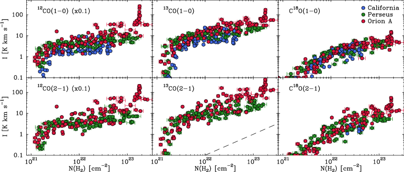
Figure 1: Velocity-integrated intensities of the $J$=1–0 (top) and $J$=2–1 (bottom) lines of the main CO isotopologs as a function of H₂ column density. The data are color-coded by cloud: blue circles for California, green for Perseus, and red for Orion A. The dashed line in the ¹³CO(2–1) panel indicates the slope of a linear trend. No $J$=2–1 data were taken for the California cloud apart from 13 C¹⁸O spectra from high column density positions. The lowest value of the intensity scale (0.1 K km s^-1) approximately corresponds to the line detection limit.

We started our analysis by comparing the emission of the different CO isotopologs in our three target clouds. Figure 1 presents velocity-integrated intensities for the $J$=1–0 and $J$=2–1 transitions of ¹²CO, ¹³CO, and C¹⁸O as a function of H₂ column density (no $J$=2–1 data were taken for the California cloud apart from a small number of C¹⁸O spectra). As the plots show, the intensity of each transition correlates significantly with $N$(H₂) over the approximately two orders of magnitude spanned by this parameter (approximately from 10²¹ to 10²³ cm^-2). Since each observed position was selected randomly among all cloud positions in the same column density bin, the correlation indicates that in each cloud, the value of $N$(H₂) is by itself a good predictor of the CO line intensity irrespective of the spatial location of the position. As discussed in Paper I, our correlations between ¹²CO(1–0) and ¹³CO(1–0) intensities with $N$(H₂) in Perseus match well the correlations between the same parameters derived from the full maps of Ridge et al. (2006). For the Orion A cloud, Yun et al. (2021) have recently presented intensity correlations for ¹³CO(1–0), C¹⁸O(1–0), and several dense-gas tracers, all based on full maps of the cloud. As shown with detail in Appendix C, these full-map correlations match well the results from our sampling observations, reinforcing the idea that the correlations are not an artifact of the sampling technique, but a common property of the clouds.

The plots in Fig. 1 also show that the correlation between the different intensities and the H₂ column density is similar in the three clouds, with the caveat that California spans a narrower range of $N$(H₂) than Perseus and Orion A. There are indeed noticeable differences between the clouds, and they are further discussed below, but the impression from the panels of Fig. 1 is that the main trends in the intensity versus $N$(H₂) correlation are common to the three clouds. In all three clouds, for example, the intensities of the ¹²CO and ¹³CO lines drop abruptly below an $N$(H₂) of about $2\times 10^{21}$ cm^-2, which corresponds to $A_{\mathrm{V}}\sim 2$ mag. (A similar drop may occur in C¹⁸O but is not noticeable due to the lower signal to noise of the lines.) This sharp drop likely results from the photodissociation of the CO molecules by the interstellar radiation field in the cloud outer layers, as modeled in Paper I for the case of Perseus. A similar drop has been observed in other clouds, like Taurus (Pineda et al., 2008), and is predicted by photodissociation models (van Dishoeck & Black, 1988; Wolfire et al., 2010).

Interior to the photodissociation boundary, the intensity of the ¹²CO(1–0) and ¹³CO(1–0) lines has a flatter-than-linear dependence on $N$(H₂), an effect that likely results from the combined high optical depth and thermalization of these lines. For the thinner C¹⁸O lines, the flattening at $N(\mathrm{H}_{2})>10^{22}$ cm^-2 likely results from the freeze-out of the CO molecules at the high densities characteristic of the high N(H₂), as discussed in detail in Paper I for the case of Perseus.

3.2 Temperature effects and temperature-corrected CO intensities

In addition to similarities, Fig. 1 shows systematic differences between the distribution of the CO intensity in the different clouds. The most noticeable one is the enhanced scatter and slightly steeper slope of the Orion A data at high column densities, an effect that is especially prominent in the J=2–1 lines of ¹²CO and ¹³CO. Since CO is thermalized and therefore sensitive to temperature, it is tempting to attribute the observed differences in the CO emission to differences in the distribution of the gas temperature across each cloud. These differences are known to exist in Orion A (e.g., Nagahama et al. 1998; Nishimura et al. 2015; Friesen et al. 2017), and they are likely larger than in California and Perseus due to its higher star-formation rate (Lada et al., 2010). To further investigate the effect of temperature variations in the CO emission, we needed to first estimate the gas temperature at each cloud position. In Paper I we used the C¹⁸O(2–1)/C¹⁸O(1–0) ratio to estimate a relatively constant gas temperature of around 11 K in Perseus, and a similar method can be used to estimate the temperature in Orion A. For California, however, our C¹⁸O(2–1) observations only covered a minority of the cloud positions due to time constraints, so we could not use the C¹⁸O line ratio to derive the temperature across the cloud. As an alternative, we explored several other methods for determining the gas temperature using data available for the three clouds. These methods include using the peak intensity of the optically thick ¹²CO(1–0) line, using the HCN/HNC ratio as recently proposed by Hacar et al. (2020), and using an empirical scaled-version of the dust temperature that has been calibrated to match the C¹⁸O line ratio predictions for the positions where it is available. Appendix D.1 describes the details of each method an evaluates its quality comparing the results with those of the C¹⁸O(2–1)/C¹⁸O(1–0) line ratio, which we consider the best available temperature indicator. As can be seen there, the dust temperature method supplemented with the NH₃-derived temperature estimates for the central part of Orion A from Friesen et al. (2017) provides the best results, and for this reason, it is the method of choice for carrying out the temperature corrections described below.

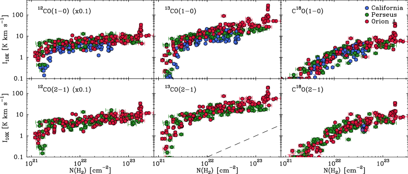
Figure 2: Temperature-corrected intensities of the $J$=1–0 (top) and $J$=2–1 (bottom) lines of the main CO isotopologs as a function of H₂ column density in California, Perseus, and Orion A (blue, green, and red circles, respectively). Note the lower level of scatter and the better inter-cloud agreement compared to the uncorrected intensities shown in Fig. 1. The dashed line in the ¹³CO(2–1) panel indicates the slope of a linear trend.

Once we had an estimate of the gas temperature at each cloud position, we used its value to correct the different line intensities for temperature variations across the cloud. Calculating a temperature correction factor for each position required determining how the intensity of the emerging lines change as a function of temperature, which is a nontrivial problem given the complex dependence of the intensity on multiple physical parameters. After exploring several options, we found that the best solution was to use a radiative transfer model, like the one presented in Paper I, and to predict the dependence of the different line intensities on temperature under realistic cloud conditions. A full description of the method is presented in Appendix D.2, while here we summarize its most relevant aspects. The Perseus model presented in Paper I assumes isothermal gas at 11 K and a simple parameterization of the physical and chemical structure of the cloud, and is able to reproduce simultaneously the emission from the different observed lines. To use this model to determine how the intensity of the different lines varies as a function of the gas temperature, we reran it using a grid of temperatures that ranges from 8 K to 100 K. Dividing each model intensity by the intensity obtained at a reference temperature of 10 K, we derived a series of correction factors $f_{10\mathrm{K}}(T_{\mathrm{k}})$. Using these correction factors, we can convert any observed intensity into the expected intensity that the gas would emit if it were at 10 K. We define this “corrected” intensity as

$$I_{10\mathrm{K}}\equiv\frac{I}{f_{10\mathrm{K}}(T_{\mathrm{k}})},$$ (1)

where $I$ is the observed intensity and $f_{10\mathrm{K}}(T_{\mathrm{k}})$ is the model correction factor. Values for these factors for each transition observed in our survey are presented in Tables 10 and 11.

Using the above factors, we converted the intensities of the CO isotopologs into their expected values for gas at 10 K, and present the results as a function of $N$(H₂) in Fig. 2. Compared to the uncorrected intensities, the Orion A corrected intensities show a significant decrease of dispersion, which is a factor of 1.6 for the main isotopologs. As a result, the rms dispersion of the Orion A CO intensities is typically 0.2 dex, which is similar to the rms estimated for Perseus and California. These two clouds have also been temperature corrected, but the effect of the correction is minimal due to the clouds almost-constant temperature.

In addition to decreasing the dispersion, the temperature correction helps equalize the line intensities of the three clouds. For all transitions, the temperature-corrected intensities of Perseus and Orion A are practically indistinguishable, apart from the spike of points near $2\times 10^{23}$ cm^-2 in Orion A caused by the wings of the Orion Kleinmann–Low (Orion-KL) outflow. The line intensities of the California cloud are also close to those of Perseus and Orion A, although they cluster at the lower end of the range spanned by the other two clouds. This equalization of the temperature-corrected intensities strongly suggests that most differences seen between the uncorrected intensities are due to differences in the gas temperature, and that once the temperature has been equalized (even using an approximate method like ours) a common pattern of emission emerges from the data. The existence of this common emission pattern indicates that after H₂ column density, the gas kinetic temperature is the next physical parameter that controls the intensity of the CO lines, and that when it is adjusted, the intensity of the CO isotopolog lines lines can be predicted for each $N$(H₂) value with a precision close to 0.2 dex.

The only peculiar emission feature in Fig. 2 that remains unaffected by the temperature correction is the sudden increase in the intensity of the Orion A lines at column densities close to $2\times 10^{23}$ cm^-2. As mentioned before, this intensity increase is associated with the Orion-KL molecular outflow, and is accompanied by the appearance of prominent high velocity wings in the CO spectra. For the optically thick CO lines, the appearance of the wings increases the velocity range available for the CO emission to escape, and this effect contributes to the large increase seen in intensity. The intensity increase, however, can also be seen in the optically thin C¹⁸O emission, so it must be accompanied by a local increase in the CO abundance that likely results from the action of outflow shocks and dust heating caused by the feedback of the massive stars in Orion-KL. The very extended N₂H⁺ emission seen toward the ISF (Hacar et al., 2018) indicates the presence of large-scale CO freeze-out, and this process is likely being reversed in the vicinity of Orion-KL by the action of the stellar feedback. While smaller abundance enhancements occur toward individual low mass stars (such as the L1448 region in Perseus), the extreme effect of the Orion-KL outflow is unique to the Orion A cloud, and seems to represent a different regime of chemical abundance driven by high-mass star formation. This regime coincides with the small fraction of gas having column densities higher than of $2\;10^{23}$ cm^-2, which corresponds to a mass density of 0.94 g cm^-2, a value practically equal to the 1 g cm^-2 threshold for star formation proposed by Krumholz & McKee (2008). This different chemical regime is therefore likely to occur in other regions of high-mass formation, although further observations are required to reach a firm conclusion.

3.3 Quantifying the intensity comparison

So far, our comparison of the intensity profiles in the different clouds has been purely qualitative. To quantify it, we need a statistical tool that tests whether two distributions of points are equal. A convenient choice for this is the test proposed by Fasano & Franceschini (1987, the FF test hereafter), which generalizes the classical Kolmogorov-Smirnov test to multidimensional distributions of data. As the Kolmogorov-Smirnov test, the FF test determines the probability (p-value) that any two 2D samples arise from the same underlying distribution. To apply the test, it is customary to choose a threshold probability $\alpha$ (typically 0.05) so that if the p-value is lower than $\alpha$, the hypothesis that the two samples arise from the same distribution (the null hypothesis) can be considered as rejected. As often stressed in the literature (e.g., Press et al. 1992), p-values larger than $\alpha$ do not guarantee that the two samples arise from exactly the same distribution, but that they are not different enough to reach a definitive conclusion. Given this caveat, and the arbitrary choice of the threshold value $\alpha$, our use of the FF test does not pretend to prove or disprove mathematically that any two intensity distributions are completely equivalent, but to explore how significant any differences may be.

Table 1: FF test p-values for a comparison between the emission of the different CO isotopologs in each pair of clouds.

No temperature correction
Clouds	CO(1–0)	13CO(1–0)	C18O(1–0)	CO(2–1)	13CO(2–1)	C18O(2–1)
California - Perseus	$4.9\;10^{-9}$	$4.8\;10^{-6}$	$5.2\;10^{-1}$	–	–	–
California - Orion A	$7.8\;10^{-10}$	$2.9\;10^{-9}$	$9.4\;10^{-2}$	–	–	–
Perseus - Orion A	$2.8\;10^{-2}$	$1.7\;10^{-2}$	$2.2\ 10^{-1}$	$4.7\;10^{-3}$	$3.9\;10^{-3}$	$8.6\;10^{-2}$
With temperature correction
Clouds	CO(1–0)	13CO(1–0)	C18O(1–0)	CO(2–1)	13CO(2–1)	C18O(2–1)
California - Perseus	$2.5\;10^{-6}$	$5.0\;10^{-6}$	$5.2\;10^{-1}$	–	–	–
California - Orion A	$8.4\;10^{-9}$	$2.0\;10^{-5}$	$9.7\;10^{-2}$	–	–	–
Perseus - Orion A	$4.9\;10^{-1}$	$2.1\;10^{-2}$	$3.1\ 10^{-1}$	$6.7\;10^{-1}$	$4.4\;10^{-2}$	$3.0\;10^{-1}$

To apply the FF test to our data, we used its implementation in the R statistical program (R Core Team, 2018) as presented by Puritz et al. (2021), which provides a fast and straightforward evaluation of the test p-value. Since the FF test compares distributions in pairs, we applied the test to each pair of clouds and to each CO transition observed in both clouds. To avoid any bias caused by the different $N$(H₂) extent of the different clouds, we restricted the comparison between clouds to the intensity values inside a common range of $N$(H₂), which for comparisons involving the California cloud is $2\times 10^{21}$-$4.8\times 10^{22}$ cm^-2, and for comparisons between Perseus and Orion A is $2\times 10^{21}$-$1.5\times 10^{23}$ cm^-2. Finally, to study the effect of the temperature correction, we ran the FF test before and after applying the correction.

Table $a$ summarizes the p-values derived from the FF test for each cloud pair and transition for which data are available. Values in bold face indicate probabilities that exceed the standard 0.05 threshold value and are therefore consistent with the two intensity distributions being equivalent. As can be seen, each pair comparison involving a C¹⁸O transition exceeds the 0.05 threshold irrespectively of whether the temperature correction has been applied or not, although the temperature-corrected p-values are slightly larger and therefore suggest a better match. This low sensitivity of the FF test to the temperature correction results from the small value of the correction for the optically thin C¹⁸O lines (Fig. 17), and has the advantage of making the C¹⁸O line comparison almost independent of the temperature estimate. Since the C¹⁸O emission is optically thin, the similarity between the intensity distributions of the three clouds suggests that the clouds share a similar CO abundance distribution.

Another conclusion that can be derived from the data in Table $a$ is that, in contrast with the C¹⁸O results, the comparison of the CO and ¹³CO emission from California with both Perseus and Orion A returns p-values significantly lower than the 0.05 threshold irrespectively of the use of the temperature correction. If we interpret the C¹⁸O comparison as indicative that the three clouds have similar CO abundance profiles, the low p-values of the CO and ¹³CO comparison suggest that either the excitation or the optical depth in California is different from that in Perseus and Orion A. Figure 2 suggests that the CO and ¹³CO intensities in California are lower than in Perseus and Orion A, and an experiment of multiplying the California intensities by a factor of 1.5 brings the clouds in better agreement. This result suggests that we are either overcorrecting the California intensities or that the California intensities are intrinsically lower due to optical depth effects, such as self-absorptions caused by the narrower lines. Further observations of these isotopologs are needed to reach a firm conclusion.

Finally, the p-values in Table $a$ confirm the success of the temperature correction equalizing the intensity of the main CO isotopolog in Perseus and Orion A. Before applying a temperature correction, the FF test for both CO(1–0) and CO(2–1) returns p-values below the 0.05 threshold, while the p-values after applying the temperature correction increase to 0.49 and 0.67 for $J$=1–0 and 2–1, respectively. This large change in the p-value reflects the large size of the temperature correction for the very optically thick lines of the main isotopolog, and illustrates the need of considering temperature variations when comparing the CO emission from different clouds.

Somewhat surprisingly, the temperature correction does not bring the p-value of the ¹³CO intensities over the 0.05 threshold, although it increases the p-value of the 2–1 transition by one order of magnitude. The reason for this failure may represent an intrinsic difference between the clouds, possibly caused by different isotopic fractionation (Langer et al., 1980; Ishii et al., 2019), or simply represent a failure of our temperature correction caused by an underestimate of the ¹³CO optical depth.

To summarize, our analysis shows that the FF test is a useful tool for quantitatively comparing the distribution of intensities between clouds. When applied to the C¹⁸O emission, the FF test shows that the emission from the three clouds is statistically indistinguishable, and since this emission is optically thin, it likely indicates that the clouds have similar CO abundance distributions. The observed differences between the distributions of the optically thick ¹²CO and ¹³CO emissions likely arise from differences in the internal temperature structure of the clouds.

3.4 Traditional dense-gas tracers

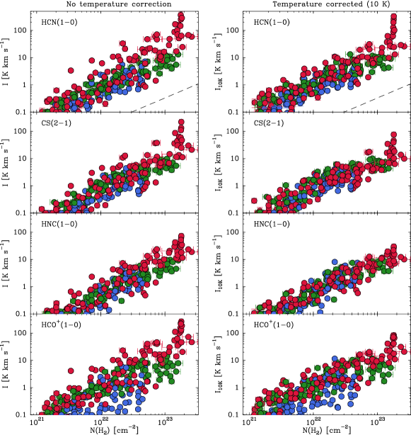
Figure 3: Velocity-integrated intensities of the traditional dense-gas tracers HCN(1–0), CS(2–1), HNC(1–0), and HCO⁺(1–0) as a function of H₂ column density. Left panels: Original uncorrected data. Right panels: Data after applying the correction factors described in Appendix D.2 to simulate emission at a constant temperature of 10 K. Note the decrease in dispersion and the better agreement between clouds after the temperature correction. The data are color-coded as in previous figures: blue for California, green for Perseus, and red for Orion A. The dashed line in the top panels represents a linear trend for comparison.

We now turn our attention to several molecular species that combine a high dipole moment with bright 3 mm wavelength lines: HCN, CS, HCO⁺, and HNC. Following Paper I, we collectively refer to these species as “traditional dense-gas tracers” since they have been used in the past as indicators of high-density gas in molecular clouds (e.g., Evans 1999). Recent research shows that these tracers are less selective of dense material than initially thought (Kauffmann et al., 2017; Pety et al., 2017; Watanabe et al., 2017; Shimajiri et al., 2017; Evans et al., 2020; Tafalla et al., 2021; Dame & Lada, 2023), although they are still widely used by the extragalactic community due to their bright emission lines (Gao & Solomon, 2004; Usero et al., 2015; Gallagher et al., 2018; Jiménez-Donaire et al., 2019)

Since the traditional dense-gas tracers combine a large abundance and a high dipole moment, their low-$J$ lines are expected to be optically thick over a significant fraction of any cloud. For our selected lines, this expectation is confirmed by the value of the intensity ratio between the main and a rare isotopolog (H¹³CN, C³⁴S, H¹³CO⁺, and HN¹³C). As shown in Fig. 19, all these ratios systematically lie below the expected abundance ratio by a large margin, indicating that the main isotopolog lines must be highly saturated over most of the cloud positions.

As it happened with CO, the high optical depth of the traditional dense-gas tracer lines makes their emission potentially sensitive to temperature variations. To evaluate this effect, we present in Fig. 3 plots of the integrated intensity of HCN(1–0), CS(2–1), HNC(1–0), and HCO⁺(1–0) as a function of H₂ column density for two cases: uncorrected data (left panels) and data corrected for temperature variations using the factors described in Appendix D.2 (right panels). As can be seen, the temperature-corrected data present a lower degree of scatter and a better agreement between the emission from the three clouds compared to the uncorrected data. We interpreted this equalizing effect of the temperature correction as an indication that most of the inter and intra cloud differences in the emission seen in the uncorrected data arise from variations in the gas kinetic temperature. An exception to this equalizing effect are the large increases in the HCN(1–0) and CS(2–1) intensity at column densities around $2\times 10^{23}$ cm^-2 in the Orion A cloud. As we will see the next section using the more abundance-sensitive rare isotopologs, these intensity increases are likely the result of abundance enhancements caused by high-mass star-formation feedback.

Since our goal was to investigate how the molecular emission is generated inside the clouds, we focused on the temperature-corrected data and searched for additional features in the intensity profiles. A first feature to notice is the tight correlation between the intensity of all traditional dense-gas tracers and the H₂ column density. The correlation is stronger in HCN(1–0), CS(2–1), and HNC(1–0), and is characterized by values of the Pearson’s $r$ coefficient in the range of 0.87-0.90 (Table 2). The HCO⁺(1–0) intensities, on the other hand, present a significantly higher degree of scatter, which is mostly caused by the California data lying significantly below the Orion A and Perseus data. The Pearson’s $r$ coefficient is 0.80, which still indicates a strong level of correlation between the HCO⁺ emission and the H₂ column density. Paper I already noted that the HCO⁺(1–0) intensities in Perseus presented a higher degree of scatter than the other lines, and the new California data show an even larger dispersion. As shown in the next section, the intensity of the H¹³CO⁺ rare isotopolog presents little scatter and a tight correlation with $N$(H₂), suggesting that the larger scatter of the main isotopolog lines results from optical depth effects. An inspection of high velocity resolution HCO⁺(1–0) spectra taken toward selected positions reveals the presence of significant self-absorption features in some spectra that artificially truncate the emission and therefore lower the intensity.

Table 2: Statistics of the (logarithmic) correlation between the temperature-corrected intensity of traditional dense-gas tracers and H₂ column density.

Transition	$r$-Pearson	Slope
HCN(1–0)	0.87	$1.12\pm 0.04$
CS(2–1)	0.88	$1.07\pm 0.03$
HCO+(1–0)	0.80	$0.97\pm 0.04$
HNC(1–0)	0.90	$1.16\pm 0.03$

Table 3: FF p-values for traditional dense-gas tracers.

No temperature correction
Clouds	HCN(1-0)	CS(2-1)	HNC(1-0)	HCO+(1-0)
Cal-Pers	$2.3\;10^{-2}$	$3.7\;10^{-2}$	$7.2\;10^{-2}$	$1.0\;10^{-6}$
Cal-Ori	$4.1\;10^{-2}$	$1.1\;10^{-1}$	$1.7\;10^{-2}$	$2.2\;10^{-4}$
Pers-Ori	$3.0\;10^{-2}$	$3.5\;10^{-1}$	$2.5\;10^{-1}$	$3.0\;10^{-2}$
With temperature correction
Clouds	HCN(1-0)	CS(2-1)	HNC(1-0)	HCO+(1-0)
Cal-Pers	$1.4\;10^{-1}$	$2.8\;10^{-2}$	$1.7\;10^{-2}$	$7.2\;10^{-5}$
Cal-Ori	$3.7\;10^{-2}$	$2.7\;10^{-1}$	$1.9\;10^{-2}$	$1.9\;10^{-5}$
Pers-Ori	$2.8\;10^{-1}$	$5.9\;10^{-2}$	$5.1\;10^{-1}$	$3.3\;10^{-1}$

In addition to a strong correlation with $N$(H₂), Fig. 3 shows that the temperature-corrected intensity of the traditional dense-gas tracers has an approximately linear dependence on column density (indicated by the dashed lines in the top panels). The only significant deviation from this trend occurs near $N$(H₂) = $2\times 10^{23}$ cm^-2, where several tracers present a sudden intensity increase coincident with the position of the Orion Nebula Cluster (ONC) and the Orion-KL outflow. The origin of this increase seems to be a combination of abundance variations in some species and a drop in the optical depth due to the wide outflow wings caused by the outflow (as seen in the isotopic ratios of Fig 19). In the next section we use the intensity distribution of the rare isotopologs to disentangle these two contributions. For the current analysis, we focused on the slope of the distribution as determined from a least squares fit to the combined data of the three clouds (including the anomalously bright positions at high column densities). The fit results, summarized in the third column of Table 2, show that the slopes lie in a narrow range (0.97-1.16) and are therefore very close to unity, as expected from the inspection of Fig. 3. This quasi-linear slope can be followed without significant changes until the emission reaches the detection limit ($\approx 0.1$ K km s^-1), indicating the absence of breaks until the H₂ column density reaches its lowest values ($\approx 10^{21}$ cm^-2). The radiative transfer model presented in Paper I showed that the gas volume density approximately follows the column density (Sect. 5.1), so the continuity of the slope in $N$(H₂) indicates that there is no particular density at which the emission of the traditional dense-gas tracers suddenly changes behavior or disappears. Because of this, we can say that the tracers are sensitive to the gas density (since their intensity gradually increases with this parameter), but that they are not selective of any density value, since the emission depends continuously on this parameter. In addition, molecular clouds present probability distribution functions of column density that increase nonlinearly toward low column densities (Lombardi et al., 2015). As a result, the cloud-integrated intensity of any traditional high-density tracer is expected to be dominated by the contribution of the cloud low-density regions, as previously shown by different authors (Kauffmann et al., 2017; Pety et al., 2017; Watanabe et al., 2017; Shimajiri et al., 2017; Evans et al., 2020; Tafalla et al., 2021; Jones et al., 2023).

To finish our analysis, we again used the FF test to quantify the similarities between the emission distributions in the three clouds. Table 3 presents the p-values derived using the FF test for both cases of no temperature correction and temperature correction. In agreement with the expectation from Fig. 3, using temperature correction improves the agreement between the clouds, reinforcing the idea that despite its simplicity, the correction partially compensates for differences in the gas temperature between the clouds. The better agreement of the temperature-corrected intensities also suggests that there are important similarities between the emission of the three clouds. The largest differences occur again when comparing California with Perseus and Orion A, especially for the case of HCO⁺(1–0). For the other lines, the FF test produces a mix of p-values slightly larger or smaller than the 0.05 threshold, confirming that there are noticeable similarities between the emission of the clouds, but not necessarily to the point of making them indistinguishable. In contrast with the peculiar behavior of the California cloud, a comparison between the intensity-corrected intensities in Perseus and Orion A produces p-values that are always larger than the 0.05 threshold for the four observed lines (although only marginally for CS(2–1)). The emission of Perseus and Orion A therefore appears indistinguishable when comparing positions in their common range of H₂ column density.

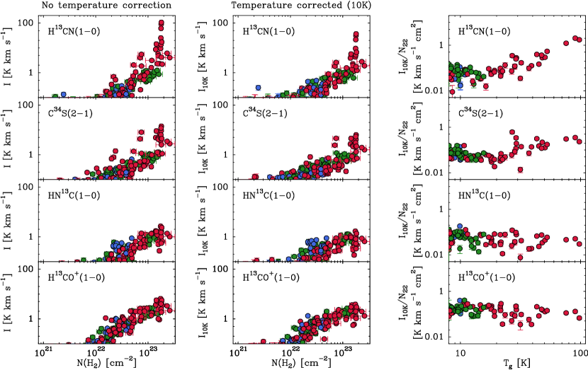
Figure 4: Intensity distributions of the rare isotopologs of the traditional dense-gas tracers represented in Fig. 3. Left panels: Original uncorrected data. Middle panels: Data after applying the correction factors described in Appendix D.2 to simulate emission at a constant temperature of 10 K. Right panels: Ratio between the temperature-corrected intensity and the H₂ column density (in units of $10^{22}$ cm^-2) as a function of gas temperature. All data are color-coded as in previous figures.

3.5 Rare isotopologs of the traditional dense-gas tracers

The lines of the traditional dense-gas tracers discussed in the previous section are optically thick and therefore relatively insensitive to possible abundance variations. To investigate these variations, we had to rely on less abundant isotopologs, such as H¹³CN, C³⁴S, HN¹³C, and H¹³CO⁺, whose lines are likely to be optically thin as suggested by the relative intensities of the hyperfine components of H¹³CN(1–0).

Figure 4 presents the intensity distribution of the most abundant rare isotopologs of the traditional dense-gas tracers studied in the previous section. The left and middle panels show their emission as a function of H₂ column density both using uncorrected intensities (left panels) and intensities corrected for temperature variations using the prescriptions detailed in Appendix D.2 (middle panels).

As can be seen, the rare-isotopolog lines are weaker than the main-species lines by about one order of magnitude, and as a result, their detection in our survey is limited to H₂ column densities larger than approximately $10^{22}$ cm^-2. In this range of detection, the intensity of most species is very similar in the three clouds. For H¹³CO⁺(1–0), this is in contrast with the behavior of the main isotopolog, which as we saw in Fig. 3, presents strong excursions toward low intensities in California. The lack of similar excursions in the H¹³CO⁺(1–0) intensity supports the interpretation that HCO⁺(1–0) suffers from optical depth effects, most likely from the strong self-absorptions known to affect the narrower California lines.

If we compare the left and middle panels of Fig. 4, we notice that applying the temperature correction decreases some of the intensity excursions seen in H¹³CN(1–0) and C³⁴S(2–1), but has otherwise little effect on the data. This is due to the small value of the correction, which is typically less than a factor of 2 (Fig. 17), and as a result, it cannot remove the strong intensity increase seen in H¹³CN(1–0) and C³⁴S(2–1) toward $N(\mathrm{H}_{2})\approx 2\times 10^{23}$ cm^-2.

To investigate the intensity increase of H¹³CN(1–0) and C³⁴S(2–1) in Orion A, the right panels of Fig. 4 present plots of the ratio between the temperature-corrected intensity and the H₂ column density as a function of the gas kinetic temperature for the four rare isotopologs. Positions with gas temperature below 20 K are present in all three clouds, while all warmer positions are located in the ISF of Orion A, especially in the vicinity of Orion KL and the ONC. As can be seen, the ratios for HN¹³C and H¹³CO⁺ (bottom panels) remain approximately constant, with a possible slight decrease at intermediate temperatures, despite a factor of 10 variation in the gas temperature. On the other hand, the ratios for H¹³CN and C³⁴S (top panels), present significant correlations with the gas temperature for values larger than approximately 20 K. In the 20-100 K temperature range, the ratio for H¹³CN increases by about one order of magnitude while the ratio for C³⁴S increases about a factor of 5.

Since the correlations seen in the right panels of Fig. 4 involve intensities already corrected for temperature variations, their most likely origin must be differences in the abundance of the species as a function of the gas temperature. If this is case, the approximately constant intensity/column density ratios of H¹³CO⁺ and HN¹³C suggest that these two species are relatively immune to temperature-related abundance variations, which makes them stable tracers of the column density. The increase in the intensity/column density ratios of H¹³CN and C³⁴S, on the other hand, strongly indicates that the abundance of these two species depends sensitively on temperature once this parameter exceeds a threshold value of around 20 K. The larger increase of the H¹³CN intensity/column density ratio indicates that this species is more sensitive to temperature than C³⁴S, and that its abundance is expected to vary as a result of gas temperature increases caused by the action of star formation.

Our finding of an HCN abundance enhancement at high temperatures is in good agreement with previous research on the chemistry of Orion A, which has found a significant increase of the HCN/HNC ratio with the gas kinetic temperature (Goldsmith et al., 1981; Schilke et al., 1992; Hacar et al., 2020). Although not fully understood, this increase likely results from the activation of temperature-sensitive neutral-neutral reactions that alter the total abundance of the two species and their abundance ratio (Herbst et al., 2000; Graninger et al., 2014). Less work has been carried out on the possible temperature dependence of the abundance of CS. We note however that most positions with high CS abundance in Orion A present evidence for high-velocity wings caused by the Orion-KL outflow, and that chemical surveys of bipolar outflow gas often show significant abundance enhancements of both HCN and CS (but little or no enhancement of HNC and HCO⁺; see Bachiller & Pérez Gutiérrez 1997, Tafalla et al. 2010, and Lefloch et al. 2021). Clearly more work is needed to understand the different contributions to the abundance behavior of HCN, CS, HNC, and HCO⁺ at high temperatures. For the purposes of our study, our main conclusion is that the temperature enhancement resulting from star-formation feedback introduces a new chemical regime in the cloud gas that seems to coincide with the onset of high-mass star formation.

Table 4: FF p-values for isotopologs of traditional dense-gas tracers.

No temperature correction
Clouds	H13CN(1-0)	C34S(2-1)	HN13C(1-0)	H13CO+(1-0)
Cal-Pers	$6.3\;10^{-1}$	$4.1\;10^{-1}$	$1.5\;10^{-1}$	$8.3\;10^{-1}$
Cal-Ori	$5.3\;10^{-1}$	$4.0\;10^{-1}$	$4.3\;10^{-2}$	$8.0\;10^{-1}$
Pers-Ori	$3.3\;10^{-1}$	$4.6\;10^{-1}$	$6.6\;10^{-1}$	$3.3\;10^{-1}$
With temperature correction
Clouds	H13CN(1-0)	C34S(2-1)	HN13C(1-0)	H13CO+(1-0)
Cal-Pers	$3.1\;10^{-1}$	$4.5\;10^{-1}$	$1.2\;10^{-1}$	$4.8\;10^{-1}$
Cal-Ori	$1.1\;10^{-1}$	$7.3\;10^{-1}$	$2.7\;10^{-3}$	$3.6\;10^{-1}$
Pers-Ori	$2.2\;10^{-1}$	$4.3\;10^{-2}$	$4.1\;10^{-1}$	$3.4\;10^{-1}$

To conclude our analysis of the rare isotopologs, we present in Table 4 the results of the FF test for all combinations of the lines and pairs of clouds, both before and after applying the temperature correction. Since the isotopologs are not detected at H₂ column densities lower than about $10^{22}$ cm^-2, only values larger than this threshold have been considered. As in previous FF tests, the California data have been compared with Perseus and Orion A data having column densities smaller or equal to $4.8\times 10^{22}$ cm^-2, and the Perseus data have been compared with Orion A data up to a column density of $1.5\times 10^{23}$ cm^-2. As can be seen in the table, all p-values for the uncorrected comparison exceed the 0.05 threshold except for the comparison of HN¹³C(1–0) between California and Orion A, which returns a value of 0.04. After applying the temperature correction, most p-values remain larger than the 0.05 threshold, except for the already mentioned HN¹³C(1–0) and the comparison of C³⁴S(2–1) between Perseus and Orion, whose p-value drops by one order of magnitude with respect to the uncorrected comparison. This drop seems anti-intuitive in view of the plots of Fig. 4, and seems to occur because the temperature correction decreases the dispersion of the data, so any slight difference between the emission of the clouds becomes more significant. Still, the fact that the majority of p-values exceed the 0.05 threshold is an indication that while small differences may exist, the emission from the three clouds presents strong similarities when similar column densities are compared. The main differences between the clouds seem therefore to arise from the fact that they reach very different peak column densities.

3.6 N₂H⁺ and the onset of molecular freeze-out

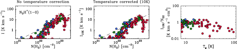
Figure 5: Distributions of N₂H⁺(1–0) integrated intensity. Left panel: Original uncorrected data. Middle panel: Data after applying the correction factors described in Appendix D.2 to simulate emission at a constant temperature of 10 K. Right panel: Ratio between the temperature-corrected intensity and the H₂ column density (in units of $10^{22}$ cm^-2) as a function of gas temperature. All data are color-coded as in previous figures.

In contrast with the traditional dense-gas tracers, which freeze out onto the cold dust grains at high densities and low temperatures, N₂H⁺ remains in the gas phase and its abundance is enhanced at high densities, likely as a result of the freezing out of CO (Kuiper et al., 1996; Caselli et al., 1999; Aikawa et al., 2001; Tafalla et al., 2002; Lee et al., 2004). Since N₂H⁺ also has a high dipole moment (Havenith et al., 1990), it has become a tracer of choice for identifying the dense and cold condensations responsible for star formation in clouds (Bergin & Tafalla, 2007). To illustrate the behavior of the N₂H⁺ emission in the three clouds of our sample, we present its distribution in Fig. 5. As in previous figures, the left and middle panels show the distribution of intensity as a function of H₂ column density both without temperature correction and after applying the temperature correction factors described in Appendix D.2. Since the temperature correction for N₂H⁺ never exceeds a factor of 2 (Fig. 17), the two distributions in the figure look very similar.

As can be seen from Fig. 5, the distribution of N₂H⁺(1–0) intensity differs significantly from that of the traditional dense-gas tracers. It follows an almost linear correlation with $N$(H₂) at high column densities, but below $2\times 10^{22}$ cm^-2 it drops nonlinearly with column density, and remains undetected at values below $10^{22}$ cm^-2. This sudden change in the emission is unique to N₂H⁺(1–0), and makes this species a highly selective tracer of the dense gas in a cloud.

Table 5: FF test p-values for N₂H⁺(1–0).

Clouds	No $T_{\mathrm{k}}$ corr.	With $T_{\mathrm{k}}$ corr.
Cal-Pers	$8.8\;10^{-1}$	$6.1\;10^{-1}$
Cal-Ori	$3.7\;10^{-1}$	$2.0\;10^{-1}$
Pers-Ori	$3.1\;10^{-1}$	$2.1\;10^{-1}$

As Fig. 5 shows, the distribution of N₂H⁺(1–0) emission in the three clouds is very similar independently of whether a temperature correction has been applied or not. This good agreement is confirmed by the FF test results reported in Table 5, which show that the p-value in all comparisons exceeds the 0.05 threshold both with and without temperature correction. The good match between the clouds in the nonlinear region between $10^{22}$ and $2\times 10^{22}$ cm^-2 is especially remarkable because the nonlinear change is likely caused by the onset of CO freeze-out, a process that is also sensitive to volume density because the freeze-out time depends on the collision time between molecules and dust grains (Leger, 1983). The similar location of the N₂H⁺(1–0) change in the three clouds suggests that the critical density for CO freeze-out is reached at a similar column density in all of them despite their very different peak H₂ column densities and star-formation rates.

Also noticeable in the distribution of N₂H⁺(1–0) is the sharp drop toward the highest column densities reached in Orion A at about $10^{23}$ cm^-2 coinciding with the ONC and Orion BN/KL. This drop has been previously noticed by a number of authors, including Tatematsu et al. (2008), Kauffmann et al. (2017), Hacar et al. (2018), and Yun et al. (2021), and occurs at the same column densities at which HCN and CS present their abundance increase associated with the high-temperature gas. To investigate the effect of temperature in the N₂H⁺ abundance, we again calculated the ratio between the N₂H⁺ intensity and the H₂ column density, and present the result as a function of the gas temperature in the right panel of Fig. 5. To make this plot, we restricted the comparison to H₂ column densities larger than $2\;10^{22}$ cm^-2 since this is the approximate range at which the N₂H⁺ intensity depends quasi-linearly with $N$(H₂). As can be seen, the intensity-column density gradually decreases in gas hotter than about 30 K, and by 100 K, it has decreased by about one order of magnitude with respect to its low-temperature value.

Although the N₂H⁺ drop presents more scatter than the increases in H¹³CN and C³⁴S, the trend points again to a change in the gas chemical composition triggered by the feedback from star formation. A drop in the N₂H⁺ abundance is indeed expected as a result of the release of CO from the dust grains due to protostellar heating, and has been previously observed toward individual star-forming regions (Jørgensen, 2004; Caselli & Ceccarelli, 2012; Jørgensen et al., 2020). Observations of additional high-mass star-forming regions are necessary to confirm this interpretation.

3.7 Line luminosity estimates from sampling observations and comparison with mapping results

So far we have only used the sampling data to study the distribution of line intensities as a function of H₂ column density. This type of distribution represents the most immediate output from the sampling observations, and as we have seen, provides a detailed description of the emission properties from a cloud. The sampling data can also be used to estimate other emission properties, such as the line luminosity of a cloud, which corresponds to the integral of the line intensity over the cloud surface area. This luminosity can be calculated from the sampling data by adding the contribution from each column density bin to the product of the mean line intensity ($I_{n}$) times the surface area subtended by that bin ($A_{n}$). In other words,

$$L=\sum_{n=1}^{m}I_{n}\;A_{n},$$ (2)

where in our case $n$ runs from 1 to $m$= 8, 10, and 12 for California, Perseus, and Orion A, respectively.

In practice, the mean line intensity $I_{n}$ can be estimated by averaging all the spectra observed toward a given column density bin (ten positions in our survey) and integrating the emission over the full velocity range. The surface area $A_{n}$ subtended by the bin can be estimated from the available extinction maps (Lombardi et al., 2014; Zari et al., 2016; Lada et al., 2017) by counting the number of pixels belonging to the bin and multiplying the result by the pixel area assuming an appropriate cloud distance. Combining these two quantities, it is straightforward to use the sampling data to estimate the luminosity of any line emitted by a cloud.

To test whether the above method provides accurate estimates of the line luminosities, we searched the literature for line luminosity determinations based on the standard mapping technique in any of our three target clouds, and we calculated equivalent luminosity estimates using our sampling data. As expected, most available luminosity determinations involve CO transitions since this molecule has been the tracer of choice for large-scale mapping.

The most complete set of luminosity determinations that can be used to compare with our sampling estimates is that of Lewis et al. (2022), who have determined ¹²CO(1–0) luminosities for California, Perseus, and Orion A as part of their study of 12 nearby molecular clouds. These authors have used for their estimates data from the Milky Way survey of Dame et al. (2001), and while they do not explicitly provide the resulting luminosities, those can be trivially derived from the $\alpha_{\mathrm{CO}}$ conversion factors and the cloud masses presented in their Table 1. Due to the large scale of the maps used by Lewis et al. (2022) (see their Figs. 12 and 13), the resulting luminosities should be compared with sampling estimates using the full extent of the clouds.

Additional CO luminosities for the Orion A cloud have been presented by Nishimura et al. (2015), who have estimated values for both the $J$=1–0 and 2–1 transitions of ¹²CO, ¹³CO, and C¹⁸O. These luminosities, however, have been estimated after applying to the data a noise-reduction mask that assigns “zero values at the emission free pixels” (their Sect. 2.1), and as a result, this set of luminosity estimates neglects the contribution from the outer parts of the cloud, which according to our sampling estimates is significant. To properly compare luminosities estimated using sampling with the results from Nishimura et al. (2015), it is therefore critical to exclude the fraction of the cloud that these authors have masked out. This information is only available for the $J$=2–1 lines, whose (masked) maps are publicly available (Sect. 6 in Nishimura et al. 2015), so our comparison with the sampling method has to be restricted to the $J$=2–1 transitions. For them, we downloaded the maps from the repository, verified the luminosity values given by Nishimura et al. 2015 in their Table 1, and estimated the amount of surface area in each of our column density bins that was left unmasked. Using these values, we used Eq. 2 to derive sampling-based luminosities that can be properly compared with the values presented by Nishimura et al. (2015).

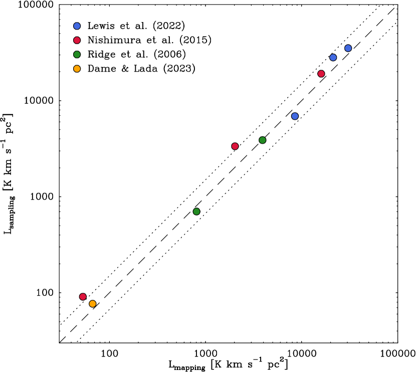
Figure 6: Comparison between line-luminosity estimates based on mapping data from the literature and equivalent estimates using sampling observations. The blue circles represent CO(1–0) luminosities of California, Perseus, and Orion A from Lewis et al. (2022), the red circles the CO(2–1), ¹³CO(2–1), and C¹⁸O(2–1) luminosities of Orion A from from Nishimura et al. (2015), the green circles the CO(1–0) and ¹³CO(1–0) luminosities of Perseus from Ridge et al. (2006), and the yellow circle the HCN(1–0) luminosity of Perseus from Dame & Lada (2023). The dashed line marks the locus of equal estimates, and the dotted lines correspond to differences of 50%. All estimates assume the cloud distances given in Sect. 1.

A final set of CO luminosities based on mapping observations can be derived from the publicly available maps of the Coordinated Molecular Probe Line Extinction and Thermal Emission (COMPLETE) survey of Perseus presented by Ridge et al. 2006 These ¹²CO(1–0) and ¹³CO(1–0) maps contain more than $10^{5}$ pixels each, and we spatially integrated them to estimate cloud luminosities. Since the COMPLETE survey did not cover the full extent of the Perseus cloud (see the coverage in Fig. 2 of Ridge et al. 2006), we estimated the amount of area of each bin covered by the COMPLETE maps and used these values to calculate equivalent sampling-based estimates.

Apart from CO, the only species whose line luminosity has been estimated in any of our three target clouds is HCN. Dame & Lada (2023) have recently presented an estimate of the HCN(1–0) luminosity from Perseus using a map made with the Center for Astrophysics (CfA) 1.2 m telescope that attempts to cover the full extent of the cloud emission. While this map only extends to a column density equivalent to our second bin (based on its CO cutoff), these authors have used their larger CO map to estimate the contribution from the remaining ”weak, unobserved HCN,” so we used this corrected luminosity to compare with out sampling estimate for the full cloud.

Fig. 6 summarizes the comparison between the mapping and sampling luminosity estimates by representing one quantity against the other (numerical values are given in Table 12). The diagonal dashed line indicates the locus of equal luminosity estimates, and the parallel dotted lines delimit the region where the mapping and sampling estimates agree at the 50% level. As can be seen, the luminosity estimates span almost three orders of magnitude and systematically cluster along the equal-value dashed line, indicating an overall good agreement between the two methods used to estimate luminosities.

As the figure indicates, the level of agreement between the mapping and sampling estimates seems to slightly vary between the different data sets, although there is no evidence for significant variations with the choice of cloud or tracer. The Lewis et al. (2022) estimates (blue circles), which are the only ones that include simultaneously our three target clouds, present differences with the mapping results that are only at the level of 30% or less. This is despite the use of of very different telescopes: the beam solid angle of the CfA 1.2m telescope is 625 times larger than that of the IRAM 30m telescope used for our sampling observations.

A slightly worse level of agreement is seen in the comparison between the Orion A sampling results and the estimates of Nishimura et al. (2015), which are represented in the figure by three red circles (corresponding by decreasing order to the $J$=2–1 transitions of ¹²CO, ¹³CO, and C¹⁸O). The differences between the two data sets are at the 50% level, which is the largest value in all our comparisons. While we can only speculate as to why the sampling luminosities are significantly larger than the mapping ones in this case, we note that this comparison is the only one involving 1 mm wavelength data. As mentioned in Sect. 2.2, our use of the main beam brightness scale at 1 mm may over calibrate the IRAM 30 m data by about 40% in the case of very extended emission. The data from Nishimura et al. (2015), on the other hand, were taken with the Osaka 1.85m telescope, which has a low sidelobe level, and whose $T_{\mathrm{R}}^{*}$ scale is more appropriate for extended emission (Onishi et al., 2013; Nishimura et al., 2015). A difference in the calibration scheme used to reduce the two data sets may therefore be responsible for part of the disagreement between the estimated luminosities.

A better level of agreement is seen in the comparison with the Perseus data of Ridge et al. (2006) (green circles), where the differences between the mapping and sampling luminosities are of 15% or less. This good agreement is consistent with the results from the comparison between the distribution of line intensities as a function of $N$(H₂) for this data set and our Perseus observations carried out in Paper I. A similar level of agreement is seen for the HCN(1–0) luminosity estimate presented by Dame & Lada (2023) for Perseus (orange circle), suggesting that the ability of the sampling method to estimate line luminosities is not limited to observations of the CO transitions.

In addition to showing that sampling observations can provide accurate estimates of the line luminosities, the comparison with the mapping data shows that our choice of column density bins captures the bulk of the emission even in the case of the very extended CO lines. This is supported by the good match with the luminosities from Lewis et al. (2022). Since these authors extracted their maps from a Milky Way survey, we can safely assume that their maps were not artificially limited by mapping coverage, but by the natural extent of the clouds. Our sampling luminosities agree with those of Lewis et al. (2022) to better than 30%, so any emission coming from regions outside the lowest column density bin of our sampling must contribute negligibly to the total cloud output. This result was expected from the finding of sharp drops in the CO intensity toward the lowest column density bins of all the clouds, which were interpreted as resulting from molecular photodissociation caused by the external UV radiation field. It suggests that any molecular gas outside the lowest bin in our sampling is likely to be CO dark.

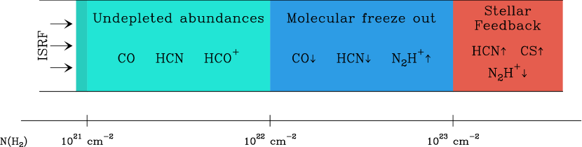
Figure 7: Cartoon view of the main chemical regimes identified in the observed clouds. The labels refer to representative species observed in each regime, and the arrows indicate their abundance trends. The numerical values on the horizontal scale represent approximate estimates of the column density at which the transition between the regimes occurs. This plot is inspired by Fig. 12 of Bergin & Tafalla (2007).

To summarize, our comparison shows that the stratified random sampling method can be used to estimate line luminosities that agree with previously published values at the a level typically better than about 30%. This result is reassuring in view of the large differences in the observing techniques, spatial coverage, calibration schemes, and size of the telescopes involved in the comparison. Our comparison also shows that to obtain accurate luminosity estimates, both techniques require special care. The sampling technique requires using high-quality extinction maps to estimate the surface area subtended by each column density bin, and sampling the emission down to column densities of around 1-$2\times 10^{21}$ cm^-2. The mapping technique requires good spatial coverage of the cloud and the ability to account for the weak emission from the outer parts of the cloud, whose contribution to the luminosity is not negligible due to their large surface area and cannot be masked out.

Having validated the method, we calculated luminosities for all the lines studied in the previous sections, and the results are summarized in Table 6. It should be noted that the N₂H⁺(1–0) values represent only lower limits because the emission of this line was not detected in the outer layers of the cloud, and their potential contribution cannot be estimated with our data. Further discussion of the HCN(1–0) luminosities and their relation with the amount of dense gas in the clouds is deferred to Sect. 4.2.

Table 6: Line luminosity estimates.

Line	Luminosity	Line	Luminosity
	(K km s-1 pc2)		(K km s-1 pc2)
California
12CO(1–0)	35,200	CS(2–1)	78
13CO(1–0)	4,220	HNC(1–0)	68
C18O(1–0)	226	HCO+(1–0)	173
HCN(1-0)	210	N2H+(1–0)	$\geq 8$
Perseus
12CO(1–0)	6,900	12CO(2–1)	5,850
13CO(1–0)	1,160	13CO(2–1)	938
C18O(1–0)	83	C18O(2–1)	61
HCN(1–0)	77	HNC(1–0)	30
CS(2–1)	61	HCO+(1–0)	82
N2H+(1–0)	$\geq 9$
Orion A
12CO(1–0)	28,200	12CO(2–1)	20,100
13CO(1–0)	4,070	13CO(2–1)	4,150
C18O(1–0)	234	C18O(2–1)	316
HCN(1–0)	524	HNC(1–0)	210
CS(2–1)	236	HCO+(1–0)	544
N2H+(1–0)	$\geq 36$

4 Discussion

4.1 The three main chemical regimes of a molecular cloud

The similar dependence on $N$(H₂) and $T_{\mathrm{gas}}$ of the line intensities in California, Perseus, and Orion A suggests that the three clouds share a similar chemical structure, and that this structure can be described using $N$(H₂) and $T_{\mathrm{gas}}$ as the main physical parameters. In this section we combine the results of our analysis of the intensity distributions in the three clouds with the results of the radiative transfer model of the Perseus cloud presented in Paper I to determine the main characteristics of the chemical structure of the clouds. A cartoon view of the proposed structure is presented in Fig. 7.

We start our discussion with the cloud outermost layers. Their chemical composition can only be studied using the few species that are bright enough to be detected toward the lowest column density bins. As shown in Figs. 1 and 2, the emission of both ¹²CO and ¹³CO is detected at all column densities, and presents a sharp change around $N$(H₂) = 1-$2\times 10^{21}$ cm^-2, which is equivalent to a visual extinction of $A_{\mathrm{V}}=1$-2 mag . Similar sharp changes of the CO emission have been seen toward the edges of other molecular clouds (Pineda et al., 2008; Ripple et al., 2013), and they most likely result from the photodissociation of CO by the interstellar radiation field (van Dishoeck & Black, 1988; Wolfire et al., 2010).

As discussed in Paper I, the Perseus data also show hints that the intensity of some traditional dense-gas tracers present an outer change similar to CO, and that some UV-sensitive species, such as C₂H and CN present slight outer abundance enhancements in agreement with the expectations from models of photodissociation regions (Cuadrado et al., 2015). All these effects indicate that in the three clouds, the column density value of 1-$2\times 10^{21}$ cm^-2 marks the approximate boundary between the outer UV-dominated regime and the shielded cloud interior, where most molecular species seem to keep approximately constant abundances (as suggested by the radiative transfer model of Paper I). In Fig. 7, we represent this region as the outermost layer of the cloud, and label its interior as the regime of ”undepleted abundances.”

The next significant change in the cloud chemical composition seems to occur after the column density has increased by about one order of magnitude. The plots of N₂H⁺ intensity show that this tracer experiments an order of magnitude increase between $10^{22}$ and $2\times 10^{22}$ cm^-2, after which the intensity approximately follows quasi-linearly $N$(H₂) (Fig. 5). As mentioned in Sect. 3.6, this sharp increase in the N₂H⁺ abundance is expected to correspond to the onset of CO freeze-out onto the dust grains, and is a consequence of the gradual increase in the gas volume density as the column density increases. The occurrence of this onset at similar column densities in California, Perseus, and Orion A points to a similar increase in the gas volume density as a function of column density in the three clouds, which suggests that the clouds share an important similarity in their internal structure. Since the freeze-out of CO is accompanied by a similar freeze-out of other carbon species such as CS, HCO⁺, and HCN (Kuiper et al., 1996; Tafalla et al., 2006), we interpreted the column density value of $10^{22}$ cm^-2 as an approximate boundary of the second regime of the cloud, which we call the molecular freeze-out regime (Fig. 7).

The final chemical regime suggested by our observations has a less sharp boundary, but approximately corresponds to column densities in excess of $10^{23}$ cm^-2. This regime is only present in the Orion A cloud since California and Perseus do not reach such high values of $N$(H₂), and is represented by the high-mass star-forming regions in the ISF. As discussed in Sect. 3.5, these regions present elevated gas temperatures (¿30 K) and abundance enhancements in selected species such as HCN and CS, and are likely the result of high-temperature chemistry triggered by high-mass star formation. This regime therefore represents the effect of stellar feedback on the cloud gas, and its properties likely depend less systematically on $N$(H₂) than the other two regimes due to the more stochastic nature of the star-formation activity. Given that our sampling of column densities larger than $10^{23}$ cm^-2 is limited to only Orion A, observations of other high-mass star-forming regions are still required to properly characterize this chemical regime.

4.2 HCN as a dense-gas tracer

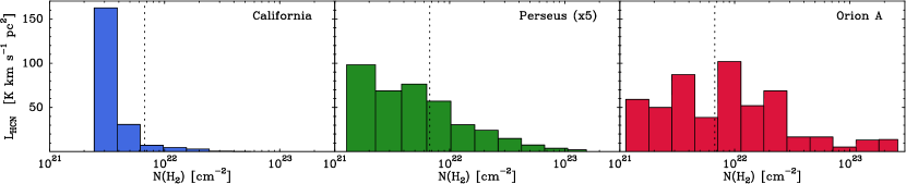
Figure 8: Contribution to the HCN(1–0) luminosity of the different H₂ column density bins to which each cloud has been assigned. The vertical dashed line indicates the column density corresponding to $A_{\mathrm{K}}=0.8$ mag, proposed by Lada et al. (2010) as the boundary of the cloud dense gas. For the California cloud, no HCN(1–0) emission was detected toward the lowest column density bin, so its contribution to the luminosity has been set to zero (see the main text).

Due to its bright lines, HCN has become the tracer of choice to estimate the amount of dense gas in extragalactic studies of star formation. In their classical analysis of the HCN emission from a wide variety of galaxies, Gao & Solomon (2004) found a close-to-linear correlation between the far-IR luminosity and the HCN(1–0) luminosity, and interpreted it as indicating that the star-formation rate of a galaxy depends on the amount of dense gas traced by HCN. To determine the mass of the dense gas associated with the HCN emission, Gao & Solomon (2004) used a combination of large velocity gradient (LVG) radiative transfer and virial analysis, and concluded that

$$M_{\mathrm{dense}}=\alpha(\mathrm{HCN})\;L_{\mathrm{HCN}},$$ (3)

with a conversion factor $\alpha$(HCN) of around 10 M_⊙ (K km s^-1 pc²)^-1. Although Gao & Solomon (2004) recognized the approximate nature of their $\alpha$(HCN) estimate, and stated that an accurate determination required “further extensive studies,” their proposed value has become a de facto standard for extragalactic studies of star formation (e.g., Usero et al. 2015; Gallagher et al. 2018; Jiménez-Donaire et al. 2019).

As mentioned in Sect. 3.4, recent studies of the emission from galactic clouds have shown than HCN(1–0) is not a truly selective tracer of the dense gas since its cloud-scale emission is dominated by the contribution from extended and relatively low density gas (Kauffmann et al., 2017; Pety et al., 2017; Watanabe et al., 2017; Shimajiri et al., 2017; Evans et al., 2020; Tafalla et al., 2021; Dame & Lada, 2023). While this result calls into question a literal interpretation of the $\alpha$(HCN) derivation by Gao & Solomon (2004), the existence of a tight linear correlation between the HCN luminosity and the far-IR luminosity, a reliable tracer of the star formation rate, still indicates that HCN traces either the amount of dense gas or a gas property that is closely connected to the star-forming material. Understanding the origin of the Gao & Solomon (2004) relation therefore remains an open question whose answer requires investigating the origin of the HCN(1–0) emission from local clouds.

To investigate the role of the HCN emission as a dense-gas tracer, we used our sampling data to evaluate the HCN conversion factor in the California, Perseus, and Orion A clouds. Before discussing the results, it should be noted that there are multiple definitions of the HCN conversion factor in the literature (e.g., see Table A.2. in Shimajiri et al. 2017), so it is important to first clarify how the conversion factor is defined. Broadly speaking, two types of definitions have been proposed depending on whether the factor is considered as a global cloud parameter or a a local quantity that varies with the line of sight. Each type of definition focuses on a different aspect of the relation between the HCN emission and the cloud gas, and provides a useful clue to the origin of the HCN emission. We therefore discuss them in sequence.

4.2.1 The global $\alpha_{08}$(HCN) factor

The global $\alpha$(HCN) factor relates the cloud-integrated HCN(1–0) luminosity to the total mass of the dense gas, and follows the spirit of the original Gao & Solomon (2004) definition as given in Eq. 3. This factor is most relevant for extragalactic observations since they do not resolve the emission from individual clouds and therefore need to rely on cloud-integrated quantities. In their original derivation, Gao & Solomon (2004) assumed that the HCN emission was truly selective of the dense gas, and estimated that $\alpha$(HCN) was approximately equal to $2.1\,\langle n(\mathrm{H}_{2})\rangle^{1/2}/T_{\mathrm{b}}$ $M_{\sun}$(K km s^-1 pc²)^-1, where $\langle n(\mathrm{H}_{2})\rangle$ is the average gas density and $T_{\mathrm{b}}$ is the line brightness temperature. Assuming that these parameters take values of $3\times 10^{4}$ cm^-3 and 35 K, respectively, Gao & Solomon (2004) derived the often-used result that $\alpha\mathrm{(HCN)}\approx 10$ $M_{\sun}$(K km s^-1 pc²)^-1. Since we now know that the HCN emission is not truly selective of the dense gas (Kauffmann et al., 2017; Pety et al., 2017; Watanabe et al., 2017; Shimajiri et al., 2017; Evans et al., 2020; Tafalla et al., 2021; Dame & Lada, 2023), it has become customary to determine the value of the global $\alpha$(HCN) factor by defining the amount of dense gas using an independent criterion, such as the amount of mass over an extinction threshold of $A_{\mathrm{K}}=0.8$ mag, which seems to correlate with the star-formation rate of a cloud (Lada et al. 2010; see also Evans et al. 2014). From now on, we refer to this definition of the conversion factor as $\alpha_{0.8}$(HCN).

In Sect. 3.7 we show how the sampling data can be used to derive line luminosities, and present estimates for HCN and other species in each of out sample clouds (Table 6). To better understand how the HCN(1–0) luminosity arises from the different layers of each cloud, we now present in Fig. 8 histograms of the luminosity as a function of $N$(H₂) for California, Perseus, and Orion A. Each bin in the histogram corresponds to a column density bin of our sampling, and the dotted vertical lines mark the $A_{\mathrm{K}}=0.8$ mag threshold used to define the dense gas ($\approx 6.7\times 10^{21}$ cm^-2; e.g., Lombardi et al. 2014). In the California cloud, no HCN(1–0) emission was detected in the average spectrum of the lowest column density bin, so we set its line contribution to zero, while in Perseus and Orion A the HCN(1–0) emission was detected even in the lowest column density bin.

As can be seen in the figure, the highest column density bins contribute the least to the HCN luminosity in each cloud. This occurs because despite their brighter lines, these high column density bins cover a very small area, so their contribution to the total luminosity cannot compete with that of the weaker but much more extended emission from the low column density gas. Using the $A_{\mathrm{K}}=0.8$ mag threshold as a boundary for the dense gas, our data indicate that the high density material only contributes to the total HCN(1–0) luminosity by 8% in California, 37% in Perseus, and 55% in Orion A (Table $a$). Our estimate for Perseus is very close to the 40% estimated by Dame & Lada 2023 from their mapping observations, and a similar range of values has been determined for clouds in the inner and outer Galaxy by Evans et al. (2020) and Patra et al. (2022), respectively.

Table 7: Dense gas masses, HCN(1–0) luminosities, and global HCN conversion factors.

Cloud	$M_{08}$	$L_{\mathrm{T}}$[HCN(1–0)]	$L_{08}$[HCN(1–0)]	$f_{08}$	$\alpha_{08}$(HCN)
	[$M_{\sun}$]	[K km s-1 pc2]	[K km s-1 pc2]		[$M_{\sun}$(K km s-1 pc2)-1]
California	4,800	210	16	0.08	23
Perseus	5,600	77	28	0.37	73
Orion A	24,000	524	290	0.55	46

The low (and variable) contribution from the high density gas to the total HCN luminosity of California, Perseus, Orion A, and other clouds shows that if the HCN luminosity is proportional to the amount of star-forming gas in a cloud, it is not because HCN traces that gas directly, but may be because it acts as a proxy of the star-forming material (Jiménez-Donaire et al., 2023). With this caveat in mind, we determined the amount of dense gas ($M_{08}$) in each cloud by integrating the H₂ column density over the 0.8 mag threshold in the maps of Lombardi et al. (2014), Zari et al. (2016), and Lada et al. (2017), and assuming a solar value for the metallicity (Asplund et al., 2021). Dividing the derived dense-gas masses by the HCN(1–0) luminosities, we estimated the $\alpha_{08}$(HCN) factors reported in Table $a$. As can be seen, our $\alpha_{08}$(HCN) estimates span more than a factor of 3, and range (in units of $M_{\sun}$(K km s^-1 pc²)^-1) from 23 for California to 73 in Perseus, with Orion A having an intermediate value of 46. We note that our estimate for Perseus is very close to the 76 $M_{\sun}$(K km s^-1 pc²)^-1 derived by Dame & Lada (2023) when these authors take into account the contribution of the HCN emission that lies outside their mapping boundary. Our value for Orion A, on the other hand, is more than a factor of 2 higher than the value estimated by Kauffmann et al. (2017), most likely due to a different estimate of the HCN luminosity, while no determination of $\alpha_{08}$(HCN) for California had so-far been presented. Taken together, our estimates suggest that $\alpha_{08}$(HCN) varies between clouds, and that no single HCN conversion factor can be used as a reference value. A similar diversity of conversion factors has been found by Evans et al. (2020) and Patra et al. (2022). In our case, all values are significantly larger than the canonical 10 $M_{\sun}$(K km s^-1 pc²)^-1 derived by Gao & Solomon (2004) and commonly used in extragalactic work (Usero et al., 2015; Gallagher et al., 2018; Jiménez-Donaire et al., 2019).

While our sample of three clouds is too small to investigate in general the origin of the $\alpha_{08}$(HCN) variations, it already offers some clues on what cloud properties are likely to affect the value of $\alpha_{08}$(HCN). A first property to consider is the gas temperature, which we have seen in previous sections significantly influences the intensity of most molecular lines. A dependence of $\alpha_{08}$(HCN) on temperature was already predicted by Gao & Solomon (2004), who derived a $1/T_{\mathrm{b}}$ scaling from their original estimate. While these authors used the line brightness temperature as a parameter instead of the more physical gas kinetic temperature, it is expected that the two will be related even if the lines are not fully thermalized. In this regard, it is interesting to note that Gao & Solomon (2004) assumed an HCN(1–0) brightness temperature of 35 K, which may have been correct for some of the ultra-luminous IR galaxies of their sample, but is clearly too large for the galactic clouds of our study. This can seen from Fig. B.2 in Tafalla et al. 2021, which shows that the HCN(1–0) line toward the densest parts of Perseus reaches a brightness temperature that is a full order of magnitude lower than assumed by Gao & Solomon (2004). As a result, even a simple application of the $T_{\mathrm{b}}$ scaling law predicts a conversion factor close to 100 $M_{\sun}$(K km s^-1 pc²)^-1, which is closer to the value we derive for Perseus. Since we now know that the Gao & Solomon (2004) estimate is too simple an approximation, it is critical to determine how $\alpha$(HCN) depends on temperature with real data. While this cannot be done using our limited sample of clouds, it can be investigated using the local version of $\alpha$(HCN), and for this reason, we defer further discussion of the temperature effects to the next subsection.

Another parameter that affects the value of $\alpha_{08}$(HCN) and can cause variations between clouds is the contribution from the outermost cloud layers. As illustrated in Fig. 8, these layers contribute significantly to the total HCN luminosity, but since they do not contribute to the amount of dense gas, their net effect is to decrease the value of $\alpha_{08}$(HCN). The most extreme example of this effect is seen in the California cloud, where about 92% of the HCN luminosity emerges from regions below the $A_{\mathrm{K}}=0.8$ mag dense-gas threshold (the fraction is 63% in Perseus and 45% in Orion A; see Table $a$). Not surprisingly, California presents the lowest $\alpha_{08}$(HCN) value of our sample (23 $M_{\sun}$(K km s^-1 pc²)^-1), which is about half that of Orion A and one third of that of Perseus. While California may represent an extreme example of a cloud in terms of its diffuse structure Lada et al. (2017), Perseus and Orion A also present significant differences in terms of the contribution from their outer layers to the HCN luminosity, an effect also seen by Evans et al. (2020) toward clouds in the inner galaxy. While it may be possible that any cloud-to-cloud differences average out in extragalactic observations that contain multiple clouds inside a telescope bin, it is likely that a multiplicity of $\alpha_{08}$(HCN) values is intrinsic to any cloud population.

We finish our analysis of the global $\alpha_{08}$(HCN) factor by noting that the potentially large contribution from the outer layers to the HCN(1–0) luminosity imposes a serious difficulty in estimating HCN(1–0) luminosities and therefore $\alpha_{08}$(HCN) factors both to the mapping and sampling techniques. Our observations of Perseus and Orion A show that there is residual HCN(1–0) emission even in the lowest column density bins of these clouds, whose extinction is in the range to $A_{\mathrm{V}}\approx$ 1-2 mag. Any observation that does not sample this low-extinction regime runs therefore the risk of underestimating the total luminosity and therefore overestimating the $\alpha_{08}$(HCN) factor. For the California cloud, the HCN(1–0) line was not detected in the lowest column density bin, and from the rms level of the average spectrum we estimate that the possible contribution from this bin is on the order of 10% of the total luminosity, although the figure is clearly uncertain. A shown in Sect. 3.7, our luminosity estimate of the more extended CO(1–0) emission matches the independent estimate of Lewis et al. (2022), so we have some confidence that the sampling technique can provide a meaningful estimate of the HCN luminosity even if dominated by the cloud outermost layers.

4.2.2 The local $\alpha_{\mathrm{X}}$(HCN) factor

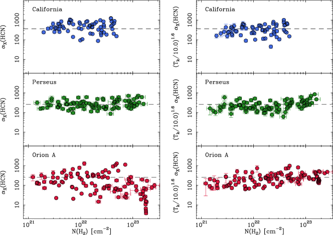
Figure 9: Local $\alpha_{\mathrm{X}}$(HCN) factor as a function of H₂ column density for the California, Perseus, and Orion A clouds. Left: $\alpha_{\mathrm{X}}$(HCN) factor calculated using Eq. 4. Right: $\alpha_{\mathrm{X}}$(HCN) factor multiplied by the temperature factor ($T_{\mathrm{k}}$/10 K)^1.6 to compensate for the dependence determined in Eq. 5. Note the reduced dispersion of the Orion A data. In all panels, the units of $\alpha_{\mathrm{X}}$(HCN) are in M_⊙ (K km s^-1 pc²)^-1, and the dashed lines represent the mean value of the temperature-corrected factor for each cloud.

We now investigate the information about the HCN(1–0) emission as a dense-gas tracer that can be derived from the local definition of the conversion factor. This definition follows common practice in the analysis of the CO emission as a cloud tracer, where the term conversion factor is referred indistinctly to both the ratio between H₂ column density and integrated intensity (represented by $X$), and the ratio between total cloud mass and line luminosity (represented by $\alpha$; see Bolatto et al. 2013 for a review). Following this convention, we define

$$\alpha_{\mathrm{X}}(\mathrm{HCN})\;[\mathrm{M}_{\odot}\leavevmode\nobreak\ (\mathrm{K\leavevmode\nobreak\ km\leavevmode\nobreak\ s}^{-1}\mathrm{\leavevmode\nobreak\ pc}^{2})^{-1}]=2.25\times 10^{-20}\;\frac{N{\mathrm{(H}}_{2}\mathrm{)\;[cm}^{-2}]}{I_{\mathrm{HCN}}\;\mathrm{[K\leavevmode\nobreak\ km\leavevmode\nobreak\ s}^{-1}]},$$ (4)

where we have assumed a solar abundance of the elements (Asplund et al., 2021) to convert the H₂ column density into a mass density, and used the subindex X following the convention proposed by Dame & Lada (2023) (see, e.g., Eq. 7 in Evans et al. (2022) for an equivalent definition using CO). As expected from Eq. 4, the global and local conversion factors are closely related: the global factor corresponds to the intensity-weighted cloud average of the local factor after substituting the total H₂ column density by the column density of dense gas.

The local $\alpha_{\mathrm{X}}$(HCN) factor has been used by Shimajiri et al. (2017) to investigate the relation between the HCN emission and the gas mass in the Aquila, Ophiuchus, and Orion B clouds (see their Fig. 6). Our sampling observations provide a natural data set to carry out a similar investigation in California, Perseus, and Orion A since the ratio between the H₂ column density and the HCN(1–0) intensity can be directly determined from the sampling data. The left panels of Fig. 9 show the distribution of $\alpha_{\mathrm{X}}$(HCN) as a function of $N$(H₂) for California, Perseus, and Orion A when no temperature correction has been applied to the HCN emission. As can be seen, the $\alpha_{\mathrm{X}}$(HCN) parameter remains approximately constant in California and Perseus, as expected from the close-to-linear dependence of the HCN(1–0) intensity on $N$(H₂) found in Sect. 3.4. In addition, it presents relatively low levels of dispersion of 0.27 and 0.21 dex, respectively. The $\alpha_{\mathrm{X}}$(HCN) parameter in Orion A, on the other hand, remains approximately constant for $N$(H₂) lower than $10^{23}$cm^-2 but drops significantly at higher column densities and presents a higher level of scatter of about 0.53 dex. Overall, our $\alpha_{\mathrm{X}}$(HCN) distributions look similar to those found by Shimajiri et al. (2017) in Aquila, Ophiuchus, and Orion B, which show close-to-constant dependence on extinction. The Perseus distribution, in addition, presents a similar average to that determined by Dame & Lada (2023) for this cloud (=215), as would have been expected from their similar estimate of the $X$ factor.

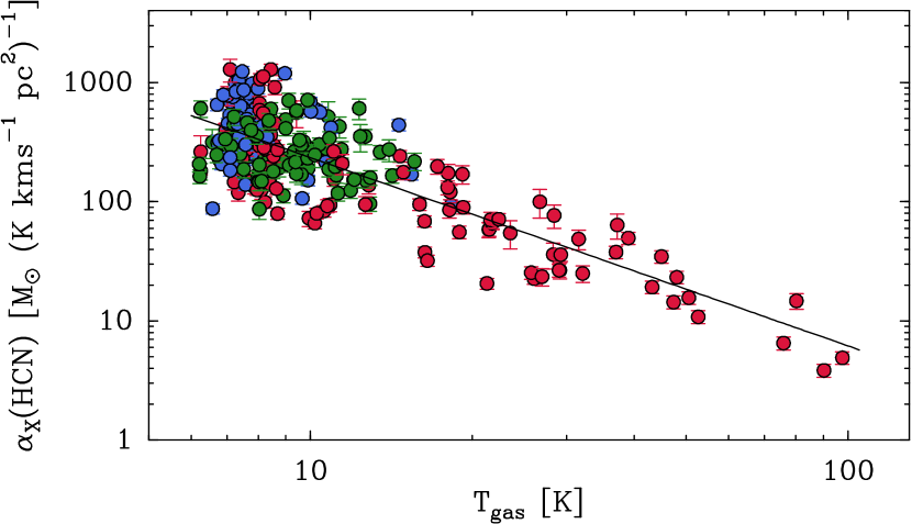
Figure 10: $\alpha_{\mathrm{X}}$(HCN) factor as a function of gas temperature in California, Perseus, and Orion A. The solid line represents the fit described in the text. The data are color-coded as in previous figures.

To investigate the origin of the higher dispersion of $\alpha_{\mathrm{X}}$(HCN) in Orion A, we looked at the dependence of the HCN emission on temperature. Section 3.4 and previous studies of the HCN(1–0) emission in Orion A have found a systematic dependence of the emission on temperature (Goldsmith et al. 1981; Schilke et al. 1992; Graninger et al. 2014), and Hacar et al. (2020) estimated that the ratio between HCN(1–0) intensity and visual extinction depends quadratically on the gas kinetic temperature up to 40 K (these authors excluded from their analysis the hottest vicinity of the ONC). Figure 10 presents our estimate of the dependence of the $\alpha_{\mathrm{X}}$(HCN) factor on gas temperature for the combined data from California, Perseus, and Orion A. As can be seen, at low temperatures ($\sim 10$ K) the data from the three clouds shows a significant overlap, while at higher temperatures (¿ 15 K), which are only represented by the Orion A data, $\alpha_{\mathrm{X}}$(HCN) systematically decreases with temperature by almost two orders of magnitude. From a linear fit to the log-log plot we determine that $\alpha_{\mathrm{X}}$(HCN) depends on the gas kinetic temperature as

$$\alpha_{\mathrm{X}}(\mathrm{HCN})\;[\mathrm{M}_{\odot}\leavevmode\nobreak\ (\mathrm{K\leavevmode\nobreak\ km\leavevmode\nobreak\ s}^{-1}\mathrm{\leavevmode\nobreak\ pc}^{2})^{-1}]=235\pm 41\;\left(\frac{T_{\mathrm{gas}}}{10\leavevmode\nobreak\ \mathrm{K}}\right)^{-1.6\pm 0.1}.$$ (5)

This dependence of $\alpha_{\mathrm{X}}$ on the gas kinetic temperature is steeper than the $T_{\mathrm{b}}^{-1}$ predicted by Gao & Solomon (2004) (assuming a close relation between the brightness and kinetic temperatures). This is likely the result from a combination of our more realistic dependence of the line intensity on the gas temperature (Appendix D.2) and the high sensitivity of the HCN abundance with gas temperature found in Sect. 3.5.

The systematic correlation of $\alpha_{\mathrm{X}}$(HCN) with gas temperature suggests that the peculiar behavior of the Orion A data in Fig. 9 results from the temperature variations in the cloud. To test this idea, we multiplied the $\alpha_{\mathrm{X}}$(HCN) factor by ($T_{\mathrm{k}}$/10 K)^1.6, which is the inverse of the power law derived from the fit, and present the result in the right panels of Fig. 9. As can be seen, the temperature-corrected conversion factor in Orion A shows an approximately constant dependence on $N$(H₂) and has a similar dispersion to that measured in California and Perseus (0.2-0.3 dex). A slight drop of $\alpha_{\mathrm{X}}$(HCN) al low $N$(H₂) in the temperature-corrected values of Perseus and Orion A likely results from small errors in the temperature at low column densities when using the dust temperature as a reference (Sect. 3.2).

The similar distribution of the corrected $\alpha_{\mathrm{X}}$(HCN) factors in the three clouds suggests that gas temperature differences were responsible for the observed differences in the uncorrected factors. This interpretation differs from that of Shimajiri et al. (2017), who also found differences in the conversion factor between their clouds, but associated them with variations in the local far-UV (FUV) radiation field, which they estimated to range from $G_{0}=1$ to more than 4000. Interpreting the $\alpha_{\mathrm{X}}$(HCN) differences as a result of the FUV radiation, however, presents several problems. First of all, it is unlikely that the HCN-emitting gas is directly exposed to the high levels of FUV radiation measured toward the exterior of the clouds since UV radiation quickly photodissociates the HCN molecules (Aguado et al., 2017). In addition, a dependence of $\alpha_{\mathrm{X}}$(HCN) on the external FUV radiation field seems to contradict the observed constant behavior of this factor as a function of column density since the FUV radiation is expected to be strongly attenuated by the cloud internal extinction. It is therefore more likely that the cloud-to-cloud variations found by Shimajiri et al. (2017) also arise from differences in the cloud gas temperature. This is further supported by the fact that Shimajiri et al. (2017) used the dust temperature to infer the $G_{0}$ factor, so there is a possible ambiguity interpreting the effect of the two parameters.

If the gas temperature has the strong effect on the local $\alpha_{\mathrm{X}}$(HCN) factor suggested by Eq. 5, a similar dependence on temperature is expected to affect the global factor, which we have seen represents an intensity-weighted average of $\alpha_{\mathrm{X}}$(HCN) over a whole cloud. This temperature dependence may be difficult to observe in nearby galactic clouds because the contribution from relatively warm regions will likely be overwhelmed by the contribution from the more extended colder gas that we have seen dominates the HCN emission. In extragalactic observations, on the other hand, it may be possible to encounter more extreme conditions where the warm gas dominates the global HCN emission. Indeed, observations of luminous and ultra-luminous infrared galaxies suggest that these systems have significantly lower conversion factors than normal galaxies (García-Burillo et al., 2012), as expected from their elevated gas temperatures. This result should serve as a warning that for neither the local nor the global versions of the conversion factor, one size fits all, and that care must be exercised when applying the same conversion factor to inhomogeneous samples of clouds or galaxies.

4.3 The HCN/CO ratio and its correlation with the H₂ column density

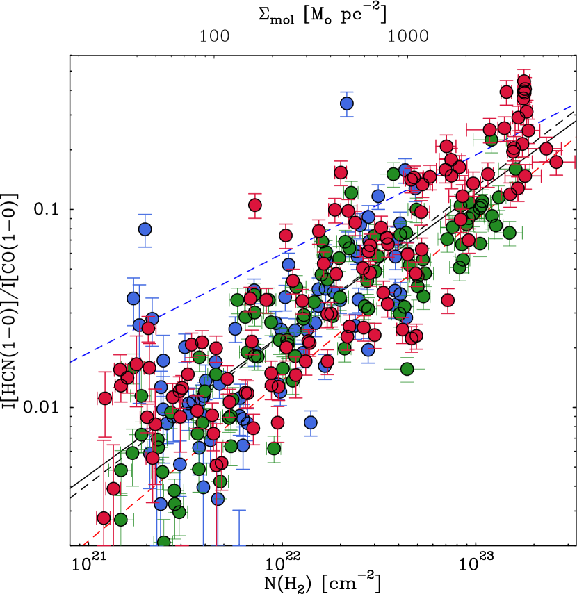
Figure 11: HCN(1–0)/CO(1–0) intensity ratio as a function of H₂ column density for California, Perseus, and Orion A, color-coded as in Fig. 1. The solid and dashed black lines represent the two fits discussed in the text. The dashed red and blue lines represent, respectively, the fits derived by Gallagher et al. (2018) and Jiménez-Donaire et al. (2019) from extragalactic data.

Another parameter commonly used to interpret extragalactic observations is the HCN/CO intensity ratio. Assuming that the HCN intensity is proportional to the dense gas column density, and that the CO intensity is proportional to the total gas column density, the HCN/CO intensity ratio is expected to measure the fraction of dense gas (Gao & Solomon, 2004; Usero et al., 2015; Leroy et al., 2017). Recent work by Gallagher et al. (2018) and Jiménez-Donaire et al. (2019) has found a significant correlation between the HCN/CO ratio and the molecular column density in (normal) galaxies averaged over 1-2 kpc spatial scales. Gallagher et al. (2018) have interpreted this correlation as indicating that both the HCN/CO ratio and the gas column density are sensitive tracers of the density distribution in molecular clouds.

Our line survey provides estimates of the HCN and CO intensity together with the $N$(H₂) column density, so we can use the data to investigate the correlation between the HCN/CO ratio and $N$(H₂) in galactic clouds. Figure 11 presents the HCN(1–0)/CO(1–0) intensity ratio (HCN/CO hereafter) for the three clouds of our survey as a function of both the H₂ column density (lower x-axis) and the molecular surface density commonly used in extragalactic work (upper x-axis). No temperature correction has been applied to either the HCN or CO data, so the results can be directly compared with extragalactic observations. Applying a temperature correction to the two lines, however, only has a minor effect on the intensity ratio since the two corrections almost cancel out and the resulting scatter plot is practically indistinguishable from that of Fig. 11. As can be seen in the figure, the HCN/CO ratio correlates strongly with the H₂ column density over the more than two orders of magnitude covered by this parameter. In addition, the correlation seems to be the same in the three clouds, an impression confirmed by FF tests of the three possible cloud pairs, which return p-values between 0.28 and 0.76. Combining the data from the three clouds, we estimate a Pearson’s coefficient of 0.84 (in log-log scale), and using a least squares fit we derive a relation of the form

$$\log_{10}\left(\frac{I_{\mathrm{HCN}}}{I_{\mathrm{CO}}}\right)=(-3.3\pm 0.8)+(0.71\pm 0.03)\;\log_{10}\left(\frac{\Sigma_{\mathrm{mol}}}{{\mathrm{M}_{\sun}\;\mathrm{pc}^{-2}}}\right),$$ (6)

where the intensities refer to the $J$=1–0 transition of both HCN and CO. This fit is represented in the figure by a black solid line.

The correlation between HCN/CO and $N$(H₂) found in our three clouds is remarkably similar to that seen at kiloparsec scales in external galaxies by Gallagher et al. (2018) and Jiménez-Donaire et al. (2019). These extragalactic observations cover similar ranges of $N$(H₂) as our cloud data ($10^{2}$-$10^{3}$ M_⊙ pc^-2 for Gallagher et al. 2018 and 10-300 M_⊙ pc^-2 for Jiménez-Donaire et al. 2019, although these values include the contribution of the filling factor of the clouds), and are illustrated in Fig. 11 using red and blue dotted lines. As the plot shows, our galactic fit, with a slope of $0.71\pm 0.03$, is intermediate between the fits obtained by Gallagher et al. (2018) (slope $0.81\pm 0.09$) and Jiménez-Donaire et al. (2019) (slope $0.5\pm 0.1$), who used different assumptions to estimate the molecular surface density.

Further work is needed to better connect the galactic and extragalactic results, both in terms of the disparate spatial scales that they sample (subparsec and 1-2 kpc, respectively) and the different methods used to derive the H₂ column density, which in the extragalactic case relies on indirect uses of the CO emission (Gallagher et al., 2018; Jiménez-Donaire et al., 2019). Assuming that the different estimates are truly comparable, the most natural interpretation of the similar behavior of the HCN/CO ratio is that the extragalactic correlation reflects the internal properties of the individual unresolved clouds. To explore how these properties could give rise to the HCN/CO versus $N$(H₂) correlation seen in our data set, we needed to use the results from the radiative transfer model presented in Paper I to reproduce the Perseus data. The similar behavior of the HCN/CO ratio in the three clouds of our sample suggests that the excitation mechanism responsible for the Perseus correlation is likely also responsible for the California and Orion A correlations.

According to Paper I, the intensity of multiple transitions, including CO(1–0) and HCN(1–0), can be reproduced with a model that assumes that the gas physical and chemical properties depend on $N$(H₂) (see Table 3 in Paper I). Of particular interest for the HCN/CO correlation is the relation between the volume density and the column density, which was found to have the form $n(\mathrm{H}_{2})=2\times 10^{4}\mathrm{cm}^{-3}\;(N$(H${}_{2})/10^{22}\mathrm{cm}^{-2})^{0.75}$. Using this relation, the radiative transfer model of Paper I showed that both CO(1–0) and HCN(1–0) must be optically thick over most of the cloud, and that while CO(1–0) is thermalized at all column densities, HCN(1–0) remains sub-thermal with an excitation temperature strongly dependent on $N$(H₂) (see Fig. 13 in Paper I). This excitation behavior makes the intensity of HCN(1–0) rapidly increase with $N$(H₂) (through its density dependence), while the intensity of CO(1–0) stays approximately constant. As a result, the HCN/CO ratio systematically increases with $N$(H₂), in agreement with the observed behavior.

To next interpret the HCN/CO ratio as an indicator of the gas volume density, we combined the relation between volume and column densities derived in Paper I with our fit of the HCN/CO data. As seen in Eq. 6, the HCN/CO ratio depends on $N$(H₂) with a slope of $0.71\pm 0.03$, which differs by only 1.3 $\sigma$ from the 0.75 value determined for the density relation with $N$(H₂). Taking this similarity of values as an indication of an approximate equality, we re-fitted the HCN/CO-$N$(H₂) correlation using a fixed value of 0.75. The result is represented in Fig. 11 with a dashed line, and is practically indistinguishable from the original best fit inside the range of values covered by the observations. Using this new fit (which has an intercept of -3.4), we derive a relation between gas density and the HCN/CO ratio of the form

$$n(\mathrm{H}_{2})=8.7\times 10^{5}\;\mathrm{cm}^{-3}\;\frac{I_{\mathrm{HCN}}}{I_{\mathrm{CO}}}.$$ (7)

This volume density should be interpreted as a mean value along the line of sight where the HCN/CO ratio has been measured, and since its derivation uses the radiative transfer model of Paper I, the mean has been weighted by the emission of the CS and HCN. No meaningful error bar could be estimated for this density due to the difficulty in quantifying the model assumptions, but given the quality of the model fits, it is likely that the uncertainty lies within a factor of 2.

It is probably premature to extrapolate our derived relation between volume density and HCN/CO ratio to extragalactic data, although the strong similarity between the galactic and extragalactic correlations of HCN/CO with $N$(H₂) suggests that this is likely to be the case. If so, the HCN/CO ratio should be thought not so much as an indicator of the dense gas fraction but as an estimator of the gas volume density averaged over the line of sight and the observing beam. Such an estimator presents the advantage over single-line tracers that is less sensitive to gas temperature variations given the approximate cancellation between the dependences of HCN and CO. Further characterization of the HCN and CO emission from galactic clouds is needed to study the general properties of the line ratio and to better calibrate its dependence on $N$(H₂). For this investigation, the stratified random sampling technique presented here appears to be a suitable tool.

5 Conclusions

We sampled the 3 mm wavelength emission of the California and Orion A clouds using the IRAM 30 m radio telescope. We selected a set of target positions using the stratified random sampling technique previously used in Tafalla et al. (2021) to study the emission from the Perseus cloud. This technique divides the cloud into multiple bins of H₂ column density and randomly selects a number of cloud positions in each bin to carry out the molecular-line observations. We combined the new results from California and Orion A with the Perseus cloud data to investigate the main gas parameters that control the line emission of the CO isotopologs and the main dense-gas tracers, and to compare the emission of these species in three clouds whose star-formation rates span more than one order of magnitude. The main results from our study are the following:

1. In the three target clouds, the intensity of the studied molecular lines correlates strongly with the value of the H₂ column density even if the positions are separated by distances of tens of parsecs. This strong correlation with $N$(H₂) shows that this parameter is the main predictor of the line intensity and supports its use in the stratified random sampling technique.

2. The observations of Orion A, which presents gas temperature variations across its components, show that the intensity of most molecular lines also depends on the gas temperature. We used a cloud radiative transfer model to determine the expected change in the intensity of all target lines as a function of gas temperature, and used the model results to simulate the emission expected if our target clouds were isothermal. The temperature-corrected intensities present a lower level of dispersion and a better agreement between the three target clouds than the uncorrected intensities.

3. We find that the temperature-corrected intensity of the CO lines has a flatter-than-linear dependence on $N$(H₂), while the intensity of traditional dense-gas tracers such as HCN(1–0), CS(2–1), HCO⁺(1–0), and HNC(1–0) scales almost linearly with $N$(H₂) over the two orders of magnitude covered by the observations ($\approx 10^{21}$-$10^{23}$ cm^-2).

4. In contrast with the traditional dense-gas tracers, the intensity of N₂H⁺(1–0) does not correlate linearly with $N$(H₂) over the full column density range. It correlates almost linearly at high column densities, but it drops by more than one order of magnitude between $2\times 10^{22}$ cm^-2 and $10^{22}$ cm^-2, and remains undetected at lower column densities. This behavior, which is similar in the three clouds, makes N₂H⁺ the only selective tracer of the cloud cold dense component.

5. In addition to affecting the molecular excitation, the gas kinetic temperature changes the abundance of some species. Using the intensity distribution of rare isotopologs, we find that the abundance of HCN and CS is systematically enhanced with increasing gas temperature, while the abundance of HCO⁺ and HNC remains approximately constant between 10 and 100 K. In contrast with the classical dense-gas tracers, N₂H⁺ decreases in abundance with temperature, most likely due to the release of CO from the grains as the temperature increases.

6. The stratified random sampling data can also be used to estimate cloud-integrated luminosities of the different molecular lines. We compared our estimated luminosities with literature values (mostly from CO isotopologs) and find an agreement typically at the 25% level, which is remarkable because the comparison involves very different telescopes and calibration schemes. We used our sampling data to estimate luminosities of the main survey lines in California, Perseus, and Orion A.

7. The systematic emission patterns found in our survey suggest that the target molecular clouds share a common chemical structure. This structure is characterized by abundance variations as a function of column density and can be approximately understood as consisting of three main chemical regimes. Between the photodissociation boundary ($\sim 10^{21}$ cm^-2) and $\sim 10^{22}$ cm^-2, most species maintain a close-to-constant abundance that is likely determined by gas-phase reactions. In this regime, N₂H⁺ remains undetected due to the high CO abundance in the gas phase. From $\sim 10^{22}$ cm^-2 to $\sim 10^{23}$ cm^-2, the abundance of most species decreases due to freeze-out onto grains, while N₂H⁺ is enhanced as a result of a decrease in the gas-phase CO abundance. At elevated temperatures and column densities higher than $\sim 10^{23}$ cm^-2, which in our sample are only reached toward Orion A, high-mass star-formation feedback disturbs the gas chemical composition, enhancing species such as HCN and CS and destroying N₂H⁺.

8. We used our survey data to study the relation between the HCN(1–0) emission and the cloud gas mass. We explored the clues provided by two possible definitions of the HCN conversion factor previously used in the literature. The “global” definition compares the cloud-integrated line luminosity with the amount of “dense” gas and shows variations of more than a factor of 3 between California, Perseus, and Orion A. These variations mostly arise from the different contribution to the HCN emission of the external layers of the cloud, which tend to dominate the luminosity due to their large surface area. A “local” definition of the $\alpha$(HCN) factor compares the HCN(1–0) intensity with the total H₂ column density and can be measured at each cloud position. This factor displays a strong dependence on the gas kinetic temperature, which seems to result from a combination of excitation and abundance effects. A dependence of the $\alpha$(HCN) factor on the gas temperature may help explain the diversity of values seen by galactic and extragalactic observers.

9. We also used our survey data to study the correlation between the HCN(1–0)/CO(1–0) intensity ratio and the gas column density, which has recently been studied using extragalactic observations. Our data show a similar relation in terms of both the range of parameters and slope. Using the results of a cloud radiative transfer model, we show that the HCN(1–0)/CO(1–0) ratio can be used to estimate the mean gas volume density, and that the correlation with $N$(H₂) observed in our clouds results from the gradual increase in the HCN(1–0) sub-thermal excitation with H₂ column density.

The above results illustrate the great potential of the stratified sampling technique to characterize the molecular emission from star-forming clouds. Given its relatively low cost in terms of telescope observing time, it should be possible to expand its application to a larger number of clouds and obtain a more complete view of their intrinsic diversity that can further our understanding of star formation and can serve as a template to analyze extragalactic observations.

Appendix A Maps of sample points for California and Orion A

Figures 12 and 13 represent in color scale the column density maps of California and Orion A derived by Lada et al. (2017) and Lombardi et al. (2014). The numbers mark the positions selected using the stratified random sampling technique, and numerical values indicate the column density bin to which the position belongs.

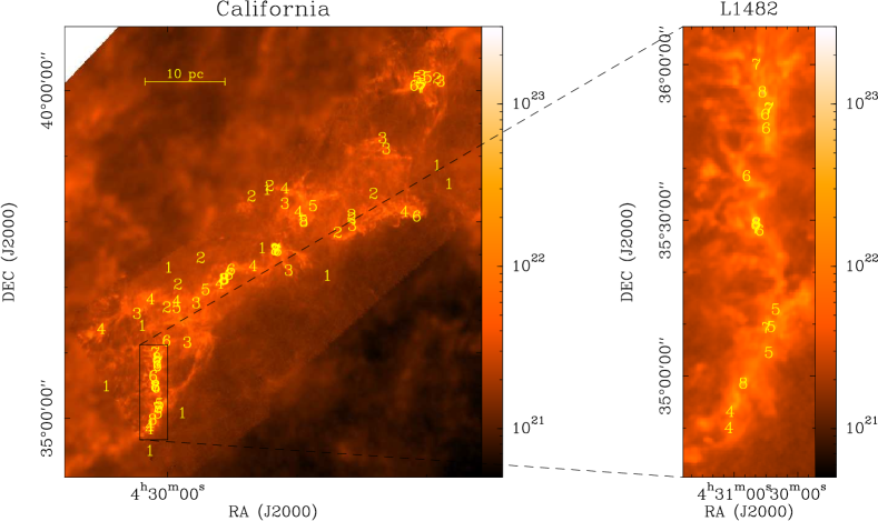
Figure 12: Sampling of the California cloud. The color images represent the distribution of column density as derived by Lada et al. (2017) from Herschel Space Observatory data, and the numbers indicate the positions chosen using stratified random sampling. The right panel is an expanded view of the L1482 region, which contains some of the highest column density positions. The numbers refer to the column density bin of the position (1 is lowest and 8 is highest), the 10 pc scale bar assumes a distance of 470 pc (Zucker et al. 2019), and the wedge scale is in units of cm^-2.

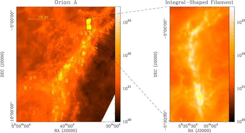
Figure 13: Sampling of the Orion A cloud. The color images represent the distribution of column density as derived by Lombardi et al. (2014) from Herschel Space Observatory data, and the numbers indicate the positions chosen using stratified random sampling. The right panel is an expanded view of the ISF, which contains some of the highest column density positions. The numbers refer to the column density bin of the position (1 is lowest and 12 is highest), the 10 pc scale bar assumes a distance of 432 pc (Zucker et al. 2019), and the wedge scale is in units of cm^-2.

Appendix B Sample positions and 3 mm line intensities

Tables 8 and 9 present the coordinates, H₂ column density estimates, and 3 mm line intensities for all the target positions in the California and Orion clouds. Full versions of the tables are available at the CDS.

Table 8: Sample positions and line intensities for California.

Position	RA(J2000)	Dec(J2000)	$N$(H2)	12CO(1–0)	13CO(1–0)	C18O(1–0)	HCN(1–0)	CS(2–1)
	(h  m  s)	(°  ′  ″)	(cm-2)	(K km s-1)	(K km s-1)	(K km s-1)	(K km s-1)	(K km s-1)
CAL-08_10	04 19 28.8	+37 59 04	$3.81(0.04)\times 10^{22}$	21 (2)	4.6 (0.5)	2.1 (0.2)	0.69 (0.07)	0.65 (0.07)
CAL-08_09	04 25 36.1	+37 06 05	$4.46(0.05)\times 10^{22}$	19 (2)	6.6 (0.7)	2.3 (0.2)	1.1 (0.1)	0.93 (0.09)
CAL-08_08	04 25 40.2	+37 07 01	$3.83(0.03)\times 10^{22}$	18 (2)	5.6 (0.6)	2.4 (0.2)	0.72 (0.07)	0.69 (0.07)
CAL-08_07	04 30 48.5	+34 58 03	$4.31(0.14)\times 10^{22}$	30 (3)	9.9 (1.0)	1.3 (0.1)	4.8 (0.5)	2.8 (0.3)
CAL-08_06	04 30 39.4	+35 29 02	$4.08(0.05)\times 10^{22}$	43 (4)	17 (2)	4.3 (0.4)	1.6 (0.2)	1.4 (0.1)
CAL-08_05	04 25 32.0	+37 07 01	$3.92(0.02)\times 10^{22}$	14 (1)	4.3 (0.4)	1.5 (0.2)	1.0 (0.1)	0.50 (0.05)
CAL-08_04	04 30 36.8	+35 54 03	$4.88(0.12)\times 10^{22}$	56 (6)	17 (2)	3.6 (0.4)	7.2 (0.7)	6.0 (0.6)
CAL-08_03	04 21 41.0	+37 33 05	$4.07(0.07)\times 10^{22}$	31 (3)	8.5 (0.9)	2.5 (0.3)	2.6 (0.3)	2.6 (0.3)
CAL-08_02	04 30 40.4	+35 29 01	$4.37(0.04)\times 10^{22}$	50 (5)	19 (2)	4.7 (0.5)	1.4 (0.1)	1.4 (0.1)
CAL-08_01	04 21 42.0	+37 33 04	$3.84(0.07)\times 10^{22}$	30 (3)	7.1 (0.7)	2.3 (0.2)	1.8 (0.2)	2.3 (0.2)

Table 9: Sample positions and line intensities for Orion A.

Position	RA(J2000)	Dec(J2000)	$N$(H2)	12CO(1–0)	13CO(1–0)	C18O(1–0)	HCN(1–0)	CS(2–1)
	(h  m  s)	(°  ′  ″)	(cm-2)	(K km s-1)	(K km s-1)	(K km s-1)	(K km s-1)	(K km s-1)
ORIA-12_10	05 35 14.9	-06 37 50	$1.8(0.1)\times 10^{23}$	1380 (140)	124 (12)	14.8 (2)	611 (62)	110 (11)
ORIA-12_09	05 35 12.7	-06 37 50	$1.8(0.1)\times 10^{23}$	916 (92)	73 (7)	7.4E (0.7)	285 (29)	47 (5)
ORIA-12_08	05 35 14.5	-06 39 10	$2.3(0.4)\times 10^{23}$	333 (33)	56 (6)	5.2 (0.5)	68 (7)	30 (3)
ORIA-12_07	05 35 14.5	-06 38 03	$1.8(0.1)\times 10^{23}$	1000 (100)	84 (8)	8.5 (8)	365 (37)	59 (6)
ORIA-12_06	05 35 10.9	-06 37 03	$1.8(0.4)\times 10^{23}$	428 (43)	52 (5)	4.0 (0.4)	63 (6)	25 (2)
ORIA-12_05	05 35 14.0	-06 37 43	$1.8(0.1)\times 10^{23}$	258 (26)	172 (17)	14 (1)	1050 (110)	220 (22)
ORIA-12_04	05 35 15.4	-06 37 36	$1.8(0.1)\times 10^{23}$	2100 (220)	136E (14)	15 (2)	816 (82)	133 (13)
ORIA-12_03	05 35 18.5	-06 40 31	$2.6(0.6)\times 10^{23}$	337 (34)	57 (6)	4.8 (0.5)	58 (6)	21 (2)
ORIA-12_02	05 35 12.3	-06 37 30	$1.8(0.1)\times 10^{23}$	642 (64)	80 (8)	7.7 (0.8)	253 (26)	53 (5)
ORIA-12_01	05 35 23.9	-06 58 30	$1.9(0.3)\times 10^{23}$	98 (10)	31 (3)	5.6 (0.6)	25 (3)	11 (1)

Appendix C Comparison with the Orion A data from Yun et al. (2021)

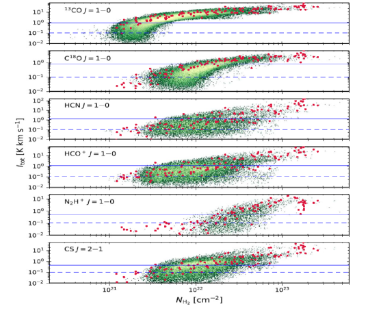
Figure 14: Comparison between the Orion A sampling observations and the mapping data of Yun et al. (2021). The figure presents a scanned copy of Fig. 15 from Yun et al. (2021), with red circles representing the intensities derived from the sampling observations. The solid blue line represents the approximate $3\sigma$ limit of the mapping data calculated using the velocity range of integration given by Yun et al. (2021) in their Table 2 and the rms noise in the spectra given in their Fig. 8. The dashed line represents the equivalent limit for the sampling data. See the main text for further details.

Paper I presented a comparison between the Perseus ¹²CO(1–0) and ¹³CO(1–0) sampling data and the mapping observations of the same lines by Ridge et al. (2006) using the FCRAO 14 m telescope. This comparison showed that sampling observations can reproduce at the 25% level both the mean intensity and the intensity dispersion as a function of $N$(H₂) derived from the mapping observations (Paper I, Sect. 4.1). For the Orion A cloud, Yun et al. (2021) have recently presented maps of several 3 mm emission lines carried out with the twin TRAO 14 m telescope, and this new data set provides an excellent opportunity to test again the ability of the sampling method to reproduce the global emission of a molecular cloud. The observations of Yun et al. (2021) consist of maps in the lines of ¹³CO(1–0), C¹⁸O(1–0), HCN(1–0), CS(2–1), HCO⁺(1–0), and N₂H⁺(1–0) that cover almost the full extent of the Orion A cloud emission (see the coverage in their Fig. 1). In contrast with the data from Ridge et al. (2006), the Yun et al. (2021) data are not publicly available, so our comparison with the Orion A data has been made by superposing our intensity distributions over those presented by Yun et al. (2021) in their Fig. 15. Since Yun et al. (2021) presented their intensities in $T_{\mathrm{A}}^{*}$ units (Neal Evans, private communication), which correspond to about half the intensities in units of $T_{\mathrm{MB}}$ (see the beam efficiencies in their Table 1), to correctly simulate a line comparison in $T_{\mathrm{MB}}$ units (as done with the data from Ridge et al. 2006), we divided our main-beam intensities by a factor of 2. The results from the comparison are shown in Fig. 14, which presents a superposition of our scaled-down intensities (red circles) over the intensities presented by Yun et al. (2021) in their Fig. 15.

As can be seen in Fig. 14, our sampling data match well the distribution of intensity as a function of $N$(H₂) derived from the mapping data for all observed lines. The best agreement is seen in the ¹³CO(1–0) data since this line presents the highest signal to noise, and its distribution can be reliably followed over two orders of magnitude in $N$(H₂). The intensity of the other lines cannot be followed over such a large range of column densities, but in all cases, the sampling data overlap well with the distribution of mapping intensities and presents a similar level of dispersion over the range of column densities for which the mapping data can be considered complete (over the blue solid line). Given the results in Fig. 14, we conclude that the sampling observations provide a good approximation to the distribution of intensities with $N$(H₂) found by mapping, and that they do not seem to miss any particular regime of intensities that is present in the maps.

A more quantitative comparison between our sampling data and the mapping observations of Yun et al. (2021) could be carried out using line luminosities. As discussed in our Sect. 3.7, line luminosities can be easily estimated from the sampling data by multiplying the observed line intensities by the surface area of the different column density bins, and luminosity estimates for the main transitions observed in our three target clouds are presented in Table. 6. Yun et al. (2021) have also calculated luminosities for the lines observed in their survey, but unfortunately the values given by these authors in their Sect. 5.4 suffer from several inaccuracies that make it necessary a revision (Neal Evans, private communication). A preliminary comparison with the revised luminosities of ¹³CO(1–0) and C¹⁸O(1–0) suggests a level of agreement with our sampling results at better than the 50% level, which is similar to the agreement found in Sect. 3.7 when comparing our luminosities with other estimates in the literature. A definitive comparison between our values and those of Yun et al. (2021) awaits the final estimate of the revised luminosities by these authors.

Appendix D Temperature effects

D.1 Gas temperature estimates

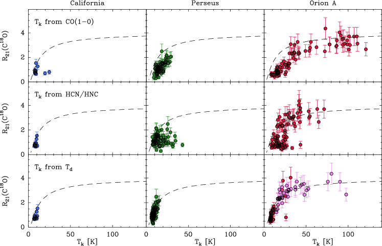
Figure 15: C¹⁸O(2–1)/C¹⁸O(1–0) intensity ratio as a function of the gas temperature determined using three different methods: peak of the ¹²CO(1–0) line (top), HCN(1–0)/HNC(1–0) line ratio method of Hacar et al. (2020) (middle), and the empirical fit based on the dust temperature described in the text (bottom). The data are color-coded as in Fig. 1, and the purple points in the bottom-right panel indicate the Orion A positions where the NH₃-based temperature estimate of Friesen et al. (2017) has been used. The dashed lines represent the expected line ratio under optically thin LTE conditions, and the ability of the data to match this curve reflects the quality of the temperature determination.

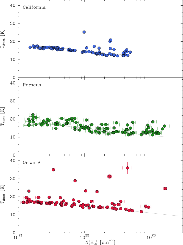
Figure 16: Distribution of dust temperature as a function of H₂ column density for the sampled positions of California, Perseus, and the regions of Orion A for which no NH₃-based gas temperature is available. The gray line represents the simple analytic fit to the equilibrium dust temperature described in the text. Dust temperature data are from Lada et al. (2017, California), Zari et al. (2016, Perseus), and Lombardi et al. (2014, Orion A).

To investigate the effect of temperature in the emission of the different lines, we first needed to determine its mean value along each observed line of sight. The ideal tool for this is a tracer that is bright enough to be detected at all column densities, has an excitation close to the gas kinetic temperature, and is optically thin so it samples the entire column density of gas at each position. The tracer in our data set that best approaches these characteristics is C¹⁸O, and in Paper I we used the C¹⁸O(2–1)/C¹⁸O(1–0) ratio to determine that the temperature in the Perseus positions is approximately constant at about 11 K, in agreement with previous ammonia results (Rosolowsky et al. 2008). While a similar analysis could be done with the Orion A data, our C¹⁸O(2–1) observations of California were limited to 13 positions (out of 80) due to observing-time constraints. As a result, it is not possible to derive a C¹⁸O line ratio over most of this cloud, and an alternative temperature determination is needed. In this appendix we explore three possible methods and judge their merit testing them against the C¹⁸O line ratio, which we consider the best available temperature indicator.

Our first (and simplest) temperature estimator is the peak intensity of the ¹²CO(1–0) line. ¹²CO is easily thermalized, and the $J$=1–0 line is optically thick. Under these conditions, the gas kinetic temperature $T_{\mathrm{k}}$ can be assumed to equal the excitation temperature, which is given by

$$T_{\mathrm{ex}}=\frac{h\nu/k}{\ln[1+\frac{h\nu/k}{T_{\mathrm{B}}-J_{\nu}(T_{\mathrm{bg}})}]},$$ (8)

where $\nu$ is the line frequency, $J_{\nu}$ the radiation temperature, and $T_{\mathrm{b}g}$ the cosmic background temperature (=2.73 K). To determine the ¹²CO(1–0) peak brightness temperature at each position, we fitted each spectrum using a Gaussian profile. This type of profile does not always represent the best fit to the complex ¹²CO(1–0) spectrum, but a visual inspection of the fits shows that the method provides a good approximation to the line peak. Using this estimate and Eq. D.1, we determined a ¹²CO(1–0)-based kinetic temperature at each cloud position in out sample. The top panel of Fig. 15 presents the C¹⁸O(2–1)/C¹⁸O(1–0) line ratio derived from our available data as a function of the gas temperature estimated using the ¹²CO(1–0) peak temperature. As can be seen, the line ratios for Perseus and Orion A systematically lie to the right of the dashed line, which corresponds to the prediction for the optically thin local thermodynamic equilibrium (LTE) conditions expected to apply. This systematic shift indicates that the ¹²CO(1–0) peak method overestimates the value of the C¹⁸O-inferred gas kinetic temperature by a significant margin. A similar overestimate of the gas temperature by the ¹²CO data was first noticed by Castets et al. (1990) in their multiline CO study of Orion A, and recent discussions of this effect have been presented by Hacar et al. (2020) and Roueff et al. (2021). The most likely cause of this overestimate is the high optical depth of the ¹²CO(1–0) line, which makes the emission originate from the cloud outer layers. These layers are exposed to the external UV radiation field and therefore warmer than the attenuated interior (e.g., Castets et al. 1990). A comparison of the CO-derived temperatures in Orion A with the NH₃-based temperature estimates of Friesen et al. (2017) supports this interpretation, and suggests that the ¹²CO data can overestimate the internal gas temperature by up to a factor of 2.

An alternative method for estimating the gas kinetic temperature is to use the HCN(1–0)/HNC(1–0) line ratio, which behaves as a chemical thermometer due to the high sensitivity to temperature of the relative abundance of the two HCN isomers (Hacar et al. 2020). Using NH₃ data from the Orion A cloud, Hacar et al. (2020) have calibrated the relation between gas temperature and HCN/HNC ratio, and proposed a simple prescription to derive the gas kinetic temperature (their Eqs. 3 and 4). We applied this prescription to our survey data, and determined a gas temperature at each observed position. In the middle row of panels of Fig. 15 we present the C¹⁸O(2–1)/C¹⁸O(1–0) line ratio as a function of the gas temperature estimated using the HCN/HNC line method. As can be seen, the Orion A data follow more closely the optically thin LTE limit line than when using the ¹²CO(1–0) line method, although this may simply reflect the fact that the HCN/HNC ratio was calibrated using NH₃ data from this cloud. In contrast, the HCN/HNC ratio method does not align well the Perseus line ratios with the analytic curve, indicating that the method does not provide a reliable estimate of the gas kinetic temperature in this cloud. This should have been expected since the HCN/HNC ratio method loses accuracy for temperatures below 15 K (Hacar et al. 2020).

As a third alternative to estimate gas temperatures, we explored the use of the dust temperature as a reference. Dust temperatures are derived together with H₂ column densities in the analysis of the Herschel data (Lombardi et al. 2014; Zari et al. 2016; Lada et al. 2017), so they are available at each cloud position. While the gas and dust components are only thermally coupled at densities in excess of $\approx 10^{4}$ cm^-3 (Goldsmith 2001), the dust temperature can still serve as an indicator of the presence (or absence) of energetic perturbations that may affect the gas temperature. In our clouds, the largest temperature perturbation occurs in Orion A, where the gas and dust in the vicinity of the ONC are heated by the newly formed stars. Since this temperature perturbation can be accurately characterized using the NH₃-derived temperatures of (Friesen et al. 2017), we used the NH₃ temperatures for the ONC vicinity, and used the dust temperature method only in the remaining parts of the clouds. In these parts, the temperature excursions are likely very small, as suggested by the dust temperature profiles shown in Fig. 16. These profiles indicate that the distribution of dust temperature in the three clouds has little dispersion, and that most values cluster along a well-defined band that runs almost horizontally. This band likely traces the equilibrium temperature of the dust for unperturbed cloud conditions since is very similar in the three clouds despite their significant differences in star-formation activity. It presents a slight decrease as $N$(H₂) increases that likely results from the inward attenuation of the interstellar radiation field, which is the main heating agent of the dust (Evans et al. 2001; Planck Collaboration et al. 2011). Following work by Hacar et al. (2017b) and Hocuk et al. (2017), we fitted the trend in the three clouds using the expression $T_{\mathrm{dust}}=19.0-4.0\log_{10}(N(\mathrm{H}_{2})/10^{21}\,\mathrm{cm}^{-2})$ (gray line in the figure).

To use the dust temperature as a proxy for the gas temperature, we followed a simple empirical approach. We first subtracted from the dust temperature the observed gradient with $N$(H₂) since this gradient is caused by the attenuation of the interstellar radiation field, and is not expected to affect the gas component because is heated by cosmic rays and not thermally coupled to the dust in the outer cloud (Goldsmith 2001; Galli et al. 2002). To the result, we simply added a global offset of 8 K, which has been derived from an empirical match to the C¹⁸O(2–1)/C¹⁸O(1–0) line ratio. As seen in the bottom row of panels in Fig. 15, the empirical dust fit, when complemented with the NH₃-derived temperatures of Friesen et al. (2017), provides a better match to the C¹⁸O(2–1)/C¹⁸O(1–0) line ratio than the fits obtained using either the CO(1–0) peak intensity or the HCN/HNC line ratio. For this reason, we used this fit as the temperature indicator in the three clouds of our sample. Further work is needed to understand the correct level of coupling between the gas and dust temperatures through the clouds.

D.2 Temperature-correction factors

To determine (and possibly correct for) the effect of temperature variations in the emission profile of the different clouds, we needed to determine how the intensity of any line depends on the gas kinetic temperature. This determination requires a certain degree of approximation because the intensity of a line depends on a complex combination of the physical and chemical conditions of the emitting cloud, which are in principle not well known. The observed systematic behavior of the line intensities, however, suggests that the main characteristics of the emission are dominated by relatively few cloud properties that could be approximated using a simplified model. If this is the case, we could define a series of correction factors that relate the intensity emitted by gas at an arbitrary temperature $T_{\mathrm{k}}$ with the emission that the same gas would emit if it were a reference temperature of 10 K. These factors are defined as

$$f_{10\mathrm{K}}(T_{\mathrm{k}})\equiv\frac{I\;(T_{\mathrm{k}})}{I\;(10\mathrm{\leavevmode\nobreak\ K})},$$ (9)

were $I(T_{\mathrm{k}})$ and $I(10\leavevmode\nobreak\ K)$ are the intensities at the two temperatures. To first approximation, we could use these factors to convert any observed line intensity into the expected intensity that the same line of sight would emit if it were at 10 K.

As a first step to understand the behavior of the correction factors, we considered two simple limiting cases. If the line is optically thick and thermalized ($T_{\mathrm{e}x}=T_{\mathrm{k}}$), which may be the case for a low $J$ ¹²CO transition, the equation of radiative transfer states that the integrated intensity will be equal to $(J_{\nu}(T_{\mathrm{k}})-J_{\nu}(T_{\mathrm{b}g}))\;\Delta\mathrm{V}$, where $J_{\nu}$ is the radiation temperature, $T_{\mathrm{b}g}$ is the cosmic background temperature, and $\Delta\mathrm{V}$ the linewidth in units of velocity. Under these conditions, the correction factor defined as the line intensity at an arbitrary kinetic temperature divided by the intensity at 10 K will be

$$f^{\mathrm{t}hick}_{10\mathrm{K}}(T_{\mathrm{k}})=\frac{J_{\nu}(T_{\mathrm{k}})-J_{\nu}(T_{\mathrm{b}g})}{J_{\nu}(10\leavevmode\nobreak\ \mathrm{K})-J_{\nu}(T_{\mathrm{b}g})}.$$ (10)

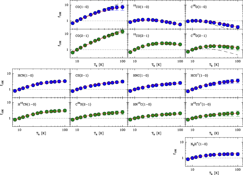
Figure 17: Intensity predictions of the observed lines as a function of gas temperature normalized to their value at 10 K. The intensities have been calculated by running the model of the Perseus cloud presented in Paper I for 12 different gas temperatures. For each temperature, six different H₂ column densities in the range $2\times 10^{21}$ to $2\times 10^{23}$ cm^-2 have been assumed, and each circle represents the intensity average with an error bar that indicates the 1$\sigma$ dispersion (and is often smaller than the marker size). The upper block of panels contains the CO isotopologs, the middle block contains the traditional dense-gas tracers and their isotopologs, and the bottom panel contains N₂H⁺(1–0). The solid red lines represent the empirical fits described in the text and used in the analysis to correct for gas temperature variations. The dashed black lines in the CO and C¹⁸O panels represent the optically thick and thin LTE solutions discussed in the text.

Another simple illustrative case is the optically thin line of a species in LTE, in which the excitation temperature of all transitions equals the kinetic temperature. For this case, which may be applicable to the C¹⁸O lines, the integrated intensity will be $[J_{\nu}(T_{\mathrm{k}})-J_{\nu}(T_{\mathrm{b}g})]\;\tau_{\nu}\;\Delta\mathrm{V}$, where the optical depth $\tau_{\nu}$ is given by

$$\tau_{\nu}=\frac{c^{3}}{{8\pi\nu^{3}}}\;\frac{g_{\mathrm{u}}A_{\mathrm{ul}}N}{{\Delta V}}\;\frac{(1-e^{{-h\nu}/kT_{\mathrm{k}}})\;e^{-E_{\mathrm{l}}/kT_{\mathrm{k}}}}{Q(T_{\mathrm{k}})},$$ (11)

and where $g_{\mathrm{u}}$ is the statistical weight of the upper level, $A_{\mathrm{ul}}$ is the Einstein coefficient of spontaneous emission, $N$ the molecular column density, and $Q$ the partition function calculated as a sum over all relevant energy levels. As in the thick case, we can derive a correction factor by dividing the expected line intensity at any given temperature by the intensity at 10 K.

In real clouds, most molecular tracers are not thick and thermalized or thin and in LTE, so the conversion factors between temperatures will likely deviate from the previous two simple limits. To calculate these factors, we therefore had to solve the equation of radiative transfer under physical and chemical conditions that match those of real clouds. In Paper I, we presented a radiative transfer model of the Perseus cloud that was able to reproduce the intensity distribution of multiple lines (see Tables 3 and D.1 in Paper I ). This model used a simple parameterization of the gas physical and chemical conditions, and in particular, assumed a constant gas temperature of 11 K as indicated by previous ammonia estimates (Rosolowsky et al. 2008).

To model how the intensity of the different lines is expected to vary with the gas kinetic temperature, we reran the Perseus model for 12 different temperatures that cover the range 8-100 K. For each gas temperature, we estimated the emergent intensity of the different lines as a function of H₂ column density using six logarithmically spaced H₂ column densities that cover the range $2\times 10^{21}$-$2\times 10^{23}$ cm^-2. For each line, we normalized the intensity at any given temperature by the value at a reference temperature of 10 K as described in Equ. 9.

Figure 17 (top panels) shows the results from our radiative transfer model for the observed transitions of the CO isotopologs. The circles represent the intensity ratio averaged over the range of column densities covered by each model, and the error bars represent the corresponding dispersion. The red lines represent a set of analytic fits described below, and the black dashed lines represent the two previously described limits: the optically thick thermalized limit for ¹²CO and the optically thin LTE case for C¹⁸O. As can be seen, the model CO intensities approximately follow the optically thick prediction at low temperatures. As this parameter increases over about 50 K, however, the higher $J$ levels of CO become more populated and the optical depth of the lower transitions starts to drop, decreasing the match with the thick approximation. As also shown in the figure, the model C¹⁸O intensities follow the optically thin LTE limit at low temperatures, but as the temperature increases, the LTE approximation breaks down and the intensities deviate from the dashed line.

Model results for the intensity ratio of the traditional dense-gas tracers and their isotopologs are presented in the middle group of panels of Fig. 17, and the special case of N₂H⁺(1–0) is shown in the bottom panel. As can be seen, the optically thick lines from the main isotopologs present a higher sensitivity to the temperature increase, but the general behavior of both thick and thin lines is similar. It is characterized by an increase of the line ratio at low temperatures and a gradual flattening as the temperature exceeds 30-50 K.

We can summarize the results of our modeling by saying that the intensity of all the observed lines is expected to vary smoothly and systematically with the gas kinetic temperature in the range of interest (8-100 K). Our model results provide a simple recipe to quantify and, if necessary, correct for changes in the gas temperature across each cloud. Since our model results have been calculated for a discrete number of temperatures, it may be necessary to interpolate the corrections to the exact temperature value of each position. This could be done by interpolating the model results, but it seems more convenient to find analytic expressions that fit the model results and can be used to quickly compute correction factors for any gas temperature.

Inspired by the similar behavior of all the different dense-gas tracers, and by some of the factors that appear in the LTE equations, we explored the possibility of fitting the dense-gas tracer data using the simple expression

$$f_{10\mathrm{K}}(T_{\mathrm{k}})=\frac{\exp(-T_{0}/T_{\mathrm{k}})}{\exp(-T_{0}/10\mathrm{\leavevmode\nobreak\ K})},$$ (12)

where $T_{0}$ is a reference temperature that has been determined by fitting the data in Fig. 17. The fit results are represented with red lines in the figure, and the $T_{0}$ values for each dense gas transition are given in Table 10. As can be seen, a simple exponential factor provides a reasonable fit to all dense-gas tracer lines and requires $T_{0}$ values in the narrow range 7-13 K.

Fitting the intensity ratios of the CO isotopologs requires more complex expressions because the model results present a diversity of behaviors that range from the quasi-linear increase of the thick main isotopologs to the systematic decrease of the C¹⁸O lines. Using again the LTE formulas as an inspiration, and favoring the use of similar factors for similar lines, we have found that it is possible to fit the model results using an expression of the form

$$f_{10\mathrm{K}}(T_{\mathrm{k}})=\frac{g_{1}(T_{\mathrm{k}})}{g_{1}(10\mathrm{\leavevmode\nobreak\ K})}\times\frac{g_{2}(T_{\mathrm{k}})}{g_{2}(10\mathrm{\leavevmode\nobreak\ K})},$$ (13)

where $g_{1}(T_{\mathrm{k}})$ and $g_{2}(T_{\mathrm{k}})$ are the empirical functions given in Table 11. As can be seen in Fig. 17, this factorization provides a reasonable fit to intensity correction factors of all CO isotopologs in the 8-100 K range. While convenient, these expressions only represent empirical fits to the model results, and do not have any underlying theoretical basis.

Table 10: Reference T₀ temperature for dense-gas tracers.

Line	$T_{0}$ [K]	Line	$T_{0}$ [K]
HCN(1–0)	13	H13CN(1–0)	12
CS(2–1)	12	C34S(2–1)	9
HNC(1–0)	10	HN13C(1–0)	7
HCO+(1–0)	13	H13CO+(1–0)	8
N2H+(1–0)	7

Table 11: Temperature correction factors for CO isotopologs.

Line	$g_{1}(T_{\mathrm{k}})$	$g_{2}(T_{\mathrm{k}})$		$g_{1}(T_{\mathrm{k}})$	$g_{2}(T_{\mathrm{k}})$
CO(1-0)	$T_{\mathrm{k}}^{1.3}$	$(1-e^{-50/T_{\mathrm{k}}})$	CO(2-1)	$T_{\mathrm{k}}^{1.4}$	$(1-e^{-80/T_{\mathrm{k}}})$
13CO(1-0)	$e^{-4/T_{\mathrm{k}}}$	$(1-e^{-50/T_{\mathrm{k}}})$	13CO(2-1)	$e^{-14/T_{\mathrm{k}}}$	$(1-e^{-80/T_{\mathrm{k}}})$
C18O(1-0)	1	$(1-e^{-50/T_{\mathrm{k}}})$	C18O(2-1)	$e^{-10/T_{\mathrm{k}}}$	$(1-e^{-80/T_{\mathrm{k}}})$

Appendix E Plots of isotopic ratios

Figs. 18 and 19 present intensity ratios as a function of H₂ column density for the rare CO isotopologs and the traditional dense-gas tracers. A comparison with the standard isotopic value (represented with a dashed line) indicates that the emission from the rare CO isotopologs is optically thin, while the emission from the dense-gas tracers is optically thick.

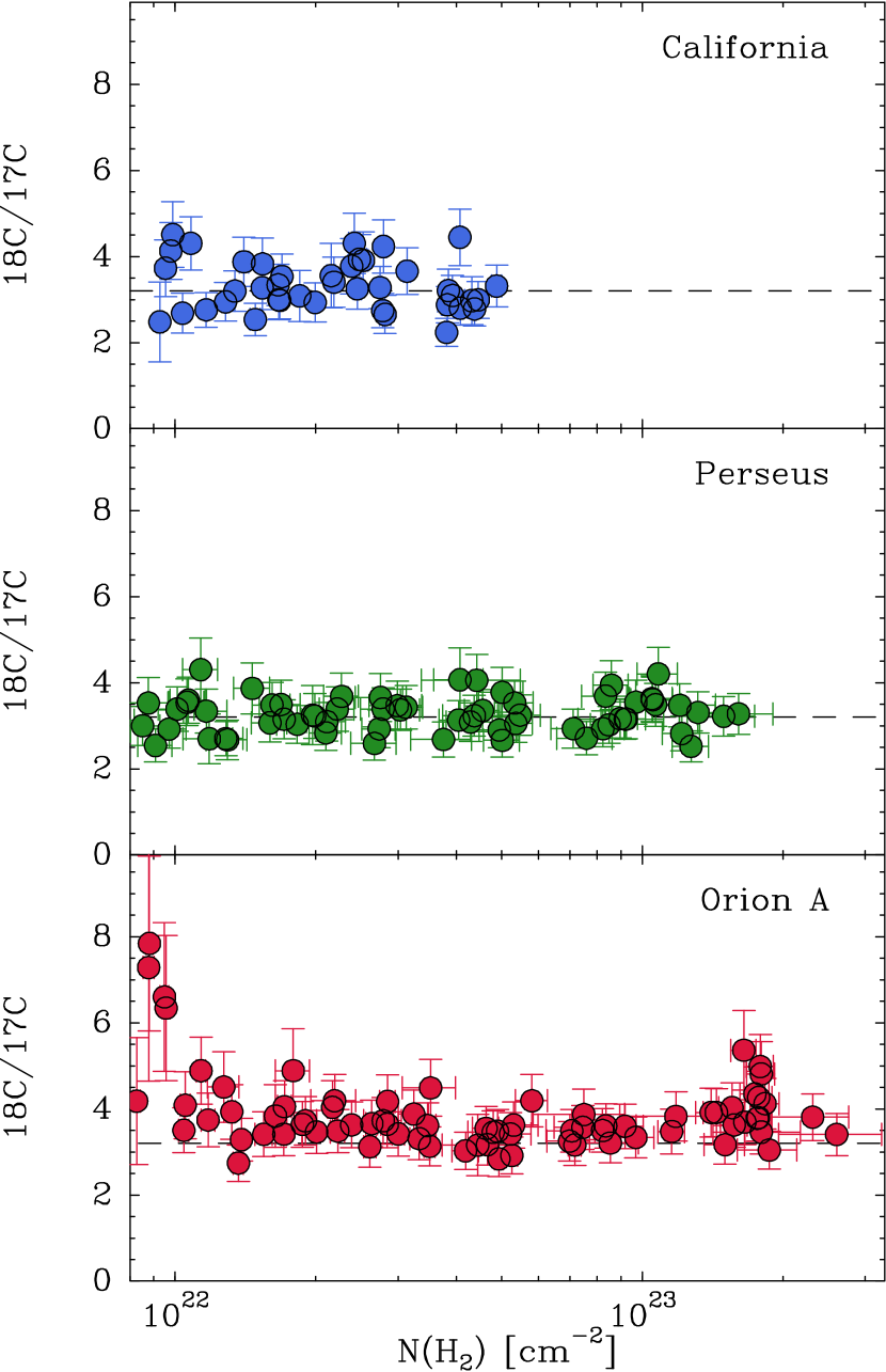
Figure 18: C¹⁸O(1–0)/C¹⁷O(1–0) intensity ratio as a function of the H₂ column density used to determine the optical depth of the rare isotopologs. The dashed horizontal line represents the standard isotopic ratio of 3.2 (Wilson & Rood 1994), and the good match with the observations indicates that both transitions are optically thin in all three clouds. Note the restricted range of the x-axis due to the low S/N of the line ratio for very low values of $N$(H₂).

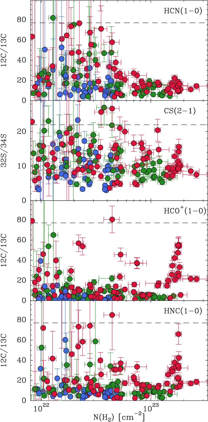
Figure 19: Isotopic intensity ratios for the traditional dense-gas tracers as a function of H₂ column density for California, Perseus, and Orion A. The $N$(H₂) range has been reduced compared to other plots due to the low signal-to-noise ratio of the data with low $N$(H₂). The dashed horizontal lines represent the standard interstellar medium isotopic ratios (77 for ¹²C/¹³C and 22 for ³²S/³⁴S), and the low value of the observed ratios indicates that the emission of the main isotopolog is optically thick. Note how the outflow points from Orion A (near $2\times 10^{23}$ cm^-2) have lower optical depths in some tracers but are still optically thick. No temperature correction has been applied to the data.

Appendix F Luminosities from mapping and sampling methods

Table 12 presents the set of luminosity values used in the comparison between sampling and mapping luminosities shown in Fig. 6. The luminosities from mapping observations were chosen from the literature requiring that they were well documented and reliable calibrated, or that the mapping data were publicly available so that the luminosities could be independently estimated. If necessary, luminosities have been re-scaled to the Gaia-based distances of Zucker et al. (2019) given in Sect. 1. To compare with the Perseus estimates from Ridge et al. (2006) and the Orion A estimates from Nishimura et al. (2015), we restricted our sampling estimates to the same cloud area not masked by these authors, for which we used their publicly available data. A full discussion of the luminosity comparison is given in Sect. 3.7.

Table 12: Line luminosities from mapping and sampling measurements.

Line	$L_{\mathrm{sampling}}$	$L_{\mathrm{mapping}}$	Map ref.
	(K km s-1 pc2)	(K km s-1 pc2)
Orion A
12CO(1–0)	28,200	21,300	Lew22
12CO(2–1)	19,100	16,000	Nis15
13CO(2–1)	3,350	2,030	Nis15
C18O(2–1)	91	53	Nis15
Perseus
12CO(1–0)	3,890	3,920	Rid06
12CO(1–0)	6,900	8,530	Lew22
13CO(1–0)	700	810	Rid06
HCN(1-0)	77	67	Dam23
California
12CO(1–0)	35,200	30,500	Lew22