Characterising ultra-high-redshift dark matter halo demographics and assembly histories with the gureft simulations

Abstract

Dark matter halo demographics and assembly histories are a manifestation of cosmological structure formation and have profound implications for the formation and evolution of galaxies. In particular, merger trees provide fundamental input for several modelling techniques, such as semi-analytic models (SAMs), sub-halo abundance matching (SHAM), and decorated halo occupation distribution models (HODs). Motivated by the new ultra-high-redshift ($z\gtrsim 10$) frontier enabled by JWST, we present a new suite of Gadget at Ultrahigh Redshift with Extra-Fine Timesteps (gureft) dark matter-only cosmological simulations that are carefully designed to capture halo merger histories and structural properties in the ultra-$z$ universe. The simulation suite consists of four $1024^{3}$-particle simulations with box sizes of $5$, $15$, $35$, and $90$ Mpc h^-1, each with 170 snapshots stored between $40\geq z\geq 6$. With the unprecedented number of available snapshots and strategically chosen dynamic range covered by these boxes, gureft uncovers the emerging dark matter halo populations and their assembly histories in the earliest epochs of cosmic history. In this work, we present the halo mass functions between $z\sim 20$ to 6 down to $\log(M_{\text{vir}}/\text{M}_{\odot})\sim 5$, and show that at high redshift, these robust halo mass functions can differ substantially from commonly used analytic approximations or older fitting functions in the literature. We also present key physical properties of the ultra-high $z$ halo population, such as concentration and spin, as well as their mass growth and merger rates, and again provide updated fitting functions.

1 Introduction

Dark matter accounts for the bulk of the matter budget in our Universe and it is the fundamental driver of structure formation across a vast range of scales, from the typical length scales where matter becomes virialized (e.g. a few kilo-parsecs, White & Frenk 1991) to the cosmic web structures (e.g. tens of mega-parsecs, Peebles 1980). Halo structural properties can have strong implications for the properties of the galaxies that form within them. For example, halo spin and concentration can affect galaxy sizes and rotation velocities (Mo et al., 1998; Bullock et al., 2001b; Somerville et al., 2008b); halo circular velocity sets the depth of the potential well that gas must escape in order to be ejected by feedback processes, and concentration, density profile, and substructure tie closely to the number and distribution of satellite galaxies (Navarro et al., 1997). Understanding the evolution of the overall demographics of dark matter halos is key to interpreting the evolution of the number density, spatial distribution, and clustering of observed galaxies across cosmic time. In addition, the assembly and merger histories of dark matter halos also have strong impacts on the star formation histories of enclosed galaxies (e.g. Conselice et al., 2003) and the growth of the supermassive black holes hosted in their nuclei (e.g. Hopkins et al., 2007). Overall, dark matter halos provide a fundamental basic framework for modelling and interpreting observed galaxy populations (see Wechsler & Tinker 2018 for a review).

Cosmic microwave background observations and galaxy surveys have provided strong evidence that our Universe is composed of mostly dark energy ($\Lambda$) and cold dark matter (CDM), and have provided fairly precise constraints on the fundamental cosmological parameters (e.g. Spergel et al., 2003; Planck Collaboration, 2014). This paradigm is commonly referred to as the $\Lambda$CDM model. Over the years, state-of-the-art dark matter-only cosmological simulations, such as Millennium (Springel et al., 2005), Millennium-II (Boylan-Kolchin et al., 2009), Bolshoi (Klypin et al., 2011), MultiDark and Bolshoi-Planck (Prada et al., 2012; Klypin et al., 2016), Uchuu (Ishiyama et al., 2021), Euclid Flagship (Potter et al., 2017), AEMULUS (DeRose et al., 2019), and AbacusSummit (Garrison et al., 2016; Maksimova et al., 2021), have been conducted to gain insights into the formation of large-scale structures and the assembly history of halos under the paradigm of dark matter dominated hierarchical structure formation. $\Lambda$CDM-based cosmological-scale hydrodynamic and $N$-body simulations incorporating baryonic physics have been shown to be quite successful at reproducing many observed properties of galaxies across cosmic time (for reviews see Somerville & Davé, 2015; Naab & Ostriker, 2017). Furthermore, simulated halo populations from this standard cosmological framework have also been extensively used to build galaxy models with semi-analytic (e.g. galform (Cole et al., 2000), L-Galaxies (Henriques et al., 2015), SAGE (Croton et al., 2016), Galacticus (Benson, 2010), Delphi (Dayal et al., 2014; Dayal et al., 2019), Santa Cruz SAM (Somerville et al., 2008a; Somerville et al., 2015)) and (semi-)empirical modelling techniques (e.g. UniverseMachine (Behroozi et al., 2019; Behroozi et al., 2020), DREaM (Drakos et al., 2022), Trinity (Zhang et al., 2023), Emerge (Moster et al., 2018; O’Leary et al., 2023)).

In particular, dark matter halo merger and assembly histories, also commonly referred to as merger trees, are the backbone for semi-analytic models for galaxy formation and evolution (for reviews see Baugh et al., 2006; Benson, 2010; Somerville & Davé, 2015). These merger trees can either be extracted from $N$-body simulations (Behroozi et al., 2013b; Rodriguez-Gomez et al., 2015; Elahi et al., 2019) or constructed with a probabilistic, Monte Carlo approach (Lacey & Cole, 1994; Somerville & Kolatt, 1999; Somerville et al., 2008a; Parkinson et al., 2008; Jiang & van den Bosch, 2014) based on the Extended Press-Schechter (EPS) formalism (Press & Schechter, 1974; Bond et al., 1991; Lacey & Cole, 1993). At lower redshifts ($z\lesssim 6$), it has been shown that the predictions of semi-analytic models run within EPS trees differ from those run within $N$-body trees at a level that is within the uncertainties on the parameters of the baryonic physics models; i.e., the differences in the key predictions are relatively small, and can be largely removed by re-calibrating the model parameters (see e.g. Gabrielpillai et al., 2022). However, Yung et al. (2023a) showed that the SAM results based on EPS trees can diverge significantly from those using $N$-body trees at $z\gtrsim 10$, especially in massive halos. We also note that it is difficult to directly assess the performance of EPS merger trees at high- to- ultra-high redshift (e.g. $z\gtrsim 10$) as the typical number of snapshots available and mass range covered by currently available N-body simulations are not optimised for the ultra-high-redshift universe.

The new frontier in the observable universe enabled by JWST presents new challenges and needs for galaxy formation simulations and theory. Numerical simulations inevitably face limitations from the tension between simulated volume and mass resolution, limited by the number of particles or grid cells that can be held in the memory of the largest available computers. A large simulated volume is essential to capture the large-scale spatial distribution of structures, as well as providing robust statistical samples for rare objects. On the other hand, high mass resolution is required to properly resolve both the low-mass halo populations and the progenitors of the massive halos. Current state-of-the-art cosmological simulations cover volume and mass resolutions that are sub-optimal for tracking the assembly history of halos in the high (e.g. $z\gtrsim 10$) to ultrahigh (e.g. $z\gtrsim 15$) redshift universe. While some of the latest cosmological simulations are reaching large volumes and dynamic range (e.g. Uchuu (Ishiyama et al., 2021), MilleniumTNG (Pakmor et al., 2022)) thanks to the fast-growing capabilities of computing facilities, it is often impractical to overcome this bottleneck with brute force as the tension becomes even more pronounced in the early universe, as the emerging halo populations are expected to be orders of magnitude rarer and lower mass than their low-redshift counterparts. In addition, the typical number of high- and ultra-$z$ snapshots stored by large cosmological simulations are sparse and insufficient for reconstructing halo merger histories, as the cost for storage is also a major limiting factor.

In light of the above considerations, we introduce a new suite of dark matter-only, cosmological simulations designed to collectively address this dynamic range problem. This work provides simulated halo mass functions and halo structural properties across a wide mass range as well as high temporal resolution halo merger trees to aid galaxy formation modelling in this new era. These simulations are extremely timely for the interpretation of recent JWST observations of the ultra-high redshift universe. With the first year of scientific operations, JWST has already revealed surprising and exciting results about the early universe. Early Release Observations (ERO) and Early Release Science (ERS) observations such as SMACS0723, GLASS, and CEERS almost immediately yielded galaxy candidates that broke existing redshift records, pushing into the $z\gtrsim 10$ regime (e.g. Finkelstein et al., 2022, 2023; Naidu et al., 2022; Castellano et al., 2022; Atek et al., 2022; Adams et al., 2022; Donnan et al., 2022; Harikane et al., 2023b). This progress has continued rapidly with additional surveys such as NGDEEP (Bagley et al., 2023; Leung et al., 2023) and JADES (Curtis-Lake et al., 2022; Robertson et al., 2023), and with spectroscopic confirmation of many of the $z\gtrsim 10$ candidates (Arrabal Haro et al., 2023; Fujimoto et al., 2023; Harikane et al., 2023a). JWST has also revealed that there are a surprising number of obscured active galactic nuclei (AGN) and accreting supermassive black holes (SMBH) in the very early universe (e.g. Kocevski et al., 2023b, a; Yang et al., 2023; Barro et al., 2023; Larson et al., 2023).

The results presented in this work serve as a fundamental building block for the next generation of semi-analytic models for galaxies and black holes at ultra-high-redshift. The predictions of the Santa Cruz SAM with the current configuration and calibrations (Gabrielpillai et al., 2022) at ultra-high redshifts (e.g. $8\lesssim z\lesssim 17$) are presented in Yung et al. (2023a). In a series of planned works, we will explore the impact of a wide variety of physical processes that operate in the ultra-high-$z$ universe, such as black hole seeding and growth, on the formation and evolution of galaxies across cosmic time. In the same spirit as the Semi-analytic forecasts for the Universe series (Yung et al., 2019, 2022, 2023b), we will also explore the co-evolution of early supermassive black holes and their host galaxies via various feedback channels, and present predictions and forecasts for current and future telescopes (Yung et al., 2021b; Yung et al., 2021a). Additionally, the gureft suite is being used to develop machine learning based techniques to very rapidly generate accurate halo merger histories over a large dynamic range in mass and redshift (Nguyen et al., 2023).

The structure of this paper is as follows: the design and specifications of the gureft simulation suite are presented in Section 2. We then the halo mass functions and key present key physical properties of the simulated halo populations in Section 3. We discuss our results in Section 4, and provide a summary and conclusions in Section 5.

Table 1: Specifications of the gureft simulation suite and the Bolshoi-P and SMDPL simulations from the MultiDark suite.

	Box size	$M_{\text{DM}}$	N	$\epsilon$
	[Mpc $h^{-1}$]	[M⊙ $h^{-1}$]		[kpc $h^{-1}$]
gureft-05	5	$9.92\times 10^{3}$	$1024^{3}$	0.16
gureft-15	15	$2.68\times 10^{5}$	$1024^{3}$	0.49
gureft-35	35	$3.40\times 10^{6}$	$1024^{3}$	1.14
gureft-90	90	$5.78\times 10^{7}$	$1024^{3}$	2.93
BolshoiP	250	$1.55\times 10^{8}$	$2048^{3}$	1.0
SMDPL	400	$9.63\times 10^{7}$	$3840^{3}$	1.5
VSMDPL	160	$6.20\times 10^{6}$	$3840^{3}$	2.0

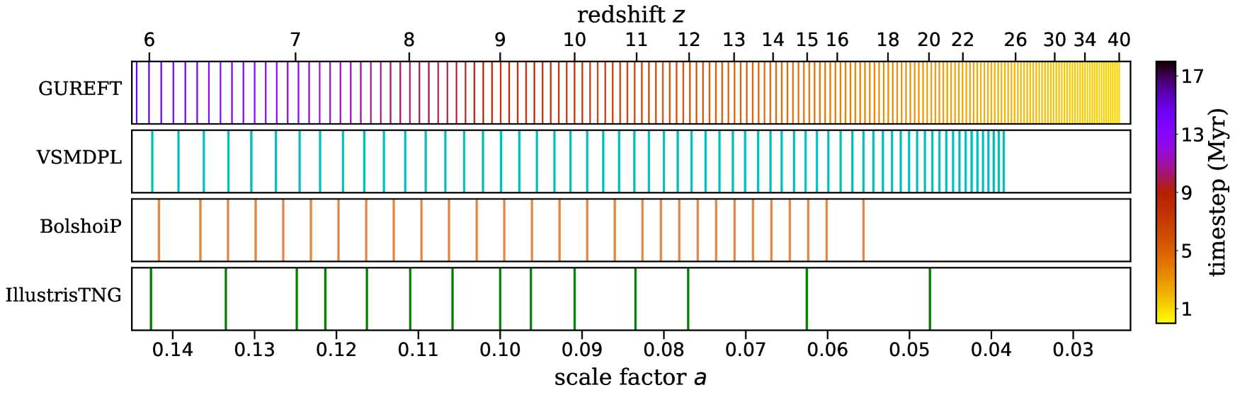
Figure 1: This figure shows the redshifts and scale factors where snapshots are stored for the gureft simulations (top), which may be compared to same quantities for the vsmdpl (second row), Bolshoi-Planck (third row), and IllustrisTNG (bottom) simulations over the same redshift range. For the gureft simulations, we colour-coded the lines by the time elapsed between snapshots. Many previous $N$-body simulations have stored only a sparse number of snapshots at high redshifts.

2 The GUREFT simulation suite

The gadget at Ultrahigh Redshift with Extra-Fine Timesteps (gureft; pronounced graft) is a suite of cosmological simulations designed to resolve the merger and assembly history of dark matter halos emerging in the early Universe. Throughout this work, we adopt cosmological parameters $\Omega_{\text{m}}=0.307$, $\Omega_{\Lambda}=0.693$, $H_{0}=67.8$ km s^-1 Mpc^-1, $\sigma_{8}=0.829$, and $n_{s}=0.960$; which are broadly consistent with the constraints reported by the Planck Collaboration (Planck Collaboration XIII 2016). These are identical to the cosmological parameters adopted in the Bolshoi-Planck (Klypin et al., 2016, hereafter BolshoiP), and Small and Very Small Multidark (SMDPL and VSMDPL; see also Klypin et al., 2016) simulations, which we use as a comparison and complement throughout this work.

The gureft suite consists of four dark matter-only $N$-body simulations carried out with the publicly available version of gadget-2 code (Springel, 2005). The nested grid initial conditions for our high-resolution simulations are generated using the Multi-Scale Initial Conditions (MUSIC; Hahn & Abel, 2011) at $z_{\text{init}}=200$ using the second-order Lagrangian perturbation theory (2LPT), which is more accurate than the Zel’dovich approximation (Scoccimarro, 1998; Crocce et al., 2006). In a set of pilot simulations, we carried out a convergence test with initial redshifts at $z_{\text{init}}=100$, 200, and 400, and find no noticeable effects on the output halo population at $z<40$.

Our suite of four simulations each consists of $N=1024^{3}$ DM particles, representing matter distributed across simulated volumes with 5, 15, 35, and 90 Mpc $h^{-1}$ on a side. These simulations are labelled gureft-05, gureft-15, gureft-35, gureft-90 accordingly. The specifications of these simulations are summarised in Table 1, along with the corresponding specifications for BolshoiP, SMDPL, and VSMDPL. We report on the size of the simulated volume, mass of DM particle ($M_{\text{DM}}$), number of particles, and the gravity softening length ($\epsilon$). The redshifts of the output snapshots and the rationale for the chosen box sizes are further detailed in Sections 2.1 and 2.2.

Halos are identified with the six-dimensional phase-space halo finder rockstar and a gravitationally consistent merger tree construction algorithm consistent trees (Behroozi et al., 2013a; Behroozi et al., 2013b). We adopted the Bryan & Norman (1998) virial mass definition and require at least 100 DM particles for a halo to be considered resolved. The rockstar type approach is more robust at high redshift compared to the commonly used alternative "friends-of-friends" based halo finding algorithm, which tends to spuriously group halos in elongated (filamentary) structures together (Klypin et al., 2011).

2.1 Spacing of Output Snapshots

The temporal resolution of merger trees (which is limited by the spacing between output snapshots from $N$-body simulations) remains a major limitation in reconstructing ultra high-$z$ merger histories from simulation outputs. Most previous large volume $N$-body simulations have stored sparsely spaced snapshots at high redshifts (e.g. $z>8$) and increased the number of snapshots stored towards lower redshifts (e.g. $z<3$), as demonstrated in Fig. 1.

For the gureft simulations, to ensure that we properly resolve the formation history of halos out to $z\sim 20$, we chose a spacing between snapshots of one-tenth of the halo dynamical time at the output redshift, and store a total of 171 snapshots between $z\sim 40$ to 6. The redshifts and scale factors of stored snapshots are shown in Fig. 1. We also show snapshots available from Bolshoi-Plank and IllustrisTNG in the same redshift range for comparison. The more finely spaced snapshots of gureft allow for the reconstruction of detailed merger histories out to ultra high redshifts.

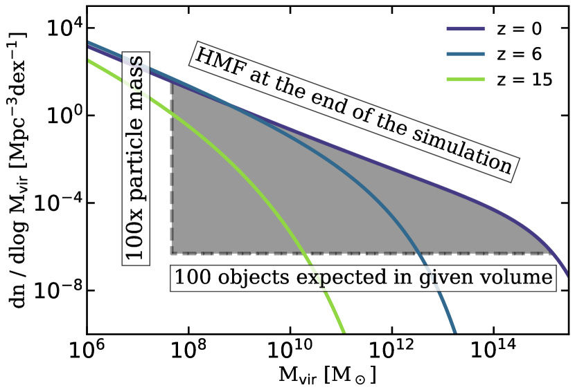
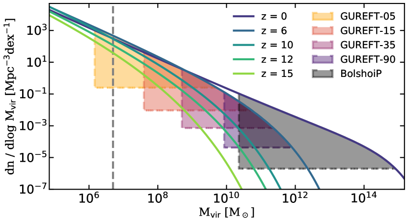
Figure 2: This figure shows “coverage triangles” that illustrate the rationale for choosing the mass resolution and volume of the gureft suite. In the left panel, we show an example ‘coverage triangle’ in the virial mass-number density space, which highlights the mass range of halos that are expected to be resolved by a cosmological simulation over time. The left boundary of this triangle is the mass where halos are well-resolved for the simulation $M_{\text{vir}}=100M_{\text{DM}}$ (opposite). The lower bound is where 100 objects are expected for the simulated volume, and the upper bound is the expected number density of halos at the redshift of the final output of the simulation. Objects to the left of the triangle fall below the mass resolution of the simulation and those below the triangle are too rare to be found in large numbers in the simulated volume. In the right panel, we show colour-coded coverage triangles for the suite of gureft simulations (which terminate at $z=6$) and Bolshoi-Planck (which terminates at $z\sim 0$). The vertical line marks the atomic cooling limit, below which galaxy formation is expected to be inefficient. In both panels, we show HMFs at selected redshifts from past studies to qualitatively represent how the halo population evolve over time.

2.2 Box sizes and resolution

The box sizes and resolution of the four gureft simulations are selected to capture the assembly histories of halos across a wide mass range while providing an adequate sample size for statistical studies. In addition, the mass range covered by these boxes are designed to overlap with each other, which allows us to carry out convergence tests and to graft together the merger trees extracted from these simulations using machine learning approaches (Nguyen et al., 2023, T. Nguyen et al. in prep).

We introduce a set of ‘coverage triangles’ in the virial mass-number density space to illustrate the rationale for the choice of survey volume and corresponding mass resolution. In this work, we assume that halos with 100 particles are well-resolved (we test this assumption in subsequent sections), implying a mass threshold of $M_{\text{vir, res}}=100$ $M_{\text{DM}}$. The leftmost edge of the triangles in Fig. 2 show this limit for each of the simulation volumes. The horizontal line marks the number density which would yield at least 100 halos in the given volume. Given a fixed number of particles, the simulation volume is inversely related to its mass resolution. This restriction is reflected in the area of the triangles. The number of particles in a simulation is limited by the computational resources available and the efficiency of numerical methods. The hypotenuse of the coverage triangles marks the HMF at a particular epoch. In Fig. 2, we show HMFs at selected redshifts to illustrate how the mass distribution of halo populations evolves over cosmic time. We note that the HMFs shown here are based on fits to previous simulations, and are extrapolated in some regions. They are meant as a qualitative illustrations and are not necessarily highly accurate. For $z\leq 10$, we show the HMF fits from the MultiDark simulations (Rodríguez-Puebla et al., 2016; Rodríguez-Puebla et al., 2017) and at $z>10$ we show the HMFs fits presented in Yung et al. (2020), which are obtained by combining BolshoiP (Klypin et al., 2016) with very high resolution, small volume boxes from Visbal et al. (2018).

In the right panel of Fig. 2, we show the series of coverage triangles for the gureft simulations and BolshoiP. As illustrated, the suite of four simulations are designed to progressively increase in size as the mass resolution becomes coarser, with adequate overlap between boxes in the mass range where halos are both well-resolved and are present in sufficient numbers to comprise statistically robust samples. The goal of this configuration is to maximise coverage of the halo population that is most important for modelling galaxy and BH formation physics over this redshift interval. For example, gureft-05 is designed to resolve the low-mass halo populations (e.g. $6\lesssim\log(M_{\text{vir}}/\text{M}_{\odot})\lesssim 9$) between $18\gtrsim z\gtrsim 10$, which may host Population III stars and black hole seeds. More massive halos are covered with the adjacent box gureft-15, resolving halo masses $7.5\lesssim\log(M_{\text{vir}}/\text{M}_{\odot})\lesssim 11$ between $12\gtrsim z\gtrsim 6$, which reaches down to approximately the halo mass range where metal-free atomic cooling is efficient ($T_{\rm vir}\simeq 10^{4}$ K. Similarly, the gureft-35 and gureft-90 boxes contain the more massive halos that are likely to host galaxies that are observable with JWST (Yung et al., 2023b).

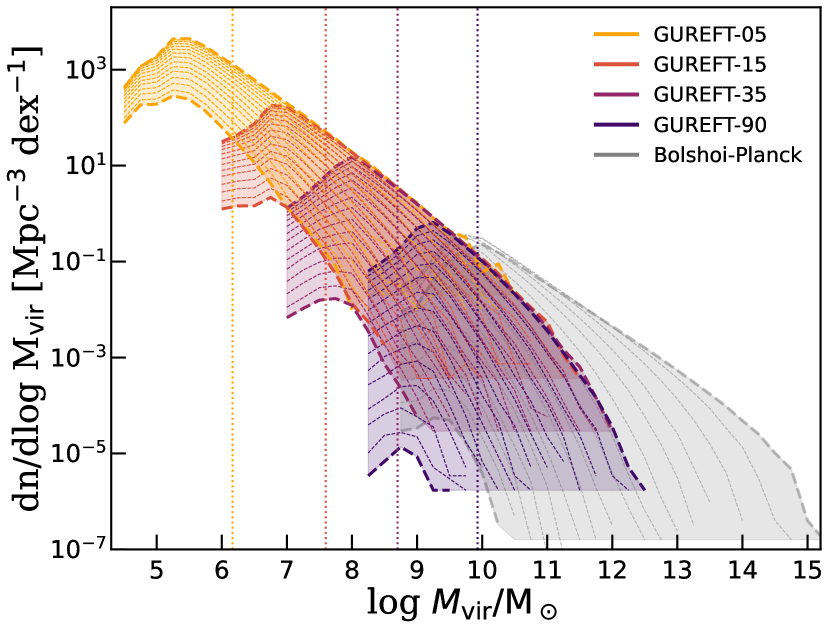
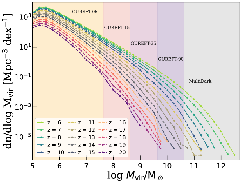
Figure 3: In this figure, we show the HMFs between $z=6$ to 20 predicted from the full suite of gureft simulations. In the left panel, we show the halo mass functions colour-coded by the gureft boxes. The shaded region shows the range between $z=6$ to 20, with individual HMFs shown by colour-matched dashed lines, with thicker lines at the boundaries ($z=6$ and 20). The vertical dotted lines mark the mass thresholds corresponding to 100 DM particles for the gureft boxes in matching colours. In addition, we show halo mass functions from the Bolshoi-Planck simulation between $z=0$ to 15 (shown in grey with matching style). In the right panel, we show the HMFs over a wide mass range obtained by combining well-resolved halo populations sourced from the four gureft boxes. In addition, the massive end of the HMFs are supplemented with the MultiDark boxes (Bolshoi-Planck for $z\lesssim 10$ and VSMDPL for $z>10$). We show shaded regions with matching colour in the right panel to indicate which simulation the halo population was drawn from. The combined gureft and Multidark simulation suites allow us to probe halo properties over an extremely broad dynamic range.

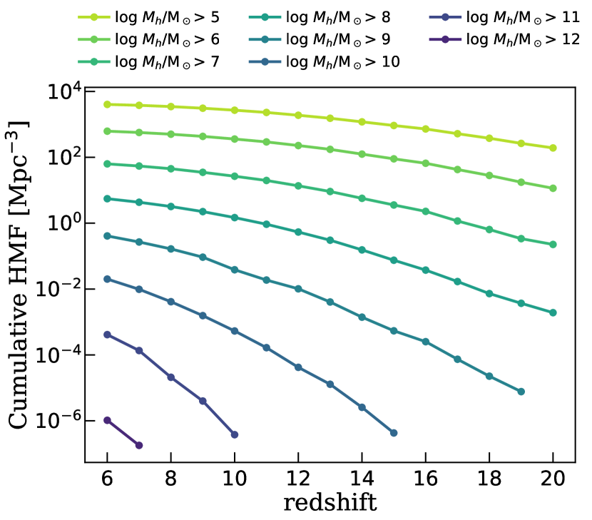
Figure 4: Cumulative number density of halos with mass above a given $M_{\text{h}}$ as a function of redshift, $n(>M_{\text{h}},z)$, calculated based on the gureft-MultiDark combined HMFs as shown in the right panel of Fig. 3. This figure provides a benchmark for the expected abundances of the dark matter halos that host galaxies and SMBH in the early Universe.

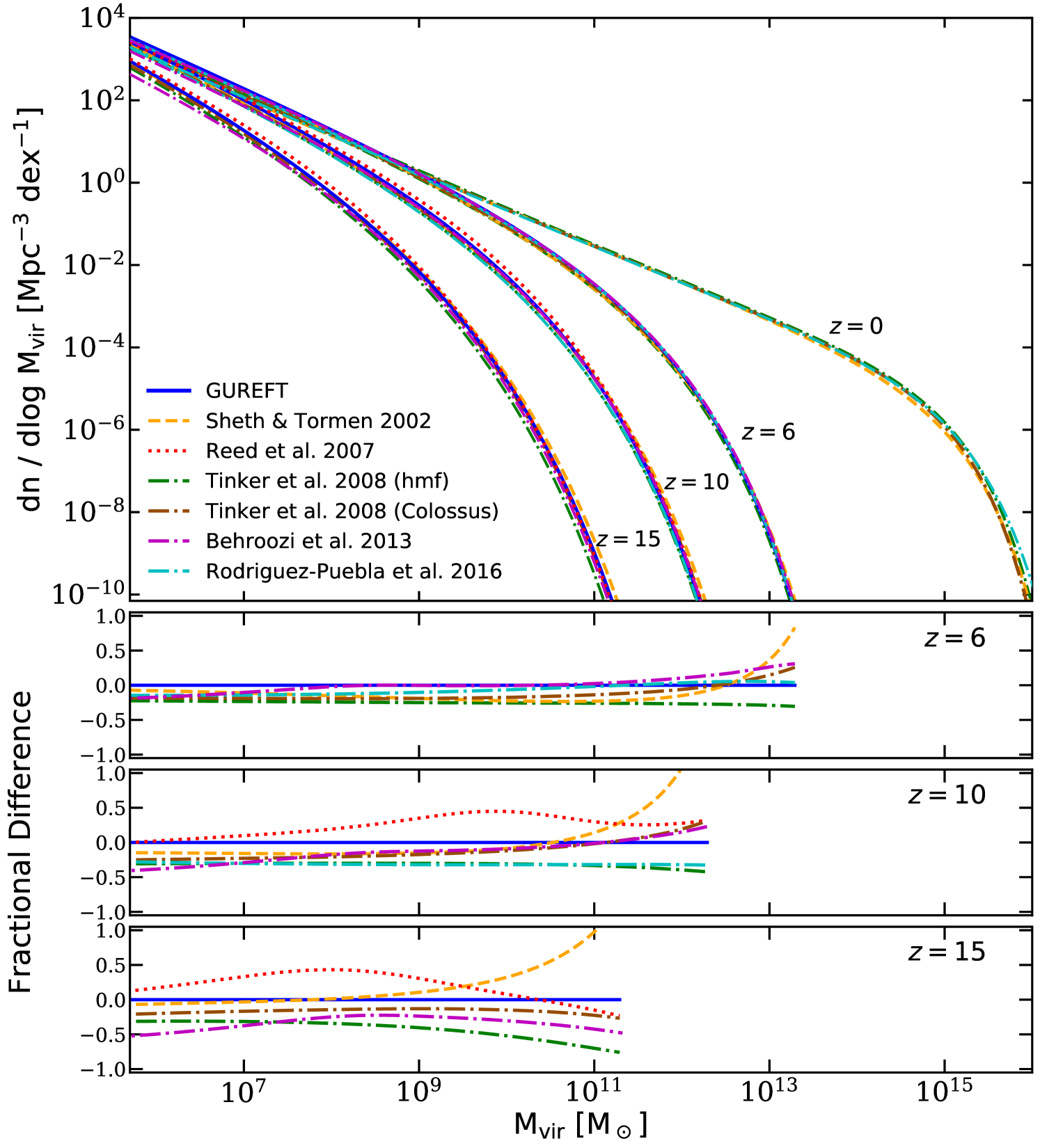
Figure 5: This figure compares the results from the gureft simulation suite (blue solid lines) at $z=6$, 10, and 15 with the HMFs commonly adopted by other high redshift-focused studies. The fits to simulations in the MultiDark suite (BolshoiP, SMDPL, and MDPL; Klypin et al., 2016), which adopted the Tinker et al. HMF parameterization and cosmological parameters matching the ones adopted by the gureft simulation suite, are shown for $z=6$ and 10 (Rodríguez-Puebla et al., 2016, cyan dot-dashed lines). The Behroozi et al. (2013c, magenta dot-dashed) HMFs also adopted the Tinker et al. parameterization, with corrections applied for 2LPT initial conditions. In additional, we also show the hmf and Colossus python packages implementations of the Tinker2008 HMFs with cosmological parameters updated to match the ones adopted in this work with the green and brown dot-dashed lines, respectively. We also show HMFs from the analytic model of Sheth & Tormen (2002, yellow dashed lines), updated to cosmological parameters and matter power spectrum reported by the Planck Collaboration (XIII 2016). Results from the high-resolution $N$-body simulations of Reed et al. (2007, red dotted), which adopted earlier WMAP cosmological parameters, are shown at $z=10$ and 15. In the top panel, we show a direct comparison of these HMFs across a wide mass range. In addition, we show a comparison among MultiDark, Tinker, and ST at $z=0$. The bottom panels show the fractional difference of the number density of halos from these HMFs relative to the gureft outputs $(\phi_{X}-\phi_{\text{{gureft}}})/\phi_{\text{{gureft}}}$ at $z=6$, 10, and 15. These commonly used analytic models and fitting functions can differ from our results by up to an order of magnitude at high redshift.

3 Results

In this section, we present results from the suite of gureft simulations. In particular, we highlight the unique results that are enabled by these new suite of simulations, and make comparisons and connections with previous work. In section 3.1–3.2, we present the halo mass functions, halo mass vs. $V_{\rm max}$ relations, concentration vs. mass relations, and the distributions of halo spin parameters at a series of output times. In 3.3, we present the halo mass assembly histories.

3.1 Halo mass functions and number densities

One-point distribution functions of halo virial mass, also known as halo mass functions (HMFs), are an important, quick diagnostic tool quantifying halo populations. In Fig. 3, we show the HMFs from the full suite of gureft simulations between $z=6$ to 20. In the left panel, we show individual HMFs from the four gureft boxes. We show the full mass range of detected halos in these boxes, including where the measurements become incomplete due to the mass resolution limit, manifested by the turnover in the HMFs. In addition, we also show HMFs from the BolshoiP simulations.

In the right panel of Fig. 3, we show HMFs that are constructed by combining results across the gureft suite. Here, halos with $\log(M_{\text{h}}/\text{M}_{\odot})\leq 7.5$ are sourced from gureft-05, $7.5<\log(M_{\text{h}}/\text{M}_{\odot})\leq 8.5$ from gureft-15, $8.5<\log(M_{\text{h}}/\text{M}_{\odot})\leq 9.5$ from gureft-35, and $\log(M_{\text{h}}/\text{M}_{\odot})>9.5$ are sourced from gureft-90. Our goal is to source halos from each box in a mass range that are both well resolved and are statistically robust, except for the low-mass end of gureft-05, for which we show the turnover to mark where the simulations are limited by resolution, and the massive end of gureft-90, where the most massive bins may contain only a handful of halos. Fig. 4 shows the cumulative number density of halos above a given mass as a function of redshift, $n(>M_{\text{h}},z)$, calculated based on the combined HMFs (see right panel in Fig. 3).

In Fig. 5, we compare the gureft HMFs at $z=6$, 10, and 15 to a number of fitting functions that are widely used in high- to ultrahigh-redshift focused studies. We show HMFs from the analytic model of Sheth & Tormen (2002), which is based on the excursion set approach (e.g. Bond et al., 1991; Sheth, 1998) that allows ellipsoidal collapse. In this comparison, we incorporated the cosmological parameters and matter power spectrum reported by the Planck Collaboration (XIII 2016), matching the ones adopted by gureft. Tinker et al. provided a HMF parameterization and HMFs that were fitted to a wide range of cosmological simulations adopting cosmological parameters reported by early phase of the WMAP mission. Rodríguez-Puebla et al. (2016) adopted the Tinker et al. parameterization to fit to simulations in the MultiDark suite (BolshoiP, SMDPL, and MDPL; Klypin et al., 2016) up to $z\sim 10$, which adopts cosmological parameters matching the ones adopted by the gureft simulation suite. The gureft results match BolshoiP by design given the matching cosmological parameters and the same halo finding methods and definitions. We note that in the Rodríguez-Puebla et al. (2016) parameterization, the parameter $b$ becomes negative and the $f(\sigma)$ function becomes undefined at $z>12.63$, and therefore is not valid for redshifts above this value.

In addition, we also show HMFs from Behroozi et al. (2013c) that adopted the same parameterization and had corrections applied for 2LPT initial conditions and the implementation of Tinker et al. (2008) HMFs from the hmf package, with cosmological parameters updated to match the ones adopted by this work using a package-provided function (shown as green dot-dashed lines). We note that the Tinker et al. HMFs shown in this comparison are specific to the implementation adopted by the hmf package. Other implementations, such as Klypin et al. (2016), have been shown to yield better agreement with $N$-body simulations that adopt Planck-compatible cosmological parameters up to $z\sim 5.5$ with updated fitting parameters for $f(\sigma)$.

Results from the high-resolution $N$-body simulations of Reed et al. (2007), which were carried out over $z\sim 30$ to 10 with earlier WMAP3 cosmological parameters are shown at $z=10$ and 15 for comparison.

The comparison in Fig. 5 shows that all modelled and fitted HMFs are in superb agreement with each other at $z=0$ and are in fairly good agreement with gureft and each other at $z\sim 6$ (e.g. within $\pm 50\%$ from gureft). However, these HMFs can evolve very differently towards the higher redshifts as they are extrapolated to regimes that were previously unconstrained. Thus, the discrepancy among them continues to widen towards ultra-high redshifts, and the differences can be up to a factor of two in both directions relative to the gureft results. We also add that despite the updated cosmological parameters in the Tinker et al. (2008) lines in the hmf and Colossus implementations, the fitting function $f(\sigma)$ is not universal to changes in cosmology and would need to be refitted (e.g. Behroozi et al., 2013c; Rodríguez-Puebla et al., 2016, and this work).

We further note that a number of recent studies that attempt to interpret observed galaxy populations at ultra-high redshift (e.g. Boylan-Kolchin, 2023; Mason et al., 2023; Ferrara et al., 2023; Dekel et al., 2023; Harikane et al., 2023a; Muñoz et al., 2023; Padmanabhan & Loeb, 2023) adopt these fits in their work. Furthermore, these results have important implications for the use of abundance matching approaches to link observed galaxy populations to dark matter halos. A fitting function and best-fit parameters for the gureft HMFs are provided in Appendix A.

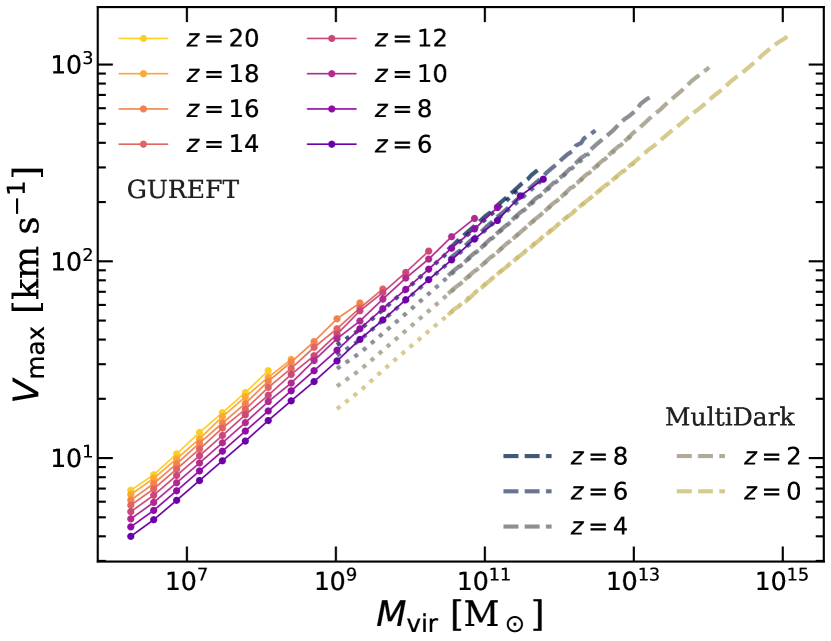
Figure 6: The median of maximum halo circular velocity, $V_{\text{max}}$, as a function of $M_{\text{vir}}$ for halos in the gureft simulation suite between $z=6$ to 20 (dotted lines). These results are compared to the SMDPL (dashed lines) and VSMDPL (dotted lines, RP16) simulations from the MultiDark suite between $z=0$ to 6. gureft shows a continuation of the trend of increasing $V_{\text{max}}$ at fixed halo mass towards earlier cosmic times that was seen at lower redshift in previous simulations.

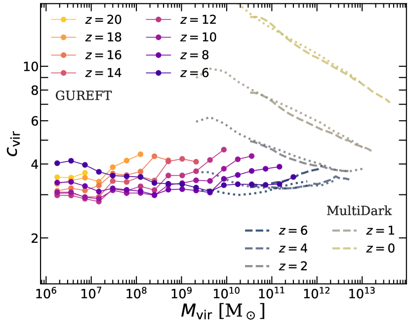
Figure 7: The median of halo concentration as a function of $M_{\text{vir}}$ between $z=6$ to 20 from the gureft suite, compared to results from the SMDPL (dashed lines, RP16) and VSMDPL (dotted lines) simulations from the MultiDark suite between $z=0$ to 6. Previous simulations showed that the concentration-mass relation decreased in normalization and flattened with increasing redshift to $z\sim 6$. gureft reveals a reversal in this trend at $z\gtrsim 6$, with the concentration at fixed mass increasing slightly towards earlier times.

3.2 Structural properties of ultra-high-redshift halos

In this subsection, we show the evolution of scaling relations among key structural properties of halos across high- to ultra-high redshifts. Similar to that of RP16 or other studies, we adopt a 100-particle threshold for halos in the gureft simulation suite to be considered well-resolved.

$V_{\text{max}}$ is an important quantity that is often utilised in sub-halo abundance matching (SHAM) and (semi-)empirical techniques (Behroozi et al., 2019; Behroozi et al., 2020; Zhang et al., 2023), and is also used by some semi-analytic models. It is defined as the rotation velocity of the halo at the maximum value of the rotation curve. In Fig. 6, we show $V_{\text{max}}$ as a function of $M_{\text{vir}}$ between $z=6$ and 20. The gureft results are combined in a similar manner to the approach used to construct the composite HMFs as demonstrated in the right panel of Fig. 3. These results are compared to the ones from the SMDPL simulation between $z=0$ to 8 as shown in RP16 and from the VSMDPL simulation accessed through the MultiDark Database (Riebe et al., 2013). We show that gureft and MultiDark are in superb agreement in mass ranges and redshifts where the two overlap.

We follow the same fitting functions as presented in RP16, where $E(z)$ is the expansion rate for a flat universe:

$$E(z)=H/H_{0}=\sqrt{\Omega_{\Lambda,0}+\Omega_{m,0}(1+z)^{3}}\text{.}$$ (1)

With this parameterization, the best-fit $V_{\text{max}}$–$M_{\text{vir}}$ relation based on gureft for halos between $6\lesssim z\lesssim 14$ is expressed as:

$$\begin{split}V_{\text{max}}(M_{\text{vir}},z)&=\beta(z)(M_{\text{vir,12}}\;E(z))^{\alpha(z)}\text{, with}\\ \alpha(z)&=0.339-0.053a+0.079a^{2}\\ \log\beta(z)&=2.171-0.114a-0.085a^{2}\text{,}\end{split}$$ (2)

where $M_{\text{vir,12}}\equiv M_{\text{vir}}/10^{12}$. We note that the fitting function presented in RP16 and other works are for mass units of M${}_{\odot}h^{-1}$. The fitting parameters in equation 2 assumes $M_{\text{vir}}$ in physical units M_⊙, the same as those plotted in Fig. 6.

Concentration and spin are two key physical properties for characterising the internal structure of dark matter halos (e.g. Bullock et al., 2001a, b). Fig. 7 shows concentration assuming a Navarro, Frenk & White (NFW; 1997) halo profile, defined as $c_{\text{vir}}\equiv R_{\text{vir}}/R_{s}$, where $R_{\text{vir}}$ is the virial radius and $R_{\text{s}}$ is the scale radius. Given the large scatter in this relation and limited dynamic range covered by these boxes, combining results from halos across multiple boxes can be tricky. For instance, the low-mass end of the ‘effective mass range’ covered by these boxes is limited by the number of particles required to resolve a halo and reliably measure its properties. On the other hand, the massive end is limited by the number of halos available in these boxes. While well-resolved halos identified with tens of thousands of particles can have properties measured more robustly, these halos are also very rare and become insufficient for robust statistical studies. We conducted a controlled experiment with the simulated $M_{\text{vir}}$–$c_{\text{vir}}$ from the gureft boxes to inform the set of criteria for combining these boxes and present the detailed findings in Appendix B.

In order to utilise predictions based on the full suite of gureft simulations, we combined together the scaling relations predicted by these boxes following the following criteria:

1. Only well-resolved halos identified with at least 100 DM particles are considered;

2. When computing scaling relations, only mass bins containing over 100 halos are included

3. In the mass range where two boxes overlap, the larger box containing more halos is preferred over the smaller box with fewer halos.

Appendix B shows that the concentration-mass relation measured in the overlapping regions of different boxes agree well when these criteria are applied.

We also note that in the halo profile fitting carried out by rockstar, $R_{\text{s}}$ is capped at $R_{\text{vir}}$. Halos with profiles that are not well-fit by an NFW profile (e.g. recent mergers, or halos with multiple density peaks) can yield unphysical measurements of $R_{\text{s}}\approx R_{\text{vir}}$. We remove these halos from the sample by requiring $(R_{\text{vir}}-R_{\text{s}})/R_{\text{vir}}>0.1$. Given that there are only very few halos with naturally occurring $c_{\text{vir}}<1.1$, this cutoff removes mostly these halos with spuriously low concentration estimates.

Fig. 7 shows the $M_{\text{vir}}$–$c_{\text{vir}}$ between $z=6$ to 20 measured from halos across the gureft boxes. This is compared with halos from the SMDPL simulations as shown by RP16 and calculated from VSMDPL. Once again, we find that gureft and MultiDark are in superb agreement where they overlap. The gureft predictions also agree with the evolution described in Diemer & Kravtsov (2015). These previous studies showed that the $M_{\text{vir}}$–$c_{\text{vir}}$ relation flattens back to $z\sim 4$, and halo concentration decreases back in time at fixed halo mass back to $z\sim 4$. There was already a hint of a reversal in this evolution from $z\sim 4$ to 6, with halos at $z\sim 6$ having slightly higher concentrations than halos of the same mass at $z\sim 4$, but the effect was subtle. Our results more definitively show that halo concentrations at fixed mass continue to increase towards earlier cosmic times back to $z\sim 20$. We discuss the physical interpretation of this behaviour in Section 4.

In Fig. 8, we show the distribution of $c_{\text{vir}}$ for halos in the mass ranges where two adjacent gureft boxes overlap, including $10<\log M_{\text{h}}/\text{M}_{\odot}<10.5$ for gureft-35 and gureft-90 at $z=6$, $9<\log M_{\text{h}}/\text{M}_{\odot}<9.5$ for gureft-15 and gureft-35 at $z=8$, and $7.7<\log M_{\text{h}}/\text{M}_{\odot}<8.2$ for gureft-05 and gureft-15 at $z=10$. This demonstrates how the distribution of $c_{\text{vir}}$ can be affected by the mass resolution and the number of halos, which is limited by the simulated volume. Fig. 8 also presents a resolution study, where we can compare the halo populations in similar mass ranges across pairs of boxes with different mass resolutions. We find that the median value of concentration is quite insensitive to resolution. However, the high concentration end of the distribution is noticeably impacted by resolution, with simulations with higher mass resolution (smaller volume) producing a narrower concentration distribution with a less pronounced tail towards high concentrations.

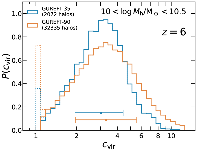
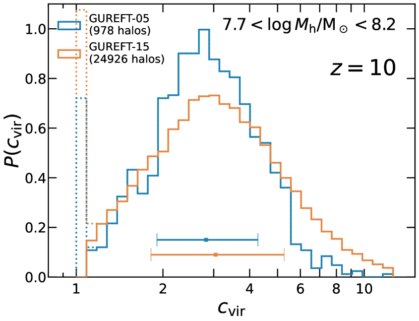
Figure 8: This figure shows the distribution of $c_{\text{vir}}$ for halos in the mass ranges where two adjacent gureft boxes, including $10<\log M_{\text{h}}/\text{M}_{\odot}<10.5$ for gureft-35 and gureft-90 at $z=6$, $9<\log M_{\text{h}}/\text{M}_{\odot}<9.5$ for gureft-15 and gureft-35 at $z=8$, and $7.7<\log M_{\text{h}}/\text{M}_{\odot}<8.2$ for gureft-05 and gureft-15 at $z=10$. The larger/lower resolution (smaller/higher resolution) box in the pair is shown in orange (blue). The $c_{\text{vir}}$ bins that satisfy the selection criteria $(R_{\text{vir}}-R_{\text{s}})/R_{\text{vir}}<0.1$ detailed in the text are shown with dotted lines, and are excluded from the rest of our analysis. The number of halos available for comparison is indicated in the upper-left corner of each plot. The data points and error bars in matching colour mark the median and 16th and 84th percentiles of the distributions. We find that the mass resolution of a cosmological simulation can have a mild impact on the resultant distribution of $c_{\text{vir}}$, where higher mass resolution yields lower concentration. This mostly affects halos in the high concentration tail, and does not have a large effect on the median concentration.

The angular momentum profile of halos is characterised by the dimensionless spin parameter, originally defined by Peebles (1969) as

$$\lambda_{\text{P}}\equiv\frac{J|E|^{1/2}}{GM^{5/2}}\text{,}$$ (3)

where $J$, $E$, and $M$ are the total angular momentum, energy, and mass of the system, respectively; and $G$ is the universal gravitational constant. Bullock et al. (2001b) presented an alternative definition, which is also widely adopted:

$$\lambda_{B}\equiv\frac{J}{\sqrt{2}MVR}\text{,}$$ (4)

where $J$ is the angular momentum inside a sphere of radius $R$ containing mass $M$; and $V$ is the halo circular velocity at radius $R$.

In Fig. 9, we show the spin parameter calculated based on both definitions, Peebles ($\lambda_{\text{P}}$) and Bullock et al. ($\lambda_{\text{B}}$), as a function of $M_{\text{vir}}$, between $z=6$ to 20. The overall higher values of $\lambda_{\text{B}}$ compared with $\lambda_{\text{P}}$ is consistent with findings from the MultiDark simulations presented by RP16. We also show results at $z=0$ to 8 based on halos from the SMDPL simulations as shown by RP16 and from VSMDPL. We add that the noisy behavior on the massive end of the SMDPL results is likely due to small samples of halos in this mass range. We note that the scale we use to plot $\lambda$ has a much smaller range than the one used in RP16, which accounts for the apparently stronger mass dependence of $\lambda$. However our results are, again, fully consistent with those of RP16 where they overlap in mass and redshift.

Similar to that for $c_{\text{vir}}$ above, we present a resolution study for $\lambda_{\text{B}}$ in Fig. 10. We find that the mass resolution of the simulation has less impact on the distribution of $\lambda_{\text{B}}$ than was the case for $c_{\text{vir}}$, with the overall distribution showing only a weak dependence on the mass resolution.

In Fig. 11, we show the evolution across redshift of the spin parameter distributions obtained by combining the four gureft boxes, as before, calculated based on both the Peebles and Bullock et al. definitions. For both definitions, we see moderate evolution in this distribution, with a shift towards lower median values of the spin parameter at earlier cosmic times. This is a continuation of the trend in $\lambda$ with redshift seen in RP16 and Somerville et al. (2018). We note that neither a log-normal distribution (see Bullock et al., 2001b) nor a double-Schechter function fit (see RP16) provides an accurate fit to the distribution of $\lambda$ at $z>6$. A new fitting function and best-fit parameters are provided in Appendix C.

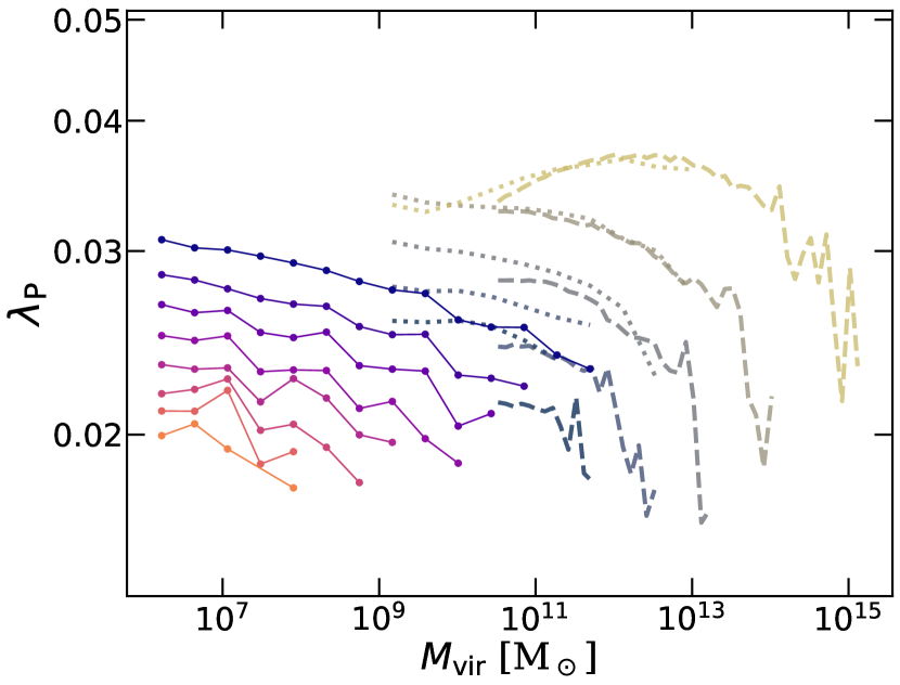
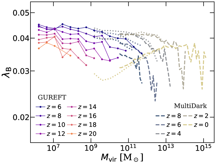
Figure 9: The median of spin parameter $\lambda$ calculated based on the definitions from (Peebles, 1969, top panel) and (Bullock et al., 2001b, bottom panel) as a function of $M_{\text{vir}}$ for halos in the gureft simulation suite. These results are compared to the ones from the SMDPL (dashed lines, RP16) and VSMDPL (dotted lines) simulations from the MultiDark suite between $z=0$ to 8. gureft shows a continuation of the trend of decreasing spin across all halo masses towards earlier cosmic times that was seen at lower redshift in previous simulations.

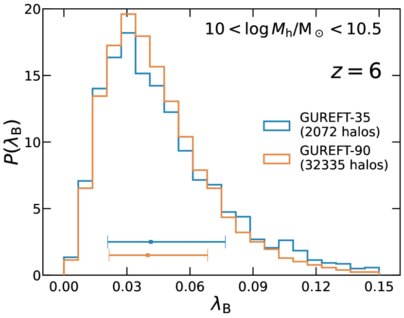
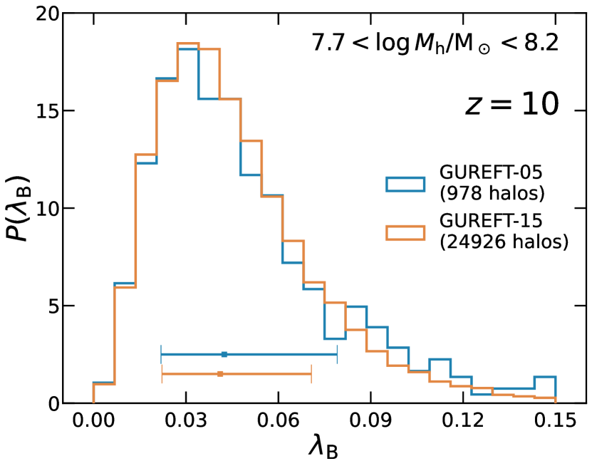
Figure 10: This figure shows the distribution of $\lambda_{\text{B}}$ for halos in the mass ranges where two adjacent gureft boxes, including $10<\log M_{\text{h}}/\text{M}_{\odot}<10.5$ for gureft-35 and gureft-90 at $z=6$, $9<\log M_{\text{h}}/\text{M}_{\odot}<9.5$ for gureft-15 and gureft-35 at $z=8$, and $7.7<\log M_{\text{h}}/\text{M}_{\odot}<8.2$ for gureft-05 and gureft-15 at $z=10$. The larger/lower resolution (smaller/higher resolution) box in the pair is shown in orange (blue). The number of halos available for comparison is indicated in the upper-left corner of each plot. The data points and error bars in matching colour mark the median and 16th and 84th percentiles of the distributions. We find that the mass resolution of a cosmological simulation can have a mild impact on the resultant distribution of $\lambda_{\text{B}}$, where higher mass resolution yields larger $\lambda_{\text{B}}$. This mostly affects halos in the high-$\lambda$ tail of the distribution, and does not have a large impact on the median spin.

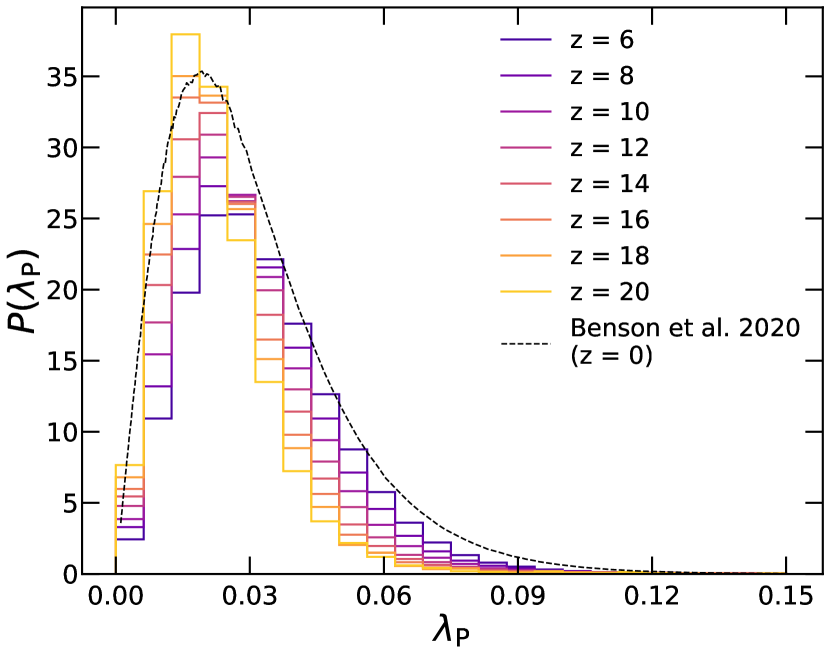
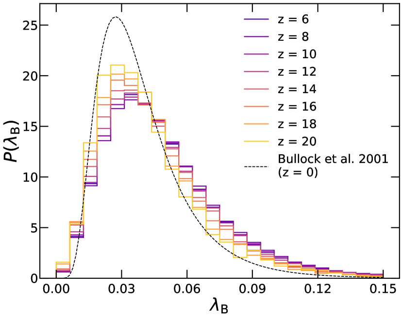
Figure 11: Normalised distributions of the spin parameter $\lambda$, calculated based on the Peebles (1969) definition (left panel) and the Bullock et al. (2001b) definition (right panel), between $z=6$ to 20. The best-fit log-normal distribution fitted to $z\sim 0$ halos for Benson et al. (2020, $\lambda_{\text{P}}$) and Bullock et al. (2001b, $\lambda_{\text{B}}$) is also shown. gureft reveals a mild evolution in $\lambda_{\text{B}}$, especially at $z\lesssim 16$, and a stronger evolution in $\lambda_{\text{P}}$ across the full redshift range explored in this work.

3.3 Halo growth, merger, and assembly histories

In this section, we investigate the predicted growth rates for halos at high- to ultra-high redshifts from the gureft simulations. The growth of dark matter halos from the suite of gureft simulations is further investigated in a companion work (Nguyen et al., 2023).

Fig. 12 shows the specific halo mass accretion rate averaged over a dynamical time as a function of $M_{\text{vir}}$. These results combine halos from across the gureft boxes following the same procedures for producing the $M_{\text{vir}}$–$V_{\text{max}}$ relation presented in Fig. 6. To put these high-redshift results in the context of the evolution across cosmic time, we also show the evolution between $z=0$ to 8 from SMDPL (RP16) and VSMDPL. We also show the analytic fitting function from Dekel et al. (2013) for comparison, and find that the analytic function that reproduces the lower redshift results from the MultiDark simulations gradually starts to deviate from the simulation results towards higher redshift and lower halo masses. We find that the slope of the $M_{\text{vir}}$–$dM_{\text{vir}}/dt$ relation from Dekel et al. (2013) is slightly steeper than the results from the gureft simulations. We also show the fitting function from Rodríguez-Puebla et al. (2016) that was fitted to the MultiDark simulations from $z=0$ to 8. Based on the same parameterization and best-fit parameters, we also show extrapolations up to $z=14$. The comparison of these fitting functions show that while they may agree well at low redshift, they can behave very differently when extrapolated to ultra-high redshift. We provide an updated fitting function below.

With a parameterization similar to that of the $V_{\text{max}}$–$M_{\text{vir}}$ relation presented in Equation 2, the best-fit equation for the $dM_{\text{vir}}/dt$–$M_{\text{vir}}$ relation for halos between $6\lesssim z\lesssim 14$ is

$$\begin{split}dM_{\text{vir}}/dt(M_{\text{vir}},z)&=\beta(z)(M_{\text{vir,12}}\;E(z))^{\alpha(z)}\text{, with}\\ \alpha(z)&=0.858+1.554a-1.176a^{2}\\ \log\beta(z)&=2.578-0.989a-1.545a^{2}\text{,}\end{split}$$ (5)

where $M_{\text{vir,12}}\equiv M_{\text{vir}}/(10^{12}$  M_⊙). Once again the fitting function assumes $M_{\text{vir}}$ is in physical units, M_⊙, instead of conventional simulation mass units, M${}_{\odot}h^{-1}$. The fitting function is based only on the four gureft boxes and should only be used in the corresponding halo mass range.

Fig. 13 shows the median of the halo mass growth history for halos arriving at a final $M_{\text{vir}}$ at $z=6$. This is calculated by tracking the largest progenitor halo back in time using the consistent trees merger trees. For comparison, we show the analytic model from Dekel et al. (2013), where the growth of halo mass is given by $M=M_{0}\;e^{-\alpha(z-z_{0})}$, where $\alpha=(3/2)s\;t_{1}\simeq 0.79$, $s=0.030$ Gyr^-1 is the inverse of the accretion time-scale and $t_{1}$ is the Hubble time. Similar to the previous figure, we find that halos at $z\gtrsim 6$ in gureft have higher growth rates than the Dekel et al. fitting functions imply. We attempted to fit the halo growth histories from gureft with the same functional as Dekel et al. (2013) and found that our results can’t be well fit by simple exponential growth.

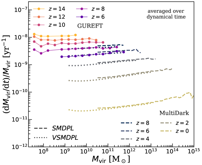
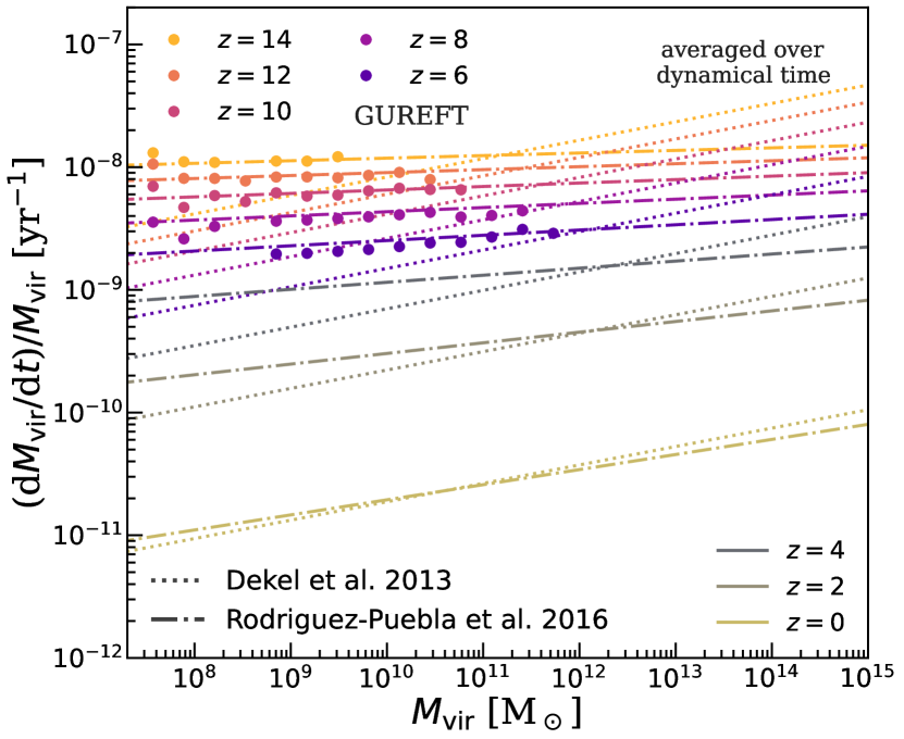
Figure 12: The left panel shows halo mass accretion rate normalised to halo mass, ($dM_{\text{vir}}/dt$)/$M_{\text{vir}}$, averaged over a dynamical time, as a function of $M_{\text{vir}}$ between $z=6$ and $14$, compared to results from the SMDPL (dashed lines, RP16) and VSMDPL (dotted lines) simulations from the MultiDark suite between $z=0$ to 8. In the right panel, we show the analytic fitting function from Dekel et al. (2013) and Rodríguez-Puebla et al. (2016) computed for $z=0$, 2, 4, 6, 8, 10, 12, and 14, shown by lines in colours matching those of the $N$-body simulations (MultiDark for $z<5$ and gureftfor $z>5$). gureft reveals a continuation of the trend of increasing $dM_{\text{vir}}/dt$ at fixed halo mass towards earlier cosmic times that was seen at lower redshift in previous simulations. The comparison with fitting functions from the literature shows that fitting functions based on lower redshifts and larger halo masses are not necessarily accurate in this regime.

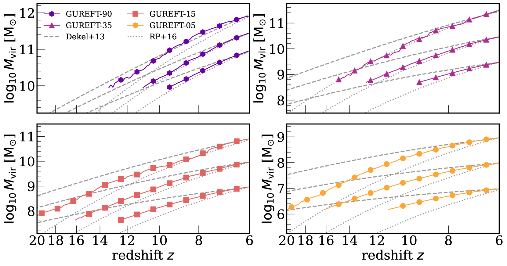
Figure 13: The median of the largest progenitor halo mass traced back in time for halos arriving at a final $M_{\text{vir}}$ at $z=6$ for halos from the gureft simulations. These results are compared to the fitting function presented by Dekel et al. (2013, grey dashed lines) and Rodríguez-Puebla et al. (2016, grey dotted lines). gureft reveals the mass accretion histories of halos in mass and redshift ranges that are first probed by our simulations. Once again, fitting functions from the literature do not necessarily perform well when extrapolated to mass and redshift ranges beyond those on which they were calibrated. The extrapolation of the Dekel et al. (2013) fitting function in general predicts earlier halo formation than our results indicate, while the Rodríguez-Puebla et al. (2016) fits perform fairly well for the higher mass halos in our GUREFT-35 and GUREFT-90 boxes, but predict later formation of the lower mass halos in GUREFT-15 and GUREFT-5.

4 Discussion

In this section, we discuss the results from the new suite of gureft simulations and the wide range of astrophysical modelling that they enable. We also discuss the implications of these new results in the context of the new era of ultra-high redshift exploration with JWST and the upcoming Roman Space Telescope. We also discuss the caveats and uncertainties in the results presented in this work.

4.1 Implications for the interpretation of high redshift populations

In the new era of ultra-high-redshift exploration enabled by JWST (Gardner et al., 2006, 2023), it is necessary to lay the ground work to support modelling and interpreting galaxies and their embedded supermassive black holes in the ultra high-$z$ universe. Shortly after the first images from JWST were released, Labbé et al. (2023) presented an analysis that claimed the discovery of several galaxies at $z\sim 8$–10 with stellar mass estimates of $\gtrsim 10^{10}M_{\rm\odot}$, with a few galaxies having estimated stellar masses of $\sim 10^{11}M_{\rm\odot}$. The question that immediately arose was whether the existence of such massive galaxies so early in the Universe would violate fundamental constraints from $\Lambda$CDM. For example, Boylan-Kolchin (2023) claimed that these galaxies were several orders of magnitude more abundant than would be expected within a standard $\Lambda$CDM paradigm. Based on an Extreme Value Statistics analysis, Lovell et al. (2022) found that these objects were in tension with $\Lambda$CDM at the $3\sigma$ level. However, Boylan-Kolchin (2023) used the predictions of the Sheth & Tormen (1999) model, which are similar to the Sheth & Tormen (2002) model. Lovell et al. (2022) use an extrapolated version of the Tinker et al. (2008) halo mass function fits, which were calibrated at much lower redshifts. As shown in Fig. 5, these analytic models and extrapolated fits can differ from our measured halo mass functions by up to an order of magnitude. Although the stellar mass estimates of the objects analyzed by Labbé et al. (2023) have now been significantly revised downwards, such that there is no longer any tension with $\Lambda$CDM (in fact many of these objects are now thought to be obscured AGN; see Barro et al. 2023), the point remains that accurate HMF estimates should be used for interpreting future observations. The fits that we provide in this work are intended to facilitate this. Moreover, the ultra high-$z$ matter assembly history captured by the suite of gureft simulations provide results critical to the development of physical models that can explain the physics that drives the early formation of these galaxies and black holes (e.g. Yung et al., 2023a).

A new generation of exascale cosmological simulations containing trillions of particles enabled by the fast-growing high performance computing capabilities, such as the new suite of Uchuu simulations (Ishiyama et al., 2021), has the capability of simulating multi-hundred-Mpc cosmological volumes with unprecedented mass resolution. However, it can cost upwards of tens of millions of CPU-hours and generate multiple petabytes of data, which will cost a significant additional amount of computing resources to analyse. In addition, many existing halo finders and merger tree construction codes are not optimised to handle data of such volume. Therefore, solving this problem by brute force is not practical. The tiered box approach explored in this work provides a computationally efficient and elegant alternative.

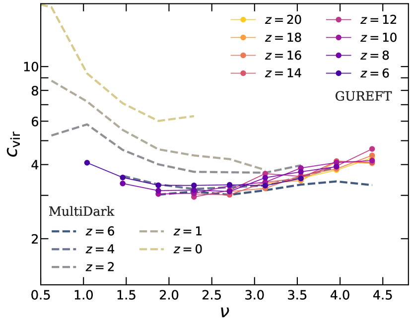
Figure 14: The median of halo concentration as a function of peak height $\nu$, between $z=6$ to 20 for halos in the gureft simulation suite. We also computed this relation for halos in the VSMDPL simulations (dashed lines) from the MultiDark suite between $z=0$ to 6 for comparison. This illustrates that halo concentration is self-similar and remains invariant at ultra-high $z$ and across a wide redshift range.

4.2 Interpretation of the trends in halo properties

Given the limitations in mass resolution and stored snapshots from past cosmological simulations, the key structural properties and assembly histories of these halos, are often inferred by extrapolating fitting functions that were previously fitted to low redshift to untested territories, both into the earlier universe and mass range below the resolution limits of these simulations. In this work, we directly simulate these halos and provide a first look into the distribution of ultra-high $z$ redshift halos by mass, as well as their key structural properties and mass assembly histories. We have shown that these commonly used extrapolations often do not accurately represent the ultra-high redshift halo populations.

The suite of gureft simulations, for the first time, demonstrates the evolution of various halo properties out to ultra-high redshifts and demonstrated that some relations seem to continue the trends seen at lower redshift (e.g. $M_{\text{vir}}$–$V_{\text{max}}$, $M_{\text{vir}}$–$dM_{\text{vir}}/dt$, and $M_{\text{vir}}$–$dM_{\text{vir}}/dt$). However, gureft results also reveal a reversal in the $M_{\text{vir}}$–$c_{\text{vir}}$ relation at $z\gtrsim 6$, where the median concentration for intermediate-mass halos (e.g. $9\lesssim\log(M_{\text{h}}/\text{\;M${}_{\odot}$})\lesssim 12$) seems to increase between $6\lesssim z\lesssim 14$.

Numerous past studies have explored the origin of halo density profiles and halo concentration-mass relations (e.g. Navarro et al., 1996; Bullock et al., 2001a), finding strong ties between these properties and halo mass accretion history (Wechsler et al., 2002; Zhao et al., 2003). Halo mass accretion history in turn is known to be highly correlated with the height of the density peak within which the halo forms. Assuming that matter is distributed following a linear Gaussian overdensity field, the peak height quantifies how statistically rare a halo of a given mass at a given cosmic epoch is, and is defined as $\nu\equiv\delta_{\text{c}}/\sigma(M_{\text{h}},z)$, where $\delta_{\text{c}}$ is the critical over-density required for spherical collapse at $z$ and $\sigma(M_{\text{h}},z)$ is the root-mean-square fluctuation of the smoothed density field. Several numerical studies have shown that expressing halo mass in terms of peak height removes much of the evolution of concentration as a function of redshift (e.g. Dalal et al., 2008; Zhao et al., 2009; Prada et al., 2012; Ludlow et al., 2014; Dutton & Macciò, 2014). Building on this work, Diemer & Kravtsov (2015) presented a model in which halo concentration is a function of peak height and the local slope of the power spectrum, where the latter is needed to explain the redshift evolution in the $c$–$\nu$ relation seen between $z\sim 0$ to 6.

To further investigate the underlying drivers for the redshift evolution in halo structural properties presented in Section 3.2, we show in Fig. 14 halo concentration as a function of peak height corresponding to a given halo mass. In our analysis, this quantity is computed using the peakHeight function from the Colossus python package (Diemer, 2018). This calculation adopts a value for uniform-density spherical collapse, $\delta_{\text{c}}\approx 1.686$, derived from the spherical top-hat collapse model in an Einstein-de Sitter universe (Gunn & Gott, 1972). We note that the median $c_{\text{vir}}$–$\nu$ relation presented in Fig. 14 is binned separately after peak height is computed for individual halos, rather than translating the binned $c_{\text{vir}}$–$M_{\text{vir}}$ relation. We also calculate this quantity for halos in VSMDPL for comparison.

As demonstrated in Fig. 14, the $c_{\text{vir}}$–$\nu$ relation exhibits negligible evolution over the redshift range $6\lesssim z\lesssim 20$. This result is highly consistent with the prediction of the Diemer & Kravtsov (2015) model, as the other main dependency in their universal model, the local slope of the power spectrum, defined as $n(k)\equiv d\ln P(k)/d\ln k$, evolves very little across this redshift range (i.e., the power spectrum is close to self-similar in this regime).

4.3 Caveats and limitations

As part of this work, we conducted a few controlled experiments to better characterise the effective mass range covered by individual simulations and explored the impact on the predicted halo populations due to the volumes and resolution of the simulations. In addition to the previously mentioned dynamic range limitations due to simulated volume and resolution, we also find that the mass resolution may have an impact on the predicted physical properties of halos. We make use of the overlapping mass range between adjacent gureft boxes to study the potential impact on the simulated halo populations due to differences in mass resolution. The simulated results overall converge extremely well across boxes, including halo number density (see Fig. 3 for HMF) and the median of scaling relations (see Fig. 16 for $M_{\text{vir}}$–$c_{\text{vir}}$ relation).

As shown in Figs. 8 and 10, we show the normalised distribution functions for $c_{\text{vir}}$ and $\lambda_{\text{B}}$ for halos in overlapping mass range between two adjacent gureft boxes. We find that halos in the lower resolution box (plotted in orange) tend to have slightly overall higher $c_{\text{vir}}$ and lower $\lambda_{\text{B}}$ than halos in the simulated volume with higher mass resolution. Halos in simulations with lower mass resolution tend to have their scale radius under-estimated. While the difference in the resultant distribution is rather subtle, we need to exercise some caution when combining result across different boxes. We also note that in the context of gureft (or other cosmological simulations when considering the trade off between simulated volume and mass resolution), while halos are better-resolved and better-characterised with a higher number of particles in boxes with higher mass resolutions, for a fixed number of particles the number of halos available in the higher-resolution (hence smaller) boxes would be significantly fewer than in the larger box, which could lead to an incomplete sampling of the true dispersion in the distributions and scaling relations (see Fig. 16). When combining scaling relations across gureft boxes, we prioritise results from larger boxes over smaller ones in order to obtain better statistics.

We also note the mass ranges covered by the gureft suite, especially gureft-05 and gureft-15, are sensitive to the small-scale behaviour of dark matter. As shown by (Kulkarni & Ostriker, 2022), fuzzy dark matter (FDM; e.g. Khlopov et al. 1985; Hui et al. 2017) can cause deviations in the HMF at $z=0$ for halos with $M_{\text{h}}<10^{11}$  M_⊙ and a difference in halo number density up to $\sim 2$ dex for $M_{\text{h}}\sim 10^{7}$  M_⊙. Kulkarni & Ostriker also showed that it can substantially impact the low-mass end slope ($\log M_{\text{h}}/\text{M}_{\odot}\lesssim 11$) of the HMF at $z=0$. At $z\sim 4$, virtually no halos with $M_{\text{h}}<10^{8}$  M_⊙ are able to form (Schive et al., 2016). Similarly, in a warm dark matter (WDM; e.g. Dodelson & Widrow 1994) scenario, the halo number density at $M_{\text{h}}<10^{9}$  M_⊙ can significantly deviate from that in the CDM model (Gilman et al., 2020). Deep-field galaxy surveys with JWST may provide insights that can help indirectly constrain dark matter models.

5 Summary and Conclusions

This paper presents the new gureft suite of four dark matter-only, cosmological $N$-body simulations, which were carefully designed to capture the emerging halo populations and their merger histories at high to ultra-high redshifts ($6\lesssim z\lesssim 20$). The suite of gureft simulations fill in the gap where the earliest episode of halo assembly histories are not covered by existing cosmological-scale dark matter-only simulations. We provide a comprehensive overview of the predicted distribution functions for key physical properties, including virial mass $M_{\text{vir}}$, concentration $c_{\text{vir}}$, and spin $\lambda$, and scaling relations between $M_{\text{vir}}$ and maximum rotation velocity $V_{\text{max}}$, $c_{\text{vir}}$, $\lambda$, and halo growth rate $dM_{\text{vir}}/dt$. In addition, we present accurate updated fitting functions over the halo mass range and redshift range that is relevant at high redshift.

We summarise our main conclusions below.

1. By combining simulated halo populations from all four gureft volumes, we presented halo mass functions (HMF) between $z\sim 6$ to 20 for halos across a very wide mass range $\log M_{\text{h}}/\text{M}_{\odot}\sim 5$ to 12. In addition, we provide an updated fitting function that accurately describes the HMF over this mass and redshift range.

2. Fitting functions for the HMF from the literature, as well as analytic models based on the Extended Press Schechter formalism (e.g. Sheth et al., 2001) can disagree with the results from gureft by several tenths of a dex up to 1 dex at ultra-high redshifts ($z\gtrsim 10$).

3. The normalisation of the halo $M_{\text{vir}}$ vs. $V_{\text{max}}$ relation continues to increase monotonically from $z\sim 6$–20, continuing the trend previously seen from $z\sim 0$–6. We find that the relation increases by $\sim 0.25$ dex from $z\sim 0$ to 20.

4. gureft reveals a continuation of the trend seen in previous studies of decreasing spin across all halo masses towards higher redshifts. The probability distribution of $\lambda_{\text{B}}$ evolves only mildly between $6\lesssim z\lesssim 20$, whilst the distribution of $\lambda_{\text{P}}$ evolves more significantly. We provide fitting functions for these distributions.

5. We find that the $M_{\text{vir}}$–$c_{\text{vir}}$ relation, which was known to flatten at $z\sim 4$–6, remains rather flat towards higher redshifts $6$–20. In addition, the normalization of the relation increases mildly, such that halos at earlier cosmic epochs have higher concentration at fixed mass.

6. Specific halo mass accretion rates $\dot{M}/M$ at fixed halo mass continue to increase monotonically with increasing redshift from $6$–20, again continuing the trend at lower redshift, but the slope of the $\dot{M}/M$ relation flattens slightly at earlier times.

7. Fitting functions for $M_{\text{vir}}$–$dM_{\text{vir}}/dt$ and the median of the largest progenitor mass over cosmic time derived from simulations of larger mass halos at later times are not accurate when extrapolated to the smaller halo masses and higher redshifts that are probed by gureft. We provide updated fits for this regime.

8. We used halos in the overlapping mass and redshift ranges for two adjacent gureft boxes to perform a limited convergence study. We found that the differences in mass resolution has a small but systematic impact on the predicted distribution of concentration and spin, mainly affecting the highest concentration and highest spin halos. These extreme halos have lower estimated $c_{\text{vir}}$ and higher $\lambda_{\text{B}}$ in the simulations with higher mass resolution.

These new dark matter-only simulations provide a framework for modelling and interpreting the first galaxies and black holes in the early universe that can be observed with JWST.

Data Availability

The simulated data underlying this paper are stored in a private repository and will be made available upon request. The derived data products will be released through a web portal.

Appendix A Fitting parameters to high-redshift halo mass function

We provide best-fit parameters for simulated ultra- high $z$ HMFs following the same parameterization from Tinker et al. (2008) and Rodríguez-Puebla et al. (2016). The comoving number density of halos of mass between $M_{\text{vir}}$ + $dM_{\text{vir}}$ is given by

$$\frac{dn_{\text{h}}}{dM_{\text{vir}}}=f(\sigma)\frac{\bar{\rho}_{\text{m}}}{M_{\text{vir}}^{2}}\left|\frac{d\ln\sigma^{-1}}{d\ln M_{\text{vir}}}\right|\text{,}$$ (6)

where $\bar{\rho}_{\text{m}}$ is the critical matter density in the Universe, $\sigma$ is the amplitude of the perturbations, and $f(\sigma)$ is called the halo multiplicity function, which takes the form of

$$f(\sigma)=A\left[\left(\frac{\sigma}{b}\right)^{-a}+1\right]e^{-c/\sigma^{2}}\text{,}$$ (7)

where $\chi_{i}=A$, $a$, $b$, and $c$ are free parameters, given by $\chi_{i}=\chi_{0,i}+\chi_{1,i}z+\chi_{2,i}z^{2}$ with the best-fit parameters fitted to gureft+MultiDark HMFs between $z=6$ to 19. We have also updated the approximation for $\sigma(M_{\text{vir}})$ using the same functional form given by Rodríguez-Puebla et al. (2016) to fit to a wider halo mass range of $6<\log(M_{\text{vir}}/\text{M}_{\odot}h^{-1})<13$:

$$\sigma(M_{\text{vir}})=\frac{22.87988436y^{0.4069515}}{1+5.65110544y^{0.23076429}+4.02321628y^{0.36760932}}\text{,}$$ (8)

where $y\equiv 1/M_{\text{vir,12}}$ and $M_{\text{vir,12}}\equiv M_{\text{vir}}/(10^{12}$  M_⊙ $h^{-1}$). We note that the HMF fitting parameters provided by previous studies were fitted to HMFs in conventional simulation units (e.g. masses in M${}_{\odot}\,$h^-1 and distances in Mpc h^-1). However, we find it more helpful to also show fits for HMFs in physical units (e.g. masses in M_⊙ and distances in Mpc). For $\sigma(M_{\text{vir}})$ fitting function with no $h$ scaling:

$$\sigma(M_{\text{vir}})=\frac{26.80004233y^{0.40695158}}{1+6.18130098y^{0.23076433}+4.64104008y^{0.36760939}}\text{,}$$ (9)

where $y\equiv 1/M_{\text{vir,12}}$ and $M_{\text{vir,12}}\equiv M_{\text{vir}}/(10^{12}$  M_⊙). Here we present fitted parameters for both h scaled simulation units and physical units in Table 2 and Table 3, respectively.

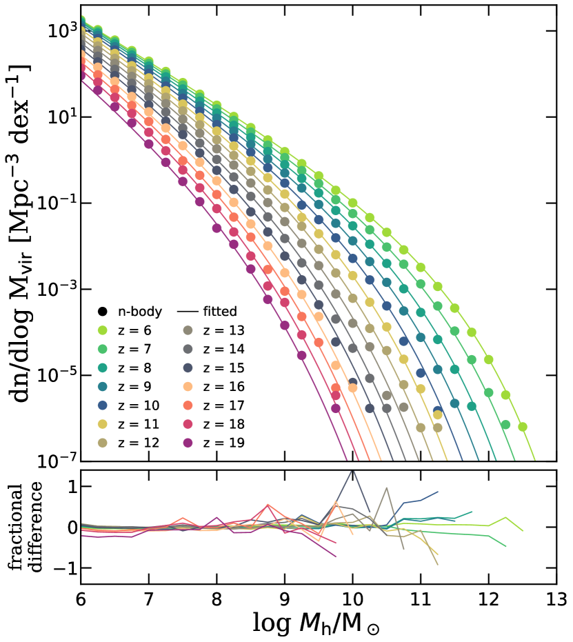
Figure 15: Top panel: Halo mass function from $n$-body simulations (data points; gureft+ MultiDark, see Fig. 3 and associated text) and fitting functions (solid lines) between $z=6$ and 19. The lines and data points are colour-coded by redshift. Bottom panel: The fractional differences between the $n$-body HMFs and fitting functions ($\phi_{\text{fitted}}-\phi_{\text{n-body}})/\phi_{\text{n-body}}$.

Table 2: Fitting parameters for the combined gureft+MultiDark HMFs fitted in conventional simulation units of [M${}_{\odot}\,h^{-1}$] and [Mpc${}^{-3}\,h^{3}\,$dex^-1].

$\chi_{i}$	$\chi_{0,i}$	$\chi_{1,i}$	$\chi_{2,i}$
A	$0.11416632$	$-0.01486746$	$0.00137191$
a	$1.05274399$	$0.02803087$	$-0.00306126$
b	$8.62813020$	$0.00384969$	$-0.02349983$
c	$1.13138924$	$0.01713172$	$-0.00113630$

Table 3: Fitting parameters for the combined gureft+MultiDark HMFs fitted in physical units of [$M_{\odot}$] and [Mpc^-3 dex^-1].

$\chi_{i}$	$\chi_{0,i}$	$\chi_{1,i}$	$\chi_{2,i}$
A	$0.13765772$	$-0.01003821$	$0.00102964$
a	$1.06641384$	$0.02475576$	$-0.00283342$
b	$4.86693806$	$0.09212356$	$-0.01426283$
c	$1.19837952$	$-0.00142967$	$-0.00033074$

Appendix B Effective mass range of gureft boxes for scaling relations

Figure 16: This set of plots show the convergence diagnostics for simulated halo populations found in the suite of gureft boxes at $z=6,7,8,10,12,15$. The top panels of these plots show histograms simply show counts of halos found in gureft (not normalised to binsize or simulated volume). These histograms include halos identified with at least 100 dark matter particles (shown in semi-transparent colours) and at least 500 particles (shown in solid colours). The horizontal grey dashed line marks where the halo count equals 100. The bottom panels show the predicted $M_{\text{vir}}$–$c_{\text{vir}}$ relations for halos from gureft, shown in matching colour as the histograms above. The median and 16th and 84th percentiles are computed in bins matching the histograms and are marked by the solid and dashed lines, respective. These lines turn semi-transparent for bins containing few than 100 halos. The underlying distribution of data points from gureft are shown in distinct shades of grey.

In this work, we presented selected scaling relations for key physical properties for halos from the suite of gureft simulations. With different simulated volume and mass resolution, these boxes are expected to cover different mass ranges, with the low-mass end limited by the mass of DM particles and the number of particles required to resolve a halo (a 100-particle threshold is adopted in this work) and the massive end limited by the simulated volume. In this appendix, we provide in-depth diagnostics of the behaviour of the halo populations in the gureft boxes and explain the decisions made in combining the scaling relations predictions as presented in 3.2.

We experiment with the threshold on DM particle number used to consider a halo resolved to assess its impact on the predicted physical quantities. In Fig. 16, we show the median scatter of the $M_{\text{vir}}$–$c_{\text{vir}}$ at various redshifts for all gureft volumes. The halos included in this plot contain $\geq 100$ dark matter particles. The histogram in the top of each panel can be used to indicate the 500-particle threshold, which occurs when the histograms transition from solid to semi-transparent. For gureft-15, -35, and -90, the mass range in between 100 and 500 particles can be cross-checked with the massive-end of gureft-05, -15, and -35, respectively, between $z=6$ to 10, where there are sufficient halos to predict the $M_{\text{vir}}$–$c_{\text{vir}}$ relation. Given that there are no significant resolution effects observed in the $M_{\text{vir}}$–$c_{\text{vir}}$ relation below the 500-particle threshold, we can safely conclude that halos with 100 particles are sufficient for rockstar to reliably measure $c_{\text{vir}}$. In an internal test, we find that the $c_{\text{vir}}$ measured by rockstar demonstrates a sharp jump for halos identified with $\lesssim 85$ particles, where these halos have systematically higher $R_{\text{s}}$. This indicates that $c_{\text{vir}}$ is cannot be accurately measured for halos made up of fewer DM particles.

In this experiment, we also find that the sample size has a significant impact on the scatter in the $M_{\text{vir}}$–$c_{\text{vir}}$ relation. It is clear that when the low-mass end of a larger box overlaps with the massive end of a smaller box, even though both halo populations are considered well-resolved, scatter in the predicted $M_{\text{vir}}$–$c_{\text{vir}}$ relation seems to be affected by the sample size available, given that the massive end of a smaller box would contain significantly fewer halos than the low-mass end of a larger box. This discrepancy systematically persists across all boxes and redshifts. We also note that this is a consequence that follows the halo populations that naturally occur in cosmological simulations, where there are fewer massive halos than low-mass halos because of hierarchical structure formation. Since we also find that the low-mass end of a larger box can more reliably predict scaling relations than the massive-end of a smaller box, we prioritise results from the smaller box over the mass range where two boxes overlap.

Appendix C Fitting the distribution of spin

The distribution of the halo spin parameter at $z\sim 0$ has been shown the be well-fitted with a modified log-normal distribution (Bullock et al., 2001b) and a Schechter-like function RP16. Here, we provide fitting functions and parameters for the high- to ultra-high-redshift spin distributions with a non-linear least-squares method. Following the approach of Bullock et al. (2001b), we fit the distribution with a log-normal distribution function

$$P(\log\lambda)=\frac{1}{\lambda\sqrt{2\pi\sigma^{2}}}\exp\left(-\frac{\log^{2}(\lambda/\lambda_{0}))}{2\sigma^{2}}\right)\text{,}$$ (10)

where $\log$ denotes natural log. We note that this is different from the (modified) log-normal distribution adopted by RP16

$$P(\log\lambda)=\frac{1}{\sqrt{2\pi\sigma^{2}}}\exp\left(-\frac{\log_{10}^{2}(\lambda/\lambda_{0}))}{2\sigma^{2}}\right)\text{,}$$ (11)

which differs by a factor of $1/\lambda$ and $\log_{10}$ is used instead of natural log. Thus, the fitting parameters provided in Table 4 are not directly comparable to the ones presented in table 7 in RP16. We also adopted a Schechter-like fit similar to the one presented by RP16

$$P(\log\lambda)=\frac{f(\lambda)}{\int_{-\infty}^{\infty}\!f(\lambda)\,\mathrm{d}\lambda}\text{,}$$ (12)

where

$$f(\lambda)=\left(\frac{\lambda}{\lambda_{0}}\right)^{\alpha}\exp\left[-\left(\frac{\lambda}{\lambda_{0}}\right)^{\beta}\right]\text{.}$$ (13)

Here, we modified the sign of the exponent from $-\alpha$ to $\alpha$. We find that integrating $f(\lambda)$ in its original form as presented in RP16 with $\alpha>0$ does not converge. We note that this modification is also needed in order to reproduce the results presented in fig. 21 in RP16. The best-fit parameters using this Schechter-like fitting function are presented in Table 5. We also note that the colour-label of fig. 21 in RP16 should be blue (black) for $\lambda_{\text{B}}$ ($\lambda_{\text{P}}$), opposite to the caption indicated.

In this Appendix, we explore fitting the distribution of $\lambda$ at higher redshifts. Similar to the findings reported by RP16, the log-normal distribution consistently under fits the distribution of low $\lambda$. On the other hand, the log-normal fit seems to reproduce the distribution of high $\lambda$ for both $\lambda_{\text{P}}$ and $\lambda_{\text{B}}$. Overall, the Schechter-like fit is able to well-represent the overall distribution of $\lambda_{\text{B}}$.

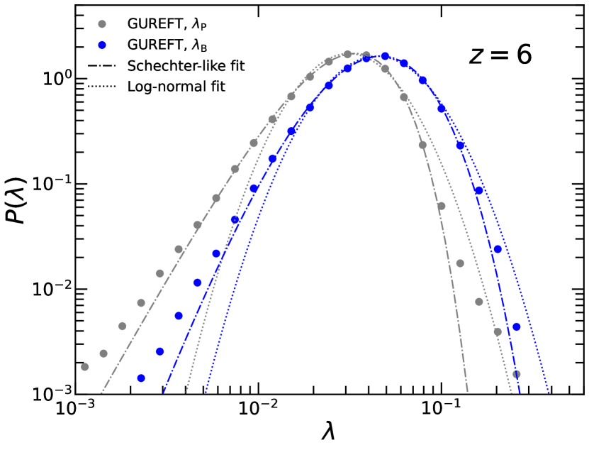
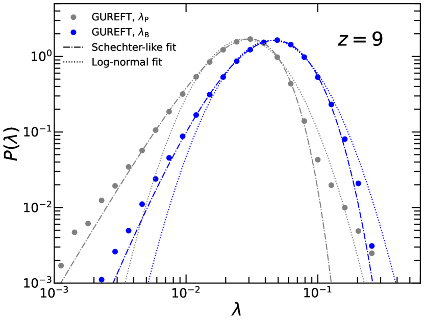
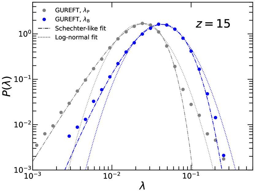
Figure 17: Halo spin distribution for halos in the gureft simulations at $z=6$, 9, 12, and 15, where $\lambda_{\text{B}}$ and $\lambda_{\text{P}}$ are denoted by blue and grey, respectively. The data points shows the probability distribution function from the simulated halos, and fitted distribution with a log-normal and Schechter-like function are shown by dotted and dot-dashed lines, respectively.

Table 4: Best-fitting parameters for the distribution of $\lambda_{\text{P}}$ and $\lambda_{\text{B}}$ using the log-normal distribution function between $z=6$ to 19.

	fitting for $P(\lambda_{\text{P}})$		fitting for $P(\lambda_{\text{B}})$
$z$	$\sigma_{\text{P}}$	$\log\lambda_{\text{0,P}}$	$\sigma_{\text{B}}$	$\log\lambda_{\text{0,B}}$
6	0.5310	-1.5067	0.5622	-1.3517
7	0.5355	-1.5231	0.5619	-1.3475
8	0.5388	-1.5395	0.5621	-1.3450
9	0.5420	-1.5552	0.5624	-1.3483
10	0.5390	-1.5677	0.5631	-1.3517
11	0.5427	-1.5808	0.5657	-1.3562
12	0.5411	-1.5944	0.5656	-1.3617
13	0.5399	-1.6063	0.5642	-1.3682
14	0.5419	-1.6221	0.5710	-1.3773
15	0.5466	-1.6345	0.5669	-1.3862
16	0.5408	-1.6462	0.5705	-1.3926
17	0.5399	-1.6582	0.5674	-1.4001
18	0.5374	-1.6634	0.5642	-1.4078

Table 5: Best-fitting parameters for the distribution of $\lambda_{\text{P}}$ and $\lambda_{\text{B}}$ using the Schechter-like distribution function between $z=6$ to 18.

	fitting for $P(\lambda_{\text{P}})$			fitting for $P(\lambda_{\text{B}})$
$z$	$\alpha_{\text{P}}$	$\beta_{\text{P}}$	$\log\lambda_{\text{0,P}}$	$\alpha_{\text{B}}$	$\beta_{\text{B}}$	$\log\lambda_{\text{0,B}}$
6	2.1144	1.2226	-1.8039	4.1486	0.6279	-2.7865
7	2.0305	1.2399	-1.8002	3.9323	0.6577	-2.6564
8	2.0705	1.2052	-1.8414	3.9215	0.6582	-2.6509
9	1.9712	1.2387	-1.8252	3.6211	0.7037	-2.4868
10	2.0256	1.2248	-1.8529	3.8948	0.6596	-2.6497
11	1.9453	1.2478	-1.8432	4.1280	0.6223	-2.8074
12	1.8490	1.3056	-1.8161	3.6061	0.6971	-2.5149
13	1.9517	1.2585	-1.8642	3.5591	0.7095	-2.4836
14	1.9173	1.2647	-1.8725	3.3529	0.7261	-2.4237
15	1.8367	1.2879	-1.8624	3.6823	0.6820	-2.5905
16	2.0303	1.2158	-1.9373	3.8166	0.6533	-2.6986
17	2.2248	1.1333	-2.0254	5.1768	0.5088	-3.5139
18	1.9551	1.2694	-1.9170	3.9704	0.6471	-2.7550

References

- Adams et al. (2022) Adams N. J., et al., 2022, MNRAS, 518, 4755
- Arrabal Haro et al. (2023) Arrabal Haro P., et al., 2023, ApJL, 951, L22
- Atek et al. (2022) Atek H., et al., 2022, MNRAS, 519, 1201
- Bagley et al. (2023) Bagley M. B., et al., 2023, arXiv:2302.05466
- Barro et al. (2023) Barro G., et al., 2023, arXiv:2305.14418
- Baugh et al. (2006) Baugh C. M., Benson A. J., Cole S., Frenk C. S., Lacey C., 2006, Mass Galaxies Low High Redshift, pp 91–96
- Behroozi et al. (2013a) Behroozi P. S., Wechsler R. H., Wu H.-Y., 2013a, ApJ, 762, 109
- Behroozi et al. (2013b) Behroozi P. S., Wechsler R. H., Wu H.-Y., Busha M. T., Klypin A. A., Primack J. R., 2013b, ApJ, 763, 18
- Behroozi et al. (2013c) Behroozi P. S., Wechsler R. H., Conroy C., 2013c, ApJ, 770, 57
- Behroozi et al. (2019) Behroozi P., Wechsler R. H., Hearin A. P., Conroy C., 2019, MNRAS, 488, 3143
- Behroozi et al. (2020) Behroozi P., et al., 2020, MNRAS, 499, 5702
- Benson (2010) Benson A. J., 2010, New Astron., 17, 175
- Benson et al. (2020) Benson A., Behrens C., Lu Y., 2020, MNRAS, 496, 3371
- Bond et al. (1991) Bond J. R., Cole S., Efstathiou G., Kaiser N., 1991, ApJ, 379, 440
- Boylan-Kolchin (2023) Boylan-Kolchin M., 2023, Nat. Astron., 7, 731
- Boylan-Kolchin et al. (2009) Boylan-Kolchin M., Springel V., White S. D. M., Jenkins A., Lemson G., 2009, MNRAS, 398, 1150
- Bryan & Norman (1998) Bryan G. L., Norman M. L., 1998, ApJ, 495, 80
- Bullock et al. (2001a) Bullock J. S., Kolatt T. S., Sigad Y., Somerville R. S., Kravtsov A. V., Klypin A. A., Primack J. R., Dekel A., 2001a, MNRAS, 321, 559
- Bullock et al. (2001b) Bullock J. S., Dekel A., Kolatt T. S., Kravtsov A. V., Klypin A. A., Porciani C., Primack J. R., 2001b, ApJ, 555, 240
- Castellano et al. (2022) Castellano M., et al., 2022, ApJL, 938, L15
- Cole et al. (2000) Cole S., Lacey C., Baugh C., Frenk C., 2000, MNRAS, 319, 168
- Conselice et al. (2003) Conselice C. J., Chapman S. C., Windhorst R. a., 2003, Astrophys. J. ApJ, 596, 2001
- Crocce et al. (2006) Crocce M., Pueblas S., Scoccimarro R., 2006, MNRAS, 373, 369
- Croton et al. (2016) Croton D. J., et al., 2016, ApJS, 222, 22
- Curtis-Lake et al. (2022) Curtis-Lake E., et al., 2022, arXiv:2212.04568
- Dalal et al. (2008) Dalal N., White M., Bond J. R., Shirokov A., 2008, ApJ, 687, 12
- Dayal et al. (2014) Dayal P., Ferrara A., Dunlop J. S., Pacucci F., 2014, MNRAS, 445, 2545
- Dayal et al. (2019) Dayal P., Rossi E. M., Shiralilou B., Piana O., Choudhury T. R., Volonteri M., 2019, MNRAS, 486, 2336
- DeRose et al. (2019) DeRose J., et al., 2019, ApJ, 875, 69
- Dekel et al. (2013) Dekel A., Zolotov A., Tweed D., Cacciato M., Ceverino D., Primack J. R., 2013, MNRAS, 435, 999
- Dekel et al. (2023) Dekel A., Sarkar K. C., Birnboim Y., Mandelker N., Li Z., 2023, MNRAS, 523, 3201
- Diemer (2018) Diemer B., 2018, ApJS, 239, 35
- Diemer & Kravtsov (2015) Diemer B., Kravtsov A. V., 2015, ApJ, 799, 108
- Dodelson & Widrow (1994) Dodelson S., Widrow L. M., 1994, Phys. Rev. Lett., 72, 17
- Donnan et al. (2022) Donnan C. T., et al., 2022, MNRAS, 518, 6011
- Drakos et al. (2022) Drakos N. E., et al., 2022, ApJ, 926, 194
- Dutton & Macciò (2014) Dutton A. A., Macciò A. V., 2014, MNRAS, 441, 3359
- Elahi et al. (2019) Elahi P. J., Poulton R. J. J., Tobar R. J., Cañas R., Lagos C. d. P., Power C., Robotham A. S. G., 2019, Publ. Astron. Soc. Aust., 36, e028
- Ferrara et al. (2023) Ferrara A., Pallottini A., Dayal P., 2023, MNRAS, 522, 3986
- Finkelstein et al. (2022) Finkelstein S. L., et al., 2022, ApJL, 940, L55
- Finkelstein et al. (2023) Finkelstein S. L., et al., 2023, ApJL, 946, L13
- Fujimoto et al. (2023) Fujimoto S., et al., 2023, ApJL, 949, L25
- Gabrielpillai et al. (2022) Gabrielpillai A., Somerville R. S., Genel S., Rodriguez-Gomez V., Pandya V., Yung L. Y. A., Hernquist L., 2022, MNRAS, 517, 6091
- Gardner et al. (2006) Gardner J. P., et al., 2006, Space Sci. Rev., 123, 485
- Gardner et al. (2023) Gardner J. P., et al., 2023, arXiv:2304.04869
- Garrison et al. (2016) Garrison L. H., Eisenstein D. J., Ferrer D., Metchnik M. V., Pinto P. A., 2016, MNRAS, 461, 4125
- Gilman et al. (2020) Gilman D., Birrer S., Nierenberg A., Treu T., Du X., Benson A., 2020, MNRAS, 491, 6077
- Gunn & Gott (1972) Gunn J. E., Gott J. R., 1972, ApJ, 176, 1
- Hahn & Abel (2011) Hahn O., Abel T., 2011, MNRAS, 415, 2101
- Harikane et al. (2023a) Harikane Y., Nakajima K., Ouchi M., Umeda H., Isobe Y., Ono Y., Xu Y., Zhang Y., 2023a, arXiv:2304.06658
- Harikane et al. (2023b) Harikane Y., et al., 2023b, ApJS, 265, 5
- Henriques et al. (2015) Henriques B. M. B., White S. D. M., Thomas P. A., Angulo R., Guo Q., Lemson G., Springel V., Overzier R., 2015, MNRAS, 451, 2663
- Hopkins et al. (2007) Hopkins P. F., Hernquist L., Cox T. J., Robertson B., Krause E., 2007, ApJ, 669, 67
- Hui et al. (2017) Hui L., Ostriker J. P., Tremaine S., Witten E., 2017, Phys. Rev. D, 95
- Ishiyama et al. (2021) Ishiyama T., et al., 2021, MNRAS, 506, 4210
- Jiang & van den Bosch (2014) Jiang F., van den Bosch F. C., 2014, MNRAS, 440, 193
- Khlopov et al. (1985) Khlopov M. Y., Malomed B. A., Zeldovich Y. B., 1985, MNRAS, 215, 575
- Klypin et al. (2011) Klypin A. A., Trujillo-Gomez S., Primack J., 2011, ApJ, 740, 102
- Klypin et al. (2016) Klypin A., Yepes G., Gottlöber S., Prada F., Heß S., 2016, MNRAS, 457, 4340
- Kocevski et al. (2023a) Kocevski D. D., et al., 2023a, ApJL, 946, L14
- Kocevski et al. (2023b) Kocevski D. D., et al., 2023b, ApJL, 954, L4
- Kulkarni & Ostriker (2022) Kulkarni M., Ostriker J. P., 2022, MNRAS, 510, 1425
- Labbé et al. (2023) Labbé I., et al., 2023, Nature, 616, 266
- Lacey & Cole (1993) Lacey C., Cole S., 1993, MNRAS, 262, 627
- Lacey & Cole (1994) Lacey C., Cole S., 1994, MNRAS, 271, 676
- Larson et al. (2023) Larson R. L., et al., 2023, ApJL, 953, L29
- Leung et al. (2023) Leung G. C. K., et al., 2023, ApJL, 954, L46
- Lovell et al. (2022) Lovell C. C., Harrison I., Harikane Y., Tacchella S., Wilkins S. M., 2022, MNRAS, 518, 2511
- Ludlow et al. (2014) Ludlow A. D., Navarro J. F., Angulo R. E., Boylan-Kolchin M., Springel V., Frenk C., White S. D. M., 2014, MNRAS, 441, 378
- Maksimova et al. (2021) Maksimova N. A., Garrison L. H., Eisenstein D. J., Hadzhiyska B., Bose S., Satterthwaite T. P., 2021, MNRAS, 508, 4017
- Mason et al. (2023) Mason C. A., Trenti M., Treu T., 2023, MNRAS, 521, 497
- Mo et al. (1998) Mo H. J., Mao S., White S. D. M., 1998, MNRAS, 295, 319
- Moster et al. (2018) Moster B. P., Naab T., White S. D. M., 2018, MNRAS, 477, 1822
- Muñoz et al. (2023) Muñoz J. B., Mirocha J., Furlanetto S., Sabti N., 2023, arXiv:2306.09403
- Naab & Ostriker (2017) Naab T., Ostriker J. P., 2017, ARA&A, 55, 59
- Naidu et al. (2022) Naidu R. P., et al., 2022, ApJL, 940, L14
- Navarro et al. (1996) Navarro J. F., Frenk C. S., White S. D. M., 1996, ApJ, 462, 563
- Navarro et al. (1997) Navarro J. F., Frenk C. S., White S. D. M., 1997, ApJ, 490, 493
- Nguyen et al. (2023) Nguyen T., Modi C., Yung L. Y. A., Somerville R. S., 2023, arXiv:2308.05145
- O’Leary et al. (2023) O’Leary J. A., Steinwandel U. P., Moster B. P., Martin N., Naab T., 2023, MNRAS, 520, 897
- Padmanabhan & Loeb (2023) Padmanabhan H., Loeb A., 2023, arXiv:2306.04684
- Pakmor et al. (2022) Pakmor R., et al., 2022, arXiv:2210.10060
- Parkinson et al. (2008) Parkinson H., Cole S., Helly J., 2008, MNRAS, 383, 557
- Peebles (1969) Peebles P. J. E., 1969, ApJ, 155, 393
- Peebles (1980) Peebles P. J. E., 1980, in , Large-Scale Struct. Universe. Princeton University Press, Princeton, https://ui.adsabs.harvard.edu/abs/1980lssu.book.....P
- Planck Collaboration (2014) Planck Collaboration 2014, A&A, 571, A16
- Planck Collaboration (2016) Planck Collaboration 2016, A&A, 594, A13
- Potter et al. (2017) Potter D., Stadel J., Teyssier R., 2017, Comput. Astrophys. Cosmol., 4
- Prada et al. (2012) Prada F., Klypin A. A., Cuesta A. J., Betancort-Rijo J. E., Primack J., 2012, MNRAS, 423, 3018
- Press & Schechter (1974) Press W. H., Schechter P., 1974, ApJ, 187, 425
- Price-Whelan et al. (2018) Price-Whelan A. M., et al., 2018, AJ, 156, 123
- Reback et al. (2022) Reback J., et al., 2022, pandas-dev/pandas: Pandas, doi:10.5281/zenodo.6408044, https://doi.org/10.5281/zenodo.6408044
- Reed et al. (2007) Reed D. S., Bower R., Frenk C. S., Jenkins A., Theuns T., 2007, MNRAS, 374, 2
- Riebe et al. (2013) Riebe K., et al., 2013, Astron. Nachrichten, 334, 691
- Robertson et al. (2023) Robertson B. E., et al., 2023, Nat. Astron., 7, 611
- Robitaille et al. (2013) Robitaille T. P., et al., 2013, A&A, 558, A33
- Rodriguez-Gomez et al. (2015) Rodriguez-Gomez V., et al., 2015, MNRAS, 449, 49
- Rodríguez-Puebla et al. (2016) Rodríguez-Puebla A., Behroozi P., Primack J., Klypin A., Lee C., Hellinger D., 2016, MNRAS, 462, 893
- Rodríguez-Puebla et al. (2017) Rodríguez-Puebla A., Primack J. R., Avila-Reese V., Faber S. M., 2017, MNRAS, 470, 651
- Schive et al. (2016) Schive H.-Y., Chiueh T., Broadhurst T., Huang K.-W., 2016, ApJ, 818, 89
- Scoccimarro (1998) Scoccimarro R., 1998, MNRAS, 299, 1097
- Sheth (1998) Sheth R. K., 1998, MNRAS, 300, 1057
- Sheth & Tormen (1999) Sheth R. K., Tormen G., 1999, MNRAS, 308, 119
- Sheth & Tormen (2002) Sheth R. K., Tormen G., 2002, MNRAS, 329, 61
- Sheth et al. (2001) Sheth R. K., Mo H. J., Tormen G., 2001, MNRAS, 323, 1
- Somerville & Davé (2015) Somerville R. S., Davé R., 2015, ARA&A, 53, 31
- Somerville & Kolatt (1999) Somerville R. S., Kolatt T. S., 1999, MNRAS, 305, 1
- Somerville et al. (2008a) Somerville R. S., Hopkins P. F., Cox T. J., Robertson B. E., Hernquist L., 2008a, MNRAS, 391, 481
- Somerville et al. (2008b) Somerville R. S., et al., 2008b, ApJ, 672, 776
- Somerville et al. (2015) Somerville R. S., Popping G., Trager S. C., 2015, MNRAS, 453, 4338
- Somerville et al. (2018) Somerville R. S., et al., 2018, MNRAS, 473, 2714
- Spergel et al. (2003) Spergel D. N., et al., 2003, ApJS, 148, 175
- Springel (2005) Springel V., 2005, MNRAS, 364, 1105
- Springel et al. (2005) Springel V., et al., 2005, Nature, 435, 629
- Tinker et al. (2008) Tinker J., Kravtsov A. V., Klypin A., Abazajian K., Warren M., Yepes G., Gottlöber S., Holz D. E., 2008, ApJ, 688, 709
- Virtanen et al. (2020) Virtanen P., et al., 2020, Nat. Methods, 17, 261
- Visbal et al. (2018) Visbal E., Haiman Z., Bryan G. L., 2018, MNRAS, 475, 5246
- Wechsler & Tinker (2018) Wechsler R. H., Tinker J. L., 2018, ARA&A, 56, 435
- Wechsler et al. (2002) Wechsler R. H., Bullock J. S., Primack J. R., Kravtsov A. V., Dekel A., 2002, ApJ, 568, 52
- White & Frenk (1991) White S. D. M., Frenk C. S., 1991, ApJ, 379, 52
- Yang et al. (2023) Yang G., et al., 2023, arXiv:2303.11736
- Yung et al. (2019) Yung L. Y. A., Somerville R. S., Finkelstein S. L., Popping G., Davé R., 2019, MNRAS, 483, 2983
- Yung et al. (2020) Yung L. Y. A., Somerville R. S., Finkelstein S. L., Popping G., Davé R., Venkatesan A., Behroozi P., Ferguson H. C., 2020, MNRAS, 496, 4574
- Yung et al. (2021a) Yung L. Y. A., et al., 2021a, JWST Propos. ID 2108 Cycle 1 AR/Theory
- Yung et al. (2021b) Yung L. Y. A., Somerville R. S., Finkelstein S. L., Hirschmann M., Davé R., Popping G., Gardner J. P., Venkatesan A., 2021b, MNRAS, 508, 2706
- Yung et al. (2022) Yung L. Y. A., et al., 2022, MNRAS, 515, 5416
- Yung et al. (2023a) Yung L. Y. A., Somerville R. S., Finkelstein S. L., Wilkins S. M., Gardner J. P., 2023a, arXiv:2304.04348
- Yung et al. (2023b) Yung L. Y. A., et al., 2023b, MNRAS, 519, 1578
- Zhang et al. (2023) Zhang H., Behroozi P., Volonteri M., Silk J., Fan X., Hopkins P. F., Yang J., Aird J., 2023, MNRAS, 518, 2123
- Zhao et al. (2003) Zhao D. H., Jing Y. P., Mo H. J., Brner G., 2003, ApJ, 597, L9
- Zhao et al. (2009) Zhao D. H., Jing Y. P., Mo H. J., Börner G., 2009, ApJ, 707, 354
- van der Walt et al. (2011) van der Walt S., Colbert S. C., Varoquaux G., 2011, Comput. Sci. Eng., 13, 22