LinGCN: Structural Linearized Graph Convolutional Network for Homomorphically Encrypted Inference

Abstract

The growth of Graph Convolution Network (GCN) model sizes has revolutionized numerous applications, surpassing human performance in areas such as personal healthcare and financial systems. The deployment of GCNs in the cloud raises privacy concerns due to potential adversarial attacks on client data. To address security concerns, Privacy-Preserving Machine Learning (PPML) using Homomorphic Encryption (HE) secures sensitive client data. However, it introduces substantial computational overhead in practical applications. To tackle those challenges, we present LinGCN, a framework designed to reduce multiplication depth and optimize the performance of HE based GCN inference. LinGCN is structured around three key elements: (1) A differentiable structural linearization algorithm, complemented by a parameterized discrete indicator function, co-trained with model weights to meet the optimization goal. This strategy promotes fine-grained node-level non-linear location selection, resulting in a model with minimized multiplication depth. (2) A compact node-wise polynomial replacement policy with a second-order trainable activation function, steered towards superior convergence by a two-level distillation approach from an all-ReLU based teacher model. (3) an enhanced HE solution that enables finer-grained operator fusion for node-wise activation functions, further reducing multiplication level consumption in HE-based inference. Our experiments on the NTU-XVIEW skeleton joint dataset reveal that LinGCN excels in latency, accuracy, and scalability for homomorphically encrypted inference, outperforming solutions such as CryptoGCN. Remarkably, LinGCN achieves a 14.2× latency speedup relative to CryptoGCN, while preserving an inference accuracy of ~75% and notably reducing multiplication depth. Additionally, LinGCN proves scalable for larger models, delivering a substantial 85.78% accuracy with 6371s latency, a 10.47% accuracy improvement over CryptoGCN. The codes are shared on Github.

1 Introduction

Graph learning, a deep learning subset, aids real-time decision-making and impacts diverse applications like computer vision [1], traffic forecasting [2], action recognition [3, 4], recommendation systems [5], and drug discovery [6]. However, the growth of Graph Convolution Network (GCN) model sizes [7, 8] introduces challenges in integrating encryption into graph-based machine learning services. Platforms such as Pinterest’s PinSAGE [9] and Alibaba’s AliGraph [10] operate on extensive user/item data graphs, increasing processing time. Furthermore, deploying GCN-based services in the cloud raises privacy concerns [11, 12] due to potential adversarial attacks on client data, such as gradient inversion attacks [13, 14]. Given the sensitive information in graph embeddings, it’s crucial to implement lightweight, privacy-focused strategies for cloud-based GCN services.

Privacy-Preserving Machine Learning (PPML) with Homomorphic Encryption (HE) helps protect sensitive graph embeddings, allowing client data encryption before transmission and enabling direct data processing by the cloud server. However, this security comes with substantial computational overhead from HE operations such as rotations, multiplications, and additions. For instance, using the Cheon-Kim-Kim-Song (CKKS) [15], a Leveled HE (LHE) [16] scheme, the computational overhead escalates significantly (e.g. $\sim 3\times$) with the total number of successive multiplications, which is directly related to the layers and non-linear implementations in deep GCNs.

Three research trends have emerged to lessen computational overhead and inference latency for HE inference. First, leveraging the graph sparsity, as in CryptoGCN [12], reduces multiplication level consumption. Second, model quantization, seen in TAPAS [17] and DiNN [18], binarizes activation and weight to 1 bit, leading to a 3%-6.2% accuracy loss on smaller datasets and limited scalability. Third, nonliear operation level reduction, as in CryptoNet [19] and Lola [20], substitutes low-degree polynomial operators like square for ReLU in CNN-based models. However, these methods struggle with performance due to absent encryption context of graph features, and the latter two are not suitable for GCN-based models.

Figure 1: Frontier of LinGCN vs. CryptoGCN [12]

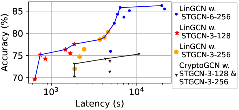
To bridge the research gap, in this paper, we propose LinGCN, an end-to-end policy-guided framework for non-linear reduction and polynomial replacement. This framework is designed to optimize deep Spatial-Temporal Graph Convolution Network (STGCN)-based models for HE-based inference. We conduct extensive experiments on the NTU-XVIEW [21] skeleton joint [22, 23, 24] dataset and compare our approach with CryptoGCN [12]. The pareto frontier comparison of accuracy-latency between LinGCN and CryptoGCN [12] demonstrates that LinGCN surpasses CryptoGCN [12] by over 5% accuracy under the same latency budget, and achieves a 14.2-fold latency reduction under the same accuracy constraint (~75% accuracy).

Our proposed framework, LinGCN, is principally influenced by two observations: the need to conserve levels in the CKKS scheme and the crucial role of synchronized linearization. In the CKKS scheme, deeper networks demand a larger polynomial degree, thereby increasing the latency of homomorphically encrypted operators. Non-linear layer pruning can mitigate this by reducing level consumption. However, unstructured non-linear pruning is insufficient; structural linearization becomes essential for effective level reduction, underscoring synchronized linearization’s significance in optimizing CKKS performance. We summarize our contributions as follows:

1. We present a differentiable structural linearization algorithm, paired with a parameterized discrete indicator function, which guides the structural polarization process. This methodology is co-trained with model weights until the optimization objective is attained. Our approach facilitates fine-grained node-level selection of non-linear locations, ultimately yielding a model with reduced multiplication levels.

2. We introduce a node-wise polynomial replacement policy utilizing a second-order trainable polynomial activation function. This process is further steered by an all-ReLU based teacher model employing a two-level distillation approach, thus promoting superior convergence.

3. We have engineered a corresponding HE solution that facilitates finer-grained operator fusion for node-wise activation functions. This development further mitigates multiplication level consumption during our HE-based inference process.

2 Background and Related Work

CKKS Homomorphic Encryption Scheme. The CKKS scheme [15], based on the ring learning with errors (RLWE) problem, allows arithmetic operations on encrypted fixed-point numbers. It provides configurable precision via encryption noise as natural error $e$ [25]. We denote the cyclotomic polynomial degree as $N$ and the polynomial coefficient modulus as $Q$, both cryptographic parameters. A ciphertext $ct$ encrypts a message $m$ with noise $e$ as $ct=m+e$ (mod $Q$). The CKKS scheme’s security level [26], measured in bits, suggests $2^{128}$ operations to break a $\lambda=128$ encryption. CKKS supports operations including ciphertext addition Add($ct_{1},ct_{2}$), ciphertext multiplication CMult($ct_{1},ct_{2}$), scalar multiplication PMult(ct , pt), rotation Rot(ct , k) and rescaling Rescale(ct). Scalar multiplication multiplies a ciphertext with plaintext, and rotation cyclically shifts the slot vector. For example, ${Rot(ct,k)}$ transforms $(v_{0},...,v_{N/2-1})$ into $(v_{k},...,v_{N/2-1},v_{0},...,v_{k-1})$. The level of a ciphertext ($L$), the number of successive multiplications it can undergo without bootstrapping, is reduced by the $Rescale$ operation after each multiplication. With the level-reduced target network, we do not consider using bootstrapping [27] in this work.

STGCN for Graph Dataset with Timing Sequence. The focus of this study revolves around the STGCN, a highly esteemed category of GCNs proposed by [4]. The STGCN model primarily employs two core operators, Spatial graph convolution (GCNConv) and Temporal convolution, designed to extract spatial and temporal information from input graph data, respectively. The Spatial convolution operation, as defined in Equation 1, precisely illustrates the process of extracting spatial information. In Equation 1, the variables $\bm{A}$, $\bm{D}$, $\bm{X}_{i}$, $\bm{W}_{i}$, and $\bm{X}_{i,\text{out}}$ correspond to the adjacent matrix, degree matrix, input feature, weight parameter, and output feature, respectively [4].

$$\bm{X}_{i,out}=\bm{D}^{-\frac{1}{2}}(\bm{A}+\bm{I})\bm{D}^{-\frac{1}{2}}\bm{X}_{i}\bm{W}_{i}$$ (1)

Related Work. CryptoNets [19] pioneered Privacy-Preserving Machine Learning (PPML) via Homomorphic Encryption (HE) but suffered from extended inference latency for large models. Subsequent studies, like SHE [28] which realizes realize the TFHE-based PPML, and those employing Multi-Party Computation (MPC) solutions[29, 30, 31], reduced latency but faced high communication overhead and prediction latency. Research like TAPAS [17] and XONN [32] compressed models into binary neural network formats, while studies like CryptoNAS [30], Sphynx [33], and SafeNet [34] used Neural Architecture Search (NAS) to find optimal architectures. Delphi [29], SNL [35], and DeepReduce [36] replaced ReLU functions with low order polynomial or linear functions to accelerate MPC-based Private Inference (PI). Nevertheless, these strategies proved suboptimal for homomorphic encrypted inference. Solutions like LoLa [20], CHET [37], and HEAR [38] sought to use ciphertext packing techniques but were not optimized for GCN-based models.

Threat Model. In line with other studies [12, 37, 39], we presume a semi-honest cloud-based machine learning service provider. The well-trained STGCN model’s weight, including adjacency matrices, is encoded as plaintexts in the HE-inference process. Clients encrypt data via HE and upload it to the cloud for privacy-preserving inference service. The server completes encrypted inference without data decryption or accessing the client’s private key. Finally, clients decrypt the returned encrypted inference results from the cloud using their private keys.

3 LinGCN Framework

3.1 Motivation

We present two pivotal observations that serve as the foundation for our LinGCN.

CKKS Based Encrypted Multiplication. As described in section 2, the message $m$ is scaled by a factor $\Delta=2^{p}$ before encoding, resulting in $\Delta m$. Any multiplicative operations square the ciphertext’s scale, including inherent noise $e$. The $Rescale$ operation reduces this scale back to $\Delta$ by modswitch [15], reducing $Q$ by $p$ bits and lowering the level, as depicted in Figure 2. When $Q\rightarrow q_{o}$ after $L$ multiplications and rescaling, the ciphertext’s multiplicative level reaches 0. At this stage, bootstrapping [12] is necessary for further multiplication, unless a higher $Q$ is used to increase the multiplicative level $L$.
Observation 1: Saving Level is Important in CKKS Scheme. Within a STGCN model, the graph embedding is encrypted with an initial polynomial degree, denoted as $N$, and a coefficient modulus, represented by $Q$. These factors are determined by the network’s multiplicative depth. As the multiplication depth increases, the coefficient modulus must also increase, subsequently leading to a higher polynomial degree $N$. To maintain a security level above a certain threshold (for example, 128-bit) in the face of deeper multiplicative depths, a larger $N$ is necessitated [37, 38, 12]. A larger $N$ inherently results in increased complexity in each homomorphic encryption operation such as Rot and CMult.

Figure 2: Top: Rescale decreases the ciphertext level. Bottom: Higher polynomial degree leads to longer HE operator’s latency.

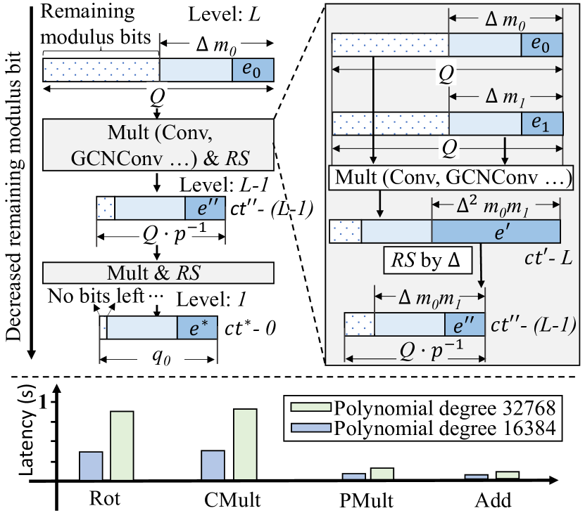
These operations are integral to the computation of convolution (Conv) and graph convolution (GCNConv). We present a comparative analysis of operator latency with differing polynomial degrees $N$ in Figure 2. Thus, it can be inferred that pruning certain operators to conserve levels not only diminishes the latency of the pruned operators but also reduces other operators’ latency.

Observation 2: Synchronized Linearization Matters. Our study mainly targets reducing multiplication depth in standard STGCN layers, comprising an initial spatial GCNConv operation, two non-linear operators, and a temporal convolution. Under the CKKS base HE scheme, each operator’s input needs synchronized multiplication depths, with any misalignment adjusted to the minimal depth. This is particularly vital for the GCNConv operator, while later node-wise separable operators enable structured non-linear reduction to boost computational efficiency.

Figure 3: Unstructured vs. structural linearization. Unstructured one doesn’t lead to effective level reduction.

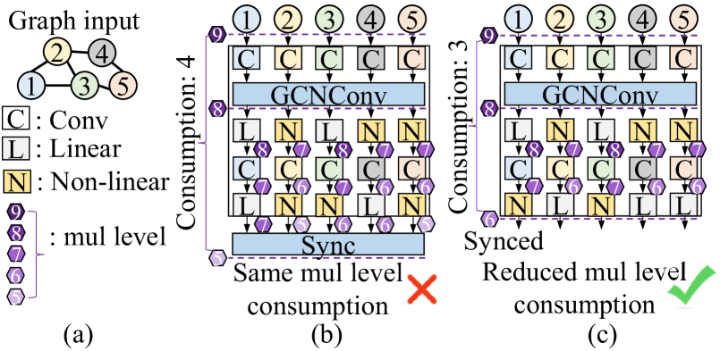
Unstructured non-linear reduction strategies, common in MPC setups like AutoReP [40], PASNet [41] SNL [35], RRNet [42], DELPHI [29], and SAFENet [43], prove suboptimal for homomorphic encrypted inference. Our example in Figure 3(b) illustrates node-wise unstructured non-linear reduction in an STGCN layer, leading to unsynchronized remaining multiplication depth budgets for nodes after the layer. This approach is ineffective in reducing levels consumption for homomorphic encrypted inference, emphasizing the necessity for a more structured non-linear reduction approach. To address the limitations of unstructured non-linear reduction, we propose a structured approach, illustrated in Figure 3(c), where we apply an equal level of non-linear reduction to each target node, reducing the overall multiplication depth. In contrast to CryptoGCN’s layer-wise pruning method [12], our scheme provides nodes with the flexibility to perform non-linear operations at preferred positions. This fine-grained, structural non-linear reduction may improve the non-linear reduced structure, potentially augmenting the efficiency and effectiveness of HE inference.

3.2 Learning for Structural Linearization

Problem Formulation. Our methodology is aimed at the node-wise structural dropping of non-linear operators within a given $L$-layered STGCN model $f_{W}$, parameterized by $W=\{W_{i}\}_{i=0}^{2L}$. This model maps the input $X_{0}\in R^{V\times C\times T}$ to the target $Y\in R^{d}$. Here, $V$, $C$, and $T$ represent the number of nodes, channels, and frames, respectively. The primary objective of our approach is to eliminate the non-linear operator (designated as $\sigma_{n}$) in a structured, node-wise manner. The ultimate aim is to achieve a reduced multiplication level while minimizing any resultant drop in model accuracy. This goal serves to optimize the efficiency of homomorphic encrypted inference for STGCN model.

We introduce an indicator parameter, denoted as $h$, to mark the node-wise non-linear operator dropping. The following conditions apply: (1) If $h_{i,k}=0$, the non-linear operator $\sigma_{n}$ is substituted by the linear function $f(x)=x$; (2) If $h_{i,k}=1$, the operator $\sigma_{n}$ is utilized. Here, $h_{i,k}$ signifies the $k_{th}$ node of the $i_{th}$ non-linear layer. The proposed node-wise non-linear indicator parameter $h_{i,k}$ facilitates the expression of the $i_{th}$ non-linear layer with partial linearization, as given by $X_{i,k}=h_{i,k}\odot\sigma_{n}(Z_{(i-1),k})+(1-h_{i,k})\odot Z_{(i-1),k}$. Here, $Z_{i-1}$ denotes the input of the $i_{th}$ non-linear layer. Consequently, the issue of structural linearization can be formulated as follows:

$$\begin{split}&\underset{W,h}{\text{argmin}}\mathcal{L}=\underset{W,h}{\text{argmin}}\ \ \ \mathcal{L}_{acc}(f_{W}(X_{0}),Y)+\mu\cdot\sum_{i=1}^{2L}||h_{i}||_{0}\\ &\text{subject to}\>\forall j,k\in[1,V],\ (h_{2i,j}+h_{2i+1,j})=(h_{2i,k}+h_{2i+1,k})\end{split}$$ (2)

In our formulation, $||h_{r}||0$ represents the $L_{0}$ norm or the count of remaining non-linear operators. $\mathcal{L}{acc}$ signifies cross-entropy loss, while $\mu$ is the $L_{0}$ norm penalty term in the linearization process. The second term of Eq. 2 poses a challenge due to its non-differentiability, stemming from zero norm regularization and additional constraints on the discrete indicator parameter $h_{i}$. Hence, this issue becomes difficult to handle using traditional gradient-based methods.

Differentiable Structural Linearization. To handle the non-differentiable discrete indicator parameter, we introduce a trainable auxiliary parameter, $h_{w}$, to denote its relative importance. However, the transformation from $h_{w}$ to the final indicator $h$ must comply with the structural constraint in Eq.2, ruling out simple threshold checks used in SNL [35]. Structural pruning methods [44, 45], useful for weight or neuron pruning, are ill-suited for our problem due to its exponential complexity arising from 2 non-linear selections of 25 nodes, and its distinct nature from weight or neuron pruning.

Algorithm 1 Structural Polarization.

0:  $h_{w}$: auxiliary parameter

0:  $h$: final indicator

1:  for $i=0$ to $L$ do

2:     $s_{h},s_{l}=0$ and $ind_{h},ind_{l}\leftarrow\emptyset$

3:     for $j=1$ to $V$ do

4:        if $h_{w(2i,j)}>h_{w(2i+1,j)}$ then

5:           $s_{h}\ +=\ h_{w(2i,j)}$, $s_{l}\ +=\ h_{w(2i+1,j)}$

6:           $ind_{h}\leftarrow(2i,j)$, $ind_{l}\leftarrow(2i+1,j)$

7:        else

8:           $s_{h}\ +=\ h_{w(2i+1,j)}$, $s_{l}\ +=\ h_{w(2i,j)}$

9:           $ind_{h}\leftarrow(2i+1,j)$, $ind_{l}\leftarrow(2i,j)$

10:        end if

11:     end for

12:     $h_{ind_{h}}=s_{h}>0$ and $h_{ind_{l}}=s_{l}>0$

13:  end for

To tackle this challenge, we propose a structural polarization forward process, detailed in Algorithm 1. The algorithm first ranks the relative importance of two auxiliary parameters ($h_{w(2i,j)}$ and $h_{w(2i+1,j)}$) for every $j_{th}$ node within the $i_{th}$ STGCN layer, obtaining the higher and lower values and their respective indices. We then sum each $i_{th}$ layer’s higher auxiliary parameter value into $s_{h}$, and lower auxiliary parameter value into $s_{l}$. Next, we conduct a threshold check of $s_{h}$ and assign the final polarization output of the indicator value into the corresponding locations of higher value indices, applying the same polarization for lower values. The proposed structural polarization enforces the exact constraint as given in Eq. 2, where each STGCN layer maintains a synchronized non-linear count across all nodes. The structural polarization is also capable of capturing the relative importance of the auxiliary parameter within each node and applying the proper polarization to every position, all with a complexity of only $O(V)$. Each STGCN layer retains the flexibility to choose all positions to conduct the non-linear operation, or just select one position for each node to conduct the non-linear operation, or opt not to perform the non-linear operation at all. This selection is based on the importance of their auxiliary parameters.

Despite its benefits, the structural binarization in Algorithm 1 is discontinuous and non-differentiable. To approximate its gradient, we use coarse gradients [46] via straight through estimation (STE), a good fit for updating $h_{w}$ and reflecting the optimization objective in Eq.2. Among various methods such as Linear STE[47], ReLU and clip ReLU STE [48], we adopt Softplus STE [49] due to its smoothness and recoverability discovered in [49], to update $h_{w}$ as follows:

$$\frac{\partial\mathcal{L}}{\partial h_{w(i,k)}}=\frac{\partial\mathcal{L}_{acc}}{\partial X_{i,k}}(\sigma_{n}(Z_{i-1})-Z_{i-1})\frac{\partial h_{i,k}}{\partial h_{w(i,k)}}+\mu\frac{\partial h_{i,k}}{\partial h_{w,(i,k)}},\ \ \frac{\partial h_{i,k}}{\partial h_{w(i,k)}}=Softplus(h_{w(i,k)})$$ (3)

The gradient of the auxiliary parameter, as displayed in Eq. 3, consists of two components: the gradient from the accuracy constraint and the gradient from the linearization ratio constraint. The gradient stemming from the accuracy constraint will be negative if it attempts to counteract the linearization process, thereby achieving a balance with the $L_{0}$ penalty term $\mu\cdot\sum_{i=1}^{2L}||h_{i}||_{0}$. The entirety of the linearization process is recoverable, which allows for the exploration of a near-optimal balance between accuracy and linearization ratio via the back-propagation process.

Figure 4: Overview of single layer STGCN with non-linear reduction and computation.

3.3 Learnable Polynomial Replacement with Teacher Guidance

CryptoNet [19] and DELPHI [29] suggest using quadratic functions $y=x^{2}$ as ReLU replacements for private inference. A second-order polynomial replacement  [50] $y=x^{2}+x$ for ReLU was proposed but resulted in decreased performance. CryptoGCN [12] uses a layer-wise trainable polynomial function $(ax^{2}+bx+c)$ for the STGCN model, but it suffers from significant accuracy loss and scalability problems. To tackle these issues, we offer a two-tiered strategy: node-wise trainable polynomial replacement and a distillation technique to facilitate the convergence of replacement.

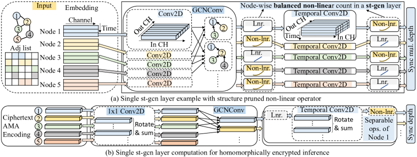
Node-wise Trainable Polynomial Replacement. In our HE setup (see Figure 4), each node can independently perform non-linear, convolution, and further non-linear operations without increasing the multiplication depth. We suggest using a node-wise trainable polynomial function as the non-linear function (see Eq. 4). To prevent gradient explosion from quadratic terms, we include a small constant $c$ to adjust the gradient scale of the $w_{2}$ parameter [41].

$$\sigma_{n}(x)=c\cdot w_{2}x^{2}+w_{1}x+b$$ (4)

Improved Convergence Through Distillation. Training a polynomial neural network from scratch often overfits, leading to accuracy loss [50, 12]. To counteract this, we recommend initially training a baseline ReLU model as the teacher, then transferring its knowledge to the polynomial student model to lessen accuracy degradation. The student model’s parameters are initialized from the teacher’s and polynomial function parameters start at $(w_{2}=0,w_{1}=1,b=0)$. To aid knowledge transfer, we use KL-divergence loss [51] and peer-wise normalized feature map difference penalty. The loss function for polynomial replacement is as follows:

$$\mathcal{L}_{p}=(1-\eta)\mathcal{L}_{CE}(f_{W,s}(X_{0}),Y)+\eta\mathcal{L}_{KL}(f_{W,s}(X_{0}),f_{W,t}(X_{0}))+\frac{\varphi}{2}\sum_{i=1}^{L}MSE(\frac{X_{i,s}}{||X_{i,s}||_{2}},\frac{X_{i,t}}{||X_{i,t}||_{2}})$$ (5)

In the above equation, $\eta$ is employed to balance the significance between the CE loss and the KL divergence loss components, while $\varphi$ acts as the penalty weight for the peer-wise feature map normalized $L_{2}$ distance term, analogous to the approach in [52].

3.4 Put it Together

The comprehensive workflow of our proposed LinGCN framework is outlined in Algorithm 2. Initially, we construct the student model, $M_{S}$, utilizing the parameters of the teacher model, $M_{T}$, and subsequently initialize the indicator auxiliary parameter $h_{w}$ for $M_{S}$. Following this, $M_{S}$ undergoes training iterations involving updates for structural linearization. Upon achieving convergence, the indicator function $h$ is fixed, and the ReLU function in $M_{S}$ is replaced with a polynomial function. Subsequently, we initialize $w_{poly}$ and train the final model using a combination of CE loss and the two-level distillation loss as defined in Eq. 5.

Algorithm 2 LinGCN Framework Workflow.

0:  Pretrain ReLU-based model $M_{T}$, linearization penalty $\mu$ and optim. $OP_{L}$, polynomial replacement optim. $OP_{P}$

0:  Level-reduced polynomial model

1:  Copy $M_{S}$ from $M_{T}$

2:  Initialize $h_{w}$ for $M_{S}$

3:  for Structural linearization iterations do

4:     Calculate $\mathcal{L}$ via Eq. 2 and Algorithm 1

5:     Update $W$ and $h_{w}$ through back propagation (Eq. 3) by minimizing $\mathcal{L}$ using $OP_{L}$

6:  end for

7:  Freeze $h_{w}$ and $h$

8:  Replace ReLU in $M_{s}$ with polynomial

9:  Initialize $w_{poly}$

10:  for Polynomial replacement iterations do

11:     Calculate $\mathcal{L}_{p}$ via Eq. 5

12:     Update $W$ through back propagation by minimizing $\mathcal{L}_{p}$ using $OP_{P}$

13:  end for

The resulting model output will feature structurally pruned node-wise polynomial functions, rendering it primed for the final stage of homomorphic encryption-based inference.

Further Operator Fusion to Save Level. Figure 4 shows an example of the single-layer STGCN structure generated by our LinGCN framework. The STGCN utilizes both input nodes information and aggregates them to generate output node features. We adopt the same AMA format [12] for GCNConv computation, as such, we are able to fuse the plaintext weights $c\cdot w_{2}$ of node-wise polynomial function into GCNConv layer and save one multiplication depth budget. Layer operators involve another temporal convolution layer and non-linear/linear layer, we can still fuse the plaintext weights $c\cdot w_{2}$ from the second polynomial function into the convolution operator and save the multiplication depth budget. As such, the ReLU-reduced example shown in Figure 4 only consumes 3 multiplication level of ciphertext as opposed to the original 4 multiplication depth budget. For the convolution operator, we adopt the same computation flow from [12, 38].

4 Experiment

4.1 Experiment Setting

HE Parameter Setting. We performed experiments with two sets of encryption parameters: one without and one with non-linear reduction. We used a scaling factor $\Delta=2^{33}$ in both cases to ensure comparable accuracy. This scaling consumes 33 bits from the ciphertext modulus $Q$ per level. Without non-linear reduction, a 3-layer STGCN network needs 14 levels, and a 6-layer network needs 27. For a security level of 128-bit, we set $Q$ to 509 (932) and the polynomial degree $N$ to $2^{15}(2^{16})$ for 3 (6) layers STGCN network. In the non-linear reduction case, the total level count ranges from 14 to 9 for 3-layer, and 27 to 16 for 6-layer networks. With the reduced models, we can use smaller Q and $N$ while maintaining 128-bit security. Specifically, we set $Q$ to 410 to 344 and $N$ to $2^{14}$ for the 3-layer network (from 3 non-linear reduced), and $Q$ to 767 to 569 and $N$ to $2^{15}$ for the 6-layer network (starting from 5 non-linear reduced).

Experiment Dataset. The NTU-RGB+D dataset [21], the largest available with 3D joint annotations for human action recognition, is utilized in our study. With 56,880 action clips in 60 classes, each is annotated with $(X,Y,Z)$ coordinates of 25 joints (nodes) per subject. We chose the NTU-cross-View (NTU-XView) benchmark given its representativeness as a human skeleton joint dataset, containing 37,920 training and 18,960 evaluation clips. For a thorough evaluation, 256 frames were used from each clip, resulting in a $2\times 3\times 256\times 25$ input tensor for two individuals each with 3 channels.

Baseline Model. Our experiment runs on 8*A100 GPU server, and uses the state-of-the-art STGCN architecture for human action recognition, which combines GCN and CNN. We tested three configurations: STGCN-3-128, STGCN-3-256, and STGCN-6-256, where the first number represents the layer count, and the second the last STGCN layer’s channel count. These networks contain a stack of three or six STGCN layers, followed by a global average pooling layer and a fully-connected layer. They were trained for 80 epochs using SGD, with a mini-batch size of 64, a momentum of 0.9, weight decay of $10^{-4}$, and dropout 0.5. The initial learning rate (LR) was 0.1, with a decay factor of 0.1 at the 10th and 50th epochs. The baseline accuracy of models can also be found in Table 1.

Table 1: All ReLU based model architecture and accuracy

Model	Layer-wise number of channel configuration	Accuracy (%)
STGCN-3-128	3-64-128-128	80.64
STGCN-3-256	3-128-256-256	82.80
STGCN-6-256	3-64-64-128-128-256-256	84.52

LinGCN Algorithm Setting. In our LinGCN algorithm, we used the baseline model from Table 1 as the teacher model in Algorithm 2. For structural linearization, we used SGD optimizer with learning rate (LR) 0.01 for both weight and auxiliary parameters. The $L_{0}$ norm penalty $\mu$ was varied from 0.1 to 10 for desired linearized layers, over 25 epochs. Then, ReLU was replaced with a second-order polynomial in the polynomial replacement iterations. We set scaling factor $c$ at 0.01, parameters $\eta$ and $\varphi$ at 0.2 and 200 respectively. This process took 90 epochs, with SGD optimizer and initial LR of 0.01, decaying by a factor of 0.1 at the $40th$ and $80th$ epochs.

Private Inference Setup. Our experiments used an AMD Ryzen Threadripper PRO 3975WX machine, single threaded. The RNS-variant of the CKKS scheme [53] was employed using Microsoft SEAL version 3.7.2 [54]. We adopted the Adjacency Matrix-Aware (AMA) data formatting from CryptoGCN [12] to pack input graph data and performed GCNConv layer inference via multiplying with sparse matrices $A_{i}$ split from the adjacency matrix $A$. The temporal convolution operation was optimized using the effective convolution algorithm from [38, 12, 55]. The computation for the global average pooling layer and fully-connected layer also follows the SOTA [38, 12].

Table 2: STGCN-3-128 comparison

Model	STGCN-3-128
Methods	Non-linear layers	Test acc (%)	Latency (s)
LinGCN	6	77.55	1856.95
LinGCN	5	75.48	1663.13
LinGCN	4	76.33	1458.95
LinGCN	3	74.27	850.22
LinGCN	2	75.16	741.55
LinGCN	1	69.61	642.06
CryptoGCN	6	74.25	4273.89
CryptoGCN	5	73.12	1863.95
CryptoGCN	4	70.21	1856.36

Table 3: STGCN-3-256 comparison

Model	STGCN-3-256
Methods	Non-linear layers	Test acc (%)	Latency (s)
LinGCN	6	80.29	4632.05
LinGCN	5	79.07	4166.12
LinGCN	4	78.59	3699.49
LinGCN	3	76.41	2428.88
LinGCN	2	74.74	2143.46
LinGCN	1	71.98	1873.40
CryptoGCN	6	75.31	10580.41
CryptoGCN	5	73.78	4850.93
CryptoGCN	4	71.36	4831.93

4.2 Experiment Result and Comparison

LinGCN Outperforms CryptoGCN [12]. The proposed LinGCN algorithm demonstrates superior performance compared to CryptoGCN [12]. The STGCN-3-128 and STGCN-3-256 models, which are the basis of this comparison, share the same backbone as those evaluated in CryptoGCN [12]. Hence, we have undertaken a comprehensive cross-work comparison between the LinGCN framework and CryptoGCN [12]. The latter employs a heuristic algorithm for layer-wise activation layer pruning, which necessitates a sensitivity ranking across all layers. This approach, however, proves to be ineffective, leading to significant accuracy drops as the number of pruned activation layers increases.
Comparative results between LinGCN and CryptoGCN [12] are provided in Table 3 and Table 3. In the context of LinGCN, the number of non-linear layers presented in the table represents the effective non-linear layers post-structural linearization. For the STGCN-3-128 and STGCN-3-256 models, LinGCN yielded an accuracy of 77.55% and 80.28% respectively for the baseline 6 non-linear layers model, exceeding CryptoGCN [12] by 3.3% and 4.98%. This outcome signifies the superiority of our proposed teacher-guided node-wise polynomial replacement policy over the naive layer-wise polynomial replacement provided in CryptoGCN [12].

Importantly, the LinGCN model for the 6 non-linear layers employs a more fine-grained node-wise polynomial function, which is fused into the preceding Conv or GCNConv layers. Thus, the encryption level required is lower than that of CryptoGCN [12], resulting in reduced latency. When considering non-linear layer reduction performance, LinGCN experiences only a 1.2 to 1.7 % accuracy decline with a 2 effective non-linear layer reduction, whereas CryptoGCN [12] displays approximately 4% accuracy degradation when pruned for 2 non-linear layers. Remarkably, LinGCN achieves an accuracy improvement of more than 6% over CryptoGCN [12] for models with 4 non-linear layers. Even in models with only 2 non-linear layers, LinGCN exhibits exceptional accuracy (75.16% and 74.74%). While this accuracy aligns with the performance of 6 non-linear layer models in CryptoGCN [12], LinGCN significantly outperforms it in terms of private inference latency, providing more than a five-fold reduction compared to CryptoGCN [12].

Figure 5: STGCN-3-256 structural linearization

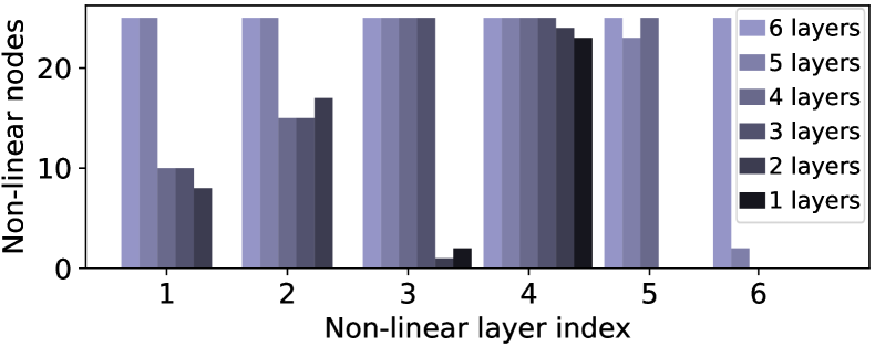
Non-linear Layer Sensitivity. We conduct a sensitivity analysis on the STGCN-3-256 model to investigate the effect of non-linear layers. The results are displayed in Figure 5, wherein the $i$ layers in the figure represent the remaining effective non-linear layers in the model, and every $2i-1$ and $2i$ exhibit a total number of non-linear nodes summing up to an integer multiple of 25. During the automatic structural linearization process, the gradient propagation is orchestrated to strike a balance between two goals: (i) preserving the feature structural information at the deeper layers, and (ii) mitigating the over-smoothing effect [56] resulting from the deep linearized GCN layers. Consequently, the middle 4th layer’s nonlinearity is most important within the STGCN model.

Table 4: LinGCN for STGCN-6-256 model.

Model	STGCN-6-256
Methods	Non-linear layers	Test acc (%)	Latency (s)
LinGCN	12	85.47	21171.80
LinGCN	11	86.24	19553.96
LinGCN	7	85.08	8186.35
LinGCN	5	83.64	7063.51
LinGCN	4	85.78	6371.39
LinGCN	3	84.28	5944.81
LinGCN	2	82.27	5456.12
LinGCN	1	75.93	4927.26

LinGCN is Scalable. Beyond the evaluation of the 3-layer model, we also apply our LinGCN to a 6-layer STGCN-6-256 model, which no prior work evaluated, maintaining the same settings to assess the trade-off between accuracy and latency. An intriguing finding is that the teacher-guided full polynomial replacement not only maintains model performance but also surpasses the accuracy of the teacher baseline by 0.95%, achieving an accuracy of 85.47%. This suggests that the STGCN model equipped with a smooth polynomial activation function may enhance model expressivity. Experiments reveal a significant redundancy in the non-linear layers of the STGCN-6-256 model, as it exhibits no accuracy degradation up to the reduction of 8 non-linear layers. When the pruning extends to 10 non-linear layers, the accuracy experiences a slight dip of 3.2% compared to the non-reduction one.

Pareto Frontier of LinGCN. Figure 1 compares the Pareto frontier between LinGCN and CryptoGCN [12], showing LinGCN consistently surpassing CryptoGCN by at least 4% in accuracy across all latency ranges. As latency constraints ease (around 6000s), LinGCN’s accuracy notably increases, improving by roughly 10% over CryptoGCN. Impressively, LinGCN maintains an accuracy of 75.16% while achieving a private inference latency of 742s, making it 14.2 times faster than CryptoGCN.

4.3 Abalation Studies

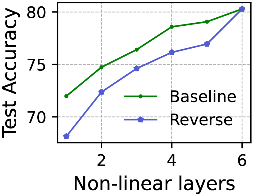
Non-linear Reduction & Replacement Sequence matters. Our LinGCN algorithm employs a sequence of non-linear reduction and polynomial replacement, proving more efficacious in terms of search space convergence compared to the inverse sequence of polynomial replacement followed by non-linear reduction. The reasoning behind this lies in the possibility that the polynomial replacement process may produce a model optimized for a given architecture, hence subsequent changes to the architecture, such as non-linear reduction, could lead to significant accuracy degradation. Keeping all other parameters constant and merely altering the replacement sequence, we present the accuracy evaluation results of STGCN-3-256 model in Figure 6a. As depicted in the figure, the sequence of polynomial replacement followed by non-linear reduction incurs an accuracy degradation exceeding 2% compared to the baseline sequence across all effective non-linear layer ranges.

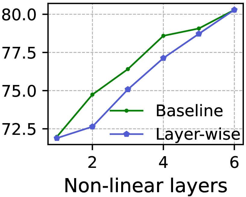
LinGCN Outperforms Layer-wise Non-linear Reduction. A significant innovation in our LinGCN framework is the structural linearization process. This process allows nodes to determine their preferred positions for non-linearities within a single STGCN layer, as opposed to enforcing a rigorous constraint to excise the non-linearity across all nodes. This less restrictive approach yields a more detailed replacement outcome compared to the layer-wise non-linear reduction. To demonstrate the impact of this method, we kept all other parameters constant for of STGCN-3-256 model, altering only the structural linearization to layer-wise linearization, and subsequently evaluated the model’s accuracy, as shown in Figure 6b. The results indicate that layer-wise linearization results in a 1.5% decrease in accuracy compared to structural linearization within the range of 2 to 5 effective non-linear layers. This demonstrates the effectiveness of the proposed structural linearization methodology.

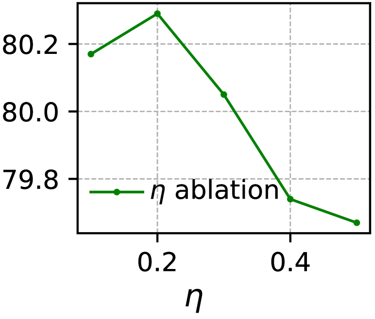
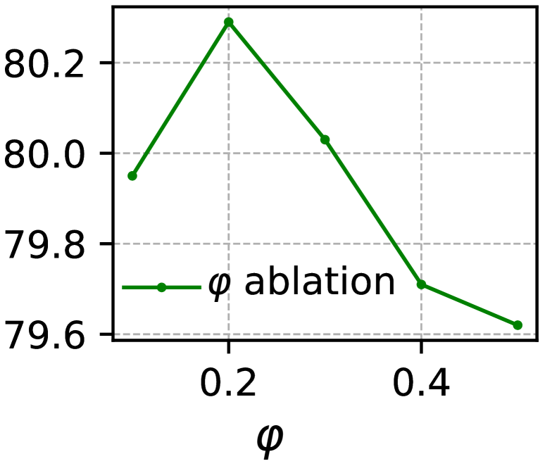
Distillation Hyperparameter Study. In prior experiments, we kept $\eta$ and $\varphi$ at 0.2 and 200 respectively. To assess their influence during distillation, we tested $\eta$ and $\varphi$ across a range of values while distilling the STGCN-3-256 model with 6 non-linear layers. We test $\eta\in[0.1,0.2,0.3,0.4,0.5]$ and $\varphi\in[100,200,300,400,500]$. Notably, we maintained $\varphi=200$ and $\eta=0.2$ for the respective $\eta$ and $\varphi$ ablations. The study, shown in Figure 6c and Figure 6d, confirms that $\eta=0.2$ and $\varphi=200$ yield optimal accuracy, and larger penalties might lower accuracy due to mismatch with the teacher model. This study thus justifies our selection of the $\eta$ and $\varphi$.

Table 5: LinGCN for Flickr dataset.

Num. of nonlinear layers in GCN layers	Accuracy (val/test, %)	Latency (s)
6	0.5281/0.5275	4290.93
2	0.5247/0.5266	2740.94
1	0.5269/0.5283	2525.80

LinGCN Generalize to Other Dataset. Without loss of generality, we extended our evaluation on Flickr [57] dataset, which is a representative node classification dataset widely used in GNN tasks.It consists of 89,250 nodes, 989,006 edges, and 500 feature dimensions. This dataset’s task involves categorizing images based on descriptions and common online properties. For the security setting, we assume that node features are user-owned and the graph adjacency list is public. The Flickr dataset has a larger adjacent list but smaller feature dimension compared to the NTU-XVIEW dataset. We utilize three GCN layers with 256 hidden dimensions. Each GCN layer has similar structure as STGCN backbone architecture and has two linear and nonlinear layers. We conduct full-batch GCN training to obtain ReLU-based baseline model accuracies of 0.5492/0.5521 for validation/test dataset. We obtain the accuracy/latency tradeoff detailed in the Table 5. LinGCN framework substantially diminishes the number of effective nonlinear layers, which leads to 1.7 times speedup without much accuracy loss.

(a)

(b)

(c)

(d)

Figure 6: Ablation study for (a) Replacement sequence, (b) node-wise vs. layer-wise linearization. (c) $\eta$: KL divergence distillation parameter (d) $\varphi$: feature map distance distillation parameter.

5 Discussion and Conclusion

Recent advancements in MLaaS (Machine Learning as a Service) have primarily centered on accelerating plaintext inference [58, 59, 60, 61, 62, 63, 64, 65, 66, 67, 68, 69, 70, 71, 72, 73, 49, 74, 75, 76, 77, 78, 79, 80]. Some initiatives emphasize enhancing plaintext training speeds [81, 82, 83, 84, 85, 86, 87, 88, 89, 90, 91]. Additionally, there’s an increasing focus on federated learning to ensure the confidentiality of training datasets [92, 93, 94] and safeguarding the privacy of model providers [95].

Our LinGCN optimizes HE-based GCN inference by reducing multiplication levels through a differentiable structural linearization algorithm and a compact node-wise polynomial replacement policy, both guided by a two-level distillation from an all-ReLU teacher model. Additionally, we improve HE solutions for GCN private inference, enabling finer operator fusion for node-wise activation functions. LinGCN outperforms CryptoGCN by 5% in accuracy and reducing latency by 14.2 times at ~75% accuracy, LinGCN sets a new state-of-the-art performance for private STGCN model inference. In the future, we will expand the proposed algorithm on other neural network domains and applications, such as CNN based medical image.

Appendix A Appendix

A.1 HE encoding with AMA format

Prior to encoding input data into polynomials, it is necessary to map the four-dimensional tensor $X\in R^{B\times C\times T\times J}$ to a one-dimensional vector in $R^{N/2}$ using the AMA format, as proposed in [12]. This transformation allows for more efficient execution of STGCN forward-computation in the HE domain. Below, we present the definition of the $Vec$ function employed to map tensor $X$ to a vector in $R^{N/2}$:

$$\begin{split}Vec(X)=y_{j}&=(y_{0,j},\dots,y_{i,j},\dots,y_{N/2,j})\in R^{N/2}\\ \textit{s.t. }y_{i,j}&=X_{((i\textit{ mod }T)\%B)\times(i\textit{ mod }B\cdot T)\times(i\textit{ \% }T)\times j}\\ &j\in J\end{split}$$ (6)

Following the mapping process, the vectors $y_{j}$ are encoded into polynomials with degree $N$ and subsequently encrypted into ciphertext $ct_{j}$, as detailed in [53]. In this study, when N is set to $2^{16}$, all tensors, including intermediate tensors, can be encrypted and packed into 25 ciphertexts, which corresponds to the number of nodes. For cases where $N=2^{15}$ ($2^{14}$) the number of ciphertexts is 50(100). By selecting an appropriate value for N, the encryption and packing processes can be optimized to maintain performance and efficiency.

A.2 HE Setting Details

In Table 6, we furnish comprehensive details regarding the HE inference parameters. Specifically, i-STGCN-3 denotes a 3-layer STGCN model with i effective non-linear layers, while i-STGCN-6 signifies a 6-layer STGCN model with i effective non-linear layers. In this context, N represents the polynomial degree, and Q corresponds to the coefficient modulus.

To guarantee computation precision utilizing a one-time rescale operation, we assign the scale factor $p$ for both ciphertext and plaintext to $2^{33}$. This allocation results in a reduction of the current Q of ciphertext by p bits. This setup ensures that the overall performance and accuracy conform to the desired criteria while capitalizing on the security and resilience advantages conferred by HE.

Table 6: HE parameter settings in detail.

Model	Encryption Parameters				Mult
	N	Q	p	$q_{0}$	Level
6-STGCN-3	32768	509	33	47	14
5-STGCN-3	32768	476	33	47	13
4-STGCN-3	32768	443	33	47	12
3-STGCN-3	16384	410	33	47	11
2-STGCN-3	16384	377	33	47	10
1-STGCN-3	16384	344	33	47	9
12-STGCN-6	65536	932	33	41	27
11-STGCN-6	65536	899	33	41	26
7-STGCN-6	32768	767	33	41	22
5-STGCN-6	32768	701	33	41	20
4-STGCN-6	32768	668	33	41	19
3-STGCN-6	32768	635	33	41	18
2-STGCN-6	32768	602	33	41	17
1-STGCN-6	32768	569	33	41	16

A.3 HE inference on GCNConv and Temporal-Conv Layer

Upon obtaining the AMA-packed ciphertexts $ct_{j}$, the adjacency matrix multiplication $A\cdot X$ can be decomposed into a series of plaintext multiplications, PMult, in the HE domain. This decomposition accelerates HE-inference without necessitating rotations. Furthermore, the subsequent temporal convolution is performed solely on the temporal dimension $T$, utilizing $1\times 9$ kernels.

$$ct_{k}^{\prime}=A\cdot X=\sum_{i=1}^{m}ct_{k}A_{i}=\sum_{i=1}^{m}\sum_{k=1}^{J}PMult(ct_{i_{k}},a_{i_{k}k})$$ (7)

The AMA-packed ciphertexts allow for natural temporal convolution by single-node ciphertext $ct_{j}$, facilitating independent computation. This approach results in a ReLU-reduction design through structural pruning of ReLUs. The primary constraint to consider in this context is ensuring that the level consumption of each ciphertext remains equal prior to the GCNConv layer (node aggregation).

A.4 Further Detail of Operator Fusion

During the HE-inference process, employing weight fusion conserves the multiplicative depth, consequently reducing the ciphertext level budget. For instance, batch normalization, defined by an affine transformation $a^{\prime}x+b^{\prime}$, and a polynomial activation function, defined by $(ax+b)^{2}+c$, can be readily fused into the corresponding temporal convolution layer $wx+b^{\prime\prime}$ with the function $w(a(a^{\prime}x+b^{\prime})+b)+b^{\prime\prime}=(w\cdot a\cdot a^{\prime})x+ab^{\prime}+wb+b^{\prime\prime}$. As a result, three consecutive multiplications are consolidated into a single multiplication (pre-computing $w\cdot a\cdot a^{\prime}$), thereby reducing the level consumption of ciphertext from 4 to 2 ($1\times 9$ convolution, batch normalization, and polynomial activation).

Table 7: Comparison of latency breakdown between the non-reduced model with optimized model.

Model	HE Operators latency (s)				Total Latency	Speedup
	Rot	PMult	Add	CMult	(s)	($\times$)
6-STGCN-3-128	1336.25	378.25	99.65	37.45	1851.60	-
2-STGCN-3-128	392.21	266.13	68.90	14.31	741.55	2.50
6-STGCN-3-256	2641.09	1508.19	397.17	74.90	4621.36	-
2-STGCN-3-256	777.68	1062.21	274.96	28.63	2143.47	2.16
12-STGCN-6-256	18955.09	1545.09	396.23	275.39	21171.80	-
2-STGCN-6-256	4090.08	1006.79	244.19	115.05	5456.12	3.88

Analogous to the temporal-convolutional layer, the same fusion strategies can be applied to the polynomial activation and batch normalization of the GCNConv layer. Utilizing AMA-packed ciphertexts, the node aggregation in GCNConv is translated as depicted in Equation 7, where each ciphertext carries out scalar multiplication with the plaintext of matrix elements $a_{i_{k},k}$. Consequently, these plaintext matrix elements $a_{i_{k},k}$ are fused with the primary $1\times 1$ convolutional kernels to conserve the multiplicative level, reducing the total level consumption of the GCNConv layer from 4 to 2 ($1\times 1$ convolution, adjacency matrix multiplication, batch normalization, and polynomial activation).

A.5 Operator latency breakdown

Table 7 presents a comprehensive operator latency breakdown encompassing Rot, PMult, Add, and CMult operations. The designation i-STGCN-3-128 refers to an STGCN-3-128 model with i residual non-linear layers. As indicated in the table, the non-linear reduction contributes to a significant reduction in latency. By leveraging a smaller polynomial degree N, the overall latency experiences substantial improvement.

A.6 More Training Details and Insight

(a)

(b)

(c)

(d)

(e)

(f)

Figure 7: Polynomial replacement training curves for (a) 6-STGCN-3-128 (b) 5-STGCN-3-128 (c) 4-STGCN-3-128 (d) 3-STGCN-3-128 (e) 2-STGCN-3-128 (f) 1-STGCN-3-128

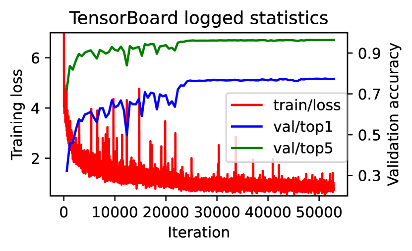
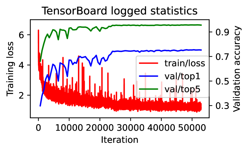
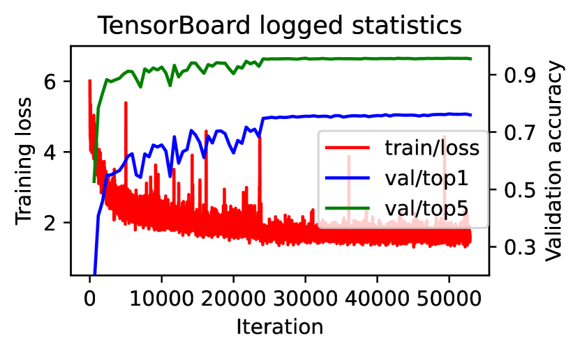
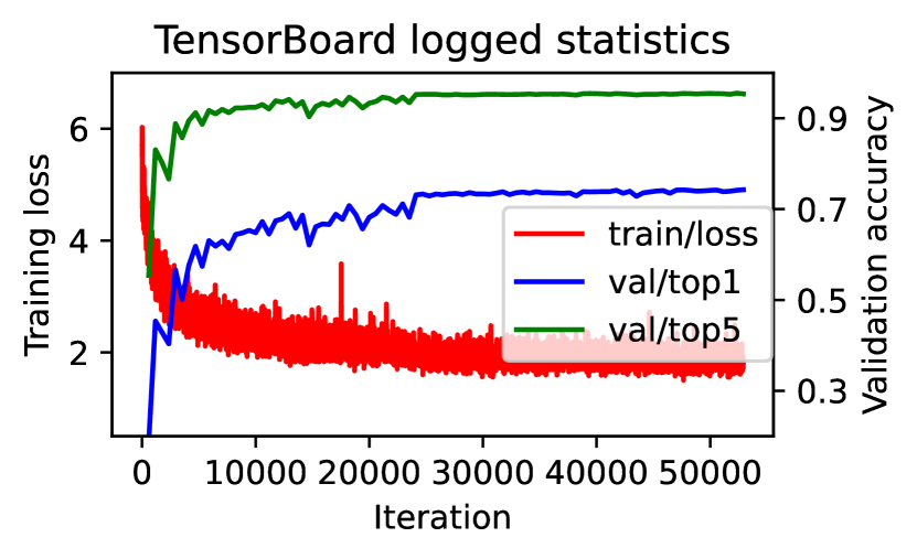
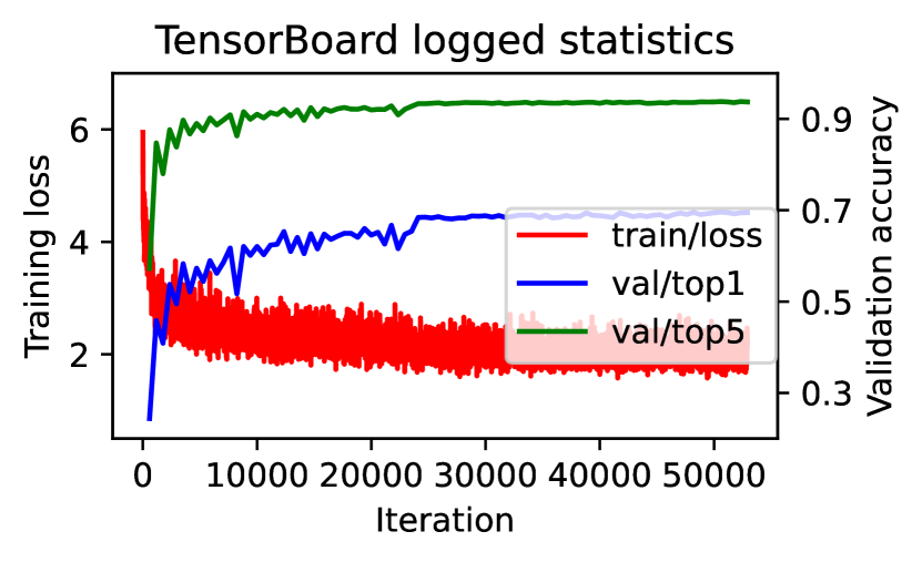
In this section, we present the training curves for the STGCN-3-256 model, which employs 6 to 1 effective second-order polynomial (non-linear) layers. Figures 7(a) through Figure 7(f) depict the training curve progression. During the training process, we utilized mixed-precision training for the polynomial model, which led to occasional instability in some iterations, as evidenced by spikes in the loss values. Nevertheless, the training process demonstrated rapid recovery following such loss spikes.

(a)

(b)

(c)

Figure 8: Polynomial replacement training curves for (a) 12-STGCN-6-256 (b) 4-STGCN-6-256 (c) 2-STGCN-6-256

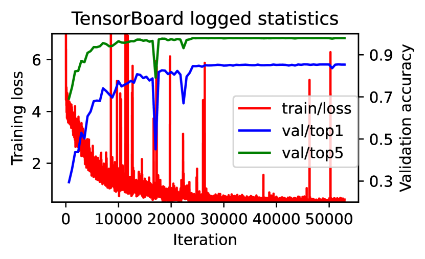
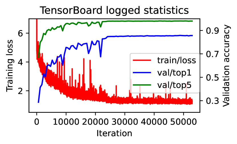
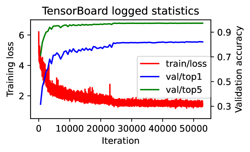
As demonstrated in training curve, a smaller number of second-order polynomial (non-linear) layers contribute to a more stable training process and facilitate smoother convergence. This finding explains the enhanced performance of the STGCN-6-256 model, which features a reduced number of non-linear layers, as compared to the full-polynomial model baseline.

To substantiate our hypothesis, we plot the polynomial replacement training curve for the STGCN-6-256 model in Figure 8. The training curves for 12 effective non-linear layers (12-STGCN-6-256), four effective non-linear layers (4-STGCN-6-256), and two effective non-linear layers (2-STGCN-6-256) are presented. As the number of non-linear layers increases, the model achieves greater expressivity; however, the polynomial replacement process becomes increasingly unstable. Consequently, for the STGCN-6-256 model with only 4 non-linear layers, a more stable replacement process facilitates better convergence, ultimately leading to improved accuracy performance.

References

- [1] Weijing Shi and Raj Rajkumar. Point-gnn: Graph neural network for 3d object detection in a point cloud. In CVPR, pages 1711–1719, 2020.
- [2] Weiwei Jiang and Jiayun Luo. Graph neural network for traffic forecasting: A survey. Expert Systems with Applications, page 117921, 2022.
- [3] Chenyang Si, Ya Jing, Wei Wang, Liang Wang, and Tieniu Tan. Skeleton-based action recognition with spatial reasoning and temporal stack learning. In Proceedings of the European conference on computer vision (ECCV), pages 103–118, 2018.
- [4] Sijie Yan, Yuanjun Xiong, and Dahua Lin. Spatial temporal graph convolutional networks for skeleton-based action recognition. In Thirty-second AAAI conference on artificial intelligence, 2018.
- [5] Shiwen Wu, Fei Sun, Wentao Zhang, Xu Xie, and Bin Cui. Graph neural networks in recommender systems: a survey. ACM Computing Surveys (CSUR), 2020.
- [6] Pietro Bongini et al. Molecular generative graph neural networks for drug discovery. Neurocomputing, 450:242–252, 2021.
- [7] Anuroop Sriram et al. Towards training billion parameter graph neural networks for atomic simulations. ArXiv, abs/2203.09697, 2022.
- [8] Daniel Manu et al. Co-exploration of graph neural network and network-on-chip design using automl. In Proceedings of the 2021 on Great Lakes Symposium on VLSI, pages 175–180, 2021.
- [9] Rex Ying et al. Graph convolutional neural networks for web-scale recommender systems. KDD ’18, 2018.
- [10] Rong Zhu et al. Aligraph: A comprehensive graph neural network platform. KDD ’19, 2019.
- [11] Ling Liang, Jilan Lin, Zheng Qu, Ishtiyaque Ahmad, Fengbin Tu, Trinabh Gupta, Yufei Ding, and Yuan Xie. Spg: Structure-private graph database via squeezepir. Proceedings of the VLDB Endowment, 16(7):1615–1628, 2023.
- [12] Ran Ran, Wei Wang, Quan Gang, Jieming Yin, Nuo Xu, and Wujie Wen. Cryptogcn: Fast and scalable homomorphically encrypted graph convolutional network inference. Advances in Neural Information Processing Systems, 35:37676–37689, 2022.
- [13] Le Trieu Phong, Yoshinori Aono, Takuya Hayashi, Lihua Wang, and Shiho Moriai. Privacy-preserving deep learning: Revisited and enhanced. In Applications and Techniques in Information Security: 8th International Conference, ATIS 2017, Auckland, New Zealand, July 6–7, 2017, Proceedings, pages 100–110. Springer, 2017.
- [14] Ligeng Zhu, Zhijian Liu, and Song Han. Deep leakage from gradients. Advances in neural information processing systems, 32, 2019.
- [15] Jung Hee Cheon, Andrey Kim, Miran Kim, and Yongsoo Song. Homomorphic encryption for arithmetic of approximate numbers. In International Conference on the Theory and Application of Cryptology and Information Security, pages 409–437. Springer, 2017.
- [16] Zvika Brakerski, Craig Gentry, and Vinod Vaikuntanathan. (leveled) fully homomorphic encryption without bootstrapping. ACM Transactions on Computation Theory (TOCT), 6(3):1–36, 2014.
- [17] Amartya Sanyal, Matt Kusner, Adria Gascon, and Varun Kanade. Tapas: Tricks to accelerate (encrypted) prediction as a service. In International Conference on Machine Learning, pages 4490–4499. PMLR, 2018.
- [18] Florian Bourse, Michele Minelli, Matthias Minihold, and Pascal Paillier. Fast homomorphic evaluation of deep discretized neural networks. In Advances in Cryptology–CRYPTO 2018: 38th Annual International Cryptology Conference, Santa Barbara, CA, USA, August 19–23, 2018, Proceedings, Part III 38, pages 483–512. Springer, 2018.
- [19] Ran Gilad-Bachrach, Nathan Dowlin, Kim Laine, Kristin Lauter, Michael Naehrig, and John Wernsing. Cryptonets: Applying neural networks to encrypted data with high throughput and accuracy. In International conference on machine learning, pages 201–210. PMLR, 2016.
- [20] Alon Brutzkus, Ran Gilad-Bachrach, and Oren Elisha. Low latency privacy preserving inference. In International Conference on Machine Learning, pages 812–821. PMLR, 2019.
- [21] Amir Shahroudy, Jun Liu, Tian-Tsong Ng, and Gang Wang. Ntu rgb+d: A large scale dataset for 3d human activity analysis. In Proceedings of the IEEE conference on computer vision and pattern recognition, pages 1010–1019, 2016.
- [22] Ke Sun, Bin Xiao, Dong Liu, and Jingdong Wang. Deep high-resolution representation learning for human pose estimation. In Proceedings of the IEEE/CVF conference on computer vision and pattern recognition, pages 5693–5703, 2019.
- [23] Kaiming He, Georgia Gkioxari, Piotr Dollár, and Ross Girshick. Mask r-cnn. In Proceedings of the IEEE international conference on computer vision, pages 2961–2969, 2017.
- [24] Zhe Cao, Tomas Simon, Shih-En Wei, and Yaser Sheikh. Realtime multi-person 2d pose estimation using part affinity fields. In Proceedings of the IEEE conference on computer vision and pattern recognition, pages 7291–7299, 2017.
- [25] Kim Laine. Simple encrypted arithmetic library (seal) manual, 2017.
- [26] Melissa Chase, Hao Chen, Jintai Ding, Shafi Goldwasser, Sergey Gorbunov, Jeffrey Hoffstein, Kristin Lauter, Satya Lokam, Dustin Moody, Travis Morrison, et al. Security of homomorphic encryption. HomomorphicEncryption. org, Redmond WA, Tech. Rep, 2017.
- [27] Craig Gentry. A fully homomorphic encryption scheme. Stanford university, 2009.
- [28] Ilaria Chillotti, Nicolas Gama, Mariya Georgieva, and Malika Izabachène. Tfhe: fast fully homomorphic encryption over the torus. Journal of Cryptology, 33(1):34–91, 2020.
- [29] Pratyush Mishra, Ryan Lehmkuhl, Akshayaram Srinivasan, Wenting Zheng, and Raluca Ada Popa. Delphi: A cryptographic inference service for neural networks. In 29th USENIX Security Symposium (USENIX Security 20), pages 2505–2522, 2020.
- [30] Zahra Ghodsi, Akshaj Kumar Veldanda, Brandon Reagen, and Siddharth Garg. Cryptonas: Private inference on a relu budget. Advances in Neural Information Processing Systems, 33:16961–16971, 2020.
- [31] Brian Knott, Shobha Venkataraman, Awni Hannun, Shubho Sengupta, Mark Ibrahim, and Laurens van der Maaten. Crypten: Secure multi-party computation meets machine learning. Advances in Neural Information Processing Systems, 34:4961–4973, 2021.
- [32] M Sadegh Riazi, Mohammad Samragh, Hao Chen, Kim Laine, Kristin Lauter, and Farinaz Koushanfar. XONN:XNOR-based oblivious deep neural network inference. In 28th USENIX Security Symposium (USENIX Security 19), pages 1501–1518, 2019.
- [33] Minsu Cho, Zahra Ghodsi, Brandon Reagen, Siddharth Garg, and Chinmay Hegde. Sphynx: Relu-efficient network design for private inference. arXiv preprint arXiv:2106.11755, 2021.
- [34] Qian Lou, Yilin Shen, Hongxia Jin, and Lei Jiang. Safenet: A secure, accurate and fast neural network inference. In International Conference on Learning Representations, 2020.
- [35] Minsu Cho, Ameya Joshi, Brandon Reagen, Siddharth Garg, and Chinmay Hegde. Selective network linearization for efficient private inference. In International Conference on Machine Learning, pages 3947–3961. PMLR, 2022.
- [36] Nandan Kumar Jha, Zahra Ghodsi, Siddharth Garg, and Brandon Reagen. Deepreduce: Relu reduction for fast private inference. In International Conference on Machine Learning, pages 4839–4849. PMLR, 2021.
- [37] Roshan Dathathri, Olli Saarikivi, Hao Chen, Kim Laine, Kristin Lauter, Saeed Maleki, Madanlal Musuvathi, and Todd Mytkowicz. Chet: an optimizing compiler for fully-homomorphic neural-network inferencing. In Proceedings of the 40th ACM SIGPLAN Conference on Programming Language Design and Implementation, pages 142–156, 2019.
- [38] Miran Kim, Xiaoqian Jiang, Kristin Lauter, Elkhan Ismayilzada, and Shayan Shams. Secure human action recognition by encrypted neural network inference. Nature communications, 13(1):1–13, 2022.
- [39] Miran Kim, Xiaoqian Jiang, Kristin Lauter, Elkhan Ismayilzada, and Shayan Shams. Hear: Human action recognition via neural networks on homomorphically encrypted data. arXiv preprint arXiv:2104.09164, 2021.
- [40] Hongwu Peng, Shaoyi Huang, Tong Zhou, Yukui Luo, Chenghong Wang, Zigeng Wang, Jiahui Zhao, Xi Xie, Ang Li, Tony Geng, et al. Autorep: Automatic relu replacement for fast private network inference. arXiv preprint arXiv:2308.10134, 2023.
- [41] Hongwu Peng, Shanglin Zhou, Yukui Luo, Nuo Xu, Shijin Duan, Ran Ran, Jiahui Zhao, Chenghong Wang, Tong Geng, Wujie Wen, et al. Pasnet: Polynomial architecture search framework for two-party computation-based secure neural network deployment. In 2023 60th ACM/IEEE Design Automation Conference (DAC), pages 1–6. IEEE, 2023.
- [42] Hongwu Peng, Shanglin Zhou, Yukui Luo, Nuo Xu, Shijin Duan, Ran Ran, Jiahui Zhao, Shaoyi Huang, Xi Xie, Chenghong Wang, et al. Rrnet: Towards relu-reduced neural network for two-party computation based private inference. arXiv preprint arXiv:2302.02292, 2023.
- [43] Qian Lou, Yilin Shen, Hongxia Jin, and Lei Jiang. Safenet: A secure, accurate and fast neural network inference. In International Conference on Learning Representations, 2021.
- [44] Mingbao Lin, Yuxin Zhang, Yuchao Li, Bohong Chen, Fei Chao, Mengdi Wang, Shen Li, Yonghong Tian, and Rongrong Ji. 1xn pattern for pruning convolutional neural networks. IEEE Transactions on Pattern Analysis and Machine Intelligence, 2022.
- [45] Tao Zhuang, Zhixuan Zhang, Yuheng Huang, Xiaoyi Zeng, Kai Shuang, and Xiang Li. Neuron-level structured pruning using polarization regularizer. Advances in neural information processing systems, 33:9865–9877, 2020.
- [46] Itay Hubara, Matthieu Courbariaux, Daniel Soudry, Ran El-Yaniv, and Yoshua Bengio. Binarized neural networks. Advances in neural information processing systems, 29, 2016.
- [47] Suraj Srinivas, Akshayvarun Subramanya, and R Venkatesh Babu. Training sparse neural networks. In Proceedings of the IEEE conference on computer vision and pattern recognition workshops, pages 138–145, 2017.
- [48] Penghang Yin, Jiancheng Lyu, Shuai Zhang, Stanley Osher, Yingyong Qi, and Jack Xin. Understanding straight-through estimator in training activation quantized neural nets. arXiv preprint arXiv:1903.05662, 2019.
- [49] Xia Xiao, Zigeng Wang, and Sanguthevar Rajasekaran. Autoprune: Automatic network pruning by regularizing auxiliary parameters. Advances in neural information processing systems, 32, 2019.
- [50] Ramy E Ali, Jinhyun So, and A Salman Avestimehr. On polynomial approximations for privacy-preserving and verifiable relu networks. arXiv preprint arXiv:2011.05530, 2020.
- [51] Geoffrey Hinton, Oriol Vinyals, and Jeff Dean. Distilling the knowledge in a neural network. arXiv preprint arXiv:1503.02531, 2015.
- [52] Sergey Zagoruyko and Nikos Komodakis. Paying more attention to attention: Improving the performance of convolutional neural networks via attention transfer. In International Conference on Learning Representations, 2017.
- [53] Jung Hee Cheon, Kyoohyung Han, Andrey Kim, Miran Kim, and Yongsoo Song. A full rns variant of approximate homomorphic encryption. In International Conference on Selected Areas in Cryptography, pages 347–368. Springer, 2018.
- [54] Microsoft SEAL (release 3.7). https://github.com/Microsoft/SEAL, September 2021. Microsoft Research, Redmond, WA.
- [55] Eunsang Lee, Joon-Woo Lee, Junghyun Lee, Young-Sik Kim, Yongjune Kim, Jong-Seon No, and Woosuk Choi. Low-complexity deep convolutional neural networks on fully homomorphic encryption using multiplexed parallel convolutions. In International Conference on Machine Learning, pages 12403–12422. PMLR, 2022.
- [56] Qimai Li, Zhichao Han, and Xiao-Ming Wu. Deeper insights into graph convolutional networks for semi-supervised learning. In Proceedings of the AAAI conference on artificial intelligence, volume 32, 2018.
- [57] Xiao Huang, Jundong Li, and Xia Hu. Label informed attributed network embedding. In Proceedings of the tenth ACM international conference on web search and data mining, pages 731–739, 2017.
- [58] Xi Xie, Hongwu Peng, Amit Hasan, Shaoyi Huang, Jiahui Zhao, Haowen Fang, Wei Zhang, Tong Geng, Omer Khan, and Caiwen Ding. Accel-gcn: High-performance gpu accelerator design for graph convolution networks. arXiv preprint arXiv:2308.11825, 2023.
- [59] Xuan Kan, Wei Dai, Hejie Cui, Zilong Zhang, Ying Guo, and Carl Yang. Brain network transformer. arXiv preprint arXiv:2210.06681, 2022.
- [60] Shaoyi Huang, Shiyang Chen, Hongwu Peng, Daniel Manu, Zhenglun Kong, Geng Yuan, Lei Yang, Shusen Wang, Hang Liu, and Caiwen Ding. Hmc-tran: A tensor-core inspired hierarchical model compression for transformer-based dnns on gpu. In Proceedings of the 2021 on Great Lakes Symposium on VLSI, pages 169–174, 2021.
- [61] Yi Sheng, Junhuan Yang, Yawen Wu, Kevin Mao, Yiyu Shi, Jingtong Hu, Weiwen Jiang, and Lei Yang. The larger the fairer? small neural networks can achieve fairness for edge devices. In Proceedings of the 59th ACM/IEEE Design Automation Conference, pages 163–168, 2022.
- [62] Zhepeng Wang, Yawen Wu, Zhenge Jia, Yiyu Shi, and Jingtong Hu. Lightweight run-time working memory compression for deployment of deep neural networks on resource-constrained mcus. In Proceedings of the 26th Asia and South Pacific Design Automation Conference, pages 607–614, 2021.
- [63] Shaoyi Huang, Ning Liu, Yueying Liang, Hongwu Peng, Hongjia Li, Dongkuan Xu, Mimi Xie, and Caiwen Ding. An automatic and efficient bert pruning for edge ai systems. In 2022 23rd International Symposium on Quality Electronic Design (ISQED), pages 1–6. IEEE, 2022.
- [64] Yawen Wu, Zhepeng Wang, Zhenge Jia, Yiyu Shi, and Jingtong Hu. Intermittent inference with nonuniformly compressed multi-exit neural network for energy harvesting powered devices. In 2020 57th ACM/IEEE Design Automation Conference (DAC), pages 1–6. IEEE, 2020.
- [65] Yixuan Luo, Payman Behnam, Kiran Thorat, Zhuo Liu, Hongwu Peng, Shaoyi Huang, Shu Zhou, Omer Khan, Alexey Tumanov, Caiwen Ding, et al. Codg-reram: An algorithm-hardware co-design to accelerate semi-structured gnns on reram. In 2022 IEEE 40th International Conference on Computer Design (ICCD), pages 280–289. IEEE, 2022.
- [66] Hongwu Peng, Shaoyi Huang, Shiyang Chen, Bingbing Li, Tong Geng, Ang Li, Weiwen Jiang, Wujie Wen, Jinbo Bi, Hang Liu, et al. A length adaptive algorithm-hardware co-design of transformer on fpga through sparse attention and dynamic pipelining. In Proceedings of the 59th ACM/IEEE Design Automation Conference, pages 1135–1140, 2022.
- [67] Lei Zhang, Jie Zhang, Bowen Lei, Subhabrata Mukherjee, Xiang Pan, Bo Zhao, Caiwen Ding, Yao Li, and Dongkuan Xu. Accelerating dataset distillation via model augmentation. In Proceedings of the IEEE/CVF Conference on Computer Vision and Pattern Recognition, pages 11950–11959, 2023.
- [68] Panjie Qi, Yuhong Song, Hongwu Peng, Shaoyi Huang, Qingfeng Zhuge, and Edwin Hsing-Mean Sha. Accommodating transformer onto fpga: Coupling the balanced model compression and fpga-implementation optimization. In Proceedings of the 2021 on Great Lakes Symposium on VLSI, pages 163–168, 2021.
- [69] Yuhong Li, Tianle Cai, Yi Zhang, Deming Chen, and Debadeepta Dey. What makes convolutional models great on long sequence modeling? arXiv preprint arXiv:2210.09298, 2022.
- [70] Yuhong Li, Cong Hao, Pan Li, Jinjun Xiong, and Deming Chen. Generic neural architecture search via regression. Advances in Neural Information Processing Systems, 34:20476–20490, 2021.
- [71] Xuan Kan, Hejie Cui, and Carl Yang. Zero-shot scene graph relation prediction through commonsense knowledge integration. In Machine Learning and Knowledge Discovery in Databases. Research Track: European Conference, ECML PKDD 2021, Bilbao, Spain, September 13–17, 2021, Proceedings, Part II 21, pages 466–482. Springer, 2021.
- [72] Xuan Kan, Hejie Cui, Joshua Lukemire, Ying Guo, and Carl Yang. Fbnetgen: Task-aware gnn-based fmri analysis via functional brain network generation. In International Conference on Medical Imaging with Deep Learning, pages 618–637. PMLR, 2022.
- [73] Hongwu Peng, Shanglin Zhou, Scott Weitze, Jiaxin Li, Sahidul Islam, Tong Geng, Ang Li, Wei Zhang, Minghu Song, Mimi Xie, et al. Binary complex neural network acceleration on fpga. In 2021 IEEE 32nd International Conference on Application-specific Systems, Architectures and Processors (ASAP), pages 85–92. IEEE, 2021.
- [74] Panjie Qi, Edwin Hsing-Mean Sha, Qingfeng Zhuge, Hongwu Peng, Shaoyi Huang, Zhenglun Kong, Yuhong Song, and Bingbing Li. Accelerating framework of transformer by hardware design and model compression co-optimization. In 2021 IEEE/ACM International Conference On Computer Aided Design (ICCAD), pages 1–9. IEEE, 2021.
- [75] Zhenyu Wang, Pragnya Sudershan Nalla, Gokul Krishnan, Rajiv V Joshi, Nathaniel C Cady, Deliang Fan, Jae-sun Seo, and Yu Cao. Digital-assisted analog in-memory computing with rram devices. In 2023 International VLSI Symposium on Technology, Systems and Applications (VLSI-TSA/VLSI-DAT), pages 1–4. IEEE, 2023.
- [76] Hongwu Peng, Shaoyi Huang, Tong Geng, Ang Li, Weiwen Jiang, Hang Liu, Shusen Wang, and Caiwen Ding. Accelerating transformer-based deep learning models on fpgas using column balanced block pruning. In 2021 22nd International Symposium on Quality Electronic Design (ISQED), pages 142–148. IEEE, 2021.
- [77] Xiaofan Zhang, Yuhong Li, Junhao Pan, and Deming Chen. Algorithm/accelerator co-design and co-search for edge ai. IEEE Transactions on Circuits and Systems II: Express Briefs, 69(7):3064–3070, 2022.
- [78] Runxue Bao, Bin Gu, and Heng Huang. Efficient approximate solution path algorithm for order weight l_1-norm with accuracy guarantee. In 2019 IEEE International Conference on Data Mining (ICDM), pages 958–963. IEEE, 2019.
- [79] Hongwu Peng, Deniz Gurevin, Shaoyi Huang, Tong Geng, Weiwen Jiang, Orner Khan, and Caiwen Ding. Towards sparsification of graph neural networks. In 2022 IEEE 40th International Conference on Computer Design (ICCD), pages 272–279. IEEE, 2022.
- [80] Runxue Bao, Bin Gu, and Heng Huang. Fast oscar and owl regression via safe screening rules. In International Conference on Machine Learning, pages 653–663. PMLR, 2020.
- [81] Yawen Wu, Zhepeng Wang, Dewen Zeng, Yiyu Shi, and Jingtong Hu. Synthetic data can also teach: Synthesizing effective data for unsupervised visual representation learning. In Proceedings of the AAAI Conference on Artificial Intelligence (AAAI), 2023.
- [82] Yawen Wu, Zhepeng Wang, Dewen Zeng, Yiyu Shi, and Jingtong Hu. Enabling on-device self-supervised contrastive learning with selective data contrast. In 2021 58th ACM/IEEE Design Automation Conference (DAC), pages 655–660. IEEE, 2021.
- [83] Yawen Wu, Dewen Zeng, Zhepeng Wang, Yiyu Shi, and Jingtong Hu. Distributed contrastive learning for medical image segmentation. Medical Image Analysis, 81:102564, 2022.
- [84] Shaoyi Huang, Haowen Fang, Kaleel Mahmood, Bowen Lei, Nuo Xu, Bin Lei, Yue Sun, Dongkuan Xu, Wujie Wen, and Caiwen Ding. Neurogenesis dynamics-inspired spiking neural network training acceleration. arXiv preprint arXiv:2304.12214, 2023.
- [85] Yawen Wu, Zhepeng Wang, Dewen Zeng, Meng Li, Yiyu Shi, and Jingtong Hu. Decentralized unsupervised learning of visual representations. In Proceedings of the Thirty-First International Joint Conference on Artificial Intelligence, IJCAI, pages 2326–2333, 2022.
- [86] Shaoyi Huang, Bowen Lei, Dongkuan Xu, Hongwu Peng, Yue Sun, Mimi Xie, and Caiwen Ding. Dynamic sparse training via balancing the exploration-exploitation trade-off. arXiv preprint arXiv:2211.16667, 2022.
- [87] Runxue Bao, Xidong Wu, Wenhan Xian, and Heng Huang. Doubly sparse asynchronous learning for stochastic composite optimization. In Proceedings of the Thirty-First International Joint Conference on Artificial Intelligence, IJCAI, pages 1916–1922, 2022.
- [88] Runxue Bao, Bin Gu, and Heng Huang. An accelerated doubly stochastic gradient method with faster explicit model identification. In Proceedings of the 31st ACM International Conference on Information & Knowledge Management, pages 57–66, 2022.
- [89] Yawen Wu, Zhepeng Wang, Yiyu Shi, and Jingtong Hu. Enabling on-device cnn training by self-supervised instance filtering and error map pruning. IEEE Transactions on Computer-Aided Design of Integrated Circuits and Systems, 39(11):3445–3457, 2020.
- [90] Bowen Lei, Dongkuan Xu, Ruqi Zhang, Shuren He, and Bani K Mallick. Balance is essence: Accelerating sparse training via adaptive gradient correction. arXiv preprint arXiv:2301.03573, 2023.
- [91] Ran Xu, Yue Yu, Hejie Cui, Xuan Kan, Yanqiao Zhu, Joyce Ho, Chao Zhang, and Carl Yang. Neighborhood-regularized self-training for learning with few labels. arXiv preprint arXiv:2301.03726, 2023.
- [92] Yawen Wu, Dewen Zeng, Zhepeng Wang, Yi Sheng, Lei Yang, Alaina J James, Yiyu Shi, and Jingtong Hu. Federated contrastive learning for dermatological disease diagnosis via on-device learning. In 2021 IEEE/ACM International Conference On Computer Aided Design (ICCAD), pages 1–7. IEEE, 2021.
- [93] Yawen Wu, Dewen Zeng, Zhepeng Wang, Yiyu Shi, and Jingtong Hu. Federated contrastive learning for volumetric medical image segmentation. In Medical Image Computing and Computer Assisted Intervention–MICCAI 2021: 24th International Conference, Strasbourg, France, September 27–October 1, 2021, Proceedings, Part III 24, pages 367–377. Springer, 2021.
- [94] Yijue Wang, Jieren Deng, Dan Guo, Chenghong Wang, Xianrui Meng, Hang Liu, Chao Shang, Binghui Wang, Qin Cao, Caiwen Ding, et al. Variance of the gradient also matters: Privacy leakage from gradients. In 2022 International Joint Conference on Neural Networks (IJCNN), pages 1–8. IEEE, 2022.
- [95] Yijue Wang, Chenghong Wang, Zigeng Wang, Shanglin Zhou, Hang Liu, Jinbo Bi, Caiwen Ding, and Sanguthevar Rajasekaran. Against membership inference attack: Pruning is all you need. arXiv preprint arXiv:2008.13578, 2020.