Linearly implicit exponential integrators for damped Hamiltonian PDEs

Abstract

Structure-preserving linearly implicit exponential integrators are constructed for Hamiltonian partial differential equations with linear constant damping. Linearly implicit integrators are derived by polarizing the polynomial terms of the Hamiltonian function and portioning out the nonlinearly of consecutive time steps. They require only a solution of one linear system at each time step. Therefore they are computationally more advantageous than implicit integrators. We also construct an exponential version of the well-known one-step Kahan’s method by polarizing the quadratic vector field. These integrators are applied to one-dimensional damped Burger’s, Korteweg-de-Vries, and nonlinear Schrödinger equations. Preservation of the dissipation rate of linear and quadratic conformal invariants and the Hamiltonian is illustrated by numerical experiments.

Keywords Hamiltonian systems, linear damping, linearly implicit integrator, exponential integrator, polarization, dissipation preservation

1 Introduction

We consider a Hamiltonian partial differential equation (PDE) with linear constant damping

$$u_{t}={\mathcal{S}}\frac{\delta{\mathcal{H}}}{\delta u}-\gamma u,$$ (1)

where $u\in\mathbb{R}^{d}$ is the solution vector for some integer $d\geq 1$, $\mathcal{S}$ is a constant skew-adjoint operator, $\mathcal{H}$ is the Hamiltonian, $\delta{\mathcal{H}}/\delta u$ is the variational derivative and the parameter $\gamma$ stands for the constant damping rate [1, 2, 4, 21]. Many physical systems are commonly affected by external forces or by the dissipative effects of friction. Among the damped PDE’s (1), Burger’s equation [2], Korteweg-de-Vries (KdV) equation [1, 14], nonlinear Schrödinger (NLS) equation [3, 6, 13, 23], Klein Gordon equation [2, 23], semi-linear wave equation [23] and Camassa-Holm equation [3] are some known examples. Damped PDEs (1) are characterized by the possession of qualitative properties that decay exponentially along any solution, which are referred to as conformal invariants. A conformal invariant ${\mathcal{I}}(t):\mathbb{R}^{d}\rightarrow\mathbb{R}$ depending on the solution $u(x,t)$ is defined as [2, 21, 23]

$$\frac{d}{dt}{\mathcal{I}}=-2\gamma{\mathcal{I}},\hbox{ or equivalently }{\mathcal{I}}(t)=e^{-2\gamma t}{\mathcal{I}}(0).$$ (2)

The conformal invariant ${\mathcal{I}}$ describes a quantity of the system such as energy (or Hamiltonian), mass or momentum that decreases with time. This decay in the solution or qualitative properties of a PDE is often due to resistive forces in the system such as friction, damping, dissipation, or viscosity, and hence, are a more realistic model of a physical phenomenon than the conservative systems.

It is important to maintain as many properties of the physical system as possible when modeling physical phenomena of some useful discretization techniques. Numerical methods, especially the energy-preserving methods, for conservative and dissipative systems, have attracted a significant amount of attention in recent years. Numerical methods that preserve the conformal symplectic structure of conformal Hamiltonian systems are known as conformal symplectic methods. They were first constructed for ordinary differential equations (ODEs) using splitting techniques [19] by solving the linear dissipative part exactly and the nonlinear conservative part with a symplectic method, and then composing the flow maps. Various integrators are constructed using splitting techniques preserving the conformal multi-symplectic structure of damped PDEs; the KdV equation [14], the NLS equation [13], semi-linear wave equation [22]. Other conformal structure-preserving integrators are conformal multi-symplectic Euler-Preissman scheme [20] and discrete gradient method [23], Störmer-Verlet and conformal implicit midpoint methods [2], exponential Rung-Kutta methods [3], projected exponential Runge-Kutta methods [1].

In this paper, we construct the linearly implicit exponential integrators for damped Hamiltonian PDEs (1) by combining the linearly implicit methods using polarized energy [10, 18] with the exponential methods using discrete gradient [21]. Implicit exponential integrators are constructed for damped PDEs (1) using discrete gradients in [21] such as the exponential average vector field method and exponential implicit midpoint method. They can be considered as extension of the energy-preserving discrete gradient methods for Hamiltonian PDEs through the development of exponential integrators. Some numerical methods preserve the dissipation properties by simply guaranteeing that the energy or conformal invariant is decreasing with every time step, even though it may be numerically overdamped or underdamped. The exponential integrators in [1, 2, 21] preserve the correct rate of dissipation, such that the energy or the conformal invariant is not overdamped or underdamped. Due to their implicit nature, a system of nonlinear equations have to be solved iteratively at each time step by Newton’s method or by fixed point iteration. On the other hand, linearly implicit integrators require only a single iteration in the solution of a nonlinear system of equations, which makes the linearly implicit integrators computationally advantageous over the implicit exponential integrators such as the average vector field (AVF) and conformal midpoint methods. The linearly implicit methods are constructed using polarized energy to portion out the nonlinear terms in the Hamiltonian function over consecutive time steps. In this way, a quadratic polarized energy is constructed and then the polarized discrete gradient method is performed. Linearly implicit energy-preserving methods have been applied to Hamiltonian PDEs [5, 11, 12] and gradient systems [25] with polynomial nonlinear terms. In this study, we derive two-step linearly implicit exponential methods for damped Burger’s, KdV, and NLS equations where the Hamiltonian functions contain quadratic, cubic, and quartic terms. Linearly implicit methods are symmetric, preserve the polarized energy, and have favorable properties like linear error growth and long-time near-conservation of first integrals. Similarly, linearly implicit exponential integrators also preserve the correct dissipation rate of the Hamiltonians and conformal invariants. A well-known one-step linearly implicit integrator for linear-quadratic systems is Kahan’s method [16, 17] which is constructed by polarizing the quadratic vector fields. We construct a symmetric linearly implicit exponential integrator based on Kahan’s method for damped Burger’s and KdV equations [8] with cubic Hamiltonian functions. Preservation of the dissipation of linear and quadratic conformal invariants and the energy are illustrated for damped Burger’s, KdV, and NLS equations through numerical experiments

The rest of this paper is organized as follows. In Section 2, linearly implicit exponential integrators are introduced. Numerical results for damped Burger’s, KdV and NLS equations are presented in Section 3. The paper ends with some conclusions in Section 4.

2 Linearly implicit exponential integrators

After discretization of the continuous system (1) in space with finite differences, the following dissipative Hamiltonian system of ODEs is obtained

$$\dot{\bm{u}}=S\nabla H(\bm{u})-\gamma{\bm{u}},$$ (3)

where ${\bm{u}}(t):[0,T]\longrightarrow\mathbb{R}^{N}$ with a target time $T>0$ is the unknown solution vector, $N$ is the spatial degrees of freedom, and $S$ is an $N\times N$ constant skew-symmetric matrix. It is desirable that a numerical method to the semidiscrete system (3), preserve the conformal invariant (2) numerically

$$I^{n+1}=e^{-2\gamma\Delta t}I^{n},$$

where $I^{n}\approx{\mathcal{I}}(t_{n})$ is a discrete approximation of the conformal invariant at time $t_{n}$, and $\Delta t$ is the time step size. Several methods have been developed for preserving dissipation of the conformal invariants. In this paper, we follow the approach in [21], which is based on the energy-preserving discrete gradient methods for conservative Hamiltonian systems.

For conservative Hamiltonian systems without damping $(\gamma=0$), i.e.

$$\dot{\bm{u}}=\bm{f}({\bm{u}})=S\nabla H(\bm{u}),$$ (4)

a discrete gradient method is given by

$$\frac{{\bm{u}}^{n+1}-{\bm{u}}^{n}}{\Delta t}=S\overline{\nabla}H({\bm{u}}^{n},{\bm{u}}^{n+1}),$$ (5)

where ${\bm{u}}^{n}={\bm{u}}(t_{n})$ is the solution vector approximating $u(t_{n})$. In (5), the discrete gradient $\overline{\nabla}H:\mathbb{R}^{N}{\times}\mathbb{R}^{N}\rightarrow\mathbb{R}^{N}$ is a vector such that for any vectors ${\bm{u}},{\bm{v}}\in\mathbb{R}^{N}$, it holds

• $\displaystyle H({\bm{v}})-H({\bm{u}})=({\bm{v}}-{\bm{u}})^{T}\overline{\nabla}H({\bm{u}},{\bm{v}})$,

• $\displaystyle\overline{\nabla}H({\bm{u}},{\bm{u}})=\nabla H({\bm{u}})$.

A discrete gradient method (5) preserves the energy of the conservative Hamiltonian system (4) at any time step. A particular choice of $\overline{\nabla}H$ such as mean value approximation

$$\overline{\nabla}H({\bm{u}}^{n},{\bm{u}}^{n+1})=\int_{0}^{1}\nabla H\left(\xi{\bm{u}}^{n+1}+(1-\xi){\bm{u}}^{n})d\xi\right),$$

leads to the AVF method for Hamiltonian systems [7, 9, 24]. These methods are implicit, which means a nonlinear system of equations has to be solved iteratively at each time step. For linearly implicit integrators, on the other hand, only a single system of linear equations has to be solved at each time step. Linearly implicit methods are constructed by portioning out the nonlinearity over consecutive time steps. This can be carried out by constructing a quadratic polarized energy $\widetilde{H}({\bm{v}},{\bm{w}}):\mathbb{R}^{N}{\times}\mathbb{R}^{N}\rightarrow\mathbb{R}^{N}$ satisfying consistency and invariance properties, respectively,

$$\widetilde{H}({\bm{u}},\bm{u}) =H({\bm{u}}),$$ (6)

$$\widetilde{H}({\bm{u}},\bm{v}) =\widetilde{H}({\bm{v}},\bm{u}),$$

and then performing the polarized discrete gradient (PDG) method. Quadratic polarization for polynomial functions is presented in [10, 18]:

• $\displaystyle H(\bm{u})={\bm{u}}^{2}\rightarrow\;\widetilde{H}({\bm{v}},{\bm{w}})=\theta\frac{{\bm{v}}^{2}+{\bm{w}}^{2}}{2}+(1-\theta){\bm{v}}{\bm{w}}$,  $\theta\in[0,1]$,
  

• $\displaystyle H({\bm{u}})={\bm{u}}^{3}\;\rightarrow\;\widetilde{H}({\bm{v}},{\bm{w}})={\bm{v}}{\bm{w}}\frac{{\bm{v}}+{\bm{w}}}{2}$,
  

• $\displaystyle H({\bm{u}})={\bm{u}}^{4}\;\rightarrow\;\widetilde{H}({\bm{v}},{\bm{w}})={\bm{v}}^{2}{\bm{w}}^{2}$.

A PDG for $\widetilde{H}$ is a function $\overline{\nabla}\widetilde{H}:\mathbb{R}^{N}\times\mathbb{R}^{N}\times\mathbb{R}^{N}\rightarrow\mathbb{R}^{N}$ satisfying [10, 18, 5, 11, 12, 25]

$$\widetilde{H}({\bm{v}},{\bm{w}})-\widetilde{H}({\bm{u}},{\bm{v}}) =\frac{1}{2}({\bm{w}}-{\bm{u}})^{T}\overline{\nabla}\widetilde{H}({\bm{u}},{\bm{v}},{\bm{w}}),$$ (7)

$$\overline{\nabla}\widetilde{H}({\bm{u}},{\bm{u}},{\bm{u}}) =\nabla H({\bm{u}}).$$

Then, the corresponding polarized two-step discrete gradient scheme is given by [10, 18]

$$\frac{{\bm{u}}^{n+2}-{\bm{u}}^{n}}{2\Delta t}=S\overline{\nabla}\widetilde{H}({\bm{u}}^{n},{\bm{u}}^{n+1},{\bm{u}}^{n+2}).$$

For linear-quadratic systems, i.e., when the right hand side of (4) is of the form $\bm{f}({\bm{u}})=Q({\bm{u}})+B{\bm{u}}$ with a quadratic vector field $Q(\cdot)$ and a constant matrix $B$, there exist a well known linearly implicit method, namely Kahan’s method [16, 17, 8]. The Kahan’s method applied to a linear-quadratic systems yields the numerical scheme

$$\frac{\bm{u}^{n+1}-\bm{u}^{n}}{\Delta t}=\widetilde{Q}(\bm{u}^{n},\bm{u}^{n+1})+\frac{1}{2}B(\bm{u}^{n}+\bm{u}^{n+1}),$$

where the symmetric bilinear form $\widetilde{Q}(\cdot,\cdot)$ is obtained by the polarization of the quadratic vector field $Q(\cdot)$ as follows [8]

$$\widetilde{Q}(\bm{u}^{n},\bm{u}^{n+1}):=\frac{1}{2}\left(Q(\bm{u}^{n}+\bm{u}^{n+1})-Q(\bm{u}^{n})-Q(\bm{u}^{n+1})\right).$$

When restricted to quadratic vector fields, Kahan’s method coincides with the Runge-Kutta method [8]

$$\frac{{\bm{u}}^{n+1}-{\bm{u}}^{n}}{\Delta t}=-\frac{1}{2}\bm{f}({\bm{u}}^{n+1})+2\bm{f}\left(\frac{{\bm{u}}^{n+1}+{\bm{u}}^{n}}{2}\right)-\frac{1}{2}\bm{f}({\bm{u}}^{n}).$$ (8)

The solution vector $\bm{u}^{n+1}$ of (8) can be computed by solving a single linear system of equations as

$$\left(I-\frac{\Delta t}{2}\bm{f}^{\prime}(\bm{u}^{n})\right)\tilde{\bm{u}}=\Delta t\bm{f}(\bm{u}^{n}),\qquad\bm{u}^{n+1}=\bm{u}^{n}+\tilde{\bm{u}},$$

where $I$ is the identity matrix and $\bm{f}^{\prime}$ denotes the Jacobian matrix of $\bm{f}$.

Kahan’s method is symmetric, second order accurate, and it preserves for Hamiltonian systems with cubic Hamiltonian, the modified Hamiltonian $H_{M}(\bm{u})$ defined by [8]

$$H_{M}(\bm{u})=H(\bm{u})+\frac{1}{3}\Delta t\nabla H(\bm{u})^{T}(I-\frac{1}{2}\Delta t\bm{f}^{\prime}(\bm{u}))^{-1}\bm{f}(\bm{u}).$$ (9)

In [21], the exponential discrete gradient method was introduced as

$$\frac{e^{X_{1}}{\bm{u}}^{n+1}-e^{X_{0}}{\bm{u}}^{n}}{\Delta t}=S\overline{\nabla}H(e^{X_{0}}{\bm{u}}^{n},e^{X_{1}}{\bm{u}}^{n+1}),$$

which preserves some particular choices of the conformal invariant , where

$$X_{\alpha}=\int_{t_{n+1/2}}^{t_{\alpha}}\frac{\gamma}{2}dt.$$

The mean value averaged exponential discrete gradient method leads to the exponential AVF method [21]

$$\frac{e^{X_{1}}{\bm{u}}^{n+1}-e^{X_{0}}{\bm{u}}^{n}}{\Delta t}=S\int_{0}^{1}\nabla H\left(\xi e^{X_{1}}{\bm{u}}^{n+1}+(1-\xi)e^{X_{0}}{\bm{u}}^{n}\right)d\xi.$$ (10)

The conformal implicit midpoint method [2, 21]

$$\frac{e^{X_{1}}{\bm{u}}^{n+1}-e^{X_{0}}{\bm{u}}^{n}}{\Delta t}=S\nabla H\left(\frac{e^{X_{1}}{\bm{u}}^{n+1}+e^{X_{0}}{\bm{u}}^{n}}{2}\right),$$ (11)

is equivalent to the mean value averaged exponential discrete gradient method (10) for linearly damped Hamiltonian systems with cubic Hamiltonian functions such as the damped Burger’s and damped KdV equations. It is symmetric and hence second order. [21]. Both schemes (10) and (11) are implicit integrators, whereas a system of nonlinear equations have to be solved at each time step with Newton iteration.

Exponential Kahan’s method can be constructed as

$$\frac{e^{X_{1}}{\bm{u}}^{n+1}-e^{X_{0}}{\bm{u}}^{n}}{\Delta t}=-\frac{1}{2}\bm{f}(e^{X_{0}}{\bm{u}}^{n})+2\bm{f}\left(\frac{e^{X_{1}}{\bm{u}}^{n+1}+e^{X_{0}}{\bm{u}}^{n}}{2}\right)-\frac{1}{2}\bm{f}(e^{X_{1}}{\bm{u}}^{n+1}),$$ (12)

whose adjoint equation

$$\frac{e^{X_{0}}{\bm{u}}^{n}-e^{X_{1}}{\bm{u}}^{n+1}}{-\Delta t}=-\frac{1}{2}\bm{f}(e^{X_{1}}{\bm{u}}^{n+1})+2\bm{f}\left(\frac{e^{X_{0}}{\bm{u}}^{n}+e^{X_{1}}{\bm{u}}^{n+1}}{2}\right)-\frac{1}{2}\bm{f}(e^{X_{0}}{\bm{u}}^{n}).$$

is the same as (12). Hence the exponential Kahan’s method is symmetric, as a result it is second order.

In a similar way, exponential polarized two-step discrete gradient methods can be constructed for damped Hamiltonian systems as

$$\frac{e^{X_{2}}{\bm{u}}^{n+2}-e^{X_{0}}{\bm{u}}^{n}}{2\Delta t}=S\overline{\nabla}\widetilde{H}(e^{X_{0}}{\bm{u}}^{n},e^{X_{1}}{\bm{u}}^{n+1},e^{X_{2}}{\bm{u}}^{n+2}),$$ (13)

where

$$X_{\alpha}=\int_{t_{n+1}}^{t_{n+\alpha}}\gamma dt.$$

Like the exponential Kahan’s method (12), the exponential polarized two-step discrete gradient method (13) is also second order, since the adjoint equation

$$\frac{e^{X_{0}}{\bm{u}}^{n}-e^{X_{2}}{\bm{u}}^{n+2}}{-2\Delta t}=S\overline{\nabla}\widetilde{H}(e^{X_{2}}{\bm{u}}^{n+2},e^{X_{1}}{\bm{u}}^{n+1},e^{X_{0}}{\bm{u}}^{n}),$$

is the same as the equation (13). This is because of the fact that the PDG $\overline{\nabla}\widetilde{H}(\cdot,\cdot,\cdot)$ is symmetric in its first and third arguments, which can be shown by the symmetry of the polarized energy $\widetilde{H}(\cdot,\cdot)$ in (6) and the identity (7) of the PDG. Starting from the identity (7) and using the symmetry of the polarized energy $\widetilde{H}(\cdot,\cdot)$, we can deduce that

$$\frac{1}{2}({\bm{w}}-{\bm{u}})^{T}\overline{\nabla}\widetilde{H}({\bm{u}},{\bm{v}},{\bm{w}}) =\widetilde{H}({\bm{v}},{\bm{w}})-\widetilde{H}({\bm{u}},{\bm{v}})$$

$$=\widetilde{H}({\bm{w}},{\bm{v}})-\widetilde{H}({\bm{v}},{\bm{u}})$$

$$=-\left(\widetilde{H}({\bm{v}},{\bm{u}})-\widetilde{H}({\bm{w}},{\bm{v}})\right)$$

$$=-\left(\frac{1}{2}({\bm{u}}-{\bm{w}})^{T}\overline{\nabla}\widetilde{H}({\bm{w}},{\bm{v}},{\bm{u}})\right)$$

$$=\frac{1}{2}({\bm{w}}-{\bm{u}})^{T}\overline{\nabla}\widetilde{H}({\bm{w}},{\bm{v}},{\bm{u}}),$$

which shows that $\overline{\nabla}\widetilde{H}({\bm{u}},{\bm{v}},{\bm{w}})=\overline{\nabla}\widetilde{H}({\bm{w}},{\bm{v}},{\bm{u}})$ for any ${\bm{w}}\neq{\bm{u}}$, i.e., the PDG $\overline{\nabla}\widetilde{H}(\cdot,\cdot,\cdot)$ is symmetric in its first and third arguments. Examples of polarized linearly implicit two-step exponential discrete gradient integrators using the polarization of quadratic, cubic, and quartic terms in Hamiltonian function for damped Burger’s, damped KdV, and damped NLS equations are given in Section 3.

For the dissipative Hamiltonian systems, the Hamiltonian and the conformal invariants dissipate like

$$H(\bm{u}(t))=e^{-\gamma t}H({\bm{u}}^{0}).\qquad I(\bm{u}(t))=e^{-\gamma t}I({\bm{u}}^{0}).$$

When they are initially positive, exponential integrators guarantee that the Hamiltonian, and conformal invariants are decreasing at each time step, i.e.

$$H(\bm{u}^{n+1})<H(\bm{u}^{n}),\qquad I(\bm{u}^{n+1})<I(\bm{u}^{n}),$$

for small values of the damping term $\gamma$, and satisfy energy and conformal invariant balance equations [2, 21]

$$H(e^{X_{1}}{\bm{u}}^{n+1})-H(^{X_{0}}{\bm{u}}^{n})=0,\quad I(2e^{X_{1}}{\bm{u}}^{n+1})-I(2e^{X_{0}}{\bm{u}}^{n})=0.$$

Preservation of the Hamiltonian (or energy) dissipation is measured using with residual [21]

$$R_{H}=\ln\left(\frac{H(\bm{u}^{n+1})}{H(\bm{u}^{n})}\right)+\Delta t\gamma.$$ (14)

Similarly, the dissipation of the conformal invariants is measured with the residual [2, 21]

$$R_{I}=\ln\left(\frac{I(\bm{u}^{n+1})}{I(\bm{u}^{n})}\right)+2\Delta t\gamma.$$ (15)

Both the residuals (14) and (15) is used to check whether the decrease of Hamiltonian and conformal invariants are overdamped or underdamped or not.

3 Numerical experiments

In this Section, we report on numerical experiments for three Hamiltonian PDEs with constant linear damping under periodic boundary conditions; Burger’s equation, KdV equation, and NLS equation. The PDEs are discretized in space with finite differences and the resulting dissipative ODEs are solved with the implicit and linearly implicit exponential integrators: conformal implicit midpoint method (CIMP), exponential AVF method (EAVF), exponential Kahan’s method (EK), and two-step linearly implicit exponential integrators (LIE).

Space discretization on the interval $x\in[-L,L]$ is carried out by introducing a uniform spatial grid of the nodes $\{x_{1},x_{2},\ldots,x_{N}\}$ with the grid size $\Delta x$ such that $x_{1}=-L,x_{N}=L$, and $N$ is even. Then, for any $t$, we approximate $u(x_{k},t)$ by $u_{k}(t)$, $k=1,2,\ldots,N$, with periodic boundary conditions $u^{k+N}(t)=u^{k}(t)$, and define the solution vector ${\bm{u}}(t)=(u_{1}(t),\cdots,u_{N}(t))^{T}$. The matrices $D_{1}\in\mathbb{R}^{N\times N}$ and $D_{2}\in\mathbb{R}^{N\times N}$ correspond to the centered finite difference discretization of the first and second order derivative operators $\partial_{x}$ and $\partial_{xx}$, respectively, under periodic boundary conditions

$$D_{1}=\frac{1}{2\Delta x}\begin{pmatrix}0&1&&&-1\\ -1&0&1&&\\ &\ddots&\ddots&\ddots&\\ &&-1&0&1\\ 1&&&-1&0\\ \end{pmatrix},\quad D_{2}=\frac{1}{\Delta x^{2}}\begin{pmatrix}-2&1&&&1\\ 1&-2&1&&\\ &\ddots&\ddots&\ddots&\\ &&1&-2&1\\ 1&&&1&-2\\ \end{pmatrix}.$$

For time discretization, we divide the time interval $[0,T]$ into $M$ uniform elements $0=t_{0}<t_{1}<\cdots<t_{M}=T$, $\Delta t=T/M$, and we denote by $\bm{u}^{n}=\bm{u}(t_{n})$ the full discrete approximation vector at time $t_{n}$, $n=0,\ldots,M$.

We show the decrease of the conformal invariants and Hamiltonian only for the damped Burger’s equation. For either integrator considered in this paper, both invariants decrease similarly for the damped KdV and damped NLS equations, therefore, they are not displayed.

3.1 Damped Burger’s equation

The damped or modified Burger’s equation was introduced in [2]

$$u_{t}=-uu_{x}-2\gamma u,$$

which can be written as a damped Hamiltonian PDE (1)

$$u_{t}=-\frac{\partial}{\partial x}\frac{\delta{\mathcal{H}}}{\delta u}-2\gamma u,\qquad{\mathcal{H}}(u)=\frac{1}{3}u^{3}.$$ (16)

The semidiscrete system reads as

$$\dot{{\bm{u}}}=-\frac{1}{2}D_{1}({\bm{u}}\odot{\bm{u}})-2\gamma{\bm{u}},$$

where $\odot$ denotes the elementwise vector or matrix multiplication. The exact Hamiltonian for the full discrete system is given as

$$H({\bm{u}}^{n})=\frac{1}{3}\int\left(({\bm{u}}^{n})^{3}\right)dx.$$

Damped Burger’s equation (16) possess a linear conformal invariant (mass) $C(u)=\int udx$ [2].

Applying the exponential integrators presented in Section 2, we obtain for the damped Burger’s equation (16) the following schemes:

• CIMP:

  $$\qquad\frac{e^{X_{1}}{\bm{u}}^{n+1}-e^{X_{0}}{\bm{u}}^{n}}{\Delta t}=-D_{1}\frac{e^{X_{0}}{\bm{u}}^{n}\odot e^{X_{0}}{\bm{u}}^{n}+e^{X_{1}}{\bm{u}}^{n+1}\odot e^{X_{1}}{\bm{u}}^{n+1}}{4}$$

• EK:

  $$\frac{e^{X_{1}}{\bm{u}}^{n+1}-e^{X_{0}}{\bm{u}}^{n}}{\Delta t}=-D_{1}\frac{e^{X_{1}}{\bm{u}}^{n+1}\odot e^{X_{0}}{\bm{u}}^{n}}{4}$$

  which preserves the modified Hamiltonian (9).

• LIE:

  $$\frac{e^{X_{2}}{\bm{u}}^{n+2}-e^{X_{0}}{\bm{u}}^{n}}{2\Delta t}=-\frac{1}{6}D_{1}\left(e^{X_{1}}{\bm{u}}^{n+1}\odot\left(e^{X_{2}}{\bm{u}}^{n+2}+e^{X_{1}}{\bm{u}}^{n+1}+e^{X_{0}}{\bm{u}}^{n}\right)\right)$$

  which preserves the polarized Hamiltonian

  $$\widetilde{H}({\bm{u}}^{n},{\bm{u}}^{n+1})=\frac{1}{12}\int\left(({\bm{u}}^{n})^{2}{\bm{u}}^{n+1}+({\bm{u}}^{n+1})^{2}{\bm{u}}^{n}\right)dx.$$

As the numerical test problem, we consider damped Burger’s equation (16) [2] on the interval $[-\pi,\pi]$ ($L=\pi$) with the damping factor $\gamma=0.25$. Initial condition is taken as the Gaussian distribution with density $1$ and mean zero, i.e., $u(x,0)=e^{-x^{2}/2}/\sqrt{2\pi}$. We set the spatial and temporal mesh sizes $\Delta x=\pi/40$ and $\Delta t=0.009$, respectively, and the target time $T=50$. We give the results only with the schemes EK and LIE. CIMP produces the same results as the EK, therefore they are not shown.

The solution profile becomes steeper and decreases gradually for all integrators with time in Figure 1 as in [2]. Mass, exact Hamiltonians, and modified Hamiltonian decrease as time progress in Figure 2 for EK.

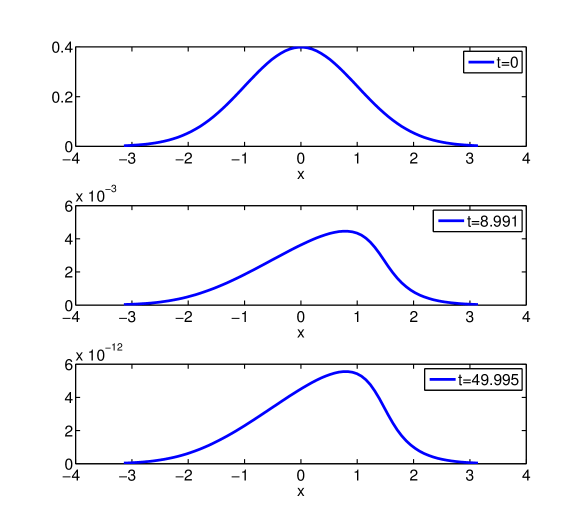
Figure 1: Damped Burger’s equation: solutions at different times

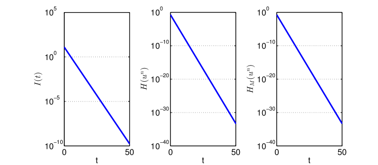
Figure 2: Damped Burger’s equation (EK): mass (left), exact Hamiltonian (middle) and modified Hamiltonian (right)

The error in the residual (15) of the linear conformal invariant (mass) is preserved exactly for EK in Figure 3 and for the LIE in Figure 4. The error in the residual of the Hamiltonian (14) is much larger in both figures, but does not show any drift as time progresses.

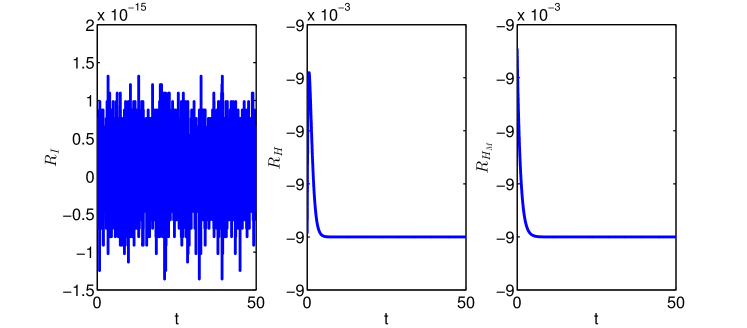
Figure 3: Damped Burger’s equation (EK): residuals of linear conformal invariant (left), exact Hamiltonian (middle) and modified Hamiltonian (right)

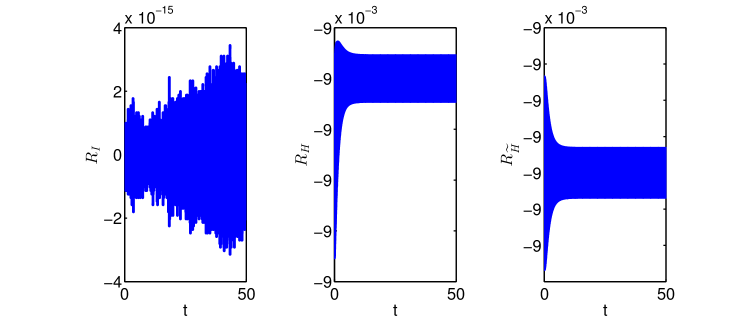
Figure 4: Damped Burger’s equation (LIE): residuals of linear conformal invariant (left), exact Hamiltonian (middle) and polarized Hamiltonian (right)

3.2 Damped Korteweg-de-Vries (KdV) equation

We consider the following damped KdV equation in [1]

$$u_{t}=\alpha(u^{2})_{x}+\rho u_{x}+\nu u_{xxx}-2\gamma u.$$

In Hamiltonian form, it reads as

$$u_{t}=\frac{\partial}{\partial x}\frac{\delta{\mathcal{H}}}{\delta u}-2\gamma u,\quad{\mathcal{H}}(u)=\int\left(\frac{\alpha}{3}u^{3}+\frac{\rho}{2}u^{2}-\frac{\nu}{2}u_{x}^{2}\right)dx.$$ (17)

The damped KdV equation was solved with the projected exponential Runge-Kutta methods in [1] and with the conformal multisymplectic method in [14]. It possesses the quadratic conformal invariant $I=\int u^{2}dx$ [1, 14].

The semi-discrete form of (17) given as

$$\dot{{\bm{u}}}=\alpha D_{1}\left({\bm{u}}\odot{\bm{u}}\right)+\rho D_{1}{\bm{u}}+\nu D_{3}{\bm{u}}-2\gamma{\bm{u}},$$

where the matrix $D_{3}=D_{1}D_{2}$ approximates the third order derivative $\partial_{xxx}$. The discrete Hamiltonian is given by

$$H({\bm{u}}^{n})=\int\left(\frac{\alpha}{3}({\bm{u}}^{n})^{3}+\frac{\rho}{2}({\bm{u}}^{n})^{2}-D_{1}\frac{\nu}{2}({\bm{u}}^{n})^{2}\right)dx.$$

The exponential integrators in Section 2, give rise to the following schemes:

• CIMP:

  $$\frac{e^{X_{1}}{\bm{u}}^{n+1}-e^{X_{0}}{\bm{u}}^{n}}{\Delta t}= \;\alpha D_{1}\frac{e^{X_{0}}{\bm{u}}^{n}\odot e^{X_{0}}{\bm{u}}^{n}+e^{X_{1}}{\bm{u}}^{n+1}\odot e^{X_{1}}{\bm{u}}^{n+1}}{2}$$

  $$+\rho D_{1}\frac{e^{X_{0}}{\bm{u}}^{n}+e^{X_{1}}{\bm{u}}^{n+1}}{2}+\nu D_{3}\frac{e^{X_{0}}{\bm{u}}^{n}+e^{X_{1}}{\bm{u}}^{n+1}}{2}$$

• EK:

  $$\frac{e^{X_{1}}{\bm{u}}^{n+1}-e^{X_{0}}{\bm{u}}^{n}}{\Delta t} = \alpha D_{1}\frac{e^{X_{0}}{\bm{u}}^{n}\odot e^{X_{1}}{\bm{u}}^{n+1}}{2}+\rho D_{1}\frac{e^{X_{0}}{\bm{u}}^{n}+e^{X_{1}}{\bm{u}}^{n+1}}{2}$$

  $$+\ \nu D_{3}\frac{e^{X_{0}}{\bm{u}}^{n}+e^{X_{1}}{\bm{u}}^{n+1}}{2}$$

  which preserves the modified Hamiltonian (9).

• LIE:

  $$\frac{e^{X_{2}}{\bm{u}}^{n+2}-e^{X_{0}}{\bm{u}}^{n}}{2\Delta t} = \frac{\alpha}{3}D_{1}\left(e^{X_{1}}{\bm{u}}^{n+1}\odot\left(e^{X_{2}}{\bm{u}}^{n+2}+e^{X_{1}}{\bm{u}}^{n+1}+e^{X_{0}}{\bm{u}}^{n}\right)\right)$$

  $$+\ \frac{\rho}{2}D_{1}(e^{X_{2}}{\bm{u}}^{n+2}+e^{X_{0}}{\bm{u}}^{n})+\frac{\nu}{2}D_{3}(e^{X_{2}}{\bm{u}}^{n+2}+e^{X_{0}}{\bm{u}}^{n})$$

  which preserves the polarized Hamiltonian

  $$\widetilde{H}({\bm{u}}^{n},{\bm{u}}^{n+1}) = \int\left(\frac{\alpha}{9}(({\bm{u}}^{n})^{2}{\bm{u}}^{n+1}+({\bm{u}}^{n+1})^{2}{\bm{u}}^{n})+\frac{\rho}{4}(({\bm{u}}^{n})^{2}+({\bm{u}}^{n+1})^{2})\right.$$

  $$\qquad\left.-D_{1}\frac{\nu}{4}(({\bm{u}}^{n})^{2}+({\bm{u}}^{n+1})^{2})\right)dx.$$

We consider the KdV equation on $[-10,10]$ ($L=10$) in [1] with the parameter values

$$\nu=-10^{-5},\quad\gamma=10^{-2},\quad\alpha=-3/8,\quad\rho=-10.$$

The mesh sizes are $\Delta x=0.0808$ and $\Delta t=0.009$ with the final time $T=50$. The initial condition is given with the Gaussian wave profile

$$u(x,0)=\frac{2e^{-2x^{2}}}{\sqrt{2\pi}}.$$

The numerical solutions develop almost a vertical front, in form a series of wave-trains in Figure 5 as in [1].

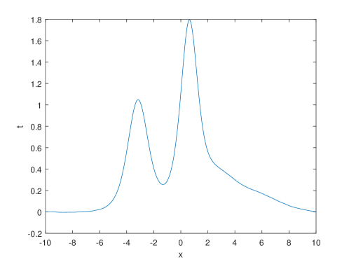
Figure 5: Solution of the damped KdV equation at final time

The EK and the LIE schemes preserve the quadratic conformal invariant with a moderate accuracy in Figures 6-7, whereas the error in the residual of the quadratic conformal invariant and modified Hamiltonian are diminishing in Figure 6 as time progresses.

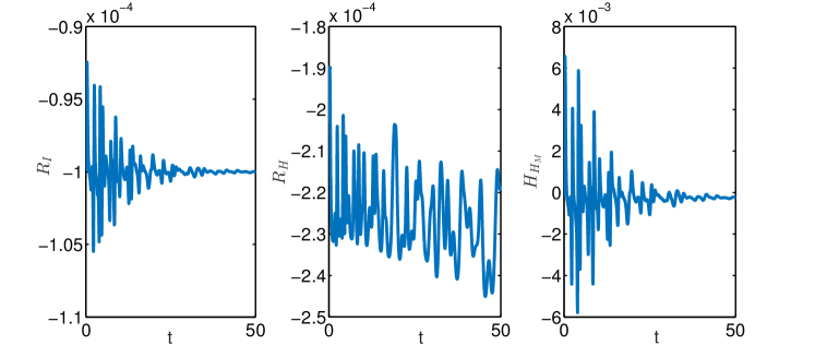
Figure 6: Damped KdV equation (EK): residuals of quadratic conformal invariant (left), exact Hamiltonian (middle) and modified Hamiltonian (right)

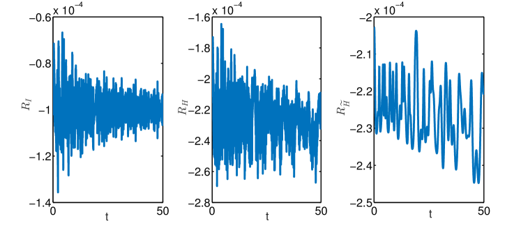
Figure 7: Damped KdV equation (LIE): residuals of quadratic conformal invariant (left), exact Hamiltonian (middle) and polarized Hamiltonian (right)

Again, the numerical results for the CIMP are similar to the EK, therefore they are not displayed.

3.3 Damped nonlinear Schrödinger (NLS) equation

We consider the following damped NLS equation [6, 13, 23, 15]

$$i\psi_{t}=-\psi_{xx}-\alpha|\psi|^{2}\psi-i\frac{\gamma}{2}\psi,$$ (18)

where $\alpha>0$ is a constant parameter, and $\gamma>0$ is a damping coefficient. The equation (18) can be written through decomposing $\psi=u+iv$ in real and imaginary components as

$$u_{t} =-v_{xx}-\alpha(u^{2}+v^{2})v-\frac{\gamma}{2}u,$$ (19)

$$v_{t} =u_{xx}+\alpha(u^{2}+v^{2})u-\frac{\gamma}{2}v.$$

The system (19) can be recast into a damped Hamiltonian system

$$\begin{pmatrix}u_{t}\\ v_{t}\end{pmatrix}=\begin{pmatrix}0&-1\\ 1&0\end{pmatrix}\begin{pmatrix}\frac{\delta{\mathcal{H}}}{\delta u}\\ \frac{\delta{\mathcal{H}}}{\delta v}\end{pmatrix}-\frac{\gamma}{2}\begin{pmatrix}u\\ v\end{pmatrix},$$

with the Hamiltonian

$$\quad{\mathcal{H}}(u,v)=\int\left(\frac{\alpha}{4}(u^{2}+v^{2})^{2}-\frac{1}{2}(u_{x}^{2}+v_{x}^{2})\right)dx.$$

Semidiscretization with finite differences gives the following ODE system

$$\dot{{\bm{u}}} =-D_{2}{\bm{v}}-\alpha\left({\bm{u}}\odot{\bm{u}}+{\bm{v}}\odot{\bm{v}}\right)\odot{\bm{v}}-\frac{\gamma}{2}{\bm{u}},$$ (20)

$$\dot{{\bm{v}}} =D_{2}{\bm{u}}+\alpha\left({\bm{u}}\odot{\bm{u}}+{\bm{v}}\odot{\bm{v}}\right)\odot{\bm{u}}-\frac{\gamma}{2}{\bm{v}},$$

with the discrete Hamiltonian

$$H({\bm{u}}^{n},{\bm{v}}^{n})=\int\left(\frac{\alpha}{4}((({\bm{u}}^{n})^{2}+({\bm{v}}^{n})^{2}))^{2}-\frac{1}{2}(D_{1}({\bm{u}}^{n})^{2}+D_{1}({\bm{u}}^{n})^{2})\right)dx.$$

The damped NLS equation (18) has two quadratic conformal invariants; the mass $I_{1}=\int(u^{2}+v^{2})dx$ and the momentum $I_{2}=\int(v_{x}u-u_{x}v)dx$. For this example, we compare the results with the implicit EAVF method and the LIE integrator.

• Applying the implicit EAVF method (10) to the ODE system (20) gives the following scheme

  $$\frac{e^{X_{1}}{\bm{u}}^{n+1}-e^{X_{0}}{\bm{u}}^{n}}{\Delta t} =-\frac{1}{2}D_{2}(e^{X_{1}}{\bm{v}}^{n+1}+e^{X_{0}}{\bm{v}}^{n})-\alpha\int_{0}^{1}\left({\bm{u}}_{\xi}^{n}\odot{\bm{u}}_{\xi}^{n}+{\bm{v}}_{\xi}^{n}\odot{\bm{v}}_{\xi}^{n}\right)\odot{\bm{v}}_{\xi}^{n}d\xi,$$

  $$\frac{e^{X_{1}}{\bm{v}}^{n+1}-e^{X_{0}}{\bm{v}}^{n}}{\Delta t} =\frac{1}{2}D_{2}(e^{X_{1}}{\bm{u}}^{n+1}+e^{X_{0}}{\bm{u}}^{n})+\alpha\int_{0}^{1}\left({\bm{u}}_{\xi}^{n}\odot{\bm{u}}_{\xi}^{n}+{\bm{v}}_{\xi}^{n}\odot{\bm{v}}_{\xi}^{n}\right)\odot{\bm{u}}_{\xi}^{n}d\xi,$$

  where

  $${\bm{u}}_{\xi}^{n}=\xi e^{X_{1}}{\bm{u}}^{n+1}+(1-\xi)e^{X_{0}}{\bm{u}}^{n},\qquad{\bm{v}}_{\xi}^{n}=\xi e^{X_{1}}{\bm{v}}^{n+1}+(1-\xi)e^{X_{0}}{\bm{v}}^{n},$$

  and

  $$\quad X_{1}=\frac{\gamma\Delta t}{4},\quad X_{0}=-\frac{\gamma\Delta t}{4}.$$

• The LIE (13) gives the scheme

  $$\frac{e^{X_{2}}{\bm{u}}^{n+2}-e^{X_{0}}{\bm{u}}^{n}}{2\Delta t} =-\frac{1}{2}D_{2}\left(e^{X_{2}}{\bm{v}}^{n+2}+e^{X_{0}}{\bm{v}}^{n}\right)$$

  $$\qquad-\frac{\alpha}{2}\left(e^{X_{1}}{\bm{u}}^{n+1}\odot e^{X_{1}}{\bm{u}}^{n+1}+e^{X_{1}}{\bm{v}}^{n+1}\odot e^{X_{1}}{\bm{v}}^{n+1}\right)\odot\left(e^{X_{2}}{\bm{v}}^{n+2}+e^{X_{0}}{\bm{v}}^{n}\right),$$

  $$\frac{e^{X_{2}}{\bm{v}}^{n+2}-e^{X_{0}}{\bm{v}}^{n}}{2\Delta t} =\frac{1}{2}D_{2}\left(e^{X_{2}}{\bm{u}}^{n+2}+e^{X_{0}}{\bm{u}}^{n}\right)$$

  $$\qquad+\frac{\alpha}{2}\left(e^{X_{1}}{\bm{u}}^{n+1}\odot e^{X_{1}}{\bm{u}}^{n+1}+e^{X_{1}}{\bm{v}}^{n+1}\odot e^{X_{1}}{\bm{v}}^{n+1}\right)\odot\left(e^{X_{2}}{\bm{u}}^{n+2}+e^{X_{0}}{\bm{u}}^{n}\right),$$

  where

  $$X_{2}=\frac{\gamma\Delta t}{2},\quad X_{1}=0,\quad X_{0}=-\frac{\gamma\Delta t}{2}.$$

  The polarized Hamiltonian is given by

  $$\widetilde{H}({\bm{u}}^{n},{\bm{u}}^{n+1}) = \int\left(\frac{\alpha}{4}(({\bm{u}}^{n})^{2}({\bm{u}}^{n+1})^{2}+({\bm{v}}^{n})^{2}({\bm{u}}^{n+1})^{2}+{\bm{u}}^{n}{\bm{v}}^{n}+{\bm{u}}^{n+1}{\bm{v}}^{n+1})\right.$$

  $$\qquad\left.-D_{1}\frac{1}{2}(({\bm{u}}^{n})^{2}+({\bm{u}}^{n+1})^{2})\right)dx.$$

For the numerical experiment, we consider the damped NLS equation [5, 15] on $[-25,25]$ with the mesh sizes $\Delta x=50/1024$ and $\Delta t=0.001$, and the target time is $T=10$. We fix the parameter $\alpha=2$, and take the initial condition as $\psi(x,0)=\text{sech}(x)e^{2ix}$.

Figure 8 shows solutions at initial and final times by using the EAVF and LIE schemes with $\gamma=5e-3$. The damped solitary wave is traveling from left to right as required, by preserving the phase space structure.

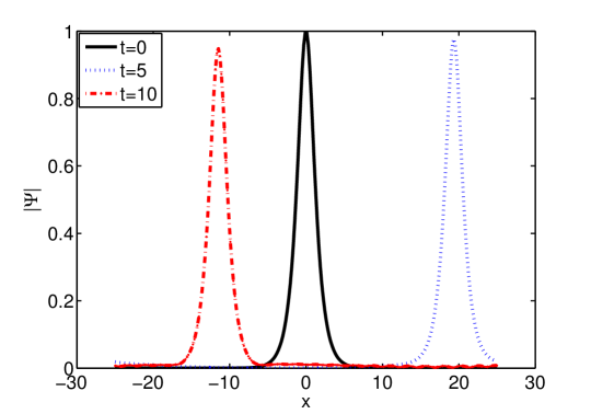
Figure 8: Solution of the damped NLS equation

In Figures 9-11, residuals of the energy balance of the quadratic conformal invariants and the Hamiltonian are plotted. The EAVF and LIE schemes do not preserve the dissipative rate of the invariants exactly, whereas the error in the residuals for LIE is lower than the EAVF. In Figure 11, errors in the residuals are smaller for small damping factors $\gamma=5e-4$ plotted than those in Figure 10, whereas the error in residual of the polarized Hamiltonian is exactly preserved.

,

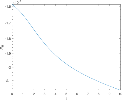
Figure 9: Damped NLS equation with $\gamma=5e-3$ (EAVF): residuals of mass (left), momentum (middle) and exact Hamiltonian (right)

,

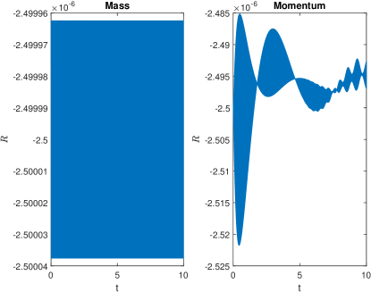
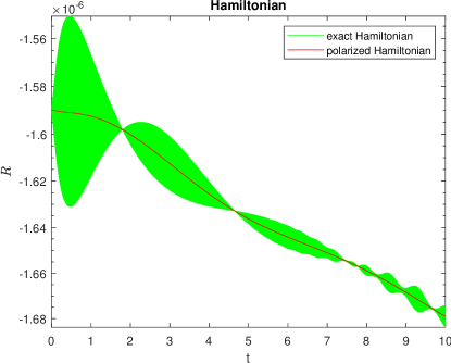
Figure 10: Damped NLS equation with $\gamma=5e-3$ (LIE): residuals of mass (left), momentum (middle) and Hamiltonians (right)

,

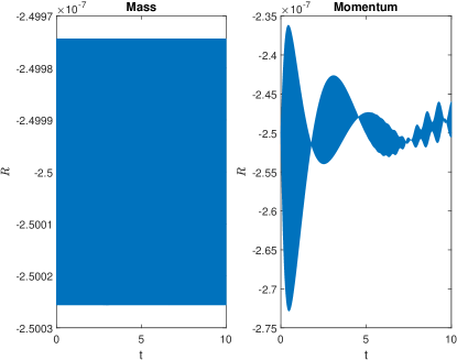
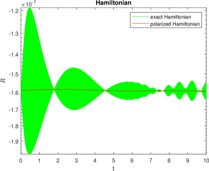
Figure 11: Damped NLS equation with $\gamma=5e-4$ (LIE): residuals of mass (left), momentum (middle) and Hamiltonians (right)

The CPU time needed for the solution of the systems with LIE is 55.1 seconds, and for the EAVF 70.4 seconds, which supports that LIE method is computationally more advantageous than the EAVF method.

4 Conclusions

Linearly implicit exponential integrators preserve linear conformal invariants exactly and preserve the quadratic invariants, cubic and quartic Hamiltonians more accurately when the damping coefficient is small. Symmetry of LIE scheme guarantees stable long-time behavior of the solutions. Compared with the fully implicit methods such as EAVF method, LIE methods show a lower computational cost as illustrated by the damped NLS equation in long-term integration. The computational advantages of the linearly implicit methods would be more significant for higher dimensional PDEs, which is the subject of future research as well as an extension to time-dependent damping.

References

• [1] A. Bhatt. Projected exponential Runge–Kutta methods for preserving dissipative properties of perturbed constrained Hamiltonian systems. Journal of Computational and Applied Mathematics, 394:113556, 2021.
• [2] A. Bhatt, D. Floyd, and B. E. Moore. Second order conformal symplectic schemes for damped Hamiltonian systems. Journal of Scientific Computing, 66(3):1234–1259, 2016.
• [3] A. Bhatt and B. E. Moore. Exponential integrators preserving local conservation laws of PDEs with time-dependent damping/driving forces. Journal of Computational and Applied Mathematics, 352:341–351, 2019.
• [4] Ashish Bhatt and Brian E. Moore. Structure-preserving exponential Runge-Kutta methods. SIAM Journal on Scientific Computing, 39(2):A593–A612, 2017.
• [5] Jiaxiang Cai and Bangyu Shen. Linearly implicit local energy-preserving algorithm for a class of multi-symplectic Hamiltonian PDEs. Computational & Applied Mathematics, 41(1):Paper No. 33, 19, 2022.
• [6] Jiaxiang Cai and Haihui Zhang. Efficient schemes for the damped nonlinear Schrödinger equation in high dimensions. Applied Mathematics Letters, 102:106158, 7, 2020.
• [7] E. Celledoni, V. Grimm, R. I. McLachlan, D. I. McLaren, D. O’Neale, B. Owren, and G. R. W. Quispel. Preserving energy resp. dissipation in numerical PDEs using the ”average vector field” method. Journal of Computational Physics, 231(20):6770–6789, 2012.
• [8] E. Celledoni, R. I. McLachlan, B. Owren, and G. R. W. Quispel. Geometric properties of Kahan’s method. Journal of Physics. A. Mathematical and Theoretical, 46(2):025201, 12, 2013.
• [9] D. Cohen and E. Hairer. Linear energy-preserving integrators for Poisson systems. BIT. Numerical Mathematics, 51(1):91–101, 2011.
• [10] M. Dahlby and B. Owren. A general framework for deriving integral preserving numerical methods for PDEs. SIAM Journal on Scientific Computing, 33(5):2318–2340, 2011.
• [11] Sø lve Eidnes and Lu Li. Linearly implicit local and global energy-preserving methods for PDEs with a cubic Hamiltonian. SIAM Journal on Scientific Computing, 42(5):A2865–A2888, 2020.
• [12] Sø lve Eidnes, Lu Li, and Shun Sato. Linearly implicit structure-preserving schemes for Hamiltonian systems. Journal of Computational and Applied Mathematics, 387:Paper No. 112489, 12, 2021.
• [13] Hao Fu, Wei-En Zhou, Xu Qian, Song-He Song, and Li-Ying Zhang. Conformal structure-preserving method for damped nonlinear Schrödinger equation. Chinese Physics B, 25(11):110201, 2016.
• [14] Feng Guo. Second order conformal multi-symplectic method for the damped Korteweg–de Vries equation*. Chinese Physics B, 28(5):050201, 2019.
• [15] Chaolong Jiang, Wenjun Cai, and Yushun Wang. Optimal error estimate of a conformal fourier pseudo-spectral method for the damped nonlinear Schrödinger equation. Numerical Methods for Partial Differential Equations, 34(4):1422–1454, 2018.
• [16] W. Kahan. Unconventional numerical methods for trajectory calculations. Technical report, Computer Science Division and Department of Mathematics, University of California, Berkeley, 1993. Unpublished lecture notes.
• [17] W. Kahan and Ren-Chang Li. Unconventional schemes for a class of ordinary differential equations with applications to the Korteweg-de Vries equation. Journal of Computational Physics, 134(2):316 – 331, 1997.
• [18] Lu Li. A new symmetric linearly implicit exponential integrator preserving polynomial invariants or Lyapunov functions for conservative or dissipative systems. Journal of Computational Physics, 449:Paper No. 110800, 13, 2022.
• [19] R. I. McLachlan and G. R. W. Quispel. Splitting methods. Acta Numerica, 11:341–434, 2002.
• [20] B. E. Moore. Multi-conformal-symplectic PDEs and discretizations. Journal of Computational and Applied Mathematics, 323:1–15, 2017.
• [21] B. E. Moore. Exponential integrators based on discrete gradients for linearly damped/driven Poisson systems. Journal of Scientific Computing, 87(2):Paper No. 56, 18, 2021.
• [22] Brian E. Moore. Conformal multi-symplectic integration methods for forced-damped semi-linear wave equations. Mathematics and Computers in Simulation, 80(1):20–28, 2009.
• [23] Brian E. Moore, Laura Noreña, and Constance M. Schober. Conformal conservation laws and geometric integration for damped Hamiltonian PDEs. Journal of Computational Physics, 232(1):214–233, 2013.
• [24] G. R. W. Quispel and D. I. McLaren. A new class of energy-preserving numerical integration methods. Journal of Physics. A. Mathematical and Theoretical, 41(4):045206, 7, 2008.
• [25] M. Uzunca and B. Karasözen. Linearly implicit methods for Allen-Cahn equation. Applied Mathematics and Computation, 450:Paper No. 127984, 11, 2023.