Sparse grid based Chebyshev HOPGD for parameterized linear systems

Abstract

We consider approximating solutions to parameterized linear systems of the form $A(\mu_{1},\mu_{2})x(\mu_{1},\mu_{2})=b$, where $(\mu_{1},\mu_{2})\in\mathbb{R}^{2}$. Here the matrix $A(\mu_{1},\mu_{2})\in\mathbb{R}^{n\times n}$ is nonsingular, large, and sparse and depends nonlinearly on the parameters $\mu_{1}$ and $\mu_{2}$. Specifically, the system arises from a discretization of a partial differential equation and $x(\mu_{1},\mu_{2})\in\mathbb{R}^{n}$, $b\in\mathbb{R}^{n}$. This work combines companion linearization with the Krylov subspace method preconditioned bi-conjugate gradient (BiCG) and a decomposition of a tensor matrix of precomputed solutions, called snapshots. As a result, a reduced order model of $x(\mu_{1},\mu_{2})$ is constructed, and this model can be evaluated in a cheap way for many values of the parameters. The decomposition is performed efficiently using the sparse grid based higher-order proper generalized decomposition (HOPGD) presented in [Lu, Blal, and Gravouil, Internat. J. Numer. Methods Engrg., 114:1438–1461, 2018], and the snapshots are generated as one variable functions of $\mu_{1}$ or of $\mu_{2}$, as proposed in [Correnty, Jarlebring, and Szyld, Preprint on arXiv, 2022 https://arxiv.org/abs/2212.04295]. Tensor decompositions performed on a set of snapshots can fail to reach a certain level of accuracy, and it is not possible to know a priori if the decomposition will be successful. This method offers a way to generate a new set of solutions on the same parameter space at little additional cost. An interpolation of the model is used to produce approximations on the entire parameter space, and this method can be used to solve a parameter estimation problem. Numerical examples of a parameterized Helmholtz equation show the competitiveness of our approach. The simulations are reproducible, and the software is available online.

1 Introduction

We are interested in approximating solutions to linear systems of the form

(1) $$A(\mu_{1},\mu_{2})x(\mu_{1},\mu_{2})=b,$$

for many different values of the parameters $\mu_{1},\mu_{2}$. Here $A(\mu_{1},\mu_{2})\in\mathbb{R}^{n\times n}$ is a large and sparse nonsingular matrix with a nonlinear dependence on $\mu_{1}\in[a_{1},b_{1}]\subset\mathbb{R}$ and $\mu_{2}\in[a_{2},b_{2}]\subset\mathbb{R}$ and $x(\mu_{1},\mu_{2})\in\mathbb{R}^{n}$, $b\in\mathbb{R}^{n}$. This work combines companion linearization, a technique from the study of nonlinear eigenvalue problems, with the Krylov subspace method bi-conjugate gradient (BiCG) [21, 33] and a tensor decomposition to construct a reduced order model. This smaller model can be evaluated in an inexpensive way to approximate the solution to (1) for many values of the parameters. Additionally, the model can be used to solve a parameter estimation problem, i.e., to simultaneously estimate $\mu_{1}$ and $\mu_{2}$ for a given solution vector where these parameters are not known.

Specifically, our proposed method is based on a decomposition of a tensor matrix of precomputed solutions to (1), called snapshots, where the systems arise from discretizations of parameterized partial differential equations (PDEs). In this way, building the reduced order model can be divided into two main parts:

1. Generate the snapshots.

2. Perform the tensor decomposition.

We assume further that the system matrix can be expressed as the sum of products of matrices and functions, i.e.,

(2) $$A(\mu_{1},\mu_{2})=C_{1}f_{1}(\mu_{1},\mu_{2})+\cdots+C_{n_{f}}f_{n_{f}}(\mu_{1},\mu_{2}),$$

where $n_{f}\ll n$ and $f_{1},\ldots,f_{n_{f}}$ are nonlinear scalar functions in the parameters $\mu_{1}$ and $\mu_{2}$.

Previously proposed methods of this variety, e.g., [9, 10, 35, 36, 37, 38], generate the snapshots in an offline stage, and, thus, a linear system of dimension $n\times n$ must be solved for each pair $(\mu_{1},\mu_{2})$ in the tensor matrix. Here we instead compute the snapshots with the method proposed in [17], Preconditioned Chebyshev BiCG for parameterized linear systems. This choice allows for greater flexibility in the selection of the set of snapshots included in the tensor, as the approximations are generated as one variable functions of $\mu_{1}$ or of $\mu_{2}$, i.e., with one parameter frozen. These functions are cheap to evaluate for different values of the parameter, and this method is described in Section 2.

The tensor matrix of precomputed snapshots has a particular structure, as we consider sparse grid sampling in the parameter space. This is a way to overcome the so-called curse of dimensionality since the number of snapshots to generate and store grows exponentially with the dimension when the sampling is performed on a conventional full grid. The decomposition is performed with a variant of the higher-order proper generalized decomposition (HOPGD), as proposed in [35]. The method HOPGD [38] decomposes a tensor of snapshots sampled on a full grid. The approach here has been adapted for this particular setting with fewer snapshots and, as in the standard implementation, results in a separated expression in $\mu_{1}$ and $\mu_{2}$. Once constructed, the decomposition is interpolated to approximate solutions to (1) corresponding to all parameters $(\mu_{1},\mu_{2})\in[a_{1},b_{1}]\times[a_{2},b_{2}]$.

More precisely, an alternating directions, greedy algorithm is used to perform the decomposition, where the cost of each step of the method grows linearly with the number of unknowns $n$. The basis vectors for the decomposition are not known beforehand, similar to the established proper generalized decomposition (PGD), often used to create reduced order models of PDEs which are separated in the time and space variables. The method PGD has been used widely in the study of highly nonlinear PDEs [13, 14, 15] and has been generalized to solve multiparametric problems; see, for instance, [5, 6].

As performing the decomposition can be done efficiently, generating the snapshots is the dominating cost of building the reduced order model. In general, we cannot guarantee that the error in a tensor decomposition for a certain set of snapshots will reach a specified accuracy level. Additionally, it is not possible to know a priori which sets of snapshots will lead to a successful decomposition, even with modest standards for the convergence [30]. In the case of the decomposition failing to converge for a given tensor, our proposed method offers an efficient way to generate a new set of snapshots on the same parameter space $[a_{1},b_{1}]\times[a_{2},b_{2}]$ with little extra computation. These snapshots can be used to construct a new reduced order model for the same parameter space in an identical, efficient way. This is the main contribution developed in this work.

Evaluating the resulting reduced order model is in general much more efficient than solving the systems individually for each choice of the parameters [35]. Reliable and accurate approximations are available for a variety of parameter choices, and parameter estimation can be performed in a similarly competitive way. Details regarding the construction of the reduced order model are found in Section 3, and numerical simulations of a parameterized Helmholtz equation and a parameterized advection-diffusion equation are presented in Sections 4 and 5, respectively. All experiments were carried out on a 2.3 GHz Dual-Core Intel Core i5 processor with 16 GB RAM, and the corresponding software can be found online.

2 Generating snapshots with Preconditioned Chebyshev BiCG

Constructing an accurate reduced order model of $x(\mu_{1},\mu_{2})$ requires sampling of solutions to (1) for many different values of the parameters $\mu_{1}$ and $\mu_{2}$. Parameterized linear systems have been studied in several prior works, for example, in the context of Tikhonov regularization for ill-posed problems [25, 29], as well as in [32], where the solutions were approximated by low-rank tensors, and in [44] with parameterized right-hand sides. Additionally, approaches based on companion linearization were proposed in [26], as well as in [16, 28] with a linearization based on an infinite Taylor series expansion.

Reduced order models based on sampling of snapshot solutions are typically constructed from finite element approximations, generated in an offline stage at a significant computational cost. We base our approach to obtain the snapshot solutions on an adapted version of the method Preconditioned Chebyshev BiCG for parameterized linear systems, originally proposed in [17]. Here the unique solution to a companion linearization, formed from a Chebyshev approximation using Chebfun [18], is generated in a preconditioned BiCG [21, 33] setting. Two executions of this method generate all solutions corresponding to the values of the parameters shown in Figure 2. Specifically, one execution for all solutions on the line $\mu_{1}=\mu_{1}^{*}$ and one execution for all solutions on the line $\mu_{2}=\mu_{2}^{*}$ in the plane $[a_{1}\times b_{1}]\times[a_{2}\times b_{2}]$. In this way, we generate solutions fixed in one parameter. Moreover, the sampling represented here is sufficient to build a reliable reduced order model with the strategy presented in [35]. We summarize the method Preconditioned Chebyshev BiCG, for the sake of self-containment, as follows.

A Chebyshev approximation of $A(\mu_{1},\mu_{2})$ for a fixed $\mu_{2}^{*}\in\mathbb{R}$ is given by $\hat{P}(\mu_{1})$, where

(3) $$A(\mu_{1},\mu_{2}^{*})\approx\hat{P}(\mu_{1})\coloneqq\hat{P}_{0}\hat{\tau}_{0}(\mu_{1})+\ldots+\hat{P}_{d_{1}}\hat{\tau}_{d_{1}}(\mu_{1})$$

and, for a fixed $\mu_{1}^{*}\in\mathbb{R}$, by $\tilde{P}(\mu_{2})$, i.e.,

(4) $$A(\mu_{1}^{*},\mu_{2})\approx\tilde{P}(\mu_{2})\coloneqq\tilde{P}_{0}\tilde{\tau}_{0}(\mu_{2})+\ldots+\tilde{P}_{d_{2}}\tilde{\tau}_{d_{2}}(\mu_{2}).$$

Here $\hat{\tau}_{\ell}$ is the degree $\ell$ Chebyshev polynomial on $[-c_{1},c_{1}]$, $\tilde{\tau}_{\ell}$ is the degree $\ell$ Chebyshev polynomial on $[-c_{2},c_{2}]$, and $\hat{P}_{\ell}$, $\tilde{P}_{\ell}\in\mathbb{R}^{n\times n}$ are the corresponding interpolation coefficients. These coefficients are computed efficiently by a discrete cosine transform of the one variable scalar functions

(5) $$f_{k}(\mu_{1},\mu_{2}^{*})\eqqcolon\hat{f}_{k}(\mu_{1}),\qquad f_{k}(\mu_{1}^{*},\mu_{2})\eqqcolon\tilde{f}_{k}(\mu_{2}),\qquad k=1,\ldots,n_{f},$$

in (2). Note, $c_{l}\in\mathbb{R}$ is chosen such that $[a_{l},b_{l}]\subseteq[-c_{l},c_{l}]$, for $l=1,2$. A companion linearization based on the linear system

(6) $$\hat{P}(\mu_{1})\hat{x}(\mu_{1})=b$$

with $\hat{x}(\mu_{1})=\hat{x}(\mu_{1},\mu_{2}^{*})\approx x(\mu_{1},\mu_{2}^{*})$, where $x(\mu_{1},\mu_{2}^{*})$ is as in (1), and a fixed $\mu_{2}^{*}$ is given by

$$\left(\begin{bmatrix}0&I&&&&&\\ I&0&I&&&&\\ &I&0&I&&&\\ &&&\ddots&&&\\ &&&&I&0&I\\ \hat{P}_{0}&\hat{P}_{1}&\cdots&\cdots&\hat{P}_{d_{1}-3}&(-\hat{P}_{d_{1}}+\hat{P}_{d_{1}-2})&\hat{P}_{d_{1}-1}\end{bmatrix}-\frac{\mu_{1}}{c_{1}}\begin{bmatrix}I&&&&&\\ &2I&&&&\\ &&2I&&&\\ &&&\ddots&&\\ &&&&2I&\\ &&&&&-2\hat{P}_{d_{1}}\\ \end{bmatrix}\right)\begin{bmatrix}u_{0}(\mu_{1})\\ u_{1}(\mu_{1})\\ u_{2}(\mu_{1})\\ \vdots\\ u_{d_{1}-2}(\mu_{1})\\ u_{d_{1}-1}(\mu_{1})\end{bmatrix}=\begin{bmatrix}0\\ 0\\ 0\\ \vdots\\ 0\\ b\end{bmatrix}$$

with $u_{\ell}(\mu_{1})\coloneqq\hat{\tau}_{\ell}(\mu_{1})\hat{x}(\mu_{1},\mu_{2}^{*})$, for $\ell=0,\ldots,d_{1}-1$. The linearization has the form

(7) $$\left(\hat{K}-\mu_{1}\hat{M}\right)u(\mu_{1})=c,$$

where $\hat{K},\hat{M}\in\mathbb{R}^{d_{1}n\times d_{1}n}$ are coefficient matrices, independent of the parameter $\mu_{1}$, $c\in\mathbb{R}^{d_{1}n}$ is a constant vector, and the solution $u(\mu_{1})$ is unique. This linearization, inspired by the work [19] and studied fully in [17], relies on the well-known three-term recurrence of the Chebyshev polynomials:

(8) $$\hat{\tau}_{0}(\mu_{1})\coloneqq 1,\quad\hat{\tau}_{1}(\mu_{1})\coloneqq\frac{1}{c_{1}}\mu_{1},\quad\hat{\tau}_{\ell+1}(\mu_{1})\coloneqq\frac{2}{c_{1}}\mu_{1}\hat{\tau}_{\ell}(\mu_{1})-\hat{\tau}_{\ell-1}(\mu_{1}).$$

Solutions to the systems in (7) for many different $\mu_{1}$ are approximated with the Krylov subspace method bi-conjugate gradient for shifted systems [2, 23]. Specifically, we approximate an equivalent right preconditioned system, where the system matrix incorporates a shift with the identity matrix. This system is given by

(9a) $$(\hat{K}-\mu_{1}\hat{M})(\hat{K}-\hat{\sigma}\hat{M})^{-1}\hat{u}(\mu_{1})=c$$

(9b) $$\iff (\hat{K}-\mu_{1}\hat{M}+\hat{\sigma}\hat{M}-\hat{\sigma}\hat{M})(\hat{K}-\hat{\sigma}\hat{M})^{-1}\hat{u}(\mu_{1})=c$$

(9c) $$\iff \left(I+(-\mu_{1}+\hat{\sigma})\hat{M}(\hat{K}-\hat{\sigma}\hat{M})^{-1}\right)\hat{u}(\mu_{1})=c$$

with $\hat{u}(\mu_{1})=(\hat{K}-\hat{\sigma}\hat{M})u(\mu_{1})$. The $k$th approximation comes from the Krylov subspace generated from the matrix $\hat{M}(\hat{K}-\hat{\sigma}\hat{M})^{-1}$ and the vector $c$, defined by

(10) $$\mathcal{K}_{k}\coloneqq\text{span}\{c,\hat{M}(\hat{K}-\hat{\sigma}\hat{M})^{-1}c,\ldots,(\hat{M}(\hat{K}-\hat{\sigma}\hat{M})^{-1})^{k-1}c\}.$$

Here the shift- and scaling- invariance properties of Krylov subspaces have been exploited, i.e., $\mathcal{K}_{k}=\tilde{\mathcal{K}}_{k}$, where $\tilde{\mathcal{K}}_{k}$ is the Krylov subspace generated from the matrix $(I+(-\mu_{1}+\hat{\sigma})\hat{M}(\hat{K}-\hat{\sigma}\hat{M})^{-1})$ and the vector $c$. Note, several Krylov methods have been developed specifically to approximate shifted systems of the form (9c). See, for example, [22, 24, 42, 45], as well as in [7, 8], where shift-and-invert preconditioners were considered.

As we consider a BiCG setting, we require also a basis matrix for the subspace defined by

(11) $$\mathcal{L}_{k}\coloneqq\text{span}\{\tilde{c},\left(\hat{M}(\hat{K}-\hat{\sigma}\hat{M})^{-1}\right)^{T}\tilde{c},\ldots,\left((\hat{M}(\hat{K}-\hat{\sigma}\hat{M})^{-1})^{T}\right)^{k-1}\tilde{c}\},$$

where $\tilde{c}\in\mathbb{R}^{d_{1}n}$ and $c^{T}\tilde{c}\neq 0$. In this way, a basis matrix for the Krylov subspace (10) and a second basis matrix for the subspace (11) are built once and reused for the computation of solutions to (9) for all $\mu_{1}$ of interest. More concretely, a Lanczos biorthogonalization process generates the matrices $V_{k}$, $W_{k}\in\mathbb{R}^{d_{1}n\times k}$, $T_{k} \in\mathbb{R}^{k\times k}$, and $\underline{$T$}_{k}$, $\bar{T}^{T}_{k}\in\mathbb{R}^{(k+1)\times k}$ such that the relations

(12a) $$\hat{M}(\hat{K}-\hat{\sigma}\hat{M})^{-1}V_{k} =V_{k} T_{k} +\beta_{k}v_{k+1}e_{k}^{T} =V_{k+1} \underline{$T$}_{k},$$

(12b) $$\big{(}\hat{M}(\hat{K}-\hat{\sigma}\hat{M})^{-1}\big{)}^{T}W_{k} =W_{k} T_{k}^{T} +\gamma_{k}w_{k+1}e_{k}^{T} =W_{k+1} \bar{T}^{T}_{k}$$

hold. The columns of $V_{k}$ span the subspace (10), the columns of $W_{k}$ span the subspace (11), and the biorthogonalization procedure gives $W_{k}^{T}V_{k}=I_{k}$, where $I_{k}\in\mathbb{R}^{k\times k}$ is the identity matrix of dimension $k\times k$. Here $e_{k}$ in (12) denotes the $k$th column of $I_{k}$ and the matrices in (12) are generated independently of the parameter $\mu_{1}$. The square matrix $T_{k}$ is of the form

(13) $$T_{k}\coloneqq\begin{bmatrix}\alpha_{1}&\gamma_{1}&&&\\ \beta_{1}&\ddots&&&\\ &\ddots&&&\gamma_{k-1}\\ \ &&&\beta_{k-1}&\alpha_{k}\\ \end{bmatrix}\in\mathbb{R}^{k\times k},$$

and the tridiagonal rectangular Hessenberg matrices $\underline{T}_{k}$ and $\bar{T}^{T}_{k}$ are given by

(14) $$\underline{T}_{k}\coloneqq\begin{bmatrix}\alpha_{1}&\gamma_{1}&&\\ \beta_{1}&\ddots&\ddots&\\ &\ddots&\ddots&\gamma_{k-1}\\ \ &&\beta_{k-1}&\alpha_{k}\\ &&&\beta_{k}\end{bmatrix},\quad\bar{T}^{T}_{k}\coloneqq\begin{bmatrix}\alpha_{1}&\beta_{1}&&\\ \gamma_{1}&\ddots&\ddots&\\ &\ddots&\ddots&\beta_{k-1}\\ &&\gamma_{k-1}&\alpha_{k}\\ &&&\gamma_{k}\end{bmatrix},$$

where only the $k\times k$ principal submatrices of $\underline{T}_{k}$ and $\bar{T}^{T}_{k}$ are the transpose of each other. The Lanczos biorthogonalization process has the advantage of the so-called short-term recurrence of the Krylov basis vectors, i.e., that the matrices $\underline{T}_{k}$ and $\bar{T}^{T}_{k}$ in (12) are tridiagonal. In this way, the basis vectors are computed recursively at each iteration of the algorithm, and no additional orthogonalization procedure is required.

The same shift-and-invert preconditioner and its adjoint must be applied at each iteration of the Lanczos biorthogonalization algorithm. We consider an efficient application, derived in [4] and adapted in [31], via a block LU decomposition of the matrix $L_{\hat{\sigma}}U_{\hat{\sigma}}=(\hat{K}-\hat{\sigma}\hat{M})\Pi$, where $\Pi\coloneqq\footnotesize\begin{bmatrix}&I_{n}\\ I_{(d_{1}-1)n}\end{bmatrix}\in\mathbb{R}^{d_{1}n\times d_{1}n}$ is a permutation matrix,

$$L_{\hat{\sigma}}\coloneqq\begin{bmatrix}I&&&&&\\ -\frac{2\hat{\sigma}}{c_{1}}I&I&&&&\\ I&-\frac{2\hat{\sigma}}{c_{1}}I&I&&&\\ &&\ddots&&&\\ &&I&-\frac{2\hat{\sigma}}{c_{1}}I&I&\\ \hat{P}_{1}&\cdots&\hat{P}_{d_{1}-3}&(-\hat{P}_{d_{1}}+\hat{P}_{d_{1}+2})&(\hat{P}_{d_{1}-1}+\frac{2\hat{\sigma}}{c_{1}}\hat{P}_{d_{1}})&\hat{P}(\hat{\sigma})\\ \end{bmatrix}\in\mathbb{R}^{d_{1}n\times d_{1}n},$$

and

$$U_{\hat{\sigma}}\coloneqq\begin{bmatrix}I&&&&&-\hat{\tau}_{1}(\hat{\sigma})I\\ &I&&&&-\hat{\tau}_{2}(\hat{\sigma})I\\ &&I&&&-\hat{\tau}_{3}(\hat{\sigma})I\\ &&&\ddots&&\vdots\\ &&&&I&-\hat{\tau}_{d_{1}-1}(\hat{\sigma})I\\ &&&&&I\\ \end{bmatrix}\in\mathbb{R}^{d_{1}n\times d_{1}n}.$$

Specifically, the action of the preconditioner $(\hat{K}-\hat{\sigma}\hat{M})^{-1}$ to a vector $y\in\mathbb{R}^{d_{1}n}$ is given by

(15) $$(\hat{K}-\hat{\sigma}\hat{M})^{-1}y=\Pi U_{\hat{\sigma}}^{-1}L_{\hat{\sigma}}^{-1}y,$$

and the adjoint preconditioner is applied analogously, i.e.,

(16) $$(\hat{K}-\hat{\sigma}\hat{M})^{-T}y=L_{\hat{\sigma}}^{-T}U_{\hat{\sigma}}^{-T}\Pi^{T}y.$$

The matrix $U_{\hat{\sigma}}^{-1}$ is identical to $U_{\hat{\sigma}}$, except for a sign change in the first $d_{1}-1$ blocks in the last block column. Applying $L_{\hat{\sigma}}^{-1}$ to a vector amounts to recursively computing the first $d_{1}-1$ block elements and performing one linear solve with system matrix $\hat{P}(\hat{\sigma})\in\mathbb{R}^{n\times n}$, analogous to solving a block lower triangular system with Gaussian elimination. This linear solve can be achieved, for example, by computing one LU decomposition of $\hat{P}(\hat{\sigma})$. Note, an LU decomposition of $\hat{P}(\hat{\sigma})$ can be reused in the application of $L_{\hat{\sigma}}^{-T}$.

After the Krylov subspace basis matrices of a desired dimension $k$ have been constructed, approximations to (7) and, equivalently, approximations to (1), can be calculated efficiently for many values of the parameter $\mu_{1}$. In particular, we reuse the matrices $V_{k}$ and $T_{k}$ in (12) for the computation of each approximation to $x(\mu_{1}^{i},\mu_{2}^{*})_{i=1}^{n_{1}}$ of interest. This requires the calculations

(17a) $$y_{k}(\mu_{1}^{i}) = \left(I_{k}+(-\mu_{1}^{i}+\hat{\sigma}T_{k})\right)^{-1}(\beta e_{1}),$$

(17b) $$z_{k}(\mu_{1}^{i}) = V_{k}y_{k}(\mu_{1}^{i}),$$

(17c) $$x_{k}(\mu_{1}^{i},\mu_{2}^{*}) = \left((\hat{K}-\hat{\sigma}\hat{M})^{-1}z_{k}(\mu_{1}^{i})\right)_{1:n},$$

for $i=1,\ldots,n_{1}$. Here $\beta\coloneqq\left\lVert b\right\rVert$, where $b$ is as in (1), and $x_{k}(\mu_{1},\mu_{2}^{*})$ denotes the approximation to (1) from the Krylov subspace (10) of dimension $k$ corresponding to $(\mu_{1},\mu_{2}^{*})$. Equivalently, $x_{k}(\mu_{1},\mu_{2}^{*})\approx\hat{x}(\mu_{1},\mu_{2}^{*})$, where $\hat{x}(\mu_{1},\mu_{2}^{*})$ is the solution to the system (6). Note, the subscript on the right-hand side of (17c) denotes the first $n$ elements in the vector, and the preconditioner in (17c) is applied as in (15). Since $k\ll n$, solving the tridiagonal system in (17a) is not computationally demanding. Thus, once we build a sufficiently large Krylov subspace via one execution of the main algorithm, we have access to approximations $x_{k}(\mu_{1}^{i},\mu_{2}^{*})$ for all $\mu_{1}^{i}$ in the interval $[a_{1},b_{1}]$.

The process of approximating (1) for a fixed $\mu_{1}^{*}$ and $\mu_{2}^{j}$, for $j=1,\ldots,n_{2}$, is completely analogous to the above procedure and, thus, we provide just a summary here. A companion linearization is formed for a fixed $\mu_{1}^{*}$, which is solved to approximate $x(\mu_{1}^{*},\mu_{2}^{j})$, where $\mu_{2}^{j}\in[a_{2},b_{2}]$, for $j=1,\ldots,n_{2}$. This linearization has the form

(18) $$\left(\tilde{K}-\mu_{2}\tilde{M}\right)u(\mu_{2})=c$$

and is based on the Chebyshev approximation

(19) $$\tilde{P}(\mu_{2})\tilde{x}(\mu_{2})=b.$$

Here $\tilde{P}(\mu_{2})$ is as in (4) and $\tilde{x}(\mu_{2})=\tilde{x}(\mu_{1}^{*},\mu_{2})\approx x(\mu_{1}^{*},\mu_{2})$, where $x(\mu_{1}^{*},\mu_{2})$ is as in (1). The linearization (18) is based on a three-term recurrence as in (8), and we consider a shift-and-invert preconditioner of the form $(\tilde{K}-\tilde{\sigma}\tilde{M})^{-1}$. As in (15) and (16), the application of this particular preconditioner and its adjoint each require the solution to a linear system with matrices $\tilde{P}(\tilde{\sigma})$ and $\tilde{P}(\tilde{\sigma})^{T}$, respectively, and this must be done at each iteration of the Lanczos biorthogonalization. Analogous computations to (17) must be performed for each $\mu_{2}^{j}$ of interest. Thus, using a second application of the method Preconditioned Chebyshev BiCG for parameterized linear systems to solve (19), we have access to approximations $x_{k}(\mu_{1}^{*},\mu_{2}^{j})$ for all $\mu_{2}^{j}$ on the interval $[a_{2},b_{2}]$, obtained in a similarly efficient way.

Remark 1 (Choice of target parameter).

The use of shift-and-invert preconditioners with well-chosen $\hat{\sigma}$ ($\tilde{\sigma}$) generally result in fast convergence, i.e., a few iterations of the shifted BiCG algorithm. This is because $(\hat{K}-\mu_{1}\hat{M})(\hat{K}-\hat{\sigma}\hat{M})^{-1}\approx I$, for $\mu_{1}\approx\hat{\sigma}$ (and similarly $(\tilde{K}-\mu_{2}\tilde{M})(\tilde{K}-\tilde{\sigma}\tilde{M})^{-1}\approx I$, for $\mu_{2}\approx\tilde{\sigma}$). The result of this is that, typically, only a few matrix-vector products and linear (triangular) solves of dimension $n\times n$ are required before the algorithm terminates. Thus, we have accurate approximations to $x(\mu_{1}^{i},\mu_{2}^{*})$, $i=1,\ldots,n_{1}$ (and $x(\mu_{1}^{*},\mu_{2}^{j})$, $j=1,\ldots,n_{2}$), obtained in a cheap way. We refer to $\hat{\sigma}$ and $\tilde{\sigma}$ as target parameters for this reason.

Remark 2 (Inexact application of the preconditioner).

The LU decomposition of the matrices $\hat{P}(\hat{\sigma})$ and $\tilde{P}(\tilde{\sigma})$ of dimension $n\times n$ can be avoided entirely by considering the inexact version of Preconditioned Chebyshev BiCG for parameterized linear systems, derived and fully analyzed in [17]. This method applies the preconditioner and its adjoint approximately via iterative methods and is suitable for systems where the dimension $n$ is very large. In practice, the corresponding systems can be solved with a large amount of error once the relative residual of the outer method is sufficiently low.

Remark 3 (Structure of the companion linearization).

Though we are interested in the solution to systems which depend on two parameters, we consider an interpolation in one variable. Interpolations of functions in two variables have been studied. However, the error of the approximation outside of the interpolation nodes tends to be too large for our purposes. Additionally, the recursion in (8) is essential for the structure of the companion linearizations (7) and, analogously, in (18). In particular, solutions to (1) must only appear in the solution vector, and the matrices $\hat{K}$, $\hat{M}$ ($\tilde{K}$, $\tilde{M}$) and right-hand side vector $c$ must be constant with respect to the parameters $\mu_{1}$ and $\mu_{2}$.

Remark 4 (Error introduced by the Chebyshev approximation).

This work utilizes Chebfun [18], which computes approximations to the true Chebyshev coefficients. In particular, convergence is achieved as the approximate coefficients decay to zero, and only coefficients greater in magnitude than $10^{-16}$ are used in the approximation. In the examples which follow, we consider only twice continuously differentiable functions for $\hat{f}_{k}$ and $\tilde{f}_{k}$ in (5). Thus, the error introduced by a Chebyshev approximation is very small.

3 Sparse grid based HOPGD

Let $X(\mu_{1},\mu_{2})\in\mathbb{R}^{n\times n_{1}\times n_{2}}$ be a sparse three-dimensional matrix of precomputed snapshots. These approximations to (1), generated by two executions of the preconditioned Krylov subspace method described in Section 2, correspond to the pairs of parameters $(\mu_{1}^{i},\mu_{2}^{*})$, $i=1,\ldots,n_{1}$, and $(\mu_{1}^{*},\mu_{2}^{j})$, $j=1,\ldots,n_{2}$. Here $\mu_{1}^{i}$ are in the interval $[a_{1},b_{1}]$, $\mu_{2}^{j}$ are in the interval $[a_{2},b_{2}]$, and $\mu_{1}^{*}\in[a_{1},b_{1}]$, $\mu_{2}^{*}\in[a_{2},b_{2}]$ are fixed values. More precisely,

(20a) $$X(\mu_{1}^{i},\mu_{2}^{*}) =\hat{x}(\mu_{1}^{i},\mu_{2}^{*})\in\mathbb{R}^{n},\quad i =1,\ldots,n_{1},$$

(20b) $$X(\mu_{1}^{*},\mu_{2}^{j}) =\tilde{x}(\mu_{1}^{*},\mu_{2}^{j})\in\mathbb{R}^{n},\quad j =1,\ldots,n_{2},$$

and the remaining entries of $X(\mu_{1},\mu_{2})$ are zeros; see Figure 1 for a visualization of a tensor of this form. Note, $\hat{x}(\mu_{1}^{i},\mu_{2}^{*})=\hat{x}(\mu_{1}^{i})$ are approximations to the linear systems described in (6) and $\tilde{x}(\mu_{1}^{*},\mu_{2}^{j})=\tilde{x}(\mu_{2}^{j})$ are approximations to the systems in (19). We refer to the set

(21) $$\bm{\mu}\coloneqq(\mu_{1}^{i},\mu_{2}^{*})\cup(\mu_{1}^{*},\mu_{2}^{j}),$$

for $i=1,\ldots,n_{1}$, $j=1,\ldots,n_{2}$, as the nodes and $\bm{\mu}\subset[a_{1},b_{1}]\times[a_{2},b_{2}]$. The set of nodes corresponding to the tensor matrix $X(\mu_{1},\mu_{2})$ in Figure 1 are visualized in Figure 2. This way of sampling in the parameter space is a way to mitigate the so-called curse of dimensionality in terms of the number of snapshots to generate and store.

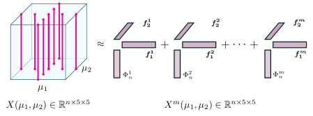
Figure 1: Example of tensor matrix $X(\mu_{1},\mu_{2})$ consisting of 9 snapshot solutions (dots connected by vertical lines) and reduced order model $X^{m}(\mu_{1},\mu_{2})$ of rank $m$ as in (22), where $\Phi_{n}^{k}\in\mathbb{R}^{n}$, $\bm{f_{1}^{k}}\coloneqq\begin{bmatrix}F_{1}^{k}(\mu_{1}^{1}),\ldots,F_{1}^{k}(\mu_{1}^{5})\end{bmatrix}\in\mathbb{R}^{5}$, $\bm{f_{2}^{k}}\coloneqq\begin{bmatrix}F_{2}^{k}(\mu_{2}^{1}),\ldots,F_{2}^{k}(\mu_{2}^{5})\end{bmatrix}\in\mathbb{R}^{5}$. Approximation is sum of rank-one tensors.

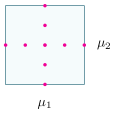
Figure 2: Sparse grid sampling in the parameter space. Nodes (21) correspond to the 9 snapshot solutions in Figure 1 with $\mu_{1}\in[a_{1},b_{1}]$, $\mu_{2}\in[a_{2},b_{2}]$, $\mu_{1}^{*}=(a_{1}+b_{1})/2$, $\mu_{2}^{*}=(a_{2}+b_{2})/2$. All snapshots generated via two executions of Preconditioned Chebyshev BiCG.

Sparse grid based higher order proper generalized decomposition (HOPGD) [35] is a method which generates an approximation $X^{m}(\mu_{1},\mu_{2})\in\mathbb{R}^{n\times n_{1}\times n_{2}}$ to the tensor matrix $X(\mu_{1},\mu_{2})\in\mathbb{R}^{n\times n_{1}\times n_{2}}$ (20). Specifically, this expression is separated in the parameters $\mu_{1}$ and $\mu_{2}$ and is of the form

(22a) $$X(\mu_{1}^{i},\mu_{2}^{*})\approx X^{m}(\mu_{1}^{i},\mu_{2}^{*}) =\sum_{k=1}^{m}\Phi_{n}^{k}F_{1}^{k}(\mu_{1}^{i})F_{2}^{k}(\mu_{2}^{*})\in\mathbb{R}^{n},\quad i =1,\ldots,n_{1},$$

(22b) $$X(\mu_{1}^{*},\mu_{2}^{j})\approx X^{m}(\mu_{1}^{*},\mu_{2}^{j}) =\sum_{k=1}^{m}\Phi_{n}^{k}F_{1}^{k}(\mu_{1}^{*})F_{2}^{k}(\mu_{2}^{j})\in\mathbb{R}^{n},\quad j =1,\ldots,n_{2}$$

at each node in the set (21), where $\Phi_{n}^{k}\in\mathbb{R}^{n}$ and

(23) $$F_{1}^{k}:\mathbb{R}\rightarrow\mathbb{R},\quad F_{2}^{k}:\mathbb{R}\rightarrow\mathbb{R}$$

are one variable scalar functions of the parameters $\mu_{1}$ and $\mu_{2}$, respectively. Here $m$ is the rank of the approximation and $F_{l}^{k}$, $l=1,2$, are the unknown functions of the $k$th mode. In this way, the original function $X(\mu_{1},\mu_{2})$, evaluated at the nodes $\bm{\mu}$, is estimated by a linear combination of products of lower-dimensional functions.

The decomposition in (22) generates only the evaluations of $F_{l}^{k}$, and the reduced basis vectors for the approximation are not known a priori. Instead, these vectors are determined on-the-fly, in contrast to other methods based on the similar proper orthogonal decomposition [9, 14]. A visualization of this decomposition on a sparse tensor of snapshots appears in Figure 1. The spacing of the nodes is equidistant in both the $\mu_{1}$ and $\mu_{2}$ directions, conventional for methods of this type.

We note the similarity between this method and the well-known higher-order singular value decomposition (HOSVD) [34]. Additionally, the reduced order model generated via the method sparse grid based HOPGD and visualized in Figure 1 is of the same form as the established CANDECOMP/PARAFAC (CP) decomposition. Specifically, the approximations consists of a sum of rank-one tensors [30].

The model as expressed in (22) can only be evaluated on the set of nodes (21) corresponding to the snapshots included in the tensor matrix (20). To access other approximations, interpolations of $F_{l}^{k}$ will be required; see Section 3.2. The particular structure of the sparse grid sampling incorporated here is very similar to that which is used in traditional sparse grid methods for PDEs [12]. Our approach differs from these methods, which are based on an interpolation of high dimensional functions using a hierarchical basis not considered here. See also [11] for a method in this style, where a reduced order model was constructed using hierarchical collocation to solve parameteric problems.

Remark 5 (Evaluation of the model at a point in space).

The approximation in (22) is expressed using vectors of length $n$ as the examples which follow in Sections 4 concern a parameterized PDE discretized on a spatial domain denoted by $\Omega$. In particular, we are interested in the solutions to these PDEs for many values of the parameters $\mu_{1}$ and $\mu_{2}$. The approximation (22), expressed at a point in space, is denoted by

(24) $$X(x_{0},\mu_{1},\mu_{2})\approx X^{m}(x_{0},\mu_{1},\mu_{2})=\sum_{k=1}^{m}\Phi^{k}(x_{0})F_{1}^{k}(\mu_{1})F_{2}^{k}(\mu_{2})\in\mathbb{R},$$

for a particular $(\mu_{1},\mu_{2})\in\bm{\mu}$ (21), where $x_{0}\in\Omega\subset\mathbb{R}^{d}$ is a spatial parameter, $d$ is the dimension of the spatial domain, and $\Phi^{k}(x_{0})\in\mathbb{R}$ is an entry of the vector $\Phi_{n}^{k}\in\mathbb{R}^{n}$ in (22). Specifically, $\Phi_{n}^{k}$ denotes $\Phi^{k}$ evaluated on a set of $n$ spatial discretization points $\Omega_{dp}$, where $\Omega_{dp}\subset\Omega$. As in (22), to evaluate the model in (24) for values of $\mu_{1}$ and $\mu_{2}$ outside of the set of nodes, interpolations must be performed.

3.1 Computation of the separated expression

Traditionally, tensor decomposition methods require sampling performed on full grids in the parameter space, requiring the computation and storage of many snapshot solutions. See [10, 36, 38] for HOPGD performed in this setting, as well as an example in Section 4.2. The tensor decomposition proposed in [35] is specifically designed for sparse tensors. In particular, the sampling is of the same form considered in Section 2 and shown in Figures 1 and 2. This approach is more efficient, as it requires fewer snapshots and, as a result, the decomposition is performed in fewer computations. The method in [35], adapted to our particular setting, is summarized here, and details on the full derivation appear in Appendix A.

We seek an approximation to the nonzero vertical columns of $X(\mu_{1},\mu_{2})$ described in (20), separated in the parameters $\mu_{1}\in[a_{1},b_{1}]$ and $\mu_{2}\in[a_{2},b_{2}]$. The full parameter domain is defined by $\mathcal{D}\coloneqq\Omega_{n}\times[a_{1},b_{1}]\times[a_{2},b_{2}]$, where $\Omega_{n}\subset\mathbb{R}^{n}$. We express solutions as vectors of length $n$, i.e., as approximations to (1) evaluated at a particular node $(\mu_{1},\mu_{2})$; cf. (24), where solutions are expressed at a single point in the spatial domain. The approximations satisfy

(25a) $$X(\mu_{1},\mu_{2}) \approx X^{m}(\mu_{1},\mu_{2}),$$

(25b) $$= \sum_{k=1}^{m}\Phi_{n}^{k}F_{1}^{k}(\mu_{1})F_{2}^{k}(\mu_{2}),$$

(25c) $$= X^{m-1}(\mu_{1},\mu_{2})+\Phi_{n}^{m}F_{1}^{m}(\mu_{1})F_{2}^{m}(\mu_{2}),$$

for $(\mu_{1},\mu_{2})\in\bm{\mu}$, where $\bm{\mu}$ is the set of nodes defined in (21), and are generated via an alternating directions strategy. Specifically, at each enrichment step $m$, all components $\Phi_{n}^{m}\in\mathbb{R}^{n}$, $F_{1}^{m}(\mu_{1})\in\mathbb{R}$, $F_{2}^{m}(\mu_{2})\in\mathbb{R}$ in (25c) are initialized then updated sequentially to construct an $L^{2}$ projection of $X(\mu_{1},\mu_{2})$. This is done via a greedy algorithm, where all components are assumed fixed, except the one we seek to compute. The process is equivalent to the minimization problem described as follows. At step $m$, find $X^{m}(\mu_{1},\mu_{2})\in V_{m}\subset L^{2}(\mathcal{D})$ as in (25) such that

(26) $$\min_{X^{m}(\mu_{1},\mu_{2})}\left(\frac{1}{2}\left\lVert wX(\mu_{1},\mu_{2})-wX^{m}(\mu_{1},\mu_{2})\right\rVert_{L^{2}(\mathcal{D})}^{2}\right),$$

where $w$ is the sampling index, i.e.,

$$\begin{cases}w=1,&(\mu_{1},\mu_{2})\in\bm{\mu},\\ w=0,&\text{otherwise},\end{cases}$$

$\mathcal{D}$ is the full parameter domain, and $V_{m}$ represents a set of test functions. Equivalently, using the weak formulation, we seek the solution $X^{m}(\mu_{1},\mu_{2})$ to

(27) $$(wX^{m}(\mu_{1},\mu_{2}),\delta X)_{\mathcal{D}}=(wX(\mu_{1},\mu_{2}),\delta X)_{\mathcal{D}},\quad\forall\delta X\in V_{m}.$$

Here $(\cdot,\cdot)_{\mathcal{D}}$ denotes the integral of the scalar product over the domain $\mathcal{D}$, and (27) can be written as

(28) $$\left(w\Phi_{n}^{m}F_{1}^{m}F_{2}^{m},\delta X\right)_{\mathcal{D}}=\left(wX(\mu_{1},\mu_{2})-wX^{m-1}(\mu_{1},\mu_{2}),\delta X\right)_{\mathcal{D}},\quad\forall\delta X\in V_{m};$$

see details in Appendix A. We have simplified the notation in (28) with $F_{1}^{m}\coloneqq F_{1}^{m}(\mu_{1})$ and $F_{2}^{m}\coloneqq F_{2}^{m}(\mu_{2})$ for readability. In practice, approximations to (28) are computed successively via a least squares procedure until a fixed point is detected. The $m$th test function is given by $\delta X\coloneqq\delta\Phi^{m}F_{1}^{m}F_{2}^{m}+\Phi_{n}^{m}\delta F_{1}^{m}F_{2}^{m}+\Phi_{n}^{m}F_{1}^{m}\delta F_{2}^{m}$, and the approximation (25c) is updated with the resulting components.

More concretely, let the initializations $\Phi_{n}^{m}$, $\bm{f_{1}^{m}}\coloneqq\begin{bmatrix}F_{1}^{m}(\mu_{1}^{1}),\ldots,F_{1}^{m}(\mu_{1}^{n_{1}})\end{bmatrix}\in\mathbb{R}^{n_{1}}$, $\bm{f_{2}^{m}}\coloneqq\begin{bmatrix}F_{2}^{m}(\mu_{2}^{1}),\ldots,F_{2}^{m}(\mu_{2}^{n_{2}})\end{bmatrix}\in\mathbb{R}^{n_{2}}$ be given. We seek first an update of $\Phi_{n}^{m_{\text{old}}}\coloneqq\Phi_{n}^{m}$, assuming $F_{1}^{m_{\text{old}}}\coloneqq F_{1}^{m}$, $F_{2}^{m_{\text{old}}}\coloneqq F_{2}^{m}$ are known function evaluations for all $(\mu_{1},\mu_{2})\in\bm{\mu}$. We update $\Phi_{n}^{m}$ as

(29) $$\Phi_{n}^{m}=\frac{\sum_{\bm{\mu}}r_{m-1}(\mu_{1},\mu_{2})}{\sum_{\bm{\mu}}F_{1}^{m}(\mu_{1})F_{2}^{m}(\mu_{2})},$$

where the $(m-1)$th residual vector is given by

(30) $$r_{m-1}(\mu_{1},\mu_{2})\coloneqq X(\mu_{1},\mu_{2})-X^{m-1}(\mu_{1},\mu_{2})\in\mathbb{R}^{n}.$$

Denote the vector obtained in (29) by $\Phi_{n}^{m_{\text{new}}}$ and seek an update of $F_{1}^{m_{\text{old}}}(\mu_{1}^{i})$, assuming $\Phi_{n}^{m}$, $F_{2}^{m}(\mu_{2}^{j})$ known, using

(31) $$F_{1}^{m}(\mu_{1}^{i})=\frac{(\Phi_{n}^{m})^{T}r_{m-1}(\mu_{1}^{i},\mu_{2}^{*})}{(\Phi_{n}^{m})^{T}\Phi_{n}^{m}F_{2}^{m}(\mu_{2}^{*})},$$

for $i=1,\ldots,n_{1}$. We denote the solutions found in (31) by $F_{1}^{m_{\text{new}}}(\mu_{1}^{i})$. Note, $\Phi_{n}^{m_{\text{new}}}$ and $F_{2}^{m_{\text{old}}}(\mu_{2}^{j})$ are used in the computations in (31). The updates $F_{2}^{m}(\mu_{2}^{j})$ are computed as

(32) $$F_{2}^{m}(\mu_{2}^{j})=\frac{(\Phi_{n}^{m})^{T}r_{m-1}(\mu_{1}^{*},\mu_{2}^{j})}{(\Phi_{n}^{m})^{T}\Phi_{n}^{m}F_{2}^{m}(\mu_{2}^{j})},$$

for $j=1,\ldots,n_{2}$, which we denote by $F_{2}^{m_{\text{new}}}(\mu_{2}^{j})$, where $\Phi_{n}^{m_{\text{new}}}$ and $F_{1}^{m_{\text{new}}}(\mu_{1}^{i})$ were used in the computations in (32). For a certain tolerance level $\varepsilon_{1}$, if the relation

(33) $$\left\lVert\delta(\mu_{1},\mu_{2})\right\rVert<\varepsilon_{1}$$

holds for all $(\mu_{1},\mu_{2})\in\bm{\mu}$, where

(34) $$\delta(\mu_{1},\mu_{2})\coloneqq\Phi_{n}^{m_{\text{old}}}F_{1}^{m_{\text{old}}}(\mu_{1})F_{2}^{m_{\text{old}}}(\mu_{2})-\Phi_{n}^{m_{\text{new}}}F_{1}^{m_{\text{new}}}(\mu_{1})F_{2}^{m_{\text{new}}}(\mu_{2}),$$

we have approached a fixed point. In this case, the approximation in (25c) is updated with the components $\Phi_{n}^{m}$, $F_{1}^{m}(\mu_{1}^{i})$, and $F_{2}^{m}(\mu_{2}^{j})$. If the condition (33) is not met, we set $\Phi_{n}^{m_{\text{old}}}\coloneqq\Phi_{n}^{m_{\text{new}}}$, $F_{1}^{m_{\text{old}}}(\mu_{1}^{i})\coloneqq F_{1}^{m_{\text{new}}}(\mu_{1}^{i})$, $F_{2}^{m_{\text{old}}}(\mu_{2}^{j})\coloneqq F_{2}^{m_{\text{new}}}(\mu_{2}^{j})$ and repeat the process described above. If

$$\frac{\left\lVert X(\mu_{1},\mu_{2})-X^{m}(\mu_{1},\mu_{2})\right\rVert}{\left\lVert X(\mu_{1},\mu_{2})\right\rVert}<\varepsilon_{2}$$

is met for a specified $\varepsilon_{2}$ and all $(\mu_{1},\mu_{2})\in\bm{\mu}$, the algorithm terminates. Otherwise, we seek $\Phi_{n}^{m+1}$, $F_{1}^{m+1}(\mu_{1}^{i})$, $F_{2}^{m+1}(\mu_{2}^{j})$ using the same procedure, initialized with the most recent updates. This process is summarized in Algorithm 1.

The most expensive operations in Algorithm 1 are the inner products of two vectors of dimension $n$, and, thus, the cost of each step in the tensor decomposition scales linearly with the number of unknowns in (1). In general, decompositions of many sets of snapshots can be performed to an acceptable accuracy level with $m\ll n$, where the parameter $m$ depends on the regularity of the exact solution [14]. Efficiency and robustness have been shown for the standard PGD method generated with a greedy algorithm like the one described here [15, 36, 41]. Note, the accuracy of the approximations here depends strongly on the quality of the separated functions in the model [35]. Additionally, the decomposition produced by the standard HOPGD method is optimal when the separation involves two parameters [38].

The reduced order model described here can be used to approximate solutions to (1) for many $(\mu_{1},\mu_{2})$ outside of the set of nodes. This is achieved through interpolating the one variable functions in (23). Consider also a solution vector $x(\mu_{1},\mu_{2})\in\mathbb{R}^{n}$ to (1), where $(\mu_{1},\mu_{2})$ are unknown. The interpolation of $X^{m}(\mu_{1},\mu_{2})$ can be used to estimate the parameters $\mu_{1}$, $\mu_{2}$ which produce this particular solution.

Remark 6 (Separated expression in more than two parameters).

The reduced order model (22) is separated in the two parameters $\mu_{1}$ and $\mu_{2}$. In [35], models separated in as many as six parameters were constructed, where the sampling was performed on a sparse grid in the parameter space. The authors note this particular approach for the decomposition may not be optimal in the sense of finding the best approximation, though it is possible. Our proposed way of computing the snapshots could be generalized to a setting separated in $s$ parameters. In this way, the procedure would fix $(s-1)$ parameters at a time and execute Chebyshev BiCG a total of $s$ times.

Remark 7 (Comparison of HOPGD to similar methods).

In [38], HOPGD was studied alongside the similar HOSVD method. The decompositions were separated in as many as six parameters, and the sampling was performed on a full grid in the parameter space. In general, HOPGD produced separable representations with fewer terms compared with HOSVD. In this way, the model constructed by HOPGD can be evaluated in a more efficient manner. Furthermore, the method HOPGD does not require the number of terms in the separated solution to be set a priori, as in a CP decomposition.

Input: Set of nodes $\bm{\mu}$ as in (21), tensor matrix of precomputed snapshots $X(\mu_{1},\mu_{2})$ as in (22), tolerances $\varepsilon_{1},\varepsilon_{2}>0$

Output: Function $\bm{X}^{m}(\mu_{1},\mu_{2}):[a_{1},b_{1}]\times[a_{2},b_{2}]\rightarrow\mathbb{R}^{n}$, approx to (1)

Initialize: $\Phi_{n}^{1}\in\mathbb{R}^{n}$, $F_{1}^{1}(\mu_{1}^{i})\in\mathbb{R}$, $F_{2}^{1}(\mu_{2}^{j})\in\mathbb{R}$, $i=1,\ldots,n_{1}$, $j=1,\ldots,n_{2}$

1 $m=1$

2 Set $X^{0}(\mu_{1}^{i},\mu_{2}^{j})\coloneqq 0$, $X^{m}(\mu_{1}^{i},\mu_{2}^{j})\coloneqq\Phi_{n}^{m}F_{1}^{m}(\mu_{1}^{i})F_{2}^{m}(\mu_{2}^{j})$

3 while $\left\lVert X(\mu_{1},\mu_{2})-X^{m}(\mu_{1},\mu_{2})\right\rVert/\left\lVert X(\mu_{1},\mu_{2})\right\rVert>\varepsilon_{2}$, for any $(\mu_{1},\mu_{2})\in\bm{\mu}$ do

4       Set $\Phi_{n}^{m_{\text{old}}}\coloneqq\Phi_{n}^{m}$, $F_{1}^{m_{\text{old}}}(\mu_{1}^{i})\coloneqq F_{1}^{m}(\mu_{1}^{i})$, $F_{2}^{m_{\text{old}}}(\mu_{2}^{j})\coloneqq F_{2}^{m}(\mu_{2}^{j})$

5       Compute $\Phi_{n}^{m}$ with (29)

6       Set $\Phi_{n}^{m_{\text{new}}}\coloneqq\Phi_{n}^{m}$

7       Compute $F_{1}^{m}(\mu_{1}^{i})$ with (31)

8       Set $F_{1}^{m_{\text{new}}}(\mu_{1}^{i})\coloneqq F_{1}^{m}(\mu_{1}^{i})$

9       Compute $F_{2}^{m}(\mu_{2}^{j})$ with (32)

10       Set $F_{2}^{m_{\text{new}}}(\mu_{2}^{j})\coloneqq F_{2}^{m}(\mu_{2}^{j})$

11       Compute $\delta(\mu_{1}^{i},\mu_{2}^{j})$ (34)

12       if $\delta(\mu_{1},\mu_{2})<\varepsilon_{1}$, for all $(\mu_{1},\mu_{2})\in\bm{\mu}$ do

13             Update $X^{m}(\mu_{1},\mu_{2})$ as in (25c)

14             Set $m\coloneqq m+1$

15             Set $\Phi_{n}^{m}\coloneqq\Phi_{n}^{m-1}$, $F_{1}^{m}(\mu_{1}^{i})\coloneqq F_{1}^{m-1}(\mu_{1}^{i})$, $F_{2}^{m}(\mu_{2}^{j})\coloneqq F_{2}^{m-1}(\mu_{2}^{j})$

16       end

17      

18 end while

return Compute interpolation $\bm{X}^{m}(\mu_{1},\mu_{2})$ as in (35)

Algorithm 1 Sparse grid based Chebyshev HOPGD for parameterized linear systems

3.2 Interpolated model

The tensor representation in (22) consists, in part, of one-dimensional functions $F_{1}^{k}$ and $F_{2}^{k}$, for $k=1,\ldots,m$. Note, we have only evaluations of these functions at $\mu_{1}^{i}$, $i=1,\ldots,n_{1}$ and $\mu_{2}^{j}$, $j=1,\ldots,n_{2}$, respectively, and no information about these functions outside of these points. In this way, we cannot approximate the solution to (1) for all $(\mu_{1},\mu_{2})\in[a_{1},b_{1}]\times[a_{2},b_{2}]$ using (22) as written.

We can use the evaluations $F_{1}^{k}(\mu_{1}^{i})$ and $F_{2}^{k}(\mu_{2}^{j})$ in (22) to compute an interpolation of these one-dimensional functions in a cheap way. In practice, any interpolation is possible and varying the type of interpolation does not contribute significantly to the overall error in the approximation. Thus, we make the following interpolation of the representation in (22):

(35) $$\bm{X}^{m}(\mu_{1},\mu_{2}) =\sum_{k=1}^{m}\Phi_{n}^{k}\bm{F}_{1}^{k}(\mu_{1})\bm{F}_{2}^{k}(\mu_{2})\in\mathbb{R}^{n},$$

where $\bm{F}_{1}^{k}$, $\bm{F}_{2}^{k}$ are spline interpolations of $F_{1}^{k}$, $F_{2}^{k}$ (23), respectively, and $\bm{X}^{m}(\mu_{1},\mu_{2}):[a_{1},b_{1}]\times[a_{2},b_{2}]\rightarrow\mathbb{R}^{n}$. The interpolation in (35) can be evaluated to approximate (1) for other $(\mu_{1},\mu_{2})\in[a_{1},b_{1}]\times[a_{2},b_{2}]$ in a cheap way. This approximation to $x(\mu_{1},\mu_{2})$ is denoted as

(36) $$x^{m}(\mu_{1},\mu_{2})\in\mathbb{R}^{n},$$

and we compute the corresponding relative error as follows:

$$\frac{\left\lVert x^{m}(\mu_{1},\mu_{2})-x(\mu_{1},\mu_{2})\right\rVert_{2}}{\left\lVert x(\mu_{1},\mu_{2})\right\rVert_{2}}\cdot$$

Note, simply interpolating several snapshots to estimate solutions to (1) for all $(\mu_{1},\mu_{2})$ in the parameter space is not a suitable approach, as the solutions tend to be extremely sensitive to the parameters [38].

To solve the parameter estimation problem for a given solution $x(\mu_{1},\mu_{2})\in\mathbb{R}^{n}$ which depends on unknown parameters $(\mu_{1},\mu_{2})$, we use the Matlab routine fmincon which uses the sequential quadratic programming algorithm [40] to find the pair of values $(\mu_{1},\mu_{2})$ in the the domain which minimize the quantity

(37) $$\left\lVert x(\mu_{1},\mu_{2})-x^{m}(\mu_{1},\mu_{2})\right\rVert_{2}.$$

Simulations from a parameterized Helmholtz equation and a parameterized advection-diffusion equation appear in Sections 4 and 5, respectively. In these experiments, an interpolation of a reduced order model is constructed to approximate the solutions to the parameterized PDEs.

Remark 8 (Offline and online stages).

In practice, the fixed point method in Algorithm 1 can require many iterations until convergence, though the cost of each step scales linearly with the number of unknowns. Residual-based accelerators have been studied to reduce the number of these iterations [35]. This strategy, though outside the scope of this work, has shown to be beneficial in situations where the snapshots depended strongly on the parameters. Only one successful decomposition is required to construct (35). Thus, the offline stage of the method consists of generating the snapshots with Chebyshev BiCG and executing Algorithm 1.

Evaluating the reduced order model (35) requires only scalar and vector operations and, therefore, a variety of approximations to (1) can be obtained very quickly, even when the number of unknowns is large. We consider this part of the proposed method the online stage. In the experiment corresponding to Figure 7, evaluating the reduced order model had simulation time $0.010601$ CPU seconds. Generating the corresponding finite element solution with backslash in Matlab had simulation time $1.197930$ CPU seconds.

Remark 9 (Sources of error).

The approximations generated by Algorithm 1 contain error from the Chebyshev approximation, the iterative method Preconditioned Chebyshev BiCG, the low-rank approximation, as well as the interpolations in (35). As noted in Remark 4, the Chebyshev approximation has a very small impact on the overall error, and Figure 4 shows that the iterative method obtains relatively accurate approximations to the true solutions. In practice, the interpolations performed in (35) are done on smooth functions, as visualized in Figure 5. The largest source of error from our proposed algorithm stems from the tensor decomposition, i.e., lines $1$–$17$ in Algorithm 1. This can be seen, for example, in Figure 6.

4 Numerical simulations of a parameterized Helmholtz equation

We consider both a reduced order model for a parameterized Helmholtz equation and a parameter estimation problem for the solution to a parameterized Helmholtz equation. Such settings occur naturally, for example, in the study of geophysics; see [38, 43, 47]. These prior works were also based on a reduced order model, constructed using PGD. Similarly, the method PGD was used in the study of thermal process in [1], and a reduced basis method for solving parameterized PDEs was considered in [27].

In the simulations which follow, the matrices $A_{i}$ arise from a finite element discretization, and $b$ is the corresponding load vector. All matrices and vectors here were generated using the finite element software FEniCS [3]. The solutions to these discretized systems were approximated with a modified version of the Kryov subspace method Preconditioned Chebyshev BiCG [17], as described in Section 2. This strategy requires a linear solve with a matrix of dimension $n\times n$ on each application of the preconditioner and of its adjoint. We have chosen to perform the linear solve by computing one LU decomposition per execution of the main algorithm, which is reused at each subsequent iteration accordingly. This can be avoided by considering the inexact version of Preconditioned Chebyshev BiCG; see Remark 2.

This work proposes a novel improvement in generating snapshot solutions necessary for constructing models of this type. We choose to include three different examples in this section in order to fully capture the versatility of our strategy. Once the interpolation (35) has been constructed, evaluating the approximations for many values of the parameters $\mu_{1}$ and $\mu_{2}$ can be done in an efficient manner; see Remark 8. In the case of the tensor decomposition failing to converge sufficiently, a new set of snapshots can be generated with little extra work and a new decomposition can be attempted; see Section 2.

4.1 First simulation, snapshots on a sparse grid

Consider the Helmholtz equation given by

(38a) $$\nabla^{2}u(x)+f(\mu_{1},\mu_{2})u(x) =h(x),\quad x\in\Omega,$$

(38b) $$u(x) =0,\quad x\in\partial\Omega,$$

where $\Omega\subset\mathbb{R}^{2}$ is as in Figure 7, $\mu_{1}\in[1,2]$, $\mu_{2}\in[1,2]$, $f(\mu_{1},\mu_{2})=2\pi^{2}+\cos(\mu_{1})+\mu_{1}^{4}+\sin(\mu_{2})+\mu_{2}$, and $h(x)=\sin(\pi x_{1})\sin(\pi x_{2})$. A discretization of (38) is of the form (1), where

$$A(\mu_{1},\mu_{2})\coloneqq A_{0}+f(\mu_{1},\mu_{2})A_{1}.$$

We are interested in approximating $u(x)$ in (38) for many different pairs of $(\mu_{1},\mu_{2})$ simultaneously.

The reduced order model $\bm{X}^{m}(\mu_{1},\mu_{2})$ is constructed as described in Algorithm 1. We can evaluate this model for $(\mu_{1},\mu_{2})$ outside of the nodes corresponding to the snapshot solutions. The particular $13$ nodes considered in this simulation are plotted in the parameter space, shown in Figure 3. Figure 4 displays the convergence of the two executions of Preconditioned Chebyshev BiCG required to generate the snapshot corresponding to the nodes in Figure 3. Specifically, in Figure 4(a), we see faster convergence for approximations $\hat{x}(\mu_{1},\mu_{2}^{*})$ where the value $\mu_{1}$ is closer to the target parameter $\hat{\sigma}$ in (9). An analogous result holds in Figure 4(b) for approximations $\tilde{x}(\mu_{1}^{*},\mu_{2})$ where $\mu_{2}$ is closer to $\tilde{\sigma}$; see Remark 1. We require the LU decompositions of $2$ different matrices of dimension $n\times n$ for this simulation.

In Figure 5, we see the interpolations $\bm{F}_{1}^{1}(\mu_{1})$ and $\bm{F}_{2}^{1}(\mu_{2})$ as in (35) plotted along with the function evaluations $F_{1}^{1}(\mu_{1}^{i})$ and $F_{2}^{1}(\mu_{2}^{j})$ generated by Algorithm 1, where $\mu_{1}^{i}$ and $\mu_{2}^{j}$ are as in Figure 3. Figure 6 shows the percent relative error for approximations to (38) for a variety of pairs $(\mu_{1},\mu_{2})$ different from the nodes plotted in Figure 3. As in [36], we consider approximate solutions with percent relative error below $6\%$ reliable and approximations with percent relative error below $1.5\%$ accurate, where the error is computed by comparing the approximation to the solution obtained using backslash in Matlab. Figures 7, 8, and 9 show both the finite element solution and the solution generated from (35) for the sake of comparison. Here we display these solutions for $3$ pairs of $(\mu_{1},\mu_{2})$. These approximations all have percent relative error below $1.5\%$. A variety of solutions can be obtained from this reduced order model.

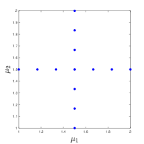
Figure 3: Locations of $13$ snapshots $(\mu_{1}^{i},\mu_{2}^{*})$ and $(\mu_{1}^{*},\mu_{2}^{j})$ used to construct $X^{m}$ in (22) to approximate (38), sampling on a sparse grid in the parameter space.

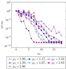
(a) Approximations to (6) with target parameter $\hat{\sigma}=1.48$ as in (9), fixed parameter $\mu_{2}^{*}=1.5$.

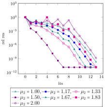
(b) Approximations to (19) with target parameter $\tilde{\sigma}=1.48$, analogous to $\hat{\sigma}$ in (9), fixed parameter $\mu_{1}^{*}=1.5$.

Figure 4: Convergence of Preconditioned Chebyshev BiCG for generating the snapshot solutions corresponding to the nodes in Figure 3. Simulation in Figure 4(a) gives all solutions for $(\mu_{1},\mu_{2}^{*})$, $\mu_{1}\in[1,2]$, simulation in Figure 4(b) gives all solutions for $(\mu_{1}^{*},\mu_{2})$, $\mu_{2}\in[1,2]$.

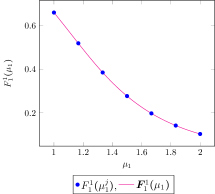
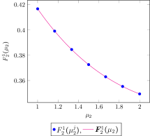
Figure 5: Function evaluations $F_{1}^{1}(\mu_{1}^{i})$ and $F_{2}^{1}(\mu_{2}^{j})$ produced by Algorithm 1 to approximate (38), plotted with corresponding interpolations $\bm{F}_{1}^{1}(\mu_{1})$ and $\bm{F}_{2}^{1}(\mu_{2})$ as in (35) with $\mu_{1}^{i}$ and $\mu_{2}^{j}$ as in Figure 3.

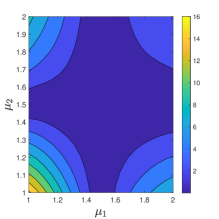
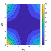
Figure 6: Percent relative error of $x^{m}(\mu_{1},\mu_{2})$ (36) to approximate (38) for 400 equidistant pairs of $(\mu_{1},\mu_{2})$, $m=14$, $n=112995$. Here accurate: $<1.5\%$, reliable: $<6\%$. Note, same model in both figures.

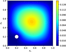
(a) Finite element solution

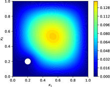
(b) Reduced order model solution

Figure 7: Approximation to (38) with $m=14$, $n=112995$, $.347\%$ relative error (accurate), $\mu_{1}=1.6$, $\mu_{2}=1.4$.

(a) Finite element solution

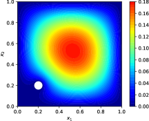
(b) Reduced order model solution

Figure 8: Approximation to (38) with $m=14$, $n=112995$, $.171\%$ relative error (accurate), $\mu_{1}=1.45$, $\mu_{2}=1.6$.

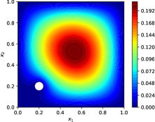
(a) Finite element solution

(b) Reduced order model solution

Figure 9: Approximation to (38) with $m=14$, $n=112995$, $0.414\%$ relative error (accurate), $\mu_{1}=1.4$, $\mu_{2}=1.4$.

4.2 Second simulation, snapshots on a full grid

To obtain an accurate model over the entire parameter space, we consider using HOPGD with sampling performed on a full grid. This is the approach taken in [10, 36] to approximate parametric PDEs. The snapshots are obtained using the Krylov subspace method described in Section 2, and the model is constructed in a way that is completely analogous to the method described in Section 3. As the decomposition is performed on a tensor matrix containing more snapshots, the method is more costly.

Specifically, we build a reduced order model to approximate the solution to the Helmholtz equation given by

(39a) $$\left(\nabla^{2}+f_{1}(\mu_{1})+f_{2}(\mu_{2})\alpha(x)\right)u(x) =h(x),\quad x\in\Omega,$$

(39b) $$u(x) =0,\quad x\in\partial\Omega,$$

where $\Omega\subset\mathbb{R}^{2}$ is as in Figure 11, $\alpha(x)=x_{2}$, $\mu_{1}\in[1,2]$, $\mu_{2}\in[1,2]$, and $f_{1}(\mu_{1})=\cos(\mu_{1})+\mu_{1}^{3}$, $f_{2}(\mu_{2})=\sin(\mu_{2})+\mu_{2}^{2}$, $h(x)=\sin(\pi x_{1})\sin(\pi x_{2})$. A discretization of (39) is of the form (1), where

$$A(\mu_{1},\mu_{2})\coloneqq A_{0}+f_{1}(\mu_{1})A_{1}+f_{2}(\mu_{2})A_{2},$$

and approximating $u(x)$ in (40) for many different pairs of $(\mu_{1},\mu_{2})$ is of interest. We can still exploit the structure of the sampling when generating the snapshots by fixing one parameter and returning solutions as a one variable function of the other parameter. As in the simulations based on sparse grid sampling, if the decomposition fails to reach a certain accuracy level, a new set of snapshots can be generated with little extra computational effort.

Figure 10(a) shows the locations of the nodes corresponding to $77$ different snapshot solutions used to construct a reduced order model. These snapshots were generated via $7$ executions of a modified form of Preconditioned Chebyshev BiCG, i.e., we consider $7$ different fixed $\mu_{2}^{*}$, equally spaced on $[a_{2},b_{2}]$. This requires the LU decompositions of $7$ different matrices of size $n\times n$. Figure 10(b) shows the percent relative error of the interpolated approximation, analogous to (35) constructed using Algorithm 1, for $400$ pairs of $(\mu_{1},\mu_{2})\in[1,2]\times[1,2]$, different from the nodes corresponding to the snapshot solutions. We note that the percent relative error of the approximation is below $1\%$ for all pairs $(\mu_{1},\mu_{2})$, indicating that the approximations are accurate. For the sake of comparison, Figures 11, 12 and 13 show both the finite element solutions and corresponding reduced order model solutions for $3$ pairs of $(\mu_{1},\mu_{2})$. In general, accurate solutions can be produced on a larger parameter space with full grid sampling. Furthermore, the model can produce a variety of solutions.

(a) $77$ nodes, corresponding snapshots generated via $7$ executions of Preconditioned Chebyshev BiCG, $7$ fixed values $\mu_{2}^{*}$.

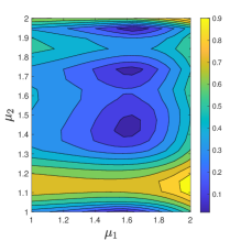
(b) Percent relative error of interpolation of reduced order model for 400 equidistant pairs of $(\mu_{1},\mu_{2})$.

Figure 10: Simulation for approximating (39). Here percent relative error $<1.5\%$ (accurate), $n=112693$, $m=16$, sampling on a full grid.

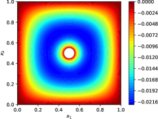
(a) Finite element solution

(b) Reduced order model solution

Figure 11: Approximation to (39) with $m=16$, $n=112693$, $.340\%$ relative error (accurate), $\mu_{1}=1$, $\mu_{2}=1$.

(a) Finite element solution

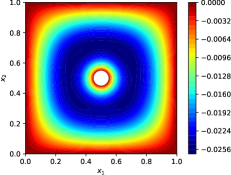
(b) Reduced order model solution

Figure 12: Approximation to (39) with $m=16$, $n=112693$, $.714\%$ relative error (accurate), $\mu_{1}=1.8$, $\mu_{2}=1.2$.

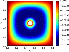
(a) Finite element solution

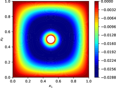
(b) Reduced order model solution

Figure 13: Approximation to (39) with $m=16$, $n=112693$, $.946\%$ relative error (accurate), $\mu_{1}=2$, $\mu_{2}=2$.

4.3 Third simulation, parameter estimation with snapshots on a sparse grid

We consider now an application of our method to solve a parameter estimation problem. Similar methods have been constructed in the context of parameterized PDEs, for example, [37, 39, 43]. Our approach is analogous to the experiments performed in [37], where several reduced order models were constructed using the method sparse grid based HOPGD [35]. Consider the Helmholtz equation given by

(40a) $$\left(\nabla^{2}+f_{1}(\mu_{1})+f_{2}(\mu_{2})\alpha(x)\right)u(x) =h(x),\quad x\in\Omega,$$

(40b) $$u(x) =0,\quad x\in\partial\Omega,$$

where $\Omega=[0,1]\times[0,1]$, $\alpha(x)=x_{1}$, $f_{1}(\mu_{1})=\sin^{2}(\mu_{1})$, $f_{2}(\mu_{2})=\cos^{2}(\mu_{2})$, $\mu_{1}\in[0,1]$, $\mu_{2}\in[0,1]$, and $h(x)=\exp(-x_{1}x_{2})$. A discretization of (40) is of the form (1), where

$$A(\mu_{1},\mu_{2})\coloneqq A_{0}+f_{1}(\mu_{1})A_{1}+f_{2}(\mu_{2})A_{2}.$$

We consider a parameter estimation problem, i.e., we have a solution to the discretized problem, where the parameters $(\mu_{1},\mu_{2})$ are unknown. In particular, the solution is obtained using backslash in Matlab.

Figures 14(a), 14(b), and 14(c) together show a method similar to the one proposed in [37] for approximating this problem, performed by constructing $3$ successive HOPGD models with sparse grid sampling. This simulation executes a modified form of Preconditioned Chebyshev BiCG $6$ times, requiring the LU factorizations of $6$ different matrices of dimension $n\times n$ to generate the $39$ snapshot solutions used to create the $3$ reduced order models. Once the models have been constructed, an interpolation is performed, followed by the minimization of (37). Table 1 shows the percent relative error in the estimated values of $\mu_{1}$ and $\mu_{2}$ for each run. Each execution of our strategy leads to a better estimation of the pair of parameters. As before, if the decomposition fails to reach a certain level of accuracy on a set of snapshots, a new set of approximations in the same parameter space can be generated with little extra computational effort.

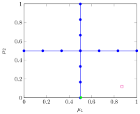
(a) First run, $m=34$.

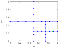
(b) Second run, $m=25$.

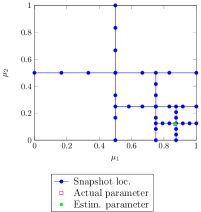
(c) Third run, $m=7$.

Figure 14: Parameter estimation for solution to (40), $n=10024$.

	rel err $\%$ $\mu_{1}$	rel err $\%$ $\mu_{2}$
First run, $m=34$	41.87417	97.40212
Second run, $m=25$	2.66555	105.09263
Third run, $m=7$	0.05706	1.69921

Table 1: Percent relative error for parameter estimation in $\mu_{1}$ and $\mu_{2}$ for solution to (40), $n=10024$.

5 Numerical simulations of a parameterized advection-diffusion equation

The advection-diffusion equation can be used to model particle transport, for example the distribution of air pollutants in the atmosphere; see [20, 46]. In particular, we consider the parameterized advection-diffusion equation given by

(41) $$\frac{\partial}{\partial t}u(x,t)=f_{1}(\mu_{1})\frac{\partial^{2}}{\partial x^{2}}u(x,t)+f_{2}(\mu_{2})\frac{\partial}{\partial x}u(x,t),$$

where $f_{1}(\mu_{1})=1+\sin(\mu_{1})$, $f_{2}(\mu_{2})=10+\cos(\mu_{2})+\pi\mu_{2}$ and $x\in[0,1]$, $t\in[0,T]$. The boundary conditions $u(0,t)=0$, $u(1,t)=0$ is enforced, as well as the initial condition $u_{0}(x)=u(x,0)=\sin(\pi x)$. Here the function evaluation $f_{1}(\mu_{1})$ is referred to as the diffusion coefficient, and the value $f_{2}(\mu_{2})$ is the advection parameter. Discretizing (41) in space, with a finite difference scheme, and in time, with by the implicit Euler method, gives a parameterized linear system of the form (1), where

$$A(\mu_{1},\mu_{2})\coloneqq A_{0}+f_{1}(\mu_{1})A_{1}+f_{2}(\mu_{2})A_{2}.$$

Note, the solution to this linear system gives an approximation to (41) at a specific time-step. As in Section 4, we construct a reduced order model via a tensor decomposition [35], where the snapshots are generated efficiently with a modified version of the method Preconditioned Chebyshev BiCG [17]. Here the sampling is performed on a sparse grid in the parameter space. If the tensor decomposition is not successful on a given set of snapshots, a new set can be generated on the same parameter space with little extra computation. Similar model problems appear in, for example, [41], where the method PGD was used to construct approximate solutions to the parameterized PDE. Once the corresponding reduced order model (35) has been constructed, approximating the solutions for many $(\mu_{1},\mu_{2})$ can be done very cheaply; see Remark 8.

5.1 First simulation, snapshots on a sparse grid

We construct approximations to (41) with Algorithm 1, where the sparse grid sampling is performed as displayed in Figure 16(a). Figure 15 shows the percent relative error for approximations to (41) for $400$ different pairs $(\mu_{1},\mu_{2})\in[0,0.5]\times[0,0.5]$, where, specifically, we consider the solutions at $t=0.01$. As in [36], approximate solutions with percent relative error below $6\%$ are considered reliable, and approximations with percent relative error below $1.5\%$ are considered accurate. Here the error is computed by comparing the approximation to the solution obtained using backslash in Matlab. The $9$ snapshots used to constructed the reduced order model here were generated with $2$ executions of Chebyshev BiCG, requiring the LU decompositions of $2$ matrices of dimension $n\times n$.

Note, solutions to the advection-diffusion equation (41) are time-dependent. An all-at-once procedure could be utilized to approximate solutions to this equation at many different time-steps, though this approach would result in a larger number of unknowns and a longer simulation time. Alternatively, the decomposition could be modified to construct an approximation similar to the one in (22), separated in the time variable $t$ as well as the parameters $\mu_{1}$ and $\mu_{2}$. Such an approach would, however, require specific testing. Furthermore, a decomposition of this form performed with HOPGD and sparse grid sampling in the parameter space may not be optimal [35].

Figure 15: Percent relative error of $x^{m}(\mu_{1},\mu_{2})$ (36) to approximate (41) for $400$ pairs of $(\mu_{1},\mu_{2})$, $m=50$, $n=9999$. Here accurate: $<1.5\%$, reliable $<6\%$. Note, same model in both figures.

5.2 Second simulation, parameter estimation with snapshots on a sparse grid

Consider again a parameter estimation problem. Specifically, we have an approximation to $u(x,t)\in\mathbb{R}^{n}$ in (41), where $t=0.01$ is known, but the parameters $\mu_{1}$ and $\mu_{2}$ are not. This approximation corresponds to the solution to the discretized problem and is obtained using backslash in Matlab. Additionally, there is some uncertainty in the measurement of the given solution. In this way, we express our observed solution $u^{\text{obs}}\in\mathbb{R}^{n}$ as

(42) $$u^{\text{obs}}\coloneqq u(x,t)+\varepsilon\Delta,$$

where $\Delta\in\mathcal{N}(0,I)\in\mathbb{R}^{n}$ is a random vector and $\varepsilon=10^{-2}$.

Figure 16 and Table 2 show the result of this parameter estimation problem, using a similar strategy to the one described in [37]. Here $3$ successive HOPGD models are constructed from snapshots sampled on a sparse grid in the parameter space $(\mu_{1},\mu_{2})\in[0,0.5]\times[0,0.5]$. This simulation executes a modified version of Chebyshev BiCG $6$ times, generating the $23$ snapshots efficiently. Note, this requires the LU decompositions of $6$ matrices of dimension $n\times n$. After the third run of Algorithm 1, the estimated parameter is very close to the actual parameter. Note, the relative error in $\mu_{1}$ and $\mu_{2}$ after the third run of the simulation is of the same order of magnitude as the noise in the observed solution (42).

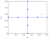
(a) First run, $m=50$.

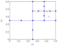
(b) Second run, $m=25$.

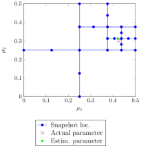
(c) Third run, $m=15$.

Figure 16: Parameter estimation for noisy solution to (41), $n=9999$.

	rel err $\%$ $\mu_{1}$	rel err $\%$ $\mu_{2}$
First run, $m=50$	1.9004	16.1248
Second run, $m=25$	4.8542	23.2504
Third run, $m=15$	1.2313	4.2588

Table 2: Percent relative error for parameter estimation in $\mu_{1}$ and $\mu_{2}$ for noisy solution to (41), $n=9999$.

6 Conclusions and future work

This work proposes a novel way to generate the snapshot solutions required to build a reduced order model. The model is based on an efficient decomposition of a tensor matrix, where the sampling is performed on a sparse grid. An adaptation of the previously proposed method Preconditioned Chebyshev BiCG is used to generate many snapshots simultaneously. Tensor decompositions may fail to reach a certain level of accuracy on a given set of snapshot solutions. Our approach offers a way to generate a new set of snapshots on the same parameter space with little extra computation. This is advantageous, as it is not possible to know a priori if a decomposition will converge or not on a given set of snapshots, and generating snapshots is computationally demanding in general. The reduced order model can also be used to solve a parameter estimation problem. Numerical simulations show competitive results.

In [35], a residual-based accelerator was used in order to decrease the number of iterations required by the fixed point method when computing the updates described in (29), (31), and (32). Techniques of this variety are especially effective when the snapshot solutions have a strong dependence on the parameters. Such a strategy could be directly incorporated into this work, though specific testing of the effectiveness would be required.

7 Acknowledgements

The Erasmus+ programme of the European Union funded the first author’s extended visit to Trinity College Dublin to carry out this research. The authors thank Elias Jarlebring (KTH Royal Institute of Technology) for fruitful discussions and for providing feedback on the manuscript. Additionally, the authors wish to thank Anna-Karin Tornberg (KTH Royal Institute of Technology) and her research group for many supportive, constructive discussions.

Appendix A Derivation of the update formulas, Algorithm 1

We are interested in the approximation $X^{m}(\mu_{1},\mu_{2})$ as in (25), such that (26) is satisfied. Here an alternating directions algorithm is used, where $X^{m-1}(\mu_{1},\mu_{2})$ as in (25c) is given, and we assume, after an initialization, $F_{1}^{m}\coloneqq F_{1}^{m}(\mu_{1})$, $F_{2}^{m}\coloneqq F_{2}^{m}(\mu_{2})$ are known. Equivalently, we seek the update $\Phi_{n}^{m}$ in (28) via a least squares procedure. The left-hand side of (28) can be expressed equivalently as

(43) $$\left(w\Phi_{n}^{m}F_{1}^{m}F_{2}^{m},\delta X\right)_{\mathcal{D}}=w\Phi_{n}^{m}(F_{1}^{m})^{2}(F_{2}^{m})^{2}\int_{\mathcal{D}}\delta\Phi^{m}(x)\mathop{dx}\mathop{d\mu_{1}}\mathop{d\mu_{2},}$$

and the right-hand side can be written as

(44) $$\left(wr_{m-1}(\mu_{1},\mu_{2}),\delta X\right)_{\mathcal{D}}=wr_{m-1}(\mu_{1},\mu_{2})F_{1}^{m}F_{2}^{m}\int_{\mathcal{D}}\delta\Phi^{m}(x)\mathop{dx}\mathop{d\mu_{1}}\mathop{d\mu_{2},}$$

with $r_{m-1}$ (30). Thus, from equating (43) and (44), we obtain the overdetermined system

(45) $$\begin{bmatrix}F_{1}^{m}(\mu_{1}^{1})F_{2}^{m}(\mu_{2}^{*})I_{n}\\ \vdots\\ F_{1}^{m}(\mu_{1}^{*})F_{2}^{m}(\mu_{2}^{n_{2}})I_{n}\end{bmatrix}\Phi^{m}_{n}=\begin{bmatrix}r_{m-1}(\mu_{1}^{1},\mu_{2}^{*})\\ \vdots\\ r_{m-1}(\mu_{1}^{*},\mu_{2}^{n_{2}})\end{bmatrix},$$

where $I_{n}\in\mathbb{R}^{n\times n}$ is the identity matrix of dimension $n$, and the update for $\Phi_{n}^{m}$ described in (29) is determined via the solution to the corresponding normal equations. Note, the linear system (45) contains function evaluations corresponding to all the nodes in $\bm{\mu}$ (21).

Assume now $\Phi_{n}^{m}$, $F_{2}^{m}$ in (25c) are known, and seek an update of $F_{1}^{m}$. Rewriting the left-hand side of (28) yields

(46) $$\left(w\Phi_{n}^{m}F_{1}^{m}F_{2}^{m},\delta X\right)_{\mathcal{D}}=w(\Phi_{n}^{m})^{T}(\Phi_{n}^{m})(F_{1}^{m})(F_{2}^{m})^{2}\int_{\mathcal{D}}\delta F_{1}^{m}(\mu_{1})\mathop{dx}\mathop{d\mu_{1}}\mathop{d\mu_{2},}$$

and the right-hand side is given by

(47) $$\left(wr_{m-1}(\mu_{1},\mu_{2}),\delta X\right)_{\mathcal{D}}=w(r_{m-1}(\mu_{1},\mu_{2}))^{T}(\Phi_{n}^{m})F_{2}^{m}\int_{\mathcal{D}}\delta F_{1}^{m}(\mu_{1})\mathop{dx}\mathop{d\mu_{1}}\mathop{d\mu_{2}\cdot}$$

Approximates to $F_{1}^{m}$ in (28) are found by computing the least squares solutions to the overdetermined systems

(48) $$\begin{bmatrix}\Phi_{n}^{m}F_{2}^{m}(\mu_{2}^{*})\end{bmatrix}F_{1}^{m}(\mu_{1}^{i})=\begin{bmatrix}r_{m-1}(\mu_{1}^{i},\mu_{2}^{*})\end{bmatrix},$$

given in (31). Proceeding analogously to (46) and (47), updating $F_{2}^{m}$ yields the overdetermined systems

(49) $$\begin{bmatrix}\Phi_{n}^{m}F_{1}^{m}(\mu_{1}^{*})\end{bmatrix}F_{2}^{m}(\mu_{2}^{j})=\begin{bmatrix}r_{m-1}(\mu_{1}^{*},\mu_{2}^{j})\end{bmatrix},$$

with least squares solutions (32).

In practice, each of the vectors depicted in the approximation in Figure 1 are normalized. A constant is computed for each low-rank update, in a process analogous to the one described above. We leave this out of the derivation for the sake of brevity. This is consistent with the algorithm derived in [35].

References

- [1] J. V. Aguado, A. Huerta, F. Chinesta, and E. Cueto, Real-time monitoring of thermal processes by reduced-order modeling, Internat. J. Numer. Methods Engrg., 102 (2015), pp. 991–1017.
- [2] M. I. Ahmad, D. B. Szyld, and M. B. van Gijzen, Preconditioned multishift BiCG for -optimal model reduction, SIAM J. Matrix Anal. Appl., 38 (2017), pp. 401–424.
- [3] M. S. Alnaes, J. Blechta, J. Hake, A. Johansson, B. Kehlet, A. Logg, C. Richardson, J. Ring, M. E. Rognes, and G. N. Wells, The FEniCS project version 1.5, Arch. Numer. Softw., 3 (2015).
- [4] A. Amiraslani, R. M. Corless, and P. Lancaster, Linearization of matrix polynomials expressed in polynomial bases, IMA J. Numer. Anal., 29 (2009), pp. 141–157.
- [5] A. Ammar, B. Mokdad, F. Chinesta, and R. Keunings, A new family of solvers for some classes of multidimensional partial differential equations encountered in kinetic theory modelling of complex fluids, J. Non-Newtonian Fluid Mech., 139 (2006), pp. 153–176.
- [6] , A new family of solvers for some classes of multidimensional partial differential equations encountered in kinetic theory modelling of complex fluids. Part II: Transient simulation using space-time separated representations, J. Non-Newtonian Fluid Mech., 144 (2007), pp. 98–121.
- [7] T. Bakhos, P. K. Kitanidis, S. Ladenheim, A. K. Saibaba, and D. B. Szyld, Multipreconditioned GMRES for shifted systems, SIAM J. Sci. Comput., 39 (2017), pp. S222–S247.
- [8] M. Baumann and M. B. van Gijzen, Nested Krylov methods for shifted linear systems, SIAM J. Sci. Comput., 37 (2015).
- [9] G. Berkooz, P. Holmes, and J. L. Lumley, The proper orthogonal decomposition in the analysis of turbulent flows, Annu. Rev. Fluid Mech., 25 (1993), pp. 539–575.
- [10] N. Blal and A. Gravouil, Non-intrusive data learning based computational homogenization of materials with uncertainties, Comput. Mech., 64 (2019), pp. 807–828.
- [11] D. Borzacchiello, J. Aguado, and F. Chinesta, Non-intrusive sparse subspace learning for parameterized problems, Arch. Comput. Methods Eng., 26 (2017), pp. 303–326.
- [12] H. J. Bungartz and M. Griebel, Sparse grids, Acta Numer., 31 (2004), pp. 147–269.
- [13] F. Chinesta, A. Ammar, and E. Cueto, Recent advances and new challenges in the use of the proper generalized decomposition for solving multidimensional models, Arch. Comput. Methods Eng., 17 (2010), pp. 327–350.
- [14] F. Chinesta, A. Ammar, A. Leygue, and R. Keunings, An overview of the proper generalized decomposition with appliccations in computational rheology, J. Non-Newtonian Fluid Mech., 116 (2011), pp. 578–592.
- [15] F. Chinesta, P. Ladeveze, and E. Cueto, A short review on model order reduction based on proper generalized decomposition, Arch. Comput. Methods Eng., 18 (2011), pp. 395–404.
- [16] S. Correnty, E. Jarlebring, and K. M. Soodhalter, Preconditioned infinite GMRES for parameterized linear systems. Accepted for publication in SISC, Preprint on arXiv, 2022. https://arxiv.org/abs/2206.05153.
- [17] S. Correnty, E. Jarlebring, and D. B. Szyld, Preconditioned Chebyshev BiCG for parameterized linear systems. Preprint on arXiv, 2022. https://arxiv.org/abs/2212.04295.
- [18] T. A. Driscoll, N. Hale, and L. N. Trefethen, eds., Chebfun Guide, Pafnuty Publications, Oxford, 2014.
- [19] C. Effenberger and D. Kressner, Chebyshev interpolation for nonlinear eigenvalue problems, BIT, 52 (2012), pp. 933–951.
- [20] B. A. Egan and J. R. Mahoney, Numerical modeling of advection and diffusion of urban area source pollutants, J. Appl. Meteorol. (1962-1982), 11 (1972), pp. 312–322.
- [21] R. Fletcher, Conjugate gradient methods for indefinite systems, Watson, G., Ed., Numerical Analysis Dundee 1975, Lecture Notes in Mathematics, 506 (1976), pp. 73–89.
- [22] R. W. Freund, Solution of shifted linear systems by quasi-minimal residual iterations, in Numerical Linear Algebra: Proceedings of the Conference in Numerical Linear Algebra and Scientific Computation, Kent (Ohio), USA March 13-14, 1992, L. Reichel, A. Ruttan, and R. S. Varga, eds., Berlin, New York, de Gruyter, 1993, pp. 101–122.
- [23] A. Frommer, Bicgstab() for families of shifted linear systems, Computing, 70 (2003), pp. 87–109.
- [24] A. Frommer and U. Glässner, Restarted GMRES for shifted linear systems, SIAM J. Sci. Comput., 19 (1998), pp. 15–26.
- [25] A. Frommer and P. Maass, Fast CG-based methods for Tikhonov–Phillips regularization, SIAM J. Sci. Comput., 20 (1999), pp. 1831–1850.
- [26] G.-D. Gu and V. Simoncini, Numerical solution of parameter-dependent linear systems, Numer. Linear Algebra Appl., 12 (2005), pp. 923–940.
- [27] B. Haasdonk, M. Ohlberger, and G. Rozza, A reduced basis method for evolution schemes with parameter-dependent explicit operators, Electron. Trans. Numer. Anal., 32 (2008), pp. 145–161.
- [28] E. Jarlebring and S. Correnty, Infinite GMRES for parameterized linear systems, SIAM J. Matrix Anal. Appl., 43 (2022), pp. 1382–1405.
- [29] M. E. Kilmer and D. P. O’Leary, Choosing regularization parameters in iterative methods for ill-posed problems, SIAM J. Matrix Anal. Appl., 22 (2001), pp. 1204–1221.
- [30] T. G. Kolda and B. W. Bader, Tensor decompositions and applications, SIAM Rev., 51 (2009), pp. 455–500.
- [31] D. Kressner and J. E. Roman, Memory-efficient Arnoldi algorithms for linearizations of matrix polynomials in Chebyshev basis, Numer. Linear Algebra Appl., 21 (2014), pp. 569–588.
- [32] D. Kressner and C. Tobler, Low-rank tensor Krylov subspace methods for parametrized linear systems, SIAM J. Matrix Anal. Appl., 32 (2011), pp. 1288–1316.
- [33] C. Lanczos, Solution of linear equations by minimized iterations, J. Res. Natl. Bur. Stand., 49 (1952), pp. 33–53.
- [34] L. D. Lathauwer, B. D. Moor, and J. Vandewalle, A multilinear singular value decomposition, SIAM J. Matrix Anal. Appl., 21 (2000), pp. 1253–1278.
- [35] Y. Lu, N. Blal, and A. Gravouil, Adaptive sparse grid based HOPGD: Toward a nonintrusive strategy for constructing a space-time welding computational vademecum, Internat. J. Numer. Methods Engrg., 114 (2018), pp. 1438–1461.
- [36] , Multi-parametric space-time computational vademecum for parametric studies: Application to real time welding simulations, Finite Elem. Anal. Des., 139 (2018), pp. 62–72.
- [37] , Datadriven HOPGD based computational vademecum for welding parameter identification, Comput. Mech., 64 (2019), pp. 47–62.
- [38] D. Modesto, S. Zlotnik, and A. Huerta, Proper generalized decomposition for parameterized Helmholtz problems in heterogeneous and unbounded domains: Application to harbor agitation, Comput. Methods Appl. Mech. Engrg., 295 (2015), pp. 127–149.
- [39] E. Nadal, F. Chinesta, P. Díez, F. J. Fuenmayor, and F. D. Denia, Real time parameter identification and solution reconstruction from experimental data using the proper generalized decomposition, Comput. Methods Appl. Mech. Engrg., 296 (2015), pp. 113–128.
- [40] J. Nocedal and S. Wright, Numerical Optimization, Springer Series, 2006.
- [41] A. Nouy, A priori model reduction through Proper Generalized Decomposition for solving time-dependent partial differential equations, Comput. Methods Appl. Mech. Engrg., 199 (2010), pp. 1603–1626.
- [42] M. L. Parks, E. de Sturler, G. Mackey, D. D. Johnson, and S. Maiti, Recycling Krylov subspaces for sequences of linear systems, SIAM J. Sci. Comput., 28 (2006), pp. 1651–1674.
- [43] M. Signorini, S. Zlotnik, and P. Díez, Proper Generalized Decomposition solution of the parameterized Helmholtz problem: application to inverse geophysical problems, Internat. J. Numer. Methods Engrg., 109:8 (2017), pp. 1085–1102.
- [44] K. M. Soodhalter, Block Krylov subspace recycling for shifted systems with unrelated right-hand sides, SIAM J. Sci. Comput., 38 (2016), pp. A304–A324.
- [45] K. M. Soodhalter, D. B. Szyld, and F. Xue, Krylov subspace recycling for sequences of shifted linear systems, Appl. Numer. Math., 81 (2014), pp. 105–118.
- [46] S. Ulfah, S. A. Awalludin, and Wahidin, Advection-diffusion model for the simulation of air pollution distribution from a point source emission, J. Phys.: Conf. Ser., 948 (2018), p. 012067.
- [47] S. Zlotnik, P. Díez, D. Modesto, and A. Huerta, Proper generalized decomposition of a geometrically parameterized heat problem with geophysical applications, Internat. J. Numer. Methods Engrg., 103 (2015), pp. 737–758.