Adapt then Unlearn: Exploiting Parameter Space Semantics for Unlearning in Generative Adversarial Networks

Abstract

The increased attention to regulating the outputs of deep generative models, driven by growing concerns about privacy and regulatory compliance, has highlighted the need for effective control over these models. This necessity arises from instances where generative models produce outputs containing undesirable, offensive, or potentially harmful content. To tackle this challenge, the concept of machine unlearning has emerged, aiming to forget specific learned information or to erase the influence of undesired data subsets from a trained model. The objective of this work is to prevent the generation of outputs containing undesired features from a pre-trained Generative Adversarial Network (GAN) where the underlying training data set is inaccessible. Our approach is inspired by a crucial observation: the parameter space of GANs exhibits meaningful directions that can be leveraged to suppress specific undesired features. However, such directions usually result in the degradation of the quality of generated samples. Our proposed method, known as ‘Adapt-then-Unlearn,’ excels at unlearning such undesirable features while also maintaining the quality of generated samples. This method unfolds in two stages: in the initial stage, we adapt the pre-trained GAN using negative samples provided by the user, while in the subsequent stage, we focus on unlearning the undesired feature. During the latter phase, we train the pre-trained GAN using positive samples, incorporating a repulsion regularizer. This regularizer actively encourages the model’s learned parameters to move away from the parameters associated with the adapted model from the first stage while also maintaining the quality of generated samples. To the best of our knowledge, our approach stands as a pioneering method addressing unlearning within the realm of GANs. We validate the effectiveness of our method through comprehensive experiments, encompassing both class-level unlearning on the MNIST dataset and feature-level unlearning tasks on the CelebA-HQ dataset.

1 Introduction

1.1 Unlearning

Recent advancements in deep generative models such as GANs (Goodfellow et al., 2014; Arjovsky et al., 2017; Karras et al., 2018b; a; 2020) and Diffusion models (Ho et al., 2020; Song & Ermon, 2019; Song et al., 2021) have showcased remarkable performance in diverse tasks, from generating high-fidelity images (Karras et al., 2018a; 2020; 2021) to complex text-to-image translations (Ramesh et al., 2021; 2022; Rombach et al., 2022). Consequently, these models find application in various fields, including but not limited to medical imaging (Celard et al., 2023; Varoquaux & Cheplygina, 2022), remote sensing  (Ball et al., 2017; Adegun et al., 2023), hyperspectral imagery (Jia et al., 2021; Wang et al., 2023), and many others (Choudhary et al., 2022; Yang & Xu, 2021; Liu et al., 2021). However, the extensive incorporation of data with undesired features and inherent biases (Tommasi et al., 2017)) cause these models to generate violent, racial, or explicit content which poses significant concerns. Thus, these models are subject to regulatory measures  (Voigt & dem Bussche, 2017; Goldman, 2020). However, identifying and eliminating these undesired features from the model’s knowledge representation poses a challenging task.

The framework of Machine Unlearning (Xu et al., 2020; Nguyen et al., 2022b) tries to address the above-mentioned problems. Specifically, machine unlearning refers to the task of forgetting the learned information (Sekhari et al., 2021; Ma et al., 2022; Ye et al., 2022; Cao & Yang, 2015; Golatkar et al., 2021; 2020a; Ginart et al., 2019; Golatkar et al., 2020b), or erasing the influence (Wu et al., 2020a; Guo et al., 2020; Graves et al., 2021; Wu et al., 2022; 2020b; Chourasia & Shah, 2023) of specific data subset of the training dataset from a learned model in response to a user request. The task of unlearning can be challenging because we aim to ‘unlearn’ a specific undesired feature without negatively impacting the other previously acquired knowledge. In other words, unlearning could lead to Catastrophic Forgetting  (Ginart et al., 2019; Nguyen et al., 2022a; Golatkar et al., 2020b) which would deteriorate the performance of the model significantly. Further, the level of difficulty faced in the process of unlearning may vary depending on the specific features of the data that one is required to unlearn. For example, unlearning a particular class (e.g. class of digit ‘9’ in MNIST) could be relatively easier than unlearning a subtle feature (e.g. beard feature in CelebA) because the representations of the undesired class are distinct from the representations of the other classes whereas a subtle feature may be highly interconnected to other subtle features . In such a case, unlearning a particular class does not significantly deteriorate the performance of the model on other classes whereas unlearning a subtle feature will impact the other subtle features negatively. For instance, in the CelebA  (Liu et al., 2015) dataset the feature of having a beard is closely linked to the concept of gender. So, unlearning this subtle feature while retaining other correlated features such as gender, poses an increasingly difficult challenge. It is important to mention that re-training the model from scratch without the undesired input data is typically not feasible due unavailability of the training dataset.

(a) Bangs

(b) Hats

Figure 1: Illustration of linear interpolation and extrapolation in parameter space for unlearning undesired features: (a) Bangs and (b) Hats. We take a GAN pre-trained on CelebA-HQ with parameters $\theta_{G}$. We adapt the model on undesired samples to get the parameter $\theta_{N}$ (see Section 3.2). We present samples from generators with parameter $\theta_{G}+\gamma(\theta_{G}-\theta_{N})$ for $\gamma=0,0.5,1,1.5,2$. We can see that in the extrapolation region, $\gamma=1.5$ (fourth column) and $\gamma=2$ (fifth column), while the undesired features are suppressed, the quality of generated samples deteriorate. This suggests that ‘controlled’ transversal in the parameter space away from $\theta_{N}$ leads to unlearning.

1.2 Motivation and Contribution

In this work, we try to solve the problem of unlearning undesired feature generation in pre-trained generative adversarial networks (GANs) where the underlying training dataset is inaccessible. We operate under the feedback-based unlearning framework. Particularly, we are provided with a pre-trained Generative Adversarial Network (GAN). The user is given a set of generated samples from this GAN. The user chooses a subset of generated samples and identifies them as undesirable. The objective of the process of unlearning is to prevent the generation of undesirable characteristics, as identified by the user, by the GAN in the future. In this work, we propose to unlearn the undesired features by following a two-step approach. Specifically, in the first step, we adapt the pre-trained generator to the undesired features by using the samples marked as undesired by the user (negative samples). This ensures that the ‘adapted’ generator exclusively generates samples that possess the undesired features. In the next step, we unlearn the original GAN by using the samples that weren’t marked as undesired by the user (positive samples). While unlearning the GAN, we add a repulsion loss that encourages the parameters of the unlearned generator to be far away from the parameters of the adapted generator while also making sure that the quality of generated samples does not deteriorate a lot. We call this two-stage process ‘Adapt-then-Unlearn’ as in the first stage, the GAN is adapted using negative samples, while in the second stage, the actual unlearning takes place.

Figure 2: Block diagram of the proposed method: Stage-1 Adaptation (left side) of the GAN to negative samples received from user feedback and Stage-2 Unlearning (right side) the original GAN using the positive samples and the repulsion loss

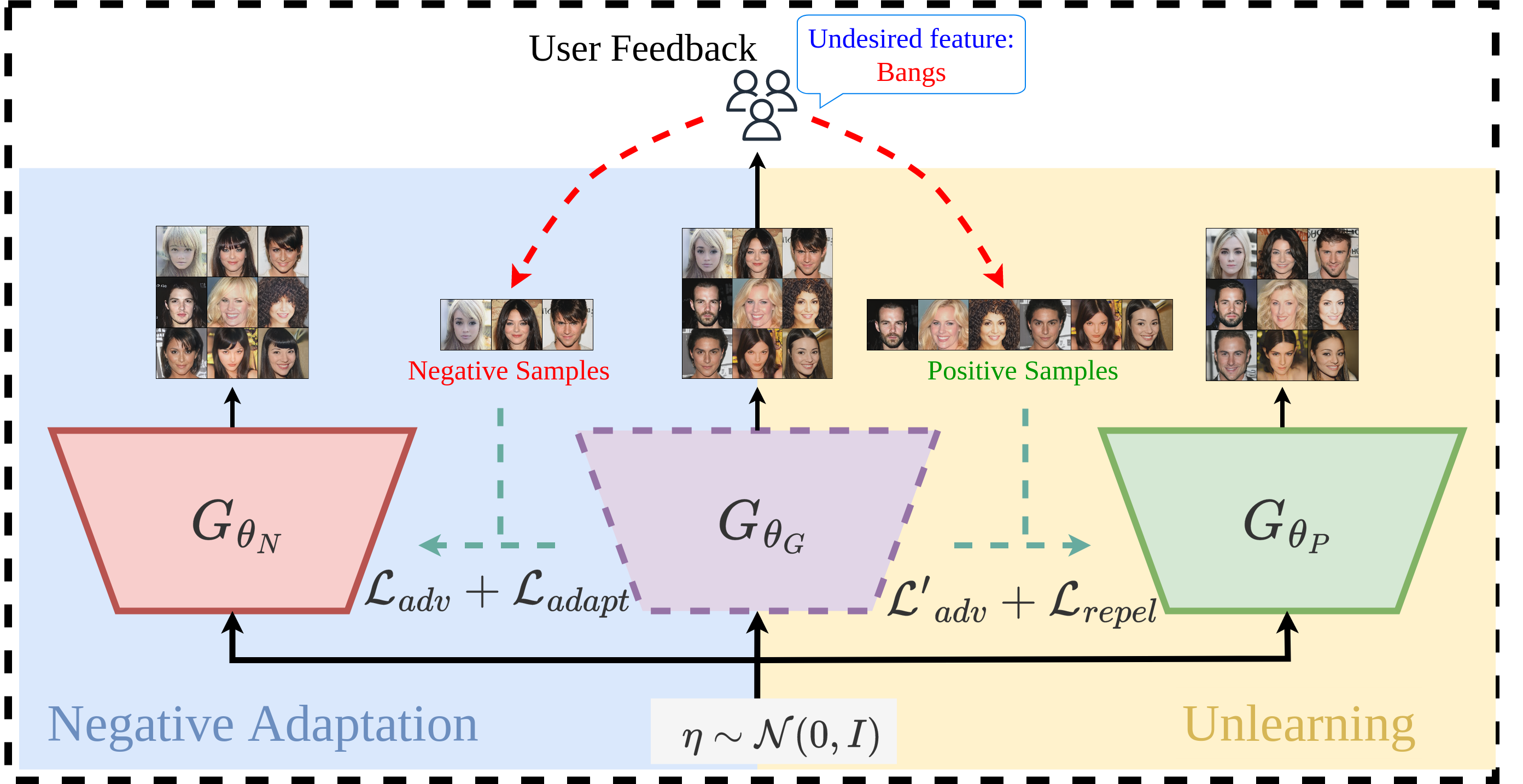
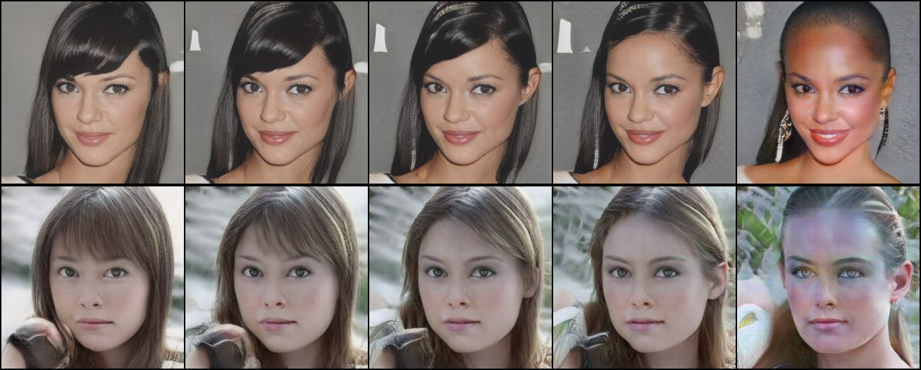
The core idea behind the proposed method relies on the simple observation that there exist interpretable meaningful directions in the parameter space of the generator (Cherepkov et al., 2021). This observation is the main source of motivation for the proposed method. In particular, the first stage of the proposed method leads to parameters that generate only negative samples. While the parameters of the original pre-trained generator generate both positive as well as negative samples. Hence, the difference between the adapted generator’s parameter and the original generator’s parameter can be interpreted as the direction in parameter space that leads to a decrease in the generation of negative samples. Given this, it is sensible to move away from the original parameters in this direction to further reduce the generation of negative samples. This observation is shown in figure 1. However, such extrapolation doesn’t guarantee the preservation of the quality of the other features in the generated images (see last columns of figure 1) and lead to deterioration of the generation quality. Inspired by this observation, we propose to train the generator using adversarial loss while encouraging the generator parameters to be away from the adapted generator’s parameters. An overview of the proposed method is shown in figure 2.

We summarize our contribution as follows:

• We introduce a two-stage approach for machine unlearning in GANs, adhering to the feedback-based unlearning framework. In the first stage, our method adapts the pre-trained GAN to the negative samples. In the second stage, we train the GAN using a repulsion loss, ensuring that the generator’s parameters diverge from those of the adapted GAN in stage 1. This guarantees that the newly learned parameters generate samples without the undesired features and leads to unlearning.

• By design, our method can operate in practical few-shot settings where the user provides a very small amount of negative samples.

• The proposed method is thoroughly tested on multiple datasets, considering various types of unlearning scenarios such as class-level unlearning and feature-level unlearning. Throughout these tests, we empirically observe that the quality of the generated samples is not compromised.

2 Related Work

2.1 Machine Unlearning

The task of machine unlearning is to forget specific learned information or to erase the influence of a particular subset of training data from a trained model. This can be naively done by removing the unwanted data subset from the training dataset and then retraining the model from scratch. However, retraining is computationally costly and becomes impossible if the unlearning request comes recursively for single data points. The task of recursively ’unlearning’ i.e. removing information of a single data point in an online manner (also known as decremental learning) for the SVM algorithm was introduced in  (Cauwenberghs & Poggio, 2000). However, when multiple data points are added or removed, these algorithms become slow because they need to be applied to each data point individually. So (Karasuyama & Takeuchi, 2009) introduced a newer type of SVM training algorithm that can efficiently update an SVM model when multiple data points are added or removed simultaneously. Later, inspired by the problem of protecting user privacy  (Cao & Yang, 2015) developed efficient ways to delete data from certain statistical query algorithms and coined the term “machine unlearning”. However, their methods can only be used for very structured problems and are not applicable to complex machine-learning algorithms such as k-means algorithms proposed in  (Ginart et al., 2019) nor in random forests algorithms  (Brophy & Lowd, 2021). (Ginart et al., 2019) gave an efficient deletion algorithm for the k-means clustering problem and gave the first definition of effective data deletion that can apply to randomized algorithms, in terms of statistical indistinguishability. Depending upon this statistical indistinguishability criteria machine unlearning processes are widely classified into exact unlearning  (Ginart et al., 2019; Brophy & Lowd, 2021) and approximate unlearning methods  (Neel et al., 2021; Nguyen et al., 2020). The goal of exact unlearning is to completely eliminate the influence of unwanted data from the learned model. In this case, the parameter distributions of the unlearned model and the retrained model should match exactly in terms of probability. On the other hand, in approximate unlearning, the influence of data is removed partially i.e. the distributions of the unlearned and retrained model’s parameters are close to some small multiplicative and additive terms  (Neel et al., 2021). To remove the influence of unwanted data  (Wu et al., 2020a) proposed parameter perturbation technique using the gradients cached during the training process. Even though it is faster in terms of computational time but quite memory intensive due to the storage of cached gradients. To reduce this issue (Guo et al., 2020; Graves et al., 2021) proposed to remove the influence using the method of influence function  (Koh & Liang, 2017). However, these methods are computationally expensive due to the Hessian inversion techniques and are only limited to small convex models. To extend the idea of influence removal of unwanted data in non-convex models such as deep neural networks  (Golatkar et al., 2020b) proposed a scrubbing mechanism in deep networks in a classification setting. Inspired by the same motivation of unlearning in classification models  (Tanno et al., 2022) proposed a mechanism based on variational-bayesian approach (Nguyen et al., 2020). Even though all of these methods achieve unlearning but fail to generalize to a setting where the underlying datasets are inaccessible. All these methods require full or partial access to the training dataset and even sometimes test dataset Tanno et al. (2022). To solve this problem  (Chundawat1 et al., 2023) extended classifier unlearning in a zero-shot environment where dataset access is not required. However, it is unknown how these techniques could be applied to unsupervised models such as state-of-the-art generative models. So, this work proposes to fill this gap by unlearning undesired features produced from a pre-trained GAN in a zero-shot setting.

2.2 Few-Shot Generative Domain Adaptation

The area of few-shot generative domain adaptation deals with the problem where a pre-trained generative model is adapted to a target domain using very few samples. A general strategy to do this is to fine-tune the model on target data using appropriate regularizers. Eg. Wang et al. (2018) observed that using a single pre-trained GAN for fine-tuning is good enough for adaptation. However, due to the limited amount of target data, this could lead to mode collapse, hence Noguchi & Harada (2019) proposed to fine-tune only the batch statistics of the model. Hence, they only fine-tune the scale and shift parameters of normalization layers for adaptation. Although, such a strategy can be very restrictive in practice. To overcome this issue, Wang et al. (2020) proposed to append a ‘miner’ network before the generator. In particular, they propose a two-stage framework, where the miner network is first trained to appropriately transform the input latent space to capture the target domain distribution then the whole pipeline is re-trained using target data. While these fine-tuning based methods give equal weightage to all the parameters of the generator, Li et al. (2020) proposed to fine-tune the parameter using Elastic Weight Consolidation (EWC). In particular, EWC is used to penalize large changes in important parameters. This importance is quantified using fischer-information while adapting the pre-trained GAN. Mo et al. (2020) showed that fine-tuning a GAN by freezing the lower layers of discriminator is also good enough in few-shot setting. Recently, a string of work (Ojha et al., 2021; Xiao et al., 2022; Lee et al., 2021) focuses on few-shot adaptation by preserving the cross-domain correspondence. Lastly,  Mondal et al. (2022) suggested an inference-time optimization approach where a they prepend a latent-learner, and the latent-learner is optimized every time a new set of images are to be generated from target domain.

As mentioned earlier, our approach involves an adaptation stage, where we adapt the pre-trained GAN to the negative samples provided by the user. In practive, the amount of negative samples provided by the user is very less hence such an adaptation falls under the category of few-shot generative domain adaptation. Hence, we make use of EWC (Li et al., 2020) for this adaptation phase (cf. Section 3.2 for details).

3 Proposed Methodology

3.1 Problem Formutation and Method Overview

Consider the generator $G_{\theta_{G}}$ of a pre-trained GAN with parameters $\theta_{G}$. The GAN is trained using a dataset ${\mathcal{D}}=\{{\mathbf{x}}_{i}\}_{i=1}^{|{\mathcal{D}}|}$, where ${\mathbf{x}}_{i}\overset{iid}{\sim}p_{X}(x)$. Using the feedback-based framework (Moon et al., 2023), we obtain a few negative and positive samples, marked by the user. Specifically, the user is provided with $n$ samples ${\mathcal{S}}=\{{\mathbf{y}}_{i}\}_{i=1}^{n}$ where ${\mathbf{y}}_{i}$ are the generated samples from the pre-trained GAN. The user identifies a subset of these samples ${\mathcal{S}}_{n}=\{{\mathbf{y}}_{i}\}_{i\in s_{n}}$, as negative samples or samples with undesired features, and the rest of the samples ${\mathcal{S}}_{p}=\{{\mathbf{y}}_{i}\}_{i\in s_{p}}$ as positive samples or samples that don’t possess the undesired features. Here, $s_{p}$ and $s_{n}$ are index sets such that $s_{p}\cup s_{n}=\{1,2,\ldots,n\}$ and $s_{p}\cap s_{n}=\phi$. Given this, the goal of unlearning is to learn the parameters $\theta_{P}$ such that the generator $G_{\theta_{P}}$ generates only positive samples. In other words, the parameters $\theta_{P}$ should lead to unlearning of the undesired features.

In this work, we adopt a two-stage approach for unlearning the undesired features. In Stage 1, we adapt the pre-trained generator $G_{\theta_{G}}$ on the negative samples. This step gives us the parameters $\theta_{N}$ such that $G_{\theta_{N}}$ generates only negative samples. In Stage 2, we actually unlearn the undesired feature by training the original generator $G_{\theta_{G}}$ on positive samples using the usual adversarial loss while adding an additional regularization term that makes sure that the learned parameter is far from $\theta_{N}$. We call this regularization term repulsion loss as it repels the learned parameters from $\theta_{N}$. We describe each of these stages in detail in subsequent sections.

3.2 Stage-1: Negative Adaptation

Inspired by (Tanno et al., 2022), the first stage involves adapting the pre-trained generator $G_{\theta_{G}}$ on the negative samples, ${\mathcal{S}}_{n}$ that are obtained through feedback from the user. The aim here is to obtain parameter $\theta_{N}$ such that the generator $G_{\theta_{N}}$ only generates samples that possess the undesired feature.

However, one thing to note here is that the number of negative samples marked by the user ($|{\mathcal{S}}_{n}|$) might be much less in number (of the order of a few hundreds). Directly adapting a pre-trained GAN with a much smaller amount of samples could lead to catastrophic forgetting (McClelland et al., 1995; McCloskey & Cohen, 1989). Thankfully, there is a rich literature on few-shot generative domain adaptation available. See Section 2.2 for a discussion on few-shot generative adaptation. Here, we use one of the simplest methods, namely, Elastic Weight Consolidation (EWC) based adaptation (Li et al., 2020), mainly because of its simplicity and ease of implementation. EWC-based adaptation relies on the simple observation that the ‘rate of change’ of weights is different for different layers; i.e., different layers need to be regularized differently. Further, this ‘rate of change’ is observed to be inversely proportional to the fisher information, $F$ of the corresponding weights. As a consequence, the fisher information can be used for penalizing changes in weights in different layers.

In our context, we want to adapt the pre-trained GAN on the negative samples. Hence, the optimal parameter $\theta_{N}$ for the adapted GAN can be obtained by solving the following optimization problem:

$$\theta_{N},\phi_{N}=\arg\underset{\theta}{\min}~{}\underset{\phi}{\max}~{}{\mathcal{L}}_{adv}+\gamma\mathcal{L}_{adapt}$$ (1)

where,

$${\mathcal{L}}_{adv}=\underset{{\mathbf{x}}\sim p_{{\mathcal{S}}_{n}}(x)}{\mathbb{E}}\left[\log D_{\phi}({\mathbf{x}})\right]+\underset{{\mathbf{z}}\sim p_{Z}(z)}{\mathbb{E}}\left[\log(1-D_{\phi}(G_{\theta}({\mathbf{z}})))\right]$$ (2)

$$\mathcal{L}_{adapt}=\lambda\sum_{i}F_{i}(\theta_{i}-\theta_{G,i})$$ (3)

$$F=\mathbb{E}\left[-\frac{\partial^{2}}{\partial\theta_{G}^{2}}{\mathcal{L}}({\mathcal{S}}_{n}\mid\theta_{G})\right]$$ (4)

Here, $p_{Z}(z)$ is the standard Gaussian, $p_{{\mathcal{S}}_{n}}(x)$ is the induced distribution due to ${\mathcal{S}}_{n}$ and ${\mathcal{L}}({\mathcal{S}}_{n}\mid\theta_{G})$ is the log-likelihood which is calculated through binary cross-entropy loss using the output of the discriminator as mentioned in Li et al. (2020). In practice, we train multiple instances of the generator to obtain multiple $\theta_{N}$. Specifically, given the negative samples ${\mathcal{S}}_{n}$, we adapt the pre-trained GAN $k$ times to obtain $\{\theta_{N}^{j}\}_{j=1}^{k}$.

3.3 Stage-2: Unlearning

During second stage of our method, the actual unlearning of undesired features takes place. In particular, this stage is motivated by the observation that there exist meaningful directions in the parameter space of the generator. This is shown in Fig. 2. However, such extrapolation-based schemes could lead to degradation in the quality of generated images.

Nevertheless, the above observation indicates that traversing away from $\theta_{N}$ helps us to erase or unlearn the undesired features. Therefore, a logical question to ask is can we transverse in the parameter space of a generator in such a way the parameters remain far from $\theta_{N}$ while making sure that the quality of generated samples doesn’t degrade? To solve this problem, we make use of the positive samples ${\mathcal{S}}_{p}$ provided by the user. Particularly, we propose to re-train the given GAN on the positive samples while incorporating a repulsion loss component that ‘repulsions’ or keeps the learned parameters away from $\theta_{N}$. Mathematically, we obtain the parameters after unlearning $\theta_{P},\phi_{P}$ by solving the following optimization problem:

$$\theta_{P},\phi_{P} =\arg\underset{\theta}{\min}~{}\underset{\phi}{\max}~{}{\mathcal{L}}_{adv}^{{}^{\prime}}+\gamma\mathcal{L}_{repulsion}$$ (5)

$$\text{where,}~{}~{}~{}{\mathcal{L}}_{adv}^{{}^{\prime}} =\underset{{\mathbf{x}}\sim p_{{\mathcal{S}}_{p}}(x)}{\mathbb{E}}\left[\log D_{\phi}({\mathbf{x}})\right]+\underset{{\mathbf{z}}\sim p_{Z}(z)}{\mathbb{E}}\left[\log(1-D_{\phi}(G_{\theta}({\mathbf{z}})))\right]$$ (6)

Here, $p_{{\mathcal{S}}_{p}}(x)$ is the distribution induced by positive samples ${\mathcal{S}}_{p}$, and $\mathcal{L}_{repulsion}$ is the repulsion loss. The repulsion loss is chosen such that it encourages the learned parameters to be far from $\theta_{N}$ obtained from Stage-1. Further, $\mathcal{L}^{\prime}_{adv}$ encourages the parameters to capture the desired distribution $p_{{\mathcal{S}}_{p}}(x)$. Hence, the combination of these two terms makes sure that we transverse in the parameter space maintaining the quality of generated samples while unlearning the undesired features as well.

3.4 Choice of Repulsion Loss

As mentioned above, the repulsion loss should encourage the learned parameter to traverse away from $\theta_{N}$ obtained from the negative adaptation stage. There is a lineage of research work in Bayesian learning called Deep Ensembles, where multiple MAP estimates of a network are used to approximate full-data posterior (Levin et al., 1990; Hansen & Salamon, 1990; Breiman, 1996; Lakshminarayanan et al., 2017; Ovadia et al., 2019; Wilson & Izmailov, 2020; D’Angelo & Fortuin, 2021a). The main issue faced in this area is that of diversity of the members in the ensembles. In other words, if the members of an ensemble are not diverse enough, then the posterior approximation might not capture the multi-modal nature of full-data posterior. As a consequence, there are several methods proposed to increase the diversity of the members of the ensemble (Huang et al., 2016; Von Oswald et al., 2020; D’Angelo & Fortuin, 2021b; Wenzel et al., 2020; D’Angelo & Fortuin, 2021a). Inspired by these developments, we make use of the technique proposed in D’Angelo & Fortuin (2021a) where the members of an ensemble interact with each other through a repulsive force that encourages diversity in the ensemble. Particularly, we explore three choices for repulsion loss:

$${\mathcal{L}}_{repulsion}^{\text{IL2}}=\frac{1}{||\theta-\theta_{N}||_{2}^{2}},\hskip 11.38109pt{\mathcal{L}}_{repulsion}^{\text{NL2}}=-||\theta-\theta_{N}||_{2}^{2},\hskip 11.38109pt{\mathcal{L}}_{repulsion}^{\text{El2}}=\exp(-\alpha||\theta-\theta_{N}||_{2}^{2})$$ (7)

where, ${\mathcal{L}}_{repulsion}^{\text{IL2}}$, ${\mathcal{L}}_{repulsion}^{\text{NL2}}$ and ${\mathcal{L}}_{repulsion}^{\text{El2}}$ are the inverse $\ell 2$, negative $\ell 2$ and exponential negative $\ell 2$ loss between $\theta$ and $\theta_{N}$. It can be seen that minimization of all of these choices will force $\theta$ to be away from $\theta_{N}$, consequently surving our purpose.

Algorithm 1 Negative Adaptation

Required: Pre-trained parameters ($\theta_{G}$, $\phi_{D}$), Negative samples (${\mathcal{S}}_{n}$), Number of adapted models ($k$)

  Initialize: $j\leftarrow 0$

  while $j\leq k$ do

     $\theta\leftarrow\theta_{G}$, $\phi\leftarrow\phi_{D}$

     repeat

        Sample ${\mathbf{x}}\sim{\mathcal{S}}_{n}$ and ${\mathbf{z}}\sim{\mathcal{N}}(0,I)$

        ${\mathcal{L}}_{adv}\leftarrow$

        $\log{D_{\phi}({\mathbf{x}})}+\log{(1-D_{\phi}(G_{\theta}({\mathbf{z}})))}$

        ${\mathcal{L}}_{adapt}\leftarrow\lambda\sum_{i}F_{i}(\theta_{i}-\theta_{G,i})$

         $\theta\leftarrow\theta-\eta\nabla_{\theta}({\mathcal{L}}_{adv}+{\mathcal{L}}_{adapt})$

     until convergence

     $\theta_{N}^{j}\leftarrow\theta$

  end while

Algorithm 2 Unlearning

Required: Pre-trained parameters ($\theta_{G}$, $\phi_{D}$), Positive samples (${\mathcal{S}}_{p}$), Adapted models ($\theta_{N}=\{\theta_{N}^{j}\}_{j=1}^{k}$)

  Initialize: $\theta_{P}\leftarrow\theta_{G}$, $\phi_{P}\leftarrow\phi_{D}$

  repeat

     Sample ${\mathbf{x}}\sim{\mathcal{S}}_{p}$ and ${\mathbf{z}}\sim{\mathcal{N}}(0,I)$

     ${\mathcal{L}}^{{}^{\prime}}_{adv}\leftarrow$

     $\log{D_{\phi}({\mathbf{x}})}+\log{(1-D_{\phi}(G_{\theta}({\mathbf{z}})))}$

     Choose ${\mathcal{L}}_{repulsion}$ from Eq. 7

      $\theta\leftarrow\theta-\eta\nabla_{\theta}({\mathcal{L}}_{adv}+{\mathcal{L}}_{repulsion})$

  until convergence

4 Experiments and Results

4.1 Dataset

In the following section we demonstrate the results pertaining to our method both qualitatively as well as quantitatively. As discussed earlier, in unlearning, we want the generator of the GAN to ‘forget’ a particular feature. In other words, after unlearning, the generator should not generate images containing the undesired (or unlearnt) feature. As discussed earlier, we look at two type of unlearning settings: (i) Class-level unlearning and (ii) Feature-level unlearning. We use MNIST dataset (LeCun et al., 1998) for class-level unlearning. It consists of $60,000$ $28\times 28$ dimensional black and white images of handwritten digits. For our purpose, we take three digit classes: 1, 4, and 8 for unlearning. Similarly, we use CelebA-HQ dataset (Liu et al., 2015) for feature-level unlearning. CelebA-HQ contains $30,000$ RGB high-quality celebrity face images of dimension $256\times 256$. Here, we unlearn the following subtle features: (a) Bangs, (b) Hats, (c) Bald, and (d) Eyeglasses.

4.2 Experimental Details

Training Details: We use one of the state-of-the-art and widely used StyleGAN2 (Karras et al., 2020) for demonstrating the performance of the proposed method on the tasks mentioned in pervious section. The StyleGAN is trained on entire MNIST and CelebA-HQ to obtain the pre-trained GAN from which specific features are to be unlearnt. The FID of samples generated by pre-trained GAN for MNIST is $5.4$ whereas the FID is $5.3$. The training details of StyleGAN are given in Appendix Section A.1.1.

Unlearning Details: As mentioned earlier, we operate under the feedback-based framework. To obtain the feedback, we employ a pre-trained classifier. Specifically, we pre-train the classifier to classify a given image as desired or undesired (depending upon the feature under consideration). We classify 5000 generated images from pre-trained GAN as positive and negative samples using the pre-trained classifier. The generated samples containing the undesired features are marked as negative samples and rest of the images are marked as positive samples. These samples are then used in Stage-1 and Stage-2 of the proposed method for unlearning as described in Section 3. We evaluate our result using all the choices of repulsion loss as mentioned in Eq. 7. For reproducibility, we have provided all the hyper-parameters and details in the Appendix Section A.1.2 and A.1.3.

4.3 Baselines and Evaluation Metrics

Baselines: To the best of our knowledge, ours is the first work that addresses the problem of unlearning in high-fidelity generator models such as StyleGAN. Hence, we evaluate and compare our method with all the candidates for repulsion loss presented in Eq. 7. Further, we also include the results with extrapolation in the parameter space as demonstrated in figure 1. We evaluate the performance of each method across three independent runs and report the result in the form of mean $\pm$ std. dev.

Evaluation Metrics: Various metrics have been devised for assessing machine unlearning methods (Xu et al., 2020). To gauge the effectiveness of our proposed techniques and the baseline methods, we utilize three fundamental evaluation metrics:

1. Percentage of Un-Learning (PUL): This metric quantifies the extent of unlearning by measuring the reduction in the number of negative samples generated by the GAN post-unlearning compared to the pre-unlearning state. PUL is computed as:

   $$\text{PUL}=\frac{(S_{n})_{\theta_{G}}-(S_{n})_{\theta_{P}}}{(S_{n})_{\theta_{G}}}\times 100$$ (8)

   where, $(S_{n})_{\theta_{G}}$ and $(S_{n})_{\theta_{P}}$ represent the number of negative samples generated by the original GAN and the GAN after unlearning respectively. We generate 15,000 random samples from both GANs and employ a pre-trained classifier (as detailed in Section 4.2) to identify the negative samples. PUL provides a quantitative measure of the extent of the unlearning algorithm in eliminating the undesired feature from the GAN.

2. Fréchet Inception Distance (FID): While PUL quantifies the degree of unlearning, it does not assess the quality of samples generated by the GAN post-unlearning. Hence, we calculate the FID (Heusel et al., 2017) between the generated samples and the original dataset. For correctness, samples containing undesired features are removed from the original dataset, as the unlearning process aims to generate samples from the data distribution after removing undesired features.

3. Retraining FID (Ret-FID): Ultimately, the ideal objective of unlearning is to produce a model as if it were trained on data entirely devoid of undesired features. To illustrate this facet of unlearning, we compute the FID between the outputs of the GAN after unlearning and the GAN trained from scratch on the dataset obtained after eliminating undesired features.

Please note that the original dataset is unavailable during the unlearning process. Consequently, the use of the original dataset is solely for evaluation purposes.

4.4 Unlearning Results

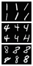
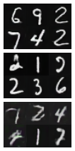
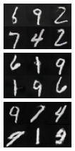
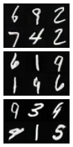
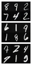
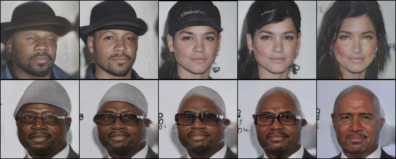
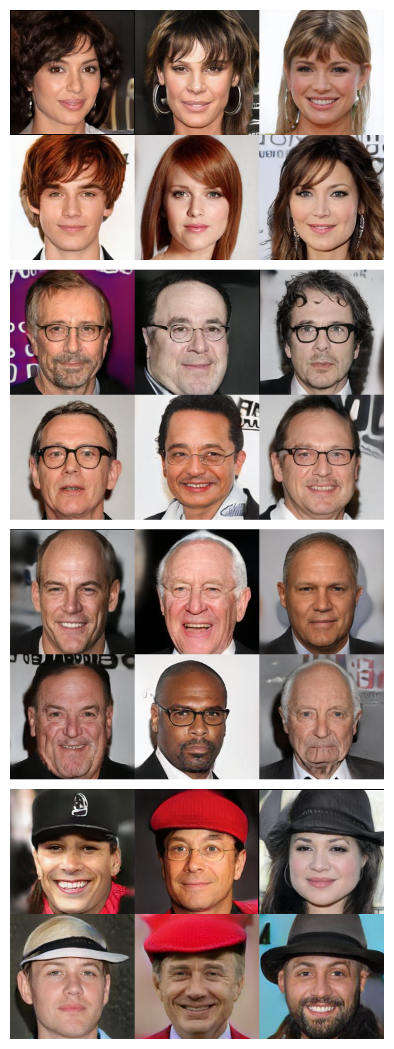
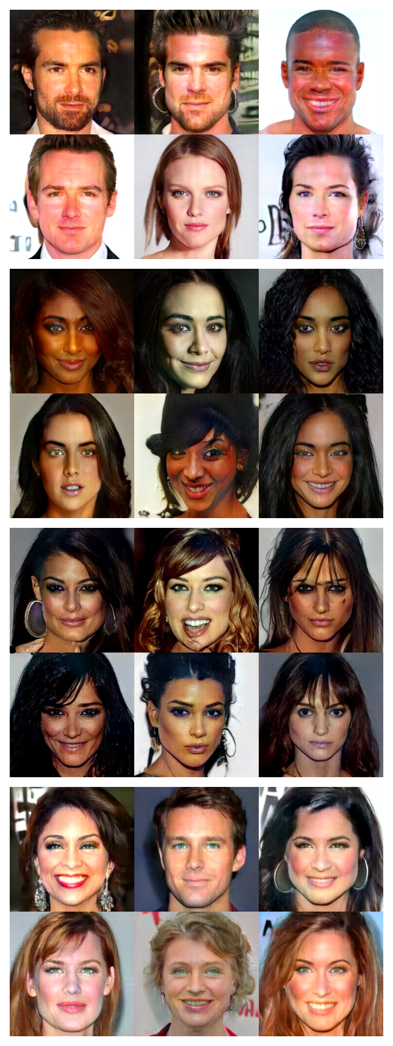
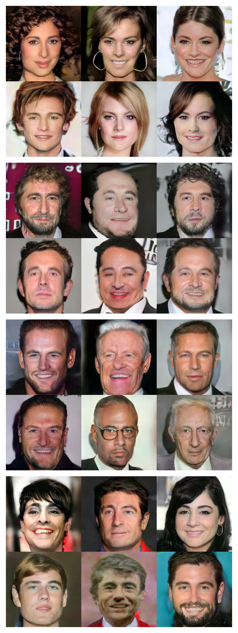
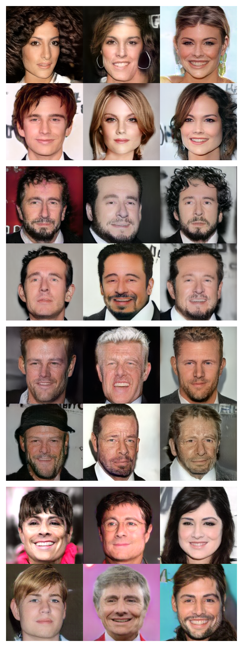
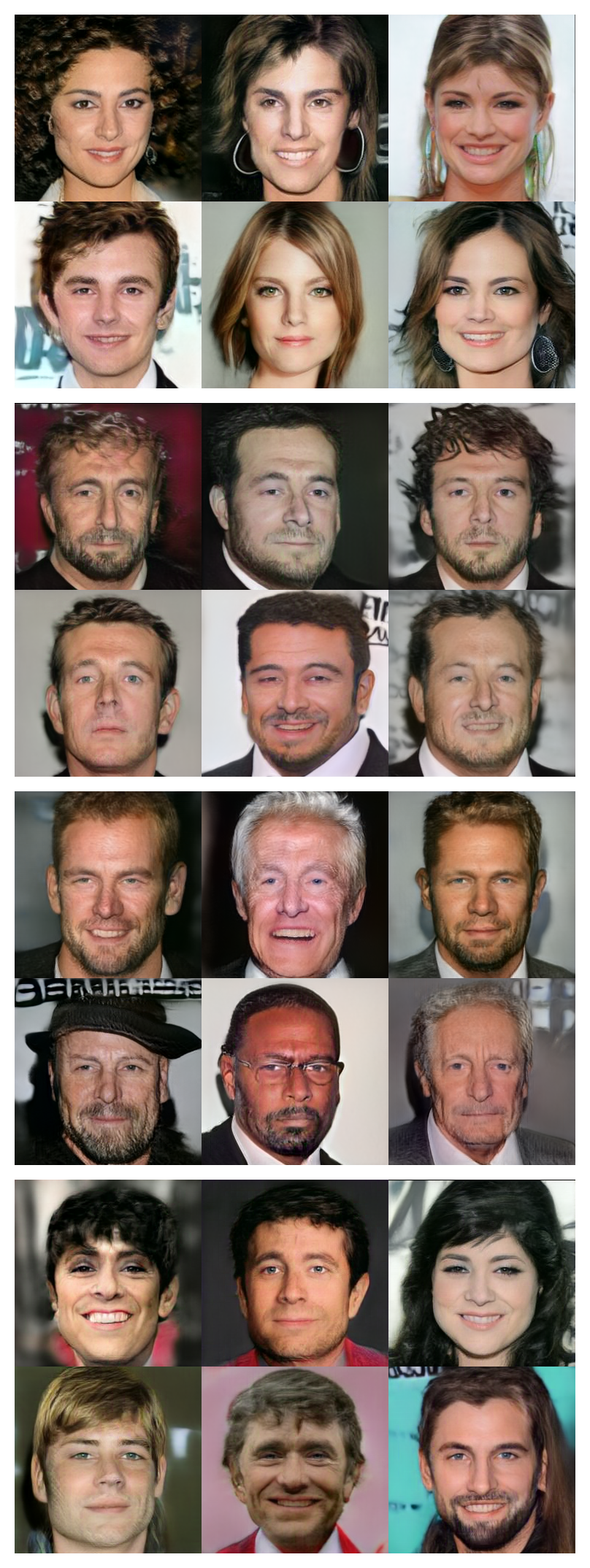
We present our results and observations on MNIST and CelebA-HQ in Table 2 and 2 respectively. We observe that the choice of ${\mathcal{L}}_{repulsion}^{\text{EL2}}$ as repulsion loss provides highest PUL in most of the cases for both the dataset. Further, it also provides best FID and Ret-FID as compared to other choices of repulsion loss. ${\mathcal{L}}_{repulsion}^{\text{NL2}}$ is stands out to be the second best in these metrics for most of the cases. For MNIST, we observe in Table 2 that the proposed method with ${\mathcal{L}}_{repulsion}^{\text{EL2}}$ as repulsion loss consistently provides a PUL of above $95\%$ while giving the best FID and Ret-FID compared to other methods. We also observe that Extrapolation in parameter space leads to significant PUL albeit the FID and Ret-FID are considerably worse compared to proposed method under different repulsion loss. This shows that the proposed method is decently solves the task of unlearning at class-level. Next, feature-level unlearning results on CelebA-HQ are presented in Table 2. It can be seen that the proposed method with ${\mathcal{L}}_{repulsion}^{\text{EL2}}$ as repulsion loss consistently provides a PUL of above $90\%$, illustrating significant unlearning of undesired features. Further, the FID and Ret-FID using ${\mathcal{L}}_{repulsion}^{\text{EL2}}$ stand out to be the best among all the methods. Furthermore, we observe that the FID of the samples generated by the unlearnt GAN (on Hats) using ${\mathcal{L}}_{repulsion}^{\text{EL2}}$ drops by about $4.15$ points while it drops by $4.3$ and $6.01$ points while using ${\mathcal{L}}_{repulsion}^{\text{NL2}}$ and ${\mathcal{L}}_{repulsion}^{\text{IL2}}$ as compared to the pre-trained GAN. This demonstrates that the proposed method is able to unlearn the undesired feature (hats) by compromising slightly on the quality of generated samples. On the other hand, we notice that Extrapolation in parameter space provides decent PUL, however, it can be seen that the FID and Ret-FID scores are much worse. This supports our claim that extrapolation might unlearn the undesired feature, however, it deteriorates the quality of generated samples significantly. The visual illustration of these methods is shown in figure 3. Here, we observe that the proposed method effectively unlearns the undesired feature. Moreover, it can be seen that the unlearning through extrapolation leads to unlearning of correlated features as well. E.g. Bangs are correlated with female attribute. It can be seen that the unlearning of Bangs through extrapolation also leads to unlearning of female feature which is not desired. However, while unlearning through the proposed method unlearns Bangs only, while keeping the other features as it is. Similar visual results for MNIST is provided in Appendix in Section A.2.

Table 1: PUL ($\uparrow$), FID ($\downarrow$) and Ret-FID ($\downarrow$) after unlearning MNIST classes. FID of pre-trained GAN: $5.4$.

Features	Metrics	Extrapolation	${\mathcal{L}}_{repulsion}^{\text{NL2}}$	${\mathcal{L}}_{repulsion}^{\text{IL2}}$	${\mathcal{L}}_{repulsion}^{\text{EL2}}$
Class-1	PUL	95.10 $\pm$ 0.69	97.85 $\pm$ 2.25	92.97 $\pm$ 0.48	99.32 $\pm$ 0.43
	FID	41.39 $\pm$ 1.76	9.69 $\pm$ 0.07	13.06 $\pm$ 0.46	9.65 $\pm$ 0.21
	Ret-FID	42.98 $\pm$ 0.68	6.70 $\pm$ 0.25	16.55 $\pm$ 0.54	6.29 $\pm$ 0.18
Class-4	PUL	94.50 $\pm$ 0.05	93.03 $\pm$ 0.7	90.39 $\pm$ 1.36	96.23 $\pm$ 0.54
	FID	17.90 $\pm$ 0.35	10.50 $\pm$ 0.34	15.54 $\pm$ 0.05	10.24 $\pm$ 0.19
	Ret-FID	27.81 $\pm$ 0.37	6.26 $\pm$ 0.12	8.64 $\pm$ 0.9	5.80 $\pm$ 0.04
Class-8	PUL	90.90 $\pm$ 0.12	97.92 $\pm$ 0.677	98.28 $\pm$ 0.55	95.22 $\pm$ 0.34
	FID	45.79 $\pm$ 0.29	9.95 $\pm$ 0.177	9.72 $\pm$ 0.31	8.89 $\pm$ 0.52
	Ret-FID	44.3 $\pm$ 0.40	6.70 $\pm$ 0.18	11.64 $\pm$ 0.46	5.68 $\pm$ 0.10

Table 2: PUL ($\uparrow$), FID ($\downarrow$) and Ret-FID ($\downarrow$) after unlearning CelebA-HQ features. FID of pre-trained GAN: $5.3$.

Features	Metrics	Extrapolation	${\mathcal{L}}_{repulsion}^{\text{NL2}}$	${\mathcal{L}}_{repulsion}^{\text{IL2}}$	${\mathcal{L}}_{repulsion}^{\text{EL2}}$
Bangs	PUL	89.54 $\pm$ 0.09	90.41 $\pm$ 0.19	84.05 $\pm$ 1.03	90.45 $\pm$ 1.02
	FID	11.54 $\pm$ 0.07	11.92 $\pm$ 0.46	13.09 $\pm$ 0.10	11.16 $\pm$ 0.08
	Ret-FID	11.02 $\pm$ 0.06	08.69 $\pm$ 0.05	09.07 $\pm$ 0.18	07.94 $\pm$ 0.32
Hat	PUL	94.35 $\pm$ 0.12	93.99 $\pm$ 1.70	94.00 $\pm$ 0.75	94.40 $\pm$ 2.19
	FID	12.18 $\pm$ 0.04	9.60 $\pm$ 0.25	11.31 $\pm$ 0.06	9.45 $\pm$ 0.96
	Ret-FID	10.12 $\pm$ 0.07	06.44 $\pm$ 0.11	07.25 $\pm$ 0.13	06.31 $\pm$ 0.64
Bald	PUL	94.44 $\pm$ 0.34	97.13 $\pm$ 1.42	83.51 $\pm$ 2.18	93.97 $\pm$ 2.65
	FID	23.44 $\pm$ 0.02	14.7 $\pm$ 0.55	12.94 $\pm$ 0.89	11.07 $\pm$ 0.86
	Ret-FID	26.40 $\pm$ 0.30	09.03 $\pm$ 0.13	09.87 $\pm$ 0.04	07.83 $\pm$0.05
Eyeglasses	PUL	92.80 $\pm$ 0.14	83.76 $\pm$ 3.21	75.23 $\pm$ 6.25	93.63 $\pm$ 0.42
	FID	23.70 $\pm$ 0.07	12.81 $\pm$ 0.88	13.12 $\pm$ 0.78	9.66 $\pm$ 0.58
	Ret-FID	19.10 $\pm$ 0.10	07.93 $\pm$ 0.99	06.11 $\pm$ 0.24	09.84$\pm$0.23

Table 3: Effect on PUL ($\uparrow$) and FID ($\downarrow$) with and without repulsion loss.

Features	Metrics	${\mathcal{L}}_{adv}^{{}^{\prime}}$	${\mathcal{L}}_{adv}^{{}^{\prime}}+{\mathcal{L}}_{repulsion}^{\text{EL2}}$
Bangs	PUL	79.89 $\pm$ 0.49	90.45 $\pm$ 1.01
	FID	10.50 $\pm$ 0.24	11.16 $\pm$ 0.08
Hat	PUL	84.68 $\pm$ 3.89	94.40 $\pm$ 2.19
	FID	9.66 $\pm$ 0.16	9.45 $\pm$ 0.96

(a) Original samples

(b) Extrapolation

(c) ${\mathcal{L}}_{repulsion}^{\text{IL2}}$

(d) ${\mathcal{L}}_{repulsion}^{\text{NL2}}$

(e) ${\mathcal{L}}_{repulsion}^{\text{EL2}}$

Figure 3: Results of Unlearning undesired feature via different methods. The undesired features contain Bangs (top row), Eyeglasses (second row), Bald head (third row), Hat (bottom row)

4.5 Ablation Study

Lastly, we present the ablation study to observe the effect of repulsion loss. In particular, we see if adapting the pre-trained GAN only on the positive samples leads to desired levels of unlearning. Our observations on CelebA-HQ for Bangs and Hats are presented in Table 3. Here, we use ${\mathcal{L}}_{repulsion}^{\text{EL2}}$ as repulsion loss. It can be seen that only using adversarial loss doesn’t lead to significant unlearning of undesired feature. E.g. using repulsion loss provides and increase of about $10.56\%$ and $9.72\%$ in PUL. The FID increases by minor $0.66$ point on Bangs while it decreases by $0.21$ points on Hats. Hence, we conclude that repulsion loss is indeed crucial for unlearning.

5 Conclusion

In this work, we present a methodology to prevent the generation of samples containing undesired features from a pre-trained GAN. It is worth mentioning that our method does not assume the availability of the training dataset of the pre-trained GAN so it can generalize to zero-shot settings. In spite of these advantages, there are some limitations that our methodology can’t encompass such as changes in correlated features while unlearning undesired features. Due to high entanglement between the semantics features this kind of impact on other features is visible in the generated outputs. Despite these limitations, we believe that our work is an important step towards unlearning in deep generative models that cater to the widespread societal concerns of biased, racial, and harmful content creation from these models.

Appendix A Appendix

A.1 Training Details

Here, we provide the details pertaining to the proposed method. Specifically, we provide the details of the pre-trained GANs and pre-trained Classifiers used in the proposed method. We also provide details pertaining to the training strategy used during Unlearning. All the experiments are performed on RTX-A6000 GPUs with 48GB memory.

A.1.1 Details of Pre-trained GAN

As mentioned in the main text, we use the famous StyleGAN2 architecture to obtain the pre-trained GAN. We use the open-source pytorch repository for implementation. We resize the MNIST images to $32\times 32$ and CelebA-HQ images to $256\times 256$ to fit in the StyleGAN2 architecture. The latent space dimension for MNIST and CelebA-HQ is consequently set to $128\times 1$ and $512\times 1$. We train the GAN using the non-saturating adversarial loss alongwith path-regularization for training (Goodfellow et al., 2014; Karras et al., 2020). We use default optimizers and hyper-parameter as provided in the code for training. We train the GAN for $2\times 10^{5}$ and $3.6\times 10^{5}$ epochs for MNIST and CelebA-HQ respectively.

A.1.2 Details of Pre-trained Classifiers

We use pre-trained classifiers to simulate the process of obtaining the feedback. More specifically, the feedbacks (positive and negative samples) are obtained by passing the generated samples (from the pre-trained GAN) through these pre-trained classifiers. The classifier classifies the generates samples into positive and negative samples. Furthermore, the classifiers are also employed for obtaining the evaluation metrics as discussed in Section 4.3 of the main text.

MNIST: We use simple LeNet model (LeCun et al., 1998) for classification among different digits of MNIST dataset. The model is trained with a batch-size of $256$ using Adam optimizer with a learning rate of $2\times 10^{-3}$, $\beta_{1}=0.9$ and $\beta_{2}=0.999$. The model is trained for a resolution of $32\times 32$ same as the pre-trained GAN for $12$ epochs. After training the classifier has an accuracy of $99.07\%$ on the test split of MNIST dataset.

CelebA-HQ: We use ResNext50 model (Xie et al., 2017) for classification among different facial attributes. Note that we train the classifier on normal CelebA as the ground truth values are available for it. The classifier is trained with a batch-size of $50$ usign Adamax optimizer with a learning rate of $2\times 10^{-3}$, $\beta_{1}=0.9$ and $\beta_{2}=0.999$. The model is trained for a resolution of $256\times 256$ for $3$ epochs. We also employ image augmentation techniques such as horizontal flip, image resize and cropping to improve the performance of the classifier. The trained model exhibits a test accuracy of $91.93\%$.

A.1.3 Unlearning Hyper-parameters

Here we mention the hyper-parameters pertaining to the proposed negative adaptation and unlearning stages. As mentioned, we use EWC regularizer during adaptation to avoid overfitting. The value of $\lambda$ (Eq. 3) is set to $5\times 10^{8}$ for all the experiments. Further, $\gamma$ (Eq. 1) is chosen between $0.1$, $1$ and $10$ when ${\mathcal{L}}_{repulsion}^{\text{IL2}}$ and ${\mathcal{L}}_{repulsion}^{\text{NL2}}$ are chosen as repulsion loss. It is varied between $10$ and $500$ when ${\mathcal{L}}_{repulsion}^{\text{EL2}}$ is chosen as repulsion loss. Further, the value of $\alpha$ for ${\mathcal{L}}_{repulsion}^{\text{EL2}}$ (Eq. 7) is varied between $0.1$ and $0.001$. These values are chosen and adjusted to ensure that both the loss components ${\mathcal{L}}_{adv}^{{}^{\prime}}$ and ${\mathcal{L}}_{repulsion}$ are minimized properly.

A.2 MNIST Qualitative Results

(a) Images generated from pre-trained GAN

(b) Unlearning via extrapolation

(c) Unlearning via reciprocal $\ell 2$ loss

(d) Unlearning via negative $\ell 2$ loss

(e) Unlearning via exponential $\ell 2$ loss

Figure 4: Results of Unlearning undesired feature via different methods. The undesired class contain class-1(top row), class-4(second row), class-8 (bottom row)

References

- Adegun et al. (2023) Adekanmi Adeyinka Adegun, Serestina Viriri, and Jules-Raymond Tapamo. Review of deep learning methods for remote sensing satellite images classification: experimental survey and comparative analysis. Journal of Big Data, 10(1):93, 2023.
- Arjovsky et al. (2017) TMartin Arjovsky, Soumith Chintala, and Léon Bottou. Wasserstein generative adversarial networks. In Proc. of ICML, 2017.
- Ball et al. (2017) John E Ball, Derek T Anderson, and Chee Seng Chan. Comprehensive survey of deep learning in remote sensing: theories, tools, and challenges for the community. Journal of applied remote sensing, 11(4):042609–042609, 2017.
- Breiman (1996) Leo Breiman. Bagging predictors. Machine learning, 24:123–140, 1996.
- Brophy & Lowd (2021) Jonathan Brophy and Daniel Lowd. Machine unlearning for random forests. In Proc. of ICML, 2021.
- Cao & Yang (2015) Yinzhi Cao and Junfeng Yang. Towards making systems forget with machine unlearning. In Proc. of IEEE Symposium on Security and Privacy, 2015.
- Cauwenberghs & Poggio (2000) Gert Cauwenberghs and Tomaso Poggio. Incremental and decremental support vector machine learning. In Proc. of NIPS, 2000.
- Celard et al. (2023) Pedro Celard, EL Iglesias, JM Sorribes-Fdez, Rubén Romero, A Seara Vieira, and L Borrajo. A survey on deep learning applied to medical images: from simple artificial neural networks to generative models. Neural Computing and Applications, 35(3):2291–2323, 2023.
- Cherepkov et al. (2021) Anton Cherepkov, Andrey Voynov, and Artem Babenko. Navigating the gan parameter space for semantic image editing. In Proceedings of the IEEE/CVF conference on computer vision and pattern recognition, pp. 3671–3680, 2021.
- Choudhary et al. (2022) Kamal Choudhary, Brian DeCost, Chi Chen, Anubhav Jain, Francesca Tavazza, Ryan Cohn, Cheol Woo Park, Alok Choudhary, Ankit Agrawal, Simon JL Billinge, et al. Recent advances and applications of deep learning methods in materials science. npj Computational Materials, 8(1):59, 2022.
- Chourasia & Shah (2023) Rishav Chourasia and Neil Shah. Forget unlearning: Towards true data-deletion in machine learning. In Proc. of ICML, 2023.
- Chundawat1 et al. (2023) Vikram S Chundawat1, Ayush K Tarun1, Murari Mandal, and Mohan Kankanhalli. Zero-shot machine unlearning. IEEE Transactions on Information Forensics and Security, 2023.
- D’Angelo & Fortuin (2021a) Francesco D’Angelo and Vincent Fortuin. Repulsive deep ensembles are bayesian. Advances in Neural Information Processing Systems, 34:3451–3465, 2021a.
- D’Angelo & Fortuin (2021b) Francesco D’Angelo and Vincent Fortuin. Repulsive deep ensembles are bayesian. Advances in Neural Information Processing Systems, 34:3451–3465, 2021b.
- Ginart et al. (2019) Antonio Ginart, Melody Guan, Gregory Valiant, and James Y. Zou. Making ai forget you: Data deletion in machine learning. In Proc. of NIPS, 2019.
- Golatkar et al. (2020a) Aditya Golatkar, Alessandro Achille, and Stefano Soatto. Forgetting outside the box: Scrubbing deep networks of information accessible from input-output observations. In Proc. of ECCV, 2020a.
- Golatkar et al. (2020b) Aditya Golatkar, Alessandro Achille, and Stefano Soatto. Eternal sunshine of the spotless net: Selective forgetting in deep networks. In Proc. of CVPR, 2020b.
- Golatkar et al. (2021) Aditya Golatkar, Alessandro Achille, Avinash Ravichandran, Marzia Polito, and Stefano Soatto. Mixed-privacy forgetting in deep networks. In Proc. of CVPR, 2021.
- Goldman (2020) E. Goldman. An introduction to the california consumer privacy act (ccpa). Santa Clara Univ. Legal Studies Research Paper, 2020.
- Goodfellow et al. (2014) Ian Goodfellow, Jean Pouget-Abadie, Mehdi Mirza, Bing Xu, David Warde-Farley, Sherjil Ozair, Aaron Courville, and Yoshua Bengio. Generative adversarial nets. In Proc. of NeuRIPS, 2014.
- Graves et al. (2021) Laura Graves, Vineel Nagisetty, and Vijay Ganesh. Amnesiac machine learning. In Proc. of AAAI, 2021.
- Guo et al. (2020) Chuan Guo, Tom Goldstein, Awni Hannun, and Laurens van der Maaten. Certified data removal from machine learning models. In Proc. of ICML, 2020.
- Hansen & Salamon (1990) Lars Kai Hansen and Peter Salamon. Neural network ensembles. IEEE transactions on pattern analysis and machine intelligence, 12(10):993–1001, 1990.
- Heusel et al. (2017) Martin Heusel, Hubert Ramsauer, Thomas Unterthiner, Bernhard Nessler, and Sepp Hochreiter. Gans trained by a two time-scale update rule converge to a local nash equilibrium. Advances in neural information processing systems, 30, 2017.
- Ho et al. (2020) Jonathan Ho, Ajay Jain, and Pieter Abbeel. Denoising diffusion probabilistic models. In Proc. of NeuRIPS, 2020.
- Huang et al. (2016) Gao Huang, Yixuan Li, Geoff Pleiss, Zhuang Liu, John E Hopcroft, and Kilian Q Weinberger. Snapshot ensembles: Train 1, get m for free. In International Conference on Learning Representations, 2016.
- Jia et al. (2021) Sen Jia, Shuguo Jiang, Zhijie Lin, Nanying Li, Meng Xu, and Shiqi Yu. A survey: Deep learning for hyperspectral image classification with few labeled samples. Neurocomputing, 448:179–204, 2021.
- Karasuyama & Takeuchi (2009) Masayuki Karasuyama and Ichiro Takeuchi. Multiple incremental decremental learning of support vector machines. In Proc. of NIPS, 2009.
- Karras et al. (2018a) Tero Karras, Timo Aila, and Samuli Laine. A style-based generator architecture for generative adversarial networks. In Proc. of CVPR, 2018a.
- Karras et al. (2018b) Tero Karras, Timo Aila, Samuli Laine, and Jaakko Lehtinen. Progressive growing of gans for improved quality, stability, and variation. In Proc. of ICLR, 2018b.
- Karras et al. (2020) Tero Karras, Samuli Laine, Miika Aittala, Janne Hellsten, Jaakko Lehtinen, and Timo Aila. Analyzing and improving the image quality of stylegan. In Proc. of CVPR, 2020.
- Karras et al. (2021) Tero Karras, Miika Aittala, Samuli Laine, Erik Härkönen, Janne Hellsten, Jaakko Lehtinen, and Timo Aila. Alias-free generative adversarial networks. Advances in Neural Information Processing Systems, 34:852–863, 2021.
- Koh & Liang (2017) Pang Wei Koh and Percy Liang. Understanding black-box predictions via influence functions. In Proc. of ICML, 2017.
- Lakshminarayanan et al. (2017) Balaji Lakshminarayanan, Alexander Pritzel, and Charles Blundell. Simple and scalable predictive uncertainty estimation using deep ensembles. Advances in neural information processing systems, 30, 2017.
- LeCun et al. (1998) Yann LeCun, Léon Bottou, Yoshua Bengio, and Patrick Haffner. Gradient-based learning applied to document recognition. Proceedings of the IEEE, 86(11):2278–2324, 1998.
- Lee et al. (2021) Hyuk-Gi Lee, Gi-Cheon Kang, Chang-Hoon Jeong, Han-Wool Sul, and Byoung-Tak Zhang. : Contrastive learning for cross-domain correspondence in few-shot image generation. In Proceedings of Workshop on Controllable Generative Modeling in Language and Vision (CtrlGen) at NeurIPS 2021, 2021.
- Levin et al. (1990) Esther Levin, Naftali Tishby, and Sara A Solla. A statistical approach to learning and generalization in layered neural networks. Proceedings of the IEEE, 78(10):1568–1574, 1990.
- Li et al. (2020) Yijun Li, Richard Zhang, Jingwan (Cynthia) Lu, and Eli Shechtman. Few-shot Image Generation with Elastic Weight Consolidation. In Proc. of NeurIPS, 2020.
- Liu et al. (2021) Zhichao Liu, Luhong Jin, Jincheng Chen, Qiuyu Fang, Sergey Ablameyko, Zhaozheng Yin, and Yingke Xu. A survey on applications of deep learning in microscopy image analysis. Computers in biology and medicine, 134:104523, 2021.
- Liu et al. (2015) Ziwei Liu, Ping Luo, Xiaogang Wang, and Xiaoou Tang. Deep learning face attributes in the wild. In Proceedings of International Conference on Computer Vision (ICCV), 2015.
- Ma et al. (2022) Zhuo Ma, Yang Liu, Ximeng Liu, Jian Liu, Jianfeng Ma, and Kui Ren. Learn to forget: Machine unlearning via neuron masking. In Proc. of IEEE Transactions on Dependable and Secure Computing, 2022.
- McClelland et al. (1995) James L McClelland, Bruce L McNaughton, and Randall C O’Reilly. Why there are complementary learning systems in the hippocampus and neocortex: insights from the successes and failures of connectionist models of learning and memory. Psychological review, 102, 1995.
- McCloskey & Cohen (1989) Michael McCloskey and Neal J Cohen. Catastrophic interference in connectionist networks: The sequential learning problem. Psychology of learning and motivation, 24:109–165, 1989.
- Mo et al. (2020) Sangwoo Mo, Minsu Cho, and Jinwoo Shin. Freeze the Discriminator: a Simple Baseline for Fine-Tuning GANs. In CVPR AI for Content Creation Workshop, 2020.
- Mondal et al. (2022) Arnab Kumar Mondal, Piyush Tiwary, Parag Singla, and AP Prathosh. Few-shot cross-domain image generation via inference-time latent-code learning. In The Eleventh International Conference on Learning Representations, 2022.
- Moon et al. (2023) Saemi Moon, Seunghyuk Cho, and Dongwoo Kim. Feature unlearning for pre-trained gans and vaes. arXiv preprint, 2023.
- Neel et al. (2021) Seth Neel, Aaron Roth, and Saeed Sharifi-Malvajerdi. Descent-to-delete: Gradient-based methods for machine unlearning. In Proc. of ALT, 2021.
- Nguyen et al. (2020) Quoc Phong Nguyen, Bryan Kian Hsiang Low, and Patrick Jaillet. Variational bayesian unlearning. In Proc. of NIPS, 2020.
- Nguyen et al. (2022a) Quoc Phong Nguyen, Ryutaro Oikawa, Dinil Mon Divakaran, Mun Choon Chan, and Bryan Kian Hsiang Low. Markov chain monte carlo-based machine unlearning: Unlearning what needs to be forgotten. In Proc. of ASIA CCS, 2022a.
- Nguyen et al. (2022b) Thanh Tam Nguyen, Thanh Trung Huynh, Phi Le Nguyen, Alan Wee-Chung Liew, Hongzhi Yin, and Quoc Viet Hung Nguyen. A survey of machine unlearning. arXiv preprint arXiv:2209.02299, 2022b.
- Noguchi & Harada (2019) A. Noguchi and T. Harada. Image Generation From Small Datasets via Batch Statistics Adaptation. In Proc. of ICCV, 2019.
- Ojha et al. (2021) Utkarsh Ojha, Yijun Li, Cynthia Lu, Alexei A. Efros, Yong Jae Lee, Eli Shechtman, and Richard Zhang. Few-shot image generation via cross-domain correspondence. In Proc. of CVPR, 2021.
- Ovadia et al. (2019) Yaniv Ovadia, Emily Fertig, Jie Ren, Zachary Nado, David Sculley, Sebastian Nowozin, Joshua Dillon, Balaji Lakshminarayanan, and Jasper Snoek. Can you trust your model’s uncertainty? evaluating predictive uncertainty under dataset shift. Advances in neural information processing systems, 32, 2019.
- Ramesh et al. (2021) Aditya Ramesh, Mikhail Pavlov, Gabriel Goh, Scott Gray, Chelsea Voss, Alec Radford, Mark Chen, and Ilya Sutskever. Zero-shot text-to-image generation. In International Conference on Machine Learning, pp. 8821–8831. PMLR, 2021.
- Ramesh et al. (2022) Aditya Ramesh, Prafulla Dhariwal, Alex Nichol, Casey Chu, and Mark Chen. Hierarchical text-conditional image generation with clip latents. arXiv preprint arXiv:2204.06125, 1(2):3, 2022.
- Rombach et al. (2022) Robin Rombach, Andreas Blattmann, Dominik Lorenz, Patrick Esser, and Björn Ommer. High-resolution image synthesis with latent diffusion models. In Proceedings of the IEEE/CVF conference on computer vision and pattern recognition, pp. 10684–10695, 2022.
- Sekhari et al. (2021) Ayush Sekhari, Jayadev Acharya, Gautam Kamath, and Ananda Theertha Suresh. Remember what you want to forget: Algorithms for machine unlearnings. In Proc. of NeurIPS, 2021.
- Song & Ermon (2019) Yan Song and Stefano Ermon. Generative modeling by estimating gradients of the data distribution. In Proc. of NeuRIPS, 2019.
- Song et al. (2021) Yang Song, Jascha Sohl-Dickstein, Diederik P. Kingma, Abhishek Kumar, Stefano Ermon, and Ben Poole. Score-based generative modeling through stochastic differential equations. In Proc. of ICLR, 2021.
- Tanno et al. (2022) Ryutaro Tanno, Melanie F. Pradier, Aditya Nori, and Yingzhen Li. Repairing neural networks by leaving the right past behind. In Proc. of NeuRIPS, 2022.
- Tommasi et al. (2017) Tatiana Tommasi, Novi Patricia, Barbara Caputo, and Tinne Tuytelaars. Advances in Computer Vision and Pattern Recognition. Springer, 2017.
- Varoquaux & Cheplygina (2022) Gaël Varoquaux and Veronika Cheplygina. Machine learning for medical imaging: methodological failures and recommendations for the future. NPJ digital medicine, 5(1):48, 2022.
- Voigt & dem Bussche (2017) P. Voigt and A.Von dem Bussche. The EU general data protection regulation (GDPR). Springer, 2017.
- Von Oswald et al. (2020) Johannes Von Oswald, Seijin Kobayashi, Joao Sacramento, Alexander Meulemans, Christian Henning, and Benjamin F Grewe. Neural networks with late-phase weights. In International Conference on Learning Representations, 2020.
- Wang et al. (2023) Xinya Wang, Qian Hu, Yingsong Cheng, and Jiayi Ma. Hyperspectral image super-resolution meets deep learning: A survey and perspective. IEEE/CAA Journal of Automatica Sinica, 10(8):1664–1687, 2023.
- Wang et al. (2018) Yaxing Wang, Chenshen Wu, Luis Herranz, Joost van de Weijer, Abel Gonzalez-Garcia, and Bogdan Raducanu. Transferring GANs: generating images from limited data. In Proc. of ECCV, 2018.
- Wang et al. (2020) Yaxing Wang, Abel Gonzalez-Garcia, David Berga, Luis Herranz, Fahad Shahbaz Khan, and Joost van de Weijer. MineGAN: effective knowledge transfer from GANs to target domains with few images. In Proc. of CVPR, 2020.
- Wenzel et al. (2020) Florian Wenzel, Jasper Snoek, Dustin Tran, and Rodolphe Jenatton. Hyperparameter ensembles for robustness and uncertainty quantification. Advances in Neural Information Processing Systems, 33:6514–6527, 2020.
- Wilson & Izmailov (2020) Andrew G Wilson and Pavel Izmailov. Bayesian deep learning and a probabilistic perspective of generalization. Advances in neural information processing systems, 33:4697–4708, 2020.
- Wu et al. (2022) Ga Wu, Masoud Hashemi, and Christopher Srinivasa. Puma: Performance unchanged model augmentation for training data removal. In Proc. of AAAI, 2022.
- Wu et al. (2020a) Yinjun Wu, Edgar Dobriban, and Susan B. Davidson. Deltagrad: Rapid retraining of machine learning models. In Proc. of ICML, 2020a.
- Wu et al. (2020b) Yinjun Wu, Val Tannen, and Susan B. Davidson. Priu: A provenance-based approach for incrementally updating regression models. In Proc. of SIGMOD, 2020b.
- Xiao et al. (2022) Jiayu Xiao, Liang Li, Chaofei Wang, Zheng-Jun Zha, and Qingming Huang. Few shot generative model adaption via relaxed spatial structural alignment. In Proceedings of the IEEE/CVF Conference on Computer Vision and Pattern Recognition, pp. 11204–11213, 2022.
- Xie et al. (2017) Saining Xie, Ross Girshick, Piotr Dollár, Zhuowen Tu, and Kaiming He. Aggregated residual transformations for deep neural networks. In Proceedings of the IEEE conference on computer vision and pattern recognition, pp. 1492–1500, 2017.
- Xu et al. (2020) Heng Xu, Tianqing Zhu, Lefeng Zhang, Wanlei Zhou, and Philip S. Yu. Machine unlearning: A survey. ACM Computing Surveys Vol. 56, No. 1, 2020.
- Yang & Xu (2021) Biyun Yang and Yong Xu. Applications of deep-learning approaches in horticultural research: a review. Horticulture Research, 8, 2021.
- Ye et al. (2022) Jingwen Ye, Yifang Fu, Jie Song, Xingyi Yang, Songhua Liu, Xin Jin, Mingli Song, and Xinchao Wang. Learning with recoverable forgetting. In Proc. of ECCV, 2022.