Single Image Test-Time Adaptation for Segmentation

Abstract

Test-Time Adaptation (TTA) methods improve the robustness of deep neural networks to domain shift on a variety of tasks such as image classification or segmentation. This work explores adapting segmentation models to a single unlabelled image with no other data available at test-time. In particular, this work focuses on adaptation by optimizing self-supervised losses at test-time. Multiple baselines based on different principles are evaluated under diverse conditions and a novel adversarial training is introduced for adaptation with mask refinement. Our additions to the baselines result in a 3.51 and 3.28 % increase over non-adapted baselines, without these improvements, the increase would be 1.7 and 2.16 % only.

1 Introduction

Models at inference time often process data statistically different from the training data if the distribution changes or the data are from a low-probability area of the distribution. Poor performance on such data can be expected, which has encouraged research on unsupervised Test-Time Adaptation (TTA) techniques, i.e., adapting the model at test-time without the training data or information about the distribution. Impressively, prior work [8, 16] showed that model performance can be improved even by adapting to a single unlabelled image in isolation.

This work explores single, isolated image test-time adaptation for segmentation, assuming no other data are available. This allows for a thorough analysis of the method’s performance on different kinds and levels of covariate shifts while eliminating other factors. No assumptions are made about the distribution of subsequent images or the number of images available, making the method very general and applicable even when the model receives independent images. An example of masks before and after test-time adaptation are shown in Figure 1.

image	ground truth	NA	TTA

Table 1: Non-adapted (NA) and adapted (TTA) masks.

The single image TTA is unlike most TTA [41, 44] for segmentation, which focuses on continual test-time adaptation in a changing environment, either by gradually updating the model parameters or by collecting image statistics to be used for adaptation to individual images. While practical in many applications, such as autonomous driving, it is challenging to understand the strengths and weaknesses of different methods since evaluation is typically done on long sequences of images of varying levels and kinds of domain shift. The methods are evaluated on different models and datasets in different settings and often only feature the entropy-minimization [42] and batch-normalization [13] statistics adaptation [35, 25] baselines. Meanwhile, many methods improving over these baselines have been proposed in recent years both for segmentation and classification [28] but it is not known how these methods compare in different settings. Methods on continual TTA focusing on reducing catastrophic forgetting for methods based on optimizing the model weights, such as [41] are often agnostic to the loss function and can be used with any of the single-image adaptation methods studied in this work, the improvements being orthogonal.

There is a line of work on TTA for segmentation in medical imaging [15, 40] that has been independent of the vision community. Still, the methods are general and can be applied to non-medical images as well. These methods are based on optimizing self-supervised loss functions with learned mask discriminators or mask refinement modules. Only reconstruction loss, which requires changes to the model architecture and training process, was evaluated on segmentation before, and self-supervised loss functions for image segmentation TTA remain underexplored.

Apart from classification methods adapted to segmentation and previous segmentation baselines, our work explores methods similar to those proposed for medical imaging. In particular, we focus on learning a mask-refinement module to produce enhanced pseudolabels at test-time. Novel adversarial training of the mask refinement module is introduced, replacing the originally proposed heuristic of swapping image patches. Swapping patches results in unrealistic images and requires finding a suitable size of the patches and the ratio of swapped patches. Controlling the severity of mask corruption is hard. This work simulates domain shift impact on masks by projected gradient descent adversarial attack on the input image, resulting in realistic masks in the first iterations of the attack. The attack learning rate and number of iterations then control the severity of the domain shift.

This work studies general methods that can be applied to existing pretrained segmentation models without assumptions of specific network layers or adaptations to the segmentation training process or model architectures. For this reason, methods based on image reconstruction [45] and updating batch normalization [26] layer statistics are not included in our experiments. Multiple methods novel to image segmentation are introduced, in particular Adversarial-Attack (Adv), Mask Refinement (Ref) and Deep-Intersection-over-Union (dIoU). The Augmentation-Consistency (AugCo) method is evaluated in the single image setup for the first time.

Experiments are conducted with two different pretrained segmentation models, one trained on the GTA5 [30] datasets and tested on Cityscapes [5] and ACDC [34] benchmarks. The other model is trained on COCO [20] and evaluated on VOC [6]. All hyper-parameter tuning and most method performance analyses are done on an extension of the training datasets with synthetic corruptions featuring a wide range of corruptions at different levels inspired by [12]. This has the advantage over synthetic datasets such as Synthia. Such a dataset can be obtained from an arbitrary segmentation training dataset. The main contributions of our work are:

1. We introduce image segmentation TTA baselines inspired by methods from other tasks and domains.

2. Novel adversarial refinement module training for Ref-based TTA

3. Improvements of baselines in single-image setup by replacing Cross-Entropy (CE) loss with Intersection over Union (IoU) loss.

4. Analysis of methods’ performance on different domain shifts and domain shift levels.

2 Related Work

Domain adaptation methods share a lot in common with semi-supervised learning [31, 33] and may exploit strategies such as generative modeling [39, 47]. In practice, this is often infeasible since source data may not be available or domain shift is not known beforehand. Various modifications of the domain adaptation scenario have recently emerged, for example by considering no access to source data or a continual domain shift [22, 41, 44, 3]. In particular, test-time adaptation methods assume that no source data is available. The differences between TTA and other setups are discussed in Appendix A.

Some works distinguish TTA and Test-Time Training (TTT), the difference being that TTA methods such as [27, 43] can be applied to arbitrary models without any additional constraints while TTT methods like [9, 3, 21] require modifications to the training process. However, the boundary is not clear and not all works make this distinction. This work refers to all methods as TTA.

There are two predominant approaches to test-time adaptation. The first approach adapts to input $x$ by minimizing a self-supervised loss function $\mathcal{L}_{\text{TTA}}$ over a set of parameters $\omega\in\theta$ of the segmentation network $f_{\theta}$: $\omega^{\star}=\operatorname*{arg\,min}_{\omega}\mathcal{L}_{\text{TTA}}(f,x)$.

The implementation of $\mathcal{L}_{\text{TTA}}(f,x)$ is what distinguishes the different methods. There are many possible choices for $\omega$ and the right choice may depend on time constraints, available GPU memory and the amount of data. In this work, two options are considered: $\omega=\theta$ where all the learnable parameters are optimized and $\omega=\theta_{n}$ where only the learnable parameters of the normalization layers such as BatchNorm, GroupNorm or LayerNorm are optimized. Details of $\mathcal{L}_{\text{TTA}}(f,x)$ implementation for the baseline methods and the necessary adaptations to the single-image setup are provided in Appendix B.

The second approach involves updating the mean and variance of the batch normalization layers as a weighted combination of the source and target statistics during the testing phase.

Test-Time Adaptation methods for classification Many recent methods propose improved strategies to update the batch normalization statistics [35, 25]. A limitation of these methods is the reliance on presence of batch nromalization, which is often not part of recent transformer-based architectures. In [43], the learnable parameters of the normalization layers are also updated via entropy minimization. While this method is often reported as unstable since single-image statistics may not be sufficient, the method can also only update the normalization layers learnable parameters, without the statistics update, making it generalizable to all currently used architectures.

On classification tasks, many methods outperforming the aforementioned baselines have been proposed. A combination of self-supervised contrastive learning to refine the features and online label refinement with a memory bank is proposed in [4]. Recently, a method based on updating the parameters of the normalization layers of the network by optimizing it for robustness against adversarial perturbation as a representative of domain shift was proposed in [27], outperforming similar test-time adaptation approaches. Rotation prediction is proposed in [37] as self-supervised task to be learnt alongside the main one and then optimized at inference time. Lately, it was shown that reconstruction with masked auto-encoders is a very strong self-supervised task for test-time adaptation of classifiers by [9].

Test-Time Adaptation methods for segmentation To the best of our knowledge, the only work [16] also focused on adaptation to a single isolated image is based on computing the statistics from augmented version of the input image, assuming batch-normalization layers are present in the network. Both [29] and [44] exploit augmented views of the input images to identify reliable predictions. The method of [29] is based on the consistency of predictions between augmented views, which replaces prediction confidence for selecting reliable pixels. Cross entropy loss is then minimized on such reliable predictions, together with a regularization based on information entropy [19] to prevent trivial solutions. The method achieves impressive results, however, in contrast to our experiments, knowledge of the target domain shift is used for hyper-parameter tuning. The evaluation assumed a full test set available at once, focusing on source-free domain adaptation, rather than TTA, but the method is applicable to the TTA setup as well. In [41], the performance of entropy minimization in a continual setup is explored, proposing parameter restart to tackle weight drift, significantly improving performance. The focus is on driving datasets only. Similarly, [44] also focus on continual adaptation. Again, augmentations of the images are generated to obtain more reliable predictions. Further, the network parameters are stochastically reset to their initial values to prevent forgetting of the source domain knowledge.

Test-Time Adaptation methods for medical imaging In [15], an autoencoder is proposed that translates predicted masks into refined mask. At test time, the segmenter is optimized to produce masks closer to the enhanced ones. However, this work assumes the whole test dataset is available at once, in contrast to our single-image setup. The work of [40] is similar to [15] but instead of a masked-autoencoder, a GAN-like discriminator trained end-to-end together with the segmenter is used, as well as an auxiliary reconstruction loss.

These works assume domain shifts specific to the medical imaging domain such as the use of a different scanner and thus make the assumption that only low-level features are affected. Under this assumption, these works typically optimize a small adapter only, ie. the first few convolutional layers of the segmenter. Nonetheless, these methods are generalizable to image segmentation.

3 Methods

The following TTA methods are considered in our experiments: Entropy-Minimization (Ent) is a method based on entropy minimization inspired by semi-supervised learning proposed by [43]. Pseudo-Labelling (PL) is training with pseudo-labels obtained from the pretrained segmentation model. Ref is training with pseudo-labels obtained by a dedicated refinement module that takes masks as inputs and outputs a refined mask. dIoU is similar to Ref. However, a single scalar quality estimate is learnt and minimized at test-time. AugCo is the method of [29] based on training for consistency between the prediction and prediction on augmented views adapted to the single-image scenario. Adv is the method proposed by [27], adapted to single image segmentation setup.

The rest of this section first describes TTA with mask refinement in more detail, including the novel adversarial training of the refinement module and then the proposed evaluation metrics. The other methods evaluated in the paper are simple adaptations of existing baselines to the single-image setup without assuming the existence of batch-normalization layers. A description of these baselines, as well as the details of the necessary modifications, is in Appendix B.

TTA with mask refinement is based on the idea that since the output space changes much less than the input space, a mask translation module can be learnt to refine mask predictions on images from target distribution to resemble the source distribution masks. This is similar to domain adaptation methods based on learning a discriminator between source and target domain, with two key differences: Instead of a binary discriminator, a mask refinement module is learnt, so the output is not a scaler but a new segmentation mask. Also, the target domain is not known in advance and can not be used to train the refinement network. At test-time, the refinement network can be viewed as an enhanced pseudo-label generation method.

To train the refinement network $f_{\text{R}}$, we assume access to images from the source distribution and the pretrained segmentation network $f^{\theta}_{\text{S}}(x)$. Given an image $x$ and $x^{\prime}$ generated from $x$ by synthesizing domain shift without changing the label, let us denote as $s=f^{\theta}_{\text{S}}(x)$ and $s^{\prime}=f^{\theta}_{\text{S}}(x^{\prime})$ the corresponding segmentation masks. Then, $f_{\text{R}}$ is trained to predict $m$, given $m^{\prime}$ as input. Predicted masks $m$ can be replaced with ground truth in training time.

An overview of the training pipeline is in Figure 1.

Figure 1: Mask refiner training. The segmenter outputs masks from a training image and a corrupted image simulating domain shift. The mask refiner is then trained to predict the clean image mask given the corrupted image mask as input only - no gradients flow to the segmenter. Visualized on single class prediction.

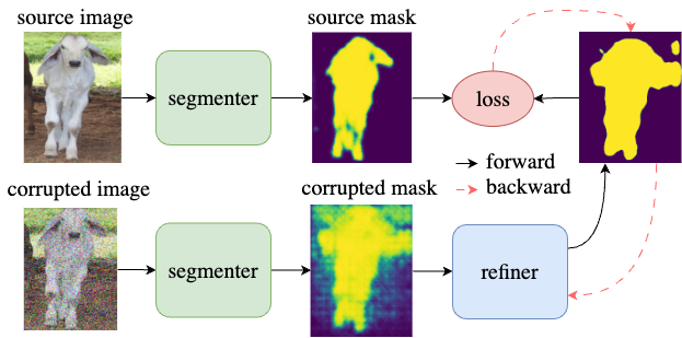
At test-time, adapting to an image $x$, the model parameters are updated to minimize the IoU loss between mask prediction and a refined mask estimated by $f_{\text{R}}$:

$$\theta_{i}^{\star}=\operatorname*{arg\,min}_{\theta_{i}}\mathcal{L}_{\text{IoU}}(f_{\text{R}}(s_{i}),s_{i})$$ (1)

where $\theta_{i}$ are the learnable parameters of $f^{\theta}_{\text{S}}(x)$ and $s_{i}=f^{\theta_{i}}_{\text{S}}(x)$ at iteration $i$.

Refinement module training requires generating masks resembling those that the model would output under domain shift. Instead of swapping input image patches, a heuristic method with many hyper-parameters that could lead to unrealistic artifacts in the masks, this work simulates the mask corruption by using mask predictions on the images from the first few iterations of the Projected Gradient Descent (PGD) [24, 17] adversarial attack, using the inverted mask as target. The more iterations of the attack, the higher the mask corruption. This approach is illustrated in Appendix C. In the first iterations, the most challenging pixels for the network are converted. Similarly, those image areas could be easily impacted by domain shift.

Evaluation metrics The standard semantic segmentation evaluation metric is the mean Intersection over Union (mIoU), where the IoU score of each class is computed from predictions aggregated over the whole dataset

$$\text{mIoU}=\frac{1}{\text{C}}\sum_{c=1}^{\text{C}}\text{IoU}_{c}(m_{c},g_{c})$$ (2)

where $m_{c},g_{c}$ are we predictions and ground truth values for class $c$ for all pixels across all images and $|\text{I}_{c}|$ is the total number of pixels. This metric does not consider the size of objects or the difficulty of individual images. Finally, per-image results can not be compared.

Two additional metrics are introduced to account for the limitations of the standard mIoU. The first metric is designed to consider class imbalance and difficulty of individual images, focusing on per-class performance. It will be referred to as $\text{m}\overline{\text{IoU}}_{c}$ and can be computed as

$$\text{m}\overline{\text{IoU}}_{c}=\frac{1}{\text{C}}\sum_{c=1}^{\text{C}}\frac{1}{|\text{I}_{c}|}\sum_{i\in\text{I}_{c}}\text{IoU}(m_{ic},g_{ic})$$ (3)

where $\text{I}_{c}$ is the set of images in which either the prediction or the ground truth mask contains class $c$.

The second metric is focused on per-image performance and can be computed for a single image. It will be referred to as $\text{m}\overline{\text{IoU}}_{i}$ and can be computed as

$$\text{m}\overline{\text{IoU}}_{i}=\frac{1}{|\text{I}|}\sum_{i\in\text{I}}\frac{1}{|\text{C}_{i}|}\sum_{i\in\text{C}_{i}}\text{IoU}(m_{ic},g_{ic})$$ (4)

where $\text{C}_{i}$ is the set of classes in the predicted masks and the ground truth. Since this work focuses on single-image adaptation and the analyses often require per-image performance, this is the metric reported in most experiments. A similar metric was employed by [41] where the score is determined by averaging the score for the classes in the ground truth only, leading to more optimistic results.

	Ent		PL				Ref				AugCo				Adv		dIoU
params	full	norm	full	full	norm	norm	full	full	norm	norm	full	full	norm	norm	full	norm	full	norm
loss	ent	ent	ce	iou	ce	iou	ce	iou	ce	iou	ce	iou	ce	iou	kl	kl	-	-
NA	35.18	35.18	35.18	35.18	35.18	35.18	35.18	35.18	35.18	35.18	35.18	35.18	35.18	35.18	35.20	35.20	35.18	35.18
$\text{TTA}_{\alpha^{*}}$	35.18	35.58	35.54	37.21	35.60	37.09	35.18	38.69	36.88	36.50	35.27	35.66	35.35	35.39	35.20	35.20	35.18	35.18
$\Delta_{\text{ABS}}$	$-\epsilon$	0.39	0.36	2.03	0.42	1.90	$-\epsilon$	3.51	1.70	1.32	0.09	0.48	0.17	0.21	$-\epsilon$	$-\epsilon$	$-\epsilon$	$-\epsilon$

Table 2: $\text{m}\overline{\text{IoU}}_{i}$ results aggregated across corruptions and levels in the GTA5-C dataset, compared to non-adapted (NA) performance. The TTA hyper-parameters $\alpha^{*}$ were selected for overall best performance of each method. The overall and per-method best results are highlighted. No positive hyper-parameters are denoted by $-\epsilon$ (the performance converges to 0 from below).

Figure 2: GTA5-C error reduction (%) depending on corruption levels. TTA with overall optimal hyper-parameters for COCO-C.

Figure 3: The relationship between per-image scores before and after adaptation on the GTA5-C dataset. The difference between non-adapted (NA) $\text{m}\overline{\text{IoU}}_{i}$ and the $\text{m}\overline{\text{IoU}}_{i}$ after TTA is shown ($\text{m}\overline{\text{IoU}}_{i}\Delta$). A least-squares line fitted to the points in yellow.

Figure 4: The relationship between per-image non-adapted (NA) prediction entropy and TTA $\text{m}\overline{\text{IoU}}_{i}$ improvement on the GTA5-C dataset. The difference between NA $\text{m}\overline{\text{IoU}}_{i}$ and the TTA $\text{m}\overline{\text{IoU}}_{i}$ is shown ($\text{m}\overline{\text{IoU}}_{i}\Delta$). Least-squares line fitted to the points in yellow.

	Ent		PL				Ref				AugCo				Adv		dIoU
params	full	norm	full	full	norm	norm	full	full	norm	norm	full	full	norm	norm	full	norm	full	norm
loss	ent	ent	ce	iou	ce	iou	ce	iou	ce	iou	ce	iou	ce	iou	kl	kl	-	-
NA	55.01	55.01	55.01	55.01	55.01	55.01	55.01	55.01	55.01	55.01	55.01	55.01	55.01	55.01	55.16	55.16	55.01	55.01
$\text{TTA}_{\theta^{*}}$	56.97	56.75	57.17	57.99	57.10	58.30	56.24	57.31	56.56	57.16	55.40	55.59	55.30	56.30	55.16	55.16	55.61	55.74
$\Delta_{\text{ABS}}$	1.96	1.74	2.16	2.98	2.09	3.28	1.23	2.30	1.55	2.15	0.39	0.58	0.29	1.29	$-\epsilon$	$-\epsilon$	0.60	0.73

Table 3: $\text{m}\overline{\text{IoU}}_{i}$ results aggregated across corruptions and levels in the COCO-C dataset, compared to non-adapted (NA) performance. The TTA hyper-parameters $\alpha^{*}$ were selected for overall best performance of each method. The overall and per-method best results are highlighted. No positive hyper-parameters are denoted by $-\epsilon$ (the performance converges to 0 from below).

4 Experiments

The TTA methods are evaluated on two semantic segmentation models pretrained on the GTA5 and COCO datasets. Experiments with each model consist of two parts: 1) Hyper-parameter tuning and analysis on a synthetic validation set and 2) evaluation on real-world datasets with domain shift.

The validation set is based on a set of 40 images from the segmentation model training dataset extended with a diverse set of 9 synthetic corruptions at three corruption levels from [12] such as blur, noise or fog, simulating different domain shifts. Details about the corruptions can be found in Appendix D. These extended datasets based on the GTA5 and COCO datasets are referred to as GTA5-C and COCO-C, respectively. Each validation dataset consists of 1200 images in total. For each TTA method, optimizing either all the network parameters or normalization parameters only is considered, resulting in at least two different setups for each method. Further, when applicable, the cross-entropy and IoU losses are compared. This results in four setups for the Ref, PL and AugCo methods.

Shared implementation details The refinement network architecture is a U-Net [32] with an EfficentNet-B0 [38] backbone pre-trained on ImageNet from the Timm library [46]. It is trained with the AdamW [23] optimizer with a learning rate of $1e^{-3}$ and the Cross-Entropy (CE). The SGD optimizer is used for TTA and the hyper-parameters considered during validation are the learning rate and number of TTA iterations. The maximum possible number of iterations is 10 to limit the computational requirements. Early experiments with AdamW for TTA showed high divergence rate.

Figure 5: COCO-C error reduction (%) depending on corruption levels. TTA with overall optimal hyper-parameters for COCO-C.

4.1 GTA5 $\rightarrow$ Cityscapes, ACDC

The GTA5-pretrained model is the best-performing model of [41] (DeepLabV2). The results of different methods with parameters selected for the overall best performance across all corruptions and levels can be found in Table 2. It can be observed that largely improved results are achieved either by PL with IoU loss, optimizing normalization parameters only, or by Ref with IoU loss, optimizing all the parameters. The best-performing method is Ref, improving by 3.51 % over the non-adapted baseline (NA), reducing the total segmentation error by 5.41 %. Other methods only marginally improve over NA or show no improvement at all. Optimizing CE generally yields worse results than IoU. While updating normalization parameters may only stabilize Ent, optimizing all the parameters for optimal performance of Ref is important. For other methods, the difference is small, yet optimizing normalization parameters only is faster and thus recommended.

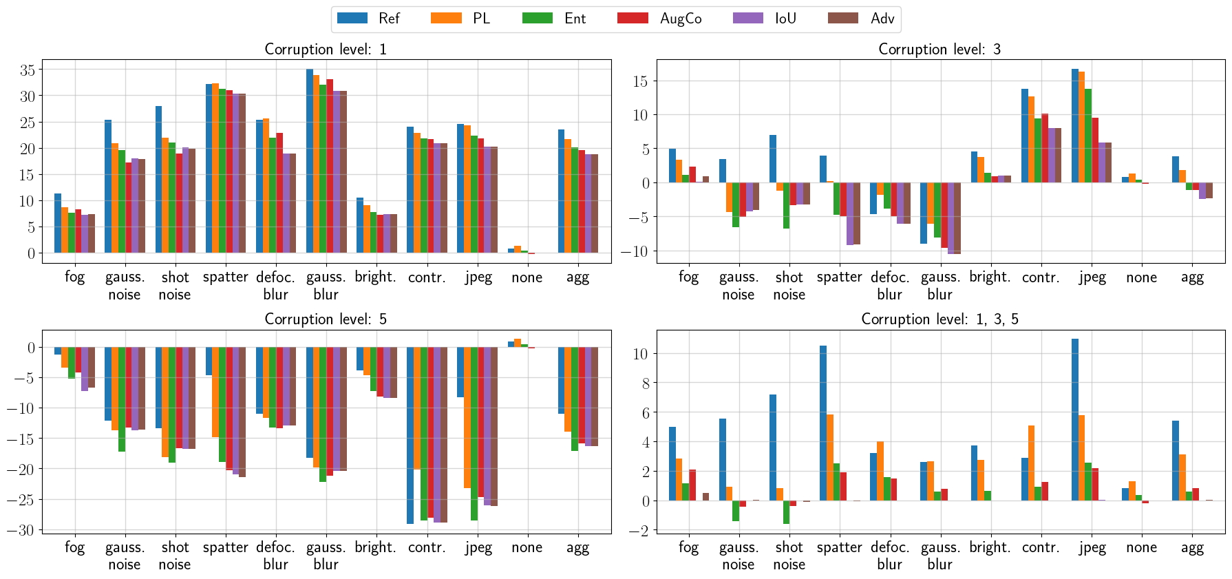
In Figure 2, the total error reduction results with a single set of optimal hyper-parameters for each method are reported for each corruption level and kind. Results show that it is not possible to find a single set of hyper-parameters that would perform well across all the corruption levels with current methods. While all methods improve performance on level 1 corruptions, from level 3, negative results can be observed for some of the corruptions, and all methods yield negative results on level 5. Ref outperforms the other methods on the majority of corruption kinds and corruption levels. Aggregated results across all corruptions show that the negative results for level 5 and mixed results for level 3 are mostly outweighed by the gains on level 1, resulting in overall positive results. This analysis suggests that unless it is known in advance what kind of corruption or corruption levels will be present after deployment, strategies on method and hyper-parameter selection for each image should be considered.

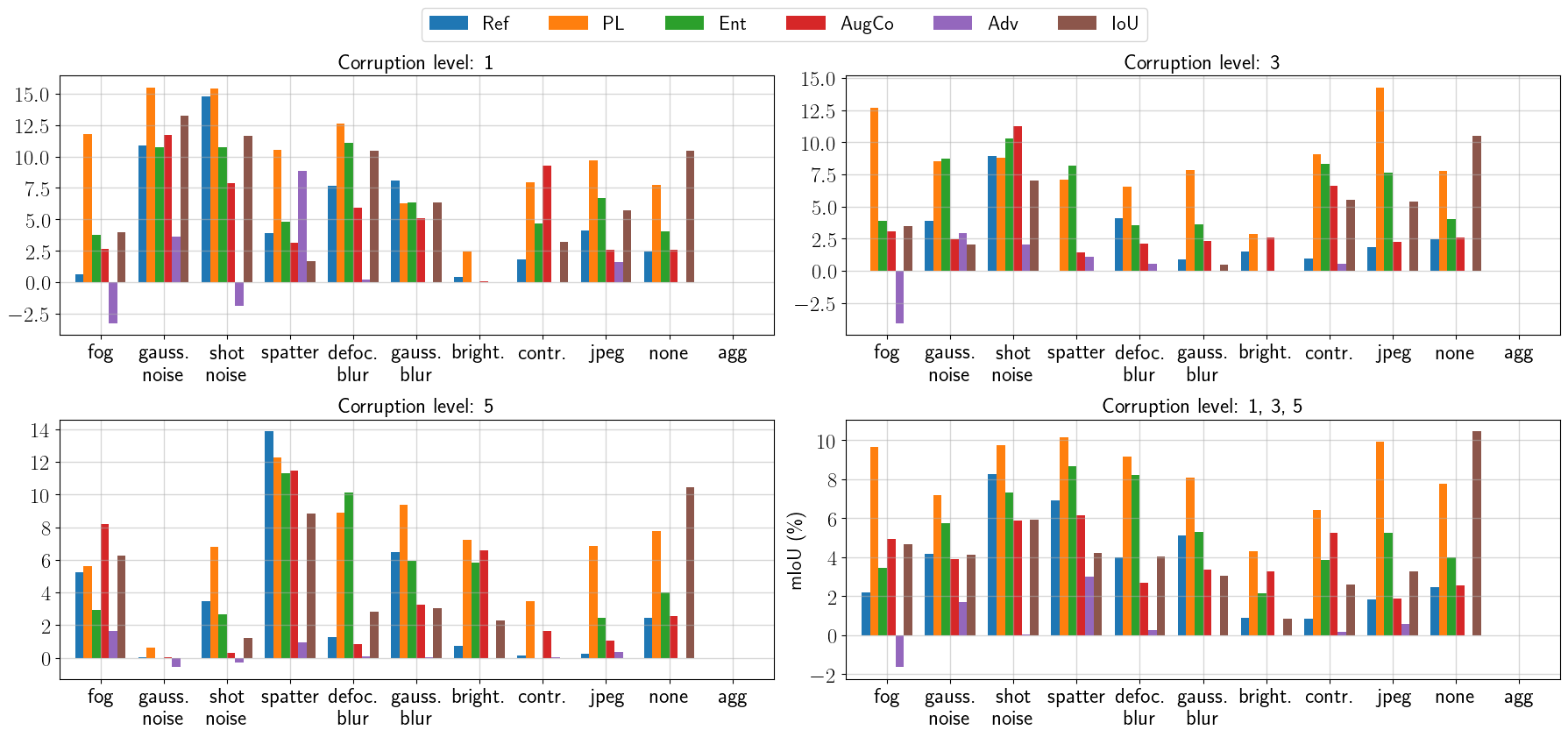
In Appendix E, it is shown that if one could select optimal hyper-parameters for each method, corruption kind and level, results would improve substantially. Moreover, Ref significantly outperforms the other methods on most corruptions, the blur corruption kinds being a notable exception. Significant improvements can be observed compared to other methods, especially on different kinds of noise and jpeg corruption at level 5.

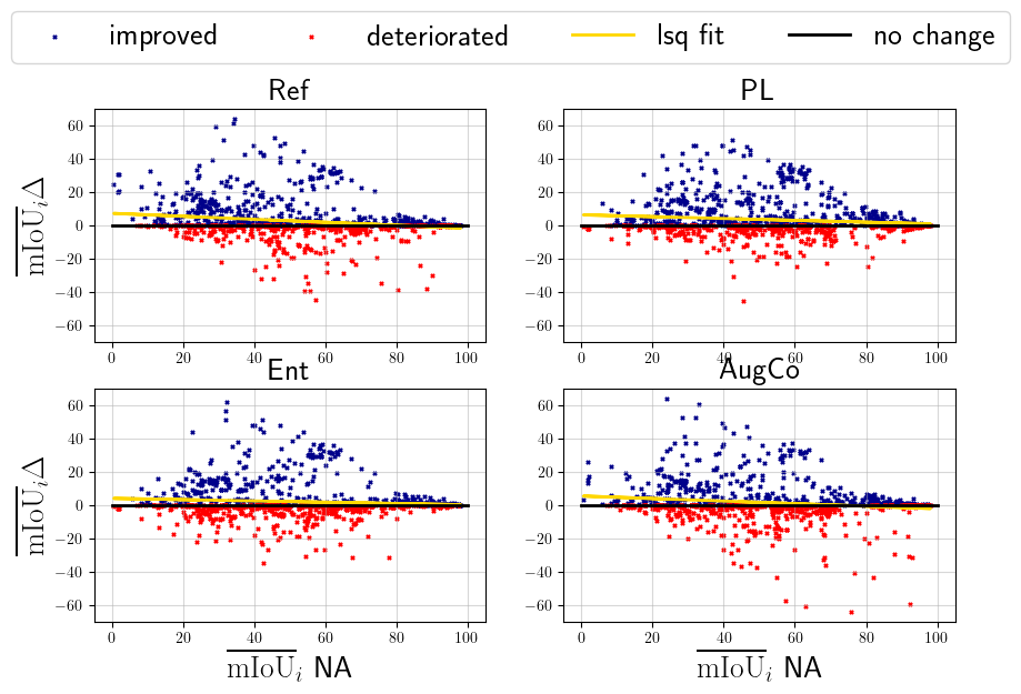
Only the methods with positive TTA results are used for further analysis, namely Ref, PL, AugCo and Ent. Finally, the relationship between the non-adapted (NA) performance and the performance improvement on individual images for different methods is visualized in Figure 3. The analysis shows Ref outperforms other methods, especially on images that had low initial $\text{m}\overline{\text{IoU}}_{i}$, while the performance of PL is consistent across all initial scores yet not as powerful for initial low scores. While Ent makes performance worse for low initial scores and improves more as the initial score increases, AugCo shows consistent improvements across all initial scores similarly to PL, yet to a smaller extent.

Figure 6: TTA $\text{m}\overline{\text{IoU}}_{i}$ error reduction (%) of GTA5 model on the driving test datasets with hyper-parameters selected on GTA5-C.

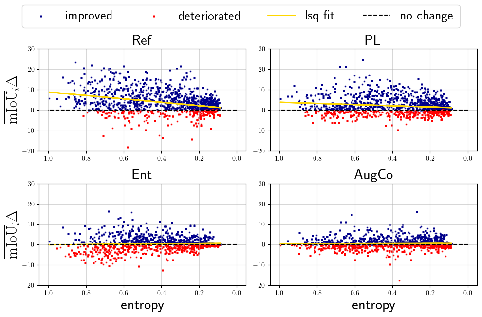
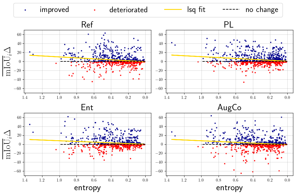
If the $\text{m}\overline{\text{IoU}}_{i}$ for each image were known, it could be used to either select a method performing best on those values or to select hyper-parameters. In Figure 4, an analogous analysis is performed, replacing the $\text{m}\overline{\text{IoU}}_{i}$ with segmentation prediction entropy. Similar results as with the $\text{m}\overline{\text{IoU}}_{i}$ can be observed, showing that the segmentation prediction entropy is a good proxy for initial segmentation $\text{m}\overline{\text{IoU}}_{i}$.

After the best hyper-parameters for each method are selected on the validation set, the methods are evaluated on 5 test datasets: ACDC-Rain, ACDC-Fog, ACDC-Night and ACDC-Snow, and Cityscapes. The Cityscapes represents a domain shift from synthetic to real images. The first four datasets are created by splitting the ACDC dataset by different conditions and, apart from the synthetic to real, further represent adverse weather conditions domain shift. Each test set consists of 500 images.

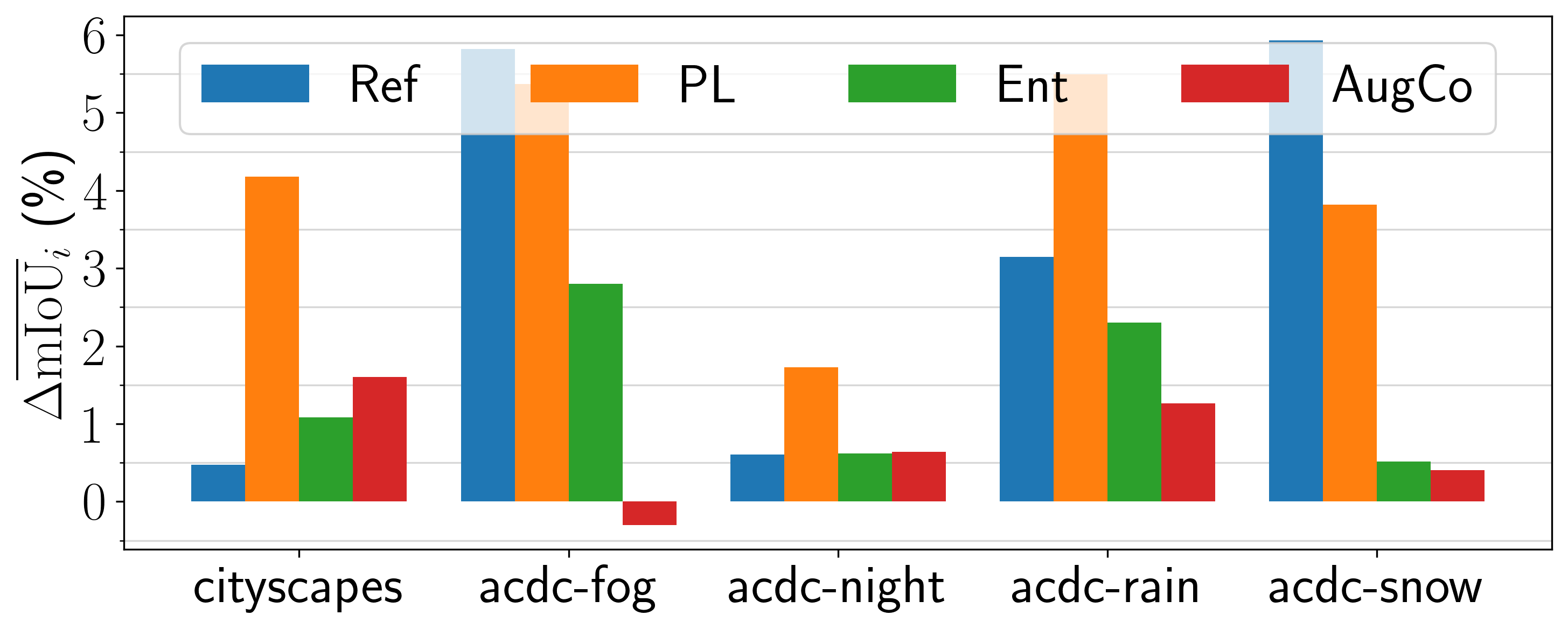
The test results are reported in Figure 6. Similar to validation, the Ref and PL methods perform best across all datasets. While not outperforming Ref on all the datasets, the performance of PL is consistently better than the other methods while Ref is outperformed or matched by the other methods on Cityscapes and ACDC-night.

4.2 COCO $\rightarrow$ VOC

The segmentation model is an official Torchvision DeepLabV3 with Resnet50 backbone trained on the COCO dataset with a subset of 20 VOC classes. The results of different methods with parameters selected for the overall best performance across all corruptions and levels can be found in Table 3. Major improvements are obtained by the PL and Ref methods. PL outperforms Ref, in contrast to GTA5-C experiments. The best improvement is by 3.28 %, reducing the total segmentation error by 7.3 %. Again, best results for each method are always achieved by IoU, outperforming CE in all cases. In contrast to GTA5-C, Ent achieves better results when optimizing all the network parameters. The same holds for PL. For Ref, optimizing all the parameters is important. For most methods, the difference is small; overall, improvements over the non-adapted baseline are marginal.

Figure 7: The relationship between per-image scores before and after adaptation on the COCO-C dataset. The difference between non-adapted (NA) $\text{m}\overline{\text{IoU}}_{i}$ and the $\text{m}\overline{\text{IoU}}_{i}$ after TTA is shown ($\text{m}\overline{\text{IoU}}_{i}\Delta$). A least-squares line fitted to the points in yellow.

Figure 8: The relationship between per-image non-adapted (NA) prediction entropy and TTA $\text{m}\overline{\text{IoU}}_{i}$ improvement on the COCO-C dataset. The difference between NA $\text{m}\overline{\text{IoU}}_{i}$ and the TTA $\text{m}\overline{\text{IoU}}_{i}$ is shown ($\text{m}\overline{\text{IoU}}_{i}\Delta$). Least-squares line fitted to the points in yellow.

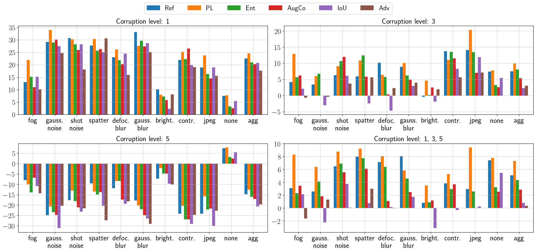
The total error reduction results with a single set of optimal hyper-parameters for each method are reported for each corruption level and kind in Figure 5. The results slightly differ from those for the GTA5-C, as in this case, PL outperforms Ref. Both methods are again consistently better than the other methods, but positive results are reported for most corruptions on both level 1 and level 3.

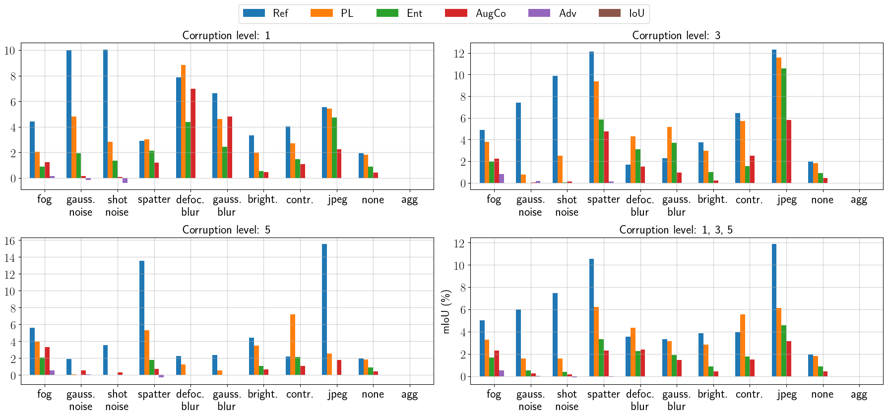
In Appendix E, the results with optimal hyper-parameters for each method, corruption kind, and level are shown. This time, the results between different methods are much smaller. The PL consistently outperforms all other methods at all the corruption levels. Interestingly, the dIoU methods shows much stronger performance than in the GTA5-C experiments.

Again, only Ref, PL, AugCo and Ent are used for further analysis. The relationship between the non-adapted (NA) performance and the performance improvement on individual images for different methods is visualized in Figure 7. The distribution of initial non-adapted $\text{m}\overline{\text{IoU}}_{i}$ is different. The initial model is stronger than the GTA5 model. All methods show similar behavior - more improvement is achieved on images with a lower initial score, Ref and PL significantly outperform the other methods and again, Ref show better performance on images with low initial scores compared to other methods.

The relationship of segmentation prediction entropy and $\text{m}\overline{\text{IoU}}_{i}$ improvement by adaptation is shown in Figure 8, supporting the notion that the entropy of prediction before adaptation is a good proxy for $\text{m}\overline{\text{IoU}}_{i}$.

Figure 9: TTA $\text{m}\overline{\text{IoU}}_{i}$ error reduction (%) of COCO model on the VOC test dataset with hyper-parameters selected on COCO-C.

The results on the VOC test set are shown in Figure 9. PL slightly outperforms the other methods, but all the methods improved over the non-adapted baseline.

Additional results can be found in Appendix E.

5 Conclusions and Discussion

The first finding is that all the methods minimizing the CE loss can be improved by optimizing the IoU loss. Optimizing all the network parameters, compared to optimizing the normalization parameters only, is shown to bring large performance gains for the Ref method, making it another important hyper-parameter to consider. With these improvements, we identify PL and Ref as the overall best-performing methods. The performance is improved by 3.51 % and 3.28 % on GTA5-C and COCO-C validation sets, while without IoU loss, the improvements would have been by 1.7 % 2.16 % only. This could be explained by the fact that IoU loss is better suited for highly-imbalanced data. The imbalance is even stronger for the single-image setup.

The experiments further reveal that even though the methods achieve impressive performance gains when optimizing hyper-parameters for each corruption and corruption level separately, there is a huge performance drop when evaluating with a single set of hyper-parameters. This results in negative performance on many corruptions. It is also shown that Ref performs better compared to PL when the segmentation quality before adaptation is low, while it may deteriorate performance on already high-quality masks. Entropy is shown to be a good estimate of the quality. This reveals the great potential of learnt refinement modules for severe domain shifts but also highlights the need for improvements in the training of the module to ensure performance is not degraded for high-quality masks.

The Ent baseline is often reported as too unstable for single-image adaptation, producing negative results. In contrast, [41], and our experiments show positive results. The difference is that our work and [41] do not update the batch normalization statistics like the original work proposes, only the learnable parameters.

Finally, the test results further highlight that it is not possible to find a single set of hyper-parameters for the tested TTA, since the results do not always reflect those on the validation set. If the domain shift kind is known, the validation set can be tuned to these conditions, but that undermines the idea of adapting to an arbitrary unknown domain shift - if the conditions are known in advance, there are many techniques to exploit that information.

Limitations First, a single isolated image adaptation by optimizing model parameters has a high computational cost, as a backward operation is required for each iteration. If such methods are to be broadly adopted, this issue should be addressed. Further, many of the methods evaluated in this work were not designed with single-image adaptation in mind, and modifications were necessary. Poor performance in our benchmarks does not invalidate the performance of the methods in the setup these were proposed for. Finally, some of the methods have not made the code public. The code with the methods reimplementation will be released.

Appendix A Related setups

Domain adaptation methods share a lot in common with semi-supervised learning [31, 33] and may exploit strategies such as generative models [39, 47]. In practice, this is often infeasible since source data may not be available for example for privacy reasons, or we may only have a small number of target domain images available. In continually evolving environments, the distribution may have already changed by the time adaptation on a whole target dataset is completed. Various modifications of the traditional domain adaptation scenario tackling the aforementioned limitations have recently emerged, for example by considering no access to source data or a continual domain shift [22, 41, 44, 3]. In particular, test-time adaptation methods assume no source data is available and aim to exploit the information from as little as a single target domain image.

TTA can also be described as source-free unsupervised domain adaptation. A model trained on a source domain has to adapt to a target domain without access to the source data and without any labels. Let us first describe related terms and also the difference between similar but different setups that may be easily confused:

Continuous domain adaptation assumes the target data change continually, as opposed to a static target distribution. Furthermore, it is important to avoid catastrophic forgetting (previous knowledge). In this work, we make no assumption about the relationship between the distribution of subsequent samples, each sample could come from a different distribution. For this reason, our models are initialized to the pretrained weights before adapting to a new image and catastrophic forgetting is not a concern. While single-image adaptation methods can be extended to continual learning, it is not clear that methods performing better in the single-image setup will also perform better in batch or stream of data mode.

Domain generalization aims for a strong model that would generalize to unseen domains without any adaptation. Common approaches are domain-invariant representation learning, data augmentation or data generation. In contrast, this work focuses on adapting a pre-trained model to become a specialist in the current domain. It was shown in [41] that a stronger, more general model can lead to better adaptation results, making these directions complementary. However, without adaptation, training a very general model on a large set of distributions may harm the model’s performance on the individual distributions when compared to specialized models with carefully optimized data augmentation [1, 36].

Online domain adaptation expects a stream of data as input, possibly a single one, as opposed to a whole dataset. Test-time adaptation methods can be sued for online adaptation but generally, online adaptation techniques do not assume the source data are not available.

Zero-shot segmentation requires the model to directly perform predictions for previously unseen classes without any adaptation to these classes.

Appendix B Baseline methods

In this section, the self-supervised loss functions optimized in the baseline methods are described, as well as the adaptations from the original implementation to the single-image setup when necessary.

B.1 Entropy Minimization (Ent)

The Ent method minimizes the entropy of the segmentation predictions. In the context of learning with limited supervision, it was proposed in [11] for semi-supervised learning. In TTA, there is no labelled set that could be leveraged as regularization like in semi-supervised learning but the methods were shown to work for TTA as well [43]. It was also shown that larger batch size and updating the parameters of the normalization-layers only improve stability of the method. But on segmentation, a dense-prediction task, adapting to a single image can lead to positive results, especially when not updating the batch normalization statistics but only the learnable parameters like in [41].

The method is simple, computationally efficient and widely adopted as a baseline. More formally, the method minimizes the entropy of the segmentation model predictions $s=f^{\theta}_{\text{S}}(x)$ for an image $x$:

$$\mathcal{L}_{\text{Ent}}=\sum_{i=1}^{\text{N}}\sum_{i=1}^{\text{C}}\text{s}_{ic}\cdot\log(\text{s}_{ic})$$ (5)

where C is the total number of classes, $\text{s}_{ic}$ corresponds to the $i$-th pixel of the segmentation prediction s for class $c$ and N is the total number of pixels in the image.

In this work, the batch normalization [14] statistics are not updated since it relies on the presence of batch normalization layers while many recent architectures use other normalization layers such as layer normalization [2].

B.2 Pseudolabelling (PL)

Pseudolabelling also comes from semi-supervised learning [18] and is based on the idea of using the segmentation prediction of an image (prediction for each class binarized through argmax) as ground truth to optimize the model. In effect, it is the same as pseudo-labelling since both methods reduce class overlap. However, pseudolabelling has the advantage of allowing for different loss function. While the CE loss is typically optimized, our experiments show that in the single image setup, IoU leads to superior results.

B.3 Adversarial Transformation Invariance (Adv)

This method is an extension of TIPI (Test-Time Adaptation with Transformation Invariance) by [27] to image segmentation. The main idea is to make the network invariant to adversarial transformation of the input image as a representative of domain shifts.

The optimization loss is computed as the reverse KL divergence loss between the model prediction $s^{\prime}=f^{\theta}_{\text{S}}(x^{\prime})$ where $x^{\prime}$ is an adversarially transformed image and the prediction on the original input $s=f^{\theta}_{\text{S}}(x)$.

$$\mathcal{L}_{\text{Adv}}=\mathcal{L}_{\text{KL}}(\text{s}_{i},\text{s}^{\prime}_{i})$$ (6)

where $\text{s}^{\prime}_{i}$ is the adversarially transformed prediction and KL is the Kullback-Leibler divergence loss defined as

$$\mathcal{L}_{\text{KL}}(\text{p},\text{q})=\frac{1}{N}\sum_{i=1}^{N}\text{q}_{i}\cdot\log(\frac{\text{q}_{i}}{\text{p}_{i}})$$ (7)

In forward KL, p corresponds to the model prediction while q to the ground truth. Please note that, as suggested in [27], the reverse KL is used in the proposed method where the input arguments to the function are switched, compared to forward KL. Another important implementation detail is that the gradients should not flow through $\text{s}^{\prime}_{i}$ - the tensor needs to be detached before the loss computation.

The same adversarial attacks in terms of the ground truth as for the IoU estimation and mask refinement methods are used to generate $x^{\prime}$ but the computational complexity is reduced by using the Fast Gradient Sign Attack (FGSM) proposed in [10].

Importantly, two sets of batch normalization statistics are kept in [27], which is not done in our work due to the aim for general methods that do nto assuem the presence of specific network layers. This may be the reason why the methods perform poorly in our experiments. Another thing we ntoed is the high variance of the KL loss.

B.4 Augmentation Consistency (AugCo)

Figure 10: Visualization of the predicted views, confidence, consistency and reliablity (confident $|$ reliable) masks used by the AugCo TTA method. Confident/consistent/reliable predictions are shown in yellow.

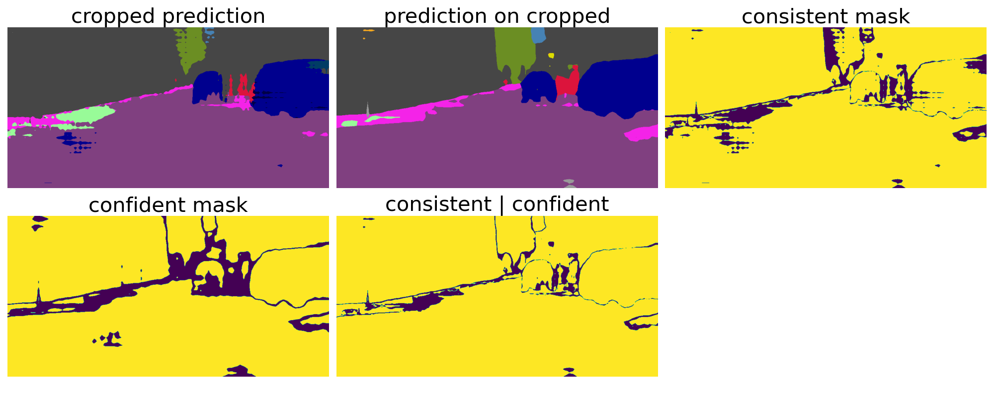
The method of [29] is adapted to the single image setup. The idea is to create two segmentation views based on the input image, both based on a random bounding box with parameters $\alpha$. The bounding box should take 25-50 % of the original image area and preserve its aspect ratio. View 1 is created by cropping and resizing the segmentation of the original image, $V_{1}=\text{resize}(\text{crop}_{\alpha}(s),\text{H},\text{W})$ where $s=f^{\theta}_{\text{S}}(x)$ is the segmentation prediction for an image $x$ of spatial dimensions $\text{H},\text{W}$. View 2 is created as the segmentation prediction on a cropped, resized and randomly augmented image, $V_{2}=f^{\theta}_{\text{S}}(x^{\prime})$ where $x^{\prime}=\text{resize}(\text{crop}_{\alpha}(\text{jitter}(x)),\text{H},\text{W})$.

Finally, two masks are created to identify reliable predictions: Consistency mask based on consistency between the predictions of the two views, and confidence mask based on the confidence in the prediction in $V_{2}$, binarized with a confidence threshold $\theta$. These are then combined with the $\mathrm{OR}$ operation. We set $\theta=0.8$.

The network parameters are then updated via pseudo-labelling based on predictions of $V_{2}$ and using reliable pixels only.

In [29], an auxiliary information entropy loss preventing trivial solutions is also optimized. This loss requires running class-frequency statistics and is not applicable to the single-image setup. Further, an adaptive threshold based on per-class confidence distirbution in a batch of images is computed iinstead of a fixed threshold, which is also not applicable in our setup.

An example of the two views and the consistency and confidence masks, as well as the resulting reliability masks, are shown in Figure 10. For more details please see the original work.

Appendix C Adversarial refinement training

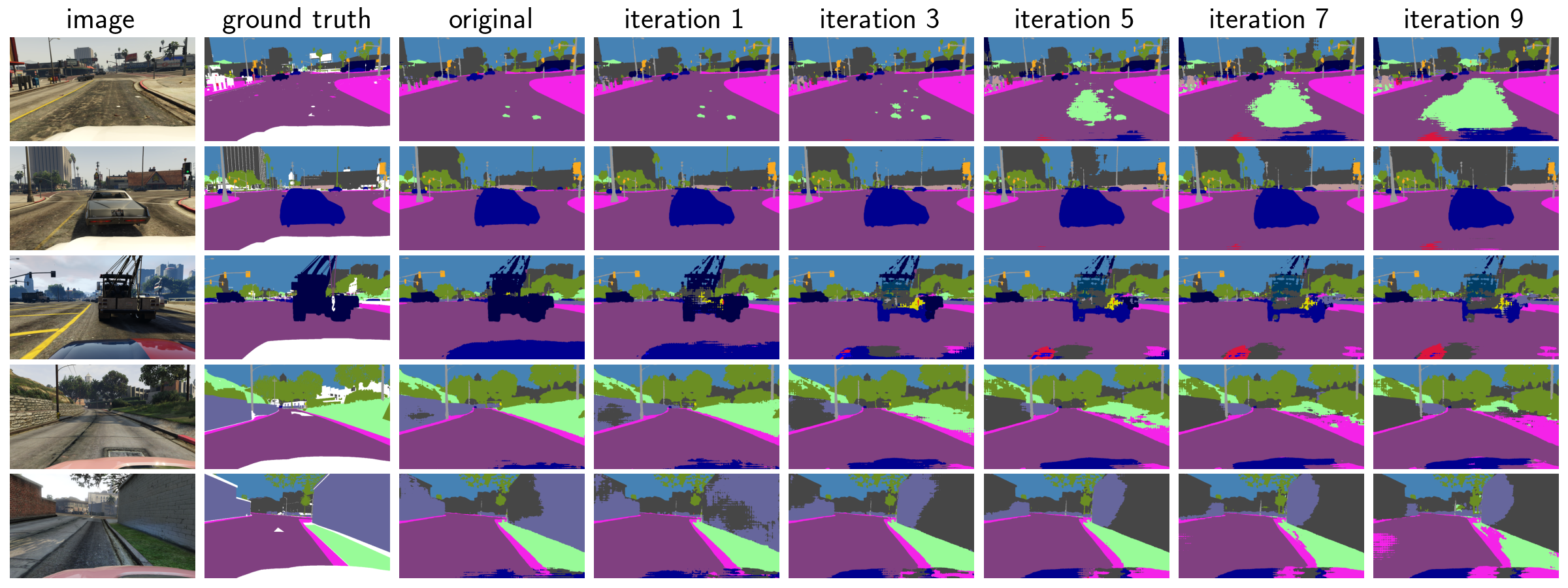
A visulaisation of mask evolution as the adversarial attack progresses is shown in Figure 11. It can be observed that the first iterations typically result in very small changes in easily confused areas, turning into more and more distorted masks.

Figure 11: Evolution of masks over iterations of a projected gradient descent adversarial attack on the input image, the target being mask inversion for all of the classes. These masks serve as training data for the refinement module.

Instead of the iterative Projected Gradient Descent (PGD). However, since the projection only consists in restricting the output to a valid range for an image, typically implemented by simply clipping the output, it is also often referred to as iterative FGSM.

Appendix D Synthetic corruptions

The corruptions used in our experiments are a subset of the corruptions from [12]. An overview of the corruptions, as well as implementation details, can be found in Table 4

corruption	description
brightness	is an additive intensity transformation, $x_{c}=\text{clip}(x+b)$ where $b$ controls the level.
contrast	is a multiplicative intensity transformation, $x_{c}=b(x-\overline{x})+x$ where $b$ controls the level and $\overline{x}$ is a per-channel mean of the image intensities.
frost	first crops a portion of one of the frost image templates at a random location of the same size as the input image, $x_{\text{f}}$. Then we compute $x_{c}=b_{1}x+b_{2}x_{\text{f}}$ where the weights $b_{1},b_{2}$ control the level.
fog	first generates a heightmap $x_{\text{h}}$ using the diamond-square algorithm [7], where the wibble is controlled by a parameter $b_{1}$. It is then combined with the input image as $x_{c}=\frac{(x+b_{1}\cdot x_{\text{h}})\cdot\max(x)}{\max(x)+b_{1}}$.
gaussian noise	is generated as $x_{c}=x+n$ where $n\sim\mathcal{N}(0,b)$ and $b$ controls the level.
shot noise	is generated as $x_{c}\sim\frac{\text{Pois}(x\cdot b,\lambda=1)}{b}$ where Pois denotes the Poisson distribution and $b$ controls the level.
spatter	simulates mud or water spoiling. The main idea of the algorithm is a combination of thresholding and blurring random noise.
defocus blur	first generates a disk kernel K with radius $b_{1}$ and alias blur $b_{2}$. The kernel is then used to filter each of the channels $x_{c}=\text{K}(x)$.
gaussian blur	corrupts the image by gaussian blurring $x_{c}=\mathcal{N}(x,b)$ where $b$ controls the level.
jpeg	is computed as $x_{c}=\text{jpeg}(x,b)$ where jpeg performs the JPEG compression with quality $b$.

Table 4: Corruptions and their implementation details, a subset from [12]. The input of the transformation is an image $x$ normalized to the $(0,1)$ range, the output is a corrupted image $x_{c}$. The clip function limits the values to the $[0,1]$ range. This function is always applied to the output image after the transformation to obtain the final output $x_{f}=\text{clip}(x_{c})$. For more details on the transformations and the values defining the level, please refer to the codebase.

Appendix E Additional experimental results

		method
dataset	metric	NA	Ref	PL	Ent	AugCo
Cityscapes	$\text{m}\overline{\text{IoU}}_{i}$	34.40	34.71	37.14	35.11	35.45
	$\text{m}\overline{\text{IoU}}_{c}$	28.71	28.64	30.70	29.09	29.48
ACDC-fog	$\text{m}\overline{\text{IoU}}_{i}$	32.03	35.98	35.67	33.93	31.82
	$\text{m}\overline{\text{IoU}}_{c}$	24.87	27.29	27.52	26.00	24.69
ACDC-night	$\text{m}\overline{\text{IoU}}_{i}$	13.60	14.12	15.09	14.13	14.15
	$\text{m}\overline{\text{IoU}}_{c}$	10.77	10.96	11.53	10.68	11.01
ACDC-rain	$\text{m}\overline{\text{IoU}}_{i}$	33.52	35.61	37.17	35.05	34.36
	$\text{m}\overline{\text{IoU}}_{c}$	26.15	27.40	28.47	26.89	26.66
ACDC-snow	$\text{m}\overline{\text{IoU}}_{i}$	31.54	35.60	34.15	31.89	31.81
	$\text{m}\overline{\text{IoU}}_{c}$	25.28	28.09	27.17	25.39	25.45

Table 5: ACDC and Cityscapes test datasets results. Hyper-parameters were selected for overall best performance on GTA5-C. Best results for each dataset and metric are highlighted.

	method
metric	NA	Ref	PL	Ent	AugCo
$\text{m}\overline{\text{IoU}}_{i}$	77.03	78.21	79.83	78.66	77.75
$\text{m}\overline{\text{IoU}}_{c}$	63.31	64.54	67.13	65.02	63.27

Table 6: VOC test dataset results. Hyper-parameters were selected for overall best performance on COCO-C. Best results for each dataset and metric are highlighted

Figure 12: GTA5-C: $\overline{\text{IoU}}_{c}$ per-class comparison of different TTA methods.

Validation results

		$\text{m}\overline{\text{IoU}}_{i}$
dataset	trained on	non-adapted	TTA
COCO-C	predictions	55.01	57.31
	gts	55.01	55.88
GTA5-C	predictions	35.18	38.63
	gts	35.18	38.69

Table 7: Comparison of training the refinement module with ground truth masks and with segmentation model predictions. The $\text{m}\overline{\text{IoU}}_{i}$ aggregated across all corruption types and levels is reported with overall optimal hyper-parameters for each dataset.

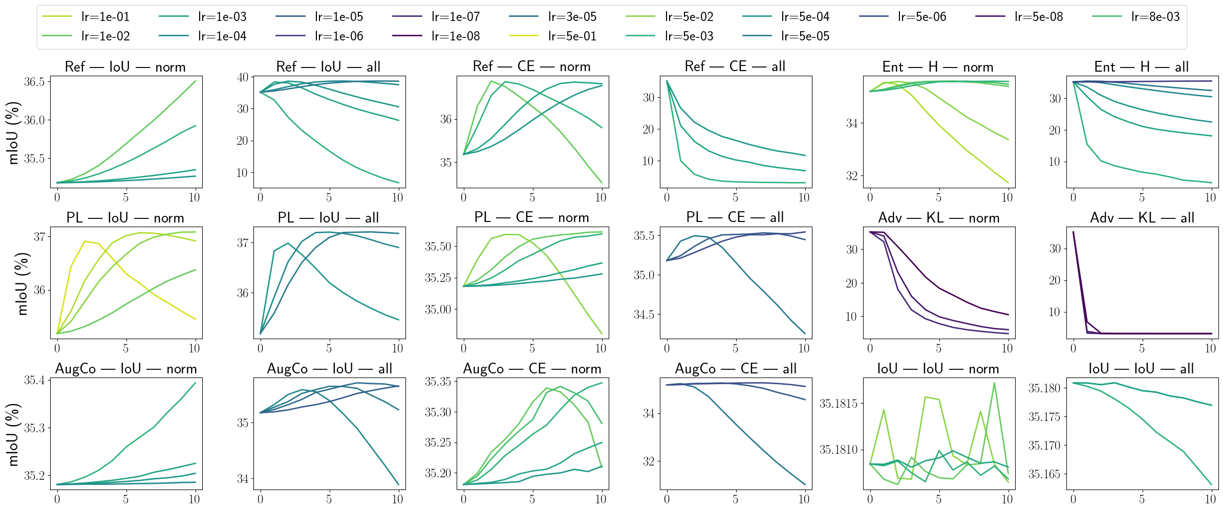
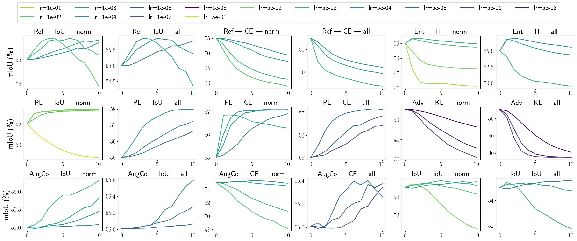
The evolution of $\text{m}\overline{\text{IoU}}_{i}$ over TTA iterations depending on the hyper-parameters on the GTA5-C validation set can be found in Figure 13. The same results for the COCO-C validation dataset can be found in Figure 14.

Figure 13: GTA5: $\text{m}_{i}\overline{\text{IoU}}$ evolution over 10 TTA iterations as a function of the learning rate. The results are reported as ‘method - loss - optimized parameters’. The y-axes scale differs for each subplot to better visualize learning-rate differences for each method.

Figure 14: COCO-C: $\text{m}_{i}\overline{\text{IoU}}$ evolution over 10 TTA iterations as a function of the learning rate. The results are reported as ‘method - loss - optimized parameters’. The y-axes scale differs for each subplot to better visualize learning-rate differences for each method.

Figures 16 (GTA5-C) and 15 (COCO-C) show the results when optimal hyper-parameters are determined for each corruption and level separately. These results show that the performance improves substantially compared to the scenario with overall optimal hyper-parameters for all corruptions and levels. Further, while on the GTA5-C dataset, Ref sinigificantly outperforms the other methods, PL is better in the VOC-C benchmark.

Figure 15: Comparison of total error reduction across methods per corruption levels on COCO-C dataset

Figure 16: Comparison of total error reduction across methods per corruption levels on GTA5-C dataset

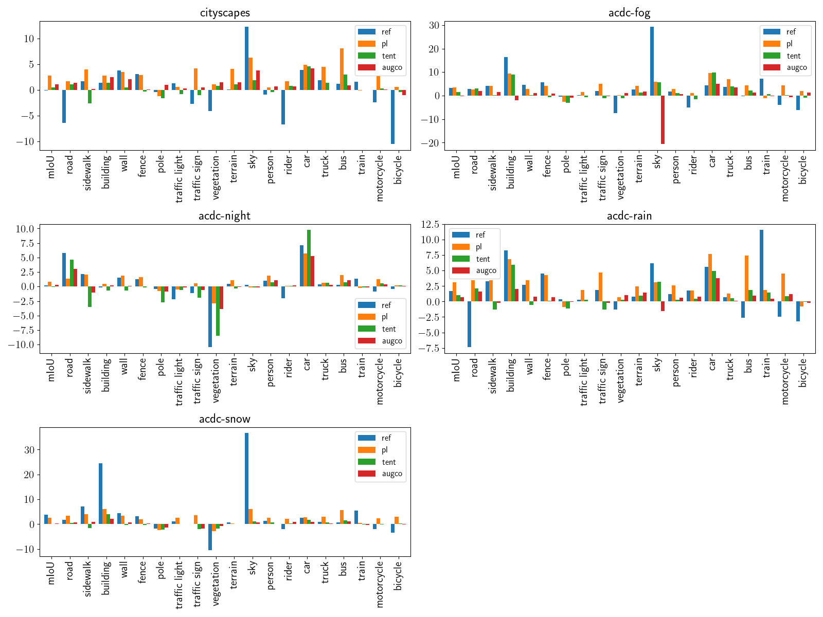
Test results The $\text{m}\overline{\text{IoU}}_{c}$ comparison for all classes on the ACDC and Cityscapes test datasets can be found in Figure 12.

The numerical results on the Cityscapes and ACDC test dataset can be found in Table 5, showing different methods may perform better depending on the evaluation metric. The same results for the VOC test dataset are shown in Table 6.

Additional experiments The refinement module is trained to predict a clean mask based on a corrupted mask simulating masks processed by the model under domain shift. The clean mask can be the segmentation prediction on clean, non-corrupted images or, when available, ground truth masks can be used instead. Comparison of these two choices is shown in Table 7. The results are somewhat inconclusive - for the COCO model it can be seen that the model trained on predictions is substantially better than the one trained on ground truth. The GTA5 model performs similarly in both cases. One could argue that learning with GT can compensate for some of the mistakes even source distribution images, since prediction form output space back to output space is different then prediction from image to output space. On the other hand, when predictions differ significantly from ground truth even on source distirbution images, it can result in noiser data and more difficult training. The choice should be validated experimentally for each model and dataset.

Figure 17: Segmentation evolution during TTA with Ref on VOC test set. First row shows the evolution of masks, second row shows the input image and segmentation improvement w.r.t. to the non-adapted mask. Improved and deteriorated pixels are highlighted.

Figure 18: Segmentation evolution during TTA with Ref on ACDC-fog test set. First row shows the evolution of masks, second row shows the input image and segmentation improvement w.r.t. to the non-adapted mask. Improved and deteriorated pixels are highlighted.

Figure 19: Segmentation evolution during TTA with Ref on ACDC-night test set. First row shows the evolution of masks, second row shows the input image and segmentation improvement w.r.t. to the non-adapted mask. Improved and deteriorated pixels are highlighted.

Figure 20: Segmentation evolution during TTA with Ref on ACDC-snow test set. First row shows the evolution of masks, second row shows the input image and segmentation improvement w.r.t. to the non-adapted mask. Improved and deteriorated pixels are highlighted.

Figure 21: Segmentation evolution during TTA with Ref on ACDC-rain test set. First row shows the evolution of masks, second row shows the input image and segmentation improvement w.r.t. to the non-adapted mask. Improved and deteriorated pixels are highlighted.

Figure 22: Segmentation evolution during TTA with Ref on cityscapes test set. First row shows the evolution of masks, second row shows the input image and segmentation improvement w.r.t. to the non-adapted mask. Improved and deteriorated pixels are highlighted.

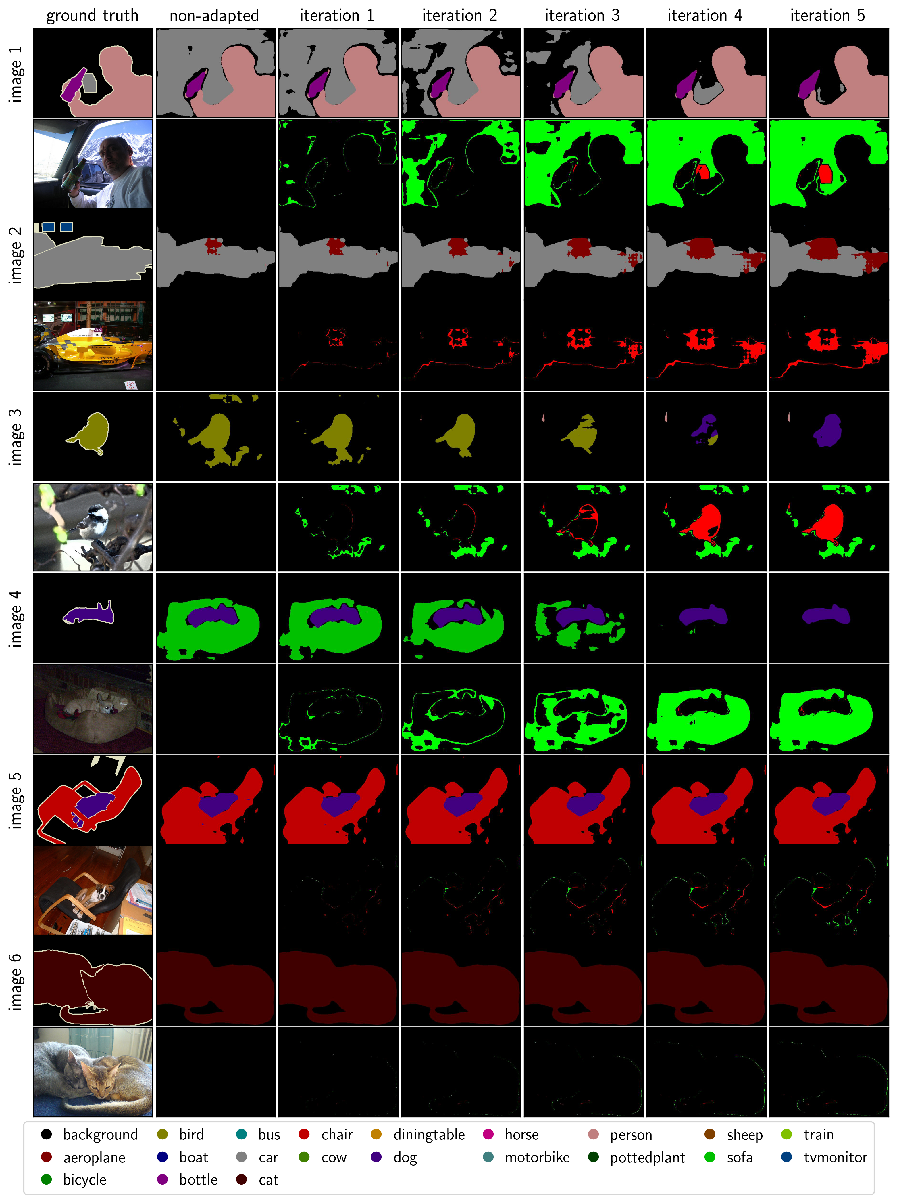
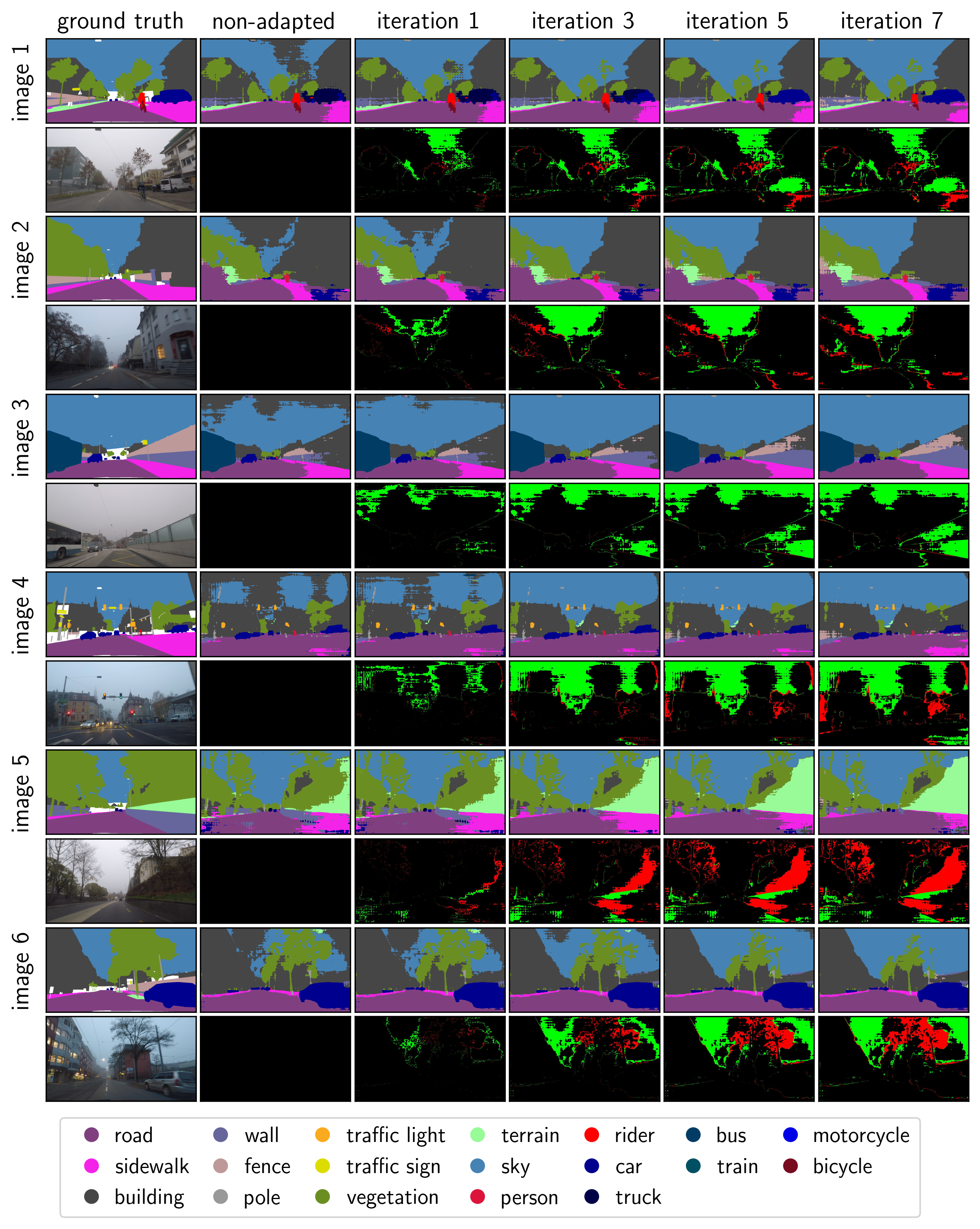
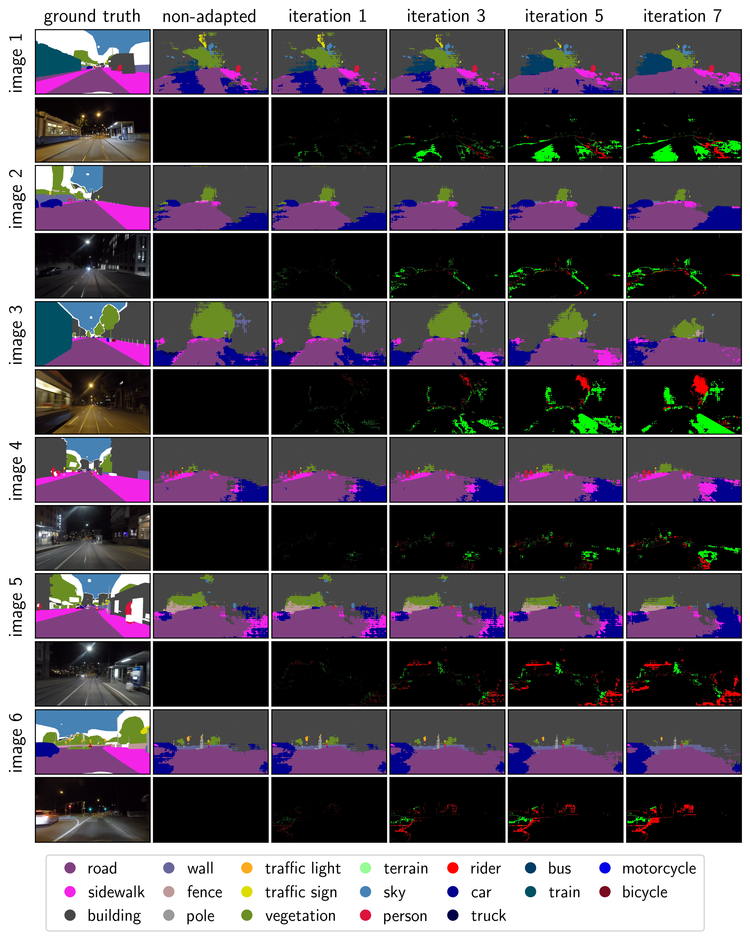
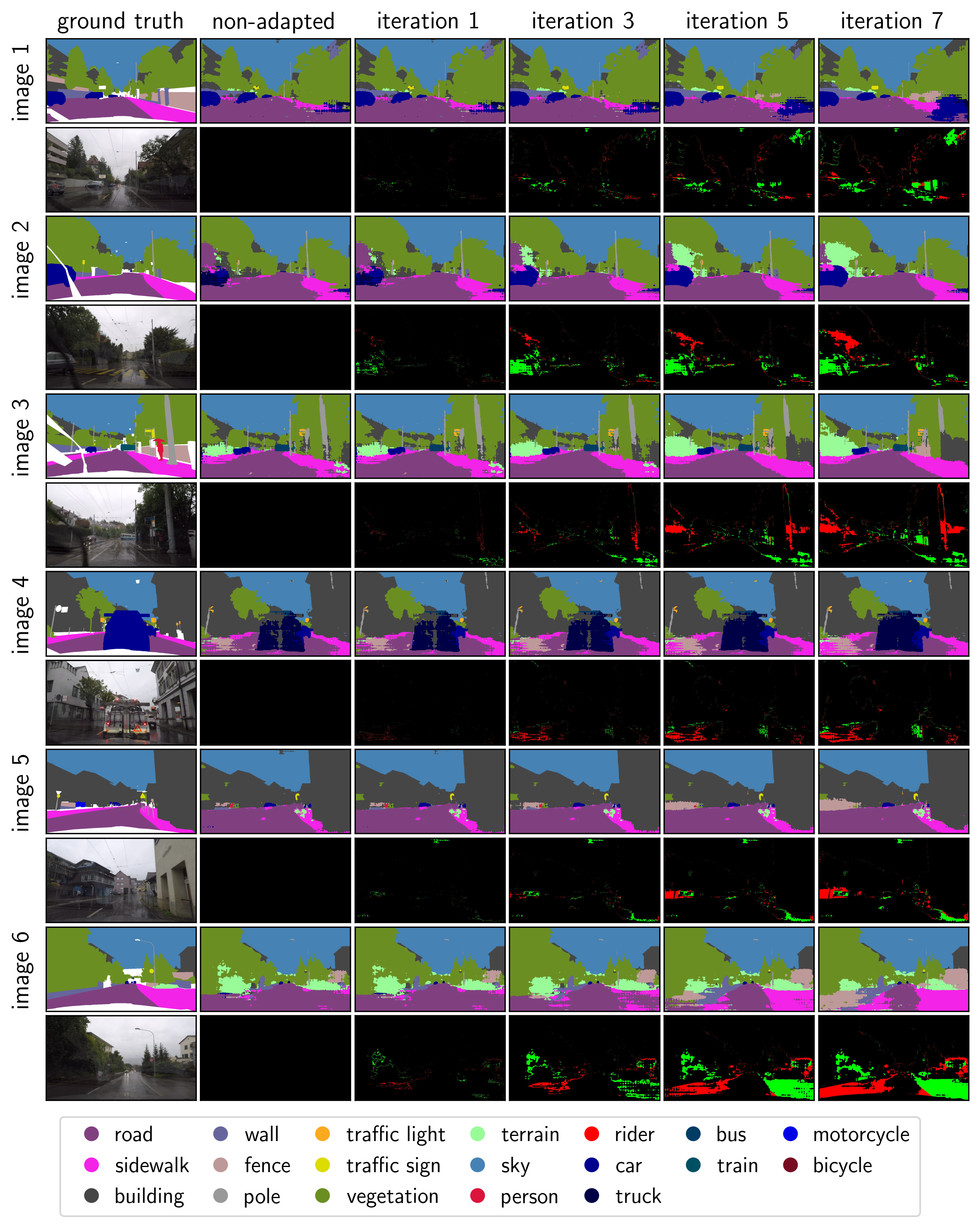
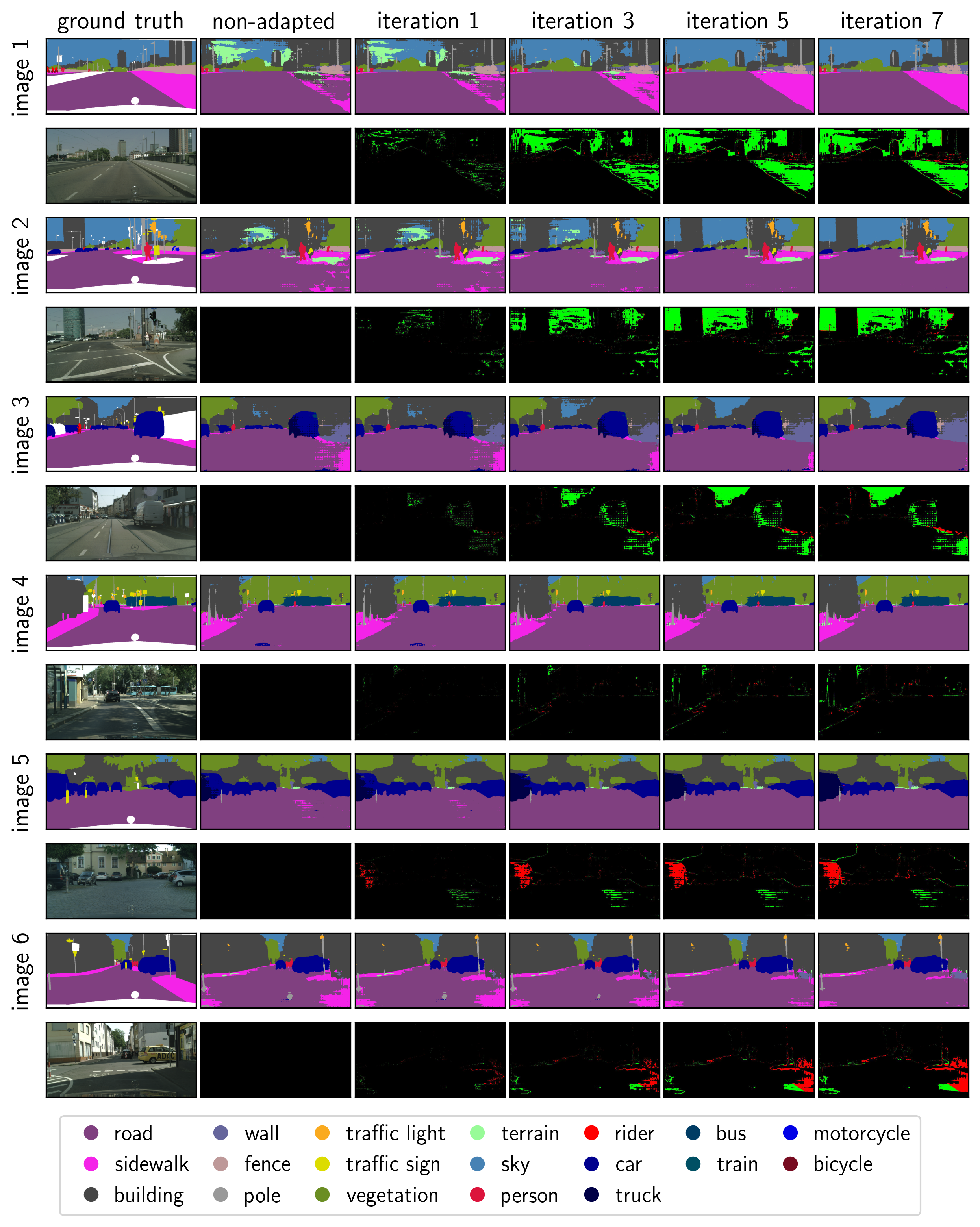
Visualization on test datasets This part presents the visualizations of the Ref TTA method on the test datasets. The Ref method was selected because among the best performing methods, it is the most novel in the image segmentation setup and has shown particularly strong performance on images most severely impacted by domain shift. The visualizations can be found in Figure 17 (VOC), Figure 18 (ACDC-fog), Figure 19 (ACDC-night), Figure 20 (ACDC-snow), Figure 21 (ACDC-rain) and Figure 22 (Cityscapes).

References

- [1] N Romero Aquino, Matheus Gutoski, Leandro T Hattori, and Heitor S Lopes. The effect of data augmentation on the performance of convolutional neural networks. Braz. Soc. Comput. Intell, 2017.
- [2] Jimmy Lei Ba, Jamie Ryan Kiros, and Geoffrey E Hinton. Layer normalization. arXiv preprint arXiv:1607.06450, 2016.
- [3] Alexander Bartler, Andre Bühler, Felix Wiewel, Mario Döbler, and Bin Yang. Mt3: Meta test-time training for self-supervised test-time adaption. In International Conference on Artificial Intelligence and Statistics, pages 3080–3090. PMLR, 2022.
- [4] Dian Chen, Dequan Wang, Trevor Darrell, and Sayna Ebrahimi. Contrastive test-time adaptation. In Proceedings of the IEEE/CVF Conference on Computer Vision and Pattern Recognition, pages 295–305, 2022.
- [5] Marius Cordts, Mohamed Omran, Sebastian Ramos, Timo Rehfeld, Markus Enzweiler, Rodrigo Benenson, Uwe Franke, Stefan Roth, and Bernt Schiele. The cityscapes dataset for semantic urban scene understanding. In Proceedings of the IEEE conference on computer vision and pattern recognition, pages 3213–3223, 2016.
- [6] Mark Everingham, Luc Van Gool, Christopher KI Williams, John Winn, and Andrew Zisserman. The pascal visual object classes (voc) challenge. International journal of computer vision, 88:303–338, 2010.
- [7] Alain Fournier, Don Fussell, and Loren Carpenter. Computer rendering of stochastic models. Communications of the ACM, 25(6):371–384, 1982.
- [8] Yossi Gandelsman, Yu Sun, Xinlei Chen, and Alexei A Efros. Test-time training with masked autoencoders. arXiv preprint arXiv:2209.07522, 2022.
- [9] Yossi Gandelsman, Yu Sun, Xinlei Chen, and Alexei A Efros. Test-time training with masked autoencoders. arXiv preprint arXiv:2209.07522, 2022.
- [10] Ian J Goodfellow, Jonathon Shlens, and Christian Szegedy. Explaining and harnessing adversarial examples. arXiv preprint arXiv:1412.6572, 2014.
- [11] Yves Grandvalet and Yoshua Bengio. Semi-supervised learning by entropy minimization. Advances in neural information processing systems, 17, 2004.
- [12] Dan Hendrycks and Thomas Dietterich. Benchmarking neural network robustness to common corruptions and perturbations. Proceedings of the International Conference on Learning Representations, 2019.
- [13] Sergey Ioffe and Christian Szegedy. Batch normalization: Accelerating deep network training by reducing internal covariate shift. In International conference on machine learning, pages 448–456, 2015.
- [14] Sergey Ioffe and Christian Szegedy. Batch normalization: Accelerating deep network training by reducing internal covariate shift. In International conference on machine learning, pages 448–456. pmlr, 2015.
- [15] Neerav Karani, Ertunc Erdil, Krishna Chaitanya, and Ender Konukoglu. Test-time adaptable neural networks for robust medical image segmentation. Medical Image Analysis, 68:101907, 2021.
- [16] Ansh Khurana, Sujoy Paul, Piyush Rai, Soma Biswas, and Gaurav Aggarwal. SITA: Single Image Test-time Adaptation.
- [17] Alexey Kurakin, Ian J Goodfellow, and Samy Bengio. Adversarial examples in the physical world. In Artificial intelligence safety and security, pages 99–112. Chapman and Hall/CRC, 2018.
- [18] Dong-Hyun Lee et al. Pseudo-label: The simple and efficient semi-supervised learning method for deep neural networks. In Workshop on challenges in representation learning, ICML, volume 3, page 896, 2013.
- [19] Bo Li, Yezhen Wang, Tong Che, Shanghang Zhang, Sicheng Zhao, Pengfei Xu, Wei Zhou, Yoshua Bengio, and Kurt Keutzer. Rethinking distributional matching based domain adaptation. arXiv preprint arXiv:2006.13352, 2020.
- [20] Tsung-Yi Lin, Michael Maire, Serge Belongie, James Hays, Pietro Perona, Deva Ramanan, Piotr Dollár, and C Lawrence Zitnick. Microsoft coco: Common objects in context. In Computer Vision–ECCV 2014: 13th European Conference, Zurich, Switzerland, September 6-12, 2014, Proceedings, Part V 13, pages 740–755. Springer, 2014.
- [21] Yuejiang Liu, Parth Kothari, Bastien van Delft, Baptiste Bellot-Gurlet, Taylor Mordan, and Alexandre Alahi. Ttt++: When does self-supervised test-time training fail or thrive? Advances in Neural Information Processing Systems, 34:21808–21820, 2021.
- [22] Yuang Liu, Wei Zhang, and Jun Wang. Source-free domain adaptation for semantic segmentation. In Proceedings of the IEEE/CVF Conference on Computer Vision and Pattern Recognition, pages 1215–1224, 2021.
- [23] Ilya Loshchilov and Frank Hutter. Decoupled weight decay regularization. arXiv preprint arXiv:1711.05101, 2017.
- [24] Aleksander Madry, Aleksandar Makelov, Ludwig Schmidt, Dimitris Tsipras, and Adrian Vladu. Towards deep learning models resistant to adversarial attacks. arXiv preprint arXiv:1706.06083, 2017.
- [25] Zachary Nado, Shreyas Padhy, D Sculley, Alexander D’Amour, Balaji Lakshminarayanan, and Jasper Snoek. Evaluating prediction-time batch normalization for robustness under covariate shift. arXiv preprint arXiv:2006.10963, 2020.
- [26] Zachary Nado, Shreyas Padhy, D Sculley, Alexander D’Amour, Balaji Lakshminarayanan, and Jasper Snoek. Evaluating prediction-time batch normalization for robustness under covariate shift. arXiv preprint arXiv:2006.10963, 2020.
- [27] A Tuan Nguyen, Thanh Nguyen-Tang, Ser-Nam Lim, and Philip HS Torr. Tipi: Test time adaptation with transformation invariance.
- [28] A Tuan Nguyen, Thanh Nguyen-Tang, Ser-Nam Lim, and Philip H S Torr. TIPI: Test Time Adaptation with Transformation Invariance.
- [29] Viraj Prabhu, Shivam Khare, Deeksha Kartik, and Judy Hoffman. Augco: augmentation consistency-guided self-training for source-free domain adaptive semantic segmentation. arXiv preprint arXiv:2107.10140, 2021.
- [30] Stephan R Richter, Vibhav Vineet, Stefan Roth, and Vladlen Koltun. Playing for data: Ground truth from computer games. In Computer Vision–ECCV 2016: 14th European Conference, Amsterdam, The Netherlands, October 11-14, 2016, Proceedings, Part II 14, pages 102–118. Springer, 2016.
- [31] Adrian Lopez Rodriguez and Krystian Mikolajczyk. Domain adaptation for object detection via style consistency. arXiv preprint arXiv:1911.10033, 2019.
- [32] Olaf Ronneberger, Philipp Fischer, and Thomas Brox. U-net: Convolutional networks for biomedical image segmentation. In International Conference on Medical image computing and computer-assisted intervention, pages 234–241. Springer, 2015.
- [33] Kuniaki Saito, Donghyun Kim, Stan Sclaroff, Trevor Darrell, and Kate Saenko. Semi-supervised domain adaptation via minimax entropy. In Proceedings of the IEEE/CVF international conference on computer vision, pages 8050–8058, 2019.
- [34] Christos Sakaridis, Dengxin Dai, and Luc Van Gool. Acdc: The adverse conditions dataset with correspondences for semantic driving scene understanding. In Proceedings of the IEEE/CVF International Conference on Computer Vision, pages 10765–10775, 2021.
- [35] Steffen Schneider, Evgenia Rusak, Luisa Eck, Oliver Bringmann, Wieland Brendel, and Matthias Bethge. Improving robustness against common corruptions by covariate shift adaptation. Advances in Neural Information Processing Systems, 33:11539–11551, 2020.
- [36] Andreas Steiner, Alexander Kolesnikov, Xiaohua Zhai, Ross Wightman, Jakob Uszkoreit, and Lucas Beyer. How to train your vit? data, augmentation, and regularization in vision transformers. arXiv preprint arXiv:2106.10270, 2021.
- [37] Yu Sun, Xiaolong Wang, Zhuang Liu, John Miller, Alexei Efros, and Moritz Hardt. Test-time training with self-supervision for generalization under distribution shifts. In International conference on machine learning, pages 9229–9248. PMLR, 2020.
- [38] Mingxing Tan and Quoc Le. Efficientnet: Rethinking model scaling for convolutional neural networks. In International conference on machine learning, pages 6105–6114. PMLR, 2019.
- [39] Eric Tzeng, Judy Hoffman, Kate Saenko, and Trevor Darrell. Adversarial discriminative domain adaptation. In Proceedings of the IEEE conference on computer vision and pattern recognition, pages 7167–7176, 2017.
- [40] Gabriele Valvano, Andrea Leo, and Sotirios A Tsaftaris. Re-using adversarial mask discriminators for test-time training under distribution shifts. arXiv preprint arXiv:2108.11926, 2021.
- [41] Riccardo Volpi, Pau De Jorge, Diane Larlus, and Gabriela Csurka. On the road to online adaptation for semantic image segmentation. In Proceedings of the IEEE/CVF Conference on Computer Vision and Pattern Recognition, pages 19184–19195, 2022.
- [42] Dequan Wang, Evan Shelhamer, Shaoteng Liu, Bruno Olshausen, and Trevor Darrell. Tent: Fully test-time adaptation by entropy minimization. arXiv preprint arXiv:2006.10726, 2020.
- [43] Dequan Wang, Evan Shelhamer, Shaoteng Liu, Bruno Olshausen, and Trevor Darrell. Tent: Fully test-time adaptation by entropy minimization. arXiv preprint arXiv:2006.10726, 2020.
- [44] Qin Wang, Olga Fink, Luc Van Gool, and Dengxin Dai. Continual test-time domain adaptation. In Proceedings of the IEEE/CVF Conference on Computer Vision and Pattern Recognition, pages 7201–7211, 2022.
- [45] Renhao Wang, Yu Sun, Yossi Gandelsman, Xinlei Chen, Alexei A Efros, and Xiaolong Wang. Test-Time Training on Video Streams.
- [46] Ross Wightman. Pytorch image models. https://github.com/rwightman/pytorch-image-models, 2019.
- [47] Yue Zhang, Shun Miao, Tommaso Mansi, and Rui Liao. Task driven generative modeling for unsupervised domain adaptation: Application to x-ray image segmentation. In Medical Image Computing and Computer Assisted Intervention–MICCAI 2018: 21st International Conference, Granada, Spain, September 16-20, 2018, Proceedings, Part II, pages 599–607. Springer, 2018.