Mixing as a correlated aggregation process

Abstract

Mixing describes the process by which scalars, such as solute concentration or fluid temperature, evolve from an initial heterogeneous state to uniformity under the stirring action of a fluid flow. Mixing occurs initially through the formation of scalar lamellae as a result of fluid stretching and later by their coalescence due to molecular diffusion. Owing to the linearity of the advection-diffusion equation, scalar coalescence can be envisioned as an aggregation process. While random aggregation models have been shown to capture scalar mixing across a range of turbulent flows, we demonstrate here that they are not accurate for most chaotic flows. In particular, we show that the spatial distribution of the number of lamellae in aggregates is highly correlated with their elongation and is also influenced by the fractal geometry that arises from the chaotic flow. The presence of correlations makes mixing less efficient than a completely random aggregation process because lamellae with similar elongations and scalar levels tend to remain isolated from each other. Based on these observations, we propose a correlated aggregation framework that captures the asymptotic mixing dynamics of chaotic flows and predicts the evolution of the scalar pdf based on the flow stretching statistics. We show that correlated aggregation is uniquely determined by a single exponent which quantifies the effective number of random aggregation events, and is dependent on the fractal dimension of the flow. These findings expand aggregation theories to a larger class of systems, which have relevance to various fundamental and applied mixing problems.

1 Introduction

The mixing of solutes by the stirring action of heterogeneous velocity fields is ubiquitous to natural and industrial processes (Ottino, 1990; Le Borgne et al., 2013; Villermaux, 2019). The transport of a passive diffusive scalar in an incompressible velocity field $\bm{v}$ is governed by the conservation equation

$$\partial_{t}c+\bm{v}\bm{\nabla}c=\kappa\bm{\nabla}^{2}c,$$ (1)

with $c$ the scalar concentration and $\kappa$ the molecular diffusivity. Despite being fully linear, the interplay between advection and diffusion produces non-trivial mixing dynamics across a large spectrum of flows, including turbulent flows (Villermaux & Duplat, 2003a, 2006; Duplat & Villermaux, 2008a), porous media flows (Le Borgne et al., 2015; Lester et al., 2016; Heyman et al., 2020; Souzy et al., 2020; Heyman et al., 2021) and chaotic flows (Wonhas & Vassilicos, 2002; Fereday et al., 2002; Haynes & Vanneste, 2005).

As illustrated in Fig. 1a, an initial blob of scalar stirred in a two-dimensional chaotic flow, produces elongated scalar structures, called filaments or lamellae, whose lengths increase exponentially with time. Accordingly, their widths decay by compression until it equilibrates with diffusion at the Batchelor scale (Batchelor, 1959) $s_{B}\sim\sqrt{\kappa/\lambda}$, with $\lambda$ the mean stretching rate experienced by fluid elements along their trajectory—the so-called Lyapunov exponent. Once the lamellar width reaches $s_{B}$, the diffusive flux balances the compression rate, and irreversible mixing takes place. When filaments remain isolated from each other, it is possible (Meunier & Villermaux, 2010) to predict exactly the evolution of scalar concentration by quantifying their Lagrangian stretching history. However, material lines also bend due to the presence of second-order derivatives in the spatial field $\bm{v}$ (Tang & Boozer, 1996), creating folds (Fig. 1b). Fluid compression exponentially reduces the distances between folds, which creates a highly foliated structure at a later time (Fig. 1a). Individual filaments are thus no longer isolated, but start to coalesce at scales of the order of $s_{B}$, while the mixture keeps homogenising and its concentration tends to the mean $\langle c\rangle$. This so-called aggregation process (Villermaux & Duplat, 2003a) obeys two essential properties. First, filament positions tend to accumulate at infinitesimal scales due to exponential flow compression. Bundles of aggregated lamellae are thus formed by individual filaments sharing the same region of size $\sim s_{B}$. Second, the linearity of the advection-diffusion equation implies that scalar concentration fields can be decomposed into a sum of the concentration profiles of solitary lamellae  (Le Borgne et al., 2017). Considering a flow domain area $\mathcal{A}$, the aggregation regime is attained when the total length of lamellae is

$$L(t)s_{B}\gtrsim\mathcal{A},$$ (2)

Assuming a constant stretching rate $\gamma$, $L(t)=\ell_{0}\exp(\gamma t)$, the coalescence time $t_{c}$ at which Eq. 2 is first fulfilled is

$$t_{c}\sim\frac{1}{\gamma}\log\left(\frac{\mathcal{A}}{\ell_{0}s_{B}}\right).$$ (3)

The mean number of filaments in bundles is

$$n(t)\sim\frac{L(t)s_{B}}{\mathcal{A}},$$ (4)

and the scalar concentration $c$ in a bundle is formed by the superposition of $n$ elementary lamellar concentrations $\theta_{i}$ present inside a given bundle

$$c(t)\sim\sum_{i=1}^{n(t)}\theta_{i}(t).$$ (5)

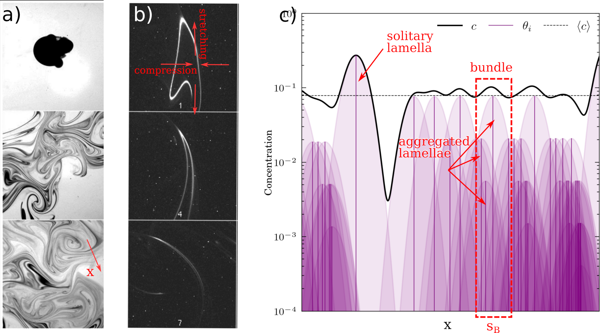
Figure 1: a. Mixing of a diffusive scalar by a random stirring protocol (time sequence top to bottom), evidencing the apparition of stretched scalar filaments (adapted from Villermaux (2012)). b. Blow up on the coalescence of neighbouring filaments under the action of compression (adapted from Duplat & Villermaux (2008a)) c. Concentration profile of a scalar field showing the coexistence of solitary filaments and bundles of filaments. The scalar concentration $c$ is obtained by the superposition of individual filamentary concentrations, which all have a Gaussian shape with maximum concentration $\theta_{i}$ and width $s_{B}$ (see Section 3.1).

Two scenarii have been proposed to describe the statistical properties of the sum (5): a fully random (Villermaux & Duplat, 2003b) and a fully correlated (Heyman et al., 2021) aggregation processes. These scenarii correspond to two caricatural routes towards homogeneity, described below.

The purely random scenario was proposed (Duplat & Villermaux, 2008b) to describe aggregation dynamics in scalar turbulence. It was therefore assumed that the stirring action of turbulent flows is sufficiently random for the aggregation of individual filaments to be decoupled from their individual stretching histories. The scalar concentration $c$ in a bundle can thus be formed by the sum of $n$ independent and identically distributed random variables, following the solitary filament concentration pdf. Under this assumption, the scalar concentration pdf, $P_{c}(c,t)$, results from the $n$-convolution of the isolated lamella concentration pdf $P_{\theta}(\theta,t)$, with the mean number of aggregations $n$ given by Eq. (4). If $P_{\theta}$ is exponential or gamma distributed, then $P_{c}$ is a gamma distributed

$$P_{c}(c)=\frac{n^{n}}{\Gamma(n)}\left(\frac{c}{\langle c\rangle}\right)^{n-1}\exp\left(-n\frac{c}{\langle c\rangle}\right)$$ (6)

Thus, the scalar variance decays as

$$\sigma^{2}_{c}=\frac{\langle c\rangle^{2}}{n}\sim 1/L(t).$$ (7)

Skewer lamella concentration distributions (e.g. log-normal pdf) do not produce gamma distributions when convolved $n$ times (Schwartz & Yeh, 1982), but the scalar variance still follows $1/L(t)$ asymptotically. For a uniform stretching rate, the random aggregation scenario thus predicts a variance decay equal to the pre-asymptotic regime of isolated strips (see Meunier & Villermaux (2010) and derivations in Appendix B). For random stretching rates, it predicts a faster decay compared to the pre-asymptotic regime (Fig. 2c). This is in contradiction with numerical computations of chaotic mixing that suggest the same decay exponent before and after aggregation time (Fereday et al., 2002; Tsang et al., 2005). For instance, a log-normal distribution of stretching rates of mean $\mu$ and variance $\sigma^{2}$ (with $\mu\geq\sigma^{2}$) yields $n\sim\exp((\mu+\sigma^{2}/2)t)$ and an asymptotic scalar decay exponent of $\mu+\sigma^{2}/2$, versus $\mu-\sigma^{2}/2$ for solitary strips (Meunier & Villermaux, 2010). The alternative model $n\sim\exp(\mu t)$ was also proposed (Villermaux & Duplat, 2006) to account for the fact that stretching fluctuations may weakly affect $n$. However, this scaling does not conserve the mean concentration and also overestimates the decay of scalar variance.

The opposite caricature is the fully correlated aggregation scenario, whereby lamella aggregate in the exact proportion of their elongation (Heyman et al., 2021). Correlation between aggregation and elongation occurs naturally in incompressible flows because lamella elongation $\rho$ is always balanced with transverse compression $1/\rho$ (Fig. 1b), which attracts neighbouring lamella and locally increases $n$. In this scenario, the weakly stretched regions of the flow have also experienced little compression, thus remaining isolated from the bulk. They are thus well described by the isolated lamellar theory. These poorly stretched lamellae bear typically high concentration levels, thus dominating scalar fluctuations. The correlated aggregation mechanism was first observed experimentally from the evolution of the concentration pdf of two dyes concentrations $c_{1}$ and $c_{2}$ in a chaotic mixer (Duplat et al., 2010). The authors showed that if the dyes were deposited inside a concentric annulus, the mean $c=(c_{1}+c_{2})/2$ would have the same pdf as the parts, $c_{1}$ and $c_{2}$. In other words, $c_{1}$ and $c_{2}$ are locally equal because they have experienced the same stretching history before aggregating. The evolution of the scalar pdf in a fully correlated regime can then be estimated as follows. If a bundle includes $n$ lamellae of the same concentration level $\theta$, Eq. (47) simplifies to $c\sim n\theta$. In the fully correlated scenario, $n$ is proportional to the filament elongation $\rho$,

$$n\approx 1+\rho/\rho_{c}$$ (8)

with $\rho_{c}=\mathcal{A}/(s_{B}\ell_{0})$, the mean elongation at coalescence time. In turn, the individual filament concentration follows $\theta=\theta_{0}s_{0}/s_{B}\rho^{-1}$ (see section 3.1) such that

$$c-\langle c\rangle\approx\frac{\theta_{0}s_{0}}{s_{B}}\rho^{-1},$$ (9)

where we identified the mean spatial concentration $\langle c\rangle=\theta_{0}\ell_{0}s_{0}/\mathcal{A}$. Thus, the pdf of the deviation from the mean $\tilde{c}=c-\langle c\rangle$ follows the pdf of $\rho^{-1}$, which is completely determined by the stretching statistics of flow (Fig. 2c). Since the is log-normal in random chaotic flows with mean $-\mu t$ and variance $\sigma^{2}t$, we expect similar statistics for $c-\langle c\rangle$. Note that highly elongated portions of the filament occupy the same area as weakly elongated ones. Thus, because aggregation is correlated, stretching statistics must be considered with respect to the initial filament state rather than the final one. The scalar decay exponent in the fully correlated scenario is thus very close to the one of solitary strips, thus explaining similarities between pre- and post-aggregation scalar decay exponents (Wonhas & Vassilicos, 2002; Tsang et al., 2005; Fereday et al., 2002). While accurately describing extremes, the fully correlated scenario causes an unrealistic peaking of the scalar pdf close to the mean (Fig. 2c), due to the complete absence of mechanisms to mix bundles of different $\rho$. This is in contradiction with the homogenising capacity of chaotic flows.

Hence, aggregation dynamics in chaotic flows likely lie between a fully random and a fully correlated scenario. The goal of this study is thus to uncover the statistical laws governing aggregation processes in chaotic flows. In particular, we describe the impact of stochastic aggregation on the spatial distribution of $n$ and $c$ and their moments. We focus on scalar aggregation in the so-called Batchelor regime (Haynes & Vanneste, 2005), for which the minimum scale of scalar fluctuation $s_{B}$ is much smaller than the smallest velocity correlation length scale, and for which no scalar gradients develop at large scales. Such regime is also qualified as “smooth” flows because velocity gradients remain relatively constant at the scale of $s_{B}$. This is in contrast to “rough” flows (e.g., turbulent flows at low Schmidt numbers) where the smaller flow scales lie below the Batchelor scale.

The paper is organised as follows. We first discuss the two main hypothesis proposed to describe lamella aggregation in heterogeneous flows (section 2). We then use chaotic flow simulations to derive a new correlated aggregation theory. In Section 3, we describe the fractal feature of material lines in heterogeneous chaotic flows and its link to the distribution of the number of aggregated lamellae. In Section 4, we investigate the properties of correlated aggregation. In Section 5, we derive a model for the aggregated scalar pdf.

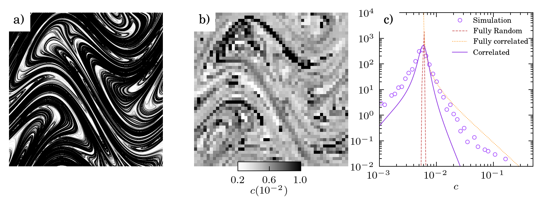
Figure 2: a) Geometry of material lines (lamellae) in the sine flow at time $t=12$ for $A=0.9$. b) Coarsened concentration field resulting from the sum of lamellar concentration in a neighbourhood of size $s_{B}$. c) Pdf of the coarsened scalar field and prediction of various models of aggregation.

2 Geometry of elongated material lines

2.1 Synthetic chaotic flows

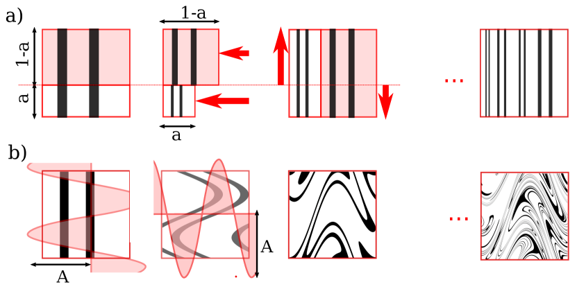
Figure 3: Transformations operated by a) the incompressible baker map with parameter $a$ and b) the sine flow with amplitude $A$ and random phases.

To understand the kinematics of aggregation, we first investigate the spatial geometry of advected fluid elements in two two-dimensional incompressible heterogeneous chaotic flows, namely the baker map and the sine flow (Fig. 3). These flows are sequential advective maps that have been widely used in the context of chaotic transport (Finn & Ott, 1988; Ott & Antonsen Jr, 1989; Tsang et al., 2005; Giona et al., 2001; Meunier & Villermaux, 2010, 2022) and are definedin the following.

In the incompressible baker map, fluid compression of factor $a\in[0,0.5]$ and $1-a$ first operates horizontally on the domain $y<a$ and $y>a$ respectively. Then vertical stretching occurs with a factor $1-a$ and $a$ in these two regions, preserving the total area (Fig. 3a). The transformation writes

$$x_{t+1} = \left\{\begin{array}[]{ll}ax_{t}&\text{ if }y_{t}<a\\ 1-(1-a)x_{t}&\text{ if }y_{t}>a\\ \end{array}\right.,$$

$$y_{t+1} = \left\{\begin{array}[]{ll}y_{t}/a&\text{ if }y_{t}<a\\ (1-y_{t})/(1-a)&\text{ if }y_{t}>a\\ \end{array}\right..$$

An advantage of the baker map is that purely vertical scalar patterns (for which $c(x,y)=f(x)$) remain one-dimensional after application of the map, thus simplifying the problem to a single dimension. This simplicity allows for the analytical derivation of many features of the map, as we will show later. Another advantage is that it is possible to explore a wide range of stretching heterogeneity by varying $a$ between 0 and 0.5. Indeed, the first two moments of stretching rate in the baker map are

$$\mu/t = -a\log(a)-(1-a)\log(1-a),$$ (12)

$$\sigma^{2}/t = a(1-a)(\log(1-a)-\log(a))^{2}.$$ (13)

Thus, for $a=0.01$, $\sigma^{2}/\mu=3.7$ while for $a=0.49$, $\sigma^{2}/\mu=5.7\cdot 10^{-4}$. It is important to note that this map involves discontinuous transformations, or “cuts”, that are absent in continuous flows such as turbulence but are common in flows through porous media (Lester et al., 2013).

In contrast, the sine flow is an alternation of random-phase horizontal and vertical sinusoidal velocity waves with amplitude $A$ and period $2\pi$ (Fig. 3b). The flow is periodic on the unit square $[0,1]\times[0,1]$ and it obeys for a given time period $t$

$$y_{t^{\prime}+\delta t} = y_{t^{\prime}}+A\delta t\left\{\begin{array}[]{ll}\sin(2\pi x_{t}^{\prime}+\phi_{t})&\text{ for }t<t^{\prime}<t+1/2,\\ 0&\text{ for }t+1/2<t^{\prime}<t+1\\ \end{array}\right.,$$

$$x_{t^{\prime}+\delta t} = x_{t^{\prime}}+A\delta t\left\{\begin{array}[]{ll}0&\text{ for }t<t^{\prime}<t+1/2,\\ \sin(2\pi y_{t}^{\prime}+\psi_{t})&\text{ for }t+1/2<t^{\prime}<t+1\\ \end{array}\right.,$$

where the amplitude $A$ is a positive constant and $\phi_{t},\psi_{t}$ are random phases that change at each time period $t$, and $\delta t=1/2$ the time step. The flow velocity having a single component, incompressibility is automatically ensured. Scalar transport is continuous and considered on a periodic domain $[0,1]\times[0,1]$. The stretching statistics of sine flows are described in Meunier & Villermaux (2022). As most random flows, the elongation of material lines in sine flows follows a log-normal distribution with a mean $\mu t$ and variance $\sigma^{2}t$ that depend on the amplitude $A$. The stretching heterogeneity is much less variable than in the baker map, with ratio $\sigma^{2}/\mu$ ranging from $1$ when $A\to 0$ to $\sigma^{2}/\mu\approx 0.6$ for $A=1.8$. In the following, we study the fractal geometry of advected material lines and their clustering in these chaotic flows.

The Lagrangian simulations consist in advecting a material filament in the flow field and follow its local elongation. The filament is defined by a series of consecutive points advected by the velocity field, linked by segments whose elongation is evolving due to velocity gradients. Segments that are highly elongated are refined by introducing intermediate points, in a similar manner as done by Meunier & Villermaux (2010). The elongated and folded filament (Fig. 2a) is tracked up to the advection time where $L=10^{7}\ell_{0}$, limit corresponding to our computer memory. Eulerian statistics, such as the local number of aggregated filaments, or their local mean elongation, are then computed by averaging Lagrangian variables on a regular grid (Fig. 2b) .

2.2 Fractal properties

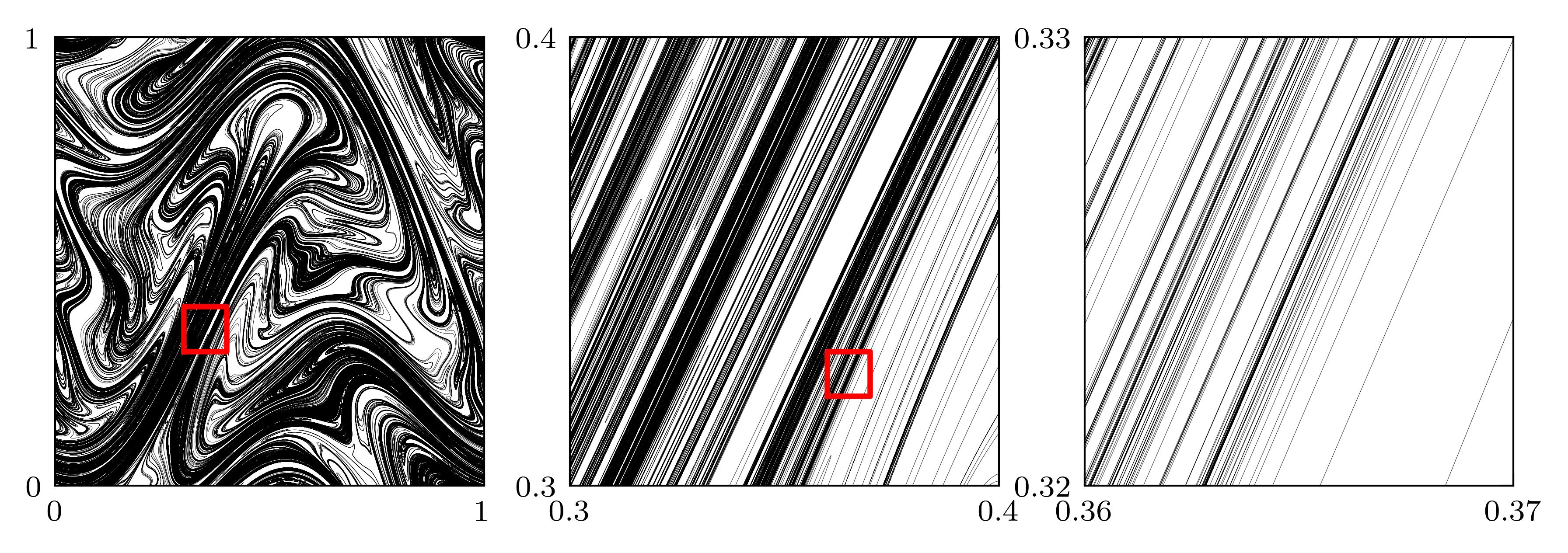
Figure 4: Fractal geometry of material material lines in (top) the sine flow ($A=0.8$) and (bottom) the baker map ($a=0.1$) observed at different scales

In incompressible flows, the stretching of material elements by velocity gradients is compensated by transverse compression. The compression causes distances between lamellar elements to decrease exponentially over time. Smaller and smaller scales are thus continuously produced by flow compression. Furthermore, in smooth chaotic flows, the typical scale of variation of velocity gradients is fixed and produces a heterogeneous stretching field for material lines. Dense (black) or diluted (white) regions of material lines are thus created at large scale in the chaotic flow (Fig. 4). Such heterogeneous structures then cascade to smaller scales under the action of net compression, thus creating a fractal set of one-dimensional objects (lines) clustered around their transverse direction. In two-dimensional incompressible flows, the Haussdorf dimension of this fractal set is necessarily $D_{0}=2$, as per the Kaplan-York result (Farmer et al., 1983). Higher dimensions can be smaller than 2 if stretching is heterogeneous. To illustrate this, let us define a normalised measure $p_{k}$ with $k=1\cdots N$ defining a regular grid of bin size $\epsilon=\mathcal{L}/N$, with $\mathcal{L}$ the system size. For instance, $p_{k}$ may be defined as the local density of lamella in the bin, e.g. $p_{k}=n_{k}/n$ where n is the total number of lamella. Since concentration levels of lamellae are additive, $p_{k}$ can be equivalently defined as the sum of lamella concentrations in one bin. The fractal dimension of order $q$ of the measure $p$ is then obtained with Grassberger (1983):

$$D_{q}-1=\lim_{\epsilon\to 0}\frac{1}{q-1}\frac{\log I_{q}(\epsilon)}{\log\epsilon},\quad I_{q}(\epsilon)\equiv\sum_{k}^{N=\mathcal{L}/\epsilon}p_{k}^{q},$$ (16)

where the subtraction of 1 on the left hand side accounts for the clustering of one-dimensional structures (lamellae) in a two-dimensional domain. This definition implies the following spatial scaling of the integral of the measure:

$$I_{q}(\epsilon)\sim\epsilon^{(q-1)(D_{q}-1)}.$$ (17)

In simple flows such as the baker map, $D_{q}$ can be obtained (Finn & Ott, 1988) by observing the similarity properties of the map, which transfer at small scales the heterogeneity of the measure produced at large scales by a single operation of the map. Characterising the result of one elementary operation of map on the measure thus also informs on the spectrum of fractal dimensions. In the following, we derive this spectrum for the baker map (see also Finn & Ott (1988)).

We consider the measure of the local number of lamella in bin $k$, $p_{k}=n_{k}/n$. As shown in Fig. 3a, an operation of the baker map doubles the total number of these lamellae, while maintaining the same local distribution of lamellae on smaller bins of sizes $a\epsilon$ for $x<a$ and $(1-a)\epsilon$ for $x>a$. The integral of the measure can then be computed by summing its value on the two replicates created by the map,

$$I_{q}(\epsilon)=I_{q,a}(\epsilon)+I_{q,1-a}(\epsilon).$$ (18)

We observe that

$$I_{q,a}(a\epsilon)=I_{q,1-a}((1-a)\epsilon)=\sum^{N=1/\epsilon}_{k}\left(\frac{p_{k}}{2}\right)^{q},$$ (19)

where the factor $1/2$ comes from the normalisation of the measure due to the doubling of $n$. Thus

$$I_{q,a}(\epsilon)=I_{q}(\epsilon/a)2^{-q}\mbox{ and }I_{q,1-a}(\epsilon)=I_{q}(\epsilon/(1-a))2^{-q}.$$ (20)

Replacing the last expression in (18) yields

$$I_{q}(\epsilon)=2^{-q}\epsilon^{(q-1)D_{q}}\left({a}^{-(q-1)(D_{q}-1)}+(1-a)^{-(q-1)(D_{q}-1)}\right)$$ (21)

Using the scaling $I_{q}(\epsilon)\sim\epsilon^{(q-1)D_{q}}$, thus provide a transcendental equation for $D_{q}$ independently of $\epsilon$:

$$2^{q}=\left({a}^{-(q-1)(D_{q}-1)}+(1-a)^{-(q-1)(D_{q}-1)}\right),$$ (22)

the solution of which is explicit for $q=0$ and $q=1$:

$$D_{0}=2,\quad D_{1}=1+\frac{2\log 2}{\log(a^{-1}+(1-a)^{-1})}.$$ (23)

Note that the solution for $q=1$ is obtained with Bernouilli’s rule by differentiating (22) with respect to $q$, and taking the limit $q\to 1$.

For random flows such as the sine flow, Ott & Antonsen Jr (1989) argue that there exists a general relationship between stretching rate statistics and fractal dimensions as $D_{q}=f_{q}(\sigma^{2},\mu)$, although a closed-form solution is not always trivial as for the baker map. We show in Fig. 5 that the ratio $\sigma^{2}/\mu$ is directly related to the fractal dimension $D_{1}$. This suggests that the fractal aggregation of material lines results from the large-scale heterogeneity of stretching rates. Since the flow is smooth, the heterogeneity created at large scales cascades to smaller scales, conserving its geometrical structure and creating a fractal geometry.

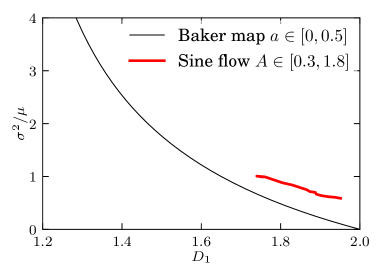
Figure 5: Relation between stretching rate mean $\mu$ and variance $\sigma^{2}$ and fractal dimension $D_{1}$ in the baker map and sine flow with varying parameters $a$ and $A$.

As suggested by Figure. 5, the function $f_{1}$ is different for baker map and the sine flow. Indeed, the ratio $\sigma^{2}/\mu$ tends to a positive constant in the sine flow when $A\to\infty$, while $\sigma^{2}/\mu\to 0$ in the baker map when $a\o 0.5$. This finite limit comes from the fact that the sine flow is a continuous transformation with no cutting and thus does not tend to a uniform stretching rate. In the contrary, when $A\to 0$, $\sigma^{2}/\mu\to 1$ which is a maximum bound for the ratio in the sine flow (Meunier & Villermaux, 2022), thus limiting the possible range of fractal dimensions produced by continuous chaotic flows, compared to discontinuous maps.

2.3 Spatial distribution of $n$

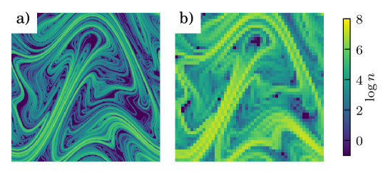
Figure 6: Numerical simulations showing the spatial distribution of the number of lamella $n$ in bundles in the sine flow ($A=0.5$) at two aggregation scales, $s_{B}=1/200$ (a) and $s_{B}=1/50$ (b).

The spatial distribution of the number of elements per bundle $n$ (Fig. 6) can be obtained as follows. Comparing the mean area occupied by a filament of length $L(t)$ and width $s_{B}$ to the domain surface $\mathcal{A}$, we get an estimate of the mean number of lamellae $\mu_{n}$ in bundles

$$\mu_{n}\sim L(t)s_{B}/\mathcal{A}.$$ (24)

Higher moments can be obtained from a study of the fractal structure of material lines. To this end, we consider the spatial measure corresponding to the local number of lamellae in each bundle:

$$p_{k}\equiv\frac{n_{k}}{\sum_{k}n_{k}}$$ (25)

The Renyi definition (Grassberger, 1983) of the fractal dimension of order 2 of this measure is

$$D_{2}-1\approx\frac{\log\sum_{k}p_{k}^{2}}{\log s_{B}},$$ (26)

when $s_{B}\to 0$. Replacing Eq. (25) in the last expression provides

$$\sum_{k}\left(\frac{n_{k}}{\sum_{k}n_{k}}\right)^{2}=s_{B}^{D_{2}-1}.$$ (27)

Since $\sum_{k}n_{k}=N\mu_{n}$ we have

$$\sum_{i}\left(\frac{n_{k}}{\sum_{k}n_{k}}\right)^{2}=\frac{1}{N}\left\langle\left({n}/{\mu_{n}}\right)^{2}\right\rangle,$$ (28)

with $N\approx\sqrt{\mathcal{A}}/s_{B}$ the number of bundles in the flow domain. Since

$$\sigma^{2}_{n/\mu_{n}}=\left\langle\left(n/\mu_{n}\right)^{2}\right\rangle-\left\langle n/\mu_{n}\right\rangle^{2},$$ (29)

then,

$$\sigma^{2}_{n/\mu_{n}}=\sqrt{\mathcal{A}}s_{B}^{D_{2}-2}-1.$$ (30)

Thus the variance of $n/\mu_{n}$ reaches a constant at asymptotic times, which is given by the fractal dimension of order 2. The spatial variance of $n$ is then

$$\sigma^{2}_{n}=\mu_{n}^{2}\left(\sqrt{\mathcal{A}}s_{B}^{D_{2}-2}-1\right)$$ (31)

The predictions of Eqs. (24)-(31) are plotted against time in Fig. 7 showing good agreement with simulations for a large range of Batchelor scales $s_{B}$ and flow heterogeneity, characterized by the parameters $a$ for the Baker map and $A$ for the sine flow.

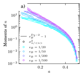
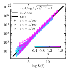
Figure 7: a) Scaling of the spatial variance of $\log n$ as a function of $a$ in the baker map and theoretical prediction, Eq. (30). b) First two moments of $P_{n}$ through time compared to theoretical predictions, Eqs. (24) and (31) in the baker map and c) in the sine flow. In these flows, the surface and length of the flow domain are equal to 1.

The pdf of lamella aggregation number $P_{n}(n)$ closely follows a Gamma distribution for all simulated data in both baker and sine flow over a large range of time and fractal dimensions (Fig. 8):

$$P_{n}(n)=\frac{1}{\Gamma(k_{n})\theta^{k}_{n}}n^{k_{n}-1}\exp(-n/\theta_{n}),$$ (32)

with $n\geq 0$ and $k_{n},\theta_{n}$ defined by the moments of the distribution of n :

$$k_{n} = \left(\sqrt{\mathcal{A}}s_{B}^{D_{2}-2}-1\right)^{-1},$$ (33)

$$\theta_{n} = \mu_{n}(t)\left(\sqrt{\mathcal{A}}s_{B}^{D_{2}-2}-1\right),$$ (34)

with $\mu_{n}=L(t)\mathcal{A}/s_{B}$. Note that the gamma distribution yields a power law distribution at small $n$ with exponent $k_{n}$ going from zero to infinity with increasing $D_{1}$. It may thus not have finite variance if $k_{n}>1$, that is for small $D_{2}$ (large heterogeneity). In that case, all the probability is concentrated to low values of $n$, thus in non-aggregated regions of the flow. In practice, we impose $n\geq 1$ to ensure integrability of moments.

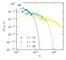
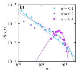
Figure 8: $P(n,t)$ for the baker map and sine flow for $s_{B}=1/100$. Solid lines stand for the gamma pdf with theoretical moments given by Eq. (34) and dots stand for numerical simulations. a) baker map $a=0.3$ and variable $t$. b) baker map for $t=20$ and variable $a$. c) sine flow for $s_{B}=1/100$ and $A=0.4$.

3 Lamellar concentrations in bundles

Figure 9: Simulation of aggregation statistics in baker map ($a=0.3$) and sine flow ($A=0.5$) for $s_{B}=1/50$ : .1 number of lamella $n$ in bundles, .2 mean of log-elongation in bundles and .3 sum of lamellar concentrations in bundles.

The linearity of the advection diffusion operator (1) offers the possibility to decompose the scalar mixing problem into a sum of various initial value problems, similar to Green’s functions. Thus, the asymptotic scalar concentration field can be envisioned as a local summation of solitary diffusive lamellae (Fig. 1), that are present in the same region at the same time. In the following, we recall the Lagrangian description of these solitary diffusive lamella.

3.1 The solitary lamella theory

Solitary lamellae are thin and elongated scalar structures that spontaneously form under the stirring action of a flow (Fig. 1). An analytical prediction of the temporal evolution of these quasi one-dimensional structures can be derived in a Lagrangian frame with a coordinate system $(x,y)$ advected with the flow and aligned with the directions of compression ($x$) and elongation ($y$) (Ranz, 1979; Villermaux, 2019). Because of their elongated shape, the concentration of lamellae is almost constant in the $y$ direction. Thus, $\partial_{y}c$ is negligible compared to $\partial_{x}c$, and the two-dimensional advection-diffusion problem (1) simplifies to a one-dimensional advection-diffusion equation

$$\partial_{t}c+u(x)\partial_{x}c=\kappa\partial^{2}_{x}c,$$ (35)

with $u=-x\gamma(t)$ the velocity at which solute particles are compressed in the direction $x$ and $\gamma(t)\geq 0$ the stretching rate. Owing to flow incompressibility, the stretching rate $\gamma(t)$ in the $y$-direction leads to a compression rate $-\gamma(t)$ in the $x$-direction. This approximation is valid when the characteristic compression time $\gamma^{-1}$ is smaller than the characteristic diffusion time $s_{0}^{2}/D$, where $s_{0}^{2}$ is the initial lamella width, which is for $\text{Pe}_{0}=\gamma s_{0}^{2}/\kappa>1$ (Villermaux, 2019). Following Ranz (1979), we define a dimensionless rescaled time

$$\tau=\frac{\kappa}{s_{0}^{2}}\int_{0}^{t}\rho(r)^{2}\text{d}r.$$ (36)

where $\rho(t)=\exp(\int_{0}^{t}\gamma(t^{\prime})\text{d}t^{\prime})$ is the lamella elongation, and a dimensionless rescaled space $\xi=x\rho/s_{0}$. In these rescaled coordinates, Eq. (35) transforms to a simple diffusion equation

$$\partial_{\tau}c=\partial^{2}_{\xi}c,$$ (37)

For a Gaussian initial condition $c(\xi,0)=\theta_{0}\exp(-\xi^{2})$, the solution is

$$c(\xi,\tau)=\frac{\theta_{0}}{\sqrt{1+4\tau}}\exp(-(\xi/\sqrt{1+4\tau})^{2}).$$ (38)

In the Lagrangian coordinate system $(x,y)$, the lamella scalar concentration follows

$$\Theta(x,t)=\theta(t)\exp(-(x/s(t))^{2})$$ (39)

where $\theta$ is the maximum concentration of the lamella, defined by

$$\theta=\frac{\theta_{0}}{\sqrt{1+4\tau}},$$ (40)

and $s$ the lamella width, following

$$s=\frac{s_{0}\sqrt{1+4\tau}}{\rho}.$$ (41)

Note that the mass in a given cross-section

$$m=\sqrt{\pi}\theta s=\sqrt{\pi}\theta_{0}s_{0}\rho^{-1}$$ (42)

is independent of the stretching history $\tau$, but depends only on the final elongation state. Multiplying by the lamella elongation recovers mass conservation.

In heterogeneous chaotic flows, we expect the Lagrangian elongation of lamellae $\rho$ to be a random variable. In Appendix A, we recall basic results concerning the statistical behaviour of $\rho$ in the sine flow and the baker map. The statistics of $\tau$, $\theta$ and $s$ can be further derived from the statistics of $\rho$. In chaotic flows, elongation increases exponentially fast ($\rho(t)=e^{\gamma(t)t}$) so that the last elongation value $\rho(t)$ has a predominant weight in the stochastic integral (36). An approximation of the statistics of $\tau$ was proposed (Meunier & Villermaux, 2010; Lester et al., 2016) as

$$\tau\approx\frac{\kappa}{2s_{0}^{2}}\frac{t}{\log\rho}(\rho^{2}-1).$$ (43)

When $t\to\infty$,

$$\tau\to\frac{\kappa}{2\lambda s_{0}^{2}}\rho^{2}=\frac{1}{4}\left(\frac{s_{B}}{s_{0}}\rho\right)^{2},$$ (44)

with $s_{B}=\sqrt{2\kappa/\lambda}$, the Batchelor scale. Thus,

$$\theta\to\frac{\theta_{0}s_{0}}{s_{B}}\rho^{-1}$$ (45)

and

$$s\to s_{B}.$$ (46)

3.2 Aggregated scalar level

After describing how solitary lamellae evolve in a chaotically stirred flow, we may now use the linear property of the advection-diffusion operator to obtain a description of the full scalar concentration field (Fig. 1). Indeed, the superposition of the concentration profiles (39) of solitary lamella allows reconstructing the aggregated scalar field. This property identity has been used to numerically retrieve scalar fields at large Péclet numbers  (Meunier & Villermaux, 2010).

To extract theoretical insights from this superposition process, we assume that at a later time, all lamellae reach the Batchelor scale and that their mass (Eq. (42)) can be homogeneously distributed inside a region of size $\sim s_{B}$. We also use this continuum scale as the typical coarsening scale for aggregation (Fig. 2b). Note that the theoretical results presented in the following are not sensitive to the precise choice of the aggregation scale, which can be as well defined as a multiple of the Batchelor scale. Consider a box of width $s_{B}$ centred in the position $\bm{x}$, the aggregated concentration level in this box can be constructed from the sum of the masses $m_{i}$ of the $n(\bm{x})$ individual lamellae present in this box

$$c(\bm{x})\approx\frac{1}{s_{B}}\sum_{i=1}^{n(\bm{x})}m_{i}=\frac{\sqrt{\pi}\theta_{0}s_{0}}{s_{B}}\sum_{i=1}^{n(\bm{x})}\rho^{-1}_{i}.$$ (47)

where we used Eq. (42) for the evolution of the solute mass carried by an individual lamella at a given location. Eq. (47) forms the base of the statistical description of aggregated concentration in chaotic flows. To simplify notations, we drop in the following the dependency on $\bm{x}$ of both $n$ and $c$, and consider these as random variables of space. It is tempting to deduce the statistical moments of $c$ with the similar scaling arguments as the ones used for $n$ (see Section 2.2). However, in contrast to $n$, $c$ is essentially non-fractal. Let us define the local measure

$$p_{k}=\frac{c_{k}}{\sum_{i=1}^{N}c_{i}}=\frac{\sum_{i=1}^{n_{k}}1/\rho_{i}}{\alpha},$$ (48)

where the normalising factor is

$$\alpha=\sum_{k}\sum_{i=1}^{n_{k}}1/\rho_{i}=L(t)\mu_{1/\rho,L},$$ (49)

with $\mu_{1/\rho,L}$ the mean of $1/\rho$ sampled along the filament’s length $L$. Taking the log-normal approximation for $\rho$ (see Appendix A),

$$\mu_{1/\rho,L} = e^{-(\mu+\sigma^{2})t+\sigma^{2}t/2},$$ (50)

$$L = \ell_{0}e^{(\mu+\sigma^{2}/2)t},$$ (51)

such that the normalisation factor is a time-independent constant. The dependence of $\langle p_{k}^{q}\rangle$ with scale can be derived analytically in simple map such as the baker map. Applying a similar procedure as described in Eq. (18), we find that

$$I_{q}=a^{q}I_{q}(\epsilon/a)+(1-a)^{q}I_{q}(\epsilon/(1-a))$$ (52)

such that

$$1=a^{(D_{q}-1)}+(1-a)^{(D_{q}-1)}.$$ (53)

Thus $D_{q}=2$ for all $q$, meaning that the aggregated concentration field is a non-fractal quantity. This result can also be intuitively understood as follows. Since aggregation is correlated, $1/n\sim 1/\rho$, so that both the number of lamellae in bundles $n$ and their mean elongation $\rho$ have similar fractal properties. Thus, the ratio $c\sim n/\rho$ is likely to be scale invariant. The fact that $D_{q}=2$ for all $q$ also means that scalar concentration ultimately tends to a dense and homogeneous field, in agreement with the mixing property of chaotic flows. The Renyi definition of the fractal dimension (Grassberger, 1983) for the measure defined in Eq. (48) reads

$$\frac{\sum_{k=1}^{N}c_{k}^{q}}{\left(\sum_{k=1}^{N}c_{k}\right)^{q}}=s_{B}^{(D_{q}-1)}=s_{B},$$ (54)

since $D_{q}=2$. Since $\sum_{k=1}^{N}c_{i}\to N\mu_{c}$, with $N=\sqrt{\mathcal{A}}/s_{B}$, we have

$$\langle(c/\mu_{c})^{q}\rangle\sim\sqrt{\mathcal{A}}s_{B}^{2-q}.$$ (55)

In particular, the second moment of $c$ ($q=2$) shows scale independence, e.g., $\langle(c/\mu_{c})^{2}\rangle\sim s_{B}^{0}$. Thus, the spatial fluctuations of $c$ are insensitive to Péclet number. To quantify these fluctuations and their temporal evolution, we must take a deeper look into the local distribution of lamellar elongations in bundles, their moments, and their relation to the bundle size.

3.3 Local correlations between $n$ and $\rho$

Figure 10: Joint pdf (gray scale) of the number of lamellae in a bundle of size $s_{B}=1/200$ and (1) their mean inverse elongation (2) and their mean log-elongation for (a.) baker map ($a=0.1,t=24,D_{1}=1.57$) and (b.) sine flow ($A=0.8$, $t=10$, $D_{1}=1.74$). The theoretical scaling of the measure (1) and (2), given by Eq. (57) and (59) respectively, are plotted as a continuous red lines with the slope indicated in the legend. Dashed red lines are guides to the eyes.

In contrast to the bundle size $n$, the scale independence of the aggregated concentration levels $c$ precludes describing the decay of scalar variance from the fractal geometry created by the chaotic flow. However, we will show that the fractal dimension still plays a role in determining the correlations between the bundle size $n$ and the local moments of lamella elongations in these bundles. To this end, we define the conditional averaging operator acting in lamellae located in the local neighbourhood of size $s_{B}$ by

$$\langle X|n\rangle=\frac{1}{n}\sum_{i=1}^{n}X_{i},$$ (56)

where $X$ is a Lagrangian variable transported by lamellae and $n$ is the number of lamellae aggregated in the bundle. The remainder of this Section is dedicated to uncovering the behaviour of conditional moments of elongation knowing $n$ (e.g. $\langle\rho^{-q}|n\rangle$). Section 4 will then be dedicated to deriving unconditional probabilities by averaging on the distribution of $n$.

We plot in Fig. 10 the joint probability $P(n(\bm{x}),\langle X|n\rangle)$ obtained in the baker map and the sine flow for $X=\rho^{-1}$ and $X=\log\rho$, the inverse of elongation and the log-elongation of lamella respectively. Fig. 10 suggests that the following scaling holds in both flows:

$$\log n\sim-\log\langle\rho^{-1}|n\rangle,$$ (57)

which confirms the strong correlation between the number of lamellae in aggregates and their elongation. For large time, $c$ must tend to the conserved average scalar concentration $c\to\langle c\rangle$. Thus we must have

$$n\sim 1/\langle\rho^{-1}|n\rangle,$$ (58)

a scaling that we confirm numerically (Fig. 10). In incompressible flows, the distance between lamellae $d$ is proportional to the amount of compression they have experienced, $\rho_{i}^{-1}$. Since the number of lamellae in a box of size $r$ is $n\sim 1/\langle d_{i}|n\rangle$, then, $n\sim 1/\langle\rho^{-1}|n\rangle$, which recovers the above result. Fig. 10 also suggests that

$$\log n\sim(D_{1}-1)\langle\log\rho|n\rangle,$$ (59)

where $D_{1}$ is the information dimension (Ott & Antonsen Jr, 1989) of the measure $n$, and is given by Eq. (23) for the baker map. Equation (59) can be derived exactly in the case of the baker map. Indeed, by the action of the map, the total number of lamellae increases as $\log n=t\log 2$ while the mean log-elongation of these lamellae is $\langle\log\rho\rangle=t(-\log a-\log(1-a))/2$ leading to a constant ratio

$$\frac{\log n}{\langle\log\rho\rangle}=\frac{2\log 2}{\log a+\log(1-a)},$$ (60)

which is exactly the value of $D_{1}-1$ (Eq. (23)). Assuming that the partition between $\log n$ and $\langle\log\rho\rangle$ is preserved at small scales in each bundle, we have

$$\log n=({D_{1}-1})(\langle\log{\rho}|n\rangle-\langle\log{\rho_{c}}|n\rangle)$$ (61)

with $\langle\log{\rho_{c}}|n\rangle$ a constant standing for the mean elongation at coalescence time ($n>1$). This thus proves Eq. (59) for the baker map. The constant $\langle\log{\rho_{c}}|n\rangle$ can be estimated by comparing the average surface $S=s_{B}\rho_{c}L_{0}$ occupied by the material line when it reaches the Batchelor scale $s_{B}$, with the available area $A$. The first aggregation event occurs when $S\approx A$, that is when $\rho_{c}\approx A/(s_{B}\ell_{0})$. Eq. (61) is verified for baker map and sine flow with various parameters $a$ and $A$, with $\langle\log{\rho_{c}}|n\rangle=-\log s_{B}$.

3.4 Distribution of $\log\rho$ in a bundle of size $n$

The two scaling laws $n\sim\langle\rho^{-1}|n\rangle$ and $\log n\sim(D_{1}-1)\langle\log\rho|n\rangle$ provide key information about the heterogeneity of lamella elongations inside bundles. Since the ensemble distribution of elongation $P_{\rho}(\rho)$ has a log-normal shape, we assume that the distribution of elongations inside bundles, denoted $P_{\rho|n}$, is also log-normally distributed. This implies that $\log\rho$ is normally distributed in bundles, with a mean

$$\mu_{\log\rho|n}\sim(D_{1}-1)^{-1}\log n.$$ (62)

Since $\log\langle\rho^{-1}|n\rangle=-\mu_{\log\rho|n}+\sigma^{2}_{\log\rho|n}/2\sim-\log n(\bm{x})$, the variance of log-elongation in bundles at large $n$ must be

$$\sigma^{2}_{\log\rho|n}\sim\frac{2(2-D_{1})}{D_{1}-1}\log n.$$ (63)

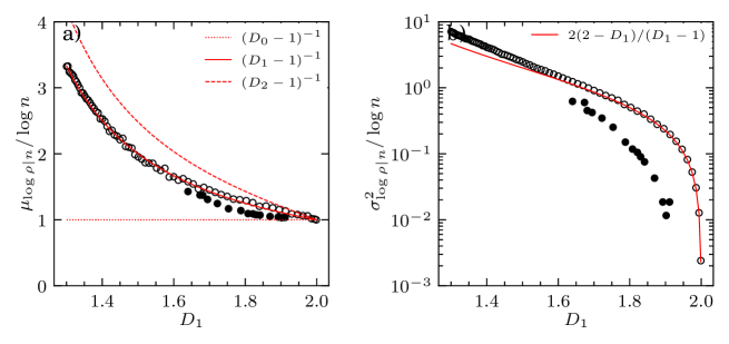
Figure 11: Scaling of the mean (a) and variance (b) of log-elongation in bundles as a function of the information dimension $D_{1}$. Circles stands for numerical simulations in baker maps (open circles) and sine flow (filled circles). Continuous lines stands for theoretical prediction of the mean (Eq. (62)) and variance (Eq. (63)). Dashed lines are plotted to compare the mean with fractal dimension of other order.

We report in Fig. 11 the simulated scaling $\mu_{\log\rho|n}/\log n$ and $\sigma^{2}_{\log\rho|n}/\log n)$ obtained asymptotically at large mixing times. When $D_{1}\to 2$, $\mu_{\log\rho|n}/\log n\to 1$ while $\sigma^{2}_{\log\rho|n}/\log n\to 0$, meaning that bundles are formed by lamella of identical elongations. In contrast, when $D_{1}\to 1$, both $\mu_{\log\rho|n}/\log n$ and $\sigma^{2}_{B}/\log n$ become infinite, while their ratio $\sigma^{2}_{\log\rho|n}/\mu_{\log\rho|n}=2(2-D_{1})\to 0.5$. This limit suggests that the aggregation of lamellae remains correlated to their average elongation, although a fixed amount of stretching variability arises in bundles. A good agreement is found between theoretical prediction (Eqs. (62)-(63)) and numerical simulations of aggregation in the baker map (Fig. 11). In contrast, the theory captures only qualitatively the behaviour of the random sine flow. This may be due to the continuity of the sine flow produces curved lamellar structures whose dimension is not exactly one-dimensional.

These results further invalidate the fully correlated aggregation hypothesis that assumes a uniform elongation in each bundle. Indeed, the stretching variability in bundles is directly linked to the heterogeneity of the chaotic flow, because of the intimate relationship existing between the fractal geometry of the chaotic attractor and the stretching statistics of fluid elements (Ott & Antonsen Jr, 1989). As such, it is impossible to have a single stretching rate per bundle as soon as the chaotic flow is heterogeneous and exhibits a distribution of stretching rates. The absence of stretching variability in bundles ($\sigma^{2}_{\log\rho|n}=0$) implies the uniformity of stretching at large scale ($\sigma^{2}_{\rho}=0$). This uniform case is reached when $D_{1}\to D_{0}=2$, for instance, in the baker map when $a\to 0.5$. In continuous flow maps such as the sine flow, regions of high and low stretching always coexist and $\sigma^{2}_{\log\rho|n}>0$.

3.5 Moments of $1/\rho$ in a bundle of size $n$

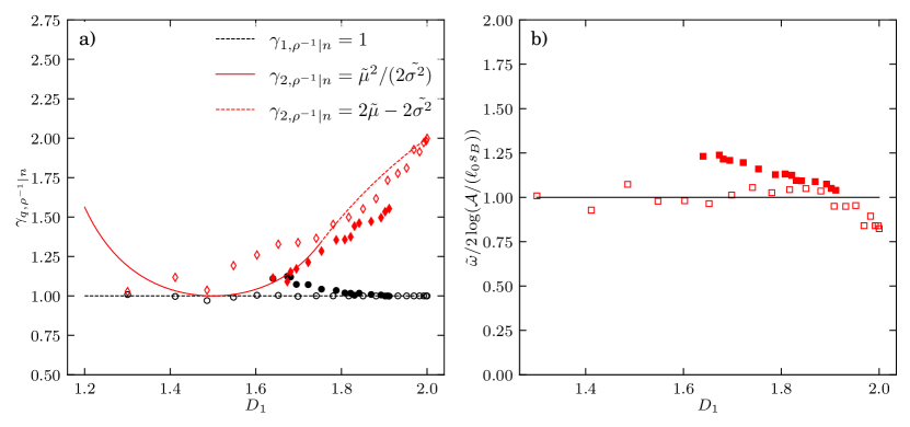
Figure 12: a) Scaling exponents of the $q$ lamellar concentration moments in bundles (Eq. (64)). Numerical estimates are plotted with symbols, red diamonds for $q=2$ and black circles for $q=1$. Unfilled and filled symbols represents simulations in baker map and sine flow respectively. Theoretical predictions (Eq. (70)) are represented by lines. b) Intercept $\tilde{\omega}$ of the scaling exponent of the $q$ lamellar concentration moments in bundles (Eq. (64)) in baker map (empty squares) and sine flow (filled squares) and theoretical prediction (line, Eq. (71)).

Having described the first two moments of the distribution of lamella elongation in bundles (Eqs (62)-(63)), we now assume that the distribution is of log-normal shape. This choice is justified by the fact that elongation is a multiplicative process, thus usually leading to lognormal distributions (Le Borgne et al., 2015; Souzy et al., 2020). This allows us to compute the scaling of the $q-$moments of lamella concentrations in bundles, $\theta|n$. Owing to Eq. (45), we have

$$\langle\theta^{q}|n\rangle \sim \langle\rho^{-q}|n\rangle$$ (64)

$$= \int_{1}^{\infty}\rho^{-q}P_{\rho|n}(\rho)\text{d}\rho$$

$$\approx \int_{1}^{\infty}e^{-(\log\rho-\mu_{\log\rho|n})^{2}/(2\sigma_{\log\rho|n}^{2})-q\log\rho}\text{d}\rho.$$

The minimum bound for the integral is taken at $\rho=1$ and not 0, taking into account the fact that lamellar structures cannot be compressed in their longitudinal direction. As a consequence, $P_{\rho|n}(\rho)$ is truncated for $\rho<1$. Denoting $\Lambda=\log\rho/\log n$, $\tilde{\mu}=\mu_{\log\rho|n}/\log n$ and $\tilde{\sigma}^{2}=\sigma_{\log\rho|n}^{2}/\log n$, this expression becomes

$$\langle\rho^{-q}|n\rangle\approx\int_{1}^{\infty}e^{H(\Lambda)\log n}\text{d}\rho,$$ (65)

with $H(\Lambda)=-(\Lambda-\tilde{\mu})^{2}/(2\tilde{\sigma}^{2})-q\Lambda$. For large $n$, the value of this integral tends to $e^{H(\Lambda^{*})\log n}$ where the $\Lambda^{*}$ is the value where $H$ takes a maximum, that is either at $\Lambda^{*}=\tilde{\mu}-q\tilde{\sigma}^{2}$ if $\tilde{\mu}-q\tilde{\sigma}^{2}>0$, or $\Lambda^{*}=0$ otherwise. Thus,

$$\log\langle\rho^{-q}|n\rangle \approx -({\gamma}_{q,\rho^{-1}|n}\log n+{\omega}_{q,\rho^{-1}|n})$$ (66)

with $$\left\{\begin{array}[]{ll}{\gamma}_{q,\rho^{-1}|n}=q\tilde{\mu}-q^{2}\tilde{\sigma}^{2}/2&\text{ if }\tilde{\mu}>q\tilde{\sigma}^{2},\\ {\gamma}_{q,\rho^{-1}|n}=\tilde{\mu}^{2}/(2\tilde{\sigma}^{2})&\text{ if }\tilde{\mu}\leq q\tilde{\sigma}^{2},\end{array}\right.$$ (69)

and ${\omega}_{q,\rho^{-1}|n}=q\log(\mathcal{A}/(s_{B}\ell_{0}))$ a constant. In particular, we are interested in the exponent $q=2$ which is useful to describe fluctuations around the mean. We have

$$\tilde{\gamma}\equiv{\gamma}_{2,\rho^{-1}|n}=\left\{\begin{array}[]{c}2\tilde{\mu}-2\tilde{\sigma}^{2}\text{ if }\tilde{\mu}>2\tilde{\sigma}^{2}\\ \tilde{\mu}^{2}/(2\tilde{\sigma}^{2})\text{ if }\tilde{\mu}\leq 2\tilde{\sigma}^{2}\end{array}\right..$$ (70)

The predicted dependence of $\tilde{\gamma}$ upon $D_{1}$ is reproduced in Fig. 12. $\tilde{\gamma}$ is bounded between 2 (for $D_{1}\to 2$) and 1 for $D_{1}\approx 1.5$. The prediction agrees reasonably well with numerical simulations of the baker and sine flows (Fig. 12). The slight discrepancies can be attributed to deviations from log-normally distributed elongation in bundles, as postulated before. We also verify numerically that $\tilde{\omega}\equiv\omega_{2,\rho^{-1}|n}$ is independent of $D_{1}$ (Fig. 12b). In Fig. 13, we verified that $\tilde{\gamma}$ is independent of the aggregation scale $s_{B}$. In contrast,

$$\tilde{\omega}\approx 2\log{\mathcal{A}/(l_{0}s_{B})},$$ (71)

is a sole function of the aggregation scale, independent of time and fractal dimension (Fig. 12.b).

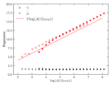
Figure 13: Dependence of $\tilde{\gamma}$ and $\tilde{\omega}$ with the Batchelor scale in simulations (dots) of the baker map (empty symbols $a=0.2$) and the sine flow (filled symbols $A=1.2$) and comparison to theoretical prediction (Eq. (71).

Having determined both the elongation statistics inside aggregates of size $n$ and the spatial distribution of $n$, we will deduce in the following section the statistics of aggregated scalar levels $c$.

4 Aggregated scalar concentrations

The scalar concentration of a bundle $c$ is formed by the superposition of the $n$ individual lamella contained in this bundle (Fig. 1), according to Eq. (5). The concentration of each individual lamella is a random variable; thus the superposition of these random variables is also a random variable, whose statistical properties are derived below.

4.1 Addition of scalar levels

We found that the moments of lamella elongation inside bundles of size $n$ follow:

$$\langle\rho^{-1}|n\rangle = \frac{s_{B}\ell_{0}}{\mathcal{A}}n^{-1}$$ (72)

$$\langle\rho^{-2}|n\rangle = \frac{(s_{B}\ell_{0})^{2}}{\mathcal{A}^{2}}n^{-\tilde{\gamma}}$$ (73)

with $\tilde{\gamma}\equiv\gamma_{2,\rho^{-1}|n}$ a flow-dependent exponent depending on $D_{1}$ and taking value between 1 and 2 (Fig. 12a). The variance of lamellar concentrations inside bundles thus follows:

$$\sigma^{2}_{\rho^{-1}|n} = \frac{(s_{B}\ell_{0})^{2}}{\mathcal{A}^{2}}\left(n^{-\tilde{\gamma}}-n^{-2}\right).$$ (74)

To relate the statistics of individual lamella concentrations inside bundles to the statistics of aggregate concentrations $c$, we assume that bundles are formed through Eq. (47) from a sum of independent and identically distributed random numbers. These random numbers must be picked from a random variable following the stretching statistics of lamellae among bundles of similar size $n$ rather than the statistics inside each of these bundles, as described above. However, as shown in Appendix C, such sampling effect do not play a role at large $n$, and we have

$$\sigma^{2}_{c|n}\approx n\left(\frac{\sqrt{\pi}\theta_{0}s_{0}}{s_{B}}\right)^{2}\sigma^{2}_{\rho^{-1}|n}=\frac{(\sqrt{\pi}\theta_{0}\ell_{0}s_{0})^{2}}{\mathcal{A}^{2}}\left(n^{1-\tilde{\gamma}}-n^{-1}\right),$$ (75)

When $n$ large, this expression further simplifies to

$$\sigma^{2}_{c|n}\sim n^{1-\tilde{\gamma}},$$ (76)

with $\tilde{\gamma}\in[1,2]$ given by Eq. 70. The mean concentration is conserved by the aggregation process, since

$$\langle c|n\rangle=n\cdot\frac{\sqrt{\pi}\theta_{0}s_{0}}{s_{B}}\langle\rho^{-1}|n\rangle=\frac{\sqrt{\pi}\theta_{0}\ell_{0}s_{0}}{\mathcal{A}}\equiv\langle c\rangle.$$ (77)

In Fig. 14, we compare the scaling of the second moment of $c|n$ with $n$ observed in numerical simulations to the prediction obtained with the independent assumption (Eq. (76)). The prediction is relatively accurate for the random sine flow, but largely underestimates the exponent for the deterministic baker map.

Indeed, the simplicity and regularity of the deterministic baker map makes bundles of similar size not statistically independent. While bundle concentration still results from the addition of variable lamellar concentrations, independent realisations of the summation are not achieved due to the deterministic nature of the baker map, the exact same lamellar geometrical patterns being repeated at a smaller and smaller scale. In the extreme case of a unique realization, the variance of the sum is exactly the variance of the random variable. Eq. (75), thus transforms into

$$\sigma^{2}_{c|n}\sim\sigma^{2}_{\rho^{-1},n}\sim n^{-\tilde{\gamma}},$$ (78)

a scaling that fits better the deterministic baker map simulations (Fig. 14). To summarise, the addition of lamellar concentration levels in a bundle yields a concentration whose deviation from the mean decays algebraically with the number of lamella in the bundle

$$\sigma^{2}_{c|n} \approx \frac{(\theta_{0}\ell_{0}s_{0})^{2}}{\mathcal{A}^{2}}n^{-\xi},$$ (79)

with $\xi=\tilde{\gamma}$ for purely deterministic flows (baker map) and $\xi=\tilde{\gamma}-1$ for random flows (sine flow). We call $\xi$ the correlation exponent, which can take values between 0 and 2 depending on the flow heterogeneity and randomness.

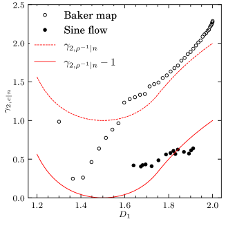
Figure 14: Scaling exponent $\xi$ (Eq. (79)) of the variance of bundle concentrations knowing $n$ estimated from simulations (dots) and theoretical predictions with the independent realisation hypothesis for the sine flow (dashed lines, $\xi=\tilde{\gamma}-1$, Eq. (76)) and baker map (continuous lines, $\xi=\tilde{\gamma}$, Eq. (78)).

4.2 Distribution of $c$

In Section 2, we derived the distribution of the number of lamella in bundles (Eq. (34)) and in Section 3, the scaling of the first two moments of aggregated concentration $c$ given the bundle size $n$ (Eq. (79)). With these elements, we can now express the unconditional pdf of scalar concentration $P_{c}$ via the sum

$$P_{c}(c)=\int_{n}\text{d}nP_{c|n}(c)P_{n}(n),$$ (80)

where $P_{c|n}$, the distribution of $c$ given the bundle size $n$, has to be specified. A possible choice for $P_{c|n}$ is the log-normal distribution, with parameters

$$\mu_{\log c|n} = \log\mu_{c|n}-\log(\sigma^{2}_{c|n}/\mu_{c|n}^{2}+1)/2$$ (81)

$$\sigma^{2}_{\log c|n} = \log(\sigma^{2}_{c|n}/\mu_{c|n}^{2}+1).$$ (82)

In Fig. 15, we plot the simulated distribution of aggregated concentration levels compared to the prediction Eq. (80) for the baker map and sine flow. The agreement is fair in the region near $\langle c\rangle$, but deviates for large $c$. Indeed, this corresponds to lamellae with weak aggregation for which $n\approx 1$. In this region, the solitary strip pdf $P_{\rho^{-1},L}$ describes well the tail of $P_{c}$ because such high concentration excursions are essentially supported by isolated lamellae, while the correlated aggregation model assumes $n\gg 1$. The presence of these weakly aggregated, high concentration levels is particularly evident at small $s_{B}$ (Fig. 15 (b)). The scalar concentration pdf is thus the combination of an aggregated core around the mean following Eq. (80) and tails following the isolated strip concentration pdf. In Figs. 2c and 16, we compare the correlated aggregation model with the random aggregation model where $\langle n\rangle\sim L(t)$ (Eq. (4)). The random aggregation assumption yields gamma pdfs (Eq. (6)) that are narrowing much faster than the simulated pdfs in the sine flow. In contrast, the fully correlated model captures well the tails of the pdf, but artificially peaks around the mean concentration. The correlated model is an intermediate scenario that captures both the tail and the center part of the pdf.

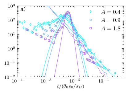
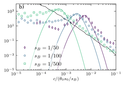
Figure 15: Distributions of aggregated scalar concentrations in the sine flow depending on a) the sine wave amplitude $A$ ($s_{B}=1/50$) and b) the aggregation scale $s_{B}$ ($A=0.9$). Dots stand for numerical simulations, continuous lines are the aggregation model (Eq.  (80)), and the dashed lines are the isolated strip prediction (Eq. (39)). Simulations are all taken at the time when the total filament length reaches $L=10^{7}\ell_{0}$.

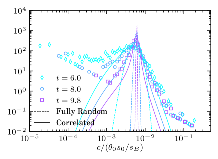
Figure 16: $P_{c}$ in sine flows at several times ($A=0.8,s_{B}=1/50$) (dots) compared with fully random aggregation (dashed lines, Eq. (6)) and correlated aggregation model (continuous lines, Eq. (80))

From pdf of aggregated scalar concentration, we now derive its moments. They are directly related to the pdf of $n$, since

$$\langle c\rangle = \int\text{d}c\sum_{n}cP(c|n)P(n)=\sum_{n}\langle c\rangle_{n}P(n)$$ (83)

$$= \frac{\theta_{0}\ell_{0}s_{0}}{\mathcal{A}}$$ (84)

and

$$\langle c^{2}\rangle = \int_{c}\text{d}c\int_{n}\text{d}n\,c^{2}P(c|n)P(n)=\int_{n}\,\text{d}n\langle c^{2}\rangle_{n}P(n)$$ (85)

$$= \frac{(\theta_{0}\ell_{0}s_{0})^{2}}{\mathcal{A}^{2}}(\langle n^{-\xi}\rangle_{n}+1).$$ (86)

Thus, the scalar variance is

$$\sigma^{2}_{c} = \frac{(\theta_{0}\ell_{0}s_{0})^{2}}{\mathcal{A}^{2}}\langle n^{-\xi}\rangle_{n}.$$ (87)

Note that $\langle n^{-\xi}\rangle$ is not defined for all $D_{1}$ when $k_{n}(D_{1})<\xi(D_{1})$, with $k_{n}$ the exponent of the gamma distribution chosen for the pdf of $n$ (Eq. (34)). This is because of the power law scaling of the gamma distribution near $n=0$, which may renders negative moments non-integrable. However, the $n\to 0$ limit is not relevant here because the flows are space-filling $(D_{0}=2)$ and asymptotically, $n\geq 1$. Thus, we cut the integral at $n=1$ to get

$$\langle n^{-\xi}\rangle_{n}\sim\left(\theta_{n}\right)^{-\text{min}(k_{n},\xi)}$$ (88)

An intuitive understanding of this equation can be formulated as follows. If the spatial heterogeneity of $n$ is moderate ($\xi<k_{n}$), the average of $n^{-\xi}$ is affected by all values of $n$ in the distribution. In contrast, if the heterogeneity is stronger ($\xi>k_{n}$), the probability of having low aggregation regions ($n\approx 1$) is high and controls the value of $\langle n^{-\xi}\rangle$. In that case, the average does not scale anymore with $\xi$, but rather with the parameter $k_{n}$, explaining the minimum exponent $\text{min}(k_{n},\xi)$. Combining Eq. (88) and Eq. (34) provides the asymptotic scalar variance decay as a function of the growth material length

$$\sigma^{2}_{c}(t)=\left(\frac{L(t)s_{B}(\sqrt{\mathcal{A}}s_{B}^{D_{2}-2}-1)}{\mathcal{A}}\right)^{-\text{min}(k_{n},\xi)}\sim L(t)^{-\text{min}(k_{n},\xi)},$$ (89)

where the growth of material length follows $L(t)=2^{t}$ in the baker map, and $L(t)=\exp((\mu+\sigma^{2}/2)t)$ in the sine flow. Thus, in a correlated aggregation scenario, the decay exponent of scalar variance is found to be a fraction of the growth exponent of material lines. In the sine flow, $k_{n}$ is generally larger than $\xi$ such that the scalar variance decay exponent is $\gamma_{c,2}=(\mu+\sigma^{2}/2)\xi$.

In Fig. 17.a, we compare the theoretical estimates of the scalar variance decay exponent $\gamma_{2,c}$ with simulations in the sine flow, showing relatively good agreement. Interestingly, the variance decay rate remains well predicted by the isolated strip model (see Appendix B) although its match with the full pdf is very poor except for large concentrations (Fig. 15). This is in line with previous observations (Haynes & Vanneste, 2005) that variance decay rates are relatively insensitive to lamella aggregation. This reflects the correlated nature of aggregation in chaotic flows: the least stretched fraction of lamella are the least aggregated ones while they contribute the most to the scalar fluctuations because of their high concentration level. In turn, the fully random aggregation model (Eq. 7) clearly overestimates the variance decay rate in the sine flow. This is again explained by the correlated nature of aggregation which is less efficient at homogenising concentration levels than a completely random addition. In other words, small concentration levels have a higher probability of coalescing with other small concentrations than with high concentrations, retarding the homogeneisation of the mixture. The asymptotic scalar decay rate is thus driven almost entirely by the evolution of the stretching statistics and solitary strip concentration levels, the aggregation being too correlated and inefficient to accelerate mixing. This is also why the fully correlated model, which is entirely described by the stretching pdf of solitary lamellae (Eq. (9)), accurately captures the variance decay rate (Fig. 17).

Concerning the baker map, the conclusions are slightly different due to the deterministic nature of the process. First, flow heterogeneity is much higher, and $k_{n}<\xi$ for all flow with $D_{1}<1.9$, i.e. for $a<0.2$. For such heterogeneous flows, the whole concentration statistics are governed by the regions where $n\sim 1$ for which the asymptotic theory presented above is not expected to hold. Again, in these weakly aggregated regions, the solitary strip model is accurate. Interestingly, when the flow tends to the uniform case $a\to 0.5$, the baker map yields scalar decay rates of $2\log 2$, larger than the rate of increase of material lines and the fully random scenario ($\log 2$). This acceleration of mixing is a consequence of the determinism of the baker map, and is well captured by the fully and partially correlated scenarii. Note that our baker map simulations do not show the super-exponential decay of scalar fluctuations classically observed for the uniform stretching rate at $a=0.5$. In fact, the reconstruction of the scalar field by a summation of lamellar concentrations on a fixed grid (Eq. (47)) impedes the apparition of the super-exponential mode. As $a\to 0.5$, all lamella are subjected to similar stretching rates around $\log 2$, thus yielding a scalar variance decaying as $2\log 2$.

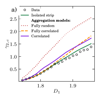
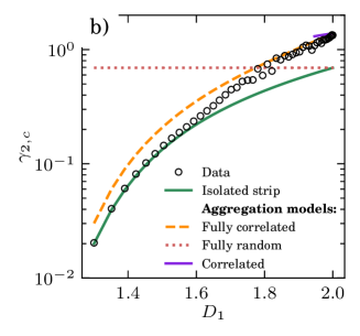
Figure 17: Decay exponent $\gamma_{2}$ of the variance of aggregated scalar levels with time, as a function of fractal dimension $D_{1}$ for a) sine flow and b) baker map. Dots stand for numerical simulations and lines from theoretical predictions for isolated lamellae (Eq. (96) and exponents of $\langle\rho^{-1}\rangle_{0}$ in Tables 1 and 2), fully correlated aggregation (Eq. (9) and exponents of $\langle\rho^{-2}\rangle_{0}$ in Tables 1 and 2), fully random aggregation (Eq. (7) and exponents of $1/\langle\rho\rangle_{0}$ in Tables 1 and 2) and correlated aggregation (Eq. (87)).

4.3 Effective aggregation number

The effect of correlated aggregation may be viewed as leading to an effective number of random aggregations, smaller than the actual number of aggregations. Assuming a random aggregation process, the distribution of concentrations (Fig. 15) would be fitted to a gamma distribution (Villermaux & Duplat, 2003a; Villermaux, 2019). The resulting shape parameter $k_{\text{eff}}$ may then be interpreted as an effective random aggregation number. From the variance of concentration (87), we have

$$k_{\text{eff}}=\frac{\mu_{c}^{2}}{\sigma^{2}_{c}}\sim\exp({\gamma_{2,c}\,t})=k^{\min(k_{n},\xi)},$$ (90)

where $k=\langle n\rangle$ is the actual mean number of aggregations of the material line. The effective mean number of independent and random aggregation events $k_{\text{eff}}$ is thus equal to the total number of aggregation events $k$ raised to the exponent $\min(k_{n},\xi)$. In general, for random flows, $\xi<1$ so that there is less independent aggregation than the mean. For instance, in random sine flows where the stretching heterogeneity may be tuned to reach fractal dimensions between 1.65 and 1.95 (Fig. 5), the correlation exponent varies between 0.45 and 0.6 (Fig. 14). Thus, the effective aggregation rate is about half of the total aggregation rate in random sine flows.

5 Conclusions

Scalar mixing in heterogeneous flows results from the interaction of fluid stretching, which creates elongated lamellar structures, and fluid compression, which leads to their aggregation and coalescence at the Batchelor scale. Classically, the aggregation process has been assumed to to obey fully random addition rules. In contrast, we show here that such process can be highly correlated, leading to the aggregation of lamellae of similar elongations. This correlated aggregation process significantly reduces the flow mixing efficiency compared to a random hypothesis, maintaining it close to the mixing efficiency for solitary lamellae and explaining the observed monotonic exponential decay of scalar variance before and after coalescence time Fereday et al. (2002).

Using two-dimensional chaotic flows as a reference, we measured the aggregation rate of exponentially stretched material lines across a broad range of chaotic flow regimes. We showed that the most elongated lamellae are also the most aggregated ones, due to the fact that larger compression rates attract a larger flow region. The link between elongation and compression, induced by incompressibility, hence generates a direct correlation between elongation and aggregation. The heterogeneity in stretching rates therefore controls the heterogeneity of the number of lamellae in bundles. We showed that the statistics of aggregated lamella numbers can be predicted from the fractal dimensions of the elongated material line. We then derived a general theoretical framework that captures the effect of correlated aggregation, where lamellae of similar stretching aggregate preferentially, and predict the pdfs of aggregated scalar levels. In this new framework, correlated aggregation is uniquely characterised by single correlation exponent $\xi$, which provides a measure of the effective number of random aggregation events. In that sense, correlated aggregation delays the route to uniformity compared to a fully random hypothesis, although it does not alter the fundamental nature of the aggregation process (Villermaux & Duplat, 2003a).

Our results apply for two-dimensional fully chaotic flows in the Batchelor regime, that is, for smooth velocity fields below the integral scale. These flow fields are representative of a large class of flows, including notably porous media flows (Heyman et al., 2020; Souzy et al., 2020). It is probable that different aggregation rules arise in rough flows or above the integral scale. Indeed, scalar mixing in rough turbulent flows has already been shown to be well captured by a fully random aggregation scenario (Duplat & Villermaux, 2008b). A remaining open question is thus to uncover the potential mechanisms leading to a loss of correlations from small diffusive scales to large dispersive scales. It should also be possible to extend the correlated aggregation theory to three-dimensional flows in the Batchelor regime. One-dimensional lamellar structures transform into thin two-dimensional sheets (Martínez-Ruiz et al., 2018) which also aggregate in the direction of their highest gradient (the direction of compression). A similar formalism should thus apply and could be the object of future work.

[Funding]Funded by the European Union (ERC, CHORUS, 101042466)

[Declaration of interests]The authors report no conflict of interest.

[Data availability statement]The data and codes to reproduce the findings of this study are openly available in Github at https://github.com/jorishey1234/aggregation

[Author ORCIDs]J. Heyman, https://orcid.org/0000-0002-0327-7924; T. Le Borgne, https://orcid.org/0000-0001-9266-9139; E. Villermaux, https://orcid.org/0000-0001-5130-4862; P. Davy, https://orcid.org/0000-0002-6648-0145

Appendix A Stretching statistics and averaging

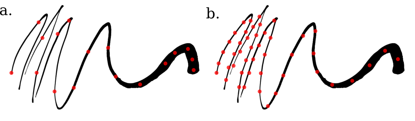
Figure 18: Different sampling procedures a. Uniformly over the initial filament b. uniformly over the final elongated filament

In random chaotic flows, varying stretching rates are experienced by fluid elements (Lester et al., 2013). Because of the multiplicative nature of stretching, the log-elongation of material elements $\log\rho$ is well approximated in ergodic chaotic flows by a sum of iid random variables, that converges towards the normal distribution with mean $\mu t$ and variance $\sigma^{2}t$ (Meunier & Villermaux, 2022)

$$P_{\rho,0}(\rho)\approx\frac{1}{\rho\sqrt{2\pi\sigma^{2}t}}\exp\left(-\frac{(\log\rho-\mu t)^{2}}{2\sigma^{2}t}\right)$$ (91)

Non-asymptotic stretching statistics can differ substantially from this limiting behavior. For instance, the baker map has a binomial distribution of elongations

$$P_{\rho,0}\left(\rho=(1-a)^{k}a^{t-k}\right)=\left(\begin{array}[]{c}t\\ k\end{array}\right)(1-a)^{k}a^{t-k},\text{ for }k=0\dots t,$$ (92)

which tends to a lognormal distribution with $\mu/t=-a\log(a)-(1-a)\log(1-a)$ and $\sigma^{2}/t=a(1-a)(\log(1-a)-\log(a))^{2}$.

Statistics of lamellar concentrations in the material line can then be obtained by suitable ensemble averaging (denoted by angle brackets) over this distribution. Depending on how sampling is performed through the material line (Fig. 18), different moments are obtained. Uniform sampling on the initial filament prior elongation, denoted $\langle\bullet\rangle_{0}$, leads to the distribution $P_{\rho,0}(\rho)$ (Eq. (91)) with main moments summarized in Table 1. In contrast, uniform sampling on a the final elongated material line of length $L$, denoted by $\langle\bullet\rangle_{L}$ leads to the weighted pdf $P_{\rho,{L}}\sim\rho P_{\rho,{0}}$. $P_{\rho,{L}}$ is thus also lognormal, but with different mean, $(\mu+\sigma^{2})t$. Uniform sampling on the final material line (Fig.18a) gives a stronger weights to highly elongated part of the material line than uniform sampling on the initial filaments (Fig.18b). Moments of $\log\rho$, $\rho$ and $\rho^{-1}$ are summarized in Tables 1 for sine flow and 2 for the baker map for initial and final sampling. Note that we impose $\rho\geq 1$ since the one-dimensional lamellar framework is valid only when lamellae elongates in the $y$ direction. This lower bound creates a particular scaling of moments of $\rho^{-1}$ when $\sigma^{2}$ is larger than $\mu$, that is when weak stretching rates dominate the ensemble average.

	$\log\rho$	$\rho$	$\rho^{-1}$
$\langle\bullet\rangle_{0}$	$\mu t$	$e^{(\mu+\sigma^{2}/2)t}$	$\left\{\begin{matrix}e^{-(\mu-\sigma^{2}/2)t}&\text{ if }\mu\geq\sigma^{2}\\ e^{-\mu^{2}/(2\sigma^{2})t}&\text{ if }\mu\leq\sigma^{2}\end{matrix}\right.$
$\langle\bullet^{2}\rangle_{0}$	$\sigma^{2}t$	$e^{(2\mu+2\sigma^{2})t}$	$\left\{\begin{matrix}e^{-2(\mu-\sigma^{2})t}&\text{ if }\mu\geq 2\sigma^{2}\\ e^{-\mu^{2}/(2\sigma^{2})t}&\text{ if }\mu\leq 2\sigma^{2}\end{matrix}\right.$
$\langle\bullet\rangle_{L}$	$(\mu+\sigma^{2})t$	$e^{(\mu+3\sigma^{2}/2)t}$	$e^{(-\mu-\sigma^{2}/2)t}$
$\langle\bullet^{2}\rangle_{L}$	$\sigma^{2}t$	$e^{(2\mu+4\sigma^{2})t}$	$\left\{\begin{matrix}e^{-2\mu t}&\text{ if }\mu\geq\sigma^{2}\\ e^{-(\mu+\sigma^{2})^{2}/(2\sigma^{2})t}&\text{ if }\mu\leq\sigma^{2}\end{matrix}\right.$

Table 1: Moments of log-normally distributed stretching sampled over infinitesimal fluid elements ($\langle\bullet\rangle_{0}$), material line ($\langle\bullet\rangle_{L}$) .

	$\log\rho$	$\rho$	$\rho^{-1}$
$\langle\bullet\rangle_{0}$	$(-a\log(a)-(1-a)\log(1-a))t$	$2^{t}$	$(1-2a+2a^{2})^{t}$
$\langle\bullet^{2}\rangle_{0}$	$a(1-a)(\log(1-a)-\log(a))^{2}t$	$-$	$(1-3a+3a^{2})^{t}$

Table 2: Moments of binomial distributed stretching sampled over infinitesimal fluid elements ($\langle\bullet\rangle_{0}$), material line ($\langle\bullet\rangle_{L}$).

Appendix B Decay of scalar variance

A key challenge in modeling mixing is to capture the decay of the scalar variance $\sigma^{2}_{c}$. The spatial variance of a solitary strip on a domain with surface $\mathcal{A}$ can be obtained by the integration of $\Theta^{2}(x,t)$ (Eq. 36 of the manuscript) in the transverse direction $x$, averaged over the elongation of the filament. This yields

$$\langle c^{2}\rangle = \mathcal{A}^{-1}\left\langle\ell_{0}\rho\int_{-\infty}^{+\infty}\Theta(x,t)^{2}\text{d}x\right\rangle_{0}$$ (93)

$$= \mathcal{A}^{-1}\sqrt{\frac{\pi}{2}}\ell_{0}\langle\rho s\theta^{2}\rangle_{0}$$ (94)

$$= \mathcal{A}^{-1}\sqrt{\frac{\pi}{2}}s_{0}\ell_{0}\theta_{0}\langle\theta\rangle_{0},$$ (95)

where the averaging was defined in Section A. At large time, using Eq. (42) of the manuscript,

$$\langle c^{2}\rangle \to \frac{\theta_{0}^{2}\ell_{0}s_{0}}{\mathcal{A}}\sqrt{\frac{\pi}{2}}\sqrt{Pe_{0}}\langle\rho^{-1}\rangle_{0}.$$ (96)

Typical asymptotic scaling of $\langle\rho^{-1}\rangle_{0}$ in the baker map and the sine flow are reported in Table. 1.

Appendix C Statistics among bundles of similar size

The variability of a set of random numbers is always greater than the average variability of a subset of these numbers. Thus, the stretching variance among bundles of similar sizes– denoted $\sigma^{2}_{\rho^{-1},n}$– is always larger than the average stretching variance inside the bundle (Eq. (74)). We have

$$\sigma^{2}_{\rho^{-1},n}=\left(\frac{n}{n-1}\right)\sigma^{2}_{\rho^{-1}|n}.$$ (97)

For instance, for bundles made of two lamellae, we expect $\sigma^{2}_{\rho^{-1},n}$ to be twice larger as $\sigma^{2}_{\rho^{-1}|n}$ given by Eq. (74). The difference between the statistics of the set and its subset tends to reduce at large $n$, where $\sigma^{2}_{\rho^{-1}|n}\to\sigma^{2}_{\rho^{-1},n}$. For $n=1$, both $\sigma^{2}_{\rho^{-1}|n}$ and $n-1$ cancel out, so that the previous equation is undetermined.

Assuming that bundles of similar size have independent stretching histories, the variability of the aggregated scalar concentration is obtained from independent realisations of the random sum (Eq. (47)). Thus, the variance of $c|n$ reads

$$\sigma^{2}_{c|n}=n\left(\frac{\sqrt{\pi}\theta_{0}s_{0}}{s_{B}}\right)^{2}\sigma^{2}_{\rho^{-1},n}=\left(\frac{\sqrt{\pi}\theta_{0}s_{0}}{s_{B}}\right)^{2}\sigma^{2}_{\rho^{-1}|n}\left(\frac{n^{2}}{n-1}\right)=\frac{(\sqrt{\pi}\theta_{0}\ell_{0}s_{0})^{2}}{\mathcal{A}^{2}}\left(\frac{n^{2-\tilde{\gamma}}-1}{n-1}\right).$$ (98)

When $n$ is large, however, we recover

$$\sigma^{2}_{c|n}\sim n^{-\tilde{\gamma}+1},$$ (99)

References

- Batchelor (1959) Batchelor, G. K. 1959 Small-scale variation of convected quantities like temperature in turbulent fluid part 1. general discussion and the case of small conductivity. J. Fluid Mech. 5 (1), 113–133.
- Duplat et al. (2010) Duplat, J., Jouary, A. & Villermaux, E. 2010 Entanglement rules for random mixtures. Phys. Rev. Lett. 105, 034504.
- Duplat & Villermaux (2008a) Duplat, Jerôme & Villermaux, Emmanuel 2008a Mixing by random stirring in confined mixtures. Journal of Fluid Mechanics 617, 51–86.
- Duplat & Villermaux (2008b) Duplat, J. & Villermaux, E. 2008b Mixing by random stirring in confined mixtures. J. Fluid Mech. 617, 51–86.
- Farmer et al. (1983) Farmer, J Doyne, Ott, Edward & Yorke, James A 1983 The dimension of chaotic attractors. Physica D: Nonlinear Phenomena 7 (1-3), 153–180.
- Fereday et al. (2002) Fereday, DR, Haynes, PH, Wonhas, A & Vassilicos, JC 2002 Scalar variance decay in chaotic advection and batchelor-regime turbulence. Physical Review E 65 (3), 035301.
- Finn & Ott (1988) Finn, John M & Ott, Edward 1988 Chaotic flows and fast magnetic dynamos. The Physics of fluids 31 (10), 2992–3011.
- Giona et al. (2001) Giona, M, Cerbelli, S & Adrover, A 2001 Geometry of reaction interfaces in chaotic flows. Physical review letters 88 (2), 024501.
- Grassberger (1983) Grassberger, Peter 1983 Generalized dimensions of strange attractors. Physics Letters A 97 (6), 227–230.
- Haynes & Vanneste (2005) Haynes, Peter H & Vanneste, Jacques 2005 What controls the decay of passive scalars in smooth flows? Physics of Fluids 17 (9), 097103.
- Heyman et al. (2021) Heyman, J., Lester, D. R. & Le Borgne, T. 2021 Scalar signatures of chaotic mixing in porous media. Phys. Rev. Lett. 126, 034505.
- Heyman et al. (2020) Heyman, Joris, Lester, Daniel R., Turuban, Régis, Méheust, Yves & Le Borgne, Tanguy 2020 Stretching and folding sustain microscale chemical gradients in porous media. Proceedings of the National Academy of Sciences 117 (24), 13359–13365.
- Le Borgne et al. (2013) Le Borgne, T., Dentz, M. & Villermaux, E. 2013 Stretching, coalescence and mixing in porous media. Phys. Rev. Lett. 110, 204501.
- Le Borgne et al. (2015) Le Borgne, T., Dentz, M. & Villermaux, E. 2015 The lamellar description of mixing in porous media. J. Fluid Mech. 770, 458–498.
- Le Borgne et al. (2017) Le Borgne, T., Huck, P. D., Dentz, M. & Villermaux, E. 2017 Scalar gradients in stirred mixtures and the deconstruction of random fields. J. Fluid Mech. 812, 578–610.
- Lester et al. (2016) Lester, D. R., Dentz, M. & Le Borgne, T. 2016 Chaotic mixing in three-dimensional porous media. J. Fluid Mech. 803, 144–174.
- Lester et al. (2013) Lester, D. R., Metcalfe, G. & Trefry, M. G. 2013 Is chaotic advection inherent to porous media flow? Phys. Rev. Lett. 111, 174101.
- Martínez-Ruiz et al. (2018) Martínez-Ruiz, Daniel, Meunier, Patrice, Favier, Benjamin, Duchemin, Laurent & Villermaux, Emmanuel 2018 The diffusive sheet method for scalar mixing. Journal of Fluid Mechanics 837, 230–257.
- Meunier & Villermaux (2010) Meunier, P. & Villermaux, E. 2010 The diffusive strip method for scalar mixing in two dimensions. J. Fluid Mech. 662, 134–172.
- Meunier & Villermaux (2022) Meunier, Patrice & Villermaux, Emmanuel 2022 The diffuselet concept for scalar mixing. Journal of Fluid Mechanics 951, A33.
- Ott & Antonsen Jr (1989) Ott, Edward & Antonsen Jr, Thomas M 1989 Fractal measures of passively convected vector fields and scalar gradients in chaotic fluid flows. Physical Review A 39 (7), 3660.
- Ottino (1990) Ottino, J.M. 1990 Mixing, chaotic advection, and turbulence. Annu. Rev. Fluid Mech. 22, 207–253.
- Ranz (1979) Ranz, William E. 1979 Applications of a stretch model to mixing, diffusion, and reaction in laminar and turbulent flows. AIChE J. 25 (1), 41–47.
- Schwartz & Yeh (1982) Schwartz, Stuart C & Yeh, Yu-Shuan 1982 On the distribution function and moments of power sums with log-normal components. Bell System Technical Journal 61 (7), 1441–1462.
- Souzy et al. (2020) Souzy, M., Lhuissier, H., Méheust, Y., Le Borgne, T. & Metzger, B. 2020 Velocity distributions, dispersion and stretching in three-dimensional porous media. Journal of Fluid Mechanics 891, A16.
- Tang & Boozer (1996) Tang, Xian Zhu & Boozer, Allen H 1996 Finite time lyapunov exponent and advection-diffusion equation. Physica D: Nonlinear Phenomena 95 (3-4), 283–305.
- Tsang et al. (2005) Tsang, Yue-Kin, Antonsen Jr, Thomas M & Ott, Edward 2005 Exponential decay of chaotically advected passive scalars in the zero diffusivity limit. Physical Review E 71 (6), 066301.
- Villermaux (2012) Villermaux, Emmanuel 2012 On dissipation in stirred mixtures. Advances in applied mechanics 45, 91–107.
- Villermaux (2019) Villermaux, Emmanuel 2019 Mixing versus stirring. Annu. Rev. Fluid Mech. 51 (1), 245–273.
- Villermaux & Duplat (2003a) Villermaux, Emmanuel & Duplat, Jérôme 2003a Mixing as an aggregation process. Physical review letters 91 (18), 184501.
- Villermaux & Duplat (2003b) Villermaux, E. & Duplat, J. 2003b Mixing as an aggregation process. Phys. Rev. Lett. 91 (18), 184501–1–4.
- Villermaux & Duplat (2006) Villermaux, Emmanuel & Duplat, Jérôme 2006 Coarse grained scale of turbulent mixtures. Physical review letters 97 (14), 144506.
- Wonhas & Vassilicos (2002) Wonhas, A & Vassilicos, JC 2002 Mixing in fully chaotic flows. Physical Review E 66 (5), 051205.