Applicability and limitations of cluster perturbation theory for Hubbard models
Abstract
We present important use cases and limitations when considering results obtained from Cluster Perturbation Theory (CPT). CPT combines the solutions of small individual clusters of an infinite lattice system with the Bloch theory of conventional band theory in order to provide an approximation for the Green’s function in the thermodynamic limit. To this end we are investigating single-band and multi-band Hubbard models in one- and two-dimensional systems. A special interest is taken in the supposed pseudo gap regime of the two-dimensional square lattice at half filling and intermediate interaction strength () as well as the metal-insulator transition. We point out that the finite-size level spacing of the cluster limits the resolution of spectral features within CPT. This restricts the investigation of asymptotic properties of the metal-insulator transition, as it would require much larger cluster sizes that are beyond computational capabilities.
I Introduction
The Hubbard model probably belongs to the most studied systems in solid state theory. Although its Hamiltonian possesses a simple form, it captures important aspects of various many-body phenomena like Mott-insulating states, antiferromagnetism and superconductivity.reich_heavy-fermion_1988 ; tremblay_pseudogap_2006 ; huscroft_pseudogaps_2001 ; gull_superconductivity_2013 ; Arovas_hubbard_model . The Hamiltonian has three terms: the first term describes the hopping of the electrons on the lattice, the second term a repulsive Coulomb interaction of spin up and spin down electrons on the same site and the third term is the chemical potential, which we shifted such that half filling corresponds to for bi-partite lattices:
| (1) |
where and are labelling the lattice sites and denotes the spin index. With we denote the fermionic creation and annihilation operators and is the occupation number operator.
One interesting aspect of the Hubbard model is its Mott-insulating state at high interaction strength as well as the associated metal-insulator transition it supposedly captures. In this regard a pseudogap regime at intermediate interaction strength has been discussed tremblay_pseudogap_2006 ; schafer_fate_2015 . Within this study we investigated this regime using Cluster Perturbation Theory (CPT). Introduced by Senechal et al. senechal_spectral_2000 CPT has shown remarkable results when applied to the Hubbard model, despite being of low numerical cost. While these results caught our initial interest for the method, we came to the conclusion that care has to be taken when interpreting the results of CPT, especially concerning features like spectral gaps. In the following, we will first outline the method, apply it to the systems of interest and then analyse carefully the accuracy of the results by comparing the one dimensional case to exact results using Bethe ansatz.
II Methods
II.1 Cluster Green’s functions
In Cluster Perturbation Theory (CPT) the main objective is to construct an approximation to the retarded Green’s function of a given lattice system in the thermodynamic limit. This function is especially useful as it provides direct access to the spectral function bruus_many-body_2004 ; fetter2012quantum :
| (2) |
As CPT aims at approximating the Green’s function of the full system by combining the solutions of small finite clusters cut out of the infinite lattice, we first have to discuss how to obtain the interacting Green’s function on such a cluster. For this we first define the retarded Green’s function for two fermionic operators and as:
| (3) |
where is the anticommutator, and are time arguments and is the Heavyside Theta function. Note that we are only interested in the case, which means that the expectation value () only consists of the ground state . For the retarded Green’s function we have and as the Hamiltonian of interest is time-independent, we can assume to be zero. As we are going to use a Chebyshev expansion, it is convenient to rewrite the retarded Green’s function in terms of two new functions and schmitteckert_calculating_2010 :
| (4) |
Where we used the definitions:
| (5) | ||||
| (6) |
Performing a Fourier transformation we can obtain the Green’s function in the frequency domain as:
| (7) |
| (8) |
where is an infinitesimal parameter that ensures convergence.
II.2 Chebyshev Expansion
Expressions like (7) and (8) can be very efficiently handled using Chebyshev polynomials braun_numerical_2014 . They contain the function
| (9) |
with and , that can be expanded using Chebyshev polynomials of the first kind :
| (10) |
with the expansion coefficients:
| (11) |
For the polynomials the following recursion relation holds:
| (12) |
| (13) |
| (14) |
where we choose the two parameters to fit the spectrum of the operator into the interval , required by the orthogonality relation of the Chebyshev polynomials. With this we can identify the Green’s functions as:
| (15) |
where the are often referred to as Chebyshev moments and are defined as the expectation values of the polynomials:
| (16) |
In order to calculate these moments for the Green’s function of the finite cluster, we require the Hamiltonian in a many particle basis. To construct the ground state we employ a sparse matrix diagonalization as for example introduced in Ref. senechal_introduction_2010 . The main idea is to explicitly encode how a specific Hamiltonian acts on basis states in the occupation number representation. For this, one needs to at least encode all the basis states in a particular number sector. Although this can be efficiently done by saving each basis state as the bitwise representation of an integer, the computational space still grows exponentially, making it only usable for very small clusters. Due to limited computational resources our calculations did not exceed 18 site calculations. Having constructed the Hamiltonian the groundstate can be calculated using a Lanczos algorithm.
II.3 Cluster Perturbation Theory
The goal of Cluster Perturbation Theory (CPT) is to approximate the Green’s function of a particular lattice model in the thermodynamic limit by combining the Green’s functions of small individual clusters, for example calculated as described in the previous section. Introductions to this method are presented in Ref. senechal_introduction_2010 ; pavarini_ldadmft_2011 . The first step is to split the Hamiltonian into two parts:
| (17) |
In the first part:
| (18) |
one has the full Hubbard model on small, individual clusters , each labeled by the index and in the second part:
| (19) |
we only have the hopping elements between these individual clusters. Note that due to this splitting, it can be very useful to describe any lattice site by a combination of two new vectors:
| (20) |
where is the position of the individual clusters in
a new superlattice and describes the position
of an individual site within a cluster.
One can calculate the Green’s function for one of these clusters
and use this result for the Green’s function of all other clusters due
to the lattice symmetry. We will refer to this Green’s function as the cluster
Green’s function . The main
idea within CPT consists in calculating the self-energy from the cluster Green’s
function and use it to construct an approximation for the self-energy
of the full system. We can obtain the cluster self-energy
from a Dyson equation:
| (21) |
where is the non-interacting Green’s function on the cluster defined as:
| (22) |
Therefore we obtain for a particular entry of the system self-energy in real space, connecting two sites on the same cluster:
| (23) |
and all entries of the self-energy connecting sites on different
clusters are set to zero.
Finally, we can use this approximation of the self energy,
namely using the cluster self energy for the self energy of the full system,
in a Dyson equation as before, to obtain the
Green’s function of the full system:
| (24) |
Note that in this way, we treat the non-interacting part exactly. This is why one should view the CPT approximation as a perturbation theory in rather than a perturbation in the inter-cluster hopping. Finally we end up with the following expression for the Green’s function of the full system:
| (25) |
II.4 Periodization
While the just described procedure works for finite systems, it is important to note that there are also so called periodization schemes, which allow to extend these results to infinite systems. Here we are going to use the so called G-scheme, as discussed in Ref. avella_strongly_2012 . The main idea is based on arranging clusters in an infinite superlattice and exploiting its translational symmetry. As pointed out before, one can split any lattice vector into one vector defined on the superlattice and one on a cluster. Therefore, one can similarly split any wave vector k of the 1st BZ into a combination of a wave vector in a reduced BZ associated with the superlattice and one of the Brillouin zone of a single cluster K. This also allows one to split the Fourier transformations into two parts, one for the cluster and one for the superlattice. Using Bloch’s theorem for the superlattice, one ends up with the following form for a periodized Green’s function:
| (26) |
III Results
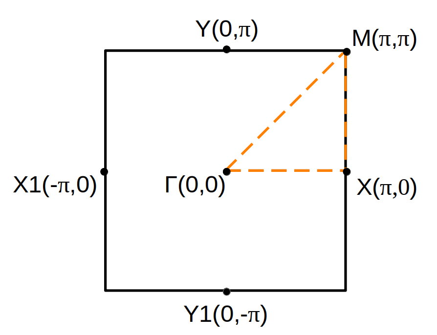
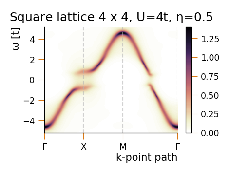
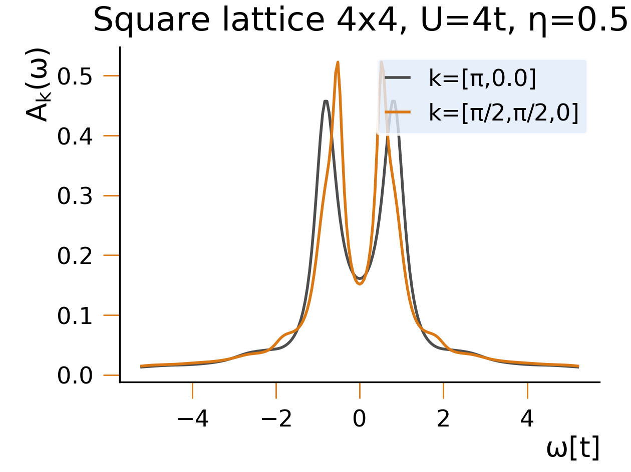
We can now use the just presented methods to calculate the spectral function for our main system of interest, the 2D Hubbard model on a square lattice at half filling (Fig. 1, 2, 3). As we can clearly see when considering the spectral function at the point and in the midpoint between and , CPT here suggests a considerable spectral weight in the gap at U=4t. However, we are going to show that there are two parameters that pose large additional constraints on the resolution that can actually be achieved using CPT. The first parameter is the convergence aiding factor and the second is the finite cluster size. While the artefacts induced by the convergence aiding factor are related to our approximation of using only a finite number of Chebyshev moments, the constraints imposed by the finite cluster size are an inherent limitation of CPT. These additional constraints are typically not discussed in detail in the literature, but as we are going to show they actually prohibit us from making accurate judgements about the pseudogap at intermediate interaction strengths. To see this, we will concentrate on the 1D Hubbard model since on the one hand it allows us to compare to exact results from Bethe ansatz and on the other hand it gives a higher resolution in k-space.
III.1 Convergence Aiding Factor
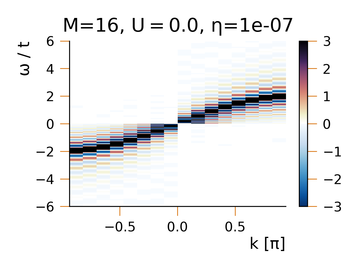
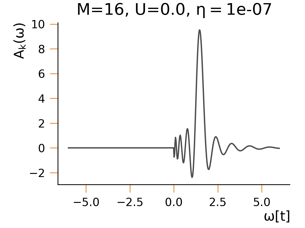
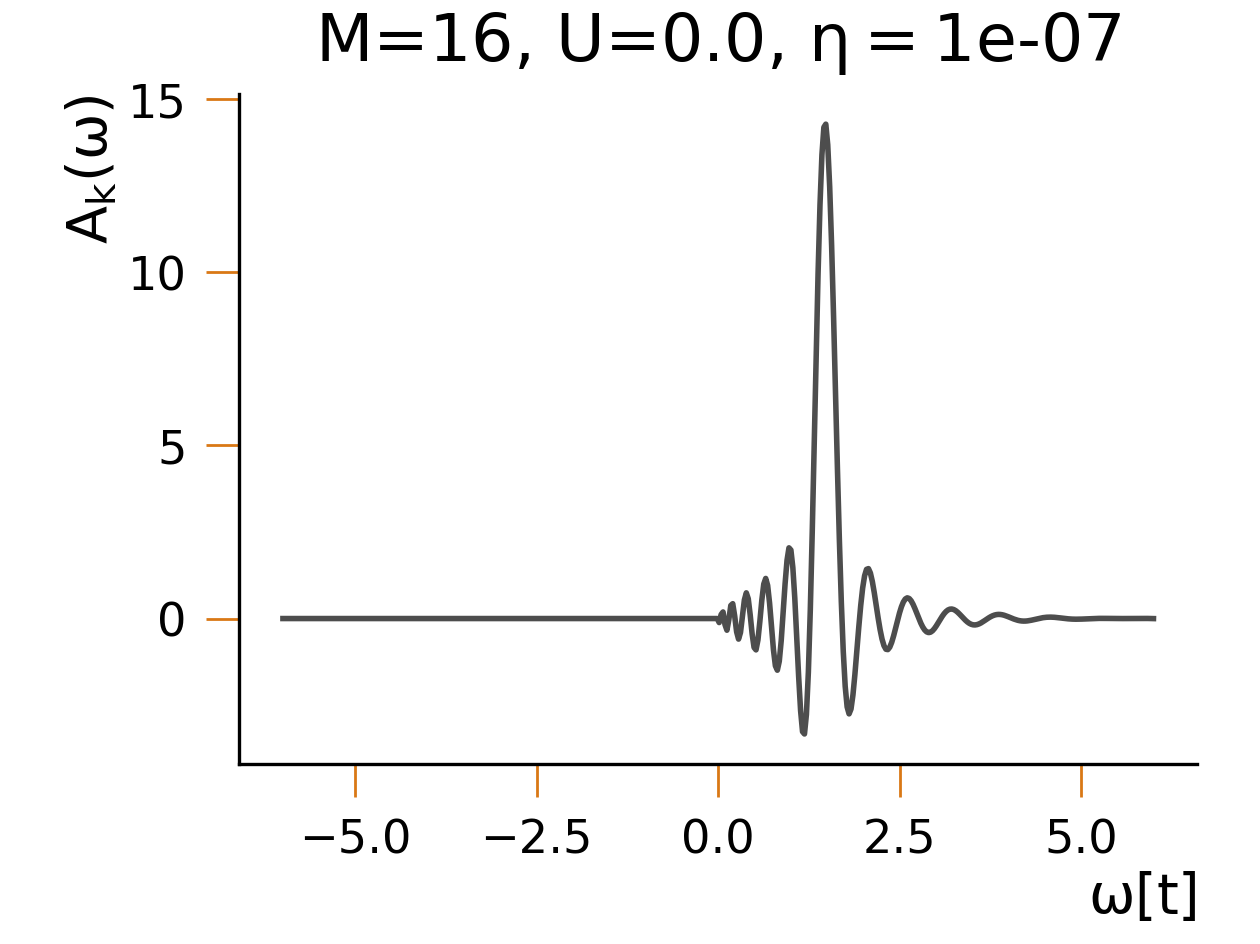
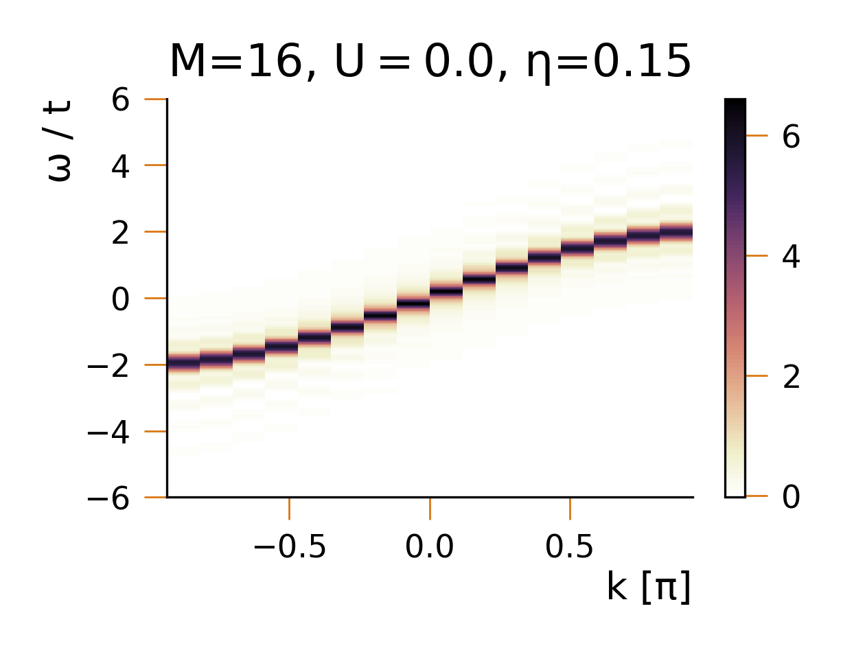
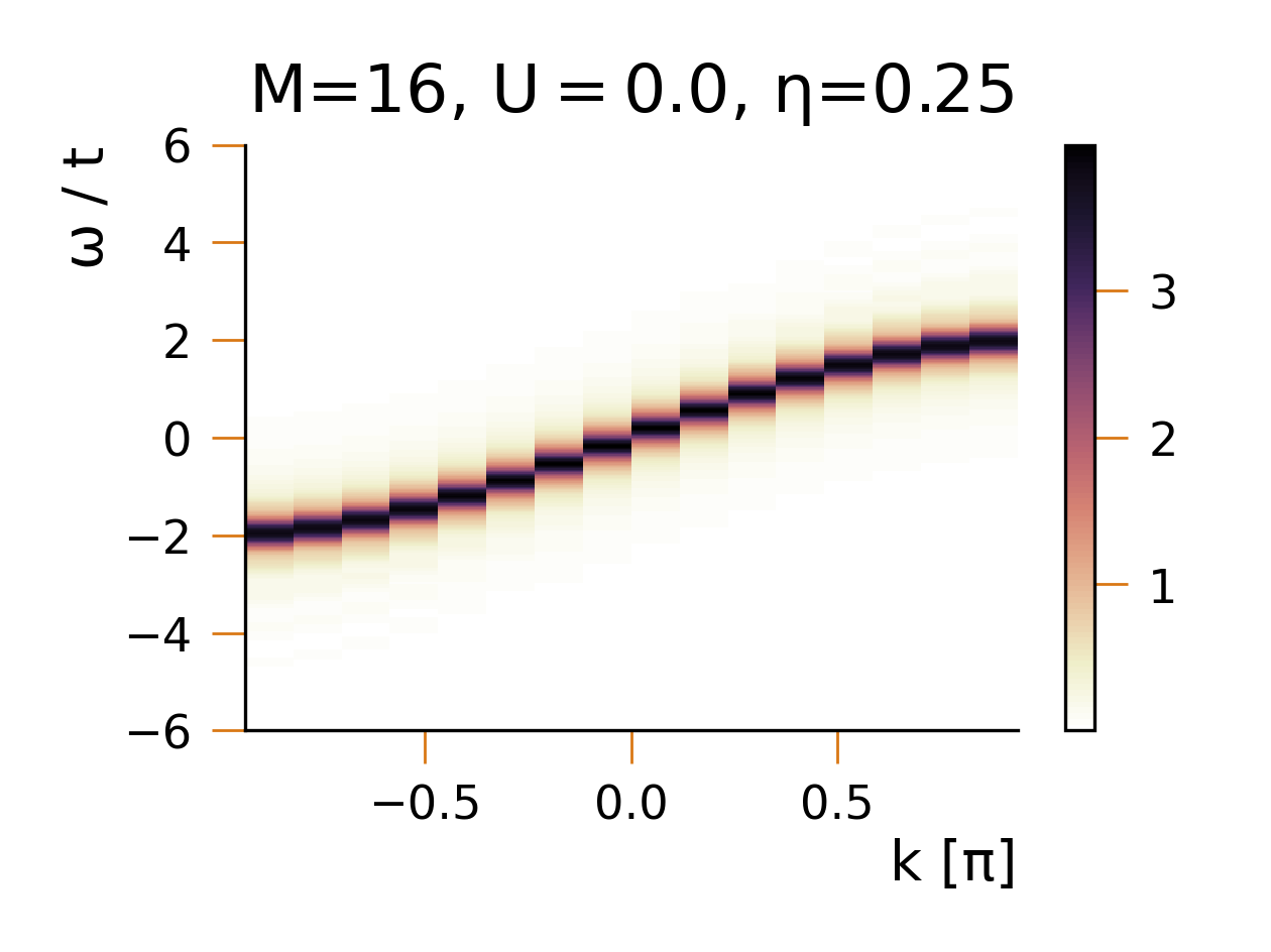
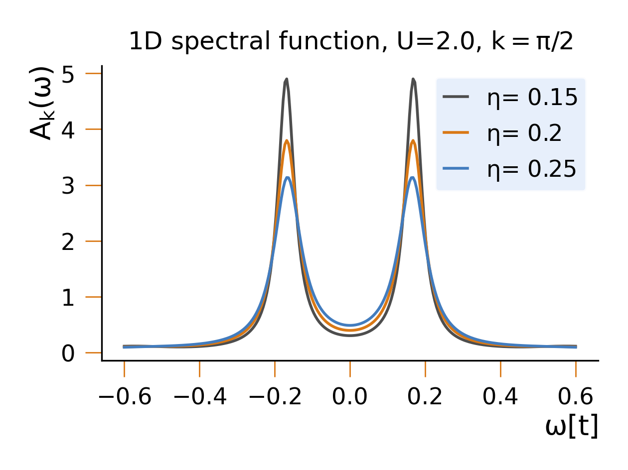
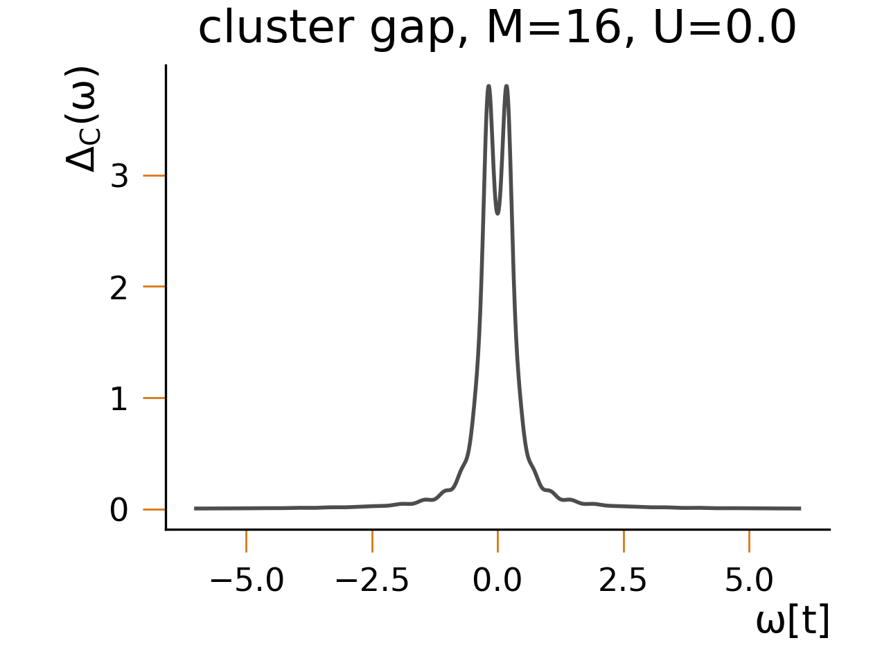
The convergence aiding factor enters the Green’s function in Eqs. (7) and (8). We calculate these Green’s functions with the help of the Chebyshev expansion (15) that, in practise, is evaluated only with a finite number of Chebyshev moments. This leads to artefacts in the spectral function in the form of Gibbs oscillations. This is illustrated for the spectral function of the non-interaction 1D chain evaluated for a cluster with 16 sites, see Fig. 4. In Fig. 5 we show the spectral function for a specific k-value as a function of frequency that clearly displays oscillations. Note that a higher Chebyshev order only increases the frequency of these oscillations (see Fig. 6) but does not change their magnitude. These oscillations can be identified as Gibbs oscillations that usually arise when approximating a sharp step function (in this case the -peak) by a finite Fourier expansion series. In order to suppress these artificial oscillations we will choose a sufficiently large value for the broadening parameter , such that the Chebyshev expansion is capable of resolving the peak without Gibbs oscillations. In addition, the finite cluster is naturally characterized by a finite level spacing. In order to mimic an infinite system and to obtain smooth bands, a finite broadening parameter has to be chosen such that it smears out the effect of the finite level spacing schmitteckert_calculating_2010 .
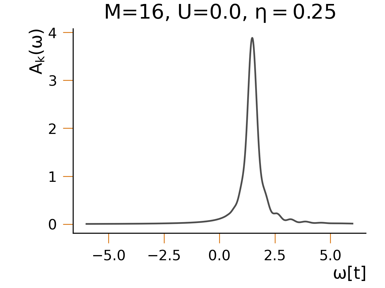
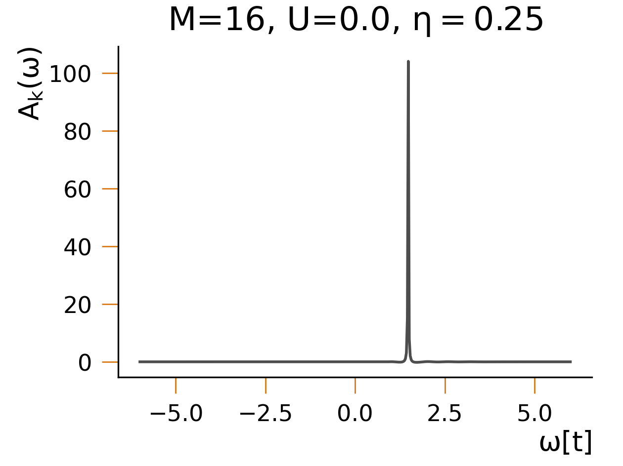
While this means that altogether one has to choose rather large (Fig. 7), one should also realize that one can counteract the effects of this broadening to a large extend by including the same large parameter for in the non interacting Green’s function when calculating the self energy. Effectively this corresponds to subtracting from the inverse of the Green’s function,
| (27) |
While this procedure works extremely well, as shown in Fig. 8, it still depends on the exact choice for , and it is a priori unclear which value to choose for . Here we want to propose two different approaches.
The first approach uses the typical single particle level spacing of the non interacting cluster for the broadening parameter , that can be estimated as
| (28) |
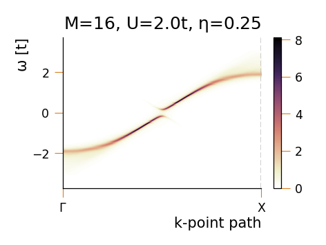
where is the bandwidth with the hopping amplitude and the cluster size. This smears the discrete cluster levels (Fig. 9), and leads to a good approximation of the continuous cosine band structure one expects for a 1D system (Fig. 10). Applying this choice for the CPT approximation to the 1D Hubbard model, one finds a finite spectral weight within the Hubbard gap illustrating the numerical artefact that is induced by a large , see Figs. 11 and 12.
As a second approach we propose an extrapolation scheme that calculates the CPT Green’s function for multiple values of and performs an extrapolation of the results to (see Figs. 13 and 14).
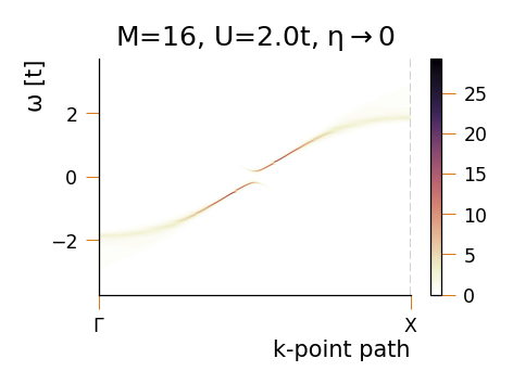
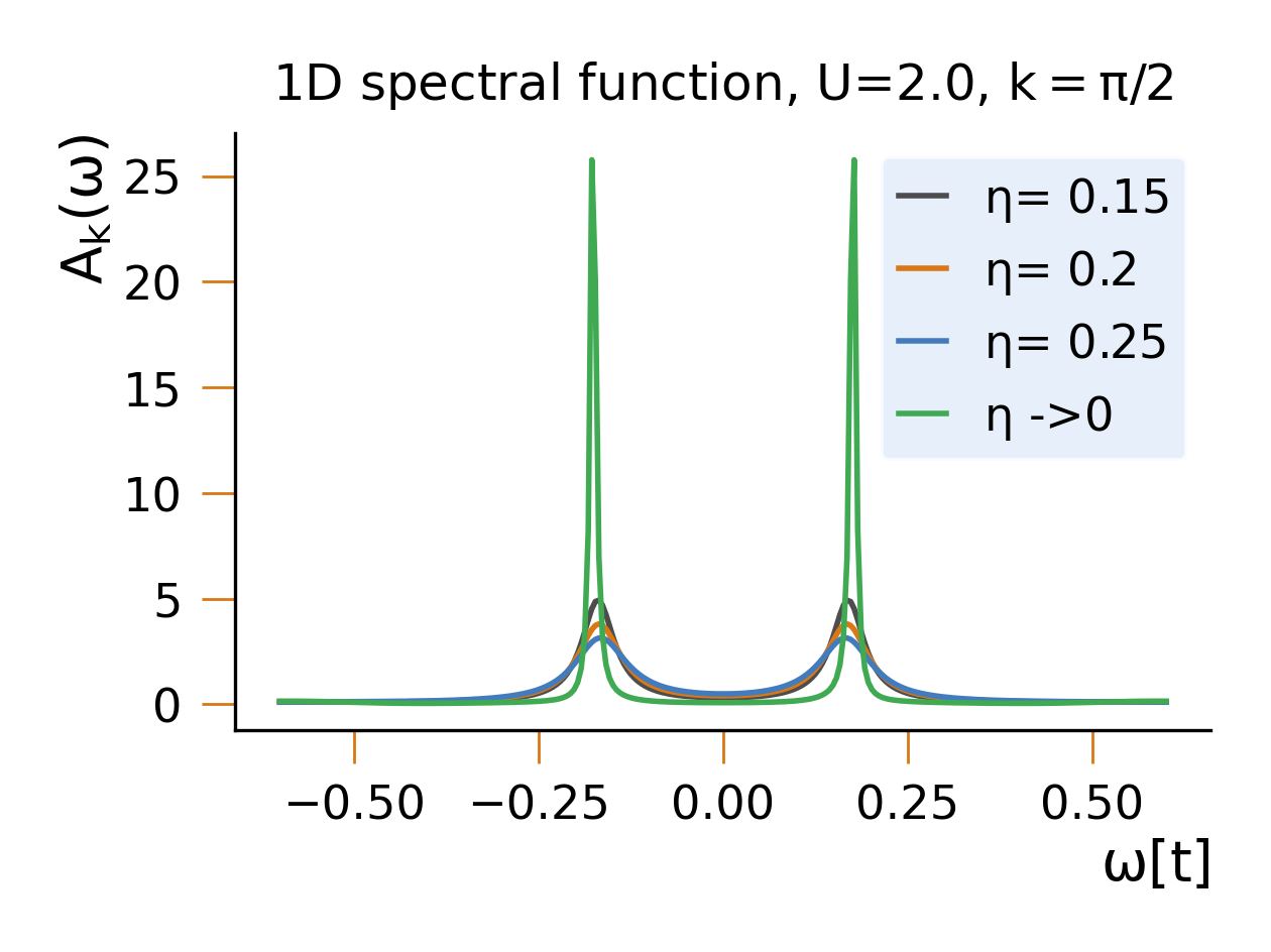
Although this procedure is physically sound and results in sharp peaks, there is no guarantee that this procedure will lead to the correct thermodynamic limit. In addition, obtaining a sharper peak does not automatically provide a more accurate result. Only in cases where the actual width of the peak is resolved by the Chebyshev expansion, i.e. wider than the many particle bandwidth divided by the number of Chebyshev moments, the extrapolated peaks could be considered reliable. Remarkably, despite the peak height and width being dependent, the peak position appears to be rather stable against a variation of .
III.2 Accuracy of CPT results
It is important to note that the finite size level spacing of the cluster used within CPT acts as a cutoff that limits any spectral resolution. Spectral features like gaps can only be resolved reliably if they are larger than this cutoff. As far as interaction effects are concerned, CPT only accurately reflects the same information that a careful analysis of the cluster result would also provide.
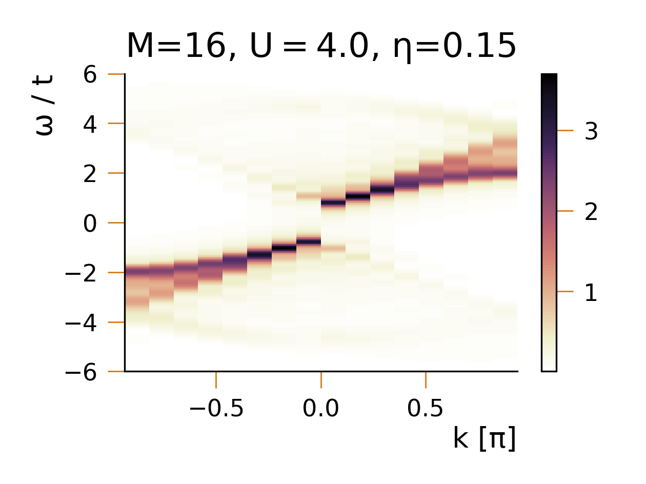
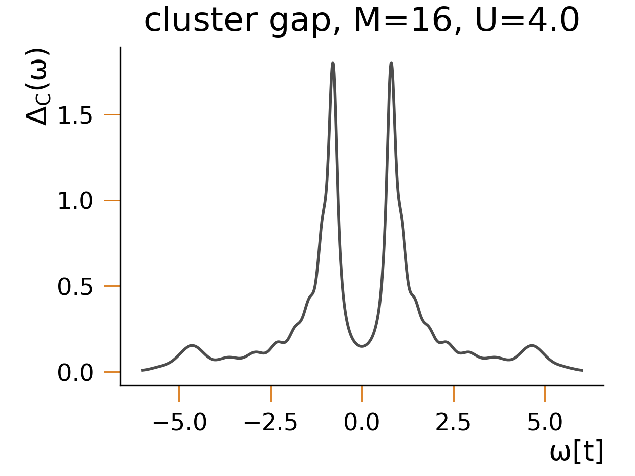
To extract such an information from the cluster result directly, let us consider the spectral function of a 16 site 1D Hubbard chain without interaction as was shown in Fig. 9 and with an interaction of U=4t (Fig. 15). As one would expect for the non interacting case we can see 16 individual levels forming a cosine shaped band, while for the interacting case the levels in the middle of the spectrum move apart. Hence, the actual band gap is given by the shift of the energy levels rather than their frequency difference directly. Table 1 shows the frequency difference of a particular interaction strength subtracted by the difference in the non interacting case, while the table below shows the exact results one would get in the thermodynamic limit using Bethe ansatz (Tab. 2). As we can see, only for the gap size agrees up to the second decimal place with the exact result. However, this means that for and using CPT with the currently computationally accessible cluster sizes we can not judge if there is an actual gap in the system, as the deviation is on the same order of magnitude as the actual gap. Additionally we can see that the gap size does not change significantly with the cluster size. Hence we have to assume that the considered cluster sizes are simply to small to resolve the gap accurately.
| M | U=1t | U=2t | U=4t | U=8t | |
|---|---|---|---|---|---|
| 6 | 0.03 | 0.16 | 0.66 | 2.24 | |
| 8 | 0.03 | 0.15 | 0.64 | 2.24 | |
| 10 | 0.02 | 0.14 | 0.63 | 2.24 | |
| 12 | 0.02 | 0.13 | 0.62 | 2.25 | |
| 14 | 0.02 | 0.13 | 0.62 | 2.26 | |
| 16 | 0.03 | 0.13 | 0.63 | 2.30 |
Now in order to arrive at the same result using the full CPT calculation, we can simply plot the spectral function in the middle of the spectrum. If we do this for multiple cluster sizes (Fig. 18), we can see, that the peaks slightly move to the center with increasing cluster size. Hence we can extrapolate the peak positions for the gap of an infinite cluster as shown in Fig. 19. This results in gaps comparable to results obtained directly from the cluster (Tab. 1). As in the case where we just considered the cluster we see that the error is too large to judge the gap accurately at .

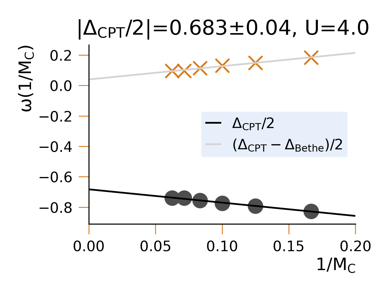
| U=1t | U=2t | U=4t | U=8t | |
| 0.003 | 0.086 | 0.643 | 2.340 | |
| 0.028 | 0.143 | 0.683 | 2.344 | |
| 0.025 | 0.057 | 0.040 | 0.004 |
After this discussion, we now return to the 2D case which sparked this investigation in the first place. We come to the conclusion that CPT is not able to resolve reliably the spectral weight within the gap and, in particular, to predict the presence or absence of a pseudogap despite the resolution that the plot in Fig. 2 suggests. This is, firstly, due to the influence of the finite broadening parameter used to dampen the Gibbs oscillation induced by the Chebyshev approximation, and, secondly, due to the finite level spacing associated with the chosen 2D cluster.
III.3 Use Cases for CPT
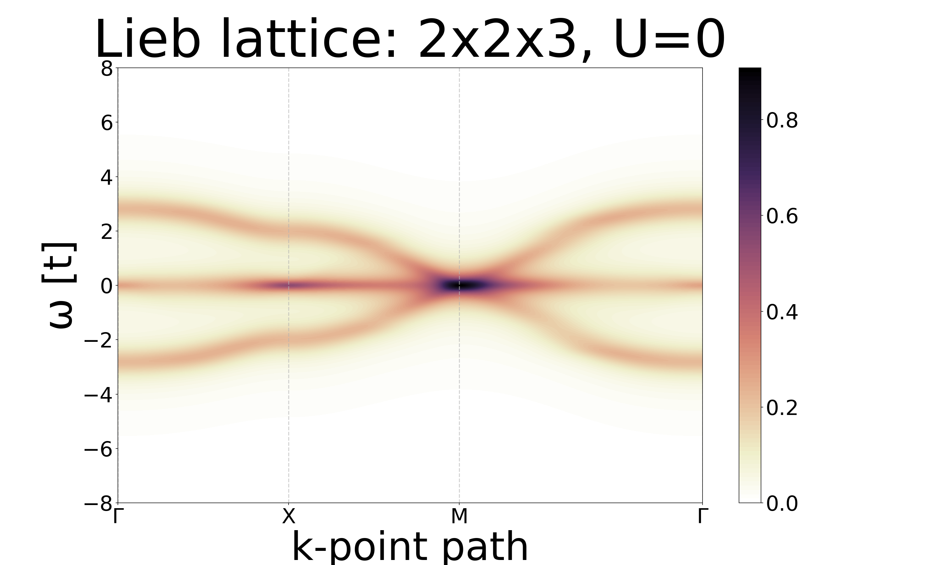
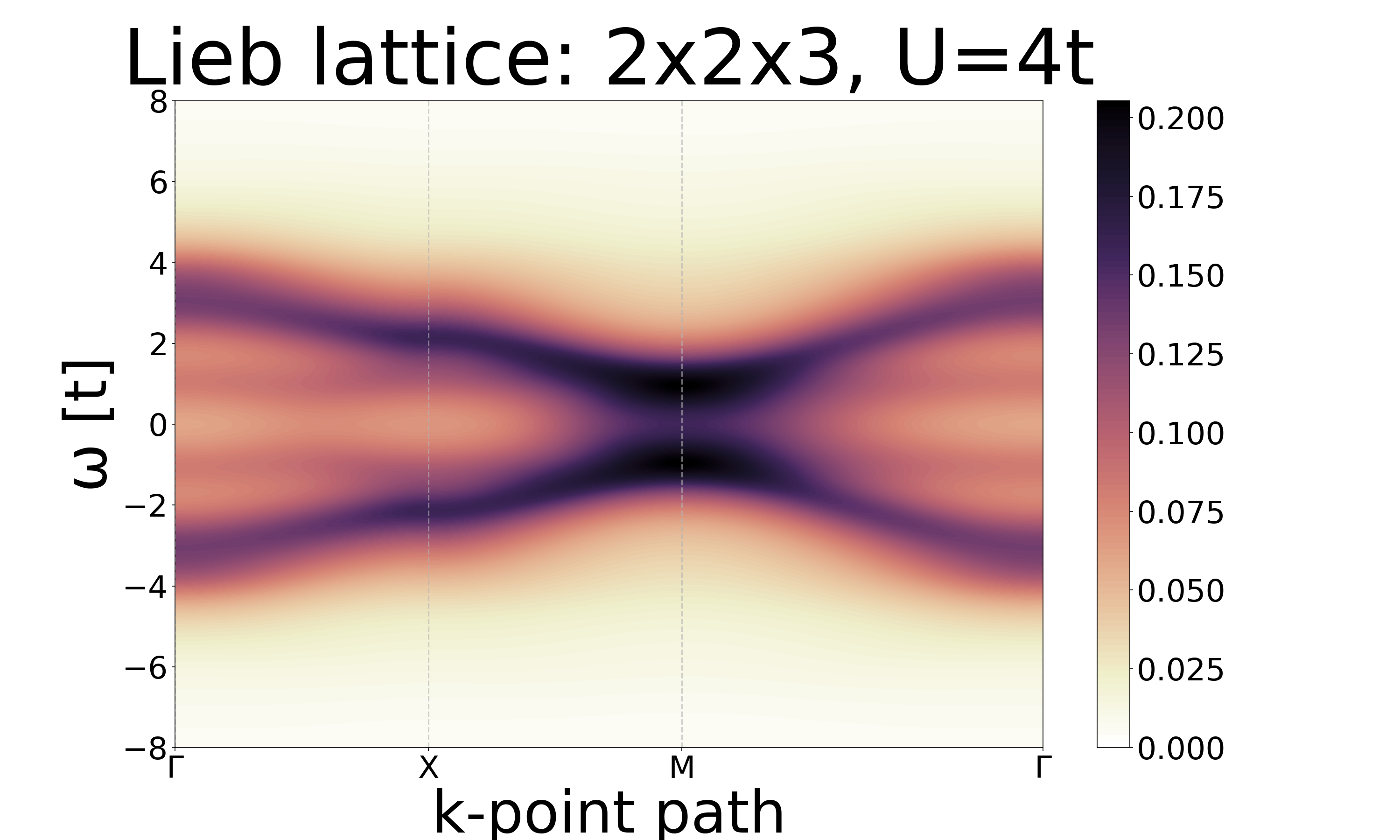
One might now pose the question as to why one should employ CPT in the first place, since all of the reliable information is already contained in the cluster results. To this end, one should realize that just judging from the cluster results it can be very hard to identify how the actual band structure of a system would look like. CPT though, acting as a sort of interpolation scheme between the single particle levels of the cluster and the infinitely large lattice, can give a very good first guess of the band structure, which comes at a negligible additional computational cost. Especially for materials, where short range correlations are predominant, this guess will be highly accurate. Hence one might view it as a useful tool when scanning through a variety of materials. One can simply perform fast CPT calculations for each material, identify interesting band structures and then use more advanced methods to investigate these materials further. As an example, we provide the spectral functions for a more exotic lattice, the Lieb lattice weeks_topological_2010 in Fig. 20 and 21.
IV Conclusion
In this study we have presented fundamental limitations of the CPT method. Most importantly we showed that the cluster Green’s function already contains, as far as interaction effects are concerned, all the information that is included in the CPT Green’s function and CPT only stays consistent with this information. Analysing the 1D case we have shown that the current computational limitations prohibit us to make accurate judgements of features like the Hubbard gap at intermediate interaction strengths, as this would require calculations on larger clusters, as the resolution is limited by the finite size induced level splitting. Additionally and specifically, for the approach of calculating the cluster Green’s function via a Chebyshev expansion, we have shown that Gibbs oscillations require the choice of a large broadening parameter that in return prohibits one from making accurate judgements about the broadness of the peaks in the single particle spectrum. Hence we conclude that use cases for CPT are limited to cases where one is interested in obtaining numerically cheap initial guesses for the spectral function of materials with short range correlations, while more advanced methods need to be employed, to gain higher resolution.
Data availability The data presented in this publication is avaliable on Zenodo under the DOI: 10.5281/zenodo.8063247.
Funding This project was supported by BMBF via the MANIQU grant no. 13N15576.
References
- [1] Ariel Reich and L. M. Falicov. Heavy-fermion system: An exact many-body solution to a periodic-cluster hubbard model. Phys. Rev. B, 37(10):5560–5570, 1988.
- [2] A.-M. S. Tremblay, B. Kyung, and D. Sénéchal. Pseudogap and high-temperature superconductivity from weak to strong coupling. towards quantitative theory. Low Temperature Physics, 32(4):424–451, 2006.
- [3] C. Huscroft, M. Jarrell, Th. Maier, S. Moukouri, and A. N. Tahvildarzadeh. Pseudogaps in the 2d hubbard model. Phys. Rev. Lett., 86(1):139–142, 2001.
- [4] Emanuel Gull, Olivier Parcollet, and Andrew J. Millis. Superconductivity and the pseudogap in the two-dimensional hubbard model. Phys. Rev. Lett., 110(21):216405, 2013.
- [5] Daniel P. Arovas, Erez Berg, Steven A. Kivelson, and Srinivas Raghu. The hubbard model. Annual Review of Condensed Matter Physics, 13(1):239–274, 2022.
- [6] T. Schäfer, F. Geles, D. Rost, G. Rohringer, E. Arrigoni, K. Held, N. Blümer, M. Aichhorn, and A. Toschi. Fate of the false mott-hubbard transition in two dimensions. Phys. Rev. B, 91(12):125109, 2015.
- [7] D. Sénéchal, D. Perez, and M. Pioro-Ladrière. Spectral weight of the hubbard model through cluster perturbation theory. Phys. Rev. Lett., 84(3):522–525, 2000.
- [8] Henrik Bruus and Karsten Flensberg. Many-Body Quantum Theory in Condensed Matter Physics: An Introduction. OUP Oxford, 2004.
- [9] Alexander L Fetter and John Dirk Walecka. Quantum theory of many-particle systems. Courier Corporation, 2012.
- [10] Peter Schmitteckert. Calculating green functions from finite systems. J. Phys.: Conf. Ser., 220:012022, 2010.
- [11] A. Braun and P. Schmitteckert. Numerical evaluation of green’s functions based on the chebyshev expansion. Phys. Rev. B, 90(16):165112, 2014.
- [12] David Sénéchal. An introduction to quantum cluster methods. arXiv:0806.2690 [cond-mat], 2010.
- [13] Eva Pavarini, Erik Koch, Dieter Vollhardt, Alexander I. Lichtenstein, Institute for Advanced Simulation, German Research School for Simulation Sciences, and Deutsche Forschungsgemeinschaft, editors. The LDA+DMFT approach to strongly correlated materials: lecture notes of the Autumn School 2011 Hands-on LDA+DMFT. Number Band 1. 2011.
- [14] Adolfo Avella and Ferdinando Mancini, editors. Strongly Correlated Systems: Theoretical Methods, volume 171 of Springer Series in Solid-State Sciences. Springer Berlin Heidelberg, 2012.
- [15] C. Weeks and M. Franz. Topological insulators on the Lieb and perovskite lattices. Physical Review B, 82(8):085310, August 2010. Publisher: American Physical Society.