Phase-space iterative solvers

Abstract

I introduce a new iterative method to solve problems in small-strain non-linear elasticity. The method is inspired by recent work in data-driven computational mechanics, which reformulated the classic boundary value problem of continuum mechanics using the concept of “phase space”. The latter is an abstract metric space, whose coordinates are indexed by strains and stress components, where each possible state of the discretized body corresponds to a point. Since the phase space is associated to the discretized body, it is finite dimensional. Two subsets are then defined: an affine space termed “physically-admissible set” made up by those points that satisfy equilibrium and a “materially-admissible set” containing points that satisfy the constitutive law. Solving the boundary-value problem amounts to finding the intersection between these two subdomains. In the linear-elastic setting, this can be achieved through the solution of a set of linear equations; when material non-linearity enters the picture, such is not the case anymore and iterative solution approaches are necessary. Our iterative method consists on projecting points alternatively from one set to the other, until convergence. The method is similar in spirit to the “method of alternative projections” and to the “method of projections onto convex sets”, for which there is a solid mathematical foundation that furnishes conditions for existence and uniqueness of solutions, upon which we rely to uphold our new method’s performance. We present two examples to illustrate the applicability of the method, and to showcase its strengths when compared to the classic Newton-Raphson method, the usual tool of choice in non-linear continuum mechanics.

Keywords— Solvers Non-linearity Large systems

List of symbols

Symbol	Meaning	Comment
$n_{e}$	Number of strain/stress components per element
$n_{\text{dofs}}$	Number of nodal degrees of freedom components per node
$N_{n}$	Number of nodes
$N_{e}$	Number of elements
$N_{\text{dofs}}$	Number of degrees of freedom	$=N_{n}\cdot n_{\text{dofs}}$

Symbol	Meaning	Comment
$\boldsymbol{B}_{e}$	Discrete gradient operator	$\in\mathbb{R}^{n_{e}\times N_{\text{dofs}}}$
$\boldsymbol{B}_{e}^{\top}$	Discrete divergence operator	$\in\mathbb{R}^{N_{\text{dofs}}\times n_{e}}$
$\boldsymbol{\sigma}_{e}$	Physically-admissible stress (e-th element)	$\in\mathbb{R}^{n_{e}}$
$\boldsymbol{\varepsilon}_{e}$	Physically-admissible strain (e-th element)	$\in\mathbb{R}^{n_{e}}$
$\boldsymbol{\sigma}^{\prime}_{e}$	Materially-admissible stress (e-th element)	$\in\mathbb{R}^{n_{e}}$
$\boldsymbol{\varepsilon}^{\prime}_{e}$	Materially-admissible strain (e-th element)	$\in\mathbb{R}^{n_{e}}$
$\boldsymbol{m}$	Constitutive-law function	$\boldsymbol{\sigma}^{\prime}_{e}=\boldsymbol{m}(\boldsymbol{\varepsilon}^{\prime}_{e})$
$E$	Physically-admissible set	Equilibrium and compatibility
$P_{E}$	Projection onto $E$
$D$	Materially-admissible set	Constitutive law
$P_{D}$	Projection onto $D$
$Z_{e}$	Local phase space	$\simeq\mathbb{R}^{2n_{e}}$
$Z$	Global phase space	$\simeq\mathbb{R}^{2n_{e}N_{e}}$
$\boldsymbol{z}_{e}$	Point in local phase space	$=\{\boldsymbol{\sigma}_{e},\boldsymbol{\varepsilon}_{e}\}\in Z_{e}$
$\boldsymbol{z}$	Point in global phase space	$=\{[\boldsymbol{z}_{e}]_{e=1}^{N_{e}}\}\in Z$
$\boldsymbol{F}_{int}$	Internal force vector	$\in\mathbb{R}^{N_{\text{dofs}}}$, it depends on stresses
$\boldsymbol{F}_{ext}$	External force vector	$\in\mathbb{R}^{N_{\text{dofs}}}$
$\Delta\boldsymbol{F}$	Force residual	$=\boldsymbol{F}_{int}-\boldsymbol{F}_{ext}$
$\boldsymbol{C}$	Distance constant matrix
$\boldsymbol{K}$	Zero-strain stiffness matrix
$\mathbb{D}$	Zero-strain elastic moduli matrix
$Y$	Young modulus	Function of strain
$Y_{0}$	Zero-strain Young modulus
$\nu$	Poisson’s ratio
$p$	Non-linearity parameter	The larger, the more non-linear the material

1 Introduction

Most practical problems in continuum mechanics lack a simple closed-form solution. Since the advent of modern computers, numerical methods have been developed to overcome this fact and to provide approximate solutions of particular problems for specific values of the relevant parameters [1].

The Newton-Raphson method (NR) has reigned supreme, due to its simplicity, ease of implementation and quadratic convergence [2, 3] (see the appendix for a brief refresh). However, the method is not free from limitations. For once, it requires recomputing the stiffness of the system at every deformation level, what in practical terms means that “tangent stiffness” matrices have to be reassembled at each iteration. This can be time-consuming, and can also entail numerical issues if there are elements in the mesh whose lower stiffness worsens the conditioning of the overall matrix.

A number of alternatives to the Newton-Raphson method have been proposed. Most of them are aimed at minimizing the “force residual”, i.e., the imbalance between internal and external forces, just like NR does, while simultaneously trying to avoid some of its limitations. For instance, quasi-Newton methods approximate successive inverse tangent matrices using the zero-strain stiffness and rank-one corrections by means of Sherman-Morrison formula [4]. Other methods iteratively scan the residual function locally, and search for the optimal direction, and increment, to minimize it. These are termed “search methods” [3, 4], the conjugate gradient method being one of the most popular flavors. Yet another approach, “gradient flow” (a.k.a. “dynamic relaxation”) methods transform the elliptic problem of statics into an auxiliary parabolic problem [4]. This can be solved with time-marching iterations [5] until a steady-state solution is achieved, and that one is then taken to be the solution of the original static problem.

I introduce a new family of iterative solvers for boundary value problems in linear elasticity. The concept of “phase space” introduced in Ref. [6] in the context of data-driven solvers is leveraged. The phase space is $Z=\mathbb{R}^{2n_{e}N_{e}}$, where $N_{e}$ is the number of elements in the mesh and $n_{e}$ is the number of independent components in either the strain or stress tensor in each element. Hence, each coordinate in the phase space corresponds to either a stress or a strain component in an element.

We are implicitly assuming one integration point per element, so stresses and strains are computed at a single location, and that all elements in the mesh are similar (e.g., only 1D bar elements). The global phase space $Z$ can be expressed as the Cartesian product of “local” phase spaces $Z_{e}=\mathbb{R}^{2n_{e}}$ ($e=1,\ldots,N_{e}$), defined at the element level: $Z=Z_{1}\times\ldots\times Z_{N_{e}}$.

Inspired by this seminal work of Kirchdoerfer and Ortiz, we regard the exact solution of the problem as that that satisfies simultaneously boundary conditions, physical balance constraints (in our case Newton’s second law, which boils down to static equilibrium in this case), kinematic considerations (the relation between strains and displacements), and a material-dependent relation between strain and stress. The former two combined defined an affine domain in the global phase space that we term $E$, the “physically-admissible set”. In those authors’ original work, the latter “materially-admissible set” was known as a discrete set of points in the local phase space. In this text, we will assume that, in each element, there is a function $\boldsymbol{m}:\mathbb{R}^{n_{e}}\to\mathbb{R}^{n_{e}}$ that defines a constitutive law $\boldsymbol{\sigma}_{e}^{\prime}=\boldsymbol{m}(\boldsymbol{\varepsilon}_{e}^{\prime})$. As a pivotal assumption, furthermore, we assume that $\{\boldsymbol{\varepsilon}_{e}^{\prime},\boldsymbol{m}(\boldsymbol{\varepsilon}_{e}^{\prime})\}\subset Z_{e}$ defines a curve in $Z_{e}$ that defines limit points of a convex set, and that $\boldsymbol{m}$ is $C^{1}$-continuous.

We term these “phase-space iterative solvers” (PSIs), which include DDCM ones as a particular case in which the constitutive information is known only at discrete points.

The mathematical characterization of this algorithm borrows much from previous work, starting from Von Neumann’s [7, 8] on the methods of alternating projections. His iterative method was shown to be effective to solve large systems of equations [9]. In this context, the method of alternative projections has also been shown to be closely related with the method of subspace corrections [10, 11]. The same philosophy was used to solve a slightly different problem: finding the intersection between convex sets. Convexity happened to be key as it ensured the desired mathematical properties of the method, i.e., convergence, existence and uniqueness. The literature for the method of “projections onto convex sets” (POCS) is extensive, applications [12] ranging from general inverse analysis [13] to image restoration [14, 15].

NR is the alternative that the phase-space iterations’ method has to contend with, so let us advance the advantages with respect to it:

1. Unlike Newton methods, PSI does not require assembling tangent stiffness matrices (or its inverse) at every step; an auxiliary matrix is assembled once, before any iteration, and it is reused later. This matrix is to be chosen by the user, but we will choose $\boldsymbol{K}$, the stiffness matrix at zero strain, throughout this text.

2. Half of the algorithm is trivially parallelizable: solvers like NR that act at the structure level require domain partitions [16, 17, 18] to distribute the work between processors. Setting this up requires meticulous preparation. Conversely, phase-space solvers perform the projection onto the constitutive law element-wise, so this procedure can be divided among processors much more easily, and working on the “local” phase spaces is much less involved than doing so in the “global” one, even though we have to solve a low-dimensionality minimization. The other half of the algorithm is also parallelizable in the sense of classic “domain decomposition” method [19, 20], as it resembles a traditional finite-element algorithm, but in a much more complex manner that requires careful inter-processor communication [16, 21, 22, 23].

3. The distance-minimization method is more general, as it allows handling constitutive laws with less continuity. NR demands derivatives of the constitutive law to be well-defined. But even when that is not the case, we can always solve the distance minimization problem with some of the classic techniques for that purpose (i.e., Brent’s derivative-less method [24]).

2 General formulation

Herein we present the new numerical method, leaving a brief presentation of its main competitor (NR) to the appendix.

2.1 Introduction

Consider a discretized body whose mesh is made up of $N_{n}$ nodes and $N_{e}$ elements, in which each node contains $n_{\text{dofs}}$ degrees of freedom (“dofs”), and stresses and strains are computed at one quadrature point (constant stress elements). In total, there are $N_{\text{dofs}}=n_{\text{dofs}}\times N_{e}$ degrees of freedom, some of them may be constrained while others are free or external forces are applied. Stresses and strains for each element are collected into vectors $\boldsymbol{\sigma}_{e},\,\boldsymbol{\varepsilon}_{e}\in\mathbb{R}^{n_{e}}$, where $n_{e}$ is the minimal number of components to be considered ($n_{e}=1$ for 1D elements, 3 for plane elasticity, 6 for 3D isotropic elasticity and 9 for 3D generalized continua [25]). Thus, each element’s local phase space is isomorphic to $\mathbb{R}^{2n_{e}}$ while the global phase space is to $\mathbb{R}^{2N_{e}n_{e}}$.

We then define a (convex) norm for elements in both the global ($\left\lVert\cdot\right\rVert$) and local ($\left\lVert\cdot\right\rVert_{e}$) phase space:

$$\left\lVert\boldsymbol{z}\right\rVert=\left(\sum_{e=1}^{N_{e}}w_{e}\left\lVert\boldsymbol{z}\right\rVert_{e}^{2}\right)^{1/2}=\left(\sum_{e=1}^{N_{e}}{w_{e}\over 2}\left[\boldsymbol{\varepsilon}_{e}^{\top}\boldsymbol{C}\boldsymbol{\varepsilon}_{e}+\boldsymbol{\sigma}_{e}^{\top}\boldsymbol{C}^{-1}\boldsymbol{\sigma}_{e}\right]\right)^{1/2}\,,$$ (1)

which naturally induces a metric and a distance

$$d(\boldsymbol{z},\boldsymbol{z}^{\prime})=\left\lVert\boldsymbol{z}-\boldsymbol{z}^{\prime}\right\rVert=\left(\sum_{e=1}^{N_{e}}{w_{e}\over 2}\left[(\boldsymbol{\varepsilon}_{e}-\boldsymbol{\varepsilon}_{e}^{\prime})^{\top}\boldsymbol{C}(\boldsymbol{\varepsilon}_{e}-\boldsymbol{\varepsilon}_{e}^{\prime})+(\boldsymbol{\sigma}_{e}-\boldsymbol{\sigma}_{e}^{\prime})^{\top}\boldsymbol{C}^{-1}(\boldsymbol{\sigma}_{e}-\boldsymbol{\sigma}_{e}^{\prime})\right]\right)^{1/2}\,,$$ (2)

where $\boldsymbol{C}$ is a matrix with numbers with proper units so that the two addends are congruent, which is chosen to be both invertible and symmetric. $\boldsymbol{C}$ can be selected by the user, but we will use (a) the zero-strain material moduli, $\boldsymbol{C}=\mathbb{D}$, for the global space distance when projecting onto $E$, (b) a diagonal distance matrix $\boldsymbol{C}=\mathcal{C}\boldsymbol{I}$, for some $\mathcal{C}>0$, for projecting onto $D$.

2.1.1 Physical admissibility

The static equilibrium, in discretized fashion, can be written as

$$\boldsymbol{F}_{int}(\boldsymbol{\sigma})-\boldsymbol{F}_{ext}=\sum_{e=1}^{N_{e}}w_{e}\boldsymbol{B}_{e}^{\top}\boldsymbol{\sigma}_{e}-\boldsymbol{F}_{ext}=0\,,$$ (3)

where $\boldsymbol{F}_{ext}\in\mathbb{R}^{N_{\text{dofs}}}$ is the nodal force vector (containing both external forces and reactions), $w_{e}$ and $\boldsymbol{\sigma}_{e}$ are the volume of each element and its stresses (written as in vector form, i.e., Voigt notation), respectively, while $\boldsymbol{B}_{e}^{\top}\in\mathbb{R}^{N_{\text{dofs}}\times n_{e}}$ is the discrete divergence operator.

Likewise, kinematic compatibility between displacements and infinitesimal strains $\boldsymbol{\varepsilon}_{e}$ (also a vector) in discrete form is

$$\boldsymbol{\varepsilon}_{e}=\boldsymbol{B}_{e}\boldsymbol{u}\,,$$ (4)

where $\boldsymbol{u}$ is the nodal displacement field of that element and $\boldsymbol{B}_{e}\in\mathbb{R}^{n_{e}\times N_{\text{dofs}}}$ is the discrete gradient.

Thus, the first projection will take an initial phase space point satisfying the constitutive law (i.e., $\boldsymbol{z}^{\prime}\in D=\{[(\boldsymbol{\varepsilon}_{e}^{\prime},\boldsymbol{\sigma}_{e}^{\prime})]_{e=1}^{N_{e}}:\boldsymbol{\sigma}_{e}^{\prime}-\boldsymbol{m}(\boldsymbol{\varepsilon}_{e}^{\prime})=0\quad\forall e=1,\ldots,N_{e}\}$) to the closest, in the sense of eq. 22, that belongs in the physically-admissible set, i.e., $\boldsymbol{z}\in E=\{[(\boldsymbol{\varepsilon}_{e}^{\prime},\boldsymbol{\sigma}_{e}^{\prime})]_{e=1}^{N_{e}}:\lx@cref{creftype~refnum}{eq:equilibrium}\}$. This can be expressed as

$$\boldsymbol{z}=P_{E}(\boldsymbol{z}^{\prime})=\mathrm{argmin}\,\Pi_{E}(\cdot,\boldsymbol{z}^{\prime})\,,$$ (5)

where the functional is

$$\Pi_{E}(\boldsymbol{z},\boldsymbol{z}^{\prime})=d_{E}^{2}(\boldsymbol{z},\boldsymbol{z}^{\prime})-\boldsymbol{\eta}\cdot\left(\sum_{e=1}^{N_{e}}w_{e}\boldsymbol{B}_{e}^{\top}\boldsymbol{\sigma}_{e}-\boldsymbol{F}_{ext}\right)\,,$$ (6)

whose stationarity condition, i.e, Euler-Lagrange (E-L) equations [26], verify minimal distance to $\boldsymbol{z}^{\prime}$ subject to equilibrium. The Lagrange multipliers $\boldsymbol{\eta}$ can be thought to represent virtual displacements. We add the subscript $E$ to the distance $d_{E}$ to reiterate that one can use different phase-space norms for $E$ and $D$.

See that compatibility, eq. 4, can be replaced right away wherever $\boldsymbol{\varepsilon}_{e}^{\prime}$ appears, thus the functional $\Pi_{E}$ depends on the field $\boldsymbol{\sigma}_{e}$, $\boldsymbol{\eta}$ (Lagrange multipliers) and $\boldsymbol{u}$ (displacement field).

Let us restate that, in the original DDCM formulation [6], the phase-space distance was the same for both projections, but that does not have to be the case, and actually it will not be the case for us.

2.1.2 Material admissibility

The second projection returns the newly obtained $\boldsymbol{z}\in E$ back to $D$. Unlike the previous one, which is performed at the “mesh” level in the global phase space (involving $\boldsymbol{z}=\{[\boldsymbol{z}_{e}]_{e=1}^{N_{e}}\}$ and $\boldsymbol{z}^{\prime}=\{[\boldsymbol{z}_{e}^{\prime}]_{e=1}^{N_{e}}\}$), the new projection is the collection of $N_{e}$ projections performed at the element level in the local phase spaces. In similar fashion (stretching the notation slightly to use $\boldsymbol{z}^{\prime}$ to denote a new point on $D$), we introduce a new functional, $\Pi_{D_{e}}$, defined element-wise, such that

$$\Pi_{D_{e}}(\boldsymbol{z}_{e}^{\prime},\boldsymbol{z}_{e})=d_{D_{e}}^{2}(\boldsymbol{z}^{\prime}_{e},\boldsymbol{z}_{e})-\boldsymbol{\Lambda}_{e}\cdot\left(\boldsymbol{\sigma}_{e}-\boldsymbol{m}(\boldsymbol{\varepsilon}_{e})\right)\,,$$ (7)

$\boldsymbol{\Lambda}_{e}$ in this case representing virtual strains. Then,

$$\boldsymbol{z}^{\prime}_{e}=\mathrm{argmin}\,\Pi_{D_{e}}(\cdot,\boldsymbol{z}_{e})\,,$$ (8)

which must be solved $N_{e}$ times, one per element (each of those sub-problems i of much less complexity than the global one). Hence, the second projection is defined as

$$\boldsymbol{z}^{\prime}=\{[\boldsymbol{z}_{e}^{\prime}]_{e=1}^{N_{e}}\}=P_{D}(\boldsymbol{z})=\{[\mathrm{argmin}\,\Pi_{D_{e}}(\cdot,\boldsymbol{z}_{e})]_{e=1}^{N_{e}}\}\,.$$ (9)

2.1.3 Consecutive iterations

We envision an iterative method, geometric in nature, in which each iteration consists of two projections. After the two projections, the point obtained at the prior iteration (say, $\boldsymbol{z}^{\prime(n)}$) yields $\boldsymbol{z}^{\prime(n+1)}=P_{D}P_{E}(\boldsymbol{z}^{\prime(n)})$. The method, under some conditions, is guaranteed to converge in norm, in the sense that the distance $\left\lVert(P_{D}P_{E})^{k+1}\boldsymbol{z}_{0}-(P_{D}P_{E})^{k}\boldsymbol{z}_{0}\right\rVert\to 0$ as $k\to\infty$. See that the convergence of the method in this manner does not automatically imply that the force residual (i.e., the difference between external and internal forces) goes to zero in the same way. This is a remarkable difference when comparing to most solid mechanics solvers, which tend to be predicated in the minimization of the latter. For this reason, it is logical that PSI solvers may be equipped with a dual stop condition, which simultaneously checks both “phase-space convergence” (in terms of phase-space distance between iterations becoming smaller) and “equilibrium convergence” (in terms of force residual).

The solution procedure is as follows:

1. Choose a point $\boldsymbol{z}^{\prime(0)}\in Z$ that satisfies the constitutive laws defined at each element level, or simplify starting from the origin (which is part of the constitutive law).

2. Apply $\boldsymbol{z}^{\prime(k)}=(P_{D}P_{E})^{k}(\boldsymbol{z}^{\prime(0)})$ until either

   • (a) $\left\lVert\boldsymbol{F}_{int}(\boldsymbol{\sigma}^{\prime})-\boldsymbol{F}_{ext}\right\rVert_{L^{2}}<\mathrm{tol}_{1}\left\lVert\boldsymbol{F}_{ext}\right\rVert_{L^{2}}$, or

   • (b) $\left\lVert\boldsymbol{z}^{\prime(k)}-\boldsymbol{z}^{\prime(k-1)}\right\rVert<\mathrm{tol}_{2}\left\lVert\boldsymbol{z}^{\prime(k-1)}\right\rVert$.

Later in this text, we will argue that $\mathrm{tol}_{1}>\mathrm{tol}_{2}$; in particular, we shall show that $\mathrm{tol}_{2}=\mathrm{tol}_{1}/10$ to be a satisfactory choice.

2.2 Operative form of the projections

2.2.1 Projection onto $E$

Assume given $\boldsymbol{z^{\prime}}=\{(\boldsymbol{\varepsilon}_{e}^{\prime},\boldsymbol{\sigma}_{e}^{\prime})_{e=1}^{N_{e}}\}$. Enforcing the stationarity condition ($\delta\Pi_{E}=0$) to obtain, field by field,

$$\delta\boldsymbol{u} \to\sum_{e=1}^{N_{e}}w_{e}\boldsymbol{B}_{e}^{\top}\boldsymbol{C}(\boldsymbol{B}_{e}\boldsymbol{u}-\boldsymbol{\varepsilon}_{e}^{\prime})=0\to\left(\sum_{e=1}^{N_{e}}w_{e}\boldsymbol{B}_{e}^{\top}\boldsymbol{C}\boldsymbol{B}_{e}\right)\boldsymbol{u}=\sum_{e=1}^{N_{e}}w_{e}\boldsymbol{B}_{e}^{\top}\boldsymbol{C}\boldsymbol{\varepsilon}_{e}^{\prime}\,,$$ (10a)

$$\delta\boldsymbol{\sigma}_{e} \to w_{e}\boldsymbol{C}^{-1}\left(\boldsymbol{\sigma}_{e}-\boldsymbol{\sigma}_{e}^{\prime}\right)-w_{e}\boldsymbol{B}_{e}\boldsymbol{\eta}=0\to\boldsymbol{\sigma}_{e}=\boldsymbol{\sigma}_{e}^{\prime}+\mathcal{C}\boldsymbol{B}_{e}\boldsymbol{\eta}\,,$$ (10b)

$$\delta\boldsymbol{\eta} \to\sum_{e=1}^{N_{e}}w_{e}\boldsymbol{B}_{e}^{\top}\sigma_{e}-\boldsymbol{F}_{ext}=0\,.$$ (10c)

Upon combination of eq. 10b with eq. 10c, one obtains:

$$\left(\sum_{e=1}^{N_{e}}w_{e}\boldsymbol{B}_{e}^{\top}\boldsymbol{C}\boldsymbol{B}_{e}\right)\boldsymbol{\eta}=\boldsymbol{K}\boldsymbol{\eta}=\boldsymbol{F}_{ext}-\sum_{e=1}^{N_{e}}w_{e}\boldsymbol{B}_{e}^{\top}\sigma_{e}^{\prime}=\boldsymbol{F}_{ext}-\boldsymbol{F}_{int}$$

$$\to\boldsymbol{K}\boldsymbol{\eta}=\boldsymbol{F}_{ext}-\boldsymbol{F}_{int}(\boldsymbol{\sigma}^{\prime})=\Delta\boldsymbol{F}(\boldsymbol{\sigma}^{\prime})\,,$$ (11)

wherefrom it becomes apparent that $\boldsymbol{\eta}$ can be understood as a measure of the imbalance between external forces and internal forces for a pre-assumed value of materially-admissible stresses $\boldsymbol{\sigma}^{\prime}$. In practice, the equation is solved only for those degrees of freedom that come not imposed by BCs. For the latter, it is set from the start that $\eta_{i}=0$. Once the nodal imbalance variables $\boldsymbol{\eta}$ are available, from eq. 10b we find

$$\boldsymbol{\sigma}_{e}=\boldsymbol{\sigma}_{e}^{\prime}+\boldsymbol{C}\boldsymbol{B}_{e}\boldsymbol{K}^{-1}\left(\boldsymbol{F}_{ext}-\boldsymbol{F}_{int}(\boldsymbol{\sigma}^{\prime})\right)\,,$$ (12)

for each element.

The essential boundary conditions must be enforced as part of finding the physically-admissible solution. We can set another system of linear equations from eq. 10a

$$\boldsymbol{K}\boldsymbol{u}=\sum_{e=1}^{N_{e}}w_{e}\boldsymbol{B}_{e}^{\top}\boldsymbol{C}\boldsymbol{\varepsilon}^{\prime}\,,$$ (13)

and then enforce the essential BCs ($u_{i}=\hat{u}_{i}$) for some prescribed value $\hat{u}_{i}$ . In the current version of the code, this is done by “condensing” the imposed displacements, substituting them directly into the vector $\boldsymbol{u}$ and solving eq. 13 for a reduced system that includes the “free” degrees of freedom and forces arising from condensation [1, 5].

Summarizing, the first projection goes from $\boldsymbol{z}^{\prime}=\{[(\boldsymbol{\varepsilon}^{\prime}_{e},\boldsymbol{\sigma}_{e}^{\prime})]_{e=1}^{N_{e}}\}\in D$ to

$$\boldsymbol{z} =\{[(\boldsymbol{\varepsilon}_{e},\boldsymbol{\sigma}_{e})]_{e=1}^{N_{e}}\}=P_{E}(\boldsymbol{z}^{\prime})=\{[(\boldsymbol{\varepsilon}^{\prime}_{e},\boldsymbol{\sigma}_{e}^{\prime})]_{e=1}^{N_{e}}\}$$

$$=\{[\boldsymbol{B}_{e}\boldsymbol{K}^{-1}\sum_{e=1}^{N_{e}}w_{e}\boldsymbol{B}_{e}^{\top}\boldsymbol{C}\boldsymbol{\varepsilon}^{\prime},\boldsymbol{\sigma}_{e}^{\prime}+\boldsymbol{C}\boldsymbol{B}_{e}\boldsymbol{K}^{-1}\Delta\boldsymbol{F}(\boldsymbol{\sigma}^{\prime})]_{e=1}^{N_{e}}\}\in E\,.$$ (14)

See that the matrix $\boldsymbol{K}$ could be anything, depending on the choice of $\boldsymbol{C}$. For instance, when $\boldsymbol{C}=\mathbb{D}$, $\boldsymbol{K}$ becomes the tangent matrix at the origin, which is computed and stored once and needs no updating across iterations.

2.2.2 Projection onto $D$

Assume given $\boldsymbol{z}=\{(\boldsymbol{\varepsilon}_{e},\boldsymbol{\sigma}_{e})_{e=1}^{N_{e}}\}$. When it comes to the projection over the constitutive law, the stationarity condition for eq. 7 yield the following E-L equations

$$\delta\boldsymbol{\varepsilon}_{e}^{\prime} \to\boldsymbol{C}\left(\boldsymbol{\varepsilon}_{e}^{\prime}-\boldsymbol{\varepsilon}_{e}\right)+\boldsymbol{\Lambda}_{e}\nabla\boldsymbol{m}(\boldsymbol{\varepsilon}_{e}^{\prime})=0\to\boldsymbol{\varepsilon}_{e}^{\prime}=\boldsymbol{\varepsilon}_{e}-\boldsymbol{C}^{-1}\boldsymbol{\Lambda}_{e}\nabla\boldsymbol{m}(\boldsymbol{\varepsilon}_{e}^{\prime})\,,$$ (15a)

$$\delta\boldsymbol{\sigma}_{e}^{\prime} \to\boldsymbol{C}^{-1}\left(\boldsymbol{\sigma}_{e}^{\prime}-\boldsymbol{\sigma}_{e}\right)-\boldsymbol{\Lambda}_{e}=0\to\boldsymbol{\Lambda}_{e}=\boldsymbol{C}^{-1}\left(\boldsymbol{\sigma}_{e}^{\prime}-\boldsymbol{\sigma}_{e}\right)\,,$$ (15b)

$$\delta\boldsymbol{\Lambda}_{e} \to\boldsymbol{\sigma}_{e}^{\prime}-\boldsymbol{m}(\boldsymbol{\varepsilon}_{e}^{\prime})=0\to\boldsymbol{\sigma}_{e}^{\prime}=\boldsymbol{m}(\boldsymbol{\varepsilon}_{e}^{\prime})\,.$$ (15c)

Enough continuity has to be assumed so that the gradient of the constitutive law ($\nabla\boldsymbol{m}$) is well-defined. See that we can minimize the distance directly, thorough some numerical approach, after enforcing the constitutive law relation eq. 15c. We will do so, further simplifying the setting by assuming a diagonal matrix for the distance coefficients, i.e., $\boldsymbol{C}=\mathcal{C}\boldsymbol{I}$, hence

$$\boldsymbol{z}_{e}^{\prime}=\mathrm{argmin}\,\bar{\Pi}_{D}=\mathrm{argmin}\left\{{\mathcal{C}\over 2}(\boldsymbol{\varepsilon}_{e}^{\prime}-\boldsymbol{\varepsilon}_{e})\cdot(\boldsymbol{\varepsilon}_{e}^{\prime}-\boldsymbol{\varepsilon}_{e})+{1\over 2\mathcal{C}}(\boldsymbol{m}(\boldsymbol{\varepsilon}_{e}^{\prime})-\boldsymbol{\sigma}_{e})\cdot(\boldsymbol{m}(\boldsymbol{\varepsilon}_{e}^{\prime})-\boldsymbol{\sigma}_{e})\right\}\,.$$ (16)

Minimizing this distance is precisely the traditional approach in DDCM [6], but notice that in this case, since $\boldsymbol{m}(\varepsilon_{e}^{\prime})$ is known, one does not have to scan a discrete dataset, but functional minimization of the objective function, based on its derivatives or not, can be leveraged to find the minimizer directly, dodging the need for Euler-Lagrange equations.

Conversely, combining eqs. 15a, 15b and 15c yields a non-linear vector equation for $\boldsymbol{\varepsilon}_{e}^{\prime}$:

$$\boldsymbol{\varepsilon}_{e}^{\prime}=\boldsymbol{\varepsilon}_{e}+\boldsymbol{C}^{-1}\boldsymbol{C}^{-1}(\boldsymbol{\sigma}_{e}-\boldsymbol{m}(\boldsymbol{\varepsilon}_{e}^{\prime}))\nabla\boldsymbol{m}(\boldsymbol{\varepsilon}_{e}^{\prime})=\boldsymbol{\varepsilon}_{e}+{(\boldsymbol{\sigma}_{e}-\boldsymbol{m}(\boldsymbol{\varepsilon}_{e}^{\prime}))\over\mathcal{C}^{2}}\nabla\boldsymbol{m}(\boldsymbol{\varepsilon}_{e}^{\prime})\,.$$ (17)

This equation is referred to as “the Euler-Lagrange equation of $P_{D}$” hereafter, as it combines eqs. 15a, 15b and 15c into one. It represents a vector equation whose complexity depends on the form of the function $\boldsymbol{m}$, and on the number of components of the vectors ($n_{e}$), which depends on the problem: for instance, 3 components for plane stress or strain, and for 1D-element meshes it boils down to a scalar equation.

Algorithm 1 Phase-space iterative projections

Require: Connectivity, $\forall e=1,\ldots,N_{e}$, compatibility matrices $\boldsymbol{B}_{e}$; zero-strain moduli’s matrix $\mathbb{D}$; matrix of distance constants $\boldsymbol{C}$; $\forall i=1,\ldots,N_{\text{dof}}$, external forces $F_{ext}$ or boundary conditions.

(i) Set $k=0$. Initial data assignation:

for $e=1,\ldots,N_{e}$  do

     Set $\boldsymbol{z^{\prime}}_{e}^{(0)}=(0,0)$, unless there being essential boundary conditions in the nodes of the said element, in that case set $\boldsymbol{\varepsilon}_{e}^{\prime}=\boldsymbol{B}_{e}\hat{\boldsymbol{u}}$.

end for

(ii) Project onto $\mathrm{E}$:

Given $\boldsymbol{z^{\prime}}^{(k)}$, find $\boldsymbol{z}^{(k+1)}=\{\boldsymbol{z}_{e}^{(k+1)}\}_{e=1}^{N}=\{(\varepsilon_{e},\sigma_{e})\}_{e=1}^{N}$ from solving eq. 10 to get $\boldsymbol{u}^{(k+1)}$ and $\boldsymbol{\eta}^{(k+1)}$

for $e=1,\ldots,N_{e}$  do

     Compute $\boldsymbol{\varepsilon}_{e}$ from eq. 4 and $\boldsymbol{\sigma}_{e}$ from eq. 12

end for

(iii) Project onto $\mathrm{D}$:

for $e=1,\ldots,N_{e}$  do

     Given $\boldsymbol{z}^{(k+1)}=\{\boldsymbol{z}^{(k+1)}_{e}\}_{e=1}^{N}$, find $\boldsymbol{z^{\prime}}^{(k+1)}_{e}=(\boldsymbol{\varepsilon}^{\prime}_{e},\boldsymbol{\sigma}^{\prime}_{e})$, where $\boldsymbol{\varepsilon}^{\prime}_{e}$ is got from eq. 16 and then $\boldsymbol{\sigma}^{\prime}_{e}=\boldsymbol{m}(\boldsymbol{\varepsilon}^{\prime}_{e})$.

end for

(iv) Convergence test:

if  $\boldsymbol{K}\boldsymbol{\eta}^{(k+1)}<\mathrm{tol}_{1}\left\lVert\boldsymbol{F}_{ext}\right\rVert_{L^{2}}$ then

     Final displacement field $\boldsymbol{u}=\boldsymbol{u}^{(k+1)}$ exit

else if $\left\lVert\boldsymbol{z}^{(k+1)}-\boldsymbol{z}^{(k)}\right\rVert<\mathrm{tol}_{2}\left\lVert\boldsymbol{z}^{(k)}\right\rVert$

     Final displacement field $\boldsymbol{u}=\boldsymbol{u}^{(k+1)}$ exit

else

     $k\leftarrow k+1$, goto (ii)

end if

3 2D plane-strain example: plate with hole

We resort to a 2D benchmark exercise: a thick square plate (side length $L=0.2\,\mathrm{m}$) with a circular hole (radius $r=0.02\,\mathrm{m}$) loaded in tension on two opposite edges, see Figure 1(a). The applied traction $\sigma_{0}$ equals $100\,\mathrm{MPa/m}$.

The material the plate is made of is assumed to lose stiffness with increasing mean strain ($\varepsilon_{m}=(\varepsilon_{\text{I}}+\varepsilon_{\text{II}}+\varepsilon_{\text{III}})/3=(\varepsilon_{\text{xx}}+\varepsilon_{\text{yy}})/3$). No inelastic behavior is considered in these simulations. The Young’s modulus of the material is assumed to change according to (Figure 1(b)), thus:

$$\boldsymbol{\sigma}=\mathbb{D}(\varepsilon_{m})\boldsymbol{\varepsilon}={Y(\varepsilon_{m})\over(1+\nu)(1-2\nu)}\begin{bmatrix}1-\nu&\nu&0\\ \nu&1-\nu&0\\ 0&0&{1-2\nu\over 2}\end{bmatrix}\boldsymbol{\varepsilon}\,,$$ (18)

where

$$Y(x)=pY_{0}(|x|+c)^{p-1}\,,$$ (19)

$Y_{0}$ being the zero-strain modulus. The Poisson’s ratio is assumed to remain constant. For the simulations we are to show, $Y_{0}=200\,\mathrm{GPa}$, $\nu=0.33$.

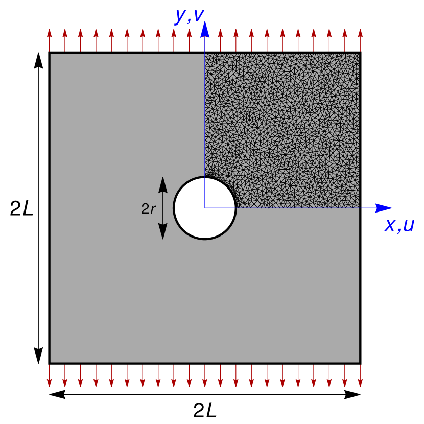
(a) (a)

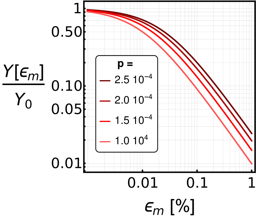
(b) (b)

Figure 1: System geometry and material. (a) Scheme of the system, including loading and reduced mesh (taking advantage of symmetry). (b) Young modulus as a function of mean strain for different values of $p$.

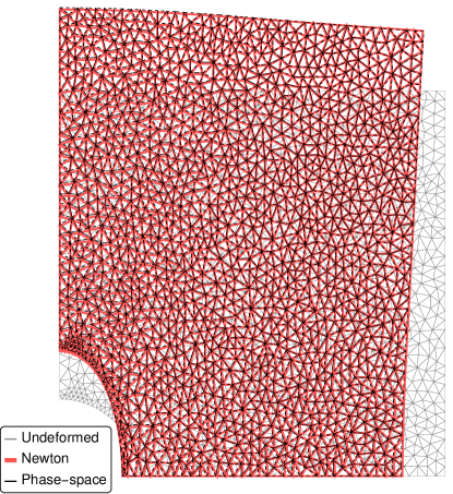
Figure 2: Results: deformation with both methods ($\times 250$ magnification), material corresponding to $p=2\cdot 10^{-4}$.

The mesh is generated with constant-stress triangular elements (CSTs).

The total external force is applied over one step, and NR’s convergence condition is $\left\lVert\boldsymbol{F}_{int}(\boldsymbol{\sigma}^{\prime})-\boldsymbol{F}_{ext}\right\rVert_{L^{2}}<0.01\left\lVert\boldsymbol{F}_{ext}\right\rVert_{L^{2}}$. Thus, $\mathrm{tol}_{1}=0.01$; for the PSI, the computation can also stop if $\left\lVert\boldsymbol{z}^{\prime(k)}-\boldsymbol{z}^{\prime(k-1)}\right\rVert<0.001\left\lVert\boldsymbol{z}^{\prime(k-1)}\right\rVert$, i.e., $\mathrm{tol}_{2}=\mathrm{tol}_{1}/10$.

See Figure 3 for a partial depiction of phase-space projections. When properly solved (i.e., in absence of numerical artifacts), both methods yield the same solution, see Figure 2.

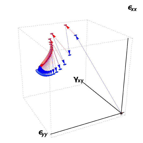
Figure 3: Local phase-space iterations for a particular element (showing only strain components). Blue (red) arrows represent successive projections onto $E$ ($D$).

In the following sections, I will consider the influence of different parameters on the performance of the method.

3.1 Changing the distance function: influence of $\mathcal{C}$

I first explore the influence of the distance function used. This is tantamount to changing the constants that appear in eq. 2 for the projection $P_{D}$, since we have established from the get-go that for $P_{E}$ the constant matrix is $\boldsymbol{C}=\mathbb{D}$, so the projection matrix $\boldsymbol{K}$ is the zero-strain stiffness matrix. For simplicity, we chose $\boldsymbol{C}=\mathcal{C}\boldsymbol{I}$, rendering eq. 16, and express it as ratio with respect to the zero-strain Young modulus, i.e., $\mathcal{C}/Y_{0}$.

This minimization problem has to be solved element by element. For now, we will use Brent’s derivative-less method [24] and four CPUs (kernels) to perform the projections onto the constitutive law. We are using Mathematica’s function FindMinimum with default parameters, providing the previous physically-admissible strain ($\boldsymbol{\varepsilon}_{e}$) as starting point to the search.

For $p=2.5\cdot 10^{-4}$, see Table 1. Both $\mathcal{C}/Y_{0}=0.01$ and $\mathcal{C}/Y_{0}=10$ converge quickly in phase-space distance ($\mathrm{tol}_{2}$) but with $95\%$ error $\mathrm{tol}_{1}$, i.e., equilibrium far from being satisfied even though the phase space distance converged. That is why they are not even shown in the table.

Table 1: Wallclock time comparisons using distance minimization for $P_{D}$. Material defined by $p=2.5\cdot 10^{-4}$. Using $\mathcal{C}=0.1Y_{0}$. Mesh made up by 2872 CST elements.

	Newton-Raphson solver	Phase-space iterative solver
		$\mathcal{C}=0.1$	$\mathcal{C}=1.0$
Running time [s]	8.25	8.30	26.10

3.2 How does non-linearity affect relative performance?

We observe that PSI fares better than NR when most material response is non-linear, i.e., low value of $p$ (see Table 2). This is attributed to PSI enforcing the constitutive law during a dedicated step ($P_{D}$) and element-wise, while NR enforces equilibrium and the constitutive law simultaneously when solving the residual equations. NR relies on the tangent stiffness matrix, so there being elements that accumulate deformation can lead to entries of disparate magnitude and poor conditioning of the matrices.

Table 2: Wallclock time comparisons using distance minimization for $P_{D}$. Using $\mathcal{C}=0.1Y_{0}$. Mesh made up by 2872 CST elements. Asterisk (^∗) on PSI results to stress that $\mathrm{tol}_{2}$ was met before $\mathrm{tol}_{1}$.

	Degree of non-linearity, $p/10^{-4}$
	2.5 (stiff)	2.0	1.5 (compliant)
NR running time [s]	8.25	9.96	93.10
PSI running time [s]	8.48	15.29	33.97∗

Table 2 suggests that PSI can be especially competitive when it comes to finding approximate solutions of problems featuring widespread non-linear behavior. The ^∗ denotes that the calculation ends because of $\mathrm{tol}_{2}$ (phase-space convergence), $\mathrm{tol}_{1}$ is not met (equilibrium tolerance), the final equilibrium error being $2.6\%$, i.e., the final stresses satisfy $\left\lVert\boldsymbol{F}_{int}(\boldsymbol{\sigma}^{\prime})-\boldsymbol{F}_{ext}\right\rVert_{L^{2}}=0.026\left\lVert\boldsymbol{F}_{ext}\right\rVert_{L^{2}}$. I observe that when $\mathrm{tol}_{2}=\mathrm{tol}_{1}/10$, if the method converges first in phase-space distance, it always yields also a small force residual, less than $4\%$, despite not reaching the more constrained target.

3.3 Influence of number of kernels

Table 3 shows the impact of parallelizing $P_{D}$, the element-by-element projections onto the material set. The scaling is good up to four kernels, at which point it saturates. This seems to be due to limitations in the parallelization strategy employed by the software where computations are carried out (Mathematica).

Table 3: Wallclock time comparisons using distance minimization for $P_{D}$. Material defined by $p=2.0\cdot 10^{-4}$. Using $\mathcal{C}=0.1Y_{0}$. Mesh made up by 2872 CST elements.

	Newton-Raphson solver	Phase-space iterative solver
		serial	2 kernels	4 kernels	8 kernels
Running time [s]	9.96	43.47	25.50	15.29	14.08

3.4 Distance minimization: method comparison

Another advantage of the PSI solver is its adaptability when it comes to choosing an approach to numerically minimize the distance in eq. 16. We have tried four different methods, three that rely on derivatives of the objective function (Newton, quasi-Newton and conjugate gradient [2]) and one that does not (Brent’s principal axis [24]). For this example, the derivative-less method is about a 50% slower, but this situation will reverse when considering simpler local phase spaces.

Table 4: Wallclock time comparisons using distance minimization for $P_{D}$ (different methods). Material defined by $p=2.0\cdot 10^{-4}$. Using $\mathcal{C}=0.1Y_{0}$. Mesh made up by 2872 CST elements.

	Principal Axis (derivative-free)	Conjugate gradient	Quasi-Newton	Newton
Running time [s]	15.29	10.60	10.70	10.82

3.5 Performance as function of mesh size

The effect of refining the mesh is examined next. The original mesh features 2872 CST elements, corresponding to a target triangle length $\ell=0.5\,\mathrm{cm}=L/20$ ($2L$ is the length of the plate, Figure 1(a)). Reducing to $\ell/L=1/33.33$ and $\ell/L=1/50$ yields 7881 and 17540, respectively. In the 2D setting, the number of elements scale quadratically with the element length, i.e., reducing the side length by a factor $\ell_{2}/\ell_{1}$ yields a mesh containing approximately $(\ell_{2}/\ell_{1})^{2}$ times the starting number of elements.

Table 5 shows a remarkable scaling of PSI, significantly better than NR’s. As the mesh is refined, the number of elements and degrees of freedom to consider also increases. For NR, this means substantially larger sparse matrices to handle: the size of the tangent matrix also scales quadratically with the characteristic element size. Contrariwise, for PSI, it only means more independent resolutions of eq. 16. Consequently, the running time appears to scale linearly with the number of elements.

Note that, if the scaling with the number of processors was optimal, doubling the number of processors would cancel the time increase associated to doubling the number of elements in the mesh.

Table 5: Wallclock time comparisons using distance minimization for $P_{D}$. Using $\mathcal{C}=0.1Y_{0}$.

	# elements
	2872	7881	17540
NR running time [s]	7.73	39.16	158.93
PSI running time [s]	8.30	21.04	54.5

3.5.1 Plate without hole

Interestingly enough, simplifying the geometry of the system also has a strong impact over the performance of PSI. We re-run the plate simulation but removing the hole from its midst, recall that we set $\mathrm{tol}_{2}=\mathrm{tol}_{1}/10=10^{-3}$.

NR still suffers from the same difficulties associated to having to handle ever-larger matrices. It is acknewledged that for this simpler geometry and the two smaller meshes, PSI converged in phase-space norm in just two iterations, while having a relatively small residual ($3.73\%$ instead of the target $1\%$). I reckon that the convergence is faster when the stress state is simpler: removing the hole also removes the need to find/project over complex stress/deformation states.

Table 6: Plate without hole. Wallclock time comparisons using distance minimization for $P_{D}$. Material $p=2\cdot 10^{-4}$. Using $\mathcal{C}=0.1Y_{0}$, distance minimization (conjugate gradient) and 4 kernels. In parentheses, the final residual error. Asterisk (^∗) on PSI results to stress that $\mathrm{tol}_{2}$ was met before $\mathrm{tol}_{1}$.

	# elements
	728 ($3.73\%$)	2886 ($3.73\%$)	11708 ($1.00\%$)
NR running time [s]	0.58	4.88	95.4
PSI running time [s]	0.42∗	1.33∗	8.66

4 1D-elements in 3D space: Kirchdoerfer’s truss

The special interest of this application is to work with the simplest phase-space possible. We have found, particularly, the projection onto the materially-admissible set using the Euler-Lagrange equations to be more efficient in this context, both in terms of implementation and actual performance. This simple setting allows us to explore also the possibility of introducing an “optimal” distance function [27].

The structure we focus on is “Kirchdoerfer’s truss”, a simple truss system introduced in [6]. It features 1246 elements and 1128 nodes. The non-linear elastic law presented in [6] is equipped on all the elements, and it is given by

$$\sigma=m(\varepsilon)=Y_{0}\left[(|\varepsilon|+c)^{p}-c^{p}\right]\mathrm{sign}(\varepsilon)\,,$$ (20)

where $c=p^{(1-p)^{-1}}$, $Y_{0}$ represents the axial stiffness at zero strain, $|\cdot|$ is the absolute value function and $\mathrm{sign}(\cdot)$ is the sign function. See Figure 4(b). In this example, $Y_{0}=200\mathrm{GPa}$ and $p$ will be changed from $5\cdot 10^{-5}$ to $5\cdot 10^{-4}$.

We compare the new solver to a damped Newton-Raphson (see appendix), which is more adequate to handle the forced displacement conditions. We will use a damping parameter of $0.8$, i.e., the zero-strain stiffness is 20% of each iteration stiffness matrix.

4.1 Simplifying the formulation for 1D elements

By virtue of the typology of the connection among bar elements, they work primarily by stretching, so the mechanical state of the $e$-th element corresponds to the simplest local phase space, i.e., $Z_{e}=\mathbb{R}^{2}$ ($n_{e}=1$), each point defined by only two coordinates $(\sigma_{e},\varepsilon_{e})$.

Let us particularize Section 2 for this the simplest phase space. In this case, the norms and distances simplify considerably:

$$\left\lVert\boldsymbol{z}\right\rVert=\left(\sum_{e=1}^{N_{e}}w_{e}\left\lVert\boldsymbol{z}\right\rVert_{e}^{2}\right)^{1/2}=\left(\sum_{e=1}^{N_{e}}w_{e}\left[{\varepsilon_{e}^{2}\over 2\mathcal{C}^{-1}}+{\sigma_{e}^{2}\over 2\mathcal{C}}\right]\right)^{1/2}\,,$$ (21)

which naturally induces a metric and a distance

$$d(\boldsymbol{z},\boldsymbol{z}^{\prime})=\left\lVert\boldsymbol{z}-\boldsymbol{z}^{\prime}\right\rVert=\left(\sum_{e=1}^{N_{e}}w_{e}\left[{(\sigma_{e}-\sigma_{e}^{\prime})^{2}\over 2\mathcal{C}}+{(\varepsilon_{e}-\varepsilon_{e}^{\prime})^{2}\over 2\mathcal{C}^{-1}}\right]\right)^{1/2}\,,$$ (22)

where $\mathcal{C}$ is but a number with proper units so that the two addends are congruent. For $P_{E}$, I shall use $\mathcal{C}=Y_{0}$, while for $P_{D}$, the “optimal” value will be used.

The projection onto $E$ does nor change qualitatively, but when it comes to $D$ (enforcing the constitutive law relation), we obtain a different expression in which inner products (norms) do not appear:

$$\boldsymbol{z}_{e}^{\prime}=\mathrm{argmin}\,\bar{\Pi}_{D}=\mathrm{argmin}\left\{{(\varepsilon_{e}^{\prime}-\varepsilon_{e})^{2}\over 2\mathcal{C}^{-1}}+{(m(\varepsilon_{e}^{\prime})-\sigma_{e})^{2}\over 2\mathcal{C}}\right\}\,.$$ (23)

and the Euler-Lagrange equation, similarly to eq. 17, yields

$$\varepsilon_{e}^{\prime}=\varepsilon_{e}+{(\sigma_{e}-m(\varepsilon_{e}^{\prime}))\over\mathcal{C}^{2}}{dm(\varepsilon_{e}^{\prime})\over d\varepsilon_{e}^{\prime}}\,.$$ (24)

We can consider the metric constant $\mathcal{C}$ as an independent field in eq. 23, and take variations with respect to it [27]:

$$\delta\mathcal{C} \to{(\varepsilon_{e}^{\prime}-\varepsilon_{e})^{2}\over 2}-{(m(\varepsilon_{e}^{\prime})-\sigma_{e})^{2}\over 2\mathcal{C}^{2}}=0\to\mathcal{C}^{*}={m(\varepsilon_{e}^{\prime})-\sigma_{e}\over\varepsilon_{e}^{\prime}-\varepsilon_{e}}\,.$$ (25)

Using this optimal value

$$\boldsymbol{z}_{e}^{\prime}=\mathrm{argmin}\,\bar{\Pi}_{D}^{\text{{opt}}}=\mathrm{argmin}\left\{(\varepsilon_{e}^{\prime}-\varepsilon_{e})(m(\varepsilon_{e}^{\prime})-\sigma_{e})\right\}\,.$$ (26)

The stationarity condition for this functional yields

$$\varepsilon_{e}^{\prime}=\varepsilon_{e}+{(\sigma_{e}-m(\varepsilon_{e}^{\prime}))\over dm(\varepsilon_{e}^{\prime})/d\varepsilon_{e}^{\prime}}\,,$$ (27)

where the gradient appears in the denominator, unlike in eqs. 17 and 24.

(a) (a)

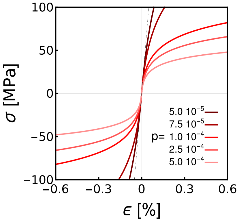
(b) (b)

Figure 4: Truss example. (a) Structure: red arrows indicate applied forces, blue ones correspond to imposed displacements. (b) Constitutive law used for the all bars in the truss.

4.2 Detailed analysis of one run

The material model corresponds to $p=10^{-4}$, see Figure 4(b). The tolerance is initially set to be $\mathrm{tol}_{1}=5\cdot 10^{-2}=5\%$. We employ the optimal phase-space distance for projections onto $D$, i.e., we are using Mathematica’s function FindRoot to solve eq. 27, with Newton’s method, step control (“trust region”) and computing the necessary Jacobians with finite differences, while also providing the previous physically-admissible strain ($\boldsymbol{\varepsilon}_{e}$) as starting point to the search.

4.2.1 Using Euler-Lagrange equation (optimal distance)

For a single run, the NR solver took $2.52\,\mathrm{s}$ and 27 iterations to achieve the desired tolerance. Conversely, PSI converged after 13 iterations (each iteration here concerns two projections) in $2.11\,\mathrm{s}$, employing eight parallel processors to perform the projections onto the constitutive law.

Qualitatively, Figure 5(a) reveals that the NR solver initial guess leads to a large initial residual , due to inclusion of forced displacements into the initial guess (this is a well-known difficulty). This imbalance is brushed away over subsequent iterations, and the solver converges much quicker (quadratically) in the surroundings of the solution. Conversely, the PSI solution starts from zero initial forces, as we set $\boldsymbol{z^{\prime}}^{(0)}=\boldsymbol{0}$. The driving force behind PSI is not the residual minimization, but the minimization in phase-space distance. The residual increases during the first iterations, but it then quickly stabilizes and starts to reduce until it starts to close on the solution, at which point it reduces more slowly.

Let us analyze the time breakdown of one PSI run. There are two tasks per iteration: solving two linear systems (for $\boldsymbol{u}$ and $\boldsymbol{\eta}$) to then evaluate $\boldsymbol{\sigma}$ and $\boldsymbol{\varepsilon}$ in the projection onto $E$, $P_{E}$, followed by getting $\boldsymbol{\sigma}^{\prime}$ and $\boldsymbol{\varepsilon}^{\prime}$ through the projection onto $D$, $P_{D}$, which is performed by means of local phase-space distance minimization, i.e., solving either a non-linear equation for each element eq. 27 (note that in this case it is a scalar equation, but will not be the case in general) or minimizing a distance (Section 3). Figure 5(b) consistently shows that the $P_{D}$ step consumes about twice as much time as $P_{E}$. In absolute terms, $P_{D}$ takes $0.11$ seconds on average, while $P_{E}$ takes $0.06$. Logically, the former task would be the first to be dealt with if it came to reducing time, what could be done in two ways: (a) by improving on the performance of the root-finding method, (b) by improving on the parallelization, i.e., bringing more processors to share in the burden of solving one non-linear algebraic equation per element.

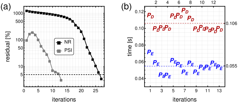
Figure 5: Truss example: (a) Evolution of the residual over iterations, Newton-Raphson solver (NR) v. phase-space iterative (PSI) solver (b) PSI time breakdown in each iteration: time invested in performing projection onto physically-admissible set ($P_{E}$) and onto materially-admissible set ($P_{D}$).

4.2.2 Solving without Euler-Lagrange equations: distance minimization

Instead of using the Euler-Lagrange equation, we could choose to minimize the distance directly during the $P_{D}$ step. This can be done in two ways: one in which a distance is specified based on a value of $\mathcal{C}$ for eq. 23, or another one in which the optimal value is always used, eq. 26.

The different performances can be seen in Figure 6: (a) shows the iterations leading to the solution when the optimal distance is used (13 iterations), while (b) evinces the slow convergence when $\mathcal{C}=0.1Y_{0}$ is used (112 iterations). So, ideally, one would use the optimal value $\mathcal{C}^{*}$ as this translates into an optimized distance function for each iteration, which seems to boost convergence (compare Figure 6(a) to (b)), even though the fitting of this “optimal-distance” approach into the context of projections into convex sets needs to be mathematically validated.

Table 7 reveals that the performance using the optimal distance does not dramatically change much when changing the method. Interestingly, cf. Table 4, the derivative-less method for solving this scalar minimization problem is faster than those that compute gradients and/or Hessians. On the contrary, the derivative-less method was slower when the phase-space was larger and thus the minimization required working with vectors, recall Section 3.4.

Table 7: Wallclock time comparisons using distance minimization for $P_{D}$ (different methods). Material defined by $p=2.0\cdot 10^{-4}$. Using $\mathcal{C}=\mathcal{C}^{*}$.

	Principal Axis (derivative-free)	Conjugate gradient	Quasi-Newton (BFGS)	Newton
Running time [s]	2.41	3.13	3.11	3.13

BFGS refers to Broyden–Fletcher–Goldfarb–Shanno method, a quasi-Newton method that does not require re-computing the Hessian [28].

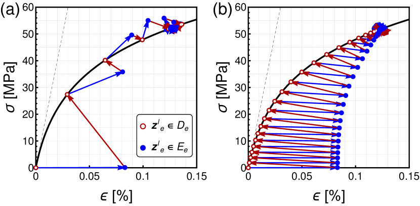
Figure 6: Iterations for one element, arrows represent successive projections. (a) Using distance minimization with optimal $\mathcal{C}$ and (b) using $\mathcal{C}=0.1Y_{0}$. First projection yields strain to satisfy essential BCs. The position of the physically-admissible set evolves as $E_{e}$ depends on $[\sigma_{e}]_{e=1}^{N_{e}}$, which change each time $P_{E}$ is applied at the structure level.

4.3 Influence of number of kenerls

Table 8: Wallclock time comparisons using distance minimization for $P_{D}$. Material defined by $p=10\cdot 10^{-4}$. Using $\mathcal{C}=\mathcal{C}^{*}$.

	Newton-Raphson solver	Phase-space iterative solver
		serial	2 kernels	4 kernels	8 kernels
Running time [s]	1.83	6.80	4.13	2.03	1.95

Similarly to the more complex phase space, Section 3.3, the scaling is good up to four processors. Afterward, Mathematica does not take advantage of the extra resources.

5 Discussion

Based on the examples analyzed above, there are three salient advantages in using PSI, all derived from the different treatment of the constitutive law: numerical handling of non-linearity, scalability, adaptability.

• Handling of non-linearity: since PSI does not update the stiffness matrix (nor its inverse), it avoids the poor-conditioning problem associated to local loss of stiffness in some elements [5, 3, 29].

• Scalability: whenever the $P_{D}$ projection is the performance bottleneck, we expect almost-linear time reduction when parallelizing this step and increasing the number of processors. Moreover, since this step is carried out on a per-element basis, the solver scales linearly with mesh size (number of elements).

• Adaptability: the two projections are but two minimizations. For the projection onto the physically-admissible set, enough continuity can be always assumed so that the corresponding Euler-Lagrange equations can be found, what yield a simple linear system in all cases. On the contrary, for non-linear constitutive laws, the per-element projection onto the materially-admissible set is intrinsically non-linear, so the user can opt among different ways of proceeding. Depending, on the dimensionality of the local phase space or the available libraries’ performance [30], one could choose among the multiple ways to carry out the projection onto the constitutive law.

The mathematical theory of alternating projections goes beyond the simple two-projection setting we have been using [31]. Some preliminary tests point to adding an intermediate third projection, consisting simply of evaluating the constitutive law, as a direct means to speed convergence up.

We also point out the possibility of splitting the system in two regions: one that remains linear-elastic and another one where inelastic behavior manifests. A classic linear-elastic solver for the former can be combined with phase-space iterations in the latter [32]; this could lead to even faster simulations of that kind of systems where non-linear material behavior is localized in space. Going one more step forward to an incremental-load scenario, we can envision localizing non-linearity both in space and time, where the parts of the domain that are solved in the traditional way or with phase-space iterations evolve dynamically with the load [33].

We also envision PSI solvers contributing to the adoption of neural-network based constitutive laws. In recent years, there has been a continuous stream [34, 35, 36, 37, 38] of excellent work that has proved the capacity of deep learning to represent complex, history-depedent, non-linear material behavior. However, the computation of gradients with respect to the value of the entries (strain components) via “automatic differentiation” [39] can be onerous and poorly-defined at times [40, 41, 42], e.g., since neural networks tend to feature activation functions with limited continuity [43] (for instance,“ReLu”). This logically hinders the teaming up of neural-network constitutive laws with Newton-Raphson solvers. Our new solver can work without ever having to compute derivatives of the constitutive law (see exercise in Section 3), thus avoiding the issue altogether. This renders the PSI solver as an ideal candidate to partner with this new generation of material constitutive models to pursue non-linear simulations, provided that the condition of the convexity of the convex law can be relaxed in some way.

6 Final remarks

We have introduced the concept of phase-space solvers, a new kind of iterative algorithm for solving problems in non-linear mechanics, and have shown its capacity to outperform traditional solvers when it comes to solve large systems with severe non-linearity. The method relies on projecting onto convex sets whose frontier is defined either by the material constitutive law or Newton’s second law. We have shown that, while the latter is achieved through solving a linear system of equations, the projection onto the constitutive law demands the element-wise resolution of either a non-linear optimization problem or a non-linear algebraic equation, but this step can be trivially parallelized, what renders the algorithm very efficient.

It remains to formally characterize errors [44] and convergence rates [45, 46, 47], but this seems a feasible task since much inspiration can be drawn from previous work on the method of alternating projections or the method of projections onto convex sets.

Logical future practical work avenues include dynamics [48] and finite kinematics [3, 4], apart from the aforementioned inelastic problems with complex loading paths.

Finally, we highlight that this approach can also be used to solve non-linear problems in other branches of physics, as long as they feature a constitutive law and some physical balance conditions (Newton’s second law, first law of thermodynamics…). As examples, let us mention heat transfer problems in complex media and flow of non-Newtonian fluids.

Appendix A Newton-Raphson (NR) method

As most iterative solvers, this procedure aims at minimizing the residual $r=\left\lVert\Delta F(\boldsymbol{u})\right\rVert=\left\lVert\boldsymbol{F}_{int}(\boldsymbol{u})-\boldsymbol{F}_{ext}\right\rVert$. This is done in incremental fashion, starting from some initial guess, e.g., $\boldsymbol{u}_{0}=\boldsymbol{0}$: assuming the solution at the $n$-th loading step is known ($\boldsymbol{u}_{n}$), then

$$\Delta\boldsymbol{u}_{n}=-\boldsymbol{T}(\boldsymbol{u}_{n})^{-1}\Delta\boldsymbol{F}_{n}=-\boldsymbol{T}(\boldsymbol{u}_{n})^{-1}\left[\boldsymbol{F}_{int}(\boldsymbol{u}_{n})-\boldsymbol{F}_{ext}\right]\,,$$ (28)

where $\boldsymbol{T}(\boldsymbol{u}_{n})$ is the tangent stiffness computed from the prior displacement field, and this $\boldsymbol{u}_{n+1}=\boldsymbol{u}_{n}+\Delta\boldsymbol{u}_{n}$. The tangent stiffness matrix is, in analytical form,

$$\boldsymbol{T}(\boldsymbol{u}_{n})={\partial\boldsymbol{F}\over\partial\boldsymbol{u}}\Big{|}_{\boldsymbol{u}=\boldsymbol{u}_{n}}\,,$$ (29)

which, in practice, must be re-assembled at every iteration and involves derivatives of the constitutive law, computed either analytically or numerically.

Oftentimes, for efficiency purposes, the new tangent stiffness is weighted with the one from prior steps or with the “undeformed” stiffness, i.e., $\boldsymbol{T}(\boldsymbol{u}_{n})\to\gamma\boldsymbol{T}(\boldsymbol{u}_{n})+(1-\gamma)\boldsymbol{T}(\boldsymbol{0})$.

For the sake of completeness, let us also mention the quasi-NR method, which computes the inverse tangent matrix only for the first iteration and then uses Sherman-Morrison formula to update this inverse, assuming rank-one matrices.

A word on the enforcement of Dirichlet BCs in the implementation of NR used in this work. We have opted for an approach that sets the known values directly on the initial guess, while subsequent iterations solved the incremental system eq. 28 only for the free dofs. This is a popular procedure, as its implementation is straighforward, but it can challenge the convergence of the method: having a strongly localized displacement field in the first guess around the nodes with essential BCs may lead to a deficient tangent stiffness matrix. This, in turn, may lead to nonsensical solutions or to difficulties when it comes to convergence. An antidote to this issue is precisely weighting tangent stiffness at every step with the zero-deformation stiffness matrix $\boldsymbol{T}(\boldsymbol{0})$.

References

- [1] K.J. Bathe. Finite Element Procedures. Prentice Hall, 2006.
- [2] E. Isaacson and H.B. Keller. Analysis of Numerical Methods. Dover Books on Mathematics. Dover Publications, 1994.
- [3] J.T. Oden. Finite Elements of Nonlinear Continua. Dover Civil and Mechanical Engineering. Dover Publications, 2013.
- [4] Olek C Zienkiewicz and Robert L Taylor. The finite element method. Vol. 2 : Solid and fluid mechanics, dynamics and non-linearity. McGraw-Hill, 4th ed. edition, 1991.
- [5] Robert D. Cook, David S. Malkus, Michael E. Plesha, and Robert J. Witt. Concepts and Applications of Finite Element Analysis, 4th Edition. Wiley, 4 edition, 2001.
- [6] Trenton Kirchdoerfer and Michael Ortiz. Data-driven computational mechanics. Computer Methods in Applied Mechanics and Engineering, 304:81–101, 2016.
- [7] John Von Neumann. On rings of operators. reduction theory. Annals of Mathematics, 50(2):401–485, 1949.
- [8] John Von Neumann. Functional operators: The geometry of orthogonal spaces, volume 2. Princeton University Press, 1951.
- [9] S. KACZMARZ. Approximate solution of systems of linear equations†. International Journal of Control, 57(6):1269–1271, 1993.
- [10] Jinchao Xu. Iterative methods by space decomposition and subspace correction. SIAM Review, 34(4):581–613, 1992.
- [11] Jinchao Xu and Ludmil Zikatanov. The method of alternating projections and the method of subspace corrections in hilbert space. Journal of the American Mathematical Society, 15(3):573–597, 2002.
- [12] Frank Deutsch. The Method of Alternating Orthogonal Projections, pages 105–121. Springer Netherlands, Dordrecht, 1992.
- [13] Lee C. Potter and K. S. Arun. A dual approach to linear inverse problems with convex constraints. SIAM Journal on Control and Optimization, 31(4):1080–1092, 1993.
- [14] D. Youla. Generalized image restoration by the method of alternating orthogonal projections. IEEE Transactions on Circuits and Systems, 25(9):694–702, 1978.
- [15] G. Demoment. Image reconstruction and restoration: overview of common estimation structures and problems. IEEE Transactions on Acoustics, Speech, and Signal Processing, 37(12):2024–2036, 1989.
- [16] Lyndon Clarke, Ian Glendinning, and Rolf Hempel. The mpi message passing interface standard. In Karsten M. Decker and René M. Rehmann, editors, Programming Environments for Massively Parallel Distributed Systems, pages 213–218, Basel, 1994. Birkhäuser Basel.
- [17] P. R. Amestoy, I. S. Duff, J. Koster, and J.-Y. L’Excellent. A fully asynchronous multifrontal solver using distributed dynamic scheduling. SIAM Journal on Matrix Analysis and Applications, 23(1):15–41, 2001.
- [18] P. R. Amestoy, A. Guermouche, J.-Y. L’Excellent, and S. Pralet. Hybrid scheduling for the parallel solution of linear systems. Parallel Computing, 32(2):136–156, 2006.
- [19] Charbel Farhat. A simple and efficient automatic fem domain decomposer. Computers & Structures, 28(5):579–602, 1988.
- [20] L. Hamandi, R. Lee, and F. Ozguner. Review of domain-decomposition methods for the implementation of fem on massively parallel computers. IEEE Antennas and Propagation Magazine, 37(1):93–98, 1995.
- [21] Edgar Gabriel, Graham E. Fagg, George Bosilca, Thara Angskun, Jack J. Dongarra, Jeffrey M. Squyres, Vishal Sahay, Prabhanjan Kambadur, Brian Barrett, Andrew Lumsdaine, Ralph H. Castain, David J. Daniel, Richard L. Graham, and Timothy S. Woodall. Open MPI: Goals, concept, and design of a next generation MPI implementation. In Proceedings, 11th European PVM/MPI Users’ Group Meeting, pages 97–104, Budapest, Hungary, September 2004.
- [22] François Broquedis, Jérôme Clet Ortega, Stéphanie Moreaud, Nathalie Furmento, Brice Goglin, Guillaume Mercier, Samuel Thibault, and Raymond Namyst. hwloc: a Generic Framework for Managing Hardware Affinities in HPC Applications. In IEEE, editor, PDP 2010 - The 18th Euromicro International Conference on Parallel, Distributed and Network-Based Computing, Pisa Italie, 02 2010.
- [23] Joshua Hursey, Ethan Mallove, Jeffrey M. Squyres, and Andrew Lumsdaine. An extensible framework for distributed testing of mpi implementations. In Proceedings, Euro PVM/MPI, Paris, France, October 2007.
- [24] Richard P Brent. Algorithms for minimization without derivatives. Courier Corporation, 2013.
- [25] Gianfranco Capriz. Continua with microstructure, volume 35. Springer Science & Business Media, 2013.
- [26] I.M. Gelfand and S.V. Fomin. Calculus of Variations. Raymond F. Boyer Library Collection. Prentice-Hall, 1963.
- [27] K. Karapiperis, M. Ortiz, and J.E. Andrade. Data-driven nonlocal mechanics: Discovering the internal length scales of materials. Computer Methods in Applied Mechanics and Engineering, 386:114039, 2021.
- [28] Dong C Liu and Jorge Nocedal. On the limited memory bfgs method for large scale optimization. Mathematical programming, 45(1-3):503–528, 1989.
- [29] Damage Mechanics, chapter 6, pages 67–218. John Wiley & Sons, Ltd, 2012.
- [30] Satish Balay, Shrirang Abhyankar, Mark F. Adams, Jed Brown, Peter Brune, Kris Buschelman, Lisandro Dalcin, Alp Dener, Victor Eijkhout, William D. Gropp, Dmitry Karpeyev, Dinesh Kaushik, Matthew G. Knepley, Dave A. May, Lois Curfman McInnes, Richard Tran Mills, Todd Munson, Karl Rupp, Patrick Sanan, Barry F. Smith, Stefano Zampini, Hong Zhang, and Hong Zhang. PETSc users manual. Technical Report ANL-95/11 - Revision 3.12, Argonne National Laboratory, 2019.
- [31] Eva Kopecká and Vladimír Müller. A product of three projections. Studia Math, 223(2):175–186, 2014.
- [32] Jie Yang, Wei Huang, Qun Huang, and Heng Hu. An investigation on the coupling of data-driven computing and model-driven computing. Computer Methods in Applied Mechanics and Engineering, 393:114798, 2022.
- [33] Sacha Wattel, Jean-François Molinari, Michael Ortiz, and Joaquin Garcia-Suarez. Mesh d-refinement: A data-based computational framework to account for complex material response. Mechanics of Materials, 180:104630, 2023.
- [34] M. Mozaffar, R. Bostanabad, W. Chen, K. Ehmann, J. Cao, and M. A. Bessa. Deep learning predicts path-dependent plasticity. Proceedings of the National Academy of Sciences, 116(52):26414–26420, 2019.
- [35] Filippo Masi, Ioannis Stefanou, Paolo Vannucci, and Victor Maffi-Berthier. Thermodynamics-based artificial neural networks for constitutive modeling. Journal of the Mechanics and Physics of Solids, 147:104277, 2021.
- [36] Filippo Masi and Ioannis Stefanou. Multiscale modeling of inelastic materials with thermodynamics-based artificial neural networks (tann). Computer Methods in Applied Mechanics and Engineering, 398:115190, 2022.
- [37] Xiaolong He and Jiun-Shyan Chen. Thermodynamically consistent machine-learned internal state variable approach for data-driven modeling of path-dependent materials. Computer Methods in Applied Mechanics and Engineering, 402:115348, 2022. A Special Issue in Honor of the Lifetime Achievements of J. Tinsley Oden.
- [38] Hernan J. Logarzo, German Capuano, and Julian J. Rimoli. Smart constitutive laws: Inelastic homogenization through machine learning. Computer Methods in Applied Mechanics and Engineering, 373:113482, 2021.
- [39] Mathieu Huot. Structural foundations for differentiable programming. PhD thesis, University of Oxford, 2022.
- [40] Thomas Beck and Herbert Fischer. The if-problem in automatic differentiation. Journal of Computational and Applied Mathematics, 50(1):119–131, 1994.
- [41] Wonyeol Lee, Hangyeol Yu, Xavier Rival, and Hongseok Yang. On correctness of automatic differentiation for non-differentiable functions. In H. Larochelle, M. Ranzato, R. Hadsell, M.F. Balcan, and H. Lin, editors, Advances in Neural Information Processing Systems, volume 33, pages 6719–6730. Curran Associates, Inc., 2020.
- [42] Wonyeol Lee, Sejun Park, and Alex Aiken. On the correctness of automatic differentiation for neural networks with machine-representable parameters, 2023.
- [43] Andrea Apicella, Francesco Donnarumma, Francesco Isgrò, and Roberto Prevete. A survey on modern trainable activation functions. Neural Networks, 138:14–32, 2021.
- [44] Selahattin Kayalar and Howard L Weinert. Error bounds for the method of alternating projections. Mathematics of Control, Signals and Systems, 1(1):43–59, 1988.
- [45] Heinz Bauschke, Frank Deutsch, Hein Hundal, and Sung-Ho Park. Accelerating the convergence of the method of alternating projections. Transactions of the American Mathematical Society, 355(9):3433–3461, 2003.
- [46] Catalin Badea, Sophie Grivaux, and Vladimir Müller. The rate of convergence in the method of alternating projections. St. Petersburg Mathematical Journal, 23(3):413–434, 2012.
- [47] Catalin Badea and David Seifert. Ritt operators and convergence in the method of alternating projections. Journal of Approximation Theory, 205:133–148, 2016.
- [48] Trenton Kirchdoerfer and Michael Ortiz. Data-driven computing in dynamics. International Journal for Numerical Methods in Engineering, 113(11):1697–1710, 2018.