Carrier Aggregation Enabled Integrated Sensing and Communication Signal Design and Processing
Abstract
The future mobile communication systems will support intelligent applications such as Internet of Vehicles (IoV) and Extended Reality (XR). Integrated Sensing and Communication (ISAC) is regarded as one of the key technologies satisfying the high data rate communication and highly accurate sensing for these intelligent applications in future mobile communication systems. With the explosive growth of wireless devices and services, the shortage of spectrum resources leads to the fragmentation of available frequency bands for ISAC systems, which degrades sensing performance. Facing the above challenges, this paper proposes a Carrier Aggregation (CA)-based ISAC signal aggregating high and low-frequency bands to improve the sensing performance, where the CA-based ISAC signal can use four different aggregated pilot structures for sensing. Then, an ISAC signal processing algorithm with Compressed Sensing (CS) is proposed and the Fast Iterative Shrinkage-Thresholding Algorithm (FISTA) is used to solve the reconfiguration convex optimization problem. Finally, the Cramér-Rao Lower Bounds (CRLBs) are derived for the CA-based ISAC signal. Simulation results show that CA efficiently improves the accuracy of range and velocity estimation.
Index Terms:
Carrier aggregation (CA), compressed sensing (CS), high and low-frequency band aggregation, high and low-frequency band cooperative sensing, integrated sensing and communication, Internet of vehicles (IoV), joint communication and sensing, multiple bands radar sensing, multiple bands radar OFDM pilots, signal design, signal processing.I Introduction
| Abbreviation | Description | Abbreviation | Description |
| 5G-A | 5th-Generation-Advanced | 6G | 6th-Generation |
| 2D | Two-dimensional | 3GPP | 3rd Generation Partnership Project |
| AWGN | Additive White Gaussian Noise | ADC | Analog-to-digital converter |
| BS | Base station | CRLB | Cramér-Rao Lower Bound |
| CCs | Component Carriers | CSI | Channel state information |
| CS | Compressed Sensing | CP | Cyclic Prefix |
| CA | Carrier aggregation | DFT | Discrete Fourier Transform |
| DAC | Digital-to-analog converter | FFT | Fast Fourier Transform |
| FISTA | Fast iterative shrinkage-thresholding algorithm | IDFT | Inverse Discrete Fourier Transform |
| IFFT | Inverse Fast Fourier Transform | ISAC | Integrated sensing and communication |
| IoV | Internet of Vehicle | IM | Index-modulation |
| ISI | Inter-symbol interference | LO | Local oscillator |
| mmWave | Millimeter wave | MAC | Media Access Control |
| OMP | Orthogonal Matching Pursuit | OFDM | Orthogonal Frequency Division Multiplexing |
| P/S | Parallel-to-serial conversion | RX | Receiver |
| RCS | Radar Cross Section | RIP | Restricted Isometry Property |
| RMSE | Root Mean Square Error | RCRLB | Root Cramér-Rao Lower Bound |
| S/P | Serial-to-parallel conversion | SNR | Signal-to-Noise Ratio |
| TX | Transmitter | XR | Extended Reality |
| Notation | Description | Notation | Description |
| Total number of subcarriers | Total number of OFDM symbols | ||
| Interval of comb pilot | Interval of block pilot | ||
| Total length of symbols in low-frequency | Total length of symbols in high-frequency | ||
| Subcarrier spacing in low-frequency | Subcarrier spacing in high-frequency | ||
| Carrier frequency in low-frequency | Carrier frequency in high-frequency | ||
| Length of CP | Channel information matrix in low-frequency | ||
| Channel information matrix in high-frequency | Range and velocity of target | ||
| Selection matrix | Complex conjugate of the complex number | ||
| Conjugate transpose, tanspose | Stacking matrix in columns | ||
| Hadamard product | Kronecker product |
The future 5th-Generation-Advanced (5G-A) and 6th-Generation (6G) mobile communication systems will support intelligent applications such as Internet of Vehicles (IoV) and Extended Reality (XR) [1]. These applications require both high data rate communication and highly accurate sensing. Designing a system with both communication and sensing functions is a promising solution to meet the above requirements [2]. With the rapid development of mobile communication systems, the frequency bands of communication systems are rising, which are getting close to the frequency bands of radar systems. Moreover, the signal processing methods and hardware structures of radar and communication systems are similar [3]. Hence, it is feasible to realize the integrated design of radar sensing and communication. The remarkable results of recent researches [3, 4, 5, 6] show that Integrated Sensing and Communication (ISAC) has the advantages of improving spectrum utilization and reducing device size, which is one of the promising key technologies in 5G-A and 6G.
Since the frequency bands of mobile communication systems are congested, the available spectrum resources for ISAC systems are fragmented, which will degrade the sensing performance. On one hand, there are deviations in sensing information such as Doppler frequency shifts carried by the echo signals in different frequency bands, making it difficult to directly apply multi-signal accumulation to improve the Signal-to-Noise Ratio (SNR) of the echo signals. On the other hand, when traditional radar sensing algorithms are applied to extract the sensing information from the echo signals on the fragmented spectrum resources, the fragmented spectrum will increase the level of sidelobe and decrease the sensing accuracy [7].
Hence, the efficient aggregation of the fragmented spectrum resources in radar sensing is a great challenge of ISAC signal processing on the congested frequency bands. In the field of communication, Carrier Aggregation (CA) techniques enable the aggregation of fragmented spectrum resources. CA is a spectrum expansion technique adopted by 3rd Generation Partnership Project (3GPP) to alleviate the shortage of contiguous resources. CA could be implemented in physical layer or Media Access Control (MAC) layer, which is divided into two categories, namely physical layer CA and MAC layer CA [8]. In physical layer CA, the selected Component Carriers (CCs) share a common transmission module, where the same modulation and coding techniques are applied. In MAC layer CA, the selected CCs use different transmission modules, where different modulation and coding techniques could be applied depending on the current Channel State Information (CSI) [9]. In terms of communication performance, according to the equation of channel capacity [10], CA significantly improves the channel capacity by increasing the bandwidth. According to [11, 12], in the field of ISAC signal design and processing, it is expected to introduce the idea of CA to aggregate fragmented spectrum resources to improve the resolution and accuracy of radar sensing.
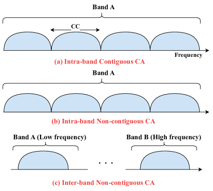
In general, there are three types of CA as shown in Fig. 1, namely intra-band contiguous CA, intra-band non-contiguous CA, and inter-band non-contiguous CA. The intra-band CA is equivalent to transmitting and receiving using larger points of Inverse Fast Fourier Transform (IFFT) and Fast Fourier Transform (FFT), so that the traditional Two-dimensional FFT (2D-FFT) algorithm is still applicable. Towards 5G-A, the sub-6 GHz and millimeter wave (mmWave) spectrum bands are standardized. Furthermore, the full-spectrum will be applied in 6G. Hence, the inter-band non-contiguous CA is widely applied since it realizes more efficient utilization of fragmented spectrum resources via aggregating high and low-frequency bands compared with the other two types of CA. Motivated by this observation, we adopt inter-band non-contiguous CA to aggregate the fragmented spectrum resources in ISAC signal design and processing. In addition, different types of CA correspond to different architectures of transmitter and receiver. In terms of inter-band CA, according to 3GPP TR 36.912 standard [13], a structure of multi-Radio Frequency (RF) chain is applied in this paper, as shown in Fig. 4. However, the different subcarrier spacing in high and low-frequency bands makes it difficult to directly fuse the sensing information in high and low-frequency bands to improve the sensing performance.
The researches on CA techniques applied to ISAC-enabled mobile communication systems are divided into two categories, namely the CA-enabled communication and the CA-enabled radar sensing. In terms of CA-enabled communication, Kang et al. [15] proposed a broadband high linearity drive amplifier that enables dual carrier aggregation and supports sub-GHz standards. Ginzberg et al. [16] proposed a digital linearisation scheme for a dual-channel discontinuous carrier aggregation transmitter which reduces the out-of-band distortion caused by CA. In terms of CA-enabled radar sensing, the radar signal processing for multi-band Orthogonal Frequency Division Multiplexing (OFDM) radar is the most related area. The stepped OFDM radar and frequency-agile stepped OFDM radar adopts the similar techniques in the intra-band non-contiguous CA. Clemens et al. [17] designed a stepped carrier OFDM signal, which combines 20 different frequency bands with 200 MHz bandwidth to form a 4 GHz bandwidth, achieving high range resolution. However, this signal processing method is only suitable for the targets with low mobility. Benedikt et al. [18] designed an improved Discrete Fourier Transform (DFT) algorithm that obtains high range and velocity resolution for automotive applications by offsetting the phase errors from the range. In [19], the concept of frequency-agile stepping OFDM is introduced to obtain high range resolution with limited bandwidth and gives a new Doppler processing. Furthermore, Knill et al. [20] presented a frequency-agile sparse OFDM radar signal processing method combined with Compressed Sensing (CS) technique to obtain the same sensing performance as equivalent OFDM signal on the continuous spectrum bands without increasing the sampling rate and bandwidth resources. However, the above studies do not involve the aggregation of high and low-frequency bands, where the differentiated subcarrier spacings bring a great challenge for the CA-enabled ISAC signal processing.
The other related research area of CA-based ISAC signal processing is multi-band radar, which improves the sensing accuracy over fragmented frequency bands by reconstructing the data in blank frequency bands. In 1974, Hogbom et al. [21] proposed a deconvolution-based method to estimate blank band data and construct a complete two-dimensional (2D) radar image. In 1992, Cuomo [22] introduced the linear predictive Band Width Extrapolation (BWE) technique using an autoregressive time series model to extrapolate bandwidth at blanking positions to achieve high range resolution. In 2004, Suwa et al. [23] proposed a Polarisation Band Width Extrapolation (PBWE) technique based on polarised radar data that achieves higher resolution than the conventional BWE technique. In 2009, Stoica et al. [24] applied the weighted least squares Iterative Adaptive Approach (IAA) in radar sensing and proposed a missing data recovery approach applicable to arbitrary data missing patterns. In 2015, Van Khanh et al. [25] applied the BWE technique to the Linear Frequency Modulation (LFM) narrow band radar and explored the BWE technique based on Matched Filtering (MF), which results in improved range resolution. In 2016, Zhang et al. [26] presented a coherent signal processing and multi-band fusion algorithm based on a sparse signal model, which is adaptable to the case of large spectral spacing between multi-band signals. However, the above studies are oriented for pulsed signal or LFM signal. The study on OFDM signal is very rare in the area of multi-band radar.
In this paper, we propose a CA-based staggered pilot structure for ISAC signal design. With CA techniques, the representative low and high-frequency bands, namely 5.9 GHz [27] and 24 GHz [28] frequency bands are selected as the fusion frequency bands. The parameters of OFDM signals are different in high and low-frequency bands, which brings challenge for the sensing information fusion in different frequency bands. Facing this challenge, the channel information matrix fusion method for CA-based staggered pilot ISAC signal is introduced. Then, a CS-based 2D-FFT algorithm is designed for ISAC signal processing. Finally, the Cramér-Rao Lower Bounds (CRLBs) for the proposed CA-based ISAC signal are derived. The detailed contributions are as follows.
-
CA-based staggered pilot ISAC signal: The staggered pilot structure is applied for CA-based ISAC signal design, where the block pilot is used in high-frequency band and the comb pilot is used in low-frequency band, which can comprehensively achieve better performance than other CA-based pilot signals.
-
Channel information matrix fusion method: With the proposed CA-based staggered pilot ISAC signal, the channel information matrix fusion method is proposed to fuse the sensing information in high and low-frequency bands with different parameters of OFDM signal such as subcarrier spacing and length of OFDM symbols.
-
CS-based 2D-FFT algorithm: The problem of sidelobe elevation and sensing performance degradation caused by the discontinuity of the modified channel information matrix is solved by the proposed CS-based 2D-FFT algorithm, which demonstrates strong anti-noise capability in target sensing.
-
CRLBs of CA-based ISAC Signal: The CRLBs for velocity and range estimation under the proposed ISAC signal are derived.
The rest of this paper is organized as follows. In Section II, the CA-based staggered pilot signal model is provided. In Section III, the ISAC signal processing methods are proposed. In Section IV, the CRLBs for range and velocity estimation are revealed. In Section V, simulation results are presented. Finally, this paper is summarized in Section VI. Table I shows the abbreviations and notations used in this paper.
II Carrier Aggregation-based ISAC Signal
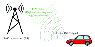
As shown in Fig. 2, the ISAC system for vehicle communication and sensing is considered. The OFDM signals on 5.9 GHz and 24 GHz frequency bands are representative frequency bands for vehicular communication [29]. Hence, this paper adopts 5.9 GHz and 24 GHz frequency bands to design the CA-based ISAC signal. To make full use of spectrum resources and achieve highly accurate sensing performance, the CA-based staggered pilot ISAC signal is designed.
II-A The CA-based staggered pilot ISAC signal
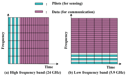
As shown in Fig. 3, the structure of the CA-based staggered pilot ISAC signal is provided. Fig. 3(a) represents the structure of block pilot in high-frequency band, which is discrete in time domain and continuous in frequency domain, so that the signal is insensitive to frequency-selective fading. Fig. 3(b) shows the structure of comb pilot in low-frequency band, which is discrete in frequency domain and continuous in time domain. Therefore, the signal is insensitive to time-selective fading.
The comb pilot signal in low-frequency band at the transmitter (TX) is expressed as [30]
| (1) |
where is the number of subcarriers at the comb pilot location in each OFDM symbol, is the total number of subcarriers in each OFDM symbol, and is the interval of comb pilot. It is noted that is a pre-requisite for the range estimation, where and are the subcarrier spacings in low and high-frequency bands, respectively. Similarly, the time-domain expression of the block pilot signal in the high-frequency band is [31]
| (2) |
where is the number of OFDM symbols at the block pilot location in a frame, is the total number of OFDM symbols transmitted in one frame of data, and is the interval of block pilot. According to (1) and (2), the CA-based staggered pilot ISAC signal is expressed as
| (3) | ||||
where and denote the modulation symbols in low and high-frequency bands, respectively. and represent the carrier frequencies of the low and high-frequency bands, respectively.
The echo signal reflected from the target contains Doppler frequency shift and delay , where and are the range and relative velocity of target, respectively, and is the wavelength of signal. Therefore, the echo signal at the receiver (RX) after down-conversion is expressed as
| (4) | ||||
where and are the channel gain on the -th subcarrier of the -th OFDM symbol at high and low-frequency bands, respectively, which consist of channel fading and Radar Cross Section (RCS), is the Additive White Gaussian Noise (AWGN). and represent the total length of the OFDM symbols in low and high-frequency bands, respectively. The symbol length is , with representing the length of Cyclic Prefix (CP) and representing the subcarrier spacing.
In addition to the above CA-based staggered pilot signal, there are other three aggregated structured signals, which are high-frequency comb and low-frequency block aggregated pilot signal in (5), high and low-frequency full-block aggregated pilot signal in (6), and high and low-frequency full-comb aggregated pilot signal in (7), where the interval of comb pilot is , and the interval of block pilot is .
| (5) | ||||
| (6) | ||||
| (7) | ||||
II-B Framework of ISAC signal processing
II-B1 Signal processing at TX
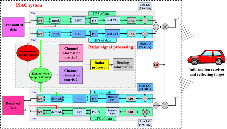
As shown in Fig. 4, the transmitted data is divided into two data streams: High-frequency Stream (HFS) and Low-frequency Stream (LFS), which are also denoted by high-frequency CC and low-frequency CC, respectively. In the HFS, the transmitted data is modulated to form a modulated symbol. Undergoing block-wise inverse fast Fourier transform, subsequent parallel-to-serial conversion and the addition of CP, the signal is converted to an analog signal and mixed with the high-frequency LO signal to provide a high-frequency analog signal [32]. Compared with the HFS, the LFS is mixed with the low-frequency LO to obtain low-frequency analog signal. Then, the low-frequency analog signal and high-frequency analog signal are combined and fed into a single antenna [13]. When the multiple antennas are applied, we need to consider precoding schemes to improve the performance of communication and sensing. Since a single antenna is applied in this paper, the problems associated with multiple antennas are not considered.
II-B2 Signal processing at RX
For communication, the demodulation process is similar to traditional OFDM demodulation [33] since the data stream has been separated into HFS and LFS at RX. At the RX, the same steps are performed in reverse order. The received modulated symbol is recovered by FFT. Then, we can also use the traditional maximum likelihood detection to obtain the communication data. For sensing, the modulated symbols at RX are divided by the modulated symbols at TX to obtain the channel information matrix, which is used for radar sensing. A detailed description of the ISAC signal processing is provided in Section III.
The differences in the subcarrier spacings and the length of OFDM symbols in high and low-frequency bands bring challenges for the processing of the CA-based ISAC signal processing, which will be solved in Section III.
III ISAC Signal Processing
In terms of radar signal processing for OFDM-based ISAC signal, Sturm et al. [32] proposed 2D-FFT algorithm, which takes full advantage of the 2D structure of OFDM signal in efficient radar sensing [1]. Zuo et al. [34] proposed a CS-based radar signal processing for index-modulated OFDM (OFDM-IM) signals. Based on these previous approaches, we propose a CA-based ISAC signal processing algorithm in this section.
The CS methods apply the sparsity of echo signal to reconstruct the incompletely sampled channel information matrix in 2D-FFT method, thus reducing the Fourier sidelobe deterioration. The channel information matrix is expressed as
| (8) |
where X represents range-velocity profile of target, and are Fourier transform matrices, respectively. is the total number of subcarriers, is the number of OFDM symbols, is the conjugate transpose of the matrix, is AWGN matrix. The selection matrix is defined to filter out valid data based on subcarrier activation. The filtering process is shown in Fig. 5. Multiplying both sides of (8) by the matrix J, we have
| (9) |
where
| (10) |
In (10), represents stacking matrix in columns, refers to Kronecker product, A is the sensing matrix in CS. When x is a sparse vector and A satisfies the Restricted Isometry Property (RIP) condition [35], the sparse signals can be reconstructed. Since the solution of (9) is NP-hard, (9) is transformed into (11).
| (11) |
Problem (11) is a least square optimization problem that can be solved by the Orthogonal Matching Pursuit (OMP) algorithm. OMP is an iterative greedy algorithm that is utilized to recover high-dimensional sparse signals from a limited number of noisy linear measurements. During each iteration, OMP selects the column that exhibits the highest correlation with the current residual and incorporates it into the set of chosen columns. Detailed descriptions of OMP can be found in [36]. By solving (11), the range-velocity profile is obtained for the complete OFDM signal, avoiding the effect of Fourier sidelobe deterioration.
In this section, the CA-based ISAC signal processing algorithm is proposed, which takes full advantage of the two channel information matrices in high and low-frequency bands, resulting in better sensing performance.
The CA-based staggered pilots signal adopts comb pilot in low-frequency band with interval of and block pilot in high-frequency band with interval of . According to Fig. 4, when the low-frequency and high-frequency data streams pass through the DAC, they are mixed with high and low-frequency LOs to obtain high and low-frequency analog signals. At RX, the mixed high and low-frequency analog signals are separated by matched filtering. Using element-wise complex division, the channel information matrix in low-frequency band and the channel information matrix in high-frequency band are obtained at the RX.
| (12) | ||||
where denotes Hadamard product. Combining the structures of high-frequency block pilot and low-frequency comb pilot, we have
| (13) | ||||
where . And we have
| (14) | ||||
where . In order to represent the structural form of the two channel information matrices clearly, the matrices are rewritten as (15) and (16), where the elements in and denote the elements after the division of the received modulation symbols by the transmitted modulation symbols.
| (15) |
| (16) |
III-A Range Estimation Method
The different subcarrier spacings in high and low-frequency bands bring challenges for the range estimation using CA-based ISAC signal. According to 2D-FFT algorithm, the column vector of channel information matrix is applied in calculating the range of target [32].
III-A1 Fusion of channel information matrices
Comparing (13) and (14), it is discovered that the different parameters between and are and . As mentioned in Section II, . Replacing the variable in with , the transformation of is
| (17) |
where is the interval of comb pilot. Comparing in (17) and in (14), is a subsequence of the preceding elements of .
III-A2 CS-based range estimation algorithm
In order to estimate the range of target, the modulation symbols in high and low-frequency bands at the RX are recovered. Then, the channel information matrix in high-frequency band and the channel information matrix in low-frequency band are obtained. The elements of in the positions of pilot’s subcarriers are rearranged, and the channel information matrix is obtained. Finally, in order to overcome the impact of non-continuous subcarriers or symbols on the performance of sensing, the CS-based target estimation method in [34] is applied, which has been introduced at the beginning of Section III. The sensing matrix in [34] needs to be adjusted for non-continuous situations. The process of adjusting the sensing matrices used in this paper is described below. Beck et al. proposed the fast iterative shrinkage-thresholding algorithm (FISTA) [37], which applies the gradient descent to solve optimization problems. FISTA achieves fast convergence by generalizing the iterative idea of Nesterov’s method [38]. Thus, FISTA is used instead of the OMP reconstruction algorithm to obtain fast convergence speed. The above algorithm is referred to as CS-IDFT. When processing the channel information matrix , a column in the channel information matrix is selected to obtain the sensing matrix based on the location of the valid data in a column. Define a selection matrix as follows, where the elements in the first rows are and the rest elements are .
| (18) |
The sensing matrix in CS is represented as the product of the sparse basis and the measurement matrix. The channel information matrix can be transformed to the range-Doppler domain under the discrete Fourier transform basis, while the radar signals are generally sparse in the range-velocity domain [20]. Therefore, the sensing matrix in this paper takes the form of Fourier transform basis. is the discrete inverse Fourier matrix. Hence, the modified sensing matrix is . For the remaining columns, the sensing matrix is obtained as (18). Using the sensing matrix and the data in each column of , we can obtain power spectrum of range by solving (11). The range estimation algorithm is shown in Algorithm 1, which is explained intuitively in Fig. 6. The channel information matrix in low-frequency band is firstly processed to obtain the rearranged matrix . Then, the power spectrum of range is obtained using the CS-IDFT algorithm for . The power spectrum of range is obtained using the IDFT of the channel information matrix in high-frequency band. The power spectra of range in high and low-frequency bands are superimposed. Finally, the index value is obtained by searching the peak of the superimposed power spectrum and the estimated range of target is
| (19) |
| Algorithm 1: Range Estimation Algorithm | |||||||||
| Input: |
|
||||||||
| 1: | For the row vector of in steps do | ||||||||
| 2: | Initialize a zero matrix and ; | ||||||||
| 3: | Deposit the row of into -th row of ; | ||||||||
| 4: | ; | ||||||||
| 5: | End For | ||||||||
| 6: | Initialize a power spectrum of range and ; | ||||||||
| 7: | For the column vector of in steps do | ||||||||
| 8: |
|
||||||||
| 9: | ; | ||||||||
| 10: | End For | ||||||||
| 11: | For each column vector of do | ||||||||
| 12: |
|
||||||||
| 13: | The result of output of the FISTA is assigned to ; | ||||||||
| 14: | ; | ||||||||
| 15: | End For | ||||||||
| 16: | Normalize and perform a peak search on it; | ||||||||
| 17: |
|
||||||||
| Output: | The estimation of the range | ||||||||
III-B Velocity Estimation Method
In the estimation of target’s velocity, the difference in carrier frequencies in high and low-frequency bands leads to different resolutions of the velocity estimation, which brings challenges for the fusion of sensing information in high and low-frequency bands.
III-B1 Fusion of channel information matrices
The relative velocity of target introduces a linear phase shift along the time axis, so that only the row vectors of channel information matrix need to be considered.
By observing in (13) and in (14), it is discovered that the different parameters are , and . As revealed in Fig. 4, the data streams of HFS and LFS use different modules of adding CP, which can dynamically adjust CP length. On the premise of meeting the maximum ranging, can be satisfied by adding CP with different lengths. According to 2D-FFT method [32], is obtained. Therefore, when the FFT is performed on the row vectors of high and low-frequency channel information matrices, the peak index values will be the same with . Therefore, the velocity of target can be estimated by the accumulation of high and low-frequency channel information matrices.
III-B2 CS-based velocity estimation algorithm
By observing in (14), it is revealed that the row vector contains the null modulation symbol, and Fourier transform will cause the increase of sidelobe. According to [7], sidelobe and noise can be reduced by the estimation method based on CS. The FISTA reconstruction algorithm is used instead of the OMP algorithm. The algorithm here is refered to CS-DFT. When processing the channel information matrix , the sensing matrix for the first row vector in is obtained based on the location of the valid data in the first row of . A selection matrix is defined based on the interval of block pilot and the number of OFDM symbols
| (20) |
where each column of P is
| (21) |
Then the sensing matrix is obtained. For the remaining rows, the sensing matrix is obtained as (20). Using the sensing matrix and the data in each row of , the power spectrum of velocity is obtained by solving (11). The velocity estimation algorithm is shown in Algorithm 2, which is explained intuitively in Fig. 7. The power spectrum of velocity is obtained by using the CS-DFT algorithm for the high-frequency channel information matrix. Then, the DFT is performed on the low-frequency channel information matrix according to the pilot position to obtain the power spectrum of velocity. The power spectra of velocity in high and low-frequency bands are superimposed. Finally, the index value is obtained by searching the peak of the superimposed power spectrum and the estimated velocity of target is
| (22) |
| Algorithm 2: Velocity Estimation Algorithm | |||||||||
| Input: |
|
||||||||
| 1: | Initialize a power spectrum of velocity and ; | ||||||||
| 2: | For the -th row vector of in steps do | ||||||||
| 3: |
|
||||||||
| 4: | ; | ||||||||
| 5: | End For | ||||||||
| 6: | For each row vector of do | ||||||||
| 7: |
|
||||||||
| 8: | The result of output of the FISTA is assigned to ; | ||||||||
| 9: | ; | ||||||||
| 10: | End For | ||||||||
| 11: | Normalize and perform a peak search on it; | ||||||||
| 12: |
|
||||||||
| Output: | The estimation of the range | ||||||||
IV Performance of CA-based ISAC Signal
In this section, the sensing performance of CA-based ISAC signals is analyzed using Root Mean Square Error (RMSE) and CRLB. Firstly, the ISAC signal processing algorithms under different pilot structures are provided. Then, the CRLBs of ISAC signals under different pilot structures are derived.
IV-A Other Types of Pilot Structures
The above CA-enabled ISAC signal design adopts the pilot structure with block pilot in high-frequency band and comb pilot in low-frequency band. However, there are three other pilot structures, which are high-frequency comb and low-frequency block aggregated pilot, high and low-frequency full-block aggregated pilot, and high and low-frequency full-comb aggregated pilot. The signal processing procedures under the other three pilot structures are as follows.
IV-A1 High-frequency comb and low-frequency block aggregrated pilot
The steps of signal processing are as follows.
-
•
Step 1: The low-frequency channel information matrix and the high-frequency channel information matrix are obtained.
-
•
Step 2: We perform IDFT on the column vectors corresponding to the block pilot positions of , sum the results, search the power spectrum for the peak index value, and combine it with (19) to get the range estimate . Likewise, we perform CS-DFT on every row vector of , sum the results, combine the peak index value with (22) to get the velocity estimation .
-
•
Step 3: We perform CS-IDFT on every column vector of , sum the results, search the power spectrum for the peak index value, and combine it with (19) to get the range estimation . Likewise, we perform DFT on the row vectors corresponding to the comb pilot positions of , sum the results, combine the peak index value with (22) to get the velocity estimation .
-
•
Step 4: We take the average of and , and the average of and to get the final estimation.
IV-A2 High and low-frequency full-block aggregated pilot
The steps of signal processing are as follows.
-
•
Step 1: The low-frequency channel information matrix and the high-frequency channel information matrix are obtained.
-
•
Step 2: Since both channel information metrics are block-pilot structures, only the processing of is provided here and the processing of is consistent. We perform IDFT on the column vectors corresponding to the block pilot positions of , sum the results, search the power spectrum for the peak index value, and combine it with (19) to get the range estimation . Likewise, we perform CS-DFT on every row vector of , sum the results, combine the peak index value with (22) to get the velocity estimation . Then, the same process is performed on to get and .
-
•
Step 3: We take the average of and , and the average of and to get the final estimation.
IV-A3 High and low-frequency full-comb aggregated pilot
The steps of signal processing are as follows.
-
•
Step 1: The low-frequency channel information matrix and the high-frequency channel information matrix are obtained.
-
•
Step 2: Since both channel information metrics are comb-pilot structures, only the processing of is provided here, and the processing of is consistent. We perform CS-IDFT on every column vector of , sum the results, search the power spectrum for the peak index value, and combine it with (19) to get the range estimation . Likewise, we perform DFT on the row vectors corresponding to the comb pilot positions of , sum the results, combine the peak index value with (22) to get the velocity estimation . Then, the same process is performed on to get and .
-
•
Step 3: We take the average of and , and the average of and to get the final estimation.
To verify the superiority of the staggered pilot structure chosen in this paper, the RMSE performance of various pilot structures is compared in Section V.
IV-B CRLBs of Various Pilot Structures
The CRLBs of CA-enabled ISAC signals under different pilot structures are derived. It is noted that since the carrier frequencies in high and low-frequency bands are different and the estimator of Doppler frequency shift contains the carrier frequency . To facilitate theoretical derivation, we take out the carrier frequency and set the estimator as . In this way, when performing the derivation, we do not have to pay attention to the effect of the different carrier frequencies in high and low-frequency bands. The received echo signal at RX can be expressed as
| (23) |
where denotes the product of the channel attenuation factor and the amplitude of transmitted signal, is the AWGN, represents the index of -th symbol, and represents the index of -th subcarrier. It is revealed that and are unknown in the received echo signal, which contain the range and velocity information of target. Therefore, joint estimation of parameters and is required. The log-likelihood function is
| (24) | ||||
where denotes the complex conjugate of the complex number and
| (25) | ||||
| (26) |
The first derivative of and can be expressed as
| (27) | ||||
| (28) | ||||
The second derivative of is
| (29) | ||||
Upon taking the negative expectation of (29), we have
| (30) | ||||
Similarly, the negative expectation of the second derivative of can be obtained
| (31) | ||||
| (32) | ||||
Then, the Fisher information matrix can be derived as
| (33) | ||||
and
| (34) | ||||
| (35) | ||||
According to the transformation relation of and , the CRLBs of range and velocity estimation are
| (36) |
| (37) |
IV-B1 CRLB of CA-based staggered pilot signal
According to Section III, the interval of comb pilot satisfies , so that we have in the derivation of CRLB. According to (34) and (36), the CRLB of range estimation is
| (38) | ||||
Then, combining with the process of Algorithm 1, the sum in (38) is the sum of two channel information matrices in high and low-frequency bands. Therefore,
| (39) | ||||
| (40) | ||||
| (41) | ||||
where is the number of subcarriers occupied by the pilot in low-frequency band, is the number of OFDM symbols occupied by the pilot in high-frequency band. By substituting (39), (40), and (41) into (38), the CRLB of range estimation of CA-based staggered pilot signal is (42).
| (42) |
| (43) |
In terms of velocity estimation, is known using Algorithm 2, so that only one pair of parameters, namely and , are selected when deriving CRLB. Firstly, (44) can be obtained according to (35) and (37).
| (44) | ||||
Then, according to Algorithm 2, the sum in (44) is the sum of two channel information matrices in high and low-frequency bands. Similarly, substituting (39), (40), and (41) into (44), the CRLB of velocity estimation of the CA-based staggered pilot ISAC signal is shown in (43).
| (45) |
| (46) |
The CRLBs for the CA-enabled ISAC signals under the remaining pilot structures are provided as follows. For the simplicity in deriving the CRLBs, the comb pilot intervals of low and high-frequency bands are set the same, which is denoted by . Meanwhile, the block pilot intervals of low and high-frequency bands are set the same, denoting by .
IV-B2 CRLB with high-frequency comb and low-frequency block aggregated pilot
IV-B3 CRLB with high and low-frequency full-block aggregated pilot
IV-B4 CRLB with high and low-frequency full-comb aggregated pilot
| (47) |
| (48) |
| (49) |
| (50) |
V Simulation Results and Analysis
| Symbol | Parameter | Low frequency | High frequency |
| Carrier frequency | 5.9 GHz | 24 GHz | |
| Number of OFDM symbols | 64 | 64 | |
| Number of subcarriers | 512 | 512 | |
| Comb pilot interval | 4 | 4 | |
| Block pilot interval | 4 | 4 | |
| Subcarrier spacing | 30 kHz | 120 kHz | |
| Total OFDM symbol duration | 39.5 s | 9.7 s | |
| Bandwidth of signal | 15.4 MHz | 61.4 MHz |
In this section, the power spectrum and RMSE of radar sensing are simulated to verify the feasibility and performance of the proposed CA-based ISAC signal design and processing methods. Then, the RMSEs and CRLBs of the four pilot structures are simulated.
Firstly, we assume that the maximum unambiguous velocity of sensing is m/s. The subcarrier spacing in the 5.9 GHz low-frequency band is 30 kHz, while the subcarrier spacing in the 24 GHz high-frequency band is 120 kHz according to the 3GPP TS 38.211 standard [40] and subcarrier spacing design principle in [39]. With the farthest detection distance 200 m, the length of CP must be greater than the maximum multipath delay spread, so that the length of CP must be greater than 1.33 s and there is no inter-symbol interference (ISI). The parameters in simulation are summarized in Table II, which satisfies the scenario of vehicle communication and sensing.
V-A Performance of Radar Sensing
In this subsection, the feasibility and sensing performance of the proposed ISAC signal processing algorithm are verified by simulating the power spectrum and RMSE of radar sensing according to the parameters in Table II. The power spectra for range and velocity estimation are simulated with the range of target 117 m, the relative velocity of target 30 m/s and the SNR 10 dB, as shown in Fig. 8 and Fig. 9, respectively. X and Y in the figure are used to indicate the peak and the corresponding index value. As the power spectrum is normalized, so that it corresponds to the peak position when . According to the indexes of the peaks of the power spectra, the target’s range and velocity are estimated as follows.
| (51) |
| (52) |
where and represent the peak index value of the power spectra of range and velocity, respectively.
It is revealed that the error of range estimation is 0.1875 m and the error of velocity estimation is 0.3176 m/s. Then, RMSE is used to reveal the deviation between the estimated value and the real value. The performance of range and velocity estimation using high-frequency signal is better than that using low-frequency signal. Meanwhile, the block pilot signal performs better in range estimation and the comb pilot siganl performs better in velocity estimation. Hence, the CA-based staggered pilot signal is compared with high-frequency block pilot signal in range estimation and is compared with high-frequency comb pilot signal in velocity estimation to verify the performance improvement using CA.
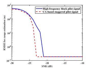
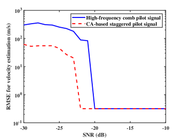
The RMSE of the high-frequency signal and the CA-based staggered pilot signal for range and velocity estimation are shown in Fig. 10 and Fig. 11, respectively. It is revealed that the RMSEs of the range and velocity estimation with the proposed ISAC signal, namely the CA-based staggered pilot signal, are smaller than those with high-frequency block pilot signal and high-frequency comb pilot signal, respectively. Hence, the CA-based staggered pilot signal has better anti-noise capability and sensing performance than the signals without CA.
V-B CRLB of Range and Velocity Estimation
The CRLBs of CA-based staggered pilot ISAC signals is simulated. Then, the comparison of Root CRLBs (abbreviated as RCRLBs) and RMSE is simulated based on the parameters in Table II.
V-B1 CRLB analysis
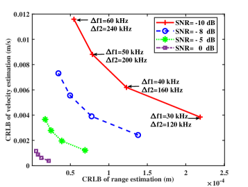
As shown in Fig. 12, when the SNR is fixed, the CRLB of range estimation is decreasing with the increase of the CRLB of velocity estimation, namely, the CRLBs of range and velocity estimation have a tradeoff relation. The reason is that the CRLB of velocity estimation is proportional to the subcarrier spacing, whereas the CRLB of range estimation is inversely proportional to the subcarrier spacing. Besides, when the subcarrier spacing is fixed, the CRLBs of range and velocity estimation are decreasing with the increase of SNR.
V-B2 CRLB comparison
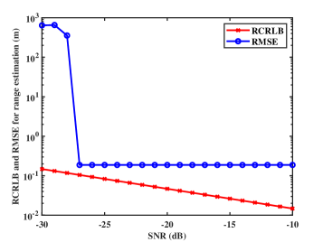
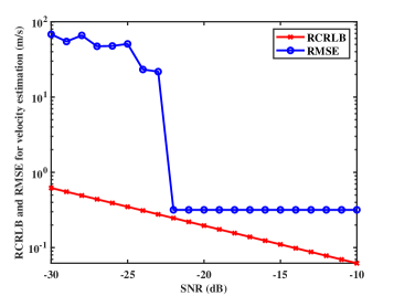
Fig. 13 and Fig. 14 show the comparison of RCRLB and RMSE for range and velocity estimation, respectively. It is observed that the RCRLB is smaller than the RMSE because the RCRLB reveals the lower bound of the minimum root variance of unbiased estimation. Meanwhile, the 2D-FFT algorithm has a fixed resolution due to the fixed sampling rate and number of FFT points in the simulation, causing the RMSE to converge to a fixed value in the high SNR regime.
V-C Simulation Comparison of Four Pilot Structures
In this subsection, we simulate the RMSEs and CRLBs for four pilot structures based on the parameters in Table II.
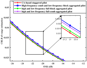
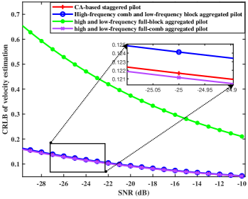
V-C1 CRLBs of four pilot structures
According to (42) - (50), the CRLBs for range and velocity estimation with the four pilot structures are shown in Fig. 15 and Fig. 16, respectively. As revealed in Fig. 15, the CA-based staggered pilot has the lowest CRLB. Therefore, when the ISAC-enabled mobile communication system is mainly used to obtain high-accurate range estimation of target, the CA-based staggered pilot structure is the optimal choice. In terms of velocity estimation, as shown in Fig. 16, the high and low-frequency full-comb aggregated pilot has the lowest CRLB, followed by the CA-based staggered pilot. It is observed that the gap of the CRLBs between the low-frequency full-comb aggregated pilot and the CA-based staggered pilot is small. Therefore, when the ISAC-enabled mobile communication system is mainly used to obtain high-accurate velocity estimation of target, both the high and low-frequency full-comb aggregated pilot and the CA-based staggered pilot structure can be chosen.
CRLB comparisons are performed theoretically. In practice, the sensing performance of various pilot structures depends on the signal processing algorithms. Therefore, in the following, we simulate the RMSE of four pilot structures using the algorithm proposed in this paper.
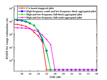
V-C2 RMSEs of four pilot structures
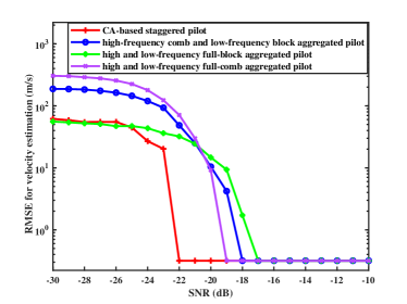
The RMSEs for range and velocity estimation with the four pilot structures are shown in Fig. 17 and Fig. 18, respectively. As revealed in Fig. 17, the CA-based staggered pilot has the fastest convergence speed among the four pilot structures. When the SNR is large than the threshold -22 dB, the RMSE of range estimation with the CA-based staggered pilot remains constant. While the thresholds of SNR with other pilot structures are smaller than -22 dB. Hence, in terms of range estimation, the CA-based staggered pilot has the best performance among the four pilot structures.
In terms of velocity estimation, as shown in Fig. 18, the CA-based staggered pilot has the fastest convergence speed among the four pilot structures. When the SNR is larger than the threshold -22 dB, the RMSE of velocity estimation with CA-based staggered pilot is converged to a constant value. While the thresholds of SNR with other pilot structures are smaller than -22 dB. Therefore, the CA-based staggered pilot has the best velocity estimation performance among the four pilot structures.
VI Conclusion
This paper proposes the CA-based ISAC signals to improve sensing performance by aggregating discontinuous high and low-frequency bands. Then, the radar signal processing algorithms based on 2D-FFT and CS are proposed, which fuse the sensing information from high and low-frequency bands. The CRLBs of range and velocity estimation with the proposed ISAC signals are analyzed. The feasibility and performance improvement of the ISAC signals proposed in this paper are verified by simulation results. It is revealed that the CA-based ISAC signal has better sensing performance compared with the ISAC signal without CA. Since the full spectrum is one of the promising key technologies in 6G, which efficiently aggregates the low and high-frequency bands to provide high communication data rate, the CA-enabled ISAC signals proposed in this paper may provide a guideline for the ISAC system design in the era of 6G. The future research problems focus on the sensing algorithms with different path losses on high and low frequency bands and the effect of nonlinear high-frequency power amplifier of transmitter RF.
References
- [1] Z. Wei, H. Qu, Y. Wang, X. Yuan, H. Wu, Y. Du, K. Han, N. Zhang, and Z. Feng, “Integrated Sensing and Communication Signals Towards 5G-A and 6G: A Survey,” IEEE Internet of Things Journal, Jan 2023.
- [2] P. Kumari, J. Choi, N. González-Prelcic, and R. W. Heath, “IEEE 802.11 ad-Based Radar: An Approach to Joint Vehicular Communication-Radar System,” IEEE Transactions on Vehicular Technology, vol. 67, no. 4, pp. 3012–3027, Nov 2017.
- [3] Z. Feng, Z. Fang, Z. Wei, X. Chen, Z. Quan, and D. Ji, “Joint radar and communication: A survey,” China Communications, vol. 17, no. 1, pp. 1–27, Jan 2020.
- [4] Z. Wang, K. Han, J. Jiang, Z. Wei, G. Zhu, Z. Feng, J. Lu, and C. Meng, “Symbiotic Sensing and Communications Towards 6G: Vision, Applications, and Technology Trends,” in 2021 IEEE 94th Vehicular Technology Conference (VTC2021-Fall). IEEE, Dec 2021, pp. 1–5.
- [5] S. Li, W. Yuan, C. Liu, Z. Wei, J. Yuan, B. Bai, and D. W. K. Ng, “A Novel ISAC Transmission Framework Based on Spatially-Spread Orthogonal Time Frequency Space Modulation,” IEEE Journal on Selected Areas in Communications, vol. 40, no. 6, pp. 1854–1872, Mar 2022.
- [6] W. Yuan, Z. Wei, S. Li, J. Yuan, and D. W. K. Ng, “Integrated Sensing and Communication-Assisted Orthogonal Time Frequency Space Transmission for Vehicular Networks,” IEEE Journal of Selected Topics in Signal Processing, vol. 15, no. 6, pp. 1515–1528, Oct 2021.
- [7] G. Huang, “Research on Modulation Techniques for Fusion of Radar and Communications,” Ph.D. dissertation, Guilin University Of Electronic Technology, Jun 2021.
- [8] Carrier Aggregation explained. [Online]. Available: {https://www.3gpp.org/technologies/101-carrier-aggregation-explained}
- [9] R. Ratasuk, D. Tolli, and A. Ghosh, “Carrier Aggregation in LTE-Advanced,” in 2010 IEEE 71st Vehicular Technology Conference. IEEE, Jun 2010, pp. 1–5.
- [10] A. Goldsmith, Wireless communications. Cambridge university press, 2005.
- [11] R. Thomä, T. Dallmann, S. Jovanoska, P. Knott, and A. Schmeink, “Joint communication and radar sensing: An overview,” in 2021 15th European Conference on Antennas and Propagation (EuCAP). IEEE, Mar 2021, pp. 1–5.
- [12] T. Wild, V. Braun, and H. Viswanathan, “Joint design of communication and sensing for beyond 5G and 6G systems,” IEEE Access, vol. 9, pp. 30 845–30 857, Feb 2021.
- [13] 3GPP, “Feasibility Study for Further Enhancements for E-UTRA (LTE Advanced) (Release 9),” 3rd Generation Partnership Project (3GPP), Technical Report (TR) 36.912, Sep 2009.
- [14] H. Lee, S. Vahid, and K. Moessner, “A Survey of Radio Resource Management for Spectrum Aggregation in LTE-Advanced,” IEEE Communications Surveys & Tutorials, vol. 16, no. 2, pp. 745–760, Nov 2013.
- [15] D.-W. Kang and J.-H. Choi, “A dual-path high linear amplifier for carrier aggregation,” ETRI Journal, vol. 42, no. 5, pp. 773–780, Oct 2020.
- [16] N. Ginzberg, T. Gidoni, and E. Cohen, “Carrier Aggregation Transmitter Linearization using 2D-DPD and Out-of-Band IM3 Cancellation,” in 2022 IEEE Topical Conference on RF/Microwave Power Amplifiers for Radio and Wireless Applications (PAWR). IEEE, Jan 2022, pp. 76–78.
- [17] C. Pfeffer, R. Feger, and A. Stelzer, “A stepped-carrier 77-GHz OFDM MIMO radar system with 4 GHz bandwidth,” in 2015 European Radar Conference (EuRAD). IEEE, Dec 2015, pp. 97–100.
- [18] B. Schweizer, C. Knill, D. Schindler, and C. Waldschmidt, “Stepped-Carrier OFDM-Radar Processing Scheme to Retrieve High-Resolution Range-Velocity Profile at Low Sampling Rate,” IEEE Transactions on Microwave Theory and Techniques, vol. 66, no. 3, pp. 1610–1618, Sep 2017.
- [19] G. Lellouch, P. Tran, R. Pribic, and P. Van Genderen, “OFDM waveforms for frequency agility and opportunities for Doppler processing in radar,” in 2008 IEEE Radar Conference. IEEE, Dec 2008, pp. 1–6.
- [20] C. Knill, B. Schweizer, S. Sparrer, F. Roos, R. F. Fischer, and C. Waldschmidt, “High Range and Doppler Resolution by Application of Compressed Sensing Using Low Baseband Bandwidth OFDM Radar,” IEEE Transactions on Microwave Theory and Techniques, vol. 66, no. 7, pp. 3535–3546, Jun 2018.
- [21] J. Hogbom and I. Carlsson, “Observations of the structure and polarization of intense extragalactic radio sources at 1415 MHz,” Astronomy and Astrophysics, vol. 34, pp. 341–354, Sep 1974.
- [22] K. M. Cuomo, “A Bandwidth Extrapolation Technique for Improved Range Resolution of Coherent Radar Data. Revision 1,” Massachusetts Inst of Tech Lexington Lincoln Lab, Tech. Rep., Dec 1992.
- [23] K. Suwa and M. Iwamoto, “Bandwidth extrapolation technique for polarimetric radar data,” IEICE transactions on communications, vol. 87, no. 2, pp. 326–334, Feb 2004.
- [24] P. Stoica, J. Li, J. Ling, and Y. Cheng, “Missing Data Recovery Via a Nonparametric Iterative Adaptive Approach,” in 2009 ieee international conference on acoustics, speech and signal processing. IEEE, Feb 2009, pp. 3369–3372.
- [25] V. K. Nguyen and M. D. D. Turley, “Bandwidth extrapolation of LFM signals for narrowband radar systems,” IEEE Transactions on Aerospace and Electronic Systems, vol. 51, no. 1, pp. 702–712, Jan 2015.
- [26] H. H. Zhang and R. S. Chen, “Coherent processing and superresolution technique of multi-band radar data based on fast sparse Bayesian learning algorithm,” IEEE Transactions on Antennas and Propagation, vol. 62, no. 12, pp. 6217–6227, Oct 2014.
- [27] L. Cheng, B. E. Henty, D. D. Stancil, F. Bai, and P. Mudalige, “Mobile vehicle-to-vehicle narrow-band channel measurement and characterization of the 5.9 GHz dedicated short range communication (DSRC) frequency band,” IEEE journal on selected areas in communications, vol. 25, no. 8, pp. 1501–1516, Oct 2007.
- [28] H. Zhang, L. Li, and K. Wu, “24GHz Software-Defined Radar System for Automotive Applications,” in 2007 European Conference on Wireless Technologies. IEEE, Dec 2007, pp. 138–141.
- [29] P. Zhao, “Range and Velocity Measurement Using OFDM Signal in Typical Vehicle Communication Environment,” Master’s thesis, Hunan University, May 2014.
- [30] C. D. Ozkaptan, E. Ekici, O. Altintas, and C.-H. Wang, “OFDM Pilot-based Radar for Joint Vehicular Communication and Radar Systems,” in 2018 IEEE Vehicular Networking Conference (VNC). IEEE, Jan 2018, pp. 1–8.
- [31] X. Chen, “Research on vehicle-mounted radar range and velocity measurement method based on ofdm pilot signal,” Master’s thesis, Hunan University, May 2015.
- [32] C. Sturm and W. Wiesbeck, “Waveform Design and Signal Processing Aspects for Fusion of Wireless Communications and Radar Sensing,” Proceedings of the IEEE, vol. 99, no. 7, pp. 1236–1259, May 2011.
- [33] S. C. Thompson, A. U. Ahmed, J. G. Proakis, J. R. Zeidler, and M. J. Geile, “Constant envelope OFDM,” IEEE transactions on communications, vol. 56, no. 8, pp. 1300–1312, Aug 2008.
- [34] J. Zuo, R. Yang, X. Li, and D. Li, “A Compressed Sensing Method for Joint Radar and Communication System Based on OFDM-IM Signal,” Journal of Electronics and Information Technology, no. 2976-2983, Dec 2020.
- [35] M. A. Davenport, M. F. Duarte, Y. C. Eldar, and G. Kutyniok, “Introduction to Compressed Sensing,” in Compressed Sensing: Theory and Applications. Cambridge University Press, 2012, pp. 1–64.
- [36] T. T. Cai and L. Wang, “Orthogonal Matching Pursuit for Sparse Signal Recovery With Noise,” IEEE Transactions on Information theory, vol. 57, no. 7, pp. 4680–4688, Jul 2011.
- [37] A. Beck and M. Teboulle, “A fast iterative shrinkage-thresholding algorithm for linear inverse problems,” SIAM journal on imaging sciences, vol. 2, no. 1, pp. 183–202, 2009.
- [38] Y. E. Nesterov, “A method of solving a convex programming problem with convergence rate ,” in Doklady Akademii Nauk, vol. 269, no. 3. Russian Academy of Sciences, 1983, pp. 543–547.
- [39] M. Braun, C. Sturm, A. Niethammer, and F. K. Jondral, “Parametrization of joint OFDM-based radar and communication systems for vehicular applications,” in 2009 IEEE 20th International Symposium on Personal, Indoor and Mobile Radio Communications. IEEE, Apr 2009, pp. 3020–3024.
- [40] 3GPP, “NR; Physical channels and modulation,” 3rd Generation Partnership Project (3GPP), Technical Specification (TS) 38.211, vol. 9, 2018.