Co-Design Optimisation of Morphing Topology and Control of Winged Drones

Abstract

The design and control of winged aircraft and drones is an iterative process aimed at identifying a compromise of mission-specific costs and constraints. When agility is required, shape-shifting (morphing) drones represent an efficient solution. However, morphing drones require the addition of actuated joints that increase the topology and control coupling, making the design process more complex. We propose a co-design optimisation method that assists the engineers by proposing a morphing drone’s conceptual design that includes topology, actuation, morphing strategy, and controller parameters. The method consists of applying multi-objective constraint-based optimisation to a multi-body winged drone with trajectory optimisation to solve the motion intelligence problem under diverse flight mission requirements. We show that co-designed morphing drones outperform fixed-winged drones in terms of energy efficiency and agility, suggesting that the proposed co-design method could be a useful addition to the aircraft engineering toolbox.

I Introduction

Fixed-wing drones are highly efficient aerial vehicles employed in high-endurance missions, particularly in environments with sparse obstacles that allow ample space for turning [1, 2]. Enhancing the manoeuvrability of winged drones is crucial to enable their navigation in complex environments, and one possible improvement is to integrate morphing wings [3]. Morphing wings can be designed following various strategies, i.e., varying the dihedral angle [4], the wing sweep [5], the angle of incidence [6], the trailing edge [7], the span length [8], or twisting the wing [9]. Each strategy has its advantages and disadvantages, depending on the desired performance, the application, and the pilot or controller capabilities. The selection of the morphing strategy is part of the aircraft design, which is usually resolved through an iterative process based on heuristics, historical results, and engineer experience [10]. Although the design process is discussed in various books [10, 11, 12], the performances the drone displays depend on the designer’s abilities, the economical availability to investigate multiple solutions and perform several iterations with physical prototypes, and, in the case of unmanned vehicles, on the harmonious integration between hardware and control. Consequently, the designed drones might end up as sub-optimal conventional solutions with control algorithms not optimised for the selected morphing strategies. To address these issues, in this paper, we propose a co-design optimisation method that can assist the engineer in the design phase by proposing optimal conceptual designs and control strategies for specific mission scenarios.

Co-design is a multidisciplinary approach to conceive more efficient robotic platforms by jointly solving hardware and control problems [13, 14]. This methodology has found successful applications in various robotic systems, including humanoid robots [15], jumping monoped [16], quadruped [17], robotic hands [18], robotic arms [19], multicopters [20, 21, 22], and winged drones [23, 24]. In the case of flying machines, there exist several methods that focus on optimising hardware component selection, but most of them neglect aerodynamics, making them unsuitable for applications involving morphing wings [20, 21, 22]. Conversely, [23] proposed a framework incorporating aerodynamics but remains limited to vehicles without dynamic shape-shifting surfaces. [24] has no previous shortcomings but relies on fixed-period joint movements, making it unsuitable for operation in dynamic environments.

Here, we propose a method for the co-design of multi-bodied winged drone topology and control strategy to perform agile and energy-efficient flight trajectories in cluttered environments. The method consists of multi-objective, constrain-based optimisation for a multi-body winged drone whose motion strategy is optimised by a trajectory planning algorithm for systematically finding optimal morphing movements. The drones are evaluated with a dynamic multi-body modelling that accounts for aerodynamics.

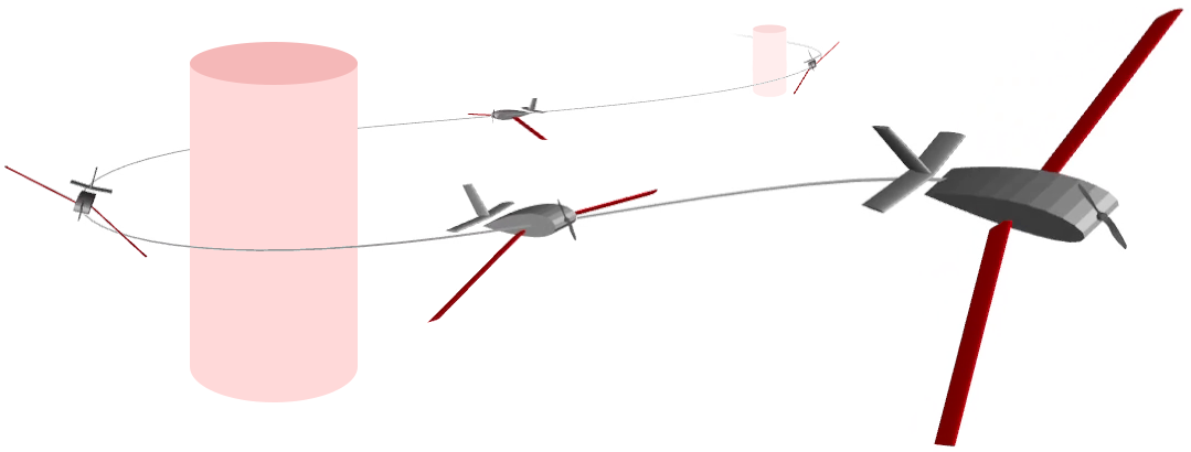
Figure 1: A co-designed morphing drone executing an agile manoeuvre.

The rest of this article is organised as follows. Section II introduces notation, presents the specificities of the morphing drone considered in this study, and recalls the basis of multibody modelling. Section III introduces the co-design method to evaluate the optimal drone. Section IV explains the morphing drone modelling. Section V presents the trajectory optimisation problem for solving desired scenarios. Section VI discusses the results obtained with the method and compares the performance of the morphing drone with a commercial fixed-wing drone. Finally, Section VII concludes this article.

II Background

II-A Notation

• ${I}_{n}{\in}\mathbb{R}^{n{\times}n}$ identity matrix, $\boldsymbol{0}_{n{\times}m}{\in}\mathbb{R}^{n{\times}m}$ zero matrix.

• $\text{SO}{\left(3\right)}:=\{R\in\mathbb{R}^{3{\times}3}\;|\;R^{\top}R{=}{I}_{3},\,\det{\left(R\right)}{=}1\}$

• $\mathcal{I}$ is the inertial frame; $\mathcal{C}$ is a generic body-fixed frame.

• $\boldsymbol{p}_{\mathcal{C}}\in\mathbb{R}^{3}$ denotes the origin of frame $\mathcal{C}$ expressed in $\mathcal{I}$.

• $R_{\mathcal{C}}\in\text{SO}{\left(3\right)}$ is the rotation matrix that transforms a $3$D vector expressed with the orientation of the frame $\mathcal{C}$ in a $3$D vector expressed in the frame $\mathcal{I}$. $R_{\mathcal{C}}{=}\begin{bmatrix}\boldsymbol{\hat{x}}_{\mathcal{C}}&\boldsymbol{\hat{y}}_{\mathcal{C}}&\boldsymbol{\hat{z}}_{\mathcal{C}}\end{bmatrix}$ with $\boldsymbol{\hat{x}}_{\mathcal{C}}$, $\boldsymbol{\hat{y}}_{\mathcal{C}}$, and $\boldsymbol{\hat{z}}_{\mathcal{C}}$ are the unit vectors of the frame axes.

• $\boldsymbol{\rho}_{\mathcal{C}}\in\mathbb{R}^{4}$ is the unit quaternion representation of $R_{\mathcal{C}}$.

• $\boldsymbol{\omega}_{\mathcal{C}}\in\mathbb{R}^{3}$ is the angular velocity of $\mathcal{C}$ relative to $\mathcal{I}$.

II-B Platform definition

The platform consists of a winged aircraft with left and right wings symmetrically connected to the fuselage by mechanical joints, which enable relative motion between the parts. The possible wing movements depend on the type of joint used to connect the wing and the fuselage (fig. 2). For instance, if we implement a joint with three actuated axis of rotation, we can obtain sweep, incidence, and dihedral variations. This solution provides a complete range of motion at the cost of higher weight and energy consumption. Alternatively, simpler and lighter joints with one or two servomotors can be used, but it becomes essential to determine the axis of rotation for achieving the desired behaviour. Although joints can be designed to produce translation motion, our study focuses on rotational movements only. Throughout the paper, we refer to this platform with the term morphing drone.

For sake of simplicity, we assume that the actuation of the morphing wing is sufficient to generate complex flight trajectories without the need of actuating wing ailerons and tail rudder and elevators. The propulsion unit consists of an electric propeller positioned at the front of the fuselage (frame $\mathcal{B}$ fig. 2).

Figure 2: Drone with morphing wings modelled as mechanical joints. The figure depicts the reference frames – coloured following the RGB convention – required for modelling.

II-C Floating Multibody System Modelling

The morphing drone can be modelled as a floating rigid multibody system with $n_{\text{j}}{+}1$ rigid bodies and $n_{\text{j}}$ one degrees-of-freedom (DoF) joints [25]. The configuration space $\mathbb{Q}$ of the system is the lie group $\mathbb{Q}{=}\mathbb{R}^{3}{\times}\text{SO}{\left(3\right)}{\times}\mathbb{R}^{n_{\text{j}}}$ represented by the pose (i.e. position and orientation) of the base frame $\mathcal{B}$, and the joint positions. The base frame is a frame rigidly connected to the fuselage, as depicted in fig. 2. The configuration $\boldsymbol{q}{=}\left(\boldsymbol{p}_{\mathcal{B}},R_{\mathcal{B}},\boldsymbol{s}\right)$ is a generic element of the configuration space. $\boldsymbol{p}_{\mathcal{B}}$ and $R_{\mathcal{B}}$ are the position and orientation of the base frame, and $\boldsymbol{s}$ are the joint positions. The tangent space of $\mathbb{Q}$ is the configuration space velocity $\mathbb{V}{=}\mathbb{R}^{3}{\times}\mathbb{R}^{3}{\times}\mathbb{R}^{n_{\text{j}}}$. The configuration velocity $\boldsymbol{\nu}{=}\left(\boldsymbol{\dot{p}}_{\mathcal{B}},\boldsymbol{\omega}_{\mathcal{B}},\boldsymbol{\dot{s}}\right)$ is a generic element of $\mathbb{V}$. $\boldsymbol{\dot{p}}_{\mathcal{B}}$ and $\boldsymbol{\omega}_{\mathcal{B}}$ are the linear and angular velocities of the base frame, and $\boldsymbol{\dot{s}}$ are the joint velocities. The position of a generic frame $\mathcal{C}$ attached to a link can be computed with the forward kinematic function $\text{FK}_{\boldsymbol{p}_{\mathcal{C}}}{\left(\cdot\right)}{:}\mathbb{Q}{\rightarrow}\mathbb{R}^{3}$. The linear and angular velocity of frame $\mathcal{C}$ can be computed via the Jacobian $J_{\mathcal{C}}\in\mathbb{R}^{6\times 6+n_{\text{j}}}$ which maps the configuration velocity to the Cartesian space, namely $\left(\boldsymbol{\dot{p}}_{\mathcal{C}};\boldsymbol{\omega}_{\mathcal{C}}\right)=J_{\mathcal{C}}\boldsymbol{\nu}$. The equation of motion, applying the Euler-Poincaré formalism  [26, Ch. 13.5], results in

$$M\left(\boldsymbol{q}\right)\boldsymbol{\dot{\nu}}+\boldsymbol{h}\left(\boldsymbol{q},\boldsymbol{\nu}\right)=\begin{bmatrix}\boldsymbol{0}_{1\times 6}&\boldsymbol{\tau}^{\top}\end{bmatrix}^{\top}+\boldsymbol{\mathrm{f}}^{\star}.$$ (1)

$M\left(\boldsymbol{q}\right)\in\mathbb{R}^{n_{\text{j}}{+}6{\times}n_{\text{j}}{+}6}$ is the mass matrix, $\boldsymbol{h}\left(\boldsymbol{q},\boldsymbol{\nu}\right)\in\mathbb{R}^{n_{\text{j}}+6}$ is the biased term which accounts for Coriolis, centrifugal effects, and gravity. $\boldsymbol{\tau}\in\mathbb{R}^{n_{\text{j}}}$ is the vector of joint torques, and $\boldsymbol{\mathrm{f}}^{\star}\in\mathbb{R}^{n_{\text{j}}+6}$ is the vector of generalised external wrenches.

II-D Wing Aerodynamic Modelling

A wing immersed in airflow causes deflections that generate stresses on the body. The net effect of the stresses integrated over the complete body surface results in aerodynamic forces and moments, which can be modelled as:

$$\boldsymbol{f}_{\boldsymbol{A}}=R_{\mathcal{W}}\frac{1}{2}\varrho_{\text{air}}\|\boldsymbol{v_{a}}\|^{2}S\begin{bmatrix}-C_{D}\left(\alpha,\beta,\mathit{Re},\mathit{Ma}\right)\\ C_{Y}\left(\alpha,\beta,\mathit{Re},\mathit{Ma}\right)\\ -C_{L}\left(\alpha,\beta,\mathit{Re},\mathit{Ma}\right)\end{bmatrix},$$ (2a)

$$\boldsymbol{\mu}_{\boldsymbol{A}}=R_{\mathcal{W}}\frac{1}{2}\varrho_{\text{air}}\|\boldsymbol{v_{a}}\|^{2}S\begin{bmatrix}b\,C_{l}\left(\alpha,\beta,\mathit{Re},\mathit{Ma}\right)\\ c\,C_{m}\left(\alpha,\beta,\mathit{Re},\mathit{Ma}\right)\\ b\,C_{n}\left(\alpha,\beta,\mathit{Re},\mathit{Ma}\right)\end{bmatrix}.$$ (2b)

$\mathcal{W}$ is the wind frame, $\varrho_{\text{air}}$ is the air density, $\boldsymbol{v_{a}}$ is the airspeed, $S$ is the planform area of the wing surface, and $c$ and $b$ are the mean aerodynamic chord and the wing span[27]. $C_{D}$, $C_{L}$, $C_{Y}$, $C_{l}$, $C_{m}$, and $C_{n}$ are the aerodynamic coefficients, $\alpha$ is the angle of attack, $\beta$ is the sideslip angle, $\mathit{Re}$ is the Reynolds number, and $\mathit{Ma}$ is the Mach number[28].

III Co-Design Methodology

The co-design method – illustrated in fig. 3 – identifies the conceptual design and control strategy of morphing drones considering energy consumption, agility, and hardware limitations. The design space is investigated with NSGA-II[29]. Each drone is evaluated with a fitness functions that measures the drone’s ability to succeed in a set of $n_{s}$ scenarios. We model the drone as a parametric multibody system subject to aerodynamics. A scenario is an environment with obstacles where the drone, given some initial condition, is asked to complete a series of checkpoints using trajectory optimisation.

Figure 3:  Multi-objective optimisation of drone morphology and control to reduce energy consumption and mission completion time in diverse flight environments. The multi-objective assessment (fitness) of each individual topology involves $n_{s}$ trajectory optimisations.

The parameters the method optimises are: $i)$ wing chord size and aspect ratio; $ii)$ wing static orientations; $iii)$ wing vertical and horizontal location; $iv)$ kinematic chain of the multibody system; $v)$ servomotor models; $vi)$ propulsion unit characteristics; and $vii)$ controller weight $\psi$ – discussed in section V-C. The wing static orientations are wing dihedral, incidence, and sweep angles when the joints are in the rest configuration, namely $\boldsymbol{s}=\boldsymbol{0}$. The wing’s vertical and horizontal location refers to the position of the frame $\mathcal{J}$ (depicted in fig. 2). The kinematic chain of the multibody system is the description of the mechanism with its links and joints. Specifically, the co-design method selects the number of joints interconnecting the fuselage and the wings, and it also identifies how these joints should be assembled, i.e., which axis of rotation must be actuated. The co-design method selects the servomotor models to actuate each joint and identifies the propulsion unit selecting the optimal motor-propeller combination. The design parameters are represented by an array of real values creating the chromosome. The fitness functions to be minimised are:

$$f_{1}=\sum_{i=1}^{n_{s}}\frac{\left(\text{energy}\right)_{i}}{n_{s}},\quad f_{2}=\sum_{i=1}^{n_{s}}\frac{\left(\text{time}\right)_{i}}{n_{s}}.$$

In case the scenario $i$ is unfeasible we assign $\left(\text{energy}\right)_{i}$ and $\left(\text{time}\right)_{i}$ a value of $10^{6}$.

IV Morphing Drone Modelling

The prediction of the drone behaviour relies on a mathematical model. In detail, the drones are modelled as floating multibody systems subject to significant aerodynamic forces that cannot be ignored. From the mechanical standpoint, the system comprises three primary links: the fuselage, the left-wing, and the right-wing, all assumed to be rigid. This section discusses joints, propulsion units, and aerodynamics modelling.

IV-A Mechanical Joints

The fuselage-wing connection consists of a mechanical $n$-DoFs joint created by combining $n$ one-DoF pin joints, each actuated with revolute DC servomotors with an integrated reduction system that enables a direct connection between the actuation and the links, eliminating the need for an additional reducer. We use the same joint configuration to connect both the left wing and right wing to the fuselage to have a symmetric design. The system comprises $2n$ pin joints and $2n$ servomotors. For simplicity, in the remainder of the paper, we use the word joints to refer to all $2n$ pin joints which are actuated with servomotors. If we consider a single revolute joint, the power consumption is estimated with a model:

$$W_{s}\left(\dot{s},\tau\right)=\dot{s}\tau+Rk_{v}^{2}\tau^{2},$$ (3)

$R$ is the electric servomotor resistance, $k_{v}$ is the motor constant velocity, $\dot{s}$ and $\tau$ are the joint velocity and torque.

IV-B Propulsion Unit

The propulsion unit is implemented with an electric propeller placed on the fuselage nose at frame $\mathcal{B}$, providing a positive force on $\boldsymbol{\hat{x}}_{\mathcal{B}}$ axis – see fig. 2. We neglect forces and moments in directions other than the $\boldsymbol{\hat{x}}_{\mathcal{B}}$ axis. The propeller power consumption is assumed to depend only on thrust $u$ as

$$W_{p}\left(u\right)=c_{0}+c_{1}u+c_{2}u^{2},$$ (4)

where $c_{0}$, $c_{1}$, $c_{2}$ are constants evaluated experimentally.

IV-C Aerodynamics Forces

The aerodynamic forces (and moments) acting on a multibody system are dependent on $\alpha$, $\beta$, $\mathit{Ma}$, $\mathit{Re}$, and $\boldsymbol{s}$. To simplify the aerodynamic analysis, we make these assumptions.

Assumption 1.

The effects of $\mathit{Ma}$ on the aerodynamic forces and moments are negligible in our flight regime $\left({\mathit{Ma}}{\ll}{1}\right)$, and the flow can be considered incompressible.

Assumption 2.

The aerodynamic forces and moments acting on the multibody system are approximated using the superposition principle, wherein interactions among bodies are neglected. The total forces and moments are calculated as the sum of forces and moments acting on each body.

Assumption 3.

The effects of rotational and unsteady motions of the platform on the surrounding airflow are negligible.

Assumption 1 removes the influence of $\mathit{Ma}$. Assumption 2 enables us to decompose the platform into three rigid bodies and evaluate the aerodynamic forces acting on each body independently of the joint configuration $\boldsymbol{s}$. For the generic body $i$, the forces and moments can be modelled with (2), and act on frame $\mathcal{A}_{i}$, depicted in fig. 2. Assumption 2 significantly decreases the number of required simulations or experiments. For instance, if our platform implements 3-DoF joints between fuselage and wings, without assumption 2 we would need to perform $10^{9}$ analysis. Thanks to assumption 2, the number of simulations drops to $2500$ for each body

IV-C1 Aerodynamic Coefficients Identification

we conducted aerodynamic simulations for all bodies using the $3$D uniform triangle panel Galerkin method with the software flow5[30]. The fuselage was represented with a naca0014 profile with a tail consisting of a horizontal and vertical stabiliser. The left and right wings were represented by a naca0009 profile with a constant chord. To capture the differences in the wing’s aspect ratio, we performed separate aerodynamic modelling for each possible aspect ratio. The aerodynamic simulations were performed in steady state configuration according to assumption 3, within the following parameter space: $i)$ $\alpha{=}\left[{-}10{:}2{:}10\right]\unit{}$, $\beta{=}\left[{-}30{:}2{:}30\right]\unit{}$, $\mathit{Re}{=}\left[2{:}1{:}15\right]{\times}10^{5}$ for the fuselage; and $ii)$ $\alpha{=}\left[{-}10{:}2{:}10\right]\unit{}$, $\beta{=}\left[{-}130{:}2{:}130\right]\unit{}$, $\mathit{Re}{=}\left[0.8{:}0.4{:}6.0\right]{\times}10^{5}$ for the wings. The ranges of the angle of attack $\alpha$, sideslip angle $\beta$, and Reynolds number $\mathit{Re}$ were selected based on the operating working conditions and the reliability range of the simulation software.

(a) $C_{D}$

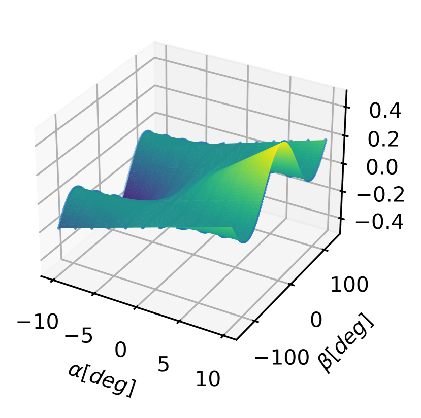
(b) $C_{L}$

Figure 4:  Aerodynamic coefficients naca0009 (taper ratio $1.0$, aspect ratio $2.0$, ${\mathit{Re}}{=}2{\times}10^{5}$). The blue dots are the flow5 data, while the surfaces represent the analytical functions that fit data.

After analysing the data, we used a linear regression approach to derive an analytical function that fits the data. We chose a candidate function consisting of the sum of sinusoidal terms and solved the regression problem using Lasso regularisation, which eliminates unnecessary terms [31]. The results for a wing are shown in fig. 4.

IV-D Equations of Motion

The dynamics of the studied morphing drone can be modelled with the equations presented in (1), where

$$\boldsymbol{\mathrm{f}}^{\star}=\sum_{i=1}^{3}J^{\top}_{\mathcal{A}_{i}}\left(\boldsymbol{q}\right)\begin{bmatrix}\boldsymbol{f}_{\boldsymbol{A}_{i}}\\ \boldsymbol{\mu}_{\boldsymbol{A}_{i}}\end{bmatrix}+J^{\top}_{\mathcal{B}}\left(\boldsymbol{q}\right)\begin{bmatrix}\boldsymbol{\hat{x}}_{\mathcal{B}}\left(\boldsymbol{q}\right)\\ \boldsymbol{0}_{3\times 1}\end{bmatrix}u.$$ (5)

The aerodynamic forces and moments are evaluated with (2) employing the aerodynamic coefficients identified with procedure discussed in section IV-C1.

V Trajectory Optimisation

The co-design method assesses drones’ ability in complete scenarios. The trajectory optimisation evaluates the desired actuation inputs $\left(\boldsymbol{\tau},u\right)$ to navigate the drone in a given scenario being optimal according to a user metric. The scenarios we consider involve reaching target locations with a desired attitude while avoiding obstacles. The possible metrics that can be minimised include energy consumption and the time to complete the scenario. The trajectory optimisation is transcribed using a direct multiple-shooting method, discretised in $N$ knots, and formulated as an optimisation problem with cost function and constraints.

V-A Decision Variables

The decision variables of the optimisation problem are:

• joint configurations and torques $\boldsymbol{s}$, $\boldsymbol{\dot{s}}$, $\boldsymbol{\ddot{s}}$, $\boldsymbol{\tau}$, $\boldsymbol{\dot{\tau}}$;

• base position and attitude $\boldsymbol{p}_{\mathcal{B}}$, $\boldsymbol{\rho}_{\mathcal{B}}$, $\boldsymbol{\dot{p}}_{\mathcal{B}}$, $\boldsymbol{\omega}_{\mathcal{B}}$, $\boldsymbol{\ddot{p}}_{\mathcal{B}}$, $\boldsymbol{\dot{\omega}}_{\mathcal{B}}$;

• propeller thrust $u$, $\dot{u}$; and

• time interval between knots $\Delta t$.

V-B Constraints

V-B1 Initial Conditions

we specify in the initial knot

$$\boldsymbol{p}_{\mathcal{B}}{\left[0\right]}{=}\boldsymbol{p}_{\mathcal{B}0},\hskip 2.9pt\boldsymbol{\rho}_{\mathcal{B}}{\left[0\right]}{=}\boldsymbol{\rho}_{\mathcal{B}0},\hskip 2.9pt\boldsymbol{\dot{p}}_{\mathcal{B}}{\left[0\right]}{=}\boldsymbol{\dot{p}}_{\mathcal{B}0},\hskip 2.9pt\boldsymbol{\omega}_{\mathcal{B}}{\left[0\right]}{=}\boldsymbol{\omega}_{\mathcal{B}0},$$ (6a)

$$\boldsymbol{s}{\left[0\right]}{=}\boldsymbol{s}_{0},\hskip 4.0pt,\boldsymbol{\dot{s}}{\left[0\right]}{=}\boldsymbol{\dot{s}}_{0},\hskip 4.0pt,\boldsymbol{\ddot{s}}{\left[0\right]}{=}\boldsymbol{\ddot{s}}_{0}.$$ (6b)

V-B2 Hardware and Physical Limits

we bound the decision variable for all the $N$ knots. For simplicity, the next constraints are expressed w.r.t. the generic knot $k$. For the joints and the propeller, we require:

$$\boldsymbol{s}_{\text{min}}{\leq}\boldsymbol{s}{\left[k\right]}{\leq}\boldsymbol{s}_{\text{max}},\hskip 4.0pt\boldsymbol{\dot{s}}_{\text{min}}{\leq}\boldsymbol{\dot{s}}{\left[k\right]}{\leq}\boldsymbol{\dot{s}}_{\text{max}},\hskip 4.0pt\boldsymbol{\ddot{s}}_{\text{min}}{\leq}\boldsymbol{\ddot{s}}{\left[k\right]}{\leq}\boldsymbol{\ddot{s}}_{\text{max}},$$ (7a)

$$\boldsymbol{\tau}_{\text{min}}{\leq}\boldsymbol{\tau}{\left[k\right]}{\leq}\boldsymbol{\tau}_{\text{max}},\hskip 4.0ptu_{\text{min}}{\leq}u{\left[k\right]}{\leq}u_{\text{max}}.$$ (7b)

To ensure the continuity of the control inputs, we bound:

$$\boldsymbol{\dot{\tau}}_{\text{min}}\leq\boldsymbol{\dot{\tau}}{\left[k\right]}\leq\boldsymbol{\dot{\tau}}_{\text{max}},\hskip 4.0pt\dot{u}_{\text{min}}\leq\dot{u}{\left[k\right]}\leq\dot{u}_{\text{max}}.$$ (8)

The aerodynamic angles are constrained to remain within the reliable range of the model discussed in section IV-C:

$$\alpha_{\text{min}}\leq\alpha{\left[k\right]}\leq\alpha_{\text{max}},\hskip 4.0pt\beta_{\text{min}}\leq\beta{\left[k\right]}\leq\beta_{\text{max}}.$$ (9)

Lastly, we constrain the time increment to be positive and lower than a threshold to prevent integration error, as:

$$0\leq\Delta t{\left[k\right]}\leq\Delta t_{\text{max}}.$$ (10)

V-B3 Obstacles Avoidance

we require a positive distance between the drone and any obstacle. We model the obstacles with $n_{\text{obs}}$ primitive shapes describable by a set $\mathcal{S}_{\mathcal{O}}$. We identify $n_{\text{f}}$ significant points on the drone. For the generic point f we must ensure

$$\boldsymbol{p}_{\text{f}}{\left[k\right]}{=}\text{FK}_{\boldsymbol{p}_{\text{f}}}{\left(\boldsymbol{q}\right)}{\left[k\right]}\notin\mathcal{S}_{\mathcal{O}}\quad{\forall}k{\in}\left[0{,}{...}{N}\right].$$ (11)

V-B4 Checkpoints

we ask the drone to complete $n_{\text{cp}}$ checkpoints. A generic checkpoint $P$ is defined as a set $\mathcal{S}_{P}{=}\left(\boldsymbol{p}_{P}{,}\boldsymbol{\rho}_{P}{,}\boldsymbol{\dot{p}}_{P}{,}\boldsymbol{\omega}_{P}\right)$ in which the drone configuration should lie at the knot $k_{P}$, i.e.,

$$\left(\boldsymbol{p}_{\mathcal{B}}{\left[k_{P}\right]},\boldsymbol{\rho}_{\mathcal{B}}{\left[k_{P}\right]},\boldsymbol{\dot{p}}_{\mathcal{B}}{\left[k_{P}\right]},\boldsymbol{\omega}_{\mathcal{B}}{\left[k_{P}\right]}\right)\in\mathcal{S}_{P}.$$ (12)

The timing of each checkpoint is not defined by selecting the knot because $\Delta t$ is a decision variable.

V-B5 Decision Variables Integration

we integrate the time-varying optimisation variables $\boldsymbol{s}$, $\boldsymbol{\dot{s}}$, $\boldsymbol{\tau}$, $u$, $\boldsymbol{p}_{\mathcal{B}}$, $\boldsymbol{\dot{p}}_{\mathcal{B}}$, and $\boldsymbol{\omega}_{\mathcal{B}}$ using the backward Euler method.

For $\boldsymbol{\rho}_{\mathcal{B}}$, we require

$$\boldsymbol{\rho}_{\mathcal{B}}{\left[k{+}1\right]}{=}\text{Exp}\left(\boldsymbol{\omega}{\left[k{+}1\right]}\Delta t{\left[k\right]}\right)\boldsymbol{\rho}_{\mathcal{B}}{\left[k\right]}.\\$$ (13)

$\text{Exp}\left(\cdot\right)$ implements the exponential operator which maps a $3$D angular velocity vector to a unit quaternion [32].

V-B6 Multibody Dynamics

we impose the dynamics that follow the modelling discussed in section IV, i.e.

$$M\left(\boldsymbol{q}{\left[k\right]}\right)\boldsymbol{\dot{\nu}}{\left[k\right]}+\boldsymbol{h}\left(\boldsymbol{q}{\left[k\right]},\boldsymbol{\nu}{\left[k\right]}\right)=\begin{bmatrix}\boldsymbol{0}_{6\times 1}\\ \boldsymbol{\tau}{\left[k\right]}\end{bmatrix}+\boldsymbol{\mathrm{f}}^{\star}$$ (14)

for $k\in\left[0,...N\right]$. $\boldsymbol{\mathrm{f}}^{\star}$ is computed with (5). $\alpha$, $\beta$, $\mathit{Re}$, and $\boldsymbol{v_{a}}$ are computed for each body exploiting the kinematic chain.

V-C Cost Function

The cost function minimises a combination of time and energy consumption regulated by the weight $\psi$, namely:

$$f_{c}=\psi\sum_{k}^{N}\Delta t+\sum_{k}^{N}\left[W_{p}\left(u\right)+\sum_{j}^{n_{\text{j}}}W_{s_{j}}\left(\boldsymbol{\dot{s}},\boldsymbol{\tau}\right)\right]\Delta t.$$ (15)

V-D Optimisation Problem

The complete optimisation problem is formulated as

$$\text{min}_{\boldsymbol{\chi}} \psi\cdot\text{time}+\text{energy}\quad$$ eq. (15) (16)

s.t. initial conditions eq. (6)

hardware & physical limits eqs. (7) to (10)

obstacles avoidance eq. (11)

checkpoints eq. (12)

integration eq. (13)

system dynamics eq. (14)

where $\boldsymbol{\chi}$ collects all the decision variables for all knots.

VI Results

Here, we test the method by exploring the co-design of an agile drone capable of performing complex manoeuvres. Then, we validate the method by comparing the performance of the co-designed morphing drones with that of a commercial fixed-wing drone.

VI-A Co-Design Method

The assessment of the co-design method requires the development of a co-design framework. Our frameworkis designed to enable users to: $i)$ define scenarios; $ii)$ modify trajectory optimisation formulation; and $iii)$ provide preferred aerodynamic models. The trajectory optimisation is implemented using CasADi and solved using Ipopt [33], with the ma27 linear solver [34]. The multibody system modelling is implemented using the ADAM library [35]. NSGA-II is implemented using DEAP library [36] with an evolutionary process characterised by a population of $100$ individuals, single-point crossover ($p{=}90{\%}$), random mutation ($p{=}6{\%}$), and a stop criteria after $100$ generations.

We investigated the co-design of an agile drone capable of flying in airspace with obstacles that require complex manoeuvres, selecting five scenarios ($n_{s}{=}5$) for fitness evaluation. Each scenario involves a slalom manoeuvre between two obstacles to evaluate the capability of changing directions. The five scenarios share the same checkpoints and obstacles but vary in the drone’s initial conditions, i.e., forward velocity ($8{\text{-}}12\unit{{}{/}{}}$) and pitch orientation (${-}5{\text{-}}5\unit{}$). The obstacles are cylinders with infinite lengths and a ground plane. The final target is $\boldsymbol{p}_{\mathcal{B}}{=}\left(60,0,0\right)\unit{{}}$ with $\boldsymbol{\dot{p}}_{\mathcal{B}}{=}\left(10,0,0\right)\unit{{}{/}{}}$. Two intermediate checkpoints are located near the obstacles. The wind speed is $\left(-1,0,0\right)\unit{{}{/}{}}$. A scenario is depicted in fig. 6.

The co-design method was run eight times on a machine with an Intel Xeon Silver 4214 CPU ($48$ cores). The average runtime for each execution was approximately $\qty{31.9}{}$. $6400$ different individuals were analysed for each run, and $32000$ trajectory optimisation problems were solved. In all tests, the fuselage and wings are assumed to be made of Expanded Polystyrene. The fuselage has a length of $\qty{0.75}{}$, a width of $\qty{0.1}{}$, and it holds a payload of $\qty{0.35}{{\kilo}}$ to account for the battery and the electronics. The wing design parameters, identified by the co-design method, are listed in table I. The method selects the propulsion unit from an online database[37] and similarly chooses the servomotors to actuate the wings from a database of off-the-shelf Dynamixel servomotors.

TABLE I:  Wing design space of the co-design method.

Wing Design Parameter		min	max	step
gray!15 chord size	${\unit{}}$	$0.1$	$0.4$	$0.05$
aspect ratio	$\cdot$	$2$	$5$	$0.5$
gray!15 wing static orientations	${\unit{}}$	$-10$	$10$	$2$
vertical location	${\unit{}}$	$-0.03$	$0.03$	$0.01$
gray!15 horizontal location	${\unit{}}$	$-0.4$	$-0.1$	$0.05$

Figure 5:  Optimal Pareto front evaluated by the co-design optimisation method. Each line represents the output of a single run. The markers identify the individuals analysed in fig. 6, fig. 7, and section VI-B. bix3 is a commercial fixed-wing drone later used for validation.

The Pareto fronts, evaluated by the co-design method in the eight runs, are shown in fig. 5. The resulting drones share common characteristics: a negative static dihedral, positive wing static angle of attack, wings mounted in the upper part of the fuselage, and a chord length of $\qty{0.2}{{}}$. Agile drones tend to have a lower aspect ratio, a powerful propulsion unit, higher gain $\psi$, and are often equipped with three servomotors per wing. Differently, energy-efficiency drones present opposite characteristics and are usually designed with two servomotors per wing (sweep & incidence) or, in some cases, only one (incidence). In terms of servomotor models, the dihedral motors are usually more powerful ($\tau_{\text{max}}{=}\qty{2.7}{{{}}{{}}}$) than sweep and incidence servomotors ($\tau_{\text{max}}{=}\qty{0.4}{{}{}}$). The drone’s weight is influenced by wing size, number of joints, and servomotor models. As a result, energy-efficient drones tend to have lower mass ($\qty{0.8}{{\kilo}}$) than their agile counterparts ($\qty{1}{{\kilo}}$).

Figure 5 shows four co-designed drones labelled as opt1, opt2, opt3, and opt4. opt1 is equipped with a single joint per wing for actuating the incidence angle, wing aspect ratio $3.5$, and has a propeller with $u_{\text{max}}{=}\qty{4}{{}}$. opt2 has two revolute joints to actuate sweep and incidence, wing aspect ratio $3.5$, and $u_{\text{max}}{=}\qty{4}{{}}$. opt3 incorporates three revolute joints to actuate dihedral, sweep, and incidence, wing aspect ratio $4.5$, and $u_{\text{max}}{=}\qty{10}{{}}$. opt4 has two revolute joints to actuate incidence and dihedral, wing aspect ratio $3.5$, and $u_{\text{max}}{=}\qty{10}{{}}$. Figures 6 and 7 report the trajectories of the opt drones during a scenario with an initial forward velocity of $10\unit{{}{/}{}}$ and zero initial pitch orientation.

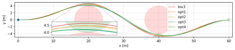
Figure 6:  Optimal trajectories of the opt drones. The green and red areas represent checkpoints and obstacles, respectively. The drones follow similar paths except near obstacles, where the more agile solutions approach with lower clearance and higher speed (see fig. 7).

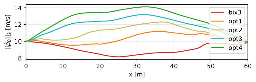
Figure 7:  Velocity profiles of co-designed drones during slalom trajectory. opt3 and opt4 achieve higher speeds and complete the scenario more quickly.

VI-B Co-Design Validation

In section VI-A, we tested the co-design method designing an agile drone capable of avoiding obstacles by studying $n_{s}{=}5$ scenarios; however, drones may operate in different conditions. We now assess the capabilities of the optimal drones in environments different from the optimised ones. In our analysis, we include the four opt drones represented in fig. 5; and a commercial drone with fixed-wing and control surfaces called H-King Bixler3 which serves as a baseline as it is of similar weight and size as the opt drones. We refer to this drone as bix3. The aerodynamic model of bix3 was obtained by combining the wind tunnel results with the data presented in [5]. bix3 has a propeller which can provide $u_{\text{max}}{=}\qty{7}{{}}$, a total wingspan of $\qty{1.55}{}$, and weights $\qty{1012}{}$ when equipped with sensors for autonomous flight[38].

Figure 8:  Parametric scenario to validate the co-design method. The drone starts at the blue sphere and must reach two (green) checkpoints while avoiding obstacles (red spheres).

bix3 and opt drones are evaluated in a common parametric scenario depicted in fig. 8. For each drone, we performed $810$ simulations by varying the parameters $d$, $\gamma$, $r$, $v_{x}$, and $\theta_{\text{p}}$ in all possible configurations. $v_{x}$ is the forward velocity, and $\theta_{\text{p}}$ is the pitch orientation. The results of the $810{\times}5$ simulations are shown in fig. 9. Co-designed drones exhibit a decrease in average energy consumption by $40{\text{-}}73{\%}$ and a decrease in time to complete the scenario by $21{\text{-}}34{\%}$ compared to bix3. Therefore, the resulting opt drones outperform the commonly used commercial platform in agility and energy efficiency in our tested scenarios.

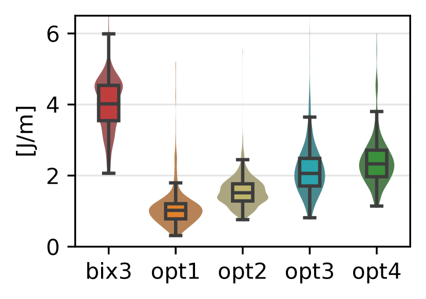
(a) energy normalised

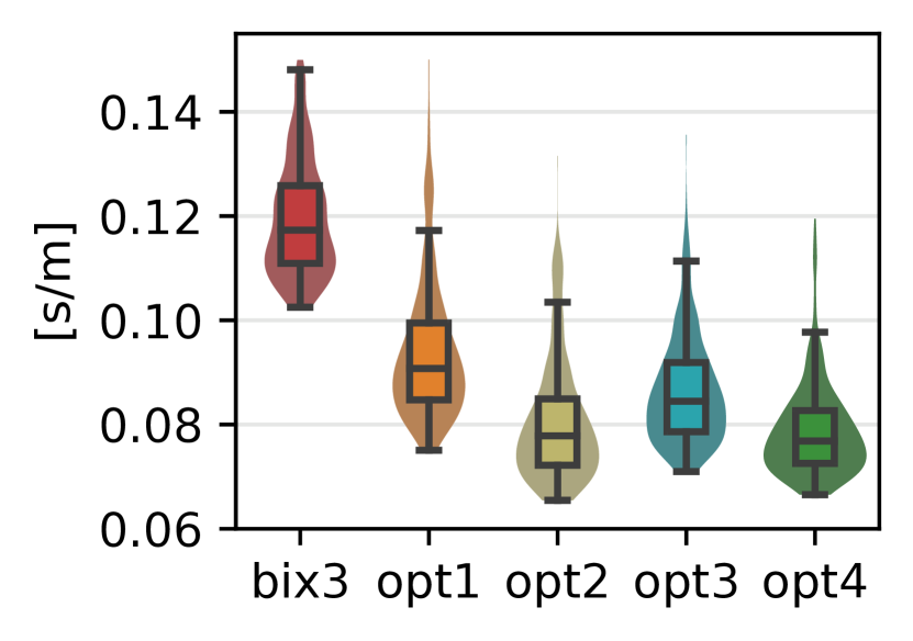
(b) time normalised

Figure 9:  Results of the validation of co-design methodology. Energy consumption and time are divided by distance $d$ for comparing scenarios with different characteristics.

VII Conclusions

Co-design methods can assist engineers in developing more efficient drones, but existing methods are inadequate for drones with morphing wings. This paper addresses this gap by proposing a co-design methodology that identifies drone topology, actuation, morphing wing strategy, and controller parameters. Our method relies on a parametric modelling approach, trajectory optimisation, and a multi-objective optimisation algorithm.

The method was tested for the co-design of morphing topology and control in five airspace scenarios that systematically vary in the position of intervening obstacles to maximise agility and minimise energy consumption. However, the method could be used also with other objectives and different scenarios.

Morphing drones’ aerodynamics were modelled with an approach valid at low angles of attack – forcing us to limit the wing range of movements – and we neglected the interactions between wings and fuselage to reduce computational complexities. Relaxing these assumptions would lead to a more realistic model that can unlock aggressive manoeuvres.

Future work could include the integration of a dynamic simulator to study wind disturbance rejection and the enlargement of the design space to include propeller positioning, battery selection, and other fuselage and tail configurations.

The topology and control co-design method described here could be used to assist aircraft engineers in the initial design phase of agile and energy-efficient morphing drones that mission-specific costs and constraints.

References

- [1] D. Floreano and R. J. Wood, “Science, technology and the future of small autonomous drones,” nature, vol. 521, no. 7553, pp. 460–466, 2015.
- [2] V. Kumar and N. Michael, “Opportunities and challenges with autonomous micro aerial vehicles,” The International Journal of Robotics Research, vol. 31, no. 11, pp. 1279–1291, 2012.
- [3] A. Sofla, S. Meguid, K. Tan, and W. Yeo, “Shape morphing of aircraft wing: Status and challenges,” Materials & Design, vol. 31, no. 3, pp. 1284–1292, 2010. [Online]. Available: https://www.sciencedirect.com/science/article/pii/S0261306909004968
- [4] A. A. Paranjape, S.-J. Chung, and J. Kim, “Novel dihedral-based control of flapping-wing aircraft with application to perching,” IEEE Transactions on Robotics, vol. 29, no. 5, pp. 1071–1084, 2013.
- [5] A. Waldock, C. Greatwood, F. Salama, and T. Richardson, “Learning to perform a perched landing on the ground using deep reinforcement learning,” Journal of intelligent & robotic systems, vol. 92, pp. 685–704, 2018.
- [6] E. Ajanic, M. Feroskhan, V. Wüest, and D. Floreano, “Sharp turning maneuvers with avian-inspired wing and tail morphing,” Communications Engineering, vol. 1, no. 1, p. 34, 2022.
- [7] R. Vos, R. Barrett, R. de Breuker, and P. Tiso, “Post-buckled precompressed elements: a new class of control actuators for morphing wing uavs,” Smart materials and structures, vol. 16, no. 3, p. 919, 2007.
- [8] Y. Ke, H. Yu, C. Chi, M. Yue, and B. M. Chen, “A systematic design approach for an unconventional uav j-lion with extensible morphing wings,” in 2016 12th IEEE International Conference on Control and Automation (ICCA). IEEE, 2016, pp. 44–49.
- [9] B. Jenett, S. Calisch, D. Cellucci, N. Cramer, N. Gershenfeld, S. Swei, and K. C. Cheung, “Digital morphing wing: active wing shaping concept using composite lattice-based cellular structures,” Soft robotics, vol. 4, no. 1, pp. 33–48, 2017.
- [10] D. Raymer, Aircraft design: a conceptual approach. American Institute of Aeronautics and Astronautics, Inc., 2012.
- [11] M. H. Sadraey, Aircraft design: A systems engineering approach. John Wiley & Sons, 2012.
- [12] A. J. Keane, A. Sóbester, and J. P. Scanlan, Small unmanned fixed-wing aircraft design: a practical approach. John Wiley & Sons, 2017.
- [13] T. Chen, Z. He, and M. Ciocarlie, “Co-designing hardware and control for robot hands,” Science Robotics, vol. 6, no. 54, p. eabg2133, 2021.
- [14] M. Garcia-Sanz, “Control co-design: an engineering game changer,” Advanced Control for Applications: Engineering and Industrial Systems, vol. 1, no. 1, p. e18, 2019.
- [15] C. Sartore, L. Rapetti, and D. Pucci, “Optimization of humanoid robot designs for human-robot ergonomic payload lifting,” in 2022 IEEE-RAS 21st International Conference on Humanoid Robots (Humanoids). IEEE, 2022, pp. 722–729.
- [16] G. Fadini, T. Flayols, A. Del Prete, and P. Souères, “Simulation aided co-design for robust robot optimization,” IEEE Robotics and Automation Letters, vol. 7, no. 4, pp. 11 306–11 313, 2022.
- [17] G. Bravo-Palacios and P. M. Wensing, “Large-scale admm-based co-design of legged robots,” in 2022 IEEE/RSJ International Conference on Intelligent Robots and Systems (IROS). IEEE, 2022, pp. 8842–8849.
- [18] T. Chen, Z. He, and M. Ciocarlie, “Hardware as policy: Mechanical and computational co-optimization using deep reinforcement learning,” arXiv preprint arXiv:2008.04460, 2020.
- [19] A. Sathuluri, A. V. Sureshbabu, and M. Zimmermann, “Robust co-design of robots via cascaded optimisation,” in 2023 IEEE International Conference on Robotics and Automation (ICRA). IEEE, 2023, pp. 11 280–11 286.
- [20] T. Du, A. Schulz, B. Zhu, B. Bickel, and W. Matusik, “Computational multicopter design,” ACM Transactions on Graphics, 2016.
- [21] F. Schiano, P. M. Kornatowski, L. Cencetti, and D. Floreano, “Reconfigurable drone system for transportation of parcels with variable mass and size,” IEEE Robotics and Automation Letters, vol. 7, no. 4, pp. 12 150–12 157, 2022.
- [22] L. Carlone and C. Pinciroli, “Robot co-design: beyond the monotone case,” in 2019 International Conference on Robotics and Automation (ICRA). IEEE, 2019, pp. 3024–3030.
- [23] A. Zhao, T. Du, J. Xu, J. Hughes, J. Salazar, P. Ma, W. Wang, D. Rus, and W. Matusik, “Automatic co-design of aerial robots using a graph grammar,” in 2022 IEEE/RSJ International Conference on Intelligent Robots and Systems (IROS). IEEE, 2022, pp. 11 260–11 267.
- [24] E. De Margerie, J.-B. Mouret, S. Doncieux, and J.-A. Meyer, “Artificial evolution of the morphology and kinematics in a flapping-wing mini-uav,” Bioinspiration & biomimetics, vol. 2, no. 4, p. 65, 2007.
- [25] R. Featherstone, Rigid body dynamics algorithms. Springer, 2014.
- [26] J. E. Marsden and T. S. Ratiu, Introduction to mechanics and symmetry: a basic exposition of classical mechanical systems. Springer Science & Business Media, 2013, vol. 17.
- [27] R. W. Beard and T. W. McLain, Small unmanned aircraft: Theory and practice. Princeton university press, 2012.
- [28] K. P. Valavanis and G. J. Vachtsevanos, Handbook of unmanned aerial vehicles. Springer, 2015, vol. 1.
- [29] K. Deb, A. Pratap, S. Agarwal, and T. Meyarivan, “A fast and elitist multiobjective genetic algorithm: Nsga-ii,” IEEE transactions on evolutionary computation, vol. 6, no. 2, pp. 182–197, 2002.
- [30] Andre Deperrois. (2022) flow5. [Online]. Available: https://flow5.tech/
- [31] R. Tibshirani, “Regression shrinkage and selection via the lasso,” Journal of the Royal Statistical Society: Series B (Methodological), vol. 58, no. 1, pp. 267–288, 1996.
- [32] J. Sola, J. Deray, and D. Atchuthan, “A micro lie theory for state estimation in robotics,” arXiv preprint arXiv:1812.01537, 2018.
- [33] A. Wächter and L. T. Biegler, “On the implementation of an interior-point filter line-search algorithm for large-scale nonlinear programming,” Mathematical programming, vol. 106, pp. 25–57, 2006.
- [34] STFC Rutherford Appleton Laboratory. (2002) Hsl. a collection of fortran codes for large scale scientific computation. [Online]. Available: http://www.hsl.rl.ac.uk/
- [35] G. L’Erario, G. Nava, G. Romualdi, F. Bergonti, V. Razza, S. Dafarra, and D. Pucci, “Whole-body trajectory optimization for robot multimodal locomotion,” in 2022 IEEE-RAS 21st International Conference on Humanoid Robots (Humanoids), 2022, pp. 651–658.
- [36] F.-A. Fortin, F.-M. De Rainville, M.-A. G. Gardner, M. Parizeau, and C. Gagné, “Deap: Evolutionary algorithms made easy,” The Journal of Machine Learning Research, vol. 13, no. 1, pp. 2171–2175, 2012.
- [37] Tyto Robotics. (2023) Motor and propeller database. [Online]. Available: https://database.rcbenchmark.com/
- [38] V. Wüest, E. Ajanic, M. Müller, and D. Floreano, “Accurate vision-based flight with fixed-wing drones,” in 2022 IEEE/RSJ International Conference on Intelligent Robots and Systems (IROS). IEEE, 2022, pp. 12 344–12 351.