Observational constraints on interactions between dark energy and dark matter
with momentum and energy transfers

Abstract

We place observational constraints on a dark energy (DE) model in which a quintessence scalar field $\phi$ is coupled to dark matter (DM) through momentum and energy exchanges. The momentum transfer is weighed by an interaction between the field derivative and DM four velocity with a coupling constant $\beta$, whereas the energy exchange is characterized by an exponential scalar-field coupling to the DM density with a coupling constant $Q$. A positive coupling $\beta$ leads to the suppression for the growth of DM density perturbations at low redshifts, whose property offers a possibility for resolving the $\sigma_{8}$ tension problem. A negative coupling $Q$ gives rise to a $\phi$-matter-dominated epoch, whose presence can reduce the sound horizon around the Cosmic Microwave Background (CMB) decoupling epoch. Using the data of Planck 2018, 12-th Sloan Digital Sky Survey, Phantheon supernovae samples, and 1-year dark energy survey, we find that the two couplings are constrained to be $\beta=0.417^{+1.592}_{-0.307}$ and $Q=-0.036^{+0.036}_{-0.010}$ at 68 % confidence level (CL). Thus, there is an interesting observational signature of the momentum exchange ($\beta\neq 0$) between DE and DM, with a peak of the probability distribution of the energy transfer coupling at $Q<0$.

I Introduction

Revealing the origin of the dark sector in our Universe is an important challenge for the modern cosmology Jungman et al. (1996); Bertone et al. (2005); Peebles and Ratra (2003); Copeland et al. (2006); Silvestri and Trodden (2009); Kase and Tsujikawa (2019); Ezquiaga and Zumalacárregui (2018). Dark energy (DE) accelerates the current Universe, while cold dark matter (CDM) is the main source for the formation of large-scale structures. The origin of DE can be a cosmological constant $\Lambda$ Weinberg (1989); Sahni and Starobinsky (2000); Padmanabhan (2003); Carroll (2001), but it is theoretically challenging to naturally explain its small value from the vacuum energy arising from particle physics Martin (2012); Padilla (2015). Instead, there have been many attempts for constructing DE models with dynamical propagating degrees of freedom such as scalar fields, vector fields, and massive gravitons (see Refs. De Felice and Tsujikawa (2010); Clifton et al. (2012); Joyce et al. (2015); Koyama (2016); Ishak (2019); Heisenberg (2019) for reviews). Among them, the scalar-field DE, which is dubbed quintessence Fujii (1982); Ford (1987); Ratra and Peebles (1988); Wetterich (1988); Chiba et al. (1997); Ferreira and Joyce (1997); Caldwell et al. (1998); Zlatev et al. (1999), is one of the simplest models which can be distinguished from the cosmological constant through its time-varying equation of state (EOS) $w_{\rm DE}$.

From the observational side, we have not yet found compelling evidence that quintessence is favored over the cosmological constant. In particular, the joint analysis based on the data of supernovae Ia (SN Ia), baryon acoustic oscillations (BAO), and the cosmic microwave background (CMB) showed that the quintessence EOS needs to be close to $-1$ at low redshifts Chiba et al. (2013); Tsujikawa (2013); Durrive et al. (2018); Aghanim et al. (2020a); Akrami et al. (2019). Hence it is difficult to distinguish between quintessence and $\Lambda$ from the information of $w_{\rm DE}$ alone. At the level of perturbations, the $\Lambda$CDM model has a so-called $\sigma_{8}$ tension for the amplitude of matter density contrast between the Planck CMB data Aghanim et al. (2020a) and low-redshift probes like shear-lensing Heymans et al. (2012); Hildebrandt et al. (2017); Abbott et al. (2018a) and redshift-space distortions Samushia et al. (2014); Macaulay et al. (2013). For both $\Lambda$ and quintessence, the effective gravitational coupling $G_{\rm eff}$ on scales relevant to the growth of large-scale structures is equivalent to the Newton constant $G$. Then, the problem of the $\sigma_{8}$ tension cannot be addressed by quintessence either. Moreover, for both $\Lambda$ and quintessence, there is the tension of today’s Hubble expansion rate $H_{0}$ between the CMB data and low-redshift measurements Aghanim et al. (2020b); Riess et al. (2018); Wong et al. (2020); Riess et al. (2021); Verde et al. (2019); Di Valentino et al. (2021); Perivolaropoulos and Skara (2021); Freedman (2021).

If we allow for a possibility of interactions between DE and DM, the cosmic expansion and growth histories can be modified in comparison to the $\Lambda$CDM model. One example of such couplings corresponds to an energy exchange between DE and DM through an interacting Lagrangian $L_{\rm E}=-(e^{Q\phi/M_{\rm Pl}}-1)\rho_{c}$ Wetterich (1995); Amendola (2000); Frusciante et al. (2019); Kase and Tsujikawa (2020a), where $Q$ is a coupling constant, $M_{\rm Pl}$ is the reduced Planck mass, and $\rho_{c}$ is the CDM density. The similar type of couplings arises from Brans-Dicke theories Brans and Dicke (1961) after transforming the Jordan-frame action to that in the Einstein frame Amendola (1999); Khoury and Weltman (2004); Tsujikawa et al. (2008). In the presence of such an energy transfer, it is possible to realize a so-called $\phi$-matter-dominated epoch ($\phi$MDE) Amendola (2000) in which the DE (scalar field) density parameter takes a nonvanishing constant value $\Omega_{\rm DE}=2Q^{2}/3$. The presence of the $\phi$MDE can reduce the sound horizon at CMB decoupling Pettorino (2013); Ade et al. (2016); Gómez-Valent et al. (2020), which may offer a possibility for alleviating the $H_{0}$ tension. On the other hand, the effective gravitational coupling of CDM is given by $G_{\rm eff}=G(1+2Q^{2})$ Amendola (2004); Tsujikawa (2007), which is larger than $G$. This property is not welcome for reducing the $\sigma_{8}$ tension, as we require that $G_{\rm eff}<G$ to address this problem.

The scalar field can also mediate the momentum exchange with CDM through a scalar product $Z=u_{c}^{\mu}\nabla_{\mu}\phi$ Pourtsidou et al. (2013); Boehmer et al. (2015); Skordis et al. (2015); Koivisto et al. (2015); Pourtsidou and Tram (2016); Dutta et al. (2017); Linton et al. (2018); Kase and Tsujikawa (2020a, b); Chamings et al. (2020); Amendola and Tsujikawa (2020); Kase and Tsujikawa (2020c); Linton et al. (2022), where $u_{c}^{\mu}$ is a CDM four velocity and $\nabla_{\mu}\phi$ is a covariant derivative of $\phi$. If we consider an interacting Lagrangian of the form $L_{\rm M}=\beta Z^{2}$, where $\beta$ is a coupling constant, the modification to the background equations arises only through a change of the kinetic term $\dot{\phi}^{2}/2\to(1+2\beta)\dot{\phi}^{2}/2$ in the density and pressure of $\phi$ Pourtsidou et al. (2013); Pourtsidou and Tram (2016). At the level of perturbations, the Euler equation is modified by the momentum transfer, while the continuity equation is not affected. For $\beta>0$, the conditions for the absence of ghosts and Laplacian instabilities of scalar and tensor perturbations are consistently satisfied Kase and Tsujikawa (2020b). In this case, the effective gravitational coupling of CDM is smaller than $G$ at low redshifts Pourtsidou et al. (2013); Pourtsidou and Tram (2016); Kase and Tsujikawa (2020a, b). Then, there is an intriguing possibility for reducing the $\sigma_{8}$ tension by the momentum transfer Pourtsidou and Tram (2016); Linton et al. (2018); Chamings et al. (2020); Linton et al. (2022).

An interacting model of DE and DM with both momentum and energy transfers was proposed in Ref. Amendola and Tsujikawa (2020) as a possible solution to the problems of $\sigma_{8}$ and $H_{0}$ tensions. This is described by the interacting Lagrangian $L_{\rm int}=\beta Z^{2}-(e^{Q\phi/M_{\rm Pl}}-1)\rho_{c}$ with a canonical scalar field $\phi$ having a potential $V(\phi)$. Since the model has an explicit Lagrangian, the perturbation equations of motion are unambiguously fixed by varying the corresponding action with respect to the perturbed variables. We would like to stress that this is not the case for many interacting DE and DM models in which the background equations alone are modified by introducing phenomenological couplings Dalal et al. (2001); Zimdahl and Pavon (2001); Chimento et al. (2003); Wang et al. (2005); Amendola et al. (2007); Guo et al. (2007); Valiviita et al. (2008); Salvatelli et al. (2014); Kumar and Nunes (2016); Di Valentino et al. (2017); Yang et al. (2018); Pan et al. (2019); Di Valentino et al. (2020a, b); Salzano et al. (2021); Poulin et al. (2023). We note however that there are some other models with concrete Lagrangians or energy-momentum tensors based on interacting fluids of DE and DM Asghari et al. (2019); Beltrán Jiménez et al. (2020, 2021a, 2021b) or on vector-tensor theories De Felice et al. (2020).

In Ref. Amendola and Tsujikawa (2020), it was anticipated that the momentum transfer associated with the coupling $\beta$ may address the $\sigma_{8}$ tension due to the suppression of growth of matter perturbations and that the energy transfer characterized by the coupling $Q$ may ease the $H_{0}$ tension by the presence of the $\phi$MDE. While the gravitational attraction is enhanced by the energy transfer, the decrease of $G_{\rm eff}$ induced by the coupling $\beta$ can overwhelm the increase of $G_{\rm eff}$ induced by the coupling $Q$ Amendola and Tsujikawa (2020); Kase and Tsujikawa (2020c). We also note that the coupling $\beta$ does not remove the existence of the $\phi$MDE at the background level. These facts already imply that nonvanishing values of couplings may be favored, but we require a statistical analysis with actual observational data to see the signatures of those couplings.

In this paper, we perform the Markov chain Monte Carlo (MCMC) analysis of the interacting model of DE and DM with momentum and energy transfers mentioned above. For this purpose, we exploit the recent data of Planck CMB Aghanim et al. (2020c), 12-th Sloan Digital Sky Survey (SDSS) Alam et al. (2015), Phantheon supernovae samples Scolnic et al. (2018), and 1-year dark energy survey (DES) Abbott et al. (2018b). We show that the nonvanishing value of $\beta$ is statistically favoured over the case $\beta=0$, so there is an interesting signature of the momentum transfer between DE and DM. For the energy transfer, the probability distribution of the coupling has a peak at $Q<0$. The $Q=0$ case is also consistent with the data at 68 % CL, so the signature of energy transfer is not so significant compared to that of momentum transfer. Today’s Hubble constant is constrained to be $H_{0}=68.22^{+0.58}_{-0.61}$ (68 % CL), which is not much different from the bound derived for the $\Lambda$CDM model with the above data sets. Like most of the models proposed in the literature, our coupled DE-DM scenario does not completely resolve the Hubble tension problem present in the current observational data.

This paper is organized as follows. In Sec. II, we revisit the background dynamics in our interacting model of DE and DM. In Sec. III, we show the full linear perturbation equations of motion and discuss the stability and the effective gravitational couplings of nonrelativistic matter. In Sec. IV, we explain the methodology of how to implement the background and perturbation equations in the CAMB code. We also discuss the impact of our model on several observables. In Sec. V, we present our MCMC results and interpret constraints on the model parameters. Sec. VI is devoted to conclusions. Throughout the paper, we work in the natural unit system, i.e., $c=\hbar=k_{B}=1$.

II Background equations of motion

We consider a DE scalar field $\phi$ interacting with CDM through energy and momentum transfers. We assume that $\phi$ is a canonical field with the kinetic term $X=-(1/2)\nabla^{\mu}\phi\nabla_{\mu}\phi$ and the exponential potential $V(\phi)=V_{0}e^{-\lambda\phi/M_{\rm Pl}}$, where $V_{0}$ and $\lambda$ are constants. The choice of the exponential potential is not essential for the purpose of probing the DE-DM couplings, but we can choose other quintessence potentials like the inverse power-law type $V(\phi)=V_{0}\phi^{-p}$ Pettorino (2013); Ade et al. (2016); Gómez-Valent et al. (2020). The energy transfer is described by the interacting Lagrangian $L_{\rm E}=-(e^{Q\phi/M_{\rm Pl}}-1)\rho_{c}$, where $Q$ is a coupling constant and $\rho_{c}$ is the CDM density. In the limit that $Q\to 0$, we have $L_{\rm E}\to 0$. The momentum transfer is weighed by the interacting Lagrangian $L_{\rm M}=\beta Z^{2}$, where $\beta$ is a coupling constant and $Z$ is defined by

$$Z=u_{c}^{\mu}\nabla_{\mu}\phi\,,$$ (1)

where $u_{c}^{\mu}$ is the CDM four velocity. For the gravity sector, we consider Einstein gravity described by the Lagrangian of a Ricci scalar $R$. Then, the total action is given by Amendola and Tsujikawa (2020)

$${\cal S}=\int{\rm d}^{4}x\sqrt{-g}\left[\frac{M_{\rm Pl}^{2}}{2}R+X-V_{0}e^{-\lambda\phi/M_{\rm Pl}}-\left(e^{Q\phi/M_{\rm Pl}}-1\right)\rho_{c}+\beta Z^{2}\right]+{\cal S}_{m}\,,$$ (2)

where $g$ is a determinant of the metric tensor $g_{\mu\nu}$, ${\cal S}_{m}$ is the matter action containing the contributions of CDM, baryons, and radiation with the energy densities $\rho_{I}$, EOSs $w_{I}$, and squared sound speeds $c_{I}$, which are labeled by $I=c,b,r$ respectively. We assume that neither baryons nor radiation are coupled to the scalar field. The action ${\cal S}_{m}$ of perfect fluids can be expressed as a form of the Schutz-Sorkin action Schutz and Sorkin (1977); Brown (1993); De Felice et al. (2010)

$${\cal S}_{m}=-\sum_{I=c,b,r}\int{\rm d}^{4}x\left[\sqrt{-g}\,\rho_{I}(n_{I})+J_{I}^{\mu}\partial_{\mu}\ell_{I}\right]\,,$$ (3)

where $\rho_{I}$ depends on the number density $n_{I}$ of each fluid. The current vector field $J_{I}^{\mu}$ is related to $n_{I}$ as $n_{I}=\sqrt{g_{\mu\nu}J_{I}^{\mu}J_{I}^{\nu}/g}$, with $\ell_{I}$ being the Lagrange multiplier. The fluid four velocity is given by

$$u_{I}^{\mu}=\frac{J_{I}^{\mu}}{n_{I}\sqrt{-g}}\,,$$ (4)

which satisfies the normalization $u_{I}^{\mu}u_{I\mu}=-1$. Varying the action (2) with respect to $\ell_{I}$, it follows that $\partial_{\mu}J_{I}^{\mu}=0$. In terms of the four velocity, this current conservation translates to

$$u_{I}^{\mu}\partial_{\mu}\rho_{I}+\left(\rho_{I}+P_{I}\right)\nabla_{\mu}u_{I}^{\mu}=0\,,$$ (5)

where $P_{I}=n_{I}\rho_{I,n}-\rho_{I}$ is the pressure of each fluid.

We discuss the cosmological dynamics on the spatially-flat Friedmann-Lemaître-Robertson-Walker (FLRW) background given by the line element

$${\rm d}s^{2}=-{\rm d}t^{2}+a^{2}(t)\delta_{ij}{\rm d}x^{i}{\rm d}x^{j}\,,$$ (6)

where $a(t)$ is the time-dependent scale factor. On this background we have $u_{I}^{\mu}=(1,0,0,0)$ and $\nabla_{\mu}u_{I}^{\mu}=3H$, where $H=\dot{a}/a$ is the expansion rate of the Universe and a dot denotes the derivative with respect to the cosmic time $t$. From Eq. (5), we have

$$\dot{\rho}_{I}+3H\left(\rho_{I}+P_{I}\right)=0\,,$$ (7)

which holds for each $I=c,b,r$. We consider the cosmological dynamics after the CDM and baryons started to behave as non-relativistic particles. At this epoch, we have $w_{c}=0$, $w_{b}=0$, $c_{c}^{2}=0$, and $c_{b}^{2}=0$. The radiation has a usual relativistic EOS $w_{r}=1/3$ with $c_{r}^{2}=1/3$. The gravitational field equations of motion are given by

$$3M_{\rm pl}^{2}H^{2}=\rho_{\phi}+e^{Q\phi/M_{\rm Pl}}\rho_{c}+\rho_{b}+\rho_{r}\,,$$ (8)

$$M_{\rm pl}^{2}\left(2\dot{H}+3H^{2}\right)=-P_{\phi}-\frac{1}{3}\rho_{r}\,,$$ (9)

where $\rho_{\phi}$ and $P_{\phi}$ are the scalar-field density and pressure defined, respectively, by

$$\rho_{\phi}=\frac{1}{2}q_{s}\dot{\phi}^{2}+V_{0}e^{-\lambda\phi/M_{\rm Pl}}\,,\qquad P_{\phi}=\frac{1}{2}q_{s}\dot{\phi}^{2}-V_{0}e^{-\lambda\phi/M_{\rm Pl}}\,,$$ (10)

with

$$q_{s}\equiv 1+2\beta\,.$$ (11)

We require that $q_{s}>0$ to have a positive kinetic term in $\rho_{\phi}$.

The scalar-field equation can be expressed in the form

$$\dot{\rho}_{\phi}+3H\left(\rho_{\phi}+P_{\phi}\right)=-\frac{Q\dot{\phi}}{M_{\rm Pl}}\hat{\rho}_{c}\,,$$ (12)

where

$$\hat{\rho}_{c}\equiv e^{Q\phi/M_{\rm Pl}}\rho_{c}\,.$$ (13)

Note that $\hat{\rho}_{c}$ is the CDM density containing the effect of an energy transfer, and the energy flows from CDM to $\phi$ if $\dot{\phi}>0$ with $Q<0$. From Eq. (7), CDM obeys the continuity equation $\dot{\rho}_{c}+3H(\rho_{c}+P_{c})=0$. In terms of $\hat{\rho}_{c}$, this equation can be expressed as

$$\dot{\hat{\rho}}_{c}+3H\hat{\rho}_{c}=+\frac{Q\dot{\phi}}{M_{\rm Pl}}\hat{\rho}_{c}\,.$$ (14)

From Eqs. (12) and (14), it is clear that there is the energy transfer between the scalar field and CDM, but the momentum exchange between DE and DM does not occur at the background level. The effect of the coupling $\beta$ appears only as the modification to the coefficient of $\dot{\phi}^{2}$.

To study the background cosmological dynamics, it is convenient to introduce the following dimensionless variables

$$x_{1}=\frac{\dot{\phi}}{\sqrt{6}M_{\rm Pl}H}\,,\qquad x_{2}=\sqrt{\frac{V_{0}}{3}}\frac{e^{-\lambda\phi/(2M_{\rm Pl})}}{M_{\rm Pl}H}\,,$$ (15)

and

$$\Omega_{\phi}=q_{s}x_{1}^{2}+x_{2}^{2}\,,\qquad\Omega_{c}=\frac{e^{Q\phi/M_{\rm pl}}\rho_{c}}{3M_{\rm pl}^{2}H^{2}}\,,\qquad\Omega_{b}=\frac{\rho_{b}}{3M_{\rm pl}^{2}H^{2}}\,,\qquad\Omega_{r}=\frac{\rho_{r}}{3M_{\rm pl}^{2}H^{2}}\,.$$ (16)

From Eq. (8), the density parameters are subject to the constraint

$$\Omega_{c}=1-\Omega_{\phi}-\Omega_{b}-\Omega_{r}\,.$$ (17)

The variables $x_{1}$, $x_{2}$, $\Omega_{b}$, and $\Omega_{r}$ obey the differential equations

$$\frac{{\rm d}x_{1}}{{\rm d}N} = \frac{1}{2}x_{1}\left(6q_{s}x_{1}^{2}-6+3\Omega_{c}+3\Omega_{b}+4\Omega_{r}\right)+\frac{\sqrt{6}}{2q_{s}}\left(\lambda x_{2}^{2}-Q\Omega_{c}\right)\,,$$ (18)

$$\frac{{\rm d}x_{2}}{{\rm d}N} = \frac{1}{2}x_{2}\left(6q_{s}x_{1}^{2}-\sqrt{6}\lambda x_{1}+3\Omega_{c}+3\Omega_{b}+4\Omega_{r}\right)\,,$$ (19)

$$\frac{{\rm d}\Omega_{b}}{{\rm d}N} = \Omega_{b}\left(6q_{s}x_{1}^{2}-3+3\Omega_{c}+3\Omega_{b}+4\Omega_{r}\right)\,,$$ (20)

$$\frac{{\rm d}\Omega_{r}}{{\rm d}N} = \Omega_{r}\left(6q_{s}x_{1}^{2}-4+3\Omega_{c}+3\Omega_{b}+4\Omega_{r}\right)\,,$$ (21)

where $N=\ln a$. The scalar-field EOS $w_{\phi}=P_{\phi}/\rho_{\phi}$ and effective EOS $w_{\rm eff}=-1-2\dot{H}/(3H^{2})$ are

$$w_{\phi}=\frac{q_{s}x_{1}^{2}-x_{2}^{2}}{q_{s}x_{1}^{2}+x_{2}^{2}}\,,\qquad w_{\rm eff}=-1+2q_{s}x_{1}^{2}+\Omega_{c}+\Omega_{b}+\frac{4}{3}\Omega_{r}\,.$$ (22)

The fixed points with constant values of $x_{1}$, $x_{2}$, $\Omega_{b}$, and $\Omega_{r}$ relevant to the radiation, matter, and dark-energy dominated epochs are given, respectively, by

• Radiation point (A)

  $$x_{1}=0\,,\quad x_{2}=0\,,\quad\Omega_{b}=0\,,\quad\Omega_{r}=1\,,\quad\Omega_{\phi}=0\,,\quad w_{\rm eff}=\frac{1}{3}\,.$$ (23)

• $\phi$MDE point (B)

  $$x_{1}=-\frac{\sqrt{6}Q}{3q_{s}}\,,\quad x_{2}=0\,,\quad\Omega_{b}=0\,,\quad\Omega_{r}=0\,,\quad\Omega_{\phi}=w_{\rm eff}=\frac{2Q^{2}}{3q_{s}}\,,\quad w_{\phi}=1\,.$$ (24)

• Accelerated point (C)

  $$x_{1}=\frac{\lambda}{\sqrt{6}q_{s}}\,,\quad x_{2}=\sqrt{1-\frac{\lambda^{2}}{6q_{s}}}\,,\quad\Omega_{b}=0\,,\quad\Omega_{r}=0\,,\quad\Omega_{\phi}=1\,,\quad w_{\phi}=w_{\rm eff}=-1+\frac{\lambda^{2}}{3q_{s}}\,.$$ (25)

The coupling $Q$ modifies the standard matter era through the nonvanishing values of $\Omega_{\phi}$ and $w_{\rm eff}$. To avoid the dominance of the scalar-field density over the CDM and baryon densities during the $\phi$MDE, we require that $\Omega_{\phi}\ll 1$, i.e.,

$$Q^{2}\ll\frac{3}{2}(1+2\beta)\,.$$ (26)

To have the epoch of late-time cosmic acceleration driven by point (C), we need the condition $w_{\rm eff}<-1/3$, i.e.,

$$\lambda^{2}<2(1+2\beta)\,.$$ (27)

Under this condition, we can show that point (C) is stable against the homogeneous perturbation if Amendola and Tsujikawa (2020)

$$\lambda(\lambda+Q)<3(1+2\beta)\,.$$ (28)

Provided that the conditions (26)-(28) hold, the cosmological sequence of fixed points (A) $\to$ (B) $\to$ (C) can be realized. We refer the reader to Ref. Amendola and Tsujikawa (2020) for the numerically integrated background solution. Taking the limits $Q\to 0$, $\beta\to 0$, and $\lambda\to 0$, we recover the background evolution in the $\Lambda$CDM model.

III Perturbation equations of motion

In Ref. Amendola and Tsujikawa (2020), the scalar perturbation equations of motion were derived without fixing particular gauges. The perturbed line element containing four scalar perturbations $\alpha$, $\chi$, $\zeta$, and $E$ on the spatially-flat FLRW background is given by

$${\rm d}s^{2}=-(1+2\alpha){\rm d}t^{2}+2\partial_{i}\chi{\rm d}t{\rm d}x^{i}+a^{2}(t)\left[(1+2\zeta)\delta_{ij}+2\partial_{i}\partial_{j}E\right]{\rm d}x^{i}{\rm d}x^{j}\,.$$ (29)

Tensor perturbations propagate in the same manner as in the $\Lambda$CDM model, so we do not consider them in the following. The scalar field $\phi$ is decomposed into the background part $\bar{\phi}(t)$ and the perturbed part $\delta\phi$, as

$$\phi=\bar{\phi}(t)+\delta\phi(t,x^{i})\,,$$ (30)

where we omit the bar from background quantities in the following.

The spatial components of four velocities $u_{I}=J_{Ii}/(n_{I}\sqrt{-g})$ in perfect fluids are related to the scalar velocity potentials $v_{I}$, as

$$u_{Ii}=-\partial_{i}v_{I}\,.$$ (31)

The fluid density is given by $\rho_{I}=\rho_{I}(t)+\delta\rho_{I}(t,x^{i})$, where the perturbed part is Kase and Tsujikawa (2020a, b, c)

$$\delta\rho_{I}=\frac{\rho_{I,n_{I}}}{a^{3}}\left[\delta J_{I}-{\cal N}_{I}\left(3\zeta+\partial^{2}E\right)\right]\,,$$ (32)

where $\rho_{I,n_{I}}=\partial\rho_{I}/\partial n_{I}$, and ${\cal N}_{I}=n_{I}a^{3}$ is the background particle number of each fluid (which is conserved).

We can construct the following gauge-invariant combinations

$$\delta\phi_{\rm N}=\delta\phi+\dot{\phi}\left(\chi-a^{2}\dot{E}\right)\,,\qquad\delta\rho_{I\rm N}=\delta\rho_{I}+\dot{\rho}_{I}\left(\chi-a^{2}\dot{E}\right)\,,\qquad v_{I{\rm N}}=v_{I}+\chi-a^{2}\dot{E}\,,$$

$$\Psi=\alpha+\frac{{\rm d}}{{\rm d}t}\left(\chi-a^{2}\dot{E}\right)\,,\qquad\Phi=\zeta+H\left(\chi-a^{2}\dot{E}\right)\,.$$ (33)

We also introduce the dimensionless variables

$$\delta_{I{\rm N}}=\frac{\delta\rho_{I\rm N}}{\rho_{I}}\,,\qquad\delta\varphi_{\rm N}=\frac{H}{\dot{\phi}}\delta\phi_{\rm N}\,,\qquad V_{I\rm N}=Hv_{I{\rm N}}\,,\qquad{\cal K}=\frac{k}{aH}\,,$$ (34)

where $k$ is a comoving wavenumber. In Fourier space, the linear perturbation equations of motion are given by Amendola and Tsujikawa (2020)

$$6q_{s}x_{1}^{2}\frac{{\rm d}\delta\varphi_{\rm N}}{{\rm d}N}-6\frac{{\rm d}\Phi}{{\rm d}N}+6\left(1-q_{s}x_{1}^{2}\right)\left(\xi\delta\varphi_{\rm N}+\Psi\right)-2{\cal K}^{2}\Phi+3\left(3\Omega_{c}+3\Omega_{b}+4\Omega_{r}\right)\delta\varphi_{\rm N}$$

$$+3\left(\Omega_{c}\delta_{c{\rm N}}+\Omega_{b}\delta_{b{\rm N}}+\Omega_{r}\delta_{r{\rm N}}\right)=0\,,$$ (35)

$$\frac{{\rm d}\Phi}{{\rm d}N}-\Psi-\xi\delta\varphi_{\rm N}+\frac{3}{2}\left(\Omega_{c}+4\beta x_{1}^{2}\right)\left(V_{c{\rm N}}-\delta\varphi_{\rm N}\right)+\frac{3}{2}\Omega_{b}\left(V_{b{\rm N}}-\delta\varphi_{\rm N}\right)+2\Omega_{r}\left(V_{r{\rm N}}-\delta\varphi_{\rm N}\right)=0\,,$$ (36)

$$\frac{{\rm d}\delta_{I{\rm N}}}{{\rm d}N}+3\left(c_{I}^{2}-w_{I}\right)\delta_{I{\rm N}}+\left(1+w_{I}\right)\left({\cal K}^{2}V_{I{\rm N}}+3\frac{{\rm d}\Phi}{{\rm d}N}\right)=0\,,\qquad({\rm for}~{}I=c,b,r),$$ (37)

$$\left(\Omega_{c}+4\beta x_{1}^{2}\right)\frac{{\rm d}V_{c{\rm N}}}{{\rm d}N}-\left[\xi\left(\Omega_{c}+4\beta x_{1}^{2}\right)-4\beta x_{1}^{2}(3+2\epsilon_{\phi})-\sqrt{6}Qx_{1}\Omega_{c}\right]V_{c{\rm N}}-\Omega_{c}\Psi$$

$$-4\beta x_{1}^{2}\frac{{\rm d}\delta\varphi_{\rm N}}{{\rm d}N}+\left[4\beta x_{1}(\xi-3-2\epsilon_{\phi})-\sqrt{6}Q\Omega_{c}\right]x_{1}\delta\varphi_{\rm N}=0\,,$$ (38)

$$\frac{{\rm d}V_{I{\rm N}}}{{\rm d}N}-\left(\xi+3c_{I}^{2}\right)V_{I{\rm N}}-\Psi-\frac{c_{I}^{2}}{1+w_{I}}\delta_{I{\rm N}}=0\,,\qquad({\rm for}~{}I=b,r),$$ (39)

$$\frac{{\rm d}^{2}\varphi_{\rm N}}{{\rm d}N^{2}}+\left(3-\xi+2\epsilon_{\phi}\right)\delta\frac{{\rm d}\varphi_{\rm N}}{{\rm d}N}+\left[\hat{c}_{s}^{2}{\cal K}^{2}-\frac{{\rm d}\xi}{{\rm d}N}-3\xi+\frac{{\rm d}\epsilon_{\phi}}{{\rm d}N}+\epsilon_{\phi}^{2}+(3-\xi)\epsilon_{\phi}+\frac{3}{q_{s}}\left(\lambda^{2}x_{2}^{2}+Q^{2}\Omega_{c}\right)\right]\delta\varphi_{\rm N}$$

$$+3\hat{c}_{s}^{2}\frac{{\rm d}\Phi}{{\rm d}N}-\frac{{\rm d}\Psi}{{\rm d}N}-2\left(3+\epsilon_{\phi}\right)\Psi-\frac{2\beta}{q_{s}}\frac{{\rm d}\delta_{c{\rm N}}}{{\rm d}N}+\frac{\sqrt{6}Q\Omega_{c}}{2q_{s}x_{1}}\delta_{c{\rm N}}=0\,,$$ (40)

$$\Psi=-\Phi\,,$$ (41)

where

$$\xi=-3q_{s}x_{1}^{2}-\frac{3}{2}\Omega_{c}-\frac{3}{2}\Omega_{b}-2\Omega_{r}\,,\qquad\epsilon_{\phi}=-3+\frac{\sqrt{6}}{2q_{s}x_{1}}\left(\lambda x_{2}^{2}-Q\Omega_{c}\right)\,,\qquad\hat{c}_{s}^{2}=\frac{1}{q_{s}}\,.$$ (42)

We can choose any convenient gauges at hand in the perturbation Eqs. (35)-(41). For example, the Newtonian gauge corresponds to $\chi=0=E$, in which case Eqs. (35)-(41) can be directly solved for the gravitational potentials $\Psi$, $\Phi$ and the scalar-field perturbation $\delta\varphi_{\rm N}$. For the unitary gauge $\delta\phi=0=E$, we can introduce the curvature perturbation ${\cal R}=\Phi-\delta\varphi_{\rm N}$ and the CDM density perturbation $\delta\rho_{c{\rm u}}=\delta\rho_{c{\rm N}}-\dot{\rho}_{c}\delta\phi_{\rm N}/\dot{\phi}$ as two propagating degrees of freedom. These dynamical perturbations have neither ghost nor Laplacian instabilities under the following conditions Kase and Tsujikawa (2020a, b, c)

$$q_{s} \equiv 1+2\beta>0\,,$$ (43)

$$q_{c} \equiv 1+\frac{4\beta x_{1}^{2}}{\Omega_{c}}>0\,,$$ (44)

$$c_{s}^{2} \equiv \hat{c}_{s}^{2}+\frac{8\beta^{2}x_{1}^{2}}{q_{s}(4\beta x_{1}^{2}+\Omega_{c})}>0\,.$$ (45)

Since the CDM effective sound speed vanishes for $c_{c}^{2}\to+0$, it does not provide an additional Laplacian stability condition. The conditions (43)-(45) are independent of the gauge choices.

The evolution of perturbations after the onset of the $\phi$MDE can be analytically estimated for the modes deep inside the sound horizon. Under the quasi-static approximation, the dominant terms in Eqs. (35)-(41) are those containing ${\cal K}^{2}$, $\delta_{c{\rm N}}$, ${\rm d}\delta_{c{\rm N}}/{\rm d}N$, and $\delta_{b{\rm N}}$. From Eqs. (35), (40), and (41), it follows that

$$\Psi=-\Phi\simeq-\frac{3}{2{\cal K}^{2}}\left(\Omega_{c}\delta_{c{\rm N}}+\Omega_{b}\delta_{b{\rm N}}\right)\,,\qquad\delta\varphi_{\rm N}\simeq\frac{1}{q_{s}\hat{c}_{s}^{2}{\cal K}^{2}}\left(2\beta\frac{{\rm d}\delta_{c{\rm N}}}{{\rm d}N}-\frac{\sqrt{6}Q\Omega_{c}}{2x_{1}}\delta_{c{\rm N}}\right)\,.$$ (46)

We differentiate Eq. (37) with respect to $N$ and then use Eqs. (38) and (39) for CDM and baryons, respectively. On using Eq. (46) together with the quasi-static approximation, we obtain the second-order differential equations of CDM and baryons, as Amendola and Tsujikawa (2020)

$$\frac{{\rm d}^{2}\delta_{c{\rm N}}}{{\rm d}N^{2}}+\nu\frac{{\rm d}\delta_{c{\rm N}}}{{\rm d}N}-\frac{3}{2G}\left(G_{cc}\Omega_{c}\delta_{c{\rm N}}+G_{cb}\Omega_{b}\delta_{b{\rm N}}\right)\simeq 0\,,$$ (47)

$$\frac{{\rm d}^{2}\delta_{b{\rm N}}}{{\rm d}N^{2}}+\left(2+\xi\right)\frac{{\rm d}\delta_{b{\rm N}}}{{\rm d}N}-\frac{3}{2G}\left(G_{bc}\Omega_{c}\delta_{c{\rm N}}+G_{bb}\Omega_{b}\delta_{b{\rm N}}\right)\simeq 0\,,$$ (48)

where

$$G_{cc}=\frac{1+r_{1}}{1+r_{2}}G\,,\qquad G_{cb}=\frac{1}{1+r_{2}}G\,,\qquad G_{bc}=G_{bb}=G\,,$$ (49)

with

$$r_{1}=\frac{2Q[3Q\Omega_{c}+2\sqrt{6}\beta x_{1}(2+\epsilon_{\phi}+\sqrt{6}Qx_{1})]}{3\Omega_{c}}\,,\qquad r_{2}=\frac{4\beta(1+2\beta)x_{1}^{2}}{\Omega_{c}}\,,$$ (50)

and

$$\nu=\frac{4\beta(1+2\beta)(5+\xi+2\epsilon_{\phi})x_{1}^{2}+(2+\xi+\sqrt{6}Qx_{1})\Omega_{c}}{4\beta(1+2\beta)x_{1}^{2}+\Omega_{c}}\,.$$ (51)

Since $G_{bc}$ and $G_{bb}$ are equivalent to $G$, the baryon perturbation is not affected by the DE-DM couplings. On the other hand, $G_{cc}$ and $G_{cb}$ are different from $G$ for nonvanishing values of $Q$ and $\beta$.

During the $\phi$MDE, we obtain

$$G_{cc}=\left(1+\frac{2Q^{2}}{1+2\beta}\right)G\,,\qquad G_{cb}=\left[1-\frac{8\beta Q^{2}}{3-2Q^{2}+2(3+4Q^{2})\beta}\right]G\,.$$ (52)

Under the no-ghost condition (43), we have $G_{cc}>G$. So long as the coupling $Q$ is in the range $Q^{2}\ll 1$, $G_{cb}$ is smaller than $G$.

After the end of the $\phi$MDE, we do not have a simple formula for $G_{cc}$. However, assuming that $|\beta|\ll 1$ and $|Q|\ll 1$, we find

$$G_{cc}\simeq\left(1+2Q^{2}-\frac{4\beta x_{1}^{2}}{\Omega_{c}}\right)G\,.$$ (53)

Since $\Omega_{c}$ decreases and $x_{1}^{2}$ increases at low redshifts, the third term in the parenthesis of Eq. (53) dominates over $2Q^{2}$ to realize the value of $G_{cc}$ smaller than $G$. Indeed, the numerical simulation in Ref. Amendola and Tsujikawa (2020) shows that the growth rate of $\delta_{c{\rm N}}$ can be less than the value for $\beta=0$ even in the presence of the coupling $Q$. This suppressed growth of $\delta_{c{\rm N}}$ at low redshifts should allow the possibility of reducing the $\sigma_{8}$ tension.

IV Methodology

We implement our model into the public code CAMB Lewis et al. (2000) and simulate the evolution of density perturbations with the background equations to compute the CMB and matter power spectra. In this section, we rewrite the background and perturbation equations of motion in the language of the CAMB code. For this purpose, we use the conformal time defined by $\tau=\int a^{-1}{\rm d}t$. The background Eqs. (7), (8), (9), and (12) can be expressed as

$$\rho_{I}^{\prime}+3{\cal H}\left(\rho_{I}+P_{I}\right)=0\,,\qquad({\rm for}~{}~{}I=c,b,r)\,,$$ (54)

$$3M_{\rm Pl}^{2}{\cal H}^{2}=\frac{1}{2}q_{s}\phi^{\prime 2}+a^{2}\left(V_{0}e^{-\lambda\phi/M_{\rm Pl}}+e^{Q\phi/M_{\rm Pl}}\rho_{c}+\rho_{b}+\rho_{r}\right)\,,$$ (55)

$$2M_{\rm Pl}^{2}\left({\cal H}^{\prime}-{\cal H}^{2}\right)=-q_{s}\phi^{\prime 2}-a^{2}\left(e^{Q\phi/M_{\rm Pl}}\rho_{c}+\rho_{b}+\frac{4}{3}\rho_{r}\right)\,,$$ (56)

$$q_{s}\left(\phi^{\prime\prime}+2{\cal H}\phi^{\prime}\right)+\frac{a^{2}}{M_{\rm Pl}}\left(Q\rho_{c}e^{Q\phi/M_{\rm Pl}}-\lambda V_{0}e^{-\lambda\phi/M_{\rm Pl}}\right)=0\,,$$ (57)

where a prime represents the derivative with respect to $\tau$, and we have introduced the conformal Hubble parameter ${\cal H}$ as

$${\cal H}\equiv aH=\dot{a}=\frac{a^{\prime}}{a}\,.$$ (58)

For perturbations, we adopt the synchronous gauge conditions

$$\alpha=0\,,\qquad\chi=0\,.$$ (59)

Following Ma and Bertschinger Ma and Bertschinger (1995), we use the notations

$$\zeta=-\eta\,,\qquad E=-\frac{h+6\eta}{2k^{2}}\,,\qquad\theta_{I}=\frac{k^{2}}{a}v_{I}\,.$$ (60)

Then, some of the gauge-invariant variables defined in Eqs. (33) and (34) reduce to

$$\Psi=\frac{1}{2k^{2}}\left(h^{\prime\prime}+{\cal H}h^{\prime}+6\eta^{\prime\prime}+6{\cal H}\eta^{\prime}\right)\,,\qquad\Phi=-\eta+\frac{{\cal H}}{2k^{2}}\left(h^{\prime}+6\eta^{\prime}\right)\,,$$

$$\delta_{I{\rm N}}=\delta_{I}-\frac{3{\cal H}}{2k^{2}}(1+w_{I})(h^{\prime}+6\eta^{\prime})\,,\qquad\delta\varphi_{I{\rm N}}={\cal H}\left(\frac{\delta\phi}{\phi^{\prime}}+\frac{h^{\prime}+6\eta^{\prime}}{2k^{2}}\right)\,,\qquad V_{I{\rm N}}=\frac{{\cal H}}{k^{2}}\left(\theta_{I}+\frac{1}{2}h^{\prime}+3\eta^{\prime}\right)\,,$$ (61)

where $\delta_{I}\equiv\delta\rho_{I}/\rho_{I}$ and $w_{I}\equiv P_{I}/\rho_{I}$. In the presence of perfect fluids of CDM ($w_{c}=0=c_{c}^{2}$), baryons ($w_{b}=0=c_{b}^{2}$), and radiation ($w_{r}=1/3=c_{r}^{2}$), we can express the perturbation Eqs. (35)-(41) in the forms

$$k^{2}\eta-\frac{{\cal H}}{2}h^{\prime}+\frac{a^{2}}{2M_{\rm Pl}^{2}}\left[\frac{q_{s}}{a^{2}}\phi^{\prime}\delta\phi^{\prime}+\frac{1}{M_{\rm Pl}}\left(Q\rho_{c}e^{Q\phi/M_{\rm Pl}}-\lambda V_{0}e^{-\lambda\phi/M_{\rm Pl}}\right)\delta\phi+e^{Q\phi/M_{\rm Pl}}\rho_{c}\delta_{c}+\rho_{b}\delta_{b}+\rho_{r}\delta_{r}\right]=0,$$ (62)

$$k^{2}\eta^{\prime}-\frac{a^{2}}{2M_{\rm Pl}^{2}}\left[\frac{k^{2}}{a^{2}}\phi^{\prime}\delta\phi+\left(\rho_{c}e^{Q\phi/M_{\rm Pl}}+\frac{2\beta\phi^{\prime 2}}{a^{2}}\right)\theta_{c}+\rho_{b}\theta_{b}+\frac{4}{3}\rho_{r}\theta_{r}\right]=0,$$ (63)

$$\delta_{c}^{\prime}+\theta_{c}+\frac{1}{2}h^{\prime}=0,$$ (64)

$$\delta_{b}^{\prime}+\theta_{b}+\frac{1}{2}h^{\prime}=0,$$ (65)

$$\delta_{r}^{\prime}+\frac{4}{3}\theta_{r}+\frac{2}{3}h^{\prime}=0,$$ (66)

$$\theta_{c}^{\prime}+{\cal H}\theta_{c}-\frac{1}{q_{s}q_{c}\phi^{\prime 2}M_{\rm Pl}^{2}}\biggl{[}q_{s}(q_{c}-1)\phi^{\prime}M_{\rm Pl}k^{2}\delta\phi^{\prime}+\left\{Q\phi^{\prime 2}+a^{2}(q_{c}-1)\lambda V_{0}e^{-\lambda\phi/M_{\rm Pl}}\right\}k^{2}\delta\phi$$

$$\qquad\qquad\qquad\qquad\qquad~{}+\left\{Q(q_{s}-2)\phi^{\prime 3}+3q_{s}(q_{c}-1){\cal H}\phi^{\prime 2}M_{\rm Pl}-2a^{2}(q_{c}-1)\phi^{\prime}\lambda V_{0}e^{-\lambda\phi/M_{\rm Pl}}\right\}\theta_{c}\biggr{]}=0,$$ (67)

$$\theta_{b}^{\prime}+{\cal H}\theta_{b}=0\,,$$ (68)

$$\theta_{r}^{\prime}-\frac{k^{2}}{4}\delta_{r}=0\,,$$ (69)

$$\delta\phi^{\prime\prime}+2{\cal H}\delta\phi^{\prime}+\frac{k^{2}M_{\rm Pl}^{2}+a^{2}(\lambda^{2}V_{0}e^{-\lambda\phi/M_{\rm Pl}}+Q^{2}\rho_{c}e^{Q\phi/M_{\rm Pl}})}{q_{s}M_{\rm Pl}^{2}}\delta\phi+\frac{\phi^{\prime}}{2}h^{\prime}+\frac{2\beta}{q_{s}}\phi^{\prime}\theta_{c}+\frac{a^{2}Q\rho_{c}e^{Q\phi/M_{\rm Pl}}}{q_{s}M_{\rm Pl}}\delta_{c}=0,$$ (70)

$$h^{\prime\prime}+6\eta^{\prime\prime}+2{\cal H}(h^{\prime}+6\eta^{\prime})-2\eta k^{2}=0\,,$$ (71)

where $q_{s}$ and $q_{c}$ are defined by Eqs. (43) and (44), respectively. The perturbation equations of motion for baryons and radiation are the same as those in $\Lambda$CDM model. Thus we modify the equations for CDM and gravitational field equations in the CAMB code. We also take into account the background and perturbation equations of motion for the scalar field, i.e., Eqs. (57) and (70). Note that the CDM velocity is usually set to zero all the time as a result of the gauge fixing condition in CAMB based on the synchronous gauge. In the models considered here, CDM has non-zero velocity due to the coupling to $\phi$ in the late Universe. However, we will set $\theta_{c}=0$ as the initial condition to eliminate the gauge degree of freedom, assuming that CDM streams freely in the early Universe (i.e., we neglect the interaction between DE and CDM) as in the standard scenario.

In the background Eqs. (55)-(57), the coupling $\beta$ appears through the positive no-ghost parameter $q_{s}=1+2\beta$. In the limit $q_{s}\to\infty$, Eq. (57) shows that $\phi$ approaches a constant after the onset of the $\phi$MDE. This limit corresponds to the $\Lambda$CDM model with a constant potential energy. Since the parameter space for large values of $q_{s}$ spreads widely, the MCMC chains tend to wander in such regions. This actually leads to the loss of information about the evolution of the scalar field itself. To avoid this, we introduce a set of new variables $p_{s},\hat{\lambda},\hat{Q}$ defined by

$$p_{s}\equiv q_{s}^{-1/2}=\frac{1}{\sqrt{1+2\beta}}\,,\qquad\hat{\lambda}\equiv p_{s}\lambda\,,\qquad\hat{Q}\equiv p_{s}Q\,.$$ (72)

As we discussed in Sec. III, the growth of matter perturbations is suppressed for positive values of $\beta$. In the MCMC analysis, we will set the prior

$$\beta\geq 0\,.$$ (73)

In this case, the stability conditions (43)-(45) are automatically satisfied. Then, the parameter $p_{s}$ is in the range $0<p_{s}\leq 1$. For the parameter $\lambda$, we choose the value

$$\lambda>0\,,$$ (74)

without loss of generality. In Eq. (57), we observe that, for $Q>0$, the background scalar field can approach the instantaneous minima characterized by the condition $Q\rho_{c}e^{Q\phi/M_{\rm Pl}}=\lambda V_{0}e^{-\lambda\phi/M_{\rm Pl}}$ even during the matter era. Since we would like to study the case in which the $\phi$MDE is present, we will focus on the coupling range

$$Q\leq 0\,.$$ (75)

The same prior was chosen in the MCMC analysis of Refs. Pettorino (2013); Ade et al. (2016); Gómez-Valent et al. (2020) for the coupled DE-DM model with $Q\neq 0$ and $\beta=0$.

To implement our model in the CAMB code, we use the unit $M_{\rm Pl}=1$ and replace $\phi$ and $\delta\phi$ with the following new variables

$$\phi\equiv p_{s}\hat{\phi}\,,\qquad\delta\phi\equiv p_{s}\delta{\hat{\phi}}\,.$$ (76)

Then, the background scalar-field equation can be expressed as

$$\hat{\phi}^{\prime\prime}+2\mathcal{H}\hat{\phi}^{\prime}+a^{2}\left(\hat{\rho}_{c,\hat{\phi}}+V_{,\hat{\phi}}\right)=0,$$ (77)

where $\hat{\rho}_{c}=\rho_{c}e^{\hat{Q}\hat{\phi}}$ and $V_{,\hat{\phi}}={\rm d}V/{\rm d}\hat{\phi}$. The energy density and pressure of $\hat{\phi}$ read $\rho_{\phi}=\hat{\phi}^{\prime 2}/(2a^{2})+V_{0}e^{-\hat{\lambda}\hat{\phi}}$ and $P_{\phi}=\hat{\phi}^{\prime 2}/(2a^{2})-V_{0}e^{-\hat{\lambda}\hat{\phi}}$, respectively. This means that, at the background level, the effect of the momentum transfer can be absorbed into the redefined canonical scalar field $\hat{\phi}$. We note that $\hat{\phi}$ mediates the energy with CDM through the term $a^{2}\hat{\rho}_{c,\hat{\phi}}$ in Eq. (77). Using the variables and parameters defined above, the perturbation equations of motion for $\theta_{c}$ and $\delta\phi$ are now expressed as

$$\theta^{\prime}_{c}+\mathcal{H}\theta_{c}-\frac{1-p_{s}^{2}}{a^{2}\hat{\rho}_{c}q_{c}}\left[k^{2}\hat{\phi}^{\prime}\delta\hat{\phi}^{\prime}-a^{2}k^{2}\delta\hat{\phi}V_{,\hat{\phi}}+\left(3\mathcal{H}\hat{\phi}^{\prime}+2a^{2}V_{,\hat{\phi}}\right)\hat{\phi}^{\prime}\theta_{c}\right]-\frac{\hat{Q}}{q_{c}}\left[k^{2}p_{s}^{2}\delta\hat{\phi}+(1-2p_{s}^{2})\hat{\phi}^{\prime}\theta_{c}\right]=0\,,$$ (78)

$$\delta\hat{\phi}^{\prime\prime}+2\mathcal{H}\delta\hat{\phi}^{\prime}+\left[p_{s}^{2}k^{2}+a^{2}\left(V_{,\hat{\phi}\hat{\phi}}+\hat{\rho}_{c,\hat{\phi}\hat{\phi}}\right)\right]\delta\hat{\phi}+\left[k\mathcal{Z}+(1-p_{s}^{2})\theta_{c}\right]\hat{\phi}^{\prime}+a^{2}\hat{\rho}_{c,\hat{\phi}}\,\delta_{c}=0\,,$$ (79)

where $\mathcal{Z}\equiv h^{\prime}/(2k)$. We will also express the other perturbation equations of motion in terms of the new variables introduced above and numerically solve them with the background equations.

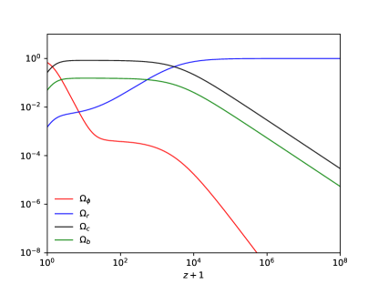
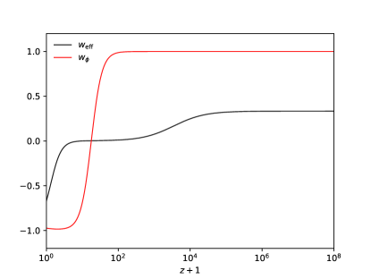
Figure 1: (Left panel) Evolution of $\Omega_{\phi}$, $\Omega_{r}$, $\Omega_{c}$, $\Omega_{b}$ versus $z+1$ ($z$ is the redshift) for $Q=-0.04$, $\lambda=0.5$, and $\beta=0.4$ with today’s density parameters $\Omega_{c0}=0.25$, $\Omega_{b0}=0.05$, and $\Omega_{r0}=1.0\times 10^{-4}$. (Right panel) Evolution of the effective equation of state $w_{\rm eff}$ and the scalar-field equation of state $w_{\phi}$ for the same model parameters and initial conditions as those used in the left.

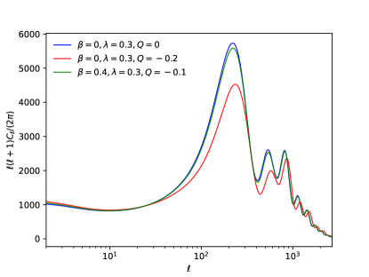
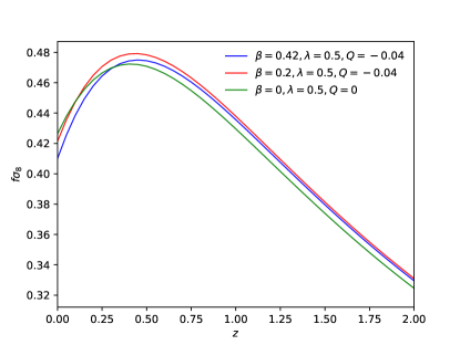
Figure 2: (Left panel) Theoretical CMB temperature anisotropies versus the multipole $\ell$ for three different model parameter sets: (i) $\beta=0$, $\lambda=0.3$, $Q=0$, (ii) $\beta=0$, $\lambda=0.3$, $Q=-0.2$, and (iii) $\beta=0.4$, $\lambda=0.3$, $Q=-0.1$. (Right panel) Evolution of $f\sigma_{8}$ versus the redshift $z$ for three different cases: (i) $\beta=0.42$, $\lambda=0.5$, $Q=-0.04$, (ii) $\beta=0.2$, $\lambda=0.5$, $Q=-0.04$, and (iii) $\beta=0$, $\lambda=0.5$, $Q=0$.

In Fig. 1, we plot the density parameters $\Omega_{\phi}$, $\Omega_{r}$, $\Omega_{c}$, $\Omega_{b}$ (left panel) and $w_{\rm eff}$, $w_{\phi}$ (right panel) for the model parameters $Q=-0.04$, $\lambda=0.5$, and $\beta=0.4$. We observe that the solution temporally approaches the $\phi$MDE characterized by $\Omega_{\phi}=w_{\rm eff}=2Q^{2}/[3(1+2\beta)]$, which is a distinguished feature compared to the $\Lambda$CDM model. The $\phi$MDE is followed by the epoch of cosmic acceleration ($w_{\rm eff}<-1/3$) driven by the fixed point (C).

In left panel of Fig. 2, we show the CMB angular power spectra of temperature anisotropies for several different values of $Q$ and $\beta$, with $\lambda=0.3$. Compared to the uncoupled quintessence, there are two main effects on CMB induced mostly by the coupling $Q$. The first is the shift of acoustic peaks toward larger multipoles $\ell$. The multiple $\ell_{A}$ corresponding to the sound horizon $r_{s*}$ at decoupling (redshift $z_{*}$) is given by

$$\ell_{A}=\pi\frac{D_{A}(z_{*})}{r_{s*}}\,,$$ (80)

where

$$D_{A}(z_{*})=\int_{0}^{z_{*}}\frac{1}{H(z)}{\rm d}z$$ (81)

is the comoving angular diameter distance, and

$$r_{s*}=\frac{1}{\sqrt{3}}\int_{0}^{a_{*}}\frac{{\rm d}a}{\sqrt{1+R_{s}(a)}\,a^{2}H(a)}\,,$$ (82)

with $R_{s}(a)=(3\Omega_{b0}/4\Omega_{\gamma 0})a$ and $a_{*}=(1+z_{*})^{-1}$ Hu and Sugiyama (1995); Amendola and Tsujikawa (2015). Here, $\Omega_{b0}$ and $\Omega_{\gamma 0}$ are today’s density parameters of baryons and photons, respectively. In our model, there is the $\phi$MDE in which the CDM density grows faster toward the higher redshift ($\rho_{c}\propto(1+z)^{3+2Q^{2}/(1+2\beta)}$) in comparison to the uncoupled case ($Q=0$). Moreover, the scalar-field density $\rho_{\phi}$ scales in the same manner as $\rho_{c}$ during the $\phi$MDE. These properties lead to the larger Hubble expansion rate before the decoupling epoch, so that the sound horizon (82) gets smaller in comparison to the uncoupled case.

The coupling $Q$ can increase the value of $H(z)$ from the end of the $\phi$MDE toward the decoupling epoch $z=z_{*}$, which results in the decrease of $D_{A}(z_{*})$. However, for fixed $H_{0}$, the increase of $1/r_{s*}$ induced by the same coupling typically overwhelms the reduction of $D_{A}(z_{*})$ in the estimation of $\ell_{A}$ in Eq. (80). For the model parameters $Q=0$ with $\beta=0$ and $\lambda=0.5$, we obtain the numerical values $D_{A}(z_{*})=13.84$ Gpc and $r_{s*}=144.40$ Mpc. If we change the coupling $Q$ to $-0.2$, the two distances change to $D_{A}(z_{*})=12.95$ Gpc and $r_{s*}=127.20$ Mpc, respectively. Clearly, the reduction of $r_{s*}$ induced by the coupling $Q$ is stronger than the decrease of $D_{A}(z_{*})$, which leads to the increase of $\ell_{A}$ from 301.17 (for $Q=0$) to 319.85 (for $Q=-0.2$). Hence the larger coupling $|Q|$ leads to the shift of CMB acoustic peaks toward smaller scales. This effect tends to be significant especially for $|Q|\gtrsim 0.1$. We note that the positive coupling $\beta$ works to suppress the factor $2Q^{2}/(1+2\beta)$ in the $(1+z)$-dependent power of $\rho_{c}$ during the $\phi$MDE. In comparison to the case $\beta=0$, we need to choose larger values of $|Q|$ to have the shift of acoustic peaks toward smaller scales.

The second effect of the coupling $Q$ on the CMB temperature spectrum is the suppressed amplitude of acoustic peaks. The existence of the $\phi$MDE gives rise to the larger CDM density $\rho_{c}$ at decoupling, while the baryon density $\rho_{b}$ is hardly affected. Then, the coupling $Q$ gives rise to a smaller ratio $\rho_{b}/\rho_{c}$ around $z=z_{*}$. For $Q=0$ with $\beta=0$ and $\lambda=0.5$, we obtain the numerical value $\rho_{b}/\rho_{c}=0.186$, while, for $Q=-0.2$ with the same values of $\beta$ and $\lambda$, this ratio decreases to $\rho_{b}/\rho_{c}=0.116$. This is the main reason for the reduction of the height of CMB acoustic peaks seen in Fig. 2. We note that, in the MCMC analysis performed in Sec. V, the best-fit value of today’s density parameter $\Omega_{c0}$ is slightly smaller than the one in the $\Lambda$CDM model. However, for $Q\neq 0$, the increase of $\rho_{c}$ toward the past during the $\phi$MDE results in the larger CDM density at decoupling in comparison to the uncoupled case, suppressing the early ISW contribution around the first acoustic peak.

In the right panel of Fig. 2, we show the evolution of $f\sigma_{8}$ for several different model parameters, where $f=\dot{\delta}_{m}/(H\delta_{m})$ is the growth rate of matter density contrast (incorporating both CDM and baryons) and $\sigma_{8}$ is the amplitude of matter over-density at the comoving $8h^{-1}$ Mpc scale ($h$ is the normalized Hubble constant $H_{0}=100\,h$ km/s/Mpc). We find that the large coupling $\beta$ induces the suppression for the growth rate of matter perturbations at low redshifts. This is also the case even in the presence of the coupling $Q$ of order $-0.01$. This result is consistent with the analytic estimation for the growth of perturbations discussed in Sec. III.

V Results and discussion

We are now going to place observational constraints on our model by using the MCMC likelihood CosmoMC Lewis and Bridle (2002). In our analysis, we will exploit the following data sets.

(i) The CMB data containing TT, TE, EE+lowE from Planck 2018 Aghanim et al. (2020c), and the large-scale structure data from the 12-th data release of SDSS Alam et al. (2015).

(ii) The Phantheon supernovae samples containing $1048$ type Ia supernovae magnitudes with redshift in the range of $0.01<z<2.3$ Scolnic et al. (2018), which are commonly used to constrain the property of late-time cosmic acceleration.

(iii) The 1-st year DES results Abbott et al. (2018b), which are the combined analyses of galaxy clustering and weak gravitational lensing.

We stop the calculations when the Gelman-Rubin statistic $R-1\sim 0.01$ is reached.

In Fig. 3 and Table 1, we present the results of observational constraints on our model parameters.

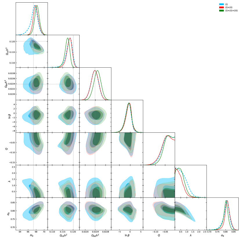
Figure 3: Triangle plot for the 1-dimensional marginalized distributions on individual parameters and the 1$\sigma$ and 2$\sigma$ 2-dimensional contours. The blue dashed lines represent constraints by the Planck 2018 Planck Collaboration (2020) and 12-th SDSS data sets, which we call (i). The red and green solid lines correspond to constraints when the data sets (ii) and (ii)+(iii) are combined with (i), respectively.

Table 1: Priors, mean values, best-fit values and 1$\sigma$ errors of the model parameters $\ln\beta$, $\lambda$, $Q$ and cosmological parameters $H_{0}$, $\Omega_{c0}h^{2},\Omega_{b0}h^{2}$, $\sigma_{8}$, where $\Omega_{c0}$ and $\Omega_{b0}$ are today’s density parameters of CDM and baryons respectively. The third, fourth, and fifth columns correspond to the constraints derived by the data sets (i), (i)$+$(ii), and (i)$+$(ii)$+$(iii), respectively.

Parameters	Priors	mean (best fit) (i)	mean (best fit) (i)+(ii)	mean (best fit) (i)+(ii)+(iii)
$H_{0}$ [km/s/Mpc]	$[20,100]$	$67.44(67.26)^{+1.01}_{-0.69}$	$67.93(67.66)^{+0.58}_{-0.68}$	$68.22(68.41)^{+0.58}_{-0.61}$
$\Omega_{c0}h^{2}$	$[0.001,0.99]$	$0.11802(0.11958)^{+0.0018}_{-0.0010}$	$0.11819(0.11904)^{+0.0014}_{-0.0010}$	$0.11712(0.11580)^{+0.0013}_{-0.0009}$
$\Omega_{b0}h^{2}$	$[0.005,0.1]$	$0.02237(0.02237)^{+0.00014}_{-0.00014}$	$0.02237(0.02238)^{+0.00015}_{-0.00014}$	$0.02247(0.02248)^{+0.00014}_{-0.00013}$
$\ln\beta$	*	$-1.0131(-0.1997)^{+1.5750}_{-1.1754}$	$-0.7919(-1.5209)^{+1.5452}_{-1.1593}$	$-0.8754(-2.6179)^{+1.5652}_{-1.3223}$
$\lambda$	$[0.1,\infty]$	$0.6028(0.4083)^{+0.1668}_{-0.5928}$	$0.4235(0.2467)^{+0.1057}_{-0.4088}$	$0.4988(0.5269)^{+0.1419}_{-0.4676}$
$Q$	$[-\infty,0]$	$-0.0396(-0.0072)^{+0.0396}_{-0.0108}$	$-0.0422(-0.0096)^{+0.0408}_{-0.0125}$	$-0.0355(-0.0396)^{+0.0355}_{-0.0097}$
$\sigma_{8}$	*	$0.8031(0.8057)^{+0.0231}_{-0.0148}$	$0.8105(0.8058)^{+0.0169}_{-0.0148}$	$0.7996(0.8084)^{+0.0174}_{-0.0120}$

First, let us discuss constraints on the parameter $\beta$. In Table 1, the bounds on $\beta$ (68 % CL) constrained by different data sets are presented in terms of the log prior. From the joint analysis based on the data sets (i)$+$(ii)$+$(iii), this bound translates to

$$\beta=0.417^{+1.592}_{-0.307}\qquad(68\,\%\,{\rm CL})\,,$$ (83)

where 0.417 is the mean value. Since $\beta$ is constrained to be larger than 0.11 at 1$\sigma$, there is an interesting observational signature of the momentum exchange between DE and DM. Even with the analysis of the data set (i) or with the data sets (i)$+$(ii), the $1\sigma$ lower limits on $\beta$ are close to the value 0.1. Hence the Planck CMB data combined with the SDSS data already show the signature of the momentum transfer. We note that this result is consistent with the likelihood analysis of Refs. Pourtsidou and Tram (2016); Linton et al. (2018); Chamings et al. (2020); Linton et al. (2022) performed for the model $Q=0$, where the joint analysis based on the CMB and galaxy clustering data favour nonvanishing values of $\beta$.

With the data sets (i)$+$(ii)$+$(iii), we also obtain the following 2$\sigma$ bound

$$0.014<\beta<10.756\qquad(95\,\%\,{\rm CL})\,.$$ (84)

Since the lower limit of $\beta$ is as small as $0.01$, this value is not significantly distinguished from $\beta=0$. This means that the evidence for the momentum transfer can be confirmed at 68 % CL, but not firmly at 95 % CL, with the current observational data. We note that the mean value of $\sigma_{8}$ constrained by the data sets (i)$+$(ii)$+$(iii) is 0.7996, which is smaller than the Planck 2018 bound $\sigma_{8}=0.8111\pm 0.0060$ Aghanim et al. (2020a) derived for the $\Lambda$CDM model. Thus, in our model, the $\sigma_{8}$ tension between the CMB and other measurements is alleviated by the momentum transfer. This property is mostly attributed to the fact that the growth rate of $\delta_{c}$ at low redshifts is suppressed by the positive coupling $\beta$.

The other coupling constant $Q$, which mediates the energy transfer between DE and DM, is constrained to be

$$Q=-0.0355^{+0.0355}_{-0.0097}\qquad(68\,\%\,{\rm CL})\,,$$ (85)

where $-0.0355$ is the mean value. As we see in Fig. 3, the analysis based on the data sets (i) $+$ (ii) gives rise to a peak in the 1-dimensional probability distribution of $Q$ around $-0.04$. This property also holds by adding the data set (iii). Since the vanishing coupling ($Q=0$) is within the $1\sigma$ contour, we do not have strong observational evidence that the nonvanishing value of $Q$ is favored over the $Q=0$ case. However, it is interesting to note that the current data give rise to the probability distribution of $Q$ with a peak at $Q<0$.

In Refs. Pettorino (2013); Ade et al. (2016); Gómez-Valent et al. (2020), the couplings $|Q|$ slightly smaller than the mean value of (85) were obtained by the MCMC analysis with several data sets for the coupled dark energy model with $\beta=0$. In our model, we have $\Omega_{\phi}=w_{\rm eff}=2Q^{2}/[3(1+2\beta)]$ during the $\phi$MDE, so both $\Omega_{\phi}$ and $w_{\rm eff}$ are suppressed by the positive coupling $\beta$. This allows the larger values of $|Q|$ in comparison to the case $\beta=0$. Still, the coupling $|Q|$ exceeding the order $0.1$ is forbidden from the data because of the significant changes of heights and positions in CMB acoustic peaks (see Fig. 2).

The parameter $\lambda$ is related to the slope of the scalar-field potential. To realize the DE equation of state closer to $-1$ at late times, we require that $\lambda$ can not be significantly away from 0. From the MCMC analysis with the data sets (i)$+$(ii)$+$(iii), we obtain the upper limit

$$\lambda<0.641\qquad(68\,\%\,{\rm CL})\,.$$ (86)

We also remark that, for larger $\lambda$, the distance to the CMB last scattering surface is reduced. To compensate this property, we require smaller values of $H_{0}$. This explains the tendency for blue contours seen in the $\lambda$-$H_{0}$ plane. Thus, the smaller values of $\lambda$ are favored from the viewpoint of increasing $H_{0}$.

In Fig. 3, we find that today’s CDM density parameter $\Omega_{c0}$ is constrained to be smaller than the Planck 2018 bound $\Omega_{c0}h^{2}=0.120\pm 0.001$ derived for the $\Lambda$CDM model Aghanim et al. (2020a). In spite of this decrease of $\Omega_{c0}$, the CDM density evolves as $\rho_{c}\propto(1+z)^{3+2Q^{2}/(1+2\beta)}$ during the $\phi$MDE and hence $\Omega_{c}$ at decoupling can be increased by the nonvanishing coupling $Q$. We note that today’s baryon density parameter $\Omega_{b0}$ is only slightly larger than the Planck 2018 bound $\Omega_{b0}=0.0224\pm 0.0001$ (see Fig. 3). Then, the nonvanishing coupling $Q$ hardly modifies the value of $\Omega_{b}$ at $z=z_{*}$ in comparison to the case $Q=0$. Since the ratio $\Omega_{b}/\Omega_{c}$ at decoupling is decreased by the coupling $|Q|$ larger than the order $0.01$, this suppresses the height of CMB acoustic peaks. The MCMC analysis with the CMB data alone already places the bound $|Q|<0.1$ at 95 % CL.

As we discussed in Sec. IV, the nonvanishing coupling $Q$ reduces the sound horizon $r_{s*}$ at $z=z_{*}$. This leads to the shift of CMB acoustic peaks toward smaller scales. To keep the position of the multipole $\ell_{A}$ corresponding to the sound horizon, we require that the comoving angular diameter distance $D_{A}(z_{*})$ appearing in the numerator of Eq. (80) should be also reduced. We can express Eq. (81) as $D_{A}(z_{*})=H_{0}^{-1}\int_{0}^{z_{*}}E^{-1}(z){\rm d}z$, where $E(z)=H(z)/H_{0}$. In the $\Lambda$CDM model we have $E(z)=[\Omega_{m0}(1+z)^{3}+\Omega_{\Lambda}+\Omega_{r0}(1+z)^{4}]^{1/2}$, where $\Omega_{m0}=\Omega_{c0}+\Omega_{b0}$. In our model, the CDM density parameter during the $\phi$MDE has the dependence $\Omega_{c0}(1+z)^{3+2Q^{2}/(1+2\beta)}$ instead of $\Omega_{c0}(1+z)^{3}$, together with the scaling behavior of $\rho_{\phi}$ with $\rho_{c}$. Then, the coupling $Q$ leads to the increase of $E(z)$ from the end of $\phi$MDE to the decoupling epoch, so that the integral $\int_{0}^{z_{*}}E^{-1}(z){\rm d}z$ is decreased. This property is different from the early DE scenario of Ref. Poulin et al. (2019), where the energy density of early DE quickly decays after the recombination epoch.

In our model, increasing the value of $H_{0}$ also reduces $D_{A}(z_{*})$, so it can compensate the reduction of $r_{s*}$. However, the integral $\int_{0}^{z_{*}}E^{-1}(z){\rm d}z$ is already decreased at some extent by the existence of the $\phi$MDE. In this sense, there is the limitation for realizing $H_{0}$ significantly larger than the value obtained for $Q=0$. The observational constraint on $H_{0}$ derived by the data set (i) for the model with $Q=0$ is consistent with the Planck 2018 bound $H_{0}=67.27\pm 0.60$ km/s/Mpc. In the presence of the negative coupling $Q$, the likelihood region in the $Q$-$H_{0}$ plane shown in Fig. 3 shifts toward larger values of $H_{0}$. With the full data sets (i)$+$(ii)$+$(iii), the Hubble constant is constrained to be

$$H_{0}=68.22^{+0.58}_{-0.61}~{}{\rm km/s/Mpc}\qquad(68\,\%\,{\rm CL})\,,$$ (87)

whose mean value is larger than the one derived for the $\Lambda$CDM model with the Planck 2018 data alone. However, it is not possible to reach the region $H_{0}>70$ km/s/Mpc due to the limitation of reducing $D_{A}(z_{*})$ by increasing the value of $H_{0}$. We also carried out the MCMC analysis for the $\Lambda$CDM model and obtained the bound $H_{0}=68.19^{+0.37}_{-0.38}~{}{\rm km/s/Mpc}$ with the full data sets (i)$+$(ii)$+$(iii). The $1\sigma$ upper limit of the constraint (87) is only slightly larger than that of the $\Lambda$CDM bound. Hence the Hubble tension problem between the Planck 2018 data and those constrained by the direct measurements of $H_{0}$ still persists in our coupled DE scenario.

Albeit the difficulty of resolving the Hubble tension problem, the fact that the probability distribution of $Q$ has a peak around $-0.04$ is an interesting property of our model. Moreover, there are observational signatures of the momentum transfer with $\beta>0$ between DE and DM at 68 % CL. The coupling $\beta$ can alleviate the $\sigma_{8}$ tension without spoiling the existence of the $\phi$MDE.

VI Conclusions

In this paper, we put observational constraints on an interacting model of DE and DM given by the action (2). Since our model has a concrete Lagrangian, the background and perturbation equations of motion are unambiguously fixed by the variational principle. This is not the case for many coupled DE-DM models studied in the literature, in which the interacting terms are added to the background equations by hands. In our model, the DE scalar field $\phi$ and the CDM fluid mediate both energy and momentum transfers, whose coupling strengths are characterized by the constants $Q$ and $\beta$, respectively. We considered an exponential potential $V(\phi)=V_{0}e^{-\lambda\phi/M_{\rm Pl}}$ of the scalar field to derive late-time cosmic acceleration, but the different choice of quintessence potentials should not affect the observational constraints on $Q$ and $\beta$ significantly.

The coupling $Q$ can give rise to the $\phi$MDE during which the scalar-field density parameter $\Omega_{\phi}$ and the effective equation of state $w_{\rm eff}$ are nonvanishing constants, such that $\Omega_{\phi}=w_{\rm eff}=2Q^{2}/[3(1+2\beta)]$. In this epoch, the CDM density grows as $\rho_{c}\propto(1+z)^{3+2Q^{2}/(1+2\beta)}$ toward the past and hence the value of $\rho_{c}$ at CMB decoupling can be increased by the coupling $Q$. Since this enhances the Hubble expansion rate in the past, the sound horizon $r_{s*}$ at decoupling (redshift $z_{*}$) gets smaller. Moreover, the ratio between the baryon and CDM densities, $\rho_{b}/\rho_{c}$, is suppressed at $z=z_{*}$ due to the increase of $\rho_{c}$ induced by the presence of the $\phi$MDE. These modifications shift the positions and heights of acoustic peaks of CMB temperature anisotropies, so that the coupling $Q$ can be tightly constrained from the CMB data.

The effect of momentum transfers on the dynamics of perturbations mostly manifests itself for the evolution of CDM density contrast $\delta_{c}$ at low redshifts. For $\beta>0$, the growth of $\delta_{c}$ is suppressed due to the decrease of an effective gravitational coupling $G_{\rm eff}$ on scales relevant to the galaxy clustering. The coupling $Q$ enhances the value of $G_{\rm eff}$ through the energy transfer between DE and DM. However, the reduction of $G_{\rm eff}$ induced by positive $\beta$ typically overwhelms the increase of $G_{\rm eff}$ for the redshift $z\lesssim 1$. Hence the growth rate of CDM perturbations is suppressed in comparison to the $\Lambda$CDM model.

We carried out the MCMC analysis for our model by using the observational data of Planck 2018 Aghanim et al. (2020c), 12-th SDSS, Phantheon supernovae samples, and 1-year DES. The coupling $\beta$ is constrained to be in the range $\beta=0.417^{+1.592}_{-0.307}$ (68 % CL) by using all the data sets. Since the $\beta=0$ case is outside the $1\sigma$ observational contour, there is an interesting observational signature of the momentum transfer between DE and DM. This is an outcome of the suppressed growth of $\delta_{c}$ at low redshifts, thereby easing the $\sigma_{8}$ tension. Indeed, we found that the mean value of $\sigma_{8}$ constrained by the full data is $0.7996$, which is smaller than the best-fit value $0.8111$ derived for the $\Lambda$CDM model with the Planck data alone.

For the coupling characterizing the energy transfer, we obtained the bound $Q=-0.0355^{+0.0355}_{-0.0097}$ (68 % CL) by the analysis with full data sets. While the $Q=0$ case is within the $1\sigma$ observational contour, there is a peak for the probability distribution of the coupling at a negative value of $Q$. This result is consistent with the likelihood analysis performed for the model with $\beta=0$ Pettorino (2013); Ade et al. (2016); Gómez-Valent et al. (2020), but now the constrained values of $|Q|$ get larger. This increase of $|Q|$ is mostly attributed to the fact that the effective equation of state during the $\phi$MDE is modified to $w_{\rm eff}=2Q^{2}/[3(1+2\beta)]$ through the coupling $\beta$. In comparison to the momentum transfer, we have not yet detected significant observational signatures of the energy transfer, but the future high-precision data will clarify this issue.

The presence of the coupling $Q$ reduces the sound horizon $r_{s*}$ at decoupling, thereby increasing the multipole $\ell_{A}$ defined in Eq. (80). To keep the position of CMB acoustic peaks, we require that the comoving angular diameter distance $D_{A}(z_{*})$ from $z=0$ to $z=z_{*}$ decreases. During the $\phi$MDE, the Hubble expansion rate increases due to the enhancement of $\rho_{c}$ induced by the energy transfer. Since this leads to the decrease of $D_{A}(z_{*})$, the further reduction of $D_{A}(z_{*})$ by the choice of larger values of $H_{0}$ is quite limited in our model. From the MCMC analysis of full data sets we obtained the bound $H_{0}=68.22^{+0.58}_{-0.61}~{}{\rm km/s/Mpc}$, whose mean value is larger than the one derived for the $\Lambda$CDM model with the Planck 2018 data alone. However, the Hubble constant $H_{0}$ does not exceed the value $70~{}{\rm km/s/Mpc}$, so the Hubble tension problem is not completely resolved in our scenario.

It is still encouraging that the current data support signatures of the interaction between DE and DM. We expect that upcoming observational data like those from the Euclid satellite will place further tight constraints on the couplings $\beta$ and $Q$. Along with the $H_{0}$ tension problem, we hope that we will be able to approach the origins of DE and DM and their possible interactions in the foreseeable future.

References

- Jungman et al. (1996) G. Jungman, M. Kamionkowski, and K. Griest, Phys. Rept. 267, 195 (1996), arXiv:hep-ph/9506380 .
- Bertone et al. (2005) G. Bertone, D. Hooper, and J. Silk, Phys. Rept. 405, 279 (2005), arXiv:hep-ph/0404175 .
- Peebles and Ratra (2003) P. J. E. Peebles and B. Ratra, Rev. Mod. Phys. 75, 559 (2003), arXiv:astro-ph/0207347 .
- Copeland et al. (2006) E. J. Copeland, M. Sami, and S. Tsujikawa, Int. J. Mod. Phys. D 15, 1753 (2006), arXiv:hep-th/0603057 .
- Silvestri and Trodden (2009) A. Silvestri and M. Trodden, Rept. Prog. Phys. 72, 096901 (2009), arXiv:0904.0024 [astro-ph.CO] .
- Kase and Tsujikawa (2019) R. Kase and S. Tsujikawa, Int. J. Mod. Phys. D 28, 1942005 (2019), arXiv:1809.08735 [gr-qc] .
- Ezquiaga and Zumalacárregui (2018) J. M. Ezquiaga and M. Zumalacárregui, Front. Astron. Space Sci. 5, 44 (2018), arXiv:1807.09241 [astro-ph.CO] .
- Weinberg (1989) S. Weinberg, Rev. Mod. Phys. 61, 1 (1989).
- Sahni and Starobinsky (2000) V. Sahni and A. A. Starobinsky, Int. J. Mod. Phys. D 9, 373 (2000), arXiv:astro-ph/9904398 .
- Padmanabhan (2003) T. Padmanabhan, Phys. Rept. 380, 235 (2003), arXiv:hep-th/0212290 .
- Carroll (2001) S. M. Carroll, Living Rev. Rel. 4, 1 (2001), arXiv:astro-ph/0004075 .
- Martin (2012) J. Martin, Comptes Rendus Physique 13, 566 (2012), arXiv:1205.3365 [astro-ph.CO] .
- Padilla (2015) A. Padilla, arXiv:1502.05296 [hep-th] .
- De Felice and Tsujikawa (2010) A. De Felice and S. Tsujikawa, Living Rev. Rel. 13, 3 (2010), arXiv:1002.4928 [gr-qc] .
- Clifton et al. (2012) T. Clifton, P. G. Ferreira, A. Padilla, and C. Skordis, Phys. Rept. 513, 1 (2012), arXiv:1106.2476 [astro-ph.CO] .
- Joyce et al. (2015) A. Joyce, B. Jain, J. Khoury, and M. Trodden, Phys. Rept. 568, 1 (2015), arXiv:1407.0059 [astro-ph.CO] .
- Koyama (2016) K. Koyama, Rept. Prog. Phys. 79, 046902 (2016), arXiv:1504.04623 [astro-ph.CO] .
- Ishak (2019) M. Ishak, Living Rev. Rel. 22, 1 (2019), arXiv:1806.10122 [astro-ph.CO] .
- Heisenberg (2019) L. Heisenberg, Phys. Rept. 796, 1 (2019), arXiv:1807.01725 [gr-qc] .
- Fujii (1982) Y. Fujii, Phys. Rev. D 26, 2580 (1982).
- Ford (1987) L. H. Ford, Phys. Rev. D 35, 2339 (1987).
- Ratra and Peebles (1988) B. Ratra and P. J. E. Peebles, Phys. Rev. D 37, 3406 (1988).
- Wetterich (1988) C. Wetterich, Nucl. Phys. B 302, 668 (1988), arXiv:1711.03844 [hep-th] .
- Chiba et al. (1997) T. Chiba, N. Sugiyama, and T. Nakamura, Mon. Not. Roy. Astron. Soc. 289, L5 (1997), arXiv:astro-ph/9704199 .
- Ferreira and Joyce (1997) P. G. Ferreira and M. Joyce, Phys. Rev. Lett. 79, 4740 (1997), arXiv:astro-ph/9707286 .
- Caldwell et al. (1998) R. R. Caldwell, R. Dave, and P. J. Steinhardt, Phys. Rev. Lett. 80, 1582 (1998), arXiv:astro-ph/9708069 .
- Zlatev et al. (1999) I. Zlatev, L.-M. Wang, and P. J. Steinhardt, Phys. Rev. Lett. 82, 896 (1999), arXiv:astro-ph/9807002 .
- Chiba et al. (2013) T. Chiba, A. De Felice, and S. Tsujikawa, Phys. Rev. D 87, 083505 (2013), arXiv:1210.3859 [astro-ph.CO] .
- Tsujikawa (2013) S. Tsujikawa, Class. Quant. Grav. 30, 214003 (2013), arXiv:1304.1961 [gr-qc] .
- Durrive et al. (2018) J.-B. Durrive, J. Ooba, K. Ichiki, and N. Sugiyama, Phys. Rev. D 97, 043503 (2018), arXiv:1801.09446 [astro-ph.CO] .
- Aghanim et al. (2020a) N. Aghanim et al. (Planck), Astron. Astrophys. 641, A6 (2020a), [Erratum: Astron.Astrophys. 652, C4 (2021)], arXiv:1807.06209 [astro-ph.CO] .
- Akrami et al. (2019) Y. Akrami, R. Kallosh, A. Linde, and V. Vardanyan, Fortsch. Phys. 67, 1800075 (2019), arXiv:1808.09440 [hep-th] .
- Heymans et al. (2012) C. Heymans et al., Mon. Not. Roy. Astron. Soc. 427, 146 (2012), arXiv:1210.0032 [astro-ph.CO] .
- Hildebrandt et al. (2017) H. Hildebrandt et al., Mon. Not. Roy. Astron. Soc. 465, 1454 (2017), arXiv:1606.05338 [astro-ph.CO] .
- Abbott et al. (2018a) T. Abbott et al. (DES), Phys. Rev. D 98, 043526 (2018a), arXiv:1708.01530 [astro-ph.CO] .
- Samushia et al. (2014) L. Samushia et al., Mon. Not. Roy. Astron. Soc. 439, 3504 (2014), arXiv:1312.4899 [astro-ph.CO] .
- Macaulay et al. (2013) E. Macaulay, I. K. Wehus, and H. K. Eriksen, Phys. Rev. Lett. 111, 161301 (2013), arXiv:1303.6583 [astro-ph.CO] .
- Aghanim et al. (2020b) N. Aghanim et al. (Planck), Astron. Astrophys. 641, A6 (2020b), arXiv:1807.06209 [astro-ph.CO] .
- Riess et al. (2018) A. G. Riess et al., Astrophys. J. 855, 136 (2018), arXiv:1801.01120 [astro-ph.SR] .
- Wong et al. (2020) K. C. Wong et al., Mon. Not. Roy. Astron. Soc. 498, 1420 (2020), arXiv:1907.04869 [astro-ph.CO] .
- Riess et al. (2021) A. G. Riess, S. Casertano, W. Yuan, J. B. Bowers, L. Macri, J. C. Zinn, and D. Scolnic, Astrophys. J. Lett. 908, L6 (2021), arXiv:2012.08534 [astro-ph.CO] .
- Verde et al. (2019) L. Verde, T. Treu, and A. Riess, Nature Astron. 3, 891 (2019), arXiv:1907.10625 [astro-ph.CO] .
- Di Valentino et al. (2021) E. Di Valentino, O. Mena, S. Pan, L. Visinelli, W. Yang, A. Melchiorri, D. F. Mota, A. G. Riess, and J. Silk, arXiv:2103.01183 [astro-ph.CO] .
- Perivolaropoulos and Skara (2021) L. Perivolaropoulos and F. Skara, arXiv:2105.05208 [astro-ph.CO] .
- Freedman (2021) W. L. Freedman, arXiv:2106.15656 [astro-ph.CO] .
- Wetterich (1995) C. Wetterich, Astron. Astrophys. 301, 321 (1995), arXiv:hep-th/9408025 .
- Amendola (2000) L. Amendola, Phys. Rev. D 62, 043511 (2000), arXiv:astro-ph/9908023 .
- Frusciante et al. (2019) N. Frusciante, R. Kase, K. Koyama, S. Tsujikawa, and D. Vernieri, Phys. Lett. B 790, 167 (2019), arXiv:1812.05204 [gr-qc] .
- Kase and Tsujikawa (2020a) R. Kase and S. Tsujikawa, Phys. Rev. D 101, 063511 (2020a), arXiv:1910.02699 [gr-qc] .
- Brans and Dicke (1961) C. Brans and R. H. Dicke, Phys. Rev. 124, 925 (1961).
- Amendola (1999) L. Amendola, Phys. Rev. D 60, 043501 (1999), arXiv:astro-ph/9904120 .
- Khoury and Weltman (2004) J. Khoury and A. Weltman, Phys. Rev. D 69, 044026 (2004), arXiv:astro-ph/0309411 .
- Tsujikawa et al. (2008) S. Tsujikawa, K. Uddin, S. Mizuno, R. Tavakol, and J. Yokoyama, Phys. Rev. D 77, 103009 (2008), arXiv:0803.1106 [astro-ph] .
- Pettorino (2013) V. Pettorino, Phys. Rev. D 88, 063519 (2013), arXiv:1305.7457 [astro-ph.CO] .
- Ade et al. (2016) P. A. R. Ade et al. (Planck), Astron. Astrophys. 594, A14 (2016), arXiv:1502.01590 [astro-ph.CO] .
- Gómez-Valent et al. (2020) A. Gómez-Valent, V. Pettorino, and L. Amendola, Phys. Rev. D 101, 123513 (2020), arXiv:2004.00610 [astro-ph.CO] .
- Amendola (2004) L. Amendola, Phys. Rev. D 69, 103524 (2004), arXiv:astro-ph/0311175 .
- Tsujikawa (2007) S. Tsujikawa, Phys. Rev. D 76, 023514 (2007), arXiv:0705.1032 [astro-ph] .
- Pourtsidou et al. (2013) A. Pourtsidou, C. Skordis, and E. Copeland, Phys. Rev. D 88, 083505 (2013), arXiv:1307.0458 [astro-ph.CO] .
- Boehmer et al. (2015) C. G. Boehmer, N. Tamanini, and M. Wright, Phys. Rev. D 91, 123003 (2015), arXiv:1502.04030 [gr-qc] .
- Skordis et al. (2015) C. Skordis, A. Pourtsidou, and E. Copeland, Phys. Rev. D 91, 083537 (2015), arXiv:1502.07297 [astro-ph.CO] .
- Koivisto et al. (2015) T. S. Koivisto, E. N. Saridakis, and N. Tamanini, JCAP 09, 047 (2015), arXiv:1505.07556 [astro-ph.CO] .
- Pourtsidou and Tram (2016) A. Pourtsidou and T. Tram, Phys. Rev. D 94, 043518 (2016), arXiv:1604.04222 [astro-ph.CO] .
- Dutta et al. (2017) J. Dutta, W. Khyllep, and N. Tamanini, Phys. Rev. D 95, 023515 (2017), arXiv:1701.00744 [gr-qc] .
- Linton et al. (2018) M. S. Linton, A. Pourtsidou, R. Crittenden, and R. Maartens, JCAP 04, 043 (2018), arXiv:1711.05196 [astro-ph.CO] .
- Kase and Tsujikawa (2020b) R. Kase and S. Tsujikawa, Phys. Lett. B 804, 135400 (2020b), arXiv:1911.02179 [gr-qc] .
- Chamings et al. (2020) F. N. Chamings, A. Avgoustidis, E. J. Copeland, A. M. Green, and A. Pourtsidou, Phys. Rev. D 101, 043531 (2020), arXiv:1912.09858 [astro-ph.CO] .
- Amendola and Tsujikawa (2020) L. Amendola and S. Tsujikawa, JCAP 06, 020 (2020), arXiv:2003.02686 [gr-qc] .
- Kase and Tsujikawa (2020c) R. Kase and S. Tsujikawa, JCAP 11, 032 (2020c), arXiv:2005.13809 [gr-qc] .
- Linton et al. (2022) M. S. Linton, R. Crittenden, and A. Pourtsidou, JCAP 08, 075 (2022), arXiv:2107.03235 [astro-ph.CO] .
- Dalal et al. (2001) N. Dalal, K. Abazajian, E. E. Jenkins, and A. V. Manohar, Phys. Rev. Lett. 87, 141302 (2001), arXiv:astro-ph/0105317 .
- Zimdahl and Pavon (2001) W. Zimdahl and D. Pavon, Phys. Lett. B 521, 133 (2001), arXiv:astro-ph/0105479 .
- Chimento et al. (2003) L. P. Chimento, A. S. Jakubi, D. Pavon, and W. Zimdahl, Phys. Rev. D 67, 083513 (2003), arXiv:astro-ph/0303145 .
- Wang et al. (2005) B. Wang, Y.-g. Gong, and E. Abdalla, Phys. Lett. B 624, 141 (2005), arXiv:hep-th/0506069 .
- Amendola et al. (2007) L. Amendola, G. Camargo Campos, and R. Rosenfeld, Phys. Rev. D 75, 083506 (2007), arXiv:astro-ph/0610806 .
- Guo et al. (2007) Z.-K. Guo, N. Ohta, and S. Tsujikawa, Phys. Rev. D 76, 023508 (2007), arXiv:astro-ph/0702015 .
- Valiviita et al. (2008) J. Valiviita, E. Majerotto, and R. Maartens, JCAP 07, 020 (2008), arXiv:0804.0232 [astro-ph] .
- Salvatelli et al. (2014) V. Salvatelli, N. Said, M. Bruni, A. Melchiorri, and D. Wands, Phys. Rev. Lett. 113, 181301 (2014), arXiv:1406.7297 [astro-ph.CO] .
- Kumar and Nunes (2016) S. Kumar and R. C. Nunes, Phys. Rev. D 94, 123511 (2016), arXiv:1608.02454 [astro-ph.CO] .
- Di Valentino et al. (2017) E. Di Valentino, A. Melchiorri, and O. Mena, Phys. Rev. D 96, 043503 (2017), arXiv:1704.08342 [astro-ph.CO] .
- Yang et al. (2018) W. Yang, S. Pan, E. Di Valentino, R. C. Nunes, S. Vagnozzi, and D. F. Mota, JCAP 09, 019 (2018), arXiv:1805.08252 [astro-ph.CO] .
- Pan et al. (2019) S. Pan, W. Yang, E. Di Valentino, E. N. Saridakis, and S. Chakraborty, Phys. Rev. D 100, 103520 (2019), arXiv:1907.07540 [astro-ph.CO] .
- Di Valentino et al. (2020a) E. Di Valentino, A. Melchiorri, O. Mena, and S. Vagnozzi, Phys. Dark Univ. 30, 100666 (2020a), arXiv:1908.04281 [astro-ph.CO] .
- Di Valentino et al. (2020b) E. Di Valentino, A. Melchiorri, O. Mena, and S. Vagnozzi, Phys. Rev. D 101, 063502 (2020b), arXiv:1910.09853 [astro-ph.CO] .
- Salzano et al. (2021) V. Salzano et al., JCAP 09, 033 (2021), arXiv:2102.06417 [astro-ph.CO] .
- Poulin et al. (2023) V. Poulin, J. L. Bernal, E. D. Kovetz, and M. Kamionkowski, Phys. Rev. D 107, 123538 (2023), arXiv:2209.06217 [astro-ph.CO] .
- Asghari et al. (2019) M. Asghari, J. Beltrán Jiménez, S. Khosravi, and D. F. Mota, JCAP 04, 042 (2019), arXiv:1902.05532 [astro-ph.CO] .
- Beltrán Jiménez et al. (2020) J. Beltrán Jiménez, D. Bettoni, D. Figueruelo, and F. A. Teppa Pannia, JCAP 08, 020 (2020), arXiv:2004.14661 [astro-ph.CO] .
- Beltrán Jiménez et al. (2021a) J. Beltrán Jiménez, D. Bettoni, D. Figueruelo, F. A. Teppa Pannia, and S. Tsujikawa, JCAP 03, 085 (2021a), arXiv:2012.12204 [astro-ph.CO] .
- Beltrán Jiménez et al. (2021b) J. Beltrán Jiménez, D. Bettoni, D. Figueruelo, F. A. Teppa Pannia, and S. Tsujikawa, Phys. Rev. D 104, 103503 (2021b), arXiv:2106.11222 [astro-ph.CO] .
- De Felice et al. (2020) A. De Felice, S. Nakamura, and S. Tsujikawa, Phys. Rev. D 102, 063531 (2020), arXiv:2004.09384 [gr-qc] .
- Aghanim et al. (2020c) N. Aghanim et al. (Planck), Astron. Astrophys. 641, A5 (2020c), arXiv:1907.12875 [astro-ph.CO] .
- Alam et al. (2015) S. Alam et al. (SDSS-III), Astrophys. J. Suppl. 219, 12 (2015), arXiv:1501.00963 [astro-ph.IM] .
- Scolnic et al. (2018) D. M. Scolnic et al. (Pan-STARRS1), Astrophys. J. 859, 101 (2018), arXiv:1710.00845 [astro-ph.CO] .
- Abbott et al. (2018b) T. M. C. Abbott et al. (DES), Phys. Rev. D 98, 043526 (2018b), arXiv:1708.01530 [astro-ph.CO] .
- Schutz and Sorkin (1977) B. F. Schutz and R. Sorkin, Annals Phys. 107, 1 (1977).
- Brown (1993) J. Brown, Class. Quant. Grav. 10, 1579 (1993), arXiv:gr-qc/9304026 .
- De Felice et al. (2010) A. De Felice, J.-M. Gerard, and T. Suyama, Phys. Rev. D 81, 063527 (2010), arXiv:0908.3439 [gr-qc] .
- Lewis et al. (2000) A. Lewis, A. Challinor, and A. Lasenby, The Astrophysical Journal 538, 473 (2000).
- Ma and Bertschinger (1995) C.-P. Ma and E. Bertschinger, Astrophys. J. 455, 7 (1995), arXiv:astro-ph/9506072 .
- Hu and Sugiyama (1995) W. Hu and N. Sugiyama, Astrophys. J. 444, 489 (1995), arXiv:astro-ph/9407093 .
- Amendola and Tsujikawa (2015) L. Amendola and S. Tsujikawa, Dark Energy: Theory and Observations (Cambridge University Press, 2015).
- Lewis and Bridle (2002) A. Lewis and S. Bridle, Phys. Rev. D 66, 103511 (2002).
- Planck Collaboration (2020) Planck Collaboration, Astronomy & Astrophysics 641, A6 (2020).
- Poulin et al. (2019) V. Poulin, T. L. Smith, T. Karwal, and M. Kamionkowski, Phys. Rev. Lett. 122, 221301 (2019), arXiv:1811.04083 [astro-ph.CO] .