Provable Training for Graph Contrastive Learning

Abstract

Graph Contrastive Learning (GCL) has emerged as a popular training approach for learning node embeddings from augmented graphs without labels. Despite the key principle that maximizing the similarity between positive node pairs while minimizing it between negative node pairs is well established, some fundamental problems are still unclear. Considering the complex graph structure, are some nodes consistently well-trained and following this principle even with different graph augmentations? Or are there some nodes more likely to be untrained across graph augmentations and violate the principle? How to distinguish these nodes and further guide the training of GCL? To answer these questions, we first present experimental evidence showing that the training of GCL is indeed imbalanced across all nodes. To address this problem, we propose the metric "node compactness", which is the lower bound of how a node follows the GCL principle related to the range of augmentations. We further derive the form of node compactness theoretically through bound propagation, which can be integrated into binary cross-entropy as a regularization. To this end, we propose the PrOvable Training (POT) for GCL, which regularizes the training of GCL to encode node embeddings that follows the GCL principle better. Through extensive experiments on various benchmarks, POT consistently improves the existing GCL approaches, serving as a friendly plugin.

1 Introduction

Graph Neural Networks (GNNs) are successful in many graph-related applications, e.g., node classification [10, 20] and link prediction [33, 27]. Traditional GNNs follow a semi-supervised learning paradigm requiring task-specific high-quality labels, which are expensive to obtain [9]. To alleviate the dependence on labels, graph contrastive learning (GCL) is proposed and has received considerable attention recently [35, 31, 25, 21, 29]. As a typical graph self-supervised learning technique, GCL shows promising results on many downstream tasks [22, 30, 23].

The learning process of GCL usually consists of the following steps: generate two graph augmentations [35]; feed these augmented graphs into a graph encoder to learn the node embeddings, and then optimize the whole training process based on the InfoNCE principle [15, 35, 36], where the positive and negative node pairs are selected from the two augmentations. With this principle ("GCL principle" for short), GCL learns the node embeddings where the similarities between the positive node pairs are maximized while the similarities between the negative node pairs are minimized.

However, it is well known that the real-world graph structure is complex and different nodes may have different properties [1, 2, 11, 36]. When generating augmentations and training on the complex graph structure in GCL, it may be hard for all nodes to follow the GCL principle well enough. This naturally gives rise to the following questions: are some of the nodes always well-trained and following the principle of GCL given different graph augmentations? Or are there some nodes more likely not to be well trained and violate the principle? If so, it implies that each node should not be treated equally in the training process. Specifically, GCL should pay less attention to those well-trained nodes that already satisfy the InfoNCE principle. Instead, GCL should focus more on those nodes that are sensitive to the graph augmentations and hard to be well trained. The answer to these questions can not only deepen our understanding of the learning mechanism but also improve the current GCL. We start with an experimental analysis (Section 3) and find that the training of GCL is severely imbalanced, i.e. the averaged InfoNCE loss values across the nodes have a fairly high variance, especially for the untrained nodes, indicating that not all the nodes follow the GCL principle well enough.

Once the weakness of GCL is identified, another two questions naturally arise: how to distinguish these nodes given so many possible graph augmentations? How to utilize these findings to further improve the existing GCL? Usually, given a specific graph augmentation, it is easy to check how different nodes are trained to be. However, the result may change with respect to different graph augmentations, since the graph augmentations are proposed from different views and the graph structure can be changed in a very diverse manner. Therefore, it is technically challenging to discover the sensitivity of nodes to all these possible augmentations.

In this paper, we theoretically analyze the property of different nodes in GCL. We propose a novel concept "node compactness", measuring how worse different nodes follow the GCL principle in all possible graph augmentations. We use a bound propagation process [5, 32] to theoretically derive the node compactness, which depends on node embeddings and network parameters during training. We finally propose a novel PrOvable Training model for GCL (POT) to improve the training of GCL, which utilizes node compactness as a regularization term. The proposed POT encourages the nodes to follow the GCL principle better. Moreover, because our provable training model is not specifically designed for some graph augmentation, it can be used as a friendly plug-in to improve current different GCL methods. To conclude, our contributions are summarized as follows:

• We theoretically analyze the properties of different nodes in GCL given different graph augmentations, and discover that the training of GCL methods is severely imbalanced, i.e., not all the nodes follow the principle of GCL well enough and many nodes are always not well trained in GCL.

• We propose the concept of "node compactness" that measures how each node follows the GCL principle. We derive the node compactness as a regularization using the bound propagation method and propose PrOvable Training for GCL (POT), which improves the training process of GCL provably.

• POT is a general plug-in and can be easily combined with existing GCL methods. We evaluate our POT method on various benchmarks, well showing that POT consistently improves the current GCL baselines.

2 Preliminaries

Let $G=(\mathcal{V},\mathcal{E})$ denote a graph, where $\mathcal{V}$ is the set of nodes and $\mathcal{E}\subseteq\mathcal{V}\times\mathcal{V}$ is the set of edges, respectively. $\mathbf{X}\in\mathbb{R}^{N\times F}$ and $\mathbf{A}=\{0,1\}^{N\times N}$ are the feature matrix and the adjacency matrix. $\mathbf{D}=diag\{d_{1},d_{2},\dots,d_{N}\}$ is the degree matrix, where each element $d_{i}=\left\|\mathbf{A}_{i}\right\|_{0}=\sum_{j\in\mathcal{V}}a_{ij}$ denotes the degree of node $i$, $\mathbf{A}_{i}$ is the $i$-th row of $\mathbf{A}$. Additionally, $\mathbf{A}_{sym}=\mathbf{D}^{-1/2}(\mathbf{A}+\mathbf{I})\mathbf{D}^{-1/2}$ is the degree normalized adjacency matrix with self-loop (also called the message-passing matrix).

GCN [10] is one of the most common encoders for graph data. A graph convolution layer can be described as $\mathbf{H}^{(k)}=\sigma(\mathbf{A}_{sym}\mathbf{H}^{(k-1)}\mathbf{W}^{(k)})$, where $\mathbf{H}^{(k)}$ and $\mathbf{W}^{(k)}$ are the embedding and the weight matrix of the $k$-th layer respectively, $\mathbf{H}^{(0)}=\mathbf{X}$, and $\sigma$ represents the non-linear activation function. A GCN encoder $f_{\theta}$ with $K$ layers takes a graph $(\mathbf{X},\mathbf{A})$ as input and returns the embedding $\mathbf{Z}=f_{\theta}(\mathbf{X},\mathbf{A})$.

Graph Contrastive learning (GCL). GCL learns the embeddings of the nodes in a self-supervised manner. We consider a popular setting as follows. First, two graph augmentations $G_{1}=(\mathbf{X},\mathbf{\tilde{A}}_{1})$ and $G_{2}=(\mathbf{X},\mathbf{\tilde{A}}_{2})$ are sampled from $\mathcal{G}$, which is the set of all possible augmentations. In this paper, we focus on the augmentations to graph topology (e.g. edge dropping [35]). Then the embeddings $\mathbf{Z}_{1}=f_{\theta}(\mathbf{X},\mathbf{\tilde{A}}_{1})$ and $\mathbf{Z}_{2}=f_{\theta}(\mathbf{X},\mathbf{\tilde{A}}_{2})$ are learned with a two-layer GCN [35, 36]. InfoNCE [15, 35] is the training objective as follows:

$$l(\mathbf{z}_{1,i},\ \mathbf{z}_{2,i})=\frac{e^{\theta(\mathbf{z}_{1,i},\mathbf{z}_{2,i})/\tau}}{e^{\theta(\mathbf{z}_{1,i},\mathbf{z}_{2,i})/\tau}+\sum_{j\neq i}e^{\theta(\mathbf{z}_{1,i},\mathbf{z}_{2,j})/\tau}+\sum_{l\neq i}e^{\theta(\mathbf{z}_{1,i},\mathbf{z}_{1,l})/\tau}},$$ (1)

where $\theta(a,b)=s(g(a),\ g(b))$, $s$ is a similarity measure, $g$ is a projector, and $\tau$ is the temperature hyperparameter. For node $i$, the positive pair is $(\mathbf{z}_{1,i},\ \mathbf{z}_{2,i})$, where $\mathbf{z}_{1,i}$ and $\mathbf{z}_{2,i}$ denote the embedding of node $i$ in the two augmentations, $\{(\mathbf{z}_{1,i},\mathbf{z}_{2,j})\ |\ j\neq i\}$ and $\{(\mathbf{z}_{1,i},\mathbf{z}_{1,l})\ |\ l\neq i\}$ are the negative pairs. The overall loss function of the two augmentations is $\mathcal{L}_{\text{InfoNCE}}(\mathbf{Z}_{1},\mathbf{Z}_{2})=\frac{1}{2N}\sum_{i=1}^{N}(l(\mathbf{z}_{1,i},\mathbf{z}_{2,i})+l(\mathbf{z}_{2,i},\mathbf{z}_{1,i}))$.

3 The Imbalanced Training of GCL: an Experimental Study

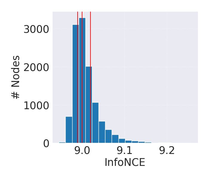
(a) GRACE

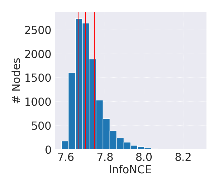
(b) GCA

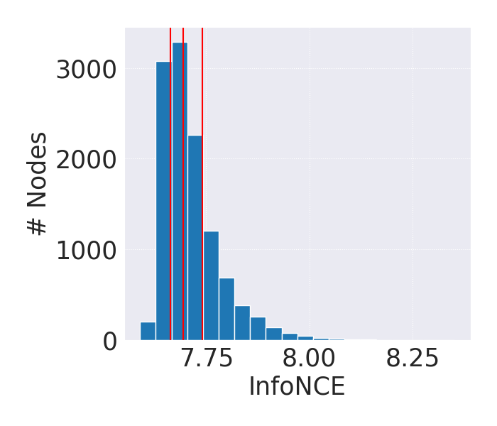
(c) ProGCL

Figure 1: The imbalance of GCL training

As mentioned in Section 1, due to the complex graph structure, we aim to investigate whether all the nodes are trained to follow the principle of GCL. Specifically, we design an experiment by plotting the distribution of InfoNCE loss values of the nodes. To illustrate the result of a GCL method, we sample 500 pairs of augmented graphs with the same augmentation strategy in the GCL method and obtain the average values of InfoNCE loss. We show the results of GRACE [35], GCA [36], and ProGCL [25] on WikiCS [14] in Figure 1 with histograms. The vertical red lines represent 1/4-quantile, median, and 3/4-quantile from left to right. The results imply that the nodes do not follow the GCL principle well enough in two aspects: 1) the InfoNCE loss of the nodes has a high variance; 2) It is shown that the untrained nodes (with higher InfoNCE loss values) are much further away from the median than the well-trained nodes (with lower InfoNCE loss values), indicating an imbalanced training in the untrained nodes. GCL methods should focus more on those untrained nodes. Therefore, it is highly desired that we should closely examine the property of different nodes so that the nodes can be trained as we expected in a provable way. Results on more datasets can be found in Appendix LABEL:sec:_more-res.

4 Methodology

4.1 Evaluating How the Nodes Follow the GCL Principle

In this section, we aim to define a metric that measures the extent of a node following the GCL principle. Since how the nodes follow the GCL principle relies on the complex graph structure generated by augmentation, the metric should be related to the set of all possible augmentations. Because InfoNCE loss can only measure the training of a node under two pre-determined augmentations, which does not meet the requirement, we propose a new metric as follows:

Definition 1 (Node Compactness).

Let $f$ denote the encoder of Graph Contrastive Learning. The compactness of node $i$ is defined as

$$\underline{\tilde{f}}_{1,i}=\min_{\begin{subarray}{c}G_{1}=(\mathbf{X},\mathbf{A}_{1})\in\mathcal{G};\\ G_{2}=(\mathbf{X},\mathbf{A}_{2})\in\mathcal{G}\end{subarray}}\{\frac{1}{N-1}\sum_{j\neq i}(\mathbf{z}_{1,i}\cdot\bar{\mathbf{z}}_{2,i}-\mathbf{z}_{1,i}\cdot\bar{\mathbf{z}}_{2,j})\ |\ \mathbf{Z}_{1}=f_{\theta}(\mathbf{X},\mathbf{A}_{1}),\mathbf{Z}_{2}=f_{\theta}(\mathbf{X},\mathbf{A}_{2})\}.$$ (2)

where $\bar{\mathbf{z}}=\mathbf{z}/\left\|\mathbf{z}\right\|_{2}$ is the normalized vector.

Definition 1 measures how worse node $i$ follows the GCL principle in all possible augmentations. If $\underline{\tilde{f}}_{i}$ is greater than zero, on average, the node embedding $\mathbf{z}_{1,i}$ is closer to the embedding of the positive sample $\mathbf{z}_{2,i}$ than the embedding of the negative sample $\mathbf{z}_{2,j}$ in the worst case of augmentation; otherwise, the embeddings of negative samples are closer. Note that normalization is used to eliminate the effect of a vector’s scale. In Definition 1, the anchor node is node $i$ in $G_{1}$, so similarly we can define $\underline{\tilde{f}}_{2,i}$ if the anchor node is node $i$ in $G_{2}$.

We can just take one of $G_{1}$ and $G_{2}$ as the variable, for example, set $G_{2}$ to be a specific sampled augmentation and $G_{1}$ to be an augmentation within the set $\mathcal{G}$. From this perspective, based on Definition 1, we can also obtain a metric, which has only one variable:

Definition 2 ($G_{2}$-Node Compactness).

Under Definition 1, if $G_{2}$ is the augmentation sampled in an epoch of GCL training, then the $G_{2}$-Node Compactness is

$$\underline{\tilde{f}}_{G_{2},i}=\min_{G_{1}=f_{\theta}(\mathbf{X},\mathbf{A}_{1})\in\mathcal{G}}\{\mathbf{z}_{1,i}\cdot\mathbf{W}^{CL}_{2,i}\ |\ \mathbf{Z}_{1}=f_{\theta}(\mathbf{X},\mathbf{A}_{1})\},$$ (3)

where $\mathbf{W}^{CL}_{2,i}=\bar{\mathbf{z}}_{2,i}-\frac{1}{N-1}\sum_{j\neq i}\bar{\mathbf{z}}_{2,j}$ is a constant vector.

Similarly, we can define $G_{1}$-node compactness $\underline{\tilde{f}}_{G_{1},i}$. Usually we have $\underline{\tilde{f}}_{G_{1},i}\geq\underline{\tilde{f}}_{2,i}$ and $\underline{\tilde{f}}_{G_{2},i}\geq\underline{\tilde{f}}_{1,i}$, i.e., $G_{1}$-node compactness and $G_{2}$-node compactness are upper bounds of node compactness.

4.2 Provable Training of GCL

To enforce the nodes to better follow the GCL principle, we optimize $G_{1}$-node compactness and $G_{2}$-node compactness in Definition 2. Designing the objective can be viewed as implicitly performing a "binary classification": the "prediction" is $\min_{G_{1}}z_{1,i}\cdot W^{CL}_{2,i}$, and the "label" is 1, which means that we expect the embedding of the anchor more likely to be classified as a positive sample in the worst case. To conclude, we propose the PrOvable Training (POT) for GCL, which provably enforces the nodes to be trained more aligned with the GCL principle. Specifically, we use binary cross-entropy as a regularization term:

$$\mathcal{L}_{\text{POT}}(G_{1},G_{2})=\frac{1}{2}(\mathcal{L}_{\text{BCE}}(\underline{\tilde{f}}_{G_{1}},\textbf{1}_{n})+\mathcal{L}_{\text{BCE}}(\underline{\tilde{f}}_{G_{2}},\textbf{1}_{n})),$$ (4)

where $\mathcal{L}_{\text{BCE}}(x,y)=-\sum_{i=1}^{N}(y_{i}\log\sigma(x_{i})+(1-y_{i})\log(1-\sigma(x_{i})))$, $\sigma$ is the sigmoid activation, $\textbf{1}_{N}=[1,1,\dots,1]\in\mathbb{R}^{N}$, and $\underline{\tilde{f}}_{G_{2}}=[\underline{\tilde{f}}_{G_{2},1},\underline{\tilde{f}}_{G_{2},2},\dots,\underline{\tilde{f}}_{G_{2},N}]$ is the vector of the lower bounds in Eq. 3. Overall, we add this term to the original InfoNCE objective and the loss function is

$$\mathcal{L}=(1-\kappa)\mathcal{L}_{\text{InfoNCE}}(Z_{1},Z_{2})+\kappa\mathcal{L}_{\text{POT}}(G_{1},G_{2}),$$ (5)

where $\kappa$ is the hyperparameter balancing the InfoNCE loss and the compactness loss. Since $G_{1}$-node compactness and $G_{2}$-node compactness are related to the network parameter $\theta$, $\mathcal{L}_{\text{POT}}$ can be naturally integrated into the loss function, which can regularize the network parameters to encode node embeddings more likely to follow the GCL principle better.

4.3 Deriving the Lower Bounds

In Section 4.2, we have proposed the formation of our loss function, but the lower bounds $\underline{\tilde{f}}_{G_{1}}$ and $\underline{\tilde{f}}_{G_{2}}$ are still to be solved. In fact, to see Eq. 3 from another perspective, $\underline{\tilde{f}}_{G_{1},1}$ (or $\underline{\tilde{f}}_{G_{2},1}$) is the lower bound of the output of the neural network concatenating a GCN encoder and a linear projection with parameter $\mathbf{W}^{CL}_{1,i}$ (or $\mathbf{W}^{CL}_{2,i}$). It is difficult to find the particular $G_{1}$ which minimizes Eq. 3, since finding that exact solution $G_{1}$ can be an NP-hard problem considering the discreteness of graph augmentations. Therefore, inspired by the bound propagation methods [5, 32, 38], we derive the output lower bounds of that concatenated network in a bound propagation manner, i.e., we can derive the lower bounds $\underline{\tilde{f}}_{G_{1}}$ and $\underline{\tilde{f}}_{G_{2}}$ by propagating the bounds of the augmented adjacency matrix $\mathbf{A}_{1}$.

However, there are still two challenges when applying bound propagation to our problem: 1) $\mathbf{A}_{1}$ in Eq. 3 is not defined as continuous values with element-wise bounds; 2) to do the propagation process, the nonlinearities in the GCN encoder $f_{\theta}$ should be relaxed.

Defining the adjacency matrix with continuous values

First, we define the set of augmented adjacency matrices as follows:

Definition 3 (Augmented adjacency matrix).

The set of augmented adjacency matrices is

$$\mathcal{A}= \{\mathbf{\tilde{A}}\in\{0,1\}^{N\times N}|\tilde{a}_{ij}\leq a_{ij}\wedge\mathbf{\tilde{A}}=\mathbf{\tilde{A}}^{T}$$

$$\wedge\|\mathbf{\tilde{A}}-\mathbf{A}\|_{0}\leq 2Q\wedge\left\|\tilde{\mathbf{A}}_{i}-\mathbf{A}_{i}\right\|_{0}\leq q_{i}\ \forall 1\leq i\leq N\},$$

where $\mathbf{\tilde{A}}$ denotes the augmented adjacency matrix, $Q$ and $q_{i}$ are the global and local budgets of edge dropped, which are determined by the specific GCL model.

The first constraint restricts the augmentation to only edge dropping, which is a common setting in existing GCL models[35, 36, 8, 25](see more discussions in Appendix B). The second constraint is the symmetric constraint of topology augmentations.

Since the message-passing matrix is used in GNN instead of the original adjacency matrix, we further relax Definition 3 and define the set of all possible message-passing matrices, which are matrices with continuous entries as expected, inspired by [38]:

Definition 4 (Augmented message-passing matrix).

The set of augmented message-passing matrices is

$$\hat{\mathcal{A}} =\{\hat{\mathbf{A}}\in[0,1]^{N\times N}\mid\hat{\mathbf{A}}=\hat{\mathbf{A}}^{T}\wedge\forall i,j:L_{ij}\leq\hat{a}_{ij}\leq U_{ij}\},$$

$$L_{ij} =\left\{\begin{array}[]{ll}\tilde{a}_{ij}&,i=j\\ 0&,i\neq j\end{array},\right.U_{ij}=\left\{\begin{array}[]{cc}((d_{i}-q_{i})(d_{j}-q_{j}))^{-\frac{1}{2}}&,i=j\\ \min\{a_{ij},((d_{i}-q_{i})(d_{j}-q_{j}))^{-\frac{1}{2}}\}&,i\neq j\end{array},\right.$$

where $\mathbf{\hat{A}}$ denotes the augmented message-passing matrix.

Under Definition 4, the augmented message-passing matrices are non-discrete matrices with element-wise bounds $L_{ij}$ and $U_{ij}$. $L_{ij}$ is $\tilde{a}_{ij}$ when $i=j$, since there is no edge added and the self-loop can not be dropped; $L_{ij}$ is $0$ when $i\neq j$, which implies the potential dropping of each edge. $U_{ij}$ is set to $((d_{i}-q_{i})(d_{j}-q_{j}))^{-\frac{1}{2}}$ when $i=j$ because $\hat{a}_{ii}$ is the largest when its adjacent edges are dropped as much as possible, and $U_{ij}=\min\{a_{ij},((d_{i}-q_{i})(d_{j}-q_{j}))^{-\frac{1}{2}}\}$ when $i\neq j$ since there is only edge dropping, $U_{ij}$ cannot exceed $a_{ij}$.

Relaxing the nonlinearities in the GCN encoder

The GCN encoder in our problem has non-linear activation functions as the nonlinearities in the network, which is not suitable for bound propagation. Therefore, we relax the activations with linear bounds [32]:

Definition 5 (Linear bounds of non-linear activation function).

For node $i$ and the $m$-th neuron in the $k$-th layer, the input of the neuron is $p^{(k)}_{i,m}$, and $\sigma$ is the activation function of the neuron. With the lower bound and upper bound of the input denoted as $p^{(k)}_{L,i,m}$ and $p^{(k)}_{U,i,m}$, the output of the neuron is bounded by linear functions with parameters $\alpha^{(k)}_{L,i,m},\alpha^{(k)}_{U,i,m},\beta^{(k)}_{L,i,m},\beta^{(k)}_{U,i,m}\in\mathbb{R}$, i.e.

$$\alpha^{(k)}_{L,i,m}(p^{(k)}_{i,m}+\beta^{(k)}_{L,i,m})\leq\sigma(p^{(k)}_{i,m})\leq\alpha^{(k)}_{U,i,m}(p^{(k)}_{i,m}+\beta^{(k)}_{U,i,m}).$$

The values of $\alpha^{(k)}_{L,i,m},\alpha^{(k)}_{U,i,m},\beta^{(k)}_{L,i,m},\beta^{(k)}_{U,i,m}$ depend on the activation $\sigma$ and the pre-activation bounds $p^{(k)}_{L,i,m}$ and $p^{(k)}_{U,i,m}$.

To further obtain $\alpha$ and $\beta$, we compute the pre-activation bounds $\mathbf{P}^{(k)}_{L}$ and $\mathbf{P}^{(k)}_{U}$ as follows, which is the matrix with elements $p^{(k)}_{L,i,m}$ and $p^{(k)}_{U,i,m}$:

Theorem 1 (Pre-activation bounds of each layer [16]).

If $f=\sigma(\mathbf{\hat{A}}\sigma(\mathbf{\hat{A}}\mathbf{X}\mathbf{\mathbf{W^{(1)}}}+\mathbf{b}^{(1)})\mathbf{\mathbf{W^{(2)}}}+\mathbf{b}^{(2)})$ is the two-layer GCN encoder, given the element-wise bounds of $\mathbf{\hat{A}}$ in Definition 4, $\mathbf{H}^{(k)}$ is the input embedding of $t$-th layer, then the pre-activation bounds of $t$-th layer are

$$\mathbf{P}^{(k)}_{L} =\mathbf{L}[\mathbf{H}^{(k)}\mathbf{W}^{(k)}]_{+}+\mathbf{U}[\mathbf{H}^{(k)}\mathbf{W}^{(k)}]_{-}+\mathbf{b}^{(k)},$$

$$\mathbf{P}^{(k)}_{U} =\mathbf{U}[\mathbf{H}^{(k)}\mathbf{W}^{(k)}]_{+}+\mathbf{L}[\mathbf{H}^{(k)}\mathbf{W}^{(k)}]_{-}+\mathbf{b}^{(k)},$$

where $[\mathbf{X}]_{+}=\max(\mathbf{X},0)$ and $[\mathbf{X}]_{-}=\min(\mathbf{X},0)$.

The detailed proof is provided in Appendix A.1. Therefore, $p^{(k)}_{L,i,m}$ and $p^{(k)}_{U,i,m}$ are known with Theorem 1 given, then the values of $\alpha$ and $\beta$ can be obtained by referring to Table 1. In the table, we denote $p^{(k)}_{U,i,m}$ as $u$ and $p^{(k)}_{L,i,m}$ as $l$ for short. $\gamma$ is the slope parameter of ReLU-like activation functions that are usually used in GCL, such as ReLU, PReLU, and RReLU. For example, $\gamma$ is zero for ReLU.

Table 1: Values of $\alpha$ and $\beta$

	$l\geq 0$	$u\leq 0$	else
$\alpha^{(k)}_{L,i,m}$	$1$	$\gamma$	$\frac{u-\gamma l}{u-l}$
$\alpha^{(k)}_{U,i,m}$	$1$	$\gamma$	$\frac{u-\gamma l}{u-l}$
$\beta^{(k)}_{L,i,m}$	$0$	$0$	$0$
$\beta^{(k)}_{U,i,m}$	$0$	$0$	$\frac{(\gamma-1)ul}{u-\gamma l}$

To this end, all the parameters to derive the lower bounds $\underline{\tilde{f}}_{G_{1}}$ and $\underline{\tilde{f}}_{G_{2}}$ are known: the bounds of the variable $\mathbf{\hat{A}}$ in our problem, which are $\mathbf{L}$ and $\mathbf{U}$ defined in Definition 4; the parameters of the linear bounds for non-linear activations, which are $\alpha$ and $\beta$ defined in Definition 5 and obtained by Theorem 1 and Table 1. To conclude, the whole process is summarized in the following theorem, where we apply bound propagation to our problem with those parameters:

Theorem 2 (The lower bound of neural network output).

If the encoder is defined as 1, $\mathbf{\hat{A}}$ is the augmented message-passing matrix and $\sigma$ is the non-linear activation function, for $G_{1}=(\mathbf{X},\mathbf{A}_{1})\in\mathcal{G}$, $\mathbf{\hat{A}}=\mathbf{D}^{-1/2}(\mathbf{A}_{1}+\mathbf{I})\mathbf{D}^{-1/2}\in\hat{\mathcal{A}}$, then

$$\underline{\tilde{f}}_{G_{2},i} =\sum_{j_{1}\in\mathcal{N}(i)}\hat{a}_{j_{1}i}[\sum_{j_{2}\in\mathcal{N}(j_{1})}\hat{a}_{j_{2}j_{1}}x_{j_{2}}\mathbf{\tilde{W}}^{(1)}_{i}+\mathbf{\tilde{b}}^{(1)}]+\mathbf{\tilde{b}}^{(2)}$$ (6)

where $$\mathbf{W}^{CL}_{2,i}=\bar{\mathbf{z}}_{2,i}-\frac{1}{N-1}\sum_{j\neq i}\bar{\mathbf{z}}_{2,j},\ \mathcal{N}(i)=\{j\ |\ a_{ij}>0\text{ or }j=i\},$$ (7)

$$\lambda_{i,m}^{(2)}=\left\{\begin{array}[]{ll}\alpha_{L,i,m}^{(2)}&\text{if }W^{CL}_{2,i,m}\geq 0\\ \alpha_{U,i,m}^{(2)}&\text{if }W^{CL}_{2,i,m}<0\\ \end{array}\right.,\ \Delta_{i,m}^{(2)}=\left\{\begin{array}[]{ll}\beta_{L,i,m}^{(2)}&\text{if }W^{CL}_{2,i,m}\geq 0\\ \beta_{U,i,m}^{(2)}&\text{if }W^{CL}_{2,i,m}<0\\ \end{array}\right.$$ (12)

$$\Lambda^{(2)}_{i}=W^{CL}_{2,i}\odot\lambda^{(2)}_{i},\ \mathbf{\tilde{W}^{(2)}}_{i}=\sum_{m=1}^{d_{2}}\Lambda^{(2)}_{i,m}W_{:,m}^{(2)},\ \tilde{b}^{(2)}_{i}=\sum_{m=1}^{d_{2}}\Lambda^{(2)}_{i,m}(b_{m}^{(2)}+\Delta_{i,m}^{(2)}),$$ (13)

$$\lambda_{i,m}^{(1)}=\left\{\begin{array}[]{ll}\alpha_{L,i,m}^{(1)}&\text{if }\tilde{W}^{(2)}_{i,m}\geq 0\\ \alpha_{U,i,m}^{(1)}&\text{if }\tilde{W}^{(2)}_{i,m}<0\\ \end{array}\right.,\ \Delta_{i,l}^{(1)}=\left\{\begin{array}[]{ll}\beta_{L,i,l}^{(1)}&\text{if }\tilde{W}^{(2)}_{i,l}\geq 0\\ \beta_{U,i,l}^{(1)}&\text{if }\tilde{W}^{(2)}_{i,l}<0\\ \end{array}\right.$$ (18)

$$\mathbf{\Lambda}^{(1)}=\mathbf{\tilde{W}}^{(2)}_{i}\odot\mathbf{\lambda^{(1)}},\ \mathbf{\tilde{W}}^{(1)}_{i}=\sum_{l=1}^{d_{1}}\Lambda^{(1)}_{i,l}\mathbf{W}_{:,l}^{(1)},\ \mathbf{\tilde{b}}^{(1)}_{i}=\sum_{l=1}^{d_{2}}\Lambda^{(1)}_{i,l}(b_{m}^{(1)}+\Delta_{i,l}^{(1)}).$$ (19)

$\mathbf{\lambda}^{(2)}_{i},\ \mathbf{\Delta}^{(2)}_{i},\ \mathbf{\Lambda}^{(2)}_{i}\in\mathbb{R}^{d_{2}}$; $\mathbf{\lambda}^{(1)}_{i},\ \mathbf{\Delta}^{(1)}_{i},\ \mathbf{\Lambda}^{(1)}_{i}\in\mathbb{R}^{d_{1}}$; $\mathbf{\tilde{W}}^{(2)}_{i},\ \mathbf{\tilde{W}}^{(1)}_{i}\in\mathbb{R}^{F\times 1}$; $\mathbf{\tilde{b}}^{(2)},\ \mathbf{\tilde{b}}^{(1)}\in\mathbb{R}$; $d_{1}$ and $d_{2}$ are the dimension of the embedding of layer 1 and layer 2 respectively.

We provide detailed proof in Appendix A.2. Theorem 2 demonstrates the process of deriving the node compactness $\underline{\tilde{f}}_{G_{2},i}$ in a bound propagation manner. Before Theorem 2, we obtain all the parameters needed, and we apply the bound propagation method [32] to our problem, which is the concatenated network of the GCN encoder $f_{\theta}$ and a linear transformation $W^{CL}_{2,i}$.As the form of Eq. 6, the node compactness $\underline{\tilde{f}}_{G_{2},i}$ can be also seen as the output of a new "GCN" encoder with network parameters $\mathbf{\tilde{W}^{(1)}}_{i}$, $\mathbf{\tilde{b}^{(1)}}$, $\tilde{b}^{(2)}$, which is an encoder constructed from the GCN encoder in GCL.Additionally, we present the whole process of our POT method inAlgorithm 1.

1

Input : Graph $G=(\mathbf{X},\mathbf{A})$, the set of all possible augmentations $\mathcal{G}$

Output : Node embeddings $\mathbf{Z}_{1}$ and $\mathbf{Z}_{2}$

2 Initialize GNN encoder paramenters $\{\mathbf{W}^{(1)},\mathbf{b}^{(1)},\mathbf{W}^{(2)},\mathbf{b}^{(2)}\}$;

3 while not converge do

4       Generate graph augmentations $G_{1}=(\mathbf{X},\mathbf{\tilde{A}}_{1})$ and $G_{2}=(\mathbf{X},\mathbf{\tilde{A}}_{2})$;

5       Do forward pass, obtain $\mathbf{Z}_{1}=f_{\theta}(\mathbf{X},\mathbf{\tilde{A}}_{1})$ and $\mathbf{Z}_{2}=f_{\theta}(\mathbf{X},\mathbf{\tilde{A}}_{2})$, calculate $\mathcal{L}_{\text{InfoNCE}}$;

6       Obtain the pre-activation bounds $\{\mathbf{P}^{(k)}_{L},\mathbf{P}^{(k)}_{U}\},\ k=1,2$ as in Theorem 1;

7       Set $\{\alpha^{(k)}_{L},\alpha^{(k)}_{U},\beta^{(k)}_{L},\beta^{(k)}_{U}\},\ k=1,2$ according to Table 1;

8       Derive $\underline{\tilde{f}}_{G_{1},i}$, $\underline{\tilde{f}}_{G_{2},i}$ as in Theorem 2 for $i=1$ to $N$ and calculate $\mathcal{L}_{\text{POT}}$ as in Equation 4;

9       Do backward propagation with $\mathcal{L}=(1-\kappa)\mathcal{L}_{\text{InfoNCE}}(\mathbf{Z}_{1},\mathbf{Z}_{2})+\kappa\mathcal{L}_{\text{POT}}(G_{1},G_{2})$;

10      

11 end while

12return $\mathbf{Z}_{1}$, $\mathbf{Z}_{2}$ for downstream tasks;

Algorithm 1 Provable Training for GCL

Time Complexity

The computation of the weight matrices in Theorem 2 dominates the time complexity of POT. Thus, the time complexity of our algorithm is $O(Nd_{k-1}d_{k}+Ed_{k})$ for the $k$-th layer, which is the same as the message-passing [4, 10] in the GNN encoders.

5 Experiments

5.1 Experimental Setup

We choose four GCL baseline models for evaluation: GRACE [35], GCA [36], ProGCL [25], and COSTA [34]. Since POT is a plugin for InfoNCE loss, we integrate POT with the baselines and construct four models: GRACE-POT, GCA-POT, ProGCL-POT, and COSTA-POT. Additionally, we report the results of two supervised baselines: GCN and GAT [20]. For the benchmarks, we choose 8 common datasets: Cora, CiteSeer, PubMed [28], Flickr, BlogCatalog [13], Computers, Photo [18], and WikiCS [14]. Details of the datasets and baselines are presented in Appendix C.2. For datasets with a public split available [28], including Cora, CiteSeer, and PubMed, we follow the public split; For other datasets with no public split, we generate random splits, where each of the training set and validation set contains 10% nodes of the graph and the rest 80% nodes of the graph is used for testing.

5.2 Node Classification

Table 2: Performance ($\%\pm\sigma$) on Node Classification

GRACE GCA ProGCL COSTA Datasets Metrics GCN GAT w/o POT w/ POT w/o POT w/ POT w/o POT w/ POT w/o POT w/ POT Cora Mi-F1 $81.9\pm 1.1$ $82.8\pm 0.5$ $78.2\pm 0.6$ $\mathbf{79.2\pm 1.2}$ $78.6\pm 0.2$ $\mathbf{79.6\pm 1.4}$ $77.9\pm 1.4$ $\mathbf{79.9\pm 1.0}$ $79.9\pm 0.7$ $\mathbf{80.5\pm 0.9}$ Ma-F1 $80.6\pm 1.1$ $81.8\pm 0.3$ $76.8\pm 0.6$ $\mathbf{77.8\pm 1.4}$ $77.7\pm 0.1$ $\mathbf{79.1\pm 1.4}$ $77.3\pm 1.7$ $\mathbf{78.8\pm 0.9}$ $79.5\pm 0.7$ $\mathbf{80.1\pm 0.8}$ CiteSeer Mi-F1 $71.6\pm 0.6$ $72.1\pm 1.0$ $66.8\pm 1.0$ $\mathbf{68.7\pm 0.6}$ $65.0\pm 0.7$ $\mathbf{69.0\pm 0.8}$ $65.9\pm 0.9$ $\mathbf{67.7\pm 0.9}$ $66.8\pm 0.8$ $\mathbf{67.9\pm 0.7}$ Ma-F1 $68.2\pm 0.5$ $67.1\pm 1.3$ $63.2\pm 1.3$ $\mathbf{64.0\pm 0.9}$ $60.8\pm 0.8$ $\mathbf{65.5\pm 0.7}$ $62.5\pm 0.9$ $\mathbf{63.6\pm 0.5}$ $63.4\pm 1.4$ $\mathbf{64.0\pm 1.2}$ PubMed Mi-F1 $79.3\pm 0.1$ $78.3\pm 0.7$ $81.6\pm 0.5$ ${82.0\pm 1.3}$ $80.5\pm 2.3$ $\mathbf{82.8\pm 2.0}$ $81.5\pm 1.1$ ${81.9\pm 0.4}$ $80.0\pm 1.5$ $\mathbf{80.6\pm 1.3}$ Ma-F1 $79.0\pm 0.1$ $77.6\pm 0.8$ $81.7\pm 0.5$ $\mathbf{82.4\pm 1.2}$ $80.5\pm 2.1$ $\mathbf{82.9\pm 2.0}$ $81.3\pm 1.0$ $\mathbf{82.2\pm 0.4}$ $79.3\pm 1.4$ $\mathbf{80.3\pm 1.5}$ Flickr Mi-F1 $48.8\pm 1.9$ $37.3\pm 0.5$ $46.5\pm 1.8$ $\mathbf{48.4\pm 1.3}$ $47.4\pm 0.8$ $\mathbf{50.3\pm 0.3}$ $46.4\pm 1.4$ $\mathbf{49.7\pm 0.5}$ $52.6\pm 1.2$ $\mathbf{53.8\pm 1.2}$ Ma-F1 $45.8\pm 2.4$ $35.2\pm 0.7$ $45.1\pm 1.4$ $\mathbf{47.0\pm 1.6}$ $46.2\pm 0.8$ $\mathbf{49.3\pm 0.4}$ $45.4\pm 1.1$ $\mathbf{48.9\pm 0.3}$ $51.2\pm 0.9$ $\mathbf{52.6\pm 1.3}$ BlogCatalog Mi-F1 $72.4\pm 2.5$ $68.0\pm 2.1$ $70.5\pm 1.3$ $\mathbf{72.4\pm 1.4}$ $76.2\pm 0.6$ ${76.5\pm 0.5}$ $74.1\pm 0.6$ $\mathbf{76.0\pm 0.7}$ $73.3\pm 3.4$ $\mathbf{75.1\pm 1.5}$ Ma-F1 $71.9\pm 2.4$ $67.6\pm 1.8$ $70.2\pm 1.3$ $\mathbf{71.8\pm 1.4}$ $75.8\pm 0.7$ ${76.1\pm 0.5}$ $73.7\pm 0.6$ $\mathbf{75.7\pm 0.9}$ $73.0\pm 3.6$ $\mathbf{74.9\pm 1.6}$ Computers Mi-F1 $87.6\pm 0.6$ $88.7\pm 1.3$ $85.9\pm 0.4$ $\mathbf{86.9\pm 0.7}$ $88.7\pm 0.6$ $\mathbf{89.1\pm 0.3}$ $88.6\pm 0.7$ $\mathbf{89.0\pm 0.5}$ $82.5\pm 0.4$ ${82.8\pm 0.7}$ Ma-F1 $83.1\pm 2.3$ $79.3\pm 1.4$ $83.9\pm 0.8$ $\mathbf{84.5\pm 1.4}$ $87.1\pm 0.7$ $\mathbf{87.6\pm 0.5}$ $86.9\pm 1.1$ $\mathbf{87.4\pm 0.9}$ $78.8\pm 1.7$ ${79.0\pm 1.0}$ Photo Mi-F1 $91.7\pm 0.7$ $92.0\pm 0.5$ $91.2\pm 0.4$ $\mathbf{91.8\pm 0.3}$ $91.5\pm 0.4$ $\mathbf{92.0\pm 0.3}$ $92.1\pm 0.3$ $\mathbf{92.4\pm 0.3}$ $91.5\pm 0.6$ $\mathbf{92.2\pm 1.0}$ Ma-F1 $88.8\pm 2.0$ $88.9\pm 2.2$ $89.2\pm 0.7$ $\mathbf{90.0\pm 0.6}$ $89.5\pm 0.5$ $\mathbf{90.0\pm 0.6}$ $90.6\pm 0.6$ $\mathbf{90.9\pm 0.6}$ $89.3\pm 1.3$ $\mathbf{90.1\pm 1.4}$ WikiCS Mi-F1 $81.2\pm 1.2$ $81.2\pm 0.8$ $80.3\pm 0.3$ $\mathbf{80.6\pm 0.3}$ $78.7\pm 0.3$ $\mathbf{80.7\pm 0.3}$ $78.8\pm 0.4$ $\mathbf{80.0\pm 0.5}$ $76.2\pm 1.6$ $\mathbf{79.1\pm 0.9}$ Ma-F1 $78.7\pm 1.9$ $78.5\pm 1.8$ $77.6\pm 0.3$ $\mathbf{78.0\pm 0.3}$ $75.4\pm 0.1$ $\mathbf{78.0\pm 0.3}$ $75.6\pm 0.3$ $\mathbf{77.2\pm 0.8}$ $72.2\pm 1.6$ $\mathbf{75.8\pm 0.8}$

We test the performance of POT on node classification. For the evaluation process, we follow the setting in baselines [35, 36, 25, 34] as follows: the encoder is trained in a contrastive learning manner without supervision, then we obtain the node embedding and use the fixed embeddings to train and evaluate a logistic regression classifier on the downstream node classification task. We choose two measures: Micro-F1 score and Macro-F1 score. The results with error bars are reported in Table 5.2. Bolded results mean that POT outperforms the baseline, with a t-test level of 0.1. As it shows, our POT method improves the performance of all the base models consistently on all datasets, which verifies the effectiveness of our model. Moreover, POT gains significant improvements over baseline models on BlogCatalog and Flickr. These two datasets are the graphs with the highest average node degree, therefore there are more possible graph augmentations in these datasets (the higher node degrees are, the more edges are dropped  [35, 36]). This result illustrates our motivation that POT improves existing GCL methods when faced with complex graph augmentations.

5.3 Analyzing the Node Compactness

To illustrate how POT improves the training of GCL, we conduct experiments to show some interesting properties of POT by visualizing the node compactness in Definition 2.

POT Improves Node Compactness. We illustrate that our POT does improve the node compactness, which is the goal of InfoNCE. The result on Cora is shown in Figure 2. The x-axis is the epoch number and the y-axis is the average compactness of all nodes. We can see that the node compactness of the model with POT is almost always higher than the model without POT, indicating that POT increases node compactness in the training of GCL, i.e. how the nodes follow the GCL principle is improved in the worst-case. Therefore, our POT promotes nodes to follow the GCL principle better. More results on BlogCatalog are shown in Appendix LABEL:sec:_more-res.

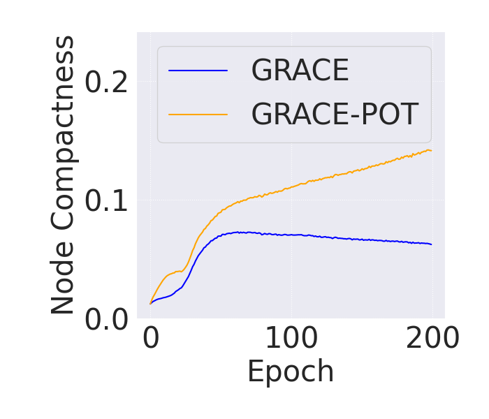
(a) GRACE

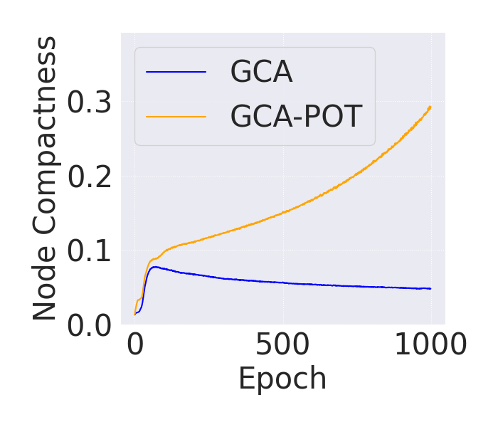
(b) GCA

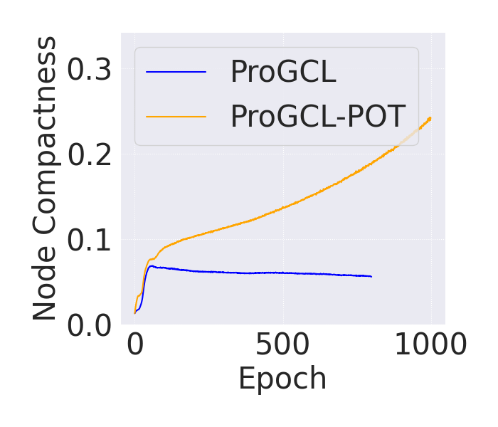
(c) ProGCL

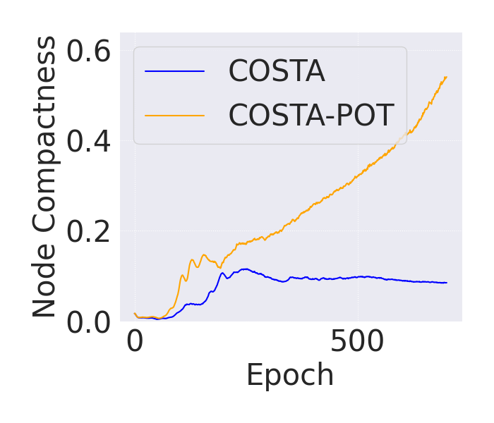
(d) COSTA

Figure 2: Node compactness in the training process

Node Compactness Reflects Different Properties of Different Augmentation Strategies. There are two types of augmentation strategies: GRACE adapts a constant dropping rate, then the dropping rate of edges in a node’s neighborhood ("neighbor dropping rate" for short) does not change among different nodes; GCA, however, adapts a larger dropping rate on edges that are adjacent to higher-degree nodes, then the neighbor dropping rate is larger for higher-degree nodes. According to Definition 2, since node compactness is how a node follows the GCL principle in the worst case, a higher degree results in larger node compactness, while a higher neighbor dropping rate results in lower node compactness because worse augmentations can be taken. To see whether node compactness can reflect those properties of different augmentation as expected, we plot the average node compactness of the nodes with the same degree as scatters in Figure 3 on BlogCatalog and Flickr. For GRACE, node degree and compactness are positively correlated, since the neighbor dropping rate does not change with a higher degree; For GCA, node compactness reflects a trade-off between neighbor dropping rate and degree: the former dominates in the low-degree stage then the latter dominates later, resulting the curve to drop then slightly rise. To conclude, node compactness can reflect the properties of different augmentation strategies.

(a) GRACE, BlogCatalog

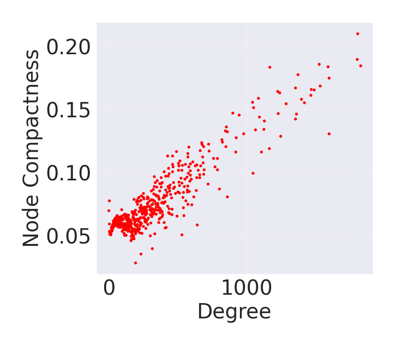
(b) GRACE, Flickr

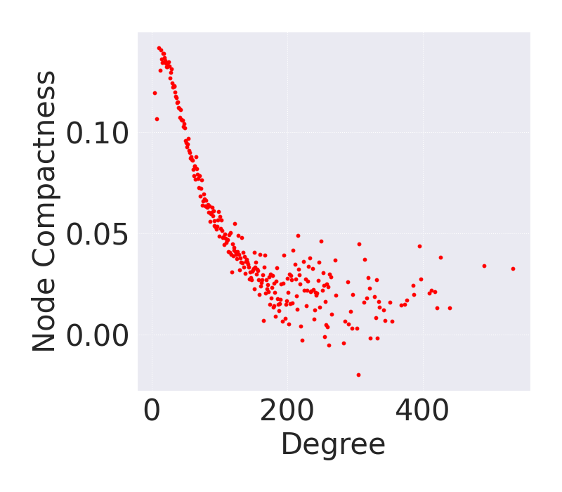
(c) GCA, BlogCatalog

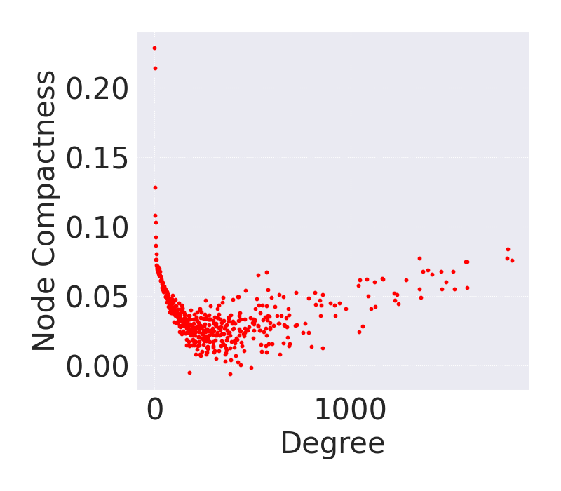
(d) GCA, Flickr

Figure 3: Degree and node compactness score

5.4 Hyperparameter Analysis

In this subsection, we investigate the sensitivity of the hyperparameter in POT, $\kappa$ in Eq. 5. In our experiments, we tune $\kappa$ ranging from {$0.5,0.4,0.3,0.2,0.1,0.05$}. The hyperparameter $\kappa$ balances between InfoNCE loss and POT, i.e. the importance of POT is strengthened when $\kappa>0.5$ while the InfoNCE is more important when $\kappa<0.5$. We report the Micro-F1 score on node classification of BlogCatalog in Figure 4. Although the performance is sensitive to the choice of $\kappa$, the models with POT can still outperform the corresponding base models in many cases, especially on BlogCatalog where POT outperforms the base models whichever $\kappa$ is selected. The result on Cora is in Appendix LABEL:sec:_more-res.

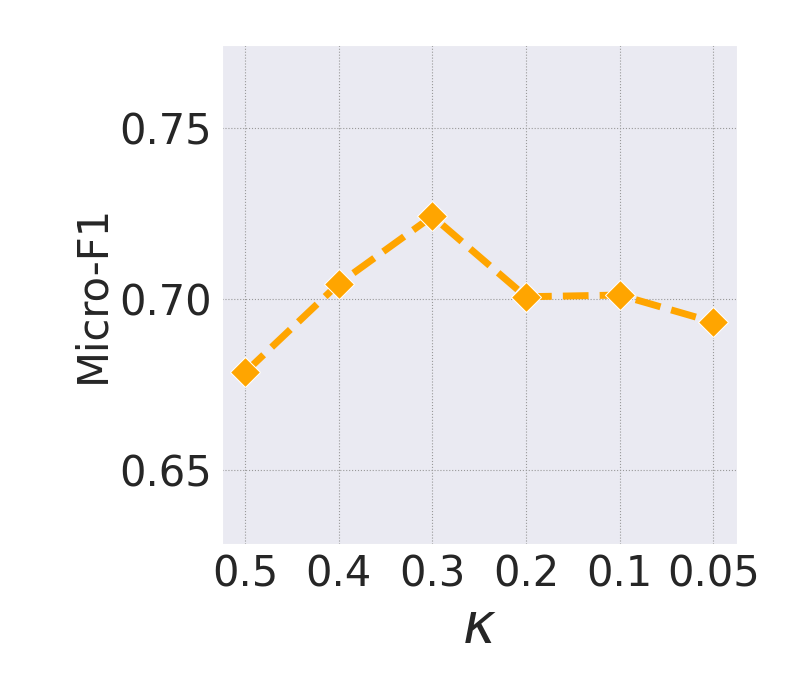
(a) GRACE-POT

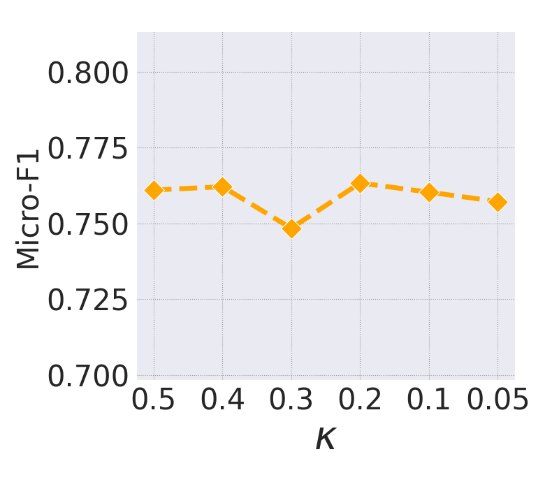
(b) GCA-POT

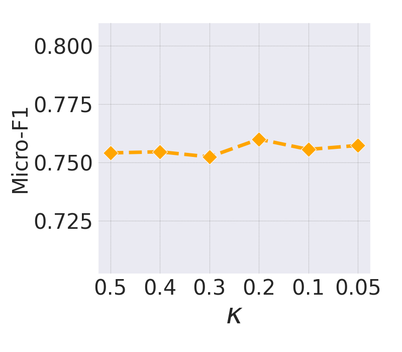
(c) ProGCL-POT

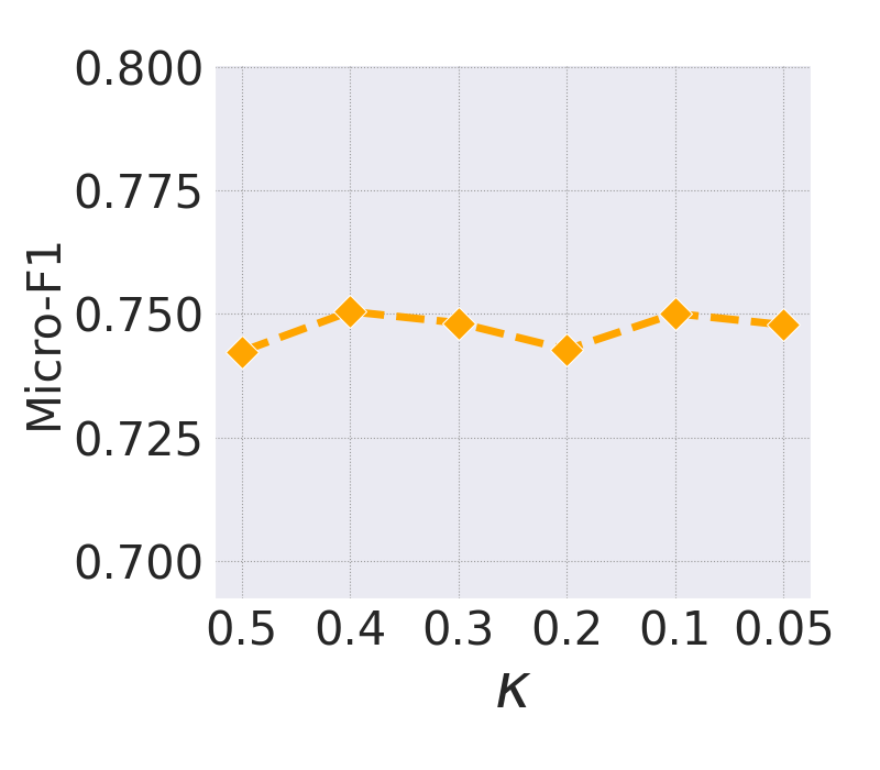
(d) COSTA-POT

Figure 4: Hyperparamenter analysis on $\kappa$

6 Related Work

Graph Contrastive Learning. Graph Contrastive Learning (GCL) methods are proposed to learn the node embeddings without the supervision of labels. GRACE [35] firstly proposes GCL with random edge dropping and feature masking as data augmentations and takes InfoNCE as the objective. Based on GRACE, GCA [36] improves the data augmentation with adaptive masking and dropping rate related to node centrality. COSTA [34] proposes feature augmentation in embedding space to reduce sampling bias. ProGCL [25] reweights the negatives and empowers GCL with hard negative mining. There are also node-to-graph GCL methods, like DGI [21] and MVGRL [8]. Inspired by BYOL [6], there are also several GCL methods that do not need negative samples [19] or use BCE objectives [31].

Bound Propagation. Bound Propagation methods derive the output bounds directly from input bounds. Interval Bound Propagation [5] defines the input adversarial polytope as a $l_{\infty}$-norm ball, and it deforms as being propagated through affine layers and monotonic activations. [16] proposes a relaxation on nonlinearity via Semidefinite Programming but is restricted to one hidden layer. [24] relaxes ReLU via convex outer adversarial polytope. [32] can be applied to general activations bounded by linear functions. For GNN, [37] and [38] study the bound propagation on GNN with feature and topology perturbations respectively. One step further, [17] proposes a Mixed Integer Linear Programming based method to relax GNN certification with a shared perturbation as input. However, almost all the previous works require solving an optimization problem with some specific solver, which is time-consuming and impossible to be integrated into a training process as we expected.

7 Conclusion

In this paper, we investigate whether the nodes follow the GCL principle well enough in GCL training, and the answer is no. Therefore, to address this issue, we design the metric "node compactness" to measure the training of each node, and we propose POT as a regularizer to optimize node compactness, which can be plugged into the existing InfoNCE objective of GCL. Additionally, we provide a bound propagation-inspired method to derive POT theoretically. Extensive experiments and insightful visualizations verify the effectiveness of POT on various GCL methods.

Limitations and broader impacts. One limitation of our work is the restriction on the settings of GCL. To extend our work to more types of GCL settings and graph-level GCL, one can define the set of augmentations and network structure properly, then follow the proof in Appendix A.2 to derive the node compactness in a new setting. The detailed discussion can be found in Appendix B. We leave them for future work. Moreover, there are no negative social impacts foreseen.

Appendix A Proofs and Derivations

A.1 Proof of Theorem 1

Proof.

We mainly make use of a conclusion in [16] and express it as the lemma below:

Lemma 1 (Bound propagation of affine layers [16]).

In an affine layer $\mathbf{x}^{k}=\mathbf{W}^{k-1}\mathbf{x}^{k-1}+\mathbf{b}^{k-1}$, the lower bound $\mathbf{l}^{k}$ and upper bound $\mathbf{u}^{k}$ of $k$-th layer after affine transformation can be obtained by

$$\mathbf{l}^{k}=[\mathbf{W}^{k-1}]_{+}\mathbf{l}^{k-1}+[\mathbf{W}^{k-1}]_{-}\mathbf{u}^{k-1}+\mathbf{b}^{k-1},\ \mathbf{u}^{k}=[\mathbf{W}^{k-1}]_{+}\mathbf{u}^{k-1}+[\mathbf{W}^{k-1}]_{-}\mathbf{l}^{k-1}+\mathbf{b}^{k-1},$$

where $[\mathbf{W}^{k}]_{+}=\max(\mathbf{W}^{k},0)$ and $[\mathbf{W}^{k}]_{-}=\min(\mathbf{W}^{k},0)$, $\mathbf{W}^{k}$ is the weights of affine transformation in the $k$-th layer.

In our problem, since $\hat{\mathbf{A}}$ is variable, we take $\mathbf{H}^{(k)}\mathbf{W}^{(k)}$ as the weights of the affine transformation and replace $\mathbf{l}^{k}$ and $\mathbf{u}^{k}$ with the bounds $\mathbf{L}$ and $\mathbf{U}$. To this end, Theorem 1 is proved. ∎

A.2 Proof of Theorem 2

Proof.

Since $\mathbf{H}^{(k)}$ is the output embedding of the $k$-th layer, which implies that $\mathbf{H}^{(k-1)}$ is the input embedding of $k$-th layer. $\mathbf{P}^{(k)}$ is the pre-activation embedding in Theorem 1, $f_{\theta}(\mathbf{X},A_{1})=\sigma(\mathbf{P}^{(2)}),\mathbf{P}^{(2)}=\hat{\mathbf{A}}\sigma(\mathbf{P}^{(1)})\mathbf{W}^{(2)}+\mathbf{b}^{(2)},\mathbf{P}^{(1)}=\hat{\mathbf{A}}\mathbf{X}\mathbf{W}^{(1)}+\mathbf{b}^{(1)}$. With the parameters $\alpha$, $\beta$, $\mathbf{L}$, $\mathbf{U}$ obtained, as well as the parameters of the GCN encoder {$\mathbf{W}^{(1)}$, $\mathbf{b}^{(1)}$, $\mathbf{W}^{(2)}$, $\mathbf{b}^{(2)}$} given, we can derive the lower bound $\underline{\tilde{f}}_{G_{2},i}$ in a bound propagation [32] manner, by taking $\hat{\mathbf{A}}$ as a variable with element-wise upper and lower bound in Definition 4:

$$\underline{\tilde{f}}_{G_{2},i} =\min_{\hat{\mathbf{A}}}\{\sigma(\mathbf{P}^{(2)}_{i})\cdot\mathbf{W}^{CL}_{2,i}\}$$ (20)

$$=\min_{\hat{\mathbf{A}}}\{\ \sum_{m=1}^{d_{2}}\sigma(\mathbf{P}^{(2)}_{i,m})W^{CL}_{2,i,m}\}$$ (21)

$$=\sum_{W^{CL}_{2,i,m}\geq 0}(\alpha^{(2)}_{L,i,m}(p^{(2)}_{i,m}+\beta^{(2)}_{L,i,m}))\cdot W^{CL}_{2,i,m}+\sum_{W^{CL}_{2,i,m}<0}(\alpha^{(2)}_{U,i,m}(p^{(2)}_{i,m}+\beta^{(2)}_{U,i,m}))\cdot W^{CL}_{2,i,m}$$ (22)

$$=\sum_{m=1}^{d_{2}}W^{CL}_{2,i,m}\lambda^{(2)}_{i,m}(p^{(2)}_{i,m}+\Delta^{(2)}_{i,m})$$ (23)

$$=\sum_{m=1}^{d_{2}}\Lambda^{(2)}_{i,m}(p^{(2)}_{i,m}+\Delta^{(2)}_{i,m})$$ (24)

$$=\sum_{m=1}^{d_{2}}\Lambda^{(2)}_{i,m}(\sum_{j_{1}\in\mathcal{N}(i)}\hat{a}_{j_{1}i}\sigma(\mathbf{P}^{(1)}_{i})\mathbf{W}^{(2)}_{:,m}+b^{(2)}_{m}+\Delta^{(2)}_{i,m})$$ (25)

$$=\sum_{j_{1}\in\mathcal{N}(i)}\hat{a}_{j_{1}i}\sigma(\mathbf{P}^{(1)}_{i})\mathbf{\tilde{W}}^{(2)}_{i}+\tilde{b}^{(2)}_{i}$$ (26)

$$=\sum_{j_{1}\in\mathcal{N}(i)}\hat{a}_{j_{1}i}\sum_{l=1}^{d_{1}}\mathbf{\tilde{W}}^{(2)}_{i,l}\lambda^{(1)}_{j_{1},l}(p^{(1)}_{j_{1},l}+\Delta^{(1)}_{j_{1},l})+\tilde{b}^{(2)}_{i}$$ (27)

$$=\sum_{j_{1}\in\mathcal{N}(i)}\hat{a}_{j_{1}i}\sum_{l=1}^{d_{1}}\Lambda^{(1)}_{i,l}(p^{(1)}_{j_{1},l}+\Delta^{(1)}_{j_{1},l})+\tilde{b}^{(2)}_{i}$$ (28)

$$=\sum_{j_{1}\in\mathcal{N}(i)}\hat{a}_{j_{1}i}(\sum_{j_{2}\in\mathcal{N}(j_{1})}\hat{a}_{j_{2}j_{1}}x_{j_{2}}\tilde{W}^{(1)}_{i}+\tilde{b}^{(1)})+\tilde{b}^{(2)}_{i}.$$ (29)

(21) is the equivalent form of (20), and (22) is because: since $\alpha^{(k)}_{L,i,m}(p^{(k)}_{i,m}+\beta^{(k)}_{L,i,m})\leq\sigma(p^{(k)}_{i,m})\leq\alpha^{(k)}_{U,i,m}(p^{(k)}_{i,m}+\beta^{(k)}_{U,i,m})$, then if $W^{CL}_{2,i,m}$ is multiplied to the inequality, we have

$$\alpha^{(k)}_{L,i,m}(p^{(k)}_{i,m}+\beta^{(k)}_{L,i,m})W^{CL}_{2,i,m}\leq\sigma(p^{(k)}_{i,m})W^{CL}_{2,i,m}\leq\alpha^{(k)}_{U,i,m}(p^{(k)}_{i,m}+\beta^{(k)}_{U,i,m})W^{CL}_{2,i,m}\ \text{if}\ W^{CL}_{2,i,m}\geq 0,$$ (30)

$$\alpha^{(k)}_{U,i,m}(p^{(k)}_{i,m}+\beta^{(k)}_{U,i,m})W^{CL}_{2,i,m}\leq\sigma(p^{(k)}_{i,m})W^{CL}_{2,i,m}\leq\alpha^{(k)}_{L,i,m}(p^{(k)}_{i,m}+\beta^{(k)}_{L,i,m})W^{CL}_{2,i,m}\ \text{if}\ W^{CL}_{2,i,m}<0.$$ (31)

In (23), we combine $\alpha^{(2)}_{L}$ and $\alpha^{(2)}_{U}$ into a single parameter $\lambda^{(2)}_{i}$, and similarly for $\Delta^{(2)}_{i}$. In (24), $\lambda^{(2)}_{i}$ and $\mathbf{W}^{CL}_{2,i}$ are combined to be $\Lambda^{(2)}_{i}$. We expand the expression of $p^{(2)}_{i,m}$ to get (25). Since $m$ is not related to $j_{1}$, we move the outer sum into the inner sum, and the parameters can be further combined, therefore we get (26). With the ideas above, the following equations can be derived, and finally, we get (29) which is exactly the form in Theorem 2. ∎

Appendix B A Detailed Discussion on the Limitations

The definition of augmented adjacency matrix. In Definition 3, we present the definitions and theorems under the condition of edge dropping since it is the most common topology augmentation in GCL [35, 31, 19]. The proposed POT is suitable for various augmentation strategies including edge dropping and adding. POT is applicable as long as the range of augmentation is well-defined in Definition 3. For example, if edge addition is allowed, the first constraint in Definition 3 can be removed, resulting in the change of the element-wise bound in Definition 5. After the element-wise bound is defined, the other computation steps are the same, then the POT loss with edge addition can be derived. Since edge addition is not a common practice and all the baselines use edge dropping only, we set the first constraint in Definition 3 to obtain a tighter bound.

Applying POT to graph-level GCL. If the downstream task requires graph embeddings, POT still stands. First, related concepts like "graph compactness" can be defined similarly to node compactness. Second, the pooling operators like "MEAN", "SUM", and "MAX" are linear, therefore the form of "graph compactness" can be derived with some modifications on the steps in Appendix A.2.

Generalizing to Other Types of Encoders. Definition 5 and Theorem 2 are based on the assumption that the encoder is GCN since GCN is the most common choice in GCL. However, other encoders are possible to be equipped with POT. GraphSAGE [7] has a similar form to GCN, then the derivation steps are similar. For Graph Isomorphism Network [26] and its form is

$$h_{v}^{(k+1)}=\text{MLP}((1+\epsilon)h_{v}^{(k)}+\sum_{u\in\mathcal{N}(v)}h_{u}^{(k)}).$$

We can first relax the nonlinear activation functions in MLP with Definition 5, then obtain the pre-activation bounds with Theorem 1, and finally follow the steps in Appendix A.2 to derive the form of node compactness when a GIN encoder is applied.

The provable training of feature augmentation In this paper, we focus on topology augmentations. However, as we have mentioned in the limitation, feature augmentation is also a common class of augmentations. We explore the provable training for feature augmentation as follows. Unlike topology augmentation, the augmented feature is only the input of the first layer, so it is easier to deal with. Inspired by [37], we can relax the discrete manipulation into $l-1$ constraints, then the node compactness is related to the feasible solution of the dual form. A similar binary cross-entropy loss can be designed. More detailed derivations are still working in progress.

However, more efforts are still to be made to deal with some subtle parts. Future works are in process.

Appendix C Experimental Details

C.1 Source Code

The complete implementation can be found at https://github.com/VoidHaruhi/POT-GCL. We also provide an implementation based on GammaGL [12] at https://github.com/BUPT-GAMMA/GammaGL.

C.2 Datasets and Baselines

We choose 8 common datasets for evaluations: Cora, CiteSeer, and PubMed[28], which are the most common graph datasets, where nodes are paper and edges are citations; BlogCatalog and Flickr, which are social network datasets proposed in [13], where nodes represent users and edges represent social connections; Computers and Photo [18], which are Amazon co-purchase datasets with products as nodes and co-purchase relations as edges; WikiCS [14], which is a graph dataset based on Wikipedia in Computer Science domain. The statistics of the datasets are listed in Table C.2. A percentage in the last 3 columns means the percentage of nodes used in the training/validation/testing phase.

Table 3: The statistics of datasets

Datasets Nodes Edges Features Classes Training Validation Test Cora 2708 10556 1433 7 140 500 1000 CiteSeer 3327 9104 3703 6 120 500 1000 PubMed 19717 88648 500 3 60 500 1000 BlogCatalog 5196 343486 8189 6 10% 10% 80% Flickr 7575 479476 12047 9 10% 10% 80% Computers 13752 491722 767 10 10% 10% 80% Photo 7650 238162 645 8 10% 10% 80% WikiCS 11701 216123 300 10 10% 10% 80%

We obtain the datasets from PyG [3]. Although the datasets are available for public use, we cannot find their licenses. The datasets can be found in the URLs below:

• Cora, CiteSeer, PubMed: https://github.com/kimiyoung/planetoid/raw/master/data

• BlogCatalog: https://docs.google.com/uc?export=download&id=178PqGqh67RUYMMP6-SoRHDoIBh8ku5FS&confirm=t

• Flickr: https://docs.google.com/uc?export=download&id=1tZp3EB20fAC27SYWwa-x66_8uGsuU62X&confirm=t

• Computers, Photo: https://github.com/shchur/gnn-benchmark/raw/master/data/npz/

• WikiCS: https://github.com/pmernyei/wiki-cs-dataset/raw/master/dataset

For the implementations of baselines, we use PyG to implement GCN and GAT. For other GCL baselines, we use their original code. The sources are listed as follows:

• GCN: https://github.com/pyg-team/pytorch_geometric/blob/master/examples/gcn.py

• GAT: https://github.com/pyg-team/pytorch_geometric/blob/master/examples/gat.py

• GRACE: https://github.com/CRIPAC-DIG/GRACE

• GCA: https://github.com/CRIPAC-DIG/GCA

• ProGCL: https://github.com/junxia97/ProGCL

• COSTA: https://github.com/yifeiacc/COSTA

We implement our POT based on the GCL baselines with PyTorch.

C.3 Hyperparameter Settings

To make a fair comparison, we set the drop rate to be consistent when testing the performance gained by our proposed POT. The drop rates of edges $(p_{e}^{1},p_{e}^{2})$ are given in Table C.3:

Table 4: Hyperparameters: $(p_{e}^{1}$

Models Cora CiteSeer PubMed Flickr BlogCatalog Computers Photo WikiCS GRACE (0.4, 0.3) (0.3, 0.1) (0.4, 0.1) (0.4, 0.1) (0.4, 0.3) (0.6, 0.4) (0.5, 0.3) (0.2, 0.3) GCA (0.3, 0.1) (0.2, 0.2) (0.4, 0.1) (0.3, 0.1) (0.3, 0.1) (0.6, 0.3) (0.3, 0.5) (0.2, 0.3) ProGCL (0.3, 0.1) (0.4, 0.3) (0.4, 0.1) (0.4, 0.1) (0.4, 0.2) (0.6, 0.3) (0.6, 0.3) (0.2, 0.3) COSTA (0.2, 0.4) (0.3, 0.1) (0.4, 0.1) (0.4, 0.1) (0.4, 0.2) (0.6, 0.3) (0.3, 0.5) (0.2, 0.3)

Additionally, we provide the values of the hyperparameter $\kappa$ in our POT, as well as the temperature $\tau$, in Table LABEL:tab:_hp-else:

References

- [1] Deyu Bo, Xiao Wang, Chuan Shi, and Huawei Shen. Beyond low-frequency information in graph convolutional networks. In Proceedings of the AAAI Conference on Artificial Intelligence, volume 35, pages 3950–3957, 2021.
- [2] Eli Chien, Jianhao Peng, Pan Li, and Olgica Milenkovic. Adaptive universal generalized pagerank graph neural network. arXiv preprint arXiv:2006.07988, 2020.
- [3] Matthias Fey and Jan E. Lenssen. Fast graph representation learning with PyTorch Geometric. In ICLR Workshop on Representation Learning on Graphs and Manifolds, 2019.
- [4] Justin Gilmer, Samuel S Schoenholz, Patrick F Riley, Oriol Vinyals, and George E Dahl. Neural message passing for quantum chemistry. In International conference on machine learning, pages 1263–1272. PMLR, 2017.
- [5] Sven Gowal, Krishnamurthy Dj Dvijotham, Robert Stanforth, Rudy Bunel, Chongli Qin, Jonathan Uesato, Relja Arandjelovic, Timothy Mann, and Pushmeet Kohli. Scalable verified training for provably robust image classification. In Proceedings of the IEEE/CVF International Conference on Computer Vision, pages 4842–4851, 2019.
- [6] Jean-Bastien Grill, Florian Strub, Florent Altché, Corentin Tallec, Pierre Richemond, Elena Buchatskaya, Carl Doersch, Bernardo Avila Pires, Zhaohan Guo, Mohammad Gheshlaghi Azar, et al. Bootstrap your own latent-a new approach to self-supervised learning. Advances in neural information processing systems, 33:21271–21284, 2020.
- [7] Will Hamilton, Zhitao Ying, and Jure Leskovec. Inductive representation learning on large graphs. Advances in neural information processing systems, 30, 2017.
- [8] Kaveh Hassani and Amir Hosein Khasahmadi. Contrastive multi-view representation learning on graphs. In International conference on machine learning, pages 4116–4126. PMLR, 2020.
- [9] Weihua Hu, Bowen Liu, Joseph Gomes, Marinka Zitnik, Percy Liang, Vijay Pande, and Jure Leskovec. Strategies for pre-training graph neural networks. arXiv preprint arXiv:1905.12265, 2019.
- [10] Thomas N. Kipf and Max Welling. Semi-supervised classification with graph convolutional networks. In 5th International Conference on Learning Representations, ICLR 2017, Toulon, France, April 24-26, 2017, Conference Track Proceedings. OpenReview.net, 2017.
- [11] Xiaorui Liu, Jiayuan Ding, Wei Jin, Han Xu, Yao Ma, Zitao Liu, and Jiliang Tang. Graph neural networks with adaptive residual. Advances in Neural Information Processing Systems, 34:9720–9733, 2021.
- [12] Yaoqi Liu, Cheng Yang, Tianyu Zhao, Hui Han, Siyuan Zhang, Jing Wu, Guangyu Zhou, Hai Huang, Hui Wang, and Chuan Shi. Gammagl: A multi-backend library for graph neural networks. 2023.
- [13] Zaiqiao Meng, Shangsong Liang, Hongyan Bao, and Xiangliang Zhang. Co-embedding attributed networks. In Proceedings of the twelfth ACM international conference on web search and data mining, pages 393–401, 2019.
- [14] Péter Mernyei and Cătălina Cangea. Wiki-cs: A wikipedia-based benchmark for graph neural networks. arXiv preprint arXiv:2007.02901, 2020.
- [15] Aaron van den Oord, Yazhe Li, and Oriol Vinyals. Representation learning with contrastive predictive coding. arXiv preprint arXiv:1807.03748, 2018.
- [16] Aditi Raghunathan, Jacob Steinhardt, and Percy S Liang. Semidefinite relaxations for certifying robustness to adversarial examples. Advances in neural information processing systems, 31, 2018.
- [17] Jan Schuchardt, Aleksandar Bojchevski, Johannes Gasteiger, and Stephan Günnemann. Collective robustness certificates: Exploiting interdependence in graph neural networks. arXiv preprint arXiv:2302.02829, 2023.
- [18] Oleksandr Shchur, Maximilian Mumme, Aleksandar Bojchevski, and Stephan Günnemann. Pitfalls of graph neural network evaluation. arXiv preprint arXiv:1811.05868, 2018.
- [19] Shantanu Thakoor, Corentin Tallec, Mohammad Gheshlaghi Azar, Rémi Munos, Petar Veličković, and Michal Valko. Bootstrapped representation learning on graphs. In ICLR 2021 Workshop on Geometrical and Topological Representation Learning, 2021.
- [20] Petar Veličković, Guillem Cucurull, Arantxa Casanova, Adriana Romero, Pietro Lio, and Yoshua Bengio. Graph attention networks. arXiv preprint arXiv:1710.10903, 2017.
- [21] Petar Velickovic, William Fedus, William L Hamilton, Pietro Liò, Yoshua Bengio, and R Devon Hjelm. Deep graph infomax. ICLR (Poster), 2(3):4, 2019.
- [22] Xiao Wang, Nian Liu, Hui Han, and Chuan Shi. Self-supervised heterogeneous graph neural network with co-contrastive learning. In Proceedings of the 27th ACM SIGKDD conference on knowledge discovery & data mining, pages 1726–1736, 2021.
- [23] Yuyang Wang, Jianren Wang, Zhonglin Cao, and Amir Barati Farimani. Molecular contrastive learning of representations via graph neural networks. Nature Machine Intelligence, 4(3):279–287, 2022.
- [24] Eric Wong and Zico Kolter. Provable defenses against adversarial examples via the convex outer adversarial polytope. In International conference on machine learning, pages 5286–5295. PMLR, 2018.
- [25] Jun Xia, Lirong Wu, Ge Wang, Jintao Chen, and Stan Z Li. Progcl: Rethinking hard negative mining in graph contrastive learning. In International Conference on Machine Learning, pages 24332–24346. PMLR, 2022.
- [26] Keyulu Xu, Weihua Hu, Jure Leskovec, and Stefanie Jegelka. How powerful are graph neural networks? arXiv preprint arXiv:1810.00826, 2018.
- [27] Siyong Xu, Cheng Yang, Chuan Shi, Yuan Fang, Yuxin Guo, Tianchi Yang, Luhao Zhang, and Maodi Hu. Topic-aware heterogeneous graph neural network for link prediction. In Proceedings of the 30th ACM International Conference on Information & Knowledge Management, pages 2261–2270, 2021.
- [28] Zhilin Yang, William Cohen, and Ruslan Salakhudinov. Revisiting semi-supervised learning with graph embeddings. In International conference on machine learning, pages 40–48. PMLR, 2016.
- [29] Yuning You, Tianlong Chen, Yongduo Sui, Ting Chen, Zhangyang Wang, and Yang Shen. Graph contrastive learning with augmentations. Advances in neural information processing systems, 33:5812–5823, 2020.
- [30] Junliang Yu, Hongzhi Yin, Xin Xia, Tong Chen, Lizhen Cui, and Quoc Viet Hung Nguyen. Are graph augmentations necessary? simple graph contrastive learning for recommendation. In Proceedings of the 45th International ACM SIGIR Conference on Research and Development in Information Retrieval, pages 1294–1303, 2022.
- [31] Hengrui Zhang, Qitian Wu, Junchi Yan, David Wipf, and Philip S Yu. From canonical correlation analysis to self-supervised graph neural networks. Advances in Neural Information Processing Systems, 34:76–89, 2021.
- [32] Huan Zhang, Tsui-Wei Weng, Pin-Yu Chen, Cho-Jui Hsieh, and Luca Daniel. Efficient neural network robustness certification with general activation functions. In Advances in Neural Information Processing Systems 31, pages 4944–4953, 2018.
- [33] Muhan Zhang and Yixin Chen. Link prediction based on graph neural networks. Advances in neural information processing systems, 31, 2018.
- [34] Yifei Zhang, Hao Zhu, Zixing Song, Piotr Koniusz, and Irwin King. Costa: Covariance-preserving feature augmentation for graph contrastive learning. In Proceedings of the 28th ACM SIGKDD Conference on Knowledge Discovery and Data Mining, pages 2524–2534, 2022.
- [35] Yanqiao Zhu, Yichen Xu, Feng Yu, Qiang Liu, Shu Wu, and Liang Wang. Deep graph contrastive representation learning. arXiv preprint arXiv:2006.04131, 2020.
- [36] Yanqiao Zhu, Yichen Xu, Feng Yu, Qiang Liu, Shu Wu, and Liang Wang. Graph contrastive learning with adaptive augmentation. In Proceedings of the Web Conference 2021, pages 2069–2080, 2021.
- [37] Daniel Zügner and Stephan Günnemann. Certifiable robustness and robust training for graph convolutional networks. In Proceedings of the 25th ACM SIGKDD International Conference on Knowledge Discovery & Data Mining, pages 246–256, 2019.
- [38] Daniel Zügner and Stephan Günnemann. Certifiable robustness of graph convolutional networks under structure perturbations. In KDD ’20: The 26th ACM SIGKDD Conference on Knowledge Discovery and Data Mining, pages 1656–1665. ACM, 2020.