Fractional cosmic strings

Sébastien Fumeron^a, Malte Henkel^a,b and Alexander Lopéz^c

^aLaboratoire de Physique et Chimie Théoriques (CNRS UMR 7019),

Université de Lorraine Nancy, B.P. 70239, F – 54506 Vandœuvre lès Nancy Cedex, France

^bCentro de Física Teórica e Computacional, Universidade de Lisboa,

Campo Grande, P–1749-016 Lisboa, Portugal

^cEscuela Superior Politécnica del Litoral, ESPOL,

Departamento de Física, Facultad de Ciencias Naturales y Matemáticas,

Campus Gustavo Galindo Km. 30.5 Vía Perimetral, P. O. Box 09-01-5863, Guayaquil, Ecuador

Topological defects in the framework of effective quantum gravity model are investigated, based on the hypothesis of an effective fractal dimension of the universe. This is done by using Caputo fractional derivatives to determine the spacetime geometry of a fractional cosmic string. Several results for the propagation of light are discussed, notably the light deviation angle due to the defect and the geodesics of light.

PACS numbers: 04.60.Bc, 61.72.Lk, 98.62.Sb

1 Introduction

One of the most exciting challenges in modern cosmology is the quest for a quantum theory of gravity at the Planck scale. Apart from the two major contenders, namely the fully quantized super-string theory and quantum loop gravity, there is a growing interest in the search for effective theories of gravity that only include quantum corrections, but have the asset of being far more convenient.

Surprisingly, although built upon different premises, effective field theories seem to conspire towards a dependence of the dimensionality with the energy scale: models such as causal dynamical triangulations [1], asymptotically safe gravity [2], spin-foams [3], $\kappa$-Minkowski spacetimes [4] or Hořava-Lifshitz gravity [5] agree upon the existence of an emerging time-space with an effective dimension $d_{s}=4$ at large scales, which reduces down to $d_{s}=2$ when approaching the Planck scale. Such scale-dependent behaviour suggests time-space properties might be fractal [6], a feature that was also foreseen a long time ago by Nottale [7].

In that perspective, fractional calculus seems a convenient tool to investigate scale-dependent gravity [8]. Yet, up to now, only few studies have implemented fractional calculus in cosmology. In [9], the fractional Einstein equations were derived from the fractional action principle by using the modified Riemann-Liouville operator: application to the gravitational relaxation of Friedman-Lemaître-Robertson-Walker (FLRW) time-space shows discrepancies with Einstein’s general relativity that could account for the current accelerated expansion of the universe. In [10], the authors used a fractional action principle (based on the Caputo fractional derivative) built from a FLRW ansatz to derive the fractional Friedman equations: they set stringent constraints on the fractional parameter to fit to observational data. In another remarkable work [11], the authors determined a vacuum solution for a static and spherically-symmetric time-space based on the fractional Riemann-Liouville derivative: while the exterior Schwarzschild’s metric is retrieved outside the horizon, the interior solutions are not only regular at $r=0$, but depending on the fractional parameter, they can match with gravastar models.

In this paper, we apply fractional calculus to determine the fractional version of an extensively studied object: the Nambu-Goto cosmic string. In the next section, we recall the basics of these topological defects (the basic ansatz, form of Einstein equations, geometrical properties) to prepare for the last-step modification method. In section 3, we use the Caputo derivative to obtain the metric corresponding to a fractional cosmic string and determine some of its main gravitational effects on light propagation in sections 4 and 5, namely deviation of light induced by the defect and the geodesics of light. Our conclusions are given in section 6. Two appendices provide technical background.

2 Nambu-Goto strings in a nutshell

Cosmic strings are generic relics of the phase transitions that occurred in the early universe [12]. The simplest cosmic defects one may expect in cosmology are the Nambu-Goto strings, which consist of delta-distributed linear concentrations of mass-energy $\mu$. In the Landau-Lifshitz sign convention and setting $c=1$, the metric of such objects can be assumed as

$${\rm d}s^{2}=e^{A(r)}\left({\rm d}t^{2}-{\rm d}z^{2}\right)-{\rm d}r^{2}-e^{B(r)}{\rm d}\theta^{2}$$ (1)

Solving Einstein’s equations in the vacuum (where $T_{\mu\nu}=0$), one finds the system [13]:

$$A^{\prime\prime}+A^{\prime 2}+\frac{1}{2}A^{\prime}B^{\prime} =0$$ (2a)

$$B^{\prime\prime}+\frac{1}{2}B^{\prime 2}+A^{\prime}B^{\prime} =0$$ (2b)

$$2A^{\prime\prime}+B^{\prime\prime}+A^{\prime 2}+\frac{1}{2}B^{\prime 2} =0$$ (2c)

with $A^{\prime}(r)=\frac{{\rm d}A(r)}{{\rm d}r}$. Linear combination of these three equations leads to

$$A^{\prime}\left(A^{\prime}+2B^{\prime}\right)=0$$ (3)

The physically relevant solution is the one corresponding to $A^{\prime}(r)=0$ [13], which gives $A(r)=a$ and using eq. (2b), $B(r)=2\ln(r)+b$. The ansatz (1) then becomes

$${\rm d}s^{2}=e^{a}\left({\rm d}t^{2}-{\rm d}z^{2}\right)-{\rm d}r^{2}-e^{b}r^{2}{\rm d}\theta^{2}$$ (4)

After re-scaling the radial coordinate, one obtains (up to a constant conformal factor)

$${\rm d}s^{2}={\rm d}t^{2}-{\rm d}r^{2}-\alpha^{2}r^{2}{\rm d}\theta^{2}-{\rm d}z^{2}$$ (5)

This is the well-known Vilenkin metric [14] describing time-space in the presence of a cosmic string. Physically the defect parameter is related to the string mass-energy density $\mu$ by $\alpha=1-4G\mu<1$. The time-space geometry described by (5) is conical and can be thought of as the result of a Volterra cut-and-glue process, the angular sector removed to generate the cone being $2\pi(1-\alpha)$ [15].

Data collected by Planck collaboration set stringent limits on the the string parameter $\mu$ [16] and for a GUT-scale string, this latter is estimated at about $10^{16}$ tons per meter: in the Volterra picture, this corresponds to a deficit angle of a few seconds of arc. Such geometry is likely to leave several observational imprints in the form of planar wakes and their impact on the filamentary structure of the cosmic web [17], or temperature discontinuities in the cosmic microwave background [18]. Although the existence of these defects is still not settled, a recent work suggested that the North American Nanohertz Observatory for Gravitational Waves could have found evidence for cosmic strings in the stochastic gravitational wave background [19].

Before performing the fractional calculus analysis, we rewrite equation (2b) in terms of the function $F(r)=e^{B(r)/2}$, such that we get

$$F^{\prime\prime}(r)=0$$ (6)

which integrates to the deficit angle as $F^{\prime}(r)=\alpha$. This result will be used in the next section to discuss the fractional relativity.

3 Metric of a fractional string

We now switch to the fractional counterpart of Nambu-Goto strings. There are several ways to define a well-behaved fractional derivative operator. Throughout this paper, we consider the Caputo fractional derivative of order $\eta$ (see appendix B):

$${}^{c}D^{\eta}\>f(x)=\frac{1}{\Gamma(n-\eta)}\int_{e}^{x}\!{\rm d}u\>\frac{1}{(x-u)^{\eta-n+1}}\frac{{\rm d}^{n}f(u)}{{\rm d}u^{n}}$$ (7)

where $n=\eta$ if $\eta\in\mathbb{N}$ and $n=\left[\eta\right]+1$ otherwise. The main asset of this definition is that the Caputo derivative of a constant vanishes, as for ordinary derivatives. For the rest of the paper we assume, without loss of generality, that $e=0$ and $0\leq\eta<1$.

Fractional equations are obtained by performing the last step modification (or LSM) procedure [11]: it consists in replacing the ordinary derivatives with their fractional counterparts to avoid combinatoric issues related to the Leibniz rule. Using this prescription in (3), one finds that

$${}^{c}D^{\eta}A=0$$ (8)

which still means that $A(r)=a$ is a constant, but when it comes to (6), one now has

$${}^{c}D^{\eta}F_{\eta}(r)=\alpha.$$ (9)

Using the definition of the Caputo derivative of power functions [24]

$${}^{c}D^{\eta}x^{k}=\frac{\Gamma(1+k)}{\Gamma(1+k-\eta)}x^{k-\eta}\qquad;\quad x\geq 0,\quad k\neq-1,-2,-3\dots$$ (10)

this leads to

$$F_{\eta}(r)=\frac{\alpha}{\Gamma(1+\eta)}r^{\eta}.$$ (11)

With this solution, the metric would read as

$${\rm d}s^{2}={\rm d}t^{2}-{\rm d}z^{2}-{\rm d}r^{2}-\left(\frac{\alpha}{\Gamma(1+\eta)}\right)^{2}r^{2\eta}{\rm d}\theta^{2}$$ (12)

In the limit $\eta\rightarrow 1$, the Vilenkin metric (5) is recovered. As the time component is trivial ($g_{00}=1$), there is no gravitational pulling exerted by a fractional string onto neighbouring objects.

The geometry associated with the metric (12) is not that of an ordinary cone. Yet, there is a difference between the angular circumference in flat time-space and in the field of the fractional string: the radial distance being identical to the circumferential radius ($g_{rr}=1$), the angular mismatch is

$$\delta(r)=2\pi\left(1-\frac{1}{\sqrt{g_{rr}}}\frac{{\rm d}}{{\rm d}r}\sqrt{g_{\theta\theta}}\right)=2\pi\left(1-\frac{\alpha\eta}{\Gamma(1+\eta)}r^{\eta-1}\right).$$ (13)

Contrary to the Nambu-Goto string, the angular mismatch is not a positive constant (conical geometry) and it depends not only on the string mass-energy density but also on the fractional parameter $\eta$. Besides, $\delta(r)$ undergoes a sign change at $\bar{r}=\left[\Gamma(1+\eta)/(\alpha\eta)\right]^{\frac{1}{\eta-1}}$: if $\eta<1$, then for $r<\bar{r}$, $\delta(r)<0$ and the geometry is saddle-like, whereas for $r>\bar{r}$, $\delta(r)>0$ and the geometry is that of a flaring cone. This implies that for a moving fractional string, expected large-scale kinematic signatures such as planar wakes or the Kaiser-Stebbins effect should be strongly reconsidered.

The Killing vectors associated to (12) are $(K_{t})^{\mu}=(1,0,0,0)$, $(K_{\theta})^{\mu}=(0,0,1,0)$ and $(K_{z})^{\mu}=(0,0,0,1)$. This provides us with three first integrals

$$(K_{t})_{\mu}\frac{{\rm d}x^{\mu}}{{\rm d}\lambda}=\frac{{\rm d}t}{{\rm d}\lambda}=E$$ (energy) (14a)

$$(K_{\theta})_{\mu}\frac{{\rm d}x^{\mu}}{{\rm d}\lambda}=\left(\frac{\alpha r^{\eta}}{\Gamma(1+\eta)}\right)^{2}\frac{{\rm d}\theta}{{\rm d}\lambda}=L$$ (angular momentum) (14b)

$$(K_{z})_{\mu}\frac{{\rm d}x^{\mu}}{{\rm d}\lambda}=\frac{{\rm d}z}{{\rm d}\lambda}=P_{z} z$$ (momentum along ) (14c)

where $\lambda$ parametrises a geodesic path. For massive particle, the parametrisation is taken as $\lambda=\tau$, with $\tau$ the proper time. Considering motions confined in planes orthogonal to the defect axis, substituting (14) into (12) gives the radial equation

$$\frac{1}{2}(E^{2}-1)=\tilde{E}=\frac{1}{2}\left(\frac{{\rm d}r}{{\rm d}\tau}\right)^{2}+\frac{\Gamma(1+\eta)^{2}L^{2}}{2\alpha^{2}}\frac{1}{r^{2\eta}}\geq 0$$ (15)

This is an energy conservation equation per unit mass, the last term being a purely repulsive potential energy. The case of a particle with a non-vanishing momentum along z simply changes the value of the constant $\tilde{E}$ but not the qualitative effect of the potential. Hence as for Nambu-Goto strings, no bound state can be expected in the gravitational field of a fractional cosmic string.

4 Lensing effects

In some cosmological models, topological defects, in the form of cosmic strings, are predicted to generate gravitational lensing effects, via a deficit angle that is proportional to the string’s density mass [20]. Within the standard analysis, this topological feature is found to be independent of the impact parameter, associated to the deflection of light rays.

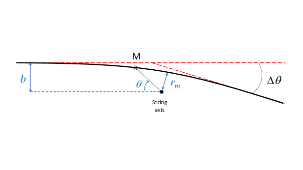
Figure 1: Deviation of a light ray (black thick line) in the presence of a fractional cosmic string.

For light, one defines the impact parameter as (see figure 1)

$$b=\frac{L}{E}=\left(\frac{\alpha r^{\eta}}{\Gamma(1+\eta)}\right)^{2}\frac{{\rm d}\theta}{{\rm d}t}$$ (16)

Light-like geodesics are obtained when ${\rm d}s^{2}=0$. The deviation of light rays due to the string is determined from the formula

$$\Delta\theta = 2\int_{r_{m}}^{+\infty}\frac{{\rm d}\theta}{{\rm d}r}{\rm d}r-\pi=2\int_{r_{m}}^{+\infty}\left(\sqrt{\frac{-g_{rr}g_{tt}b^{2}}{g_{\theta\theta}g_{tt}b^{2}+g_{\theta\theta}^{2}}}\right){\rm d}r-\pi$$ (17)

$$= \frac{R^{2}}{b}\int_{r_{m}}^{+\infty}\frac{{\rm d}r}{r^{\eta}\sqrt{r^{2\eta}-R^{2}}}-\pi$$

with $R^{2}=b^{2}\Gamma(1+\eta)^{2}/\alpha^{2}$. The distance of closest approach $r_{m}=R^{1/\eta}$ is obtained from the condition $\left.\frac{{\rm d}r}{{\rm d}\theta}\right|_{\theta=\theta_{m}}=0$ and $r_{m}=r(\theta_{m})$. Hence the angular deviation becomes

$$\Delta\theta = 2\int_{r_{m}}^{+\infty}\frac{{\rm d}\theta}{{\rm d}r}{\rm d}r-\pi\>=\>2\int_{r_{m}}^{+\infty}\left(\sqrt{\frac{-g_{rr}g_{tt}b^{2}}{g_{\theta\theta}g_{tt}b^{2}+g_{\theta\theta}^{2}}}\right){\rm d}r-\pi$$ (18)

$$= 2\frac{r_{m}^{2\eta}}{b}\int_{r_{m}}^{+\infty}\frac{{\rm d}r}{r^{\eta}\sqrt{r^{2\eta}-r_{m}^{2\eta}}}-\pi$$

$$= 2\frac{r_{m}}{b}\int_{1}^{+\infty}\frac{{\rm d}u}{u^{\eta}\sqrt{u^{2\eta}-1}}-\pi\>=\>\frac{r_{m}}{b}\frac{\sqrt{\pi}}{\eta}\frac{\Gamma(1-1/2\eta)}{\Gamma(3/2-1/2\eta)}-\pi$$

where we used the identity, for $\eta>\frac{1}{2}$

$$I_{\eta}:=\int_{1}^{+\infty}\frac{{\rm d}u}{u^{\eta}\sqrt{u^{2\eta}-1}}=\frac{\sqrt{\pi}}{2\eta}\frac{\Gamma(1-1/2\eta)}{\Gamma(3/2-1/2\eta)}$$ (19)

Interestingly, the validity of this result enforces the condition $\eta>1/2$ which tells us that $\eta=1/2$ needs special consideration. Besides, in the case where $\eta\rightarrow 1$, one recovers the standard result

$$\Delta\theta=\frac{\pi}{\alpha}-\pi.$$ (20)

Ought to the cylindrical symmetry, the lensing effect due to a Nambu-Goto string gives rise to double images of a far-away source, on each side of the string, in contrast with Einstein rings which are expected in the case of spherically symmetric lens. In the case of fractional cosmic strings, one may expect the stretching of the double images as the deviation angle depends on the impact parameter in the form $b^{1/\eta-1}$.

5 Light geodesics

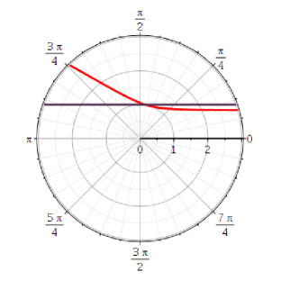
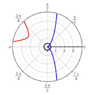
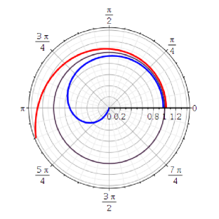
Figure 2: Geodesics $r=r(\theta)=u(\theta)^{1/(1-2\eta)}$ of light in polar coordinates.
Left panel: $\eta=1$. Geodesics for $\alpha=1$ (violet) and for $\alpha=1.2$ (red) are shown. We used $\alpha=b$.
Middle panel: $\eta=3/4$. There is a constant-radius geodesic $r=r_{0}$ (black), and two geodesics which escape to infinity (red & blue). We used ${\cal A}={\cal B}=1$ and $\theta_{0}=0$.
Right panel: $\eta=1/2$. Geodesics are shown for $r(0)<r_{c}$ (blue curve) and $r(0)>r_{c}$ (red curve) and $\frac{{\rm d}r}{{\rm d}\theta}(0)=0$. The limit cycle at $r=r_{c}=1$ is also indicated (see main text).

In analogy to (15), null geodesics are derived by solving the equation

$$\left(\frac{{\rm d}r}{{\rm d}t}\right)^{2}+\frac{\Gamma(1+\eta)^{2}b^{2}}{\alpha^{2}r^{2\eta}}=1$$ (21)

Equivalently, the geodesic orbit $r=r(\theta)$ for light is given by

$$\left(\frac{{\rm d}r}{{\rm d}\theta}\right)^{2}+\left(\frac{\alpha r^{\eta}}{\Gamma(1+\eta)}\right)^{2}=\frac{1}{b^{2}}\left(\frac{\alpha r^{\eta}}{\Gamma(1+\eta)}\right)^{4}$$ (22)

This last equation (22) can be reduced to a simpler form through the ansatz $r=u^{1/\beta}$, where $\beta$ is found from

$$\frac{4\eta}{\beta}-\frac{2}{\beta}+2\stackrel{{\scriptstyle!}}{{=}}0$$ (23)

which eliminates the strongest non-linearity. It follows that $\beta=1-2\eta$ and

$$\left(\frac{{\rm d}u}{{\rm d}\theta}\right)^{2}+\left(\frac{\alpha(1-2\eta)}{\Gamma(1+\eta)}\right)^{2}u^{2\eta/(2\eta-1)}=\frac{(1-2\eta)^{2}}{b^{2}}\frac{\alpha^{4}}{\Gamma^{4}(1+\eta)}\;\;;\;\;\eta\neq\frac{1}{2}$$ (24)

such that for $\eta=1$ this reduces to the equation $\left(\frac{{\rm d}u}{{\rm d}\theta}\right)^{2}+\alpha^{2}u^{2}=\frac{\alpha^{4}}{b^{2}}$. Clearly, for $\alpha=1$ this reproduces a straight line in polar coordinates, as expected. However, for $\alpha\neq 1$ a curved geodesic is obtained, see the left panel of figure 2. This illustrates how straight light rays are bent through a cosmic string.

In general, a reduction of (24) to integrals is straightforward but will involve ill-known special functions. In the simplest case, a reduction of the solutions to elliptic functions is possible. For example, if $\eta=\frac{3}{4}$, from (24) the geodesic curves are solution of the equation

$$\left(\frac{{\rm d}u}{{\rm d}\theta}\right)^{2}+4{\cal A}u^{3}={\cal B}\;\;;\;\;\eta=\frac{3}{4}$$ (25)

with constants ${\cal A},{\cal B}>0$. Eq. (25) is either solved by the constant $u(\theta)=\left(\frac{\cal B}{4{\cal A}}\right)^{1/3}$ or else by a Weierstraß $\wp$ function (see appendix A for details)

$$u(\theta) = -\frac{1}{{\cal A}^{1/3}}\>\wp\left({\cal A}^{1/3}\bigl{(}\theta+\theta_{0}\bigr{)};0,-{\cal B}\right)=\frac{1}{{\cal A}^{1/3}}\>\wp\left({\rm i}{\cal A}^{1/3}\bigl{(}\theta+\theta_{0}\bigr{)};0,+{\cal B}\right)$$ (26)

$$= \left(\frac{\cal B}{\cal A}\right)^{1/3}\wp\left({\rm i}({\cal A}^{2}{\cal B})^{1/6}\bigl{(}\theta+\theta_{0}\bigr{)};0,+1\right)$$

In the middle panel of figure 2, their geometric form in the $(r,\theta)$-plane is illustrated and should be qualitatively similar for all $\frac{1}{2}<\eta<1$. Besides the circle, one class of geodesics $r=r(\theta)=1/u(\theta)^{2}$ passes through the origin which a characteristic cusp (blue curve) and the other class arrives from infinity, passes at the same minimal distance from the origin, and escapes to infinity (red curve). For $\alpha=1$, both geodesics should become straight lines in the $\eta\to 1$ limit and comparison with figure 2 shows how the fractional nature of the parameter $\eta$ impacts on the paths of light rays.

The case $\eta=\frac{1}{2}$ is analysed separately. From (22)

$$\left(\frac{{\rm d}r}{{\rm d}\theta}\right)^{2}+\left(\frac{\alpha}{\Gamma(3/2)}\right)^{2}r=\frac{\alpha^{4}}{b^{2}\Gamma^{4}(3/2)}r^{2}\;\;;\;\;\eta=\frac{1}{2}$$ (27)

Taking a further standard derivative with respect to $\theta$, if $\frac{{\rm d}r}{{\rm d}\theta}\neq 0$ the orbit follows from a Binet-type formula

$$\frac{{\rm d}^{2}r}{{\rm d}\theta^{2}}=\frac{\alpha^{4}}{b^{2}\Gamma^{4}(3/2)}r-\frac{1}{2}\left(\frac{\alpha}{\Gamma(3/2)}\right)^{2}=\frac{\alpha^{4}}{b^{2}\Gamma^{4}(3/2)}\left[r-\frac{b^{2}\Gamma^{2}(3/2)}{2\alpha^{2}}\right]\;\;;\;\;\eta=\frac{1}{2}$$ (28)

First of all, see right panel of figure 2, we see a limit cycle of radius $r_{c}=\frac{b^{2}\Gamma^{2}(3/2)}{2\alpha^{2}}>0$. For radii such that $r<r_{c}$, there is an inward spiral and after a rotation on an angular scale of $\omega^{2}=\left(\frac{2\pi}{\theta_{\rm osc}}\right)^{2}=\frac{\alpha^{4}}{b^{2}\Gamma^{4}(3/2)}$, the radius has shrunk to zero. In other words, in this regime, light cannot escape the gravitational field of the string and gets trapped at the defect core. On the other hand, for $r>r_{c}$, the generic motion is away from the limit cycle, and only for very special initial conditions one might find a convergence to it. The geodesics shown in the right panel of figure 2 for $\eta=\frac{1}{2}$ correspond to half the trajectories shown in the middle panel of figure 2, for $\eta=\frac{3}{4}$. Important differences with respect to the spiralling around the origin can be seen.

6 Concluding remarks

In this work, we determined the metric surrounding a cosmic string in the context of fractional cosmology. Our calculation, based on the Caputo derivative, illustrates how the corresponding time-space geometry depends both on the mass-energy density of the string and on the fractional dimension $\eta$.

Instead of double point-like images of far-away sources, the lensing effects due to a fractional cosmic string are likely to produce stretched double images as the deviation angle depends on the impact parameter in the form $b^{1/\eta-1}$. The light paths are strongly dependent on the fractional parameter, with the case $\eta=1/2$ giving rise to possible trapping effects towards the defect core.

Because the time-space geometry of such defect is no longer that of a cone, one may expect other significant observational signatures. One of them is the Kaiser-Stebbins effect: for a moving Nambu-Goto string, this mechanism predicts the existence of step-like discontinuities in the cosmic microwave background temperature [18]. Up to now, it has not been detected for regular string and a possible extension of the present work could consist in implementing the Kaiser-Stebbins effect for a fractional defect. This will be treated in a forthcoming paper.

Appendix A. On the Weierstraß $\wp$-function

Some background is provided on the elliptic $\wp$-functions, needed in solving (24) and which is taken from [21].

An elliptic function has two complex half-periods $\omega,\omega^{\prime}\in\mathbb{C}$ with ${\rm Im\ }\frac{\omega^{\prime}}{\omega}>0$ and such that $f(z)=f(z+2M\omega+2N\omega^{\prime})$ for $N,M\in\mathbb{Z}$ and $z\in\mathbb{C}$. The special Weierstraß function $\wp=\wp(z;0,1)$ is a solution of the differential equations [22, 23]

$$\frac{{\rm d}^{2}\wp(z)}{{\rm d}z^{2}}+6\wp^{2}(z)=0\;\;;\;\;\left(\frac{{\rm d}\wp(z)}{{\rm d}z}\right)^{2}+4\wp^{3}(z)+1=0$$ (A.1)

and we use the notation $\wp=\wp(z;g_{2},g_{3})$ in terms of the invariants

$$g_{2}=60{\sum_{N,M}}^{\prime}\frac{1}{\bigl{(}2M\omega+2N\omega^{\prime}\bigl{)}^{4}}\;\;,\;\;g_{3}=140{\sum_{N,M}}^{\prime}\frac{1}{\bigl{(}2M\omega+2N\omega^{\prime}\bigl{)}^{6}}$$ (A.2)

where the sums over all pairs of integers $(M,N)$ exclude the pair $(0,0)$. The discriminant $\Delta=g_{2}^{3}-27g_{3}^{2}=-27<0$ in the case at hand. The $\wp$-function belongs to the most simple elliptic functions since it has a single pôle of second order $\wp(z)\sim z^{-2}$ in the fundamental period parallelogram $0\,2\omega\,2\omega+2\omega^{\prime}\ 2\omega^{\prime}$ which for $\Delta<0$ has the form of a rhombus. One has the identities $\wp(z^{*})=\wp(z)^{*}$ and $\wp(z;g_{2},-g_{3})=-\wp({\rm i}z;g_{2};g_{3})$ [21, (18.2.16)] and the scaling $\wp\bigl{(}tz;t^{-4}g_{2},t^{-6}g_{3}\bigr{)}=t^{-2}\wp(z;g_{2},g_{3})$ [21, (18.2.13)]. Hence, along the imaginary axis, $\wp({\rm i}y;0,1)$ is a real-valued and symmetric function of $y$, with period $2\sqrt{3}\omega_{2}\simeq 5.299916$ since $\omega_{2}=\frac{\Gamma(1/3)^{3}}{4\pi}\simeq 1.529954$ in the equi-anharmonic case, defined by $g_{2}=0$ and $g_{3}=1$ [21]. In this case, the two periods are $2\omega,2\omega^{\prime}=\omega_{2}\bigl{(}1\mp{\rm i}\sqrt{3}\bigr{)}$. Finally, as an elliptic function of order 2, $\wp({\rm i}y;0,1)$ has exactly two zeros in the fundamental period parallelogram, which occur at

$$y_{0}^{(\pm,N)}=\pm\frac{2\omega_{2}}{\sqrt{3\,}}+N2\sqrt{3\,}\omega_{2}\simeq\left\{\begin{array}[]{l}1.176639+N5.299916\\ 3.533277+N5.299916\end{array}\right.$$ (A.5)

with $N\in\mathbb{Z}$.

Appendix B. Fractional calculus

A brief summary of results of fractional calculus is given, see e.g. [24, 25, 26] for further details. As a motivation, consider Abel’s integral equation

$$g(x)=\int_{b}^{z}\frac{f(y)\,{\rm d}y}{(x-y)^{\eta}},\quad 0<\eta<1,$$ (B.1)

where $g(x)$ is assumed known. Laplace transformations shows that the requested $f(x)$ is given by

$$f(x)=\frac{\sin\pi\eta}{\pi}\frac{{\rm d}}{{\rm d}x}\int_{b}^{x}\frac{g(y)\,{\rm d}y}{(x-y)^{1-\eta}},\quad 0<\eta<1.$$ (B.2)

Without loss of generality, let from now on $b=0$. The fractional Caputo derivative of order $\eta$, written as ${{}^{c}}D^{\eta}f(x)$, is defined as

$${{}^{c}}D^{\eta}f(x):=\frac{1}{\Gamma(1-\eta)}\int_{0}^{x}\frac{f^{\prime}(y){\rm d}y}{(x-y)^{\eta}}.$$ (B.3)

where $f^{\prime}(x)$ denotes the standard first-order derivative. The Caputo derivative is distinguished from the fractional order Riemann Liouville derivative, defined as

$$^{r}D^{\eta}f(x):=\frac{1}{\Gamma(1-\eta)}\frac{{\rm d}}{{\rm d}x}\int_{0}^{x}\frac{f(y)\,{\rm d}y}{(x-y)^{\eta}}$$ (B.4)

where again $0<\eta<1$. The solution (B.2) can be written as $f(x)=\frac{\sin\bigl{(}\pi\eta\bigr{)}\Gamma(1-\eta)}{\pi}\,{{}^{r}}D^{\eta}g(x)$. Using the Leibniz rule for differentiation, it follows that the two definitions (B.3,B.4) of fractional derivatives are related

$${}^{r}D^{\eta}f(x)={{}^{c}}D^{\eta}f(x)+\frac{f(0)}{\Gamma(1-\eta)x^{\eta}}.$$ (B.5)

In particular, the Caputo derivative of a power function $f(x)=x^{\beta}$ (with $\beta\neq 0$) is

$$^{c}D^{\eta}x^{\beta}=\frac{\Gamma(\beta+1)}{\Gamma(\beta+1-\eta)}x^{\beta-\eta},\quad\beta\neq 0$$ (B.6)

whereas for a constant function (i.e. $\beta=0$), the Caputo definition (B.3) leads to the result

$$^{c}D^{\eta}\,1=0.$$ (B.7)

familiar for a standard derivative. On the other hand, the Riemann-Liouville definition (B.4) rather gives

$${}^{r}D^{\eta}\,1=\frac{1}{\Gamma(1-\eta)}x^{-\eta}.$$ (B.8)

which renders the formulation of initial-value problem in a fractional differential equation difficult. For a linear combination of functions $f(x)=a_{1}f_{1}(x)+f_{2}(x)$, both definitions of the fractional derivative satisfy the linear relation:

$$D^{\eta}f(x)=a_{1}D^{\eta}f_{1}(x)+a_{2}D^{\eta}f_{2}(x).$$ (B.9)

However, neither of them satisfy the semi-group property for iterative derivatives, i.e.

$$D^{\eta_{1}}D^{\eta_{2}}f(x)\neq D^{\eta_{1}+\eta_{2}}f(x).\qquad\eta_{1},\eta_{2}\in(0,1).$$ (B.10)

The property eq. (B.7) motivates our choice of the Caputo fractional derivative in this work. It appears to us as the most suitable to describe the physical scenario of interest. The analysis of fractional calculus, within the context of diffusion equations (for either Riemann-Liouville or Caputo derivatives) is studied in detail in [26].

References

- [1] Jan Ambjørn, Jerzy Jurkiewicz, and Renate Loll. The spectral dimension of the universe is scale-dependent. Physical Review Letters, 95, 171301 (2005) [arxiv:hep-th/0505113].
- [2] Oliver Lauscher and Martin Reuter. Fractal spacetime structure in asymptotically safe gravity. Journal of High Energy Physics 2005(10):050 (2005) [arXiv:hep-th/0508202].
- [3] Leonardo Modesto. Fractal time-space from the area spectrum. Classical and Quantum Gravity 26, 242002 (2009) [arXiv:0812.2214].
- [4] Dario Benedetti. Fractal properties of quantum spacetime. Physical Review Letters 102, 111303 (2009) [arXiv:0811.1396].
- [5] Petr Horava. Spectral dimension of the universe in quantum gravity at a Lifshitz point. Physical Review Letters 102, 161301 (2009) [arXiv:0902.3657].
- [6] Gianluca Calcagni. Multifractional theories: An updated review. Modern Physics Letters A36, 2140006 (2021) [arXiv:2103.06557].
- [7] Laurent Nottale. Fractal space-time and microphysics: towards a theory of scale relativity. World Scientific (Singapour 1993).
- [8] Gianluca Calcagni. Classical and quantum gravity with fractional operators. Classical and Quantum Gravity 38, 165005 (2021) [arXiv:2106.15430].
- [9] Rami Ahmad El-Nabulsi. Fractional derivatives generalization of Einstein’s field equations. Indian Journal of Physics 87, 195 (2013).
- [10] Miguel A. García-Aspeitia, Guillermo Fernández-Anaya, A. Hernández-Almada, Genly Leon, and Juan Magaña. Cosmology under the fractional calculus approach. Monthly Notices of the Royal Astronomical Society 517, 4813 (2022) [arXiv:2207.00878].
- [11] Antonio Di Teodoro and Ernesto Contreras. A vacuum solution of modified Einstein equations based on fractional calculus. The European Physical Journal C83, 1 (2023) [arXiv:2305.15232].
- [12] Rachel Jeannerot, Jonathan Rocher, and Mairi Sakellariadou. How generic is cosmic string formation in supersymmetric grand unified theories. it Physical Review D68, 103514 (2003) [arXiv:hep-ph/0308134].
- [13] Alexander Vilenkin and E. Paul S. Shellard. Cosmic strings and other topological defects. Cambridge University Press (1994).
- [14] Alexander Vilenkin. Gravitational field of vacuum domain walls and strings. Physical Review D23, 852 (1981).
- [15] Sébastien Fumeron and Bertrand Berche. Introduction to topological defects: from liquid crystals to particle physics. European Physical Journal Special Topics, 232, 1813 (2023). [arXiv:2209.07743].
- [16] Peter A. R. Ade, N. Aghanim, C. Armitage-Caplan, M. Arnaud, M. Ashdown, F. Atrio-Barandela, J. Aumont, C. Baccigalupi, A J. Banday, and R. B. et al Barreiro. Planck 2013 results. XXV. searches for cosmic strings and other topological defects. Astronomy & Astrophysics 571, A25 (2014) [arXiv:1303.5085].
- [17] M.A. Fernandez, Simeon Bird, and Yanou Cui. Cosmic filaments from cosmic strings. Physical Review D102, 043509 (2020) [arXiv:2004.13752].
- [18] Nick Kaiser and Albert Stebbins. Microwave anisotropy due to cosmic strings. Nature 310, 391 (1984).
- [19] Simone Blasi, Vedran Brdar, and Kai Schmitz. Has NANOGrav found first evidence for cosmic strings ? Phys. Rev. Lett. 126, 041305 (2021) [arXiv:2009.06607].
- [20] Alexander Vilenkin. Cosmic strings and domain walls. Physics Reports 121, 263 (1985).
- [21] Milton Abramowitz and Irene A. Stegun. Handbook of mathematical functions, Dover (New York 1965).
- [22] Erich Kamke. Differentialgleichungen: Lösungsmethoden und Lösungen I, 9th ed., Teubner (Stuttgart 1977).
- [23] A.D. Polyanin and V.F. Zaitsev. Handbook of Ordinary Differential Equations, 3rd ed., CRC Press (London 2018).
- [24] Richard Herrmann. Fractional calculus: an introduction for physicists, 2nd ed., World Scientific (Singapour 2014).
- [25] I. Podlubny, Fractional differential equations, Academic Press (London 1999).
- [26] Kai Diethelm. The analysis of fractional differential equations, Lecture Notes in Mathematics 2004, Springer (Heidelberg 2010).