Robust Adaptive MPC Using Uncertainty Compensation*

Abstract

This paper presents an uncertainty compensation-based robust adaptive model predictive control (MPC) framework for linear systems with both matched and unmatched nonlinear uncertainties subject to both state and input constraints. In particular, the proposed control framework leverages an ${\mathcal{L}_{1}}$ adaptive controller (${\mathcal{L}_{1}}$AC) to compensate for the matched uncertainties and to provide guaranteed uniform bounds on the error between the states and control inputs of the actual system and those of a nominal i.e., uncertainty-free, system. The performance bounds provided by the ${\mathcal{L}_{1}}$AC are then used to tighten the state and control constraints of the actual system, and a model predictive controller is designed for the nominal system with the tightened constraints. The proposed control framework, which we denote as uncertainty compensation-based MPC (UC-MPC), guarantees constraint satisfaction and achieves improved performance compared with existing methods. Simulation results on a flight control example demonstrate the benefits of the proposed framework.

I Introduction

Real-world systems often require strict adherence to state and/or input constraints stemming from actuator limitations, safety considerations, efficiency requirements, and the need for collision and obstacle avoidance. To deal with systems under constraints, Model Predictive Control (MPC) has emerged as a popular control methodology. MPC optimizes control inputs over a finite time horizon while directly incorporating constraints into the optimization procedure [1, 2]. In addition to the constraints, there are often model uncertainties such as unknown parameters, unmodeled dynamics, and external disturbances, which have to be considered in the control design. MPC has inherent robustness properties to small uncertainties due to the receding-horizon implementation [3]. However, larger uncertainties need to be explicitly treated in the design. Consequently, researchers have explored robust or tube MPC strategies to address uncertainties [4, 5, 6, 7, 8, 9, 10], and most of these works consider bounded disturbances. A summary of several robust MPC approaches can be found in [11]. However, in practical applications, controllers based on robust MPC can perform conservatively and adaptive MPC approaches have also been explored for systems with parametric uncertainties. These approaches typically involve the online identification of a set that is guaranteed to contain the unknown parameters and leverage such a set for robust constraint satisfaction [12, 13, 14, 15]. However, such approaches require a prior known parametric structure for the uncertainties and, moreover, need the parameters to be time-invariant.

Recently, uncertainty compensation based constrained control has also been investigated, which typically involves a control design that estimates and cancels the model uncertainties to force the actual system to behave close to the nominal (uncertainty-free) system. For instance, the authors of [16] integrated an ${\mathcal{L}_{1}}$ adaptive controller (${\mathcal{L}_{1}}$AC)[17] into a reference governor to control systems with time and sate-dependent uncertainties, where the ${\mathcal{L}_{1}}$AC actively compensates for the uncertainties and provides uniform bounds on the error between the states and control inputs of the actual system and a nominal system. Such bounds are then used to tighten the original state and input constraints for robust constraint satisfaction in reference governor design. In [18], the authors integrated an ${\mathcal{L}_{1}}$ adaptive controller with robust MPC to deal with systems subject to unknown parameters and disturbances. In particular, [18] considers the state deviation between the actual system and the nominal system from ${\mathcal{L}_{1}}$AC as a bounded model uncertainty and uses robust MPC to handle it. However, the model uncertainty considered in robust MPC is different from the state deviation bound provided by ${\mathcal{L}_{1}}$AC and [18] does not account for the tightening of input constraint resulting from the additional adaptive control input introduced by ${\mathcal{L}_{1}}$AC. Additionally, both [16] and [18] only consider matched uncertainties, i.e., uncertainties injected into the system through the same channels as control inputs.

Contribution: This paper presents a robust adaptive MPC framework based on uncertainty compensation, which we term as UC-MPC, for linear systems with nonlinear and time-varying uncertainties that can contain both matched and unmatched components. Our framework leverages an ${\mathcal{L}_{1}}$AC to estimate and compensate for the matched uncertainties, and to guarantee uniform bounds on the error between states and inputs of the actual system and those of a nominal (i.e., uncertainty-free) closed-loop system. Such bounds are then used to tighten the original constraints. The tightened constraints are leveraged in the design of MPC for the nominal system, which guarantees robust constraint satisfaction of the actual system in the presence of uncertainties. To validate the effectiveness of our framework, we conduct simulations using a flight control example.

The proposed UC-MPC has the following features:

• In addition to the enforcement of the constraints, UC-MPC improves the tracking performance compared with existing robust or tube MPC solutions [4, 5, 6, 7, 8, 9, 10], due to the active uncertainty compensation.

• UC-MPC handles a broad class of uncertainties that can be time-varying and state-dependent without a parametric structure, while existing adaptive MPC approaches[12, 13, 14, 15] typically handle parametric uncertainties only.

• UC-MPC can also handle unmatched disturbances while existing uncertainty compensation-based constrained control only considers matched uncertainties [18, 16].

Notations: In this paper, we use $\mathbb{R}$, $\mathbb{R}_{+}$ and $\mathbb{Z}_{+}$ to denote the set of real, non-negative real, and non-negative integer numbers, respectively. $\mathbb{R}^{n}$ and $\mathbb{R}^{m\times n}$ represent the $n$-dimensional real vector space and the set of real $m$ by $n$ matrices, respectively. $\mathbb{Z}_{i}$ and $\mathbb{Z}_{1}^{n}$ denote the integer sets $\{i,i+1,\cdots\}$ and $\{1,2,\cdots,n\}$, respectively. $I_{n}$ denotes a size $n$ identity matrix, and $0$ is a zero matrix of a compatible dimension. $\left\lVert\cdot\right\rVert$ and $\left\lVert\cdot\right\rVert_{\infty}$ represent the $2$-norm and $\infty$-norm of a vector or a matrix, respectively. The $\mathcal{L}_{\infty}$- and truncated $\mathcal{L}_{\infty}$-norm of a function $x:\mathbb{R}_{+}\rightarrow\mathbb{R}^{n}$ are defined as $\left\lVert x\right\rVert_{\mathcal{L}_{\infty}}\triangleq\sup_{t\geq 0}\left\lVert x(t)\right\rVert_{\infty}$ and $\left\lVert x\right\rVert_{\mathcal{L}_{\infty}^{[0,T]}}\triangleq\sup_{0\leq t\leq T}\left\lVert x(t)\right\rVert_{\infty}$, respectively. The Laplace transform of a function $x(t)$ is denoted by $x(s)\triangleq\mathfrak{L}[x(t)]$. Given a vector $x$, $x_{i}$ denotes the $i$th element of $x$. For positive scalar $\rho$, $\Omega(\rho)\triangleq\{z\in\mathbb{R}^{n}:\left\lVert z\right\rVert_{\infty}\leq\rho\}$ represents a high dimensional ball set of radius $\rho$ which centers at the origin with a compatible dimension $n$. For a high-dimensional set $\mathcal{X}$, the interior of $\mathcal{X}$ is denoted by $\textup{int}(\mathcal{X})$ and the projection of $\mathcal{X}$ onto the $i$th coordinate is represented by $\mathcal{X}_{i}$. For given sets $\mathcal{X},{\mathcal{Y}}\subset\mathbb{R}^{n}$, $\mathcal{X}\oplus{\mathcal{Y}}\triangleq\{x+y:x\in\mathcal{X},y\in{\mathcal{Y}}\}$ is the Minkowski set sum and $\mathcal{X}\ominus{\mathcal{Y}}\triangleq\{z:z+y\in\mathcal{X},\forall y\in{\mathcal{Y}}\}$ is the Pontryagin set difference.

II Problem Statement

Consider a linear system with uncertainties represented by

$$\left\{\begin{aligned} \dot{x}(t)&=Ax(t)+B(u(t)+f(t,x(t)))+B_{u}w(t),\hfill\\ y(t)&=Cx(t),\ x(0)=x_{0},\\ \end{aligned}\right.$$ (1)

where $x(t)\in\mathbb{R}^{n}$, $u(t)\in\mathbb{R}^{m}$ and $y(t)\in\mathbb{R}^{m}$ represent the state, input, and output vectors, respectively, $x_{0}\in\mathbb{R}^{n}$ is the initial state, and matrices $A$, $B$, $B_{u}$, and $C$ are known with compatible dimensions. $B$ has full column rank, and $B_{u}$ is a matrix such that $\textup{rank}[B\ B_{u}]=n$ and $B_{u}^{T}B=0$. Moreover, $f(t,x(t))\in\mathbb{R}^{m}$ represents the matched uncertainty dependent on both time and states, and $w(t)\in\mathbb{R}$ denotes the unmatched uncertainty.

Assumption 1.

Given a compact set ${\mathcal{Z}}$, there exist positive constants $L_{f_{j},{\mathcal{Z}}}$, $l_{f_{j},{\mathcal{Z}}}$, and $b_{f_{j},{\mathcal{Z}}}$ ($j\in\mathbb{Z}_{1}^{m}$) such that for any $x,z\in{\mathcal{Z}}$ and $t,\tau\geq 0$, the following inequalities hold for all $j\in\mathbb{Z}_{1}^{m}$:

$$\left\lvert f_{j}(t,x)-f_{j}(\tau,z)\right\rvert \!\leq\!L_{f_{j},{\mathcal{Z}}}\left\lVert x-z\right\rVert_{\infty}\!+\!l_{f_{j},{\mathcal{Z}}}\left\lvert t-\tau\right\rvert,$$ (2a)

$$\left\lvert f_{j}(t,x)\right\rvert \leq b_{f_{j},{\mathcal{Z}}},$$ (2b)

where $f_{j}(t,x)$ denotes the $i$th element of $f(t,x)$. In addition, there exist a positive constant $b_{w}$ such that for any $t\geq 0$, we have:

$$\left\lVert w(t)\right\rVert_{\infty}\leq b_{w}.$$ (3)

Remark 1.

The function $f(t,x)$ represents the matched uncertainty that can be directly canceled using control inputs. On the other hand, $w(t)$ denotes the unmatched uncertainty that cannot be directly canceled. Since the proposed solution needs to be robust against the unmatched uncertainty, we restrict $w(t)$ to be bounded and state-independent to simplify the derivation. It is possible to slightly extend the results to allow $w(t)$ to be state-dependent.

Based on Assumption 1, it follows that for any $x,z\in{\mathcal{Z}}$ and $t,\tau\geq 0$, we have

$$\left\lVert f(t,x)-f(\tau,z)\right\rVert_{\infty} \!\leq\!{L_{f,{\mathcal{Z}}}}\left\lVert x-z\right\rVert_{\infty}\!+\!l_{f,{\mathcal{Z}}}\left\lvert t-\tau\right\rvert,$$ (4a)

$$\left\lVert f(t,x)\right\rVert_{\infty} \leq{b_{f,{\mathcal{Z}}}},$$ (4b)

$$\left\lVert w(t)\right\rVert_{\infty} \leq b_{w},$$ (4c)

where

$$L_{f,{\mathcal{Z}}} =\max_{j\in\mathbb{Z}_{1}^{m}}L_{f_{j},{\mathcal{Z}}},\;l_{f,{\mathcal{Z}}}=\max_{j\in\mathbb{Z}_{1}^{m}}l_{f_{j},{\mathcal{Z}}},$$

$$b_{f,{\mathcal{Z}}} =\max_{j\in\mathbb{Z}_{1}^{m}}b_{f_{j},{\mathcal{Z}}}.$$ (5)

Remark 2.

We specifically make assumptions on $f_{j}(t,x)$ instead of on $f(t,x)$ as in Section II in order to derive an individual bound on each state and on each adaptive input (see Section IV for details).

Given the system 1, the goal of this paper is to design an MPC scheme with active uncertainty compensation to achieve desired performance while satisfying the following state and control constraints:

$$\begin{gathered}x(t)\in\mathcal{X},\quad u(t)\in\mathcal{U},\quad\forall t\geq 0,\hfill\end{gathered}$$ (6)

where $\mathcal{X}\subset\mathbb{R}^{n}$ and ${\mathcal{U}}\subset\mathbb{R}^{m}$ are pre-specified convex and compact sets including the origin.

III Overview of the UC-MPC Framework

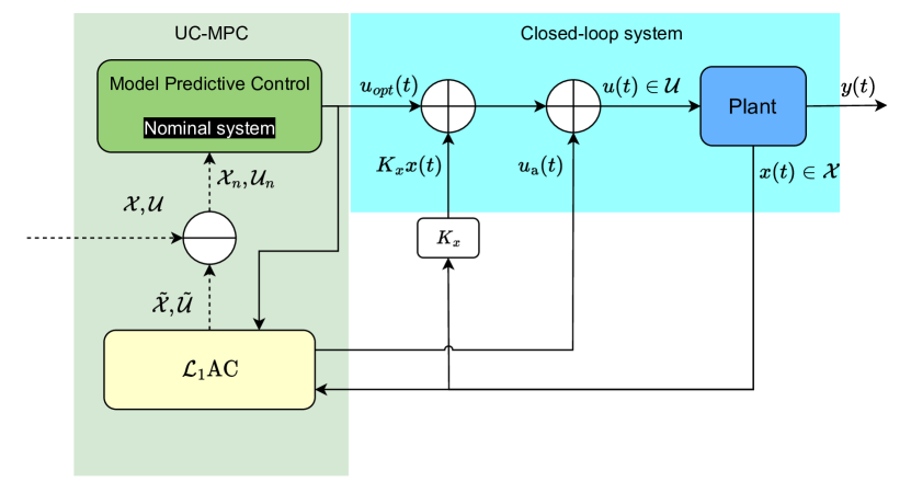
Figure 1: Diagram of the proposed UC-MPC framework

The schematic diagram of the proposed UC-MPC is shown in Fig. 1, which includes a feedback control law $K_{x}x(t)$, an ${\mathcal{L}_{1}}$AC to generate $u_{a}(t)$, and an MPC design for the nominal system with tightened constraints $\mathcal{X}_{\textup{n}}$ and ${\mathcal{U}}_{\textup{n}}$ to generate $u_{\text{opt}}(t)$. In the presence of the uncertainties $f(t,x)$ and $w(t)$, we leverage an ${\mathcal{L}_{1}}$AC to generate $u_{a}(t)$ to compensate for the matched uncertainty and to force the actual system to behave close to a nominal (i.e., uncertainty-free) system [17]. The feedback control law $K_{x}x(t)$ ensures that $A+BK_{x}$ is Hurwitz. Thus, the overall control law for system 1 can be represented as:

$$u(t)=K_{x}x(t)+u_{\text{opt}}(t)+u_{a}(t).$$ (7)

With 7, we can reformulate the system 1 as

$$\left\{\begin{aligned} \!\dot{x}(t)\!&=\!{A_{m}}x(t)\!+\!Bu_{\text{opt}}(t)\!+\!B(u_{\textup{a}}(t)\!+\!f(t,\!x(t)\!)\!)\!+\!B_{u}w(t)\\ \!y(t)&=Cx(t),\ x(0)=x_{0},\end{aligned}\right.$$ (8)

where ${A_{m}}\triangleq A+B{K_{x}}$ is a Hurwitz matrix. In Section IV, we will show that the existence of ${\mathcal{L}_{1}}$AC provides uniform bounds on the errors between the states and control inputs of the real plant 8 and those of the nominal system represented by

$$\left\{\begin{aligned} \dot{x}_{\textup{n}}(t)&={A_{m}}x_{\textup{n}}(t)+Bu_{\text{opt}}(t),\ x_{\textup{n}}(0)=x_{0},\hfill\\ u_{\textup{n}}(t)&=K_{x}x_{\textup{n}}(t)+u_{\text{opt}}(t),\end{aligned}\right.$$ (9)

where $x_{\textup{n}}$ and $u_{\textup{n}}$ are the vectors of nominal states and inputs. Using the uniform bounds from ${\mathcal{L}_{1}}$AC, we design an MPC for the nominal system with tightened constraints. In particular, from ${\mathcal{L}_{1}}$AC, we achieve

$$x(t)-x_{\textup{n}}(t)\in\tilde{\mathcal{X}},\quad u(t)-u_{\textup{n}}(t)\in\tilde{\mathcal{U}},\quad\forall t\geq 0,$$ (10)

where $u(t)$ is defined in 7 and $u_{\textup{n}}(t)$ is given in 9, and $\tilde{\mathcal{X}}$ and $\tilde{\mathcal{U}}$ are some pre-computed hyperrectangular sets calculated from the range of $f(t,x)$ and $w(t)$ and the design of ${\mathcal{L}_{1}}$AC. Given the state and control input constraints of the real plant $\mathcal{X}$ and $\mathcal{U}$ in 6, the tightened constraints for the nominal system 9 are represented by

$$\mathcal{X}_{\textup{n}}\triangleq\mathcal{X}\ominus\tilde{\mathcal{X}},\quad{\mathcal{U}}_{\textup{n}}\triangleq{\mathcal{U}}\ominus\tilde{\mathcal{U}}.$$ (11)

IV ${\mathcal{L}_{1}}$AC With Uniform Performance Bounds

We now present the uniform performance bounds provided by an ${\mathcal{L}_{1}}$AC on the errors between the states and control inputs of the real plant 8 and those of the nominal system 9. A preliminary result is presented in [16], in which the authors considered only matched uncertainties. In this paper, we extend the result to systems with both matched uncertainty $f(t,x(t))$ and unmatched uncertainty $w(t)$.

An ${\mathcal{L}_{1}}$AC usually includes three elements: a state predictor, an estimation law, and a low-pass filter. The inclusion of a low-pass filter ${\mathcal{C}}(s)$ (with DC gain ${\mathcal{C}}(0)=I_{m}$) decouples the estimation loop from the control loop, which enables fast adaptation without sacrificing the robustness [17]. The low-pass filter ${\mathcal{C}}(s)$ can be designed as a first-order transfer function matrix

$${\mathcal{C}}(s)=\textup{diag}({\mathcal{C}}_{1}(s),\dots,{\mathcal{C}}_{m}(s)),\ {\mathcal{C}}_{j}(s)\triangleq\frac{k_{f}^{j}}{(s+k_{f}^{j})},$$ (12)

where $k^{j}_{f}$ ($j\in\mathbb{Z}_{1}^{m}$) represents the bandwidth for the $j$th input channel. In order to ensure stability, given the compact set $\mathcal{X}_{0}$, the filter ${\mathcal{C}}(s)$ defined in 12 needs to ensure that there exists a positive constant $\rho_{r}$ and a (small) positive constant $\gamma_{1}$ such that

$$\left\lVert\mathcal{G}_{xm}(s)\right\rVert_{\mathcal{L}_{1}}b_{f,\mathcal{X}_{r}} <\rho_{r}-\left\lVert\mathcal{H}_{xm}(s)\right\rVert_{\mathcal{L}_{1}}\left\lVert u_{\text{opt}}\right\rVert_{\mathcal{L}_{\infty}}$$

$$-\left\lVert\mathcal{H}_{xu}(s)\right\rVert_{\mathcal{L}_{1}}b_{w}-\rho_{\textup{in}},$$ (13a)

$$\left\lVert\mathcal{G}_{xm}(s)\right\rVert_{\mathcal{L}_{1}}L_{f,\mathcal{X}_{a}} <1,$$ (13b)

where

$$\rho \triangleq\rho_{r}+\gamma_{1},$$ (14)

$$\mathcal{X}_{r} \triangleq\Omega(\rho_{r}),\ \mathcal{X}_{a}\triangleq\Omega(\rho).$$ (15)

$$\mathcal{H}_{xm}(s) \triangleq\!(sI_{n}\!-\!A_{m})^{-1}\!B,$$ (16)

$$\mathcal{H}_{xu}(s) \triangleq\!(sI_{n}\!-\!A_{m})^{-1}\!B_{u},$$ (17)

$$\mathcal{G}_{xm}(s) \triangleq\!\mathcal{H}_{xm}(s)(I_{m}-{\mathcal{C}}(s)),$$ (18)

$$\rho_{\textup{in}} \triangleq\left\lVert s(sI_{n}-A_{m})^{-1}\right\rVert_{\mathcal{L}_{1}}\max_{x_{0}\in\mathcal{X}_{0}}\left\lVert x_{0}\right\rVert_{\infty}.$$ (19)

Also, we define $x_{\textup{in}}(t)$ as the state of the system $\dot{x}_{\textup{in}}(t)=A_{m}x_{\textup{in}}(t),\ x_{\textup{in}}(0)=x_{0},$ and we have $x_{\textup{in}}(s)\triangleq(sI_{n}-A_{m})^{-1}x_{0}$.

For the real system 8, the state predictor is defined as

$$\dot{\hat{x}}(t)\!=\!A_{m}x(t)\!+\!Bu_{\text{opt}}(t)\!+\!Bu_{\textup{a}}(t)\!+\!\hat{\sigma}(t)\!+\!A_{e}\tilde{x}(t),$$ (20)

where $\hat{x}(0)=x_{0}$, $\tilde{x}(t)=\hat{x}(t)-x(t)$ is the prediction error, $A_{e}$ is a custom Hurwitz matrix, and $\hat{\sigma}(t)$ is the estimate of the lumped uncertainty, $Bf(t,x)+B_{u}w(t)$. The estimate $\hat{\sigma}(t)$ is updated according to the following piecewise-constant estimation law (similar to that in [17, Section 3.3]):

$$\left\{\begin{aligned} &\hat{\sigma}(t)&&=\hat{\sigma}(iT),\quad t\in[iT,(i+1)T),\\ &\hat{\sigma}(iT)&&=-\Phi^{-1}(T)e^{A_{e}T}\tilde{x}(iT),\end{aligned}\right.$$ (21)

where $T$ is the estimation sampling time, and $\Phi(T)\triangleq A_{e}^{-1}\left(e^{A_{e}T}\!-I_{n}\right)$. The control law of the adaptive controller is given by

$$u_{\textup{a}}(s)=-{\mathcal{C}}(s)\mathfrak{L}\left[B^{\dagger}\hat{\sigma}(t)\right],$$ (22)

where $B^{\dagger}=(B^{T}B)^{-1}B^{T}$ is the pseudo-inverse of $B$. The control law 22 tries to cancel the estimate of the matched uncertainty $f(t,x(t))$ within the bandwidth of the filter ${\mathcal{C}}(s)$.

Now we define some constants below for future reference:

$$\bar{\alpha}_{0}(T)\triangleq \int_{0}^{T}\left\lVert e^{A_{e}(T-\tau)}B\right\rVert_{\infty}d\tau,$$ (23a)

$$\bar{\alpha}_{1}(T)\triangleq \int_{0}^{T}\left\lVert e^{A_{e}(T-\tau)}B_{u}\right\rVert_{\infty}d\tau,$$ (23b)

$$\bar{\alpha}_{2}(T)\triangleq \max_{t\in[0,T]}\left\lVert e^{A_{e}t}\right\rVert_{\infty},$$ (23c)

$$\bar{\alpha}_{3}(T)\triangleq \max_{t\in[0,T]}\int_{0}^{t}\left\lVert e^{A_{e}(t-\tau)}\Phi^{-1}(T)e^{A_{e}T}\right\rVert_{\infty}d\tau,$$ (23d)

$$\gamma_{0}(T)\triangleq (b_{f,\mathcal{X}_{a}}\bar{\alpha}_{0}(T)\!+\!\bar{\alpha}_{1}(T)b_{w})\!(\bar{\alpha}_{2}(T)\!+\!\bar{\alpha}_{3}(T)\!+\!1\!)\!$$ (23e)

$$\rho_{ur}\triangleq \left\lVert{\mathcal{C}}(s)\right\rVert_{\mathcal{L}_{1}}b_{f,\mathcal{X}_{r}},$$ (23f)

$$\gamma_{2}\triangleq \left\lVert{\mathcal{C}}(s)\right\rVert_{\mathcal{L}_{1}}\!L_{f,\mathcal{X}_{a}}\gamma_{1}\!+\!\left\lVert{\mathcal{C}}(s)B^{\dagger}(sI_{n}\!-\!A_{e})\right\rVert_{\mathcal{L}_{1}}\!\gamma_{0}(T),$$ (23g)

$$\rho_{u_{\textup{a}}}\triangleq \rho_{ur}+\gamma_{2},$$ (23h)

where $\gamma_{1}$ is introduced in 14. Based on the Taylor series expansion of $e^{A_{e}T}$, we have $\lim_{T\rightarrow 0}\int_{0}^{T}\left\lVert\Phi^{-1}(T)\right\rVert_{\infty}d\tau$ is bounded, which further implies that $\lim_{T\rightarrow 0}\bar{\alpha}_{3}(T)$ is bounded. Since $\lim_{T\rightarrow 0}\bar{\alpha}_{0}(T)=0$, $\lim_{T\rightarrow 0}\bar{\alpha}_{1}(T)=0$, $\lim_{T\rightarrow 0}\bar{\alpha}_{2}(T)=0$, $b_{f,\mathcal{X}_{a}}$ is bounded for a compact set $\mathcal{X}_{a}$, $b_{w}$ is bounded, and $\lim_{T\rightarrow 0}\bar{\alpha}_{3}(T)$ is bounded, we have

$$\lim_{T\rightarrow 0}\gamma_{0}(T)=0.$$ (24)

Considering 24 and 13b, it is always feasible to find a small enough $T>0$ such that

$$\frac{\left\lVert\mathcal{H}_{xm}(s){\mathcal{C}}(s)B^{\dagger}(sI_{n}-A_{e})\right\rVert_{\mathcal{L}_{1}}}{1-\left\lVert\mathcal{G}_{xm}(s)\right\rVert_{\mathcal{L}_{1}}L_{f,\mathcal{X}_{a}}}\gamma_{0}(T)<\gamma_{1},$$ (25)

where $\mathcal{X}_{a}$ is defined in 15 and $B^{\dagger}$ is the pseudo-inverse of $B$.

Following the convention of an ${\mathcal{L}_{1}}$AC[17], we introduce the following reference system for performance analysis:

$$\dot{x}_{\textup{r}}(t) \!=\!{A_{m}}x_{\textup{r}}(t)\!\!+\!\!{B}u_{\text{opt}}(t)\!\!+\!\!B({u_{\textup{r}}}(t)\!\!+\!\!f(t,\!x_{\textup{r}}(t)))\!\!+\!\!B_{u}w(t),\hfill$$

$${u_{\textup{r}}}(s) \!=\!-{\mathcal{C}}(s)\mathfrak{L}\left[f(t,x_{\textup{r}}(t))\right],\quad x_{\textup{r}}(0)\!=\!x_{0},$$ (26)

Lemma 1.

Given the uncertain system 8 subject to Assumption 1 and the reference system 26 subject to the conditions 13b and 13a with a constant $\gamma_{1}>0$, with the ${\mathcal{L}_{1}}$AC defined via 20, 21 and 22 subject to the sample time constraint 25, we have

$$\left\lVert x\right\rVert_{\mathcal{L}_{\infty}} \leq\rho,$$ (27a)

$$\left\lVert u_{\textup{a}}\right\rVert_{\mathcal{L}_{\infty}} \leq\rho_{u_{\textup{a}}},$$ (27b)

$$\left\lVert x_{\textup{r}}-x\right\rVert_{\mathcal{L}_{\infty}} \leq\gamma_{1},$$ (27c)

$$\left\lVert u_{\textup{r}}-u_{\textup{a}}\right\rVert_{\mathcal{L}_{\infty}} \leq\gamma_{2},$$ (27d)

where $\rho$, $\rho_{u_{\textup{a}}}$, and $\gamma_{2}$ are defined in 14, 23h, 23g, respectively.

Lemma 2.

Given the reference system 26 and the nominal system 9, subject to Assumption 1, and the condition 13a, we have

$${\left\|{{x_{\textup{r}}}-x_{\textup{n}}}\right\|_{{\mathcal{L}}{{}_{\infty}}}} \leq\left\lVert\mathcal{G}_{xm}\right\rVert_{\mathcal{L}_{1}}b_{f,\mathcal{X}_{r}}+\left\lVert\mathcal{H}_{xu}\right\rVert_{\mathcal{L}_{1}}b_{w}.$$ (28)

Lemma 1 and Lemma 2 are relatively straightforward extensions of [16, Theorem 1 and Lemma 5] with the consideration of the unmatched uncertainty $w(t)$. The proofs can be obtained by extending the proofs of [16, Theorem 1 and Lemma 5] and are included in the appendix.

The previous results provide uniform error bounds as represented by the vector-$\infty$ norm, which always leads to the same bound for all the states, $x_{i}-x_{\textup{n},i}(t)$ ($i\in\mathbb{Z}_{1}^{n}$), or all the adaptive inputs, $u_{\textup{a},j}$ ($j\in\mathbb{Z}_{1}^{m}$). The use of vector-$\infty$ norms may lead to conservative bounds given some states or adaptive inputs, making it impossible to satisfy the constraints 6 or leading to significantly tightened constraints for the MPC design. Thus, an individual bound for each $x_{i}(t)-x_{\textup{r},i}(t)$ is preferred. To derive the individual bounds for each $i\in\mathbb{Z}_{1}^{n}$, we follow [16] to introduce the following coordinate transformations for the reference system 26 and the nominal system 9:

$$\left\{\begin{aligned} \check{x}_{\textup{r}}&=\mathrm{T}_{x}^{i}x_{\textup{r}},\quad\check{x}_{\textup{n}}=\mathrm{T}_{x}^{i}x_{\textup{n}},\\ \check{A}_{m}^{i}&=\mathrm{T}_{x}^{i}A_{m}(\mathrm{T}_{x}^{i})^{-1},\\ \check{B}^{i}&=\mathrm{T}_{x}^{i}B,\quad\check{B}^{i}_{u}=\mathrm{T}_{x}^{i}B_{u},\end{aligned}\right.$$ (29)

where $\mathrm{T}_{x}^{i}\!>\!0$ is a diagonal matrix that satisfies

$$\mathrm{T}_{x}^{i}[i] =1,\ 0<\mathrm{T}_{x}^{i}[k]\leq 1,\ \forall k\neq i,$$ (30)

and $\mathrm{T}_{x}^{i}[k]$ is the $k$th diagonal element. With the transformation 29, the reference system 26 is transformed into

$$\dot{\check{x}}_{\textup{r}}(t) \!=\!\check{A}_{m}^{i}\check{x}_{\textup{r}}(t)\!\!+\!\!\check{B}^{i}u_{\text{opt}}(t)\!\!+\!\!\check{B}^{i}(u_{\textup{r}}(t)\!\!+\!\!\check{f}(t,\check{x}_{\textup{r}}(t)\!)\!)\!+\!\check{B}_{u}^{i}w(t),$$

$${u_{\textup{r}}}(s) \!=\!-{\mathcal{C}}(s)\mathfrak{L}\left[\check{f}(t,\check{x}_{\textup{r}}(t))\right],\ \check{x}(0)\!=\!\mathrm{T}_{x}^{i}x_{0},$$ (31)

where

$$\check{f}(t,\check{x}_{\textup{r}}(t))=f(t,x_{\textup{r}}(t)))=f(t,(\mathrm{T}_{x}^{i})^{-1}\check{x}_{\textup{r}}(t))).$$ (32)

Given a set ${\mathcal{Z}}$, define

$$\check{\mathcal{Z}}\triangleq\{\check{z}\in\mathbb{R}^{n}:(\mathrm{T}_{x}^{i})^{-1}\check{z}\in{\mathcal{Z}}\}.$$ (33)

For the transformed reference system 31, we have

$$\mathcal{H}_{\check{x}m}^{i}(s) \triangleq(sI_{n}\!-\!\check{A}_{m}^{i})^{-1}\!\check{B}^{i}=\mathrm{T}_{x}^{i}\mathcal{H}_{xm}(s),$$ (34a)

$$\mathcal{H}_{\check{x}u}^{i}(s) \triangleq(sI_{n}\!-\!\check{A}_{m}^{i})^{-1}\!\check{B}^{i}_{u}=\mathrm{T}_{x}^{i}\mathcal{H}_{xu}(s),$$ (34b)

$$\mathcal{G}_{\check{x}m}^{i}(s) \triangleq\mathcal{H}_{\check{x}m}^{i}(s)(I_{m}-{\mathcal{C}}(s))=\mathrm{T}_{x}^{i}\mathcal{G}_{xm}(s),$$ (34c)

where $\mathcal{H}_{xm},~{}\mathcal{H}_{xu},~{}\mathcal{G}_{xm}$ are defined in 16, 17 and 18. By applying the transformation 29 to the nominal system 9, we obtain

$$\left\{\begin{aligned} \dot{\check{x}}_{\textup{n}}(t)&=\check{A}_{m}^{i}{\check{x}}_{\textup{n}}(t)+\check{B}^{i}u_{\text{opt}}(t),\ {\check{x}}_{\textup{n}}(0)\!=\!\mathrm{T}_{x}^{i}x_{0},\\ \check{y}_{\text{n}}(t)&=\check{C}{\check{x}}_{\textup{n}}(t).\end{aligned}\right.$$ (35)

Letting ${\check{x}}_{\textup{in}}(t)$ be the state of the system $\dot{\check{x}}_{\textup{in}}(t)=\check{A}_{m}^{i}{\check{x}}_{\textup{in}}(t)$ with ${\check{x}}_{\textup{in}}(0)=\check{x}_{\textup{n}}(0)=\mathrm{T}_{x}^{i}x_{0}$, we have ${\check{x}}_{\textup{in}}(s)\triangleq(sI_{n}-\check{A}_{m}^{i})^{-1}{\check{x}}_{\textup{in}}(0)=\mathrm{T}_{x}^{i}(sI_{n}-A_{m})^{-1}x_{0}$. Define

$$\check{\rho}_{\textup{in}}^{i}\triangleq\left\lVert s\mathrm{T}_{x}^{i}(sI_{n}-A_{m})^{-1}\right\rVert_{\mathcal{L}_{1}}\max_{x_{0}\in\mathcal{X}_{0}}\left\lVert x_{0}\right\rVert_{\infty}.$$ (36)

Similar to 13a, for the transformed reference system 31, given any positive constant $\gamma_{1}$, the lowpass filter design now needs to satisfy:

$$\left\lVert\mathcal{G}_{\check{x}m}^{i}(s)\right\rVert_{\mathcal{L}_{1}}b_{\check{f},\check{\mathcal{X}}_{r}} <\check{\rho}_{r}^{i}-\left\lVert\mathcal{H}_{\check{x}v}^{i}(s)\right\rVert_{\mathcal{L}_{1}}\left\lVert u_{\text{opt}}\right\rVert_{\mathcal{L}_{\infty}}$$

$$-\left\lVert\mathcal{H}_{\check{x}u}^{i}(s)\right\rVert_{\mathcal{L}_{1}}b_{w}-\check{\rho}_{\textup{in}}^{i},$$ (37)

where $\mathcal{X}_{r}$ is defined in 15 and $\check{\mathcal{X}}_{r}$ is defined according to 33, and $\check{\rho}_{r}^{i}$ is a positive constant to be determined.

Lemma 3.

Consider the reference system 26 subject to Assumption 1, the nominal system 9, the transformed reference system 31 and transformed nominal system 35 obtained by applying 29 with any $\mathrm{T}_{x}^{i}$ satisfying 30. Suppose that 13a holds with some constants $\rho_{r}$ and $\left\lVert u_{\text{opt}}\right\rVert_{\mathcal{L}_{\infty}}$. Then, there exists a constant $\check{\rho}_{r}^{i}\leq\rho_{r}$ such that 37 holds with the same $\left\lVert u_{\text{opt}}\right\rVert_{\mathcal{L}_{\infty}}$. Furthermore, $\forall t\geq 0$,

$$\left\lvert x_{\textup{r},i}(t)\right\rvert \leq\check{\rho}_{r}^{i},$$ (38)

$$\left\lvert x_{\textup{r,i}}(t)-x_{\textup{n},i}(t)\right\rvert \leq\left\lVert\mathcal{G}_{\check{x}m}(s)\right\rVert_{\mathcal{L}_{1}}b_{f,\mathcal{X}_{r}}\!+\!\left\lVert\mathcal{H}_{\check{x}u}\right\rVert_{\mathcal{L}_{1}}b_{w},$$ (39)

where we re-define

$$\mathcal{X}_{r}\triangleq\left\{z\in\mathbb{R}^{n}:\left\lvert z_{i}\right\rvert\leq\check{\rho}_{r}^{i},i\in\mathbb{Z}_{1}^{n}\right\}.$$ (40)

Lemma 4.

Consider the uncertain system 8 subject to Assumption 1, the nominal system 9, and the ${\mathcal{L}_{1}}$AC defined via 20, 21 and 22 subject to the conditions 13b and 13a with constants $\rho_{r}$ and $\gamma_{1}>0$ and the sample time constraint 25. Suppose that for each $i\in\mathbb{Z}_{1}^{n}$, 37 holds with a constant $\check{\rho}_{r}^{i}$ for the transformed reference system 31 obtained by applying 29. Then, $\forall t\geq 0$, we have

$${x(t)-x_{\textup{n}}(t)}\!\in\!\tilde{\mathcal{X}}\! \triangleq\!\left\{z\!\in\!\mathbb{R}^{n}\!:\!\left\lvert z_{i}\right\rvert\!\leq\!\tilde{\rho}^{i},\ i\in\mathbb{Z}_{1}^{n}\right\}\!,\$$ (41a)

$${u_{\textup{a}}(t)}\!\in\!{\mathcal{U}}_{\textup{a}}\! \triangleq\!\left\{z\!\in\!\mathbb{R}^{m}\!:\!\left\lvert z_{j}\right\rvert\!\leq\!\rho_{u_{\textup{a}}}^{j},\ \!j\!\in\!\mathbb{Z}_{1}^{m}\right\}\!,$$ (41b)

$$u(t)-u_{\textup{n}}(t)\!\in\!\tilde{\mathcal{U}}\! \triangleq\!\left\{z\!\in\!\mathbb{R}^{m}\!:\!\left\lvert z_{j}\right\rvert\!\leq\!\tilde{\rho}_{u}^{j},\ j\!\in\!\mathbb{Z}_{1}^{m}\right\}\!,$$ (41c)

where

$$\rho^{i}\!\triangleq\!\check{\rho}_{r}^{i}\!+\!\gamma_{1},\tilde{\rho}^{i}\!\triangleq\!\left\lVert\mathcal{G}_{\check{x}m}^{i}(s)\right\rVert_{\mathcal{L}_{1}}\!\!b_{f,\mathcal{X}_{r}}\!+\!\left\lVert\mathcal{H}^{i}_{\check{x}u}\right\rVert_{\mathcal{L}_{1}}\!\!b_{w}+\!\gamma_{1},\!$$ (42a)

$$\rho_{u_{\textup{a}}}^{j}\!\triangleq\!\left\lVert{\mathcal{C}}_{j}(s)\right\rVert_{\mathcal{L}_{1}}b_{f_{j},\mathcal{X}_{r}}\!+\!\gamma_{2},\!\tilde{\rho}_{u}^{j}\!\triangleq\!\rho_{u_{\textup{a}}}^{j}\!+\!\sum_{i=1}^{n}\left\lvert K_{x}[j,i]\right\rvert\tilde{\rho}^{i}$$ (42b)

with $\mathcal{X}_{r}$ defined in 40, and $C[j,i]$ denoting the $(j,i)$ element of $C$.

Lemma 3 and Lemma 4 are the extensions of [16, Lemma 6 and Theorem 3] to account for the unmatched uncertainty $w(t)$. The proofs can be found in the appendix.

Remark 3.

Lemma 4 provides a method to derive an individual bound on $x_{i}(t)-x_{\textup{n},i}(t)$ for each $i\in\mathbb{Z}_{1}^{n}$ and on $u_{j}(t)-u_{\textup{n},j}(t)$ for each $j\in\mathbb{Z}_{1}^{m}$ via coordinate transformations. Additionally, by decreasing $T$ and increasing the bandwidth of the filter ${\mathcal{C}}(s)$, one can make $\tilde{\rho}^{i}$ ($i\in\mathbb{Z}_{1}^{n}$) arbitrarily small, i.e., making the states of the adaptive system arbitrarily close to those of the nominal system, in the absence of the unmatched uncertainty, and make the bounds on $u_{\textup{a},j}(t)$ and $u_{j}(t)-u_{\textup{n},j}(t)$ arbitrarily close to the bound on the true matched uncertainty $f_{j}(t,x)$ for $x\in\mathcal{X}_{a}$, and for each $j\in\mathbb{Z}_{1}^{m}$.

V UC-MPC: Robust MPC via Uncertainty Compensation

According to Lemma 4, the procedure for designing the ${\mathcal{L}_{1}}$AC to compensate for the uncertainties and the tightened bounds for the nominal system can be summarized in Algorithm 1.

It is worth mentioning that we additionally constrain $x_{\textup{r}}(t)$ and $x(t)$ to stay in $\mathcal{X}$ for all $t\geq 0$ in step 3 of Algorithm 1. Such constraints can potentially reduce the uncertainty size that needs to be compensated and significantly reduce the conservatism of the proposed method.

Algorithm 1 UC-MPC Design

1:Uncertain system 1 subject to Assumption 1 with constraint sets $\mathcal{X}$ and ${\mathcal{U}}$ defined in 6, set for the initial condition $\mathcal{X}_{0}$, $A_{e}$ for state predictor 20, initial low pass filter ${\mathcal{C}}(s)$ and sampling time $T$ to define an ${\mathcal{L}_{1}}$AC, $\gamma_{1}$, tol, and matrix $K_{x}$

2:For the nominal system defined in 9, find the maximum possible range of $u_{\text{opt}}$ and calculate $\left\lVert u_{\text{opt}}\right\rVert_{\mathcal{L}_{\infty}}$ when the constraints are given by $x_{\textup{n}}\in\mathcal{X}$ and $u_{\textup{n}}\in{\mathcal{U}}$

3:while 13a with $\mathcal{X}_{r}=\Omega(\rho_{r})\cap\mathcal{X}$ or 13b with $\mathcal{X}_{a}=\Omega(\rho_{r}+\gamma_{1})\cap\mathcal{X}$ does not hold with any $\rho_{r}$ do

4:     Increase the bandwidth of ${\mathcal{C}}(s)$

5:end while$\triangleright$ $\rho_{r}$, $\mathcal{X}_{r}$ and $b_{f,\mathcal{X}_{r}}$ will be computed.

6:Set $b_{f,\mathcal{X}_{r}}^{old}=b_{f,\mathcal{X}_{r}}$

7:for $i=1,\dots,n$ do

8:     Select $\mathrm{T}_{x}^{i}$ satisfying​ 30 and apply the transformation​ 29

9:     Evaluate 34 and compute $\check{\rho}_{\textup{in}}^{i}$ according to 36

10:     Compute $\check{\rho}_{r}^{i}$ that satisfies 37

11:     Set $\rho^{i}=\check{\rho}_{r}^{i}+\gamma_{1}$, $\tilde{\rho}^{i}=\left\lVert\mathcal{G}_{\check{x}m}^{i}(s)\right\rVert_{\mathcal{L}_{1}}\!\!b_{f,\mathcal{X}_{r}}\!+\!\left\lVert\mathcal{H}^{i}_{\check{x}u}\right\rVert_{\mathcal{L}_{1}}\!\!b_{w}+\!\gamma_{1}$

12:end for

13:Set $\mathcal{X}_{r}\!=\!\left\{\!z\!\in\!\mathbb{R}^{n}\!:\!\left\lvert z_{i}\right\rvert\!\leq\!\check{\rho}_{r}^{i}\right\}\cap\mathcal{X}$ and update $b_{f,\mathcal{X}_{r}}$

14:if $b_{f,\mathcal{X}_{r}}^{old}-b_{f,\mathcal{X}_{r}}>\textup{tol}$ then

15:     Set $b_{f,\mathcal{X}_{r}}^{old}=b_{f,\mathcal{X}_{r}}$ and go to step 7

16:end if

17:Set $\mathcal{X}_{a}=\{z\in\mathbb{R}^{n}:\left\lvert z_{i}\right\rvert\leq\rho^{i},\ i\in\mathbb{Z}_{1}^{n}\}\cap\mathcal{X}$

18:while constraint 25 does not hold with ${\mathcal{C}}(s)$ from step 5 and $\mathcal{X}_{a}$ from step 17, do

19:     Decrease $T$

20:end while$\triangleright$ $T$ is updated

21:With ${\mathcal{C}}(s)$, $\mathcal{X}_{r}$, and $T$ from step 20, compute $\gamma_{0}(T)$ from 23e and $\gamma_{2}$ from 23g.

22:for $j=1,\dots,m$ do

23:     Compute $\rho_{u_{\textup{a}}}^{j}$ and $\tilde{\rho}_{u}^{j}$ according to 42b

24:end for

25:Compute $\tilde{\mathcal{X}}$ and $\tilde{\mathcal{U}}$ with $\{\tilde{\rho}^{i}\}_{i\in\mathbb{Z}_{1}^{n}}$ and $\{\tilde{\rho}_{u}^{j}\}_{j\in\mathbb{Z}_{1}^{m}}$ via 41

26:Set $\mathcal{X}_{\textup{n}}\triangleq\mathcal{X}\ominus\tilde{\mathcal{X}}$ and ${\mathcal{U}}_{\textup{n}}\triangleq\mathcal{X}\ominus\tilde{\mathcal{U}}$

27:Tightened bounds for the nominal system 9 and an ${\mathcal{L}_{1}}$AC to compensate for uncertainties

With the tightened constraints solved from Algorithm 1, we now introduce the design of MPC for the nominal system and how to achieve $u_{\text{opt}}$. At any time $\tau$ with state $x_{\textup{n}}(\tau)$, $u_{\text{opt}}(\tau)$ is defined by the solution of the following optimization problem:

$$\min_{u(\cdot)}\mathbf{J}(x_{\textup{n}}(\tau),u(\cdot))$$

s.t. $$\dot{x}(t)=A_{m}x(t)+Bu(t),x(0)=x_{\textup{n}}(\tau),t\in[0,T_{f}],$$

$$x(t)\in\mathcal{X}_{\textup{n}},t\in[0,T_{f}],$$

$$K_{x}x(t)+u(t)\in{\mathcal{U}}_{\textup{n}},t\in[0,T_{f}],$$ (43)

where $T_{f}$ is the time horizon and given any control input trajectory $u(\cdot)$ over $t\in[0,T_{f}]$, $\mathbf{J}(x_{\textup{n}}(\tau),u(\cdot))$ is designed as

$$\mathbf{J}(x_{\textup{n}}(\tau),u(\cdot))=l_{f}(x(T_{f}))+\int_{0}^{T_{f}}l(x(t),u(t))\,dt$$ (44)

with custom terminal cost function $l_{f}$ and running cost function $l$. Finally, we can achieve $u_{\text{opt}}(\tau+t)$ by setting $u_{\text{opt}}(\tau+t)=u^{*}(t)$ for $0\leq t<t_{\delta}$, where $t_{\delta}$ is a sufficiently small update period and $u^{*}(\cdot)$ is the solution to the optimization problem Section V given $x_{\textup{n}}(\tau)$. In defining MPC law by the solution of a continuous-time optimal control problem, we follow [19].

Assumption 2.

We assume that the optimization problem Section V is recursively feasible and the states of the controlled nominal system are bounded.

Remark 4.

Since the optimization problem in Section V is a standard MPC problem for a nominal system without any uncertainties, existing techniques, e.g., based on terminal constraints, can be directly applied to ensure/check the recursive feasibility and boundedness of the solution of Section V [20].

VI Simulation Case Study

We now verify the performance of the proposed UC-MPC on the case study of controlling the longitudinal motion of an F-16 aircraft adopted from [21]. The model has been slightly simplified by neglecting the actuator dynamics. The open-loop dynamics are given by

$$\dot{x}=\begin{bmatrix}0&0.0067&1.34\\ 0&-0.869&43.2\\ 0&0.993&-1.34\end{bmatrix}x$$

$$\!+\!\begin{bmatrix}0.169&0.252\\ -17.3&-1.58\\ -0.169&-0.252\end{bmatrix}\!(u\!+\!f(t,x))\!+\!\begin{bmatrix}0.1061\\ 0\\ 0.1061\end{bmatrix}\!w(t),$$ (45)

where the state $x(t)=[\gamma(t),q(t),\alpha(t)]^{\top}$ consists of the flight path angle, pitch rate, and angle of attack, the control input $u(t)=[\delta_{e}(t),\delta_{f}(t)]$ consists of the elevator deflection and flaperon deflection, and

$$f(t,x) =[-1.44\sin(0.4\pi t)-0.18\alpha^{2},0.18-0.36\alpha]^{\top},$$

$$w(t) =\sin(0.6\pi t)$$ (46)

are assumed uncertainties that depend on both time and $\alpha$. The output vector is given by $y(t)=[\theta(t),\gamma(t)]^{\top}$, where $\theta(t)=\gamma(t)+\alpha(t)$ is the pitch angle, and we want the output vector $y(t)$ to track the reference trajectory $r(t)=[\theta_{c}(t),\gamma_{c}(t)]^{\top}$, where $\theta_{c}$ and $\gamma_{c}$ are the desired pitch angle and flight path angle, respectively. The system is subject to state and control constraints:

$$\left\lvert\alpha(t)\right\rvert\leq 4\!\textup{ deg},\ \left\lvert\delta_{e}(t)\right\rvert\leq 25\!\textup{ deg},\ \left\lvert\delta_{f}(t)\right\rvert\leq 22\!\textup{ deg}.$$ (47)

Furthermore, we assume

$$\left\lVert r\right\rVert_{\mathcal{L}_{\infty}}\leq 10,\quad x(0)\in\mathcal{X}_{0}=\Omega(0.1).$$ (48)

Through simple simulations, we found that given the above constraints and uncertainty formulation, $|\gamma(t)|\leq 10$ and $|q(t)|\leq 100$. As a result, following the convention in 6, we can write the state constraint as $x(t)\in\mathcal{X}\triangleq[-10,10]\times[-100,100]\times[-4,4]$. The feedback gain of the baseline controller was set as $K_{x}=[3.25,0.891,7.12;-6.10,-0.898,-10.0]$, and $A_{m}=A+BK_{x}$ is a Hurwitz matrix.

VI-A UC-MPC Design

According to the formulation of the uncertainty in Section VI, given any set ${\mathcal{Z}}$, $L_{f_{1},{\mathcal{Z}}}=0.36\max_{\alpha\in{\mathcal{Z}}_{3}}\left\lvert\alpha\right\rvert$, $L_{f_{2},{\mathcal{Z}}}=0.36$, $b_{f_{1},{\mathcal{Z}}}=1.44+0.18\max_{\alpha\in{\mathcal{Z}}_{3}}\alpha^{2}$, $b_{f_{2},{\mathcal{Z}}}=0.18+0.36\max_{\alpha\in{\mathcal{Z}}_{3}}\left\lvert\alpha\right\rvert$ satisfy Assumption 1. In addition, $b_{w}=1$ satisfies Assumption 1. For design of the ${\mathcal{L}_{1}}$AC in 22, 21 and 20, we selected $A_{e}=-10I_{3}$ and parameterized the filter as ${\mathcal{C}}(s)=\frac{k_{f}}{s+k_{f}}I_{2}$, where the bandwidth for both input channels was set as $k_{f}=200$. We further set $\gamma_{1}=0.02$ and the estimation sample time $T$ to be $10^{-7}$ sec, which satisfies 25. When applying the scaling technique, we set $\mathrm{T}_{x}^{i}[k]=0.01$ for each $i,k\in\mathbb{Z}_{1}^{3}$ and $k\neq i$, which satisfies 30. The reference command $r(t)$ was set to be $[9,6.5]$ deg for $t\in[0,7.5]$ sec, and $[0,0]$ deg for $t\in[7.5,15]$ sec. The calculated individual bounds following Algorithm 1 are listed as follows: $\tilde{\rho}=[0.08,0.84,0.09]$, $\tilde{\rho}_{u}=[6.01,3.83]$, and $\rho_{u_{a}}=[4.34;1.65]$. Thus, the constrained domains for the nominal system were designed as $x(t)\in\mathcal{X}_{\textup{n}}\triangleq[-9.92,9.92]\times[-99.17,99.17]\times[-3.91,3.91]$ and $u(t)\in{\mathcal{U}}_{\textup{n}}\triangleq[-18.98,18.98]\times[-18.16,18.16]$. For the design of MPC for the nominal system, the time horizon was selected as 0.2 sec, and the cost function in Section V at time $\tau$ was selected as

$$\mathbf{J}(x_{\textup{n}}(\tau),u(\cdot)) =\int_{0}^{0.2}100\|Cx(t)-r(\tau+t)\|$$

$$+\|u(t)\|+100\|\dot{u}(t)\|\,dt.$$

We include $\|\dot{u}(t)\|$ to penalize control inputs with large time derivatives to achieve a relatively smooth control input trajectory.

VI-B Simulation Results

For comparison, we also implemented a vanilla MPC, and a Tube MPC (TMPC) [22]. For UC-MPC, the control law follows 7: $u(t)=K_{x}x(t)+u_{\text{opt}}(t)+u_{a}(t)$ where $u_{\text{opt}}(t)$ is achieved from solving the optimization Section V with constrained domain $\mathcal{X}_{\textup{n}}$ and ${\mathcal{U}}_{\textup{n}}$ calculated previously. For implementing the ${\mathcal{L}_{1}}$AC, we used a sample time of $10^{-4}$ sec instead of $10^{-7}$ sec used in Section VI-A for deriving the theoretical bounds. We will show that the theoretical bounds derived under a sample time of $10^{-7}$ sec still hold in simulation, which uses a sample time of $10^{-4}$ sec. For the vanilla MPC method, the control input $u(t)=u_{\text{opt}}(t)$ is solved using the nominal system at each time step. The optimization from the vanilla MPC becomes infeasible during the simulation as the nominal system is leveraged to solve for the control input without considering the uncertainty. To avoid infeasibility in completing the simulation, we included the state constraints as soft constraints that would reduce to the original constraints in case they were feasible. For TMPC, we follow the control law $u(t)=u_{\text{opt}}(t)+K_{x}(x-x_{\textup{n}})$ from [22], where $u_{\text{opt}}(t)$ is achieved from solving Section V with constrained domains $x\in\mathcal{X}\ominus Z$ and $u\in\mathcal{X}\ominus K_{x}Z$, where $Z$ is the disturbance invariance set for the controlled uncertain system $\dot{x}(t)=(A+BK_{x})x(t)+Bf(t,x(t))+B_{u}w(t)$ w.r.t. the uncertainties $f$ and $w$. A discrete-time formulation was adopted in implementing all MPC. The simulation results are shown in Figs. 2, 3, 8, 5, 4, 6 and 7.

Figure 2: Tracking performance under MPC, TMPC and UC-MPC (ours).

Figure 3: Zoomed-in view of tracking performance on $\theta$ under MPC, TMPC and UC-MPC.

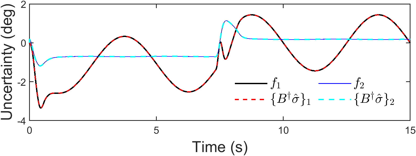
Figure 4: Actual and estimated uncertainties under UC-MPC. For $i=1,2$, the symbols $f_{j}$ and $\{B^{\dagger}\hat{\sigma}\}_{i}$ denotes the $i$th element of $f$ and $B^{\dagger}\hat{\sigma}$, respectively.

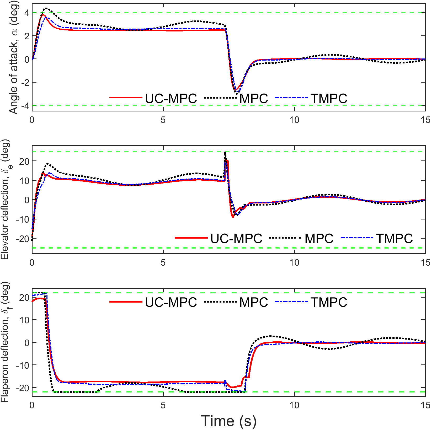
Figure 5: Trajectories of constrained states (top), and control inputs (middle and bottom) under MPC, TMPC, and UC-MPC. Green dash-dotted lines illustrate the constraints specified in 47.

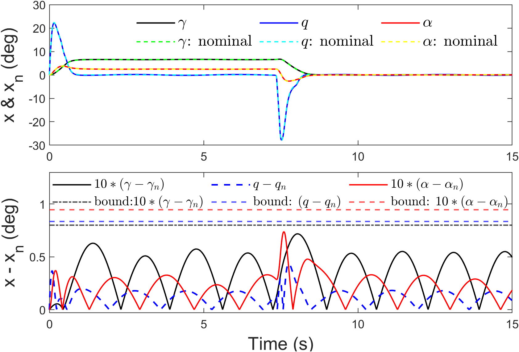
Figure 6: Trajectories of states of the uncertain system ($x(t)$) under UC-MPC and of the nominal system ($x_{\textup{n}}(t)$) and their differences. The actual-nominal state errors and bounds for $\gamma(t)$ and $\alpha$ are scaled by 10 for a clear illustration.

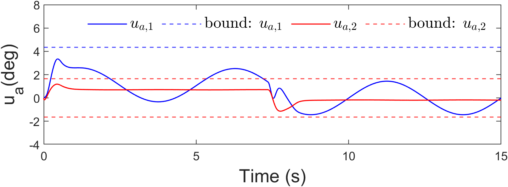
Figure 7: Adaptive control inputs and theoretical bounds

Regarding tracking performance, Figs. 2 and 3 show that UC-MPC yielded a better tracking performance compared with both MPC and TMPC, achieving a small error between the actual output $y(t)$ and the reference trajectory $r(t)$. This is because the adaptive control input $u_{a}(t)$ from UC-MPC approximately cancels the matched uncertainty $f(t,x(t))$, and, according to Fig. 4, the matched uncertainty estimation from UC-MPC was accurate. Due to the existence of the unmatched uncertainty $w(t)$, from the zoomed-in view in Fig. 3, we can see that the output trajectories from UC-MPC did not precisely follow the reference trajectories in steady-state, exhibiting an oscillation that has the same frequency as $w(t)$. In contrast, the output trajectories under MPC and TMPC were influenced by both the matched uncertainty and unmatched uncertainty, resulting in a larger tracking error.

Regarding constraints enforcement, Fig. 5 shows that both TMPC and UC-MPC successfully enforced all constraints due to the constraint tightening. In contrast, the output of MPC violated the state constraint as uncertainties were ignored during optimization without constraint tightening. It is also worth mentioning that TMPC enforced the constraints at the cost of larger steady-state tracking error, as shown in Fig. 3.

The trajectories of the actual state $x(t)$ and the nominal state $x_{\textup{n}}(t)$, as well as the error between them, and the derived individual bounds from ${\mathcal{L}_{1}}$AC are presented in Fig. 6. Under UC-MPC, it is evident that the actual states consistently remained in close proximity to the nominal states, exhibiting a difference smaller than the computed individual bound. Similarly, according to Fig. 7, the adaptive control inputs $u_{\textup{a}}(t)$ remained within the theoretical bounds calculated according to 41b.

In addition to the simulation above, we also conducted an experiment in the presence of only matched uncertainties, i.e., $w(t)=0$. Under such a scenario, as shown in Fig. 8, the proposed UC-MPC could successfully compensate for the uncertainty and achieve almost perfect tracking in steady state. Achieving such a high-accuracy tracking performance is not possible with existing robust or tube MPC methods, while the tracking performance of adaptive MPC approaches will also be limited in the presence of inaccurate parameter estimation.

Figure 8: Zoomed-in view of tracking performance on $\theta$ under MPC, TMPC and UC-MPC when $w(t)=0$

VII Conclusion

In this paper, we introduced an uncertainty compensation-based robust adaptive MPC framework, denoted as UC-MPC, for linear systems with both matched and unmatched uncertainties subject to both state and input constraints. Our approach leverages an adaptive controller to actively estimate and compensate for matched uncertainties, ensuring uniform performance bounds on the error between the states and inputs of the actual system and those of an uncertainty-free system. Then, the uniform performance bounds are used to tighten the constraints of the actual system, and an MPC problem is designed for the nominal system with the tightened constraints. Simulation results on a flight control problem demonstrate the efficacy of the proposed UC-MPC in achieving improved performance compared with existing methods while enforcing constraints.

Before presenting the proofs of the lemmas presented in this paper, we first introduce the following lemmas.

Lemma 5.

[16, Lemma 2] For a stable proper MIMO system $\mathcal{H}(s)$ with states $x(t)\in\mathbb{R}^{n}$, inputs $u(t)\in\mathbb{R}^{m}$ and outputs $y(t)\in\mathbb{R}^{p}$, under zero initial states, i.e., $x(0)=0$, we have $\left\lVert y\right\rVert_{\mathcal{L}_{\infty}^{[0,\tau]}}\leq\left\lVert\mathcal{H}(s)\right\rVert_{\mathcal{L}_{1}}\left\lVert u\right\rVert_{\mathcal{L}_{\infty}^{[0,\tau]}}$, for any $\tau\geq 0$. Furthermore, for any matrix $\mathrm{T}\in\mathbb{R}^{q\times p}$, we have $\left\lVert\mathrm{T}\mathcal{H}(s)\right\rVert_{\mathcal{L}_{\infty}}\leq\left\lVert\mathrm{T}\right\rVert_{\infty}\left\lVert\mathcal{H}(s)\right\rVert_{\mathcal{L}_{\infty}}$.

Lemma 6.

For the closed-loop reference system in 26 subject to Assumption 1 and the stability condition in 13a, we have

$$\left\lVert x_{\textup{r}}\right\rVert_{\mathcal{L}_{\infty}} <\rho_{r},$$ (49)

$$\left\lVert u_{\textup{r}}\right\rVert_{\mathcal{L}_{\infty}} <\rho_{ur},$$ (50)

where $\rho_{r}$ is introduced in 13a, and $\rho_{ur}$ is defined in 23f.

Proof.

For notation brevity, we define:

$$\eta(t)\triangleq f(t,x(t)),\quad\eta_{\textup{r}}(t)\triangleq f(t,x_{\textup{r}}(t)).$$ (51)

Let’s first rewrite the dynamics of the reference system in 26 in the Laplace domain:

$$x_{\textup{r}}(s)=\mathcal{G}_{xm}(s)\mathfrak{L}\left[f(t,x_{\textup{r}}(t))\right]+\mathcal{H}_{xm}(s)u_{\text{opt}}(s)$$

$$+\mathcal{H}_{xu}(s)w(s)+x_{\textup{in}}(s).$$ (52)

Considering 19, $A_{m}$ is Hurwitz and $\mathcal{X}_{0}$ is compact, we have $\left\lVert x_{\textup{in}}\right\rVert_{\mathcal{L}_{\infty}}\leq\rho_{\textup{in}}$ according to Lemma 5. As a result, according to Lemma 5 and because $\left\lVert w\right\rVert_{\mathcal{L}_{\infty}}\leq b_{w}$, for any $\xi>0$, we have

$$\left\lVert x_{\textup{r}}\right\rVert_{\mathcal{L}_{\infty}^{[0,\xi]}}\! \leq\left\lVert\mathcal{G}_{xm}(s)\right\rVert_{\mathcal{L}_{1}}\!\left\lVert\eta_{\textup{r}}\right\rVert_{\mathcal{L}_{\infty}^{[0,\xi]}}\!+\!\left\lVert\mathcal{H}_{xm}(s)\right\rVert_{\mathcal{L}_{1}}\left\lVert u_{\text{opt}}\right\rVert_{\mathcal{L}_{\infty}}$$

$$+\!\left\lVert\mathcal{H}_{xu}(s)\right\rVert_{\mathcal{L}_{1}}\!b_{w}\!+\!\left\lVert x_{\textup{in}}\right\rVert_{\mathcal{L}_{\infty}},$$ (53)

where $\eta_{\textup{r}}(t)$ is defined in 51. Assume by contradiction that 49 is not true. Since $x_{\textup{r}}(t)$ is continuous and $\left\lVert x_{\textup{r}}(0)\right\rVert_{\infty}<\rho_{r}$, there exists a $\tau\!>\!0$ such that

$$\left\lVert x_{\textup{r}}(t)\right\rVert_{\infty}<\rho_{r},\ \forall t\in[0,\tau),\ \textup{and}\ \left\lVert x_{\textup{r}}(\tau)\right\rVert_{\infty}=\rho_{r},$$ (54)

which implies $x_{\textup{r}}(t)\in\Omega(\rho_{r})$ for any $t$ in $[0,\tau]$. With 4b from Assumption 1, it follows that

$$\left\lVert\eta_{\textup{r}}\right\rVert_{\mathcal{L}_{\infty}^{[0,\tau]}}\leq b_{f,\Omega(\rho_{r})}.$$ (55)

By plugging the inequality above into Proof., we have

$$\rho_{r} \leq\left\lVert\mathcal{G}_{xm}(s)\right\rVert_{\mathcal{L}_{1}}b_{f,\Omega(\rho_{r})}+\left\lVert\mathcal{H}_{xm}(s)\right\rVert_{\mathcal{L}_{1}}\left\lVert u_{\text{opt}}\right\rVert_{\mathcal{L}_{\infty}}$$

$$+\left\lVert\mathcal{H}_{xu}(s)\right\rVert_{\mathcal{L}_{1}}b_{w}+\rho_{\textup{in}},$$ (56)

which contradicts the condition 13a. Therefore, 49 is true. Equation 50 immediately follows from 49 and 26. ∎

Lemma 7.

Given the uncertain system 8 subject to Assumption 1, the state predictor 20 and the adaptive law 21, if

$$\left\lVert x\right\rVert_{\mathcal{L}_{\infty}^{[0,\tau]}}\leq\rho,\quad\left\lVert u_{\textup{a}}\right\rVert_{\mathcal{L}_{\infty}^{[0,\tau]}}\leq\rho_{u_{\textup{a}}},$$ (57)

with $\rho$ and $\rho_{u_{\textup{a}}}$ defined in 23h and 14, respectively, then

$$\left\lVert\tilde{x}\right\rVert_{\mathcal{L}_{\infty}^{[0,\tau]}}\leq\gamma_{0}(T).$$ (58)

Proof.

Based on 57, we have $x(t)\in\Omega(\rho)$ for any $t$ in $[0,\tau]$. Due to 4b from Assumption 1, it follows that

$$\left\lVert f(t,x(t))\right\rVert_{\infty}=\left\lVert\eta(t)\right\rVert_{\infty}\leq b_{f,\Omega(\rho)},\quad\forall t\in[0,\tau].$$ (59)

From 8 and 20, the prediction error dynamics are given by

$$\dot{\tilde{x}}(t) =A_{e}\tilde{x}(t)+\hat{\sigma}(t)-Bf(t,x(t))-B_{u}w(t).$$ (60)

For any $0\leq t<T$ and $i\in\mathbb{Z}_{0}$, due to 60, we have

$$\tilde{x}(iT+t) =~{}e^{A_{e}t}\tilde{x}(iT)+\int_{iT}^{iT+t}e^{A_{e}(iT+t-\xi)}\hat{\sigma}(iT)d\xi$$

$$-\int_{iT}^{iT+t}e^{A_{e}(iT+t-\xi)}\left(B\eta(\xi)+B_{u}w(\xi)\right)d\xi$$

$$=~{}e^{A_{e}t}\tilde{x}(iT)+\int_{0}^{t}e^{A_{e}(t-\xi)}\hat{\sigma}(iT)d\xi$$

$$-\int_{0}^{t}e^{A_{e}(t-\xi)}\left(B\eta(iT+\xi)+B_{u}w(iT+\xi)\right)d\xi.$$ (61)

According to the adaptive law 21, the preceding equality implies

$$\tilde{x}((i+1)T)\!=$$

$$-\!\int_{0}^{T}\!e^{A_{e}(T-\xi)}\left(B\eta(iT+\xi)+B_{u}w(iT+\xi)\right)d\xi.$$ (62)

Therefore, considering 59, for any $i\in\mathbb{Z}_{0}$ with $(i+1)T\leq\tau$, we have

$$\left\lVert\tilde{x}((i+1)T)\right\rVert_{\infty} \leq\bar{\alpha}_{0}(T)b_{f,\Omega(\rho)}+\bar{\alpha}_{1}(T)b_{w},$$ (63)

where $\bar{\alpha}_{0}(T)$ and $\bar{\alpha}_{1}(T)$ are defined in 23a and 23b, respectively. Since $\tilde{x}(0)=0$,

$$\left\lVert\tilde{x}(iT)\right\rVert_{\infty}\leq\bar{\alpha}_{0}(T)b_{f,\Omega(\rho)}+\bar{\alpha}_{1}(T)b_{w}\leq\gamma_{0}(T),$$

$$\;\forall iT\leq\tau,i\in\mathbb{Z}_{0}.$$ (64)

Now we consider any $t\in(0,T]$ such that $iT+t\leq\tau$ with $i\in\mathbb{Z}_{0}$. From 61 and the adaptive law 21, we have

$$\left\lVert\tilde{x}(iT+t)\right\rVert_{\infty}\leq\left\lVert e^{A_{e}t}\right\rVert_{\infty}\left\lVert\tilde{x}(iT)\right\rVert_{\infty}$$

$$+\int_{0}^{t}\left\lVert e^{A_{e}(t-\xi)}\Phi^{-1}(T)e^{A_{e}T}\right\rVert_{\infty}\left\lVert\tilde{x}(iT)\right\rVert_{\infty}d\xi$$

$$+\int_{0}^{t}\left\lVert e^{A_{e}(t-\xi)}B\right\rVert_{\infty}\left\lVert\eta(iT+\xi)\right\rVert_{\infty}d\xi$$

$$+\int_{0}^{t}\left\lVert e^{A_{e}(t-\xi)}B_{u}\right\rVert_{\infty}\left\lVert w(iT+\xi)\right\rVert_{\infty}d\xi$$

$$\leq\left(\bar{\alpha}_{2}(T)+\bar{\alpha}_{3}(T)+1\right)(\bar{\alpha}_{0}(T)b_{f,\Omega(\rho)}+\bar{\alpha}_{1}(T)b_{w})$$

$$=\gamma_{0}(T),$$ (65)

where $\bar{\alpha}_{i}(T)$ ($i=0,1,2,3$) are defined in 23a, 23b and 23c, and the last inequality is partially due to the fact that $\int_{0}^{t}\left\lVert e^{A_{e}(t-\xi)}B\right\rVert_{\infty}d\xi\leq\int_{0}^{T}\left\lVert e^{A_{e}(T-\xi)}B\right\rVert_{\infty}\!d\xi\!=\!\bar{\alpha}_{0}(T)$ and $\int_{0}^{t}\left\lVert e^{A_{e}(t-\xi)}B_{u}\right\rVert_{\infty}d\xi\leq\int_{0}^{T}\left\lVert e^{A_{e}(T-\xi)}B_{u}\right\rVert_{\infty}\!d\xi\!=\!\bar{\alpha}_{1}(T)$. Equations Proof. and 65 imply 58. ∎

Appendix A Proofs

A-A Proof of Lemma 1

Proof.

27c and 27d are proved by contradiction. Assume that 27c or 27d do not hold. Since $\left\lVert x_{\textup{r}}(0)-x(0)\right\rVert_{\infty}=0<\gamma_{1}$, $\left\lVert u_{\textup{r}}(0)-u_{\textup{a}}(0)\right\rVert_{\infty}=0<\gamma_{2}$, and $x(t)$, $u_{\textup{a}}(t)$, $x_{\textup{r}}(t)$ and $u_{\textup{r}}(t)$ are all continuous, there must exist a time instant $\tau$ such that

$$\left\lVert x_{\textup{r}}(\tau)-x(\tau)\right\rVert_{\infty}=\gamma_{1}\textup{ or }\left\lVert u_{\textup{r}}(\tau)-u(\tau)\right\rVert_{\infty}=\gamma_{2},$$ (66)

and

$$\left\lVert x_{\textup{r}}(t)\!-\!x(t)\right\rVert_{\infty}\!<\!\gamma_{1},\ \left\lVert u_{\textup{r}}(t)\!-\!u(t)\right\rVert_{\infty}\!<\!\gamma_{2},\ \forall t\in[0,\tau).$$ (67)

It follows that at least one of the following equalities must hold:

$$\left\lVert x_{\textup{r}}-x\right\rVert_{\mathcal{L}_{\infty}^{[0,\tau]}}=\gamma_{1},\quad\left\lVert u_{\textup{r}}-u_{\textup{a}}\right\rVert_{\mathcal{L}_{\infty}^{[0,\tau]}}=\gamma_{2}.$$ (68)

According to Lemma 6, we have $\left\lVert x_{\textup{r}}\right\rVert_{\mathcal{L}_{\infty}}\leq\rho_{r}<\rho$ and according to 68, we have $\left\lVert x\right\rVert_{\mathcal{L}_{\infty}}\leq\rho_{r}+\gamma_{1}=\rho$. Further considering 4a that results from Assumption 1, we achieve

$$\left\lVert f(t,x_{\textup{r}}(t))\!-\!f(t,x(t))\right\rVert_{\infty}\!\leq\!L_{f,\Omega(\rho)}\!\left\lVert x_{\textup{r}}\!-\!x\right\rVert_{\mathcal{L}_{\infty}^{[0,\tau]}}\!,\ \forall t\!\in\![0,\tau].$$ (69)

The control laws in 22 and 26 indicate that

$$u_{\textup{r}}(s)-u_{\textup{a}}(s)=-{\mathcal{C}}(s)\mathfrak{L}\left[f(t,x_{\textup{r}})-B^{\dagger}\hat{\sigma}(t)\right]=$$

$${\mathcal{C}}(s)\mathfrak{L}\left[f(t,x)\!-\!f(t,x_{\textup{r}})\right]+{\mathcal{C}}(s)(B^{\dagger}\hat{\sigma}(s)\!-\!\mathfrak{L}\left[f(t,x)\right]).$$ (70)

From equation 60, we have

$$B^{\dagger}\hat{\sigma}(s)-\mathfrak{L}\left[f(t,x)\right])=B^{\dagger}(sI_{n}-A_{e})\tilde{x}(s).$$ (71)

Considering 8, 22 and 71, we have

$$x(s)\! =\mathcal{G}_{xm}(s)\mathfrak{L}\left[f(t,x)\right]\!+\!\mathcal{H}_{xm}(s)u_{\text{opt}}(s)\!+\!\mathcal{H}_{xu}(s)w(s)$$

$$+x_{\textup{in}}(s)-\mathcal{H}_{xm}(s){\mathcal{C}}(s)B^{\dagger}(sI_{n}-A_{e})\tilde{x}(s),$$ (72)

which, together with Proof., implies

$$x_{\textup{r}}(s)-x(s)=\mathcal{G}_{xm}(s)\mathfrak{L}\left[f(t,x_{\textup{r}})-f(t,x)\right]$$

$$+\mathcal{H}_{xm}(s){\mathcal{C}}(s)B^{\dagger}(sI_{n}-A_{e})\tilde{x}(s).$$ (73)

Therefore, due to 69 and Lemma 7, we have

$$\left\lVert x_{\textup{r}}-x\right\rVert_{\mathcal{L}_{\infty}^{[0,\tau]}} \leq\left\lVert\mathcal{G}_{xm}\right\rVert_{\mathcal{L}_{1}}L_{f,\Omega(\rho)}\left\lVert x_{\textup{r}}-x\right\rVert_{\mathcal{L}_{\infty}^{[0,\tau]}}$$ (74)

$$+\!\left\lVert\mathcal{H}_{xm}(s){\mathcal{C}}(s)B^{\dagger}(sI_{n}-A_{e})\right\rVert_{\mathcal{L}_{1}}\!\gamma_{0}(T).$$

The preceding equation, together with 13b, leads to

$$\left\lVert x_{\textup{r}}-x\right\rVert_{\mathcal{L}_{\infty}^{[0,\tau]}} \!\leq\!\frac{\left\lVert\mathcal{H}_{xm}(s){\mathcal{C}}(s)B^{\dagger}(sI_{n}\!-\!A_{e})\right\rVert_{\mathcal{L}_{1}}}{1-\left\lVert\mathcal{G}_{xm}\right\rVert_{\mathcal{L}_{1}}L_{f,\Omega(\rho)}}\gamma_{0}(T),$$ (75)

which, together with the sample time constraint 25, indicates that

$$\left\lVert x_{\textup{r}}-x\right\rVert_{\mathcal{L}_{\infty}^{[0,\tau]}}<\gamma_{1}.$$ (76)

On the other hand, it follows from 69, 70, 71 and 76 that

$$\left\lVert u_{\textup{r}}-u_{\textup{a}}\right\rVert_{\mathcal{L}_{\infty}^{[0,\tau]}}\leq\left\lVert{\mathcal{C}}(s)\right\rVert_{\mathcal{L}_{1}}L_{f,\Omega(\rho)}\left\lVert x_{\textup{r}}-x\right\rVert_{\mathcal{L}_{\infty}^{[0,\tau]}}$$

$$+\left\lVert{\mathcal{C}}(s)B^{\dagger}(sI_{n}-A_{e})\right\rVert_{\mathcal{L}_{1}}\left\lVert\tilde{x}\right\rVert_{\mathcal{L}_{\infty}^{[0,\tau]}}$$

$$<\left\lVert{\mathcal{C}}(s)\right\rVert_{\mathcal{L}_{1}}L_{f,\Omega(\rho)}\gamma_{1}+\left\lVert{\mathcal{C}}(s)B^{\dagger}(sI_{n}-A_{e})\right\rVert_{\mathcal{L}_{1}}\gamma_{0}(T).$$

Further considering the definition in 23g, we have

$$\left\lVert u_{\textup{r}}-u_{\textup{a}}\right\rVert_{\mathcal{L}_{\infty}^{[0,\tau]}}<\gamma_{2}.$$ (77)

Now, 76 and 77 contradict the 68, which shows that 27c and 27d holds. The bounds in 27a and 27b follow directly from 27c, 27d, 49 and 50 and the definitions of $\rho$ and $\rho_{u_{\textup{a}}}$ in 14 and 23h. The proof is complete. ∎

A-B Proof of Lemma 2

Proof.

Considering 9 and 26, we have

$$x_{\textup{r}}(s)-x_{\textup{n}}(s) =G_{xm}(s)\mathfrak{L}\left[f(t,x_{\textup{r}})\right]+\mathcal{H}_{xu}(s)w(s)$$

$$=G_{xm}(s)\mathfrak{L}\left[\eta_{\textup{r}}(t)\right]+\mathcal{H}_{xu}(s)w(s).$$ (78)

From Lemma 6, we have $x_{\textup{r}}(t)\in\Omega(\rho_{r})$ for any $t\geq 0$. Further because 4b that results from Assumption 1, it follows that $\left\lVert\eta_{\textup{r}}\right\rVert_{\mathcal{L}_{\infty}}\leq b_{f,\Omega(\rho_{r})}$, which, together with Section A-B, leads to 28. ∎

A-C Proof of Lemma 3

Proof.

Given any $\mathrm{T}_{x}^{i}$ satisfying 30 with an arbitrary $i\in\mathbb{Z}_{1}^{n}$, it follows that $\left\lVert\mathrm{T}_{x}^{i}\right\rVert_{\infty}=1$. As a result, using the transformation 29 and considering 34 and 36 and Lemma 5, the following inequalities hold

$$\left\lVert\mathcal{H}_{\check{x}m}^{i}(s)\right\rVert_{\mathcal{L}_{\infty}}\! \!\leq\!\left\lVert\mathrm{T}_{x}^{i}\right\rVert_{\infty}\!\left\lVert\mathcal{H}_{xm}(s)\right\rVert_{\mathcal{L}_{\infty}}\!\!=\!\left\lVert\mathcal{H}_{xm}(s)\right\rVert_{\mathcal{L}_{\infty}}\!,$$ (79a)

$$\left\lVert\mathcal{H}_{\check{x}u}^{i}(s)\right\rVert_{\mathcal{L}_{\infty}}\! \!\leq\!\left\lVert\mathrm{T}_{x}^{i}\right\rVert_{\infty}\!\left\lVert\mathcal{H}_{xu}(s)\right\rVert_{\mathcal{L}_{\infty}}\!=\!\left\lVert\mathcal{H}_{xu}(s)\right\rVert_{\mathcal{L}_{\infty}}\!,$$ (79b)

$$\left\lVert\mathcal{G}_{\check{x}m}^{i}(s)\right\rVert_{\mathcal{L}_{\infty}}\! \!\leq\!\left\lVert\mathrm{T}_{x}^{i}\right\rVert_{\infty}\!\left\lVert\mathcal{G}_{xm}(s)\right\rVert_{\mathcal{L}_{\infty}}\!=\!\left\lVert\mathcal{G}_{xm}(s)\right\rVert_{\mathcal{L}_{\infty}}\!,$$ (79c)

$$\check{\rho}_{\textup{in}}^{i} \!\leq\!\left\lVert\mathrm{T}_{x}^{i}\right\rVert_{\infty}\rho_{\textup{in}}\!=\!\rho_{\textup{in}}.$$ (79d)

The property of $x_{\textup{r}}(t)\in\mathcal{X}_{r}$ for any $t\geq 0$ from Lemma 6 and 29 together imply $\check{x}_{\textup{r}}(t)\in\check{\mathcal{X}}_{r}$ for any $t\geq 0$, where $\check{\mathcal{X}}_{r}$ is defined via 33. Considering 32 and 33, for any compact set $\mathcal{X}_{r}$, we have

$$b_{\check{f},\check{\mathcal{X}}_{r}}=b_{f,\mathcal{X}_{r}}.$$ (80)

Suppose that constants $\rho_{r}$ and $\left\lVert u_{\text{opt}}\right\rVert_{\mathcal{L}_{\infty}}$ satisfy 13a. According to 80 and 79, with $\check{\rho}_{r}^{i}=\rho_{r}$ and the same $\left\lVert u_{\text{opt}}\right\rVert_{\mathcal{L}_{\infty}}$, 37 is satisfied.

In addition, if 37 holds, through the application of Lemma 6 to the transformed reference system 31, we obtain $\left\lVert\check{x}_{\textup{r}}\right\rVert_{\mathcal{L}_{\infty}}\leq\check{\rho}_{r}^{i}$, which further implies that $\left\lvert\check{x}_{\textup{r},i}(t)\right\rvert\leq\check{\rho}_{r}^{i}$ for any $t\geq 0$. Since $\check{x}_{\textup{r},i}(t)=x_{\textup{r},i}(t)$ due to the constraint 30 on $\mathrm{T}_{x}^{i}$, we have 38. Equation 38 is equivalent to $x_{\textup{r}}(t)\in\mathcal{X}_{r}$ for any $t\geq 0$, with the re-definition of $\mathcal{X}_{r}$ in 40. Following the proof of Lemma 2, we are able to obtain $\left\|{\check{x}_{\textup{r}}-\check{x}_{\textup{n}}}\right\|_{{\mathcal{L}}{{}_{\infty}}}\leq\left\lVert\mathcal{G}_{\check{x}m}\right\rVert_{\mathcal{L}_{1}}b_{\check{f},\check{\mathcal{X}}_{r}}+\left\lVert\mathcal{H}_{\check{x}u}\right\rVert_{\mathcal{L}_{1}}b_{w}=\left\lVert\mathcal{G}_{\check{x}m}(s)\right\rVert_{\mathcal{L}_{1}}b_{f,\mathcal{X}_{r}}+\left\lVert\mathcal{H}_{\check{x}u}\right\rVert_{\mathcal{L}_{1}}b_{w}$, where the equality comes from 80. Further considering $\check{x}_{\textup{r},i}(t)=x_{\textup{r},i}(t)$ and $\check{x}_{\textup{n},i}(t)=x_{\textup{n},i}(t)$ due to the constraint 30 on $\mathrm{T}_{x}^{i}$, we finally have 39. ∎

A-D Proof of Lemma 4

Proof.

For each $i\in\mathbb{Z}_{1}^{n}$, Lemma 3 implies that $\left\lvert x_{\textup{r},i}(t)\right\rvert\leq\check{\rho}_{r}^{i}$ and $\left\lvert x_{\textup{r,i}}(t)-x_{\textup{n},i}(t)\right\rvert\leq\left\lVert\mathcal{G}_{\check{x}m}^{i}(s)\right\rVert_{\mathcal{L}_{1}}b_{f,\mathcal{X}_{r}}+\left\lVert\mathcal{H}^{i}_{\check{x}u}\right\rVert_{\mathcal{L}_{1}}b_{w}$ for all $t\geq 0$. From Lemma 1, it follows that $\left\lvert x_{\textup{r},i}(t)-x_{i}(t)\right\rvert\leq\gamma_{1}$ for any $t\geq 0$ and any $i\in\mathbb{Z}_{1}^{n}$. Thus, 41a is true. On the other hand, Lemma 1 indicates that $\left\lvert u_{\textup{r},j}(t)-u_{\textup{a},j}(t)\right\rvert\leq\gamma_{2}$ for any $t\geq 0$. Property 26 and the structure of ${\mathcal{C}}(s)$ in 12 lead to

$$u_{\textup{r},j}(s)=-{\mathcal{C}}_{j}(s)\mathfrak{L}\left[f_{j}(t,x_{\textup{r}}(t))\right],\quad\forall j\in\mathbb{Z}_{1}^{m}.$$ (81)

Therefore, given a set $\mathcal{X}_{r}$ such that $x_{\textup{r}}(t)\!\in\!\mathcal{X}_{r}$ for any $t\!\geq\!0$, from Assumptions 1 and 5, the following property holds

$$\left\lvert u_{\textup{r},j}(t)\right\rvert\leq\left\lVert{\mathcal{C}}_{j}(s)\right\rVert_{\mathcal{L}_{1}}b_{f_{j},\mathcal{X}_{r}},\quad\forall t\geq 0,\ \forall j\in\mathbb{Z}_{1}^{m}.$$ (82)

Thus, for any $j\in\mathbb{Z}_{1}^{m}$, we have 41b. Finally, since $u(t)-u_{\textup{n}}(t)=K_{x}(x(t)-x_{\textup{n}}(t))+u_{\textup{a}}(t)$, we achieve 41c. The proof is complete. ∎

References

• [1] E. F. Camacho and C. B. Alba, Model predictive control. Springer Science & Business Media, 2013.
• [2] J. B. Rawlings, D. Q. Mayne, and M. M. Diehl, Model Predictive Control: Theory, Computation, and Design, 2nd Ed. Nob Hill Publishing, 2020.
• [3] S. Yu, M. Reble, H. Chen, and F. Allgöwer, “Inherent robustness properties of quasi-infinite horizon nonlinear model predictive control,” Automatica, vol. 50, no. 9, pp. 2269–2280, 2014.
• [4] E. C. Kerrigan, Robust constraint satisfaction: Invariant sets and predictive control. PhD thesis, University of Cambridge, 2001.
• [5] W. Langson, I. Chryssochoos, S. Raković, and D. Q. Mayne, “Robust model predictive control using tubes,” Automatica, vol. 40, no. 1, pp. 125–133, 2004.
• [6] S. Rakovic, Robust control of constrained discrete time systems: Characterization and implementation. PhD thesis, University of London, 2005.
• [7] D. Q. Mayne, S. V. Raković, R. Findeisen, and F. Allgöwer, “Robust output feedback model predictive control of constrained linear systems,” Automatica, vol. 42, no. 7, pp. 1217–1222, 2006.
• [8] D. Q. Mayne, E. C. Kerrigan, E. Van Wyk, and P. Falugi, “Tube-based robust nonlinear model predictive control,” International Journal of Robust and Nonlinear Control, vol. 21, no. 11, pp. 1341–1353, 2011.
• [9] J. Köhler, R. Soloperto, M. A. Müller, and F. Allgöwer, “A computationally efficient robust model predictive control framework for uncertain nonlinear systems,” IEEE Transactions on Automatic Control, vol. 66, no. 2, pp. 794–801, 2020.
• [10] B. T. Lopez, J.-J. E. Slotine, and J. P. How, “Dynamic tube MPC for nonlinear systems,” in Proceedings of American Control Conference, pp. 1655–1662, 2019.
• [11] S. V. Rakovic and W. S. Levine, “Handbook of model predictive control,” 2018.
• [12] V. Adetola and M. Guay, “Robust adaptive mpc for constrained uncertain nonlinear systems,” International Journal of Adaptive Control and Signal Processing, vol. 25, no. 2, pp. 155–167, 2011.
• [13] A. Sasfi, M. N. Zeilinger, and J. Köhler, “Robust adaptive mpc using control contraction metrics,” Automatica, vol. 155, p. 111169, 2023.
• [14] M. Lorenzen, F. Allgöwer, and M. Cannon, “Adaptive model predictive control with robust constraint satisfaction,” IFAC-PapersOnLine, vol. 50, no. 1, pp. 3313–3318, 2017.
• [15] K. Zhang and Y. Shi, “Adaptive model predictive control for a class of constrained linear systems with parametric uncertainties,” Automatica, vol. 117, p. 108974, 2020.
• [16] P. Zhao, I. Kolmanovsky, and N. Hovakimyan, “Integrated adaptive control and reference governors for constrained systems with state-dependent uncertainties,” IEEE Transactions on Automatic Control, conditionally accepted, 2022. arXiv preprint arXiv:2208.02985.
• [17] N. Hovakimyan and C. Cao, $\mathcal{L}_{1}$ Adaptive Control Theory: Guaranteed Robustness with Fast Adaptation. Philadelphia, PA: Society for Industrial and Applied Mathematics, 2010.
• [18] K. Pereida, L. Brunke, and A. P. Schoellig, “Robust adaptive model predictive control for guaranteed fast and accurate stabilization in the presence of model errors,” International Journal of Robust and Nonlinear Control, vol. 31, no. 18, pp. 8750–8784, 2021.
• [19] L. Magni and R. Scattolini, “Stabilizing model predictive control of nonlinear continuous time systems,” Annual Reviews in Control, vol. 28, no. 1, pp. 1–11, 2004.
• [20] J. B. Rawlings, D. Q. Mayne, and M. Diehl, Model Predictive Control: Theory, Computation, and Design, vol. 2. Madison, WI: Nob Hill Publishing, 2017.
• [21] K. M. Sobel and E. Y. Shapiro, “A design methodology for pitch pointing flight control systems,” Journal of Guidance, Control, and Dynamics, vol. 8, no. 2, pp. 181–187, 1985.
• [22] D. Q. Mayne, M. M. Seron, and S. Raković, “Robust model predictive control of constrained linear systems with bounded disturbances,” Automatica, vol. 41, no. 2, pp. 219–224, 2005.