Unique continuation on planar graphs

Abstract.

We show that a discrete harmonic function which is bounded on a large portion of a periodic planar graph is constant. A key ingredient is a new unique continuation result for the weighted graph Laplacian. The proof relies on the structure of level sets of discrete harmonic functions, using arguments as in Bou-Rabee–Cooperman–Dario (2023) which exploit the fact that, on a planar graph, the sub- and super-level sets cannot cross over each other. In the special case of the square lattice this yields a new, geometric proof of the Liouville theorem of Buhovsky–Logunov–Malinnikova–Sodin (2017).

1. Introduction

A periodic planar graph $\mathcal{G}=(\mathcal{V},\mathcal{E})$ is a graph for which there exists an embedding into the plane $\operatorname{\mathbb{R}}^{2}$ which is invariant under translation by a two-dimensional-lattice $\mathcal{L}$. We fix such an embedding and consider the weighted graph Laplacian on $\mathcal{G}$,

$$\Delta f(u)=\sum_{w\sim u}\mathbf{a}(u,w)(f(u)-f(w))\,,$$

where the sum is over the vertices $w\in\mathcal{V}$ adjacent to $u$ and the conductance, $\mathbf{a}$, is a strictly positive function on the set of undirected edges $\mathcal{E}$. Designate a vertex closest to zero as the origin and let $B_{n}$ denote the graph-metric ball of radius $n$ centered at the origin. We write $\mathcal{F}:=\mathcal{G}/2\mathcal{L}$ to denote a (finite) quotient of the graph which, together with $\mathcal{L}$, contains all of the information needed to reconstruct $\mathcal{G}$. Abusing notation, we identify the vertex set $\mathcal{V}$ of $\mathcal{G}$ with its image in $\operatorname{\mathbb{R}}^{2}$ under the embedding.

Figure 1. Some periodic planar graphs.

Recall that any bounded harmonic function on $\mathcal{G}$ is constant. Our main result is the following improvement of this Liouville theorem.

Theorem 1.1.

Suppose that the conductances $\mathbf{a}$ are invariant under translation by $\mathcal{L}$. Then there is some $\varepsilon=\varepsilon(\mathbf{a})>0$ such that, if $\Delta f=0$ on $\mathcal{G}$ and

$$\lim_{n\to\infty}\frac{|\{|f|\leq 1\}\cap B_{n}|}{|B_{n}|}\geq 1-\varepsilon\,,$$

then $f$ is constant.

In the special case of $\operatorname{\mathbb{Z}}^{2}$ with unit conductance, Buhovsky–Logunov–Malinnikova–Sodin in [BLMS22] established Theorem 1.1 via a delicate argument involving the polynomial structure of discrete harmonic functions on $\operatorname{\mathbb{Z}}^{2}$. They proved two competing statements. First they showed, using the three-ball inequality, that a non-constant discrete harmonic function which is bounded on most of $\operatorname{\mathbb{Z}}^{2}$ must grow at least exponentially. This result is quite general and, as we indicate in the appendix, also holds for periodic graphs. Second, using the square lattice structure, they proved an exponential upper bound for the growth of such a function, with an exponent which tends to zero as $\varepsilon\to 0$. One of their key observations is that a discrete harmonic function on $\operatorname{\mathbb{Z}}^{2}$, which vanishes on two parallel diagonals, is equal (up to a sign) to a polynomial on subsequent diagonals. Unfortunately, this polynomial structure is no longer present on general planar graphs, or even on $\operatorname{\mathbb{Z}}^{2}$ when the conductances are not constant.

Our main contribution is a completely new proof of this exponential upper bound. This may also be thought of as a unique continuation result. The argument is based on a topological property of the level sets of planar discrete harmonic functions and is therefore robust to changes in the underlying graph. Similar topological arguments were previously used by Dario and the first two authors in a study of harmonic functions on the supercritical percolation cluster [BRCD23].

Some basic features of non-crossing level sets in the plane have been used previously, e.g., in Serrin’s proof of the Harnack inequality [Ser56]. We take a more quantitative approach and study the structure of the intersection points between sub- and super-level sets of zero. On the one hand, planarity forces these two sets to interleave and this ensures the existence of many distinct connected components of each set. On the other, each component intersects at least one vertex on the boundary of the domain, so there cannot be too many.

Theorem 1.2.

Suppose the conductances are uniformly bounded via $0<\lambda<\mathbf{a}<\Lambda<\infty$. Then there exist positive constants $\varepsilon_{0}(\mathcal{F},\Lambda/\lambda)$, $n_{0}(\mathcal{F})$, and $A(\mathcal{F},\Lambda/\lambda)$ such that for all $n\geq n_{0}$ and $\varepsilon<\varepsilon_{0}$, if $\Delta f=0$ on $B_{2n}$ and $|\{x\in B_{2n}\mid|f(x)|>1\}|\leq\varepsilon|B_{2n}|$, then $\max_{B_{n}}|f|\leq e^{(A\sqrt{\varepsilon})n}$.

Following the arguments in [BLMS22], the exponential lower bound, Theorem A.1, together with the exponential upper bound, Theorem 1.2, establishes Theorem 1.1.

The same argument to prove Theorem 1.2 can be used to provide a short proof of Theorem 1.1 (with no assumptions on $\mathbf{a}$ other than positivity) when the discrete harmonic function is not just bounded but also vanishes on a large portion of the graph.

Theorem 1.3.

There exist positive constants $\varepsilon_{0}(\mathcal{F})$ and $n_{0}(\mathcal{F})$ such that if $\Delta f=0$ on $B_{2n}$ for $n\geq n_{0}$ and $|\{x\in B_{2n}\mid|f(x)|\neq 0\}|\leq\varepsilon|B_{2n}|$, for $\varepsilon<\varepsilon_{0}$, then $f\equiv 0$ on $B_{n}$.

Our theorems require the discrete two-dimensional structure as encapsulated in Lemma 2.1 below. As explained in [BLMS22, Remark 1.3], there counterexamples on $\operatorname{\mathbb{Z}}^{d}$ for $d\geq 3$ and on $\operatorname{\mathbb{R}}^{2}$. For instance, the function $(x,y,z)\to c^{z}(-1)^{x}1_{\{x=y\}}$ for $c$ satisfying $c+c^{-1}=6$ is harmonic on $\operatorname{\mathbb{Z}}^{3}$. Planarity is also essential — as indicated in Section 5, there is a family of non-planar conductances on $\operatorname{\mathbb{Z}}^{2}$ for which Theorem 1.3 fails.

An important application of unique continuation results of this form is Anderson localization. Ding–Smart [DS20] used ideas from [BLMS22] as input into the program of Bourgain–Kenig [BK05] to prove localization near the edge for the Anderson–Bernoulli model on $\operatorname{\mathbb{Z}}^{2}$. This result was generalized to $\operatorname{\mathbb{Z}}^{3}$ by Li–Zhang [LZ22], where, as part of their argument, they proved a version of Theorem 1.2 on the triangular lattice using ideas from [BLMS22].

Throughout $c,C$ denote positive constants that may differ in each instance. Dependence is indicated by, e.g., $C(d)$.

Acknowledgments

Thank you to Scott Armstrong, Paul Dario, Lionel Levine, and Charles Smart for useful discussions and suggestions. A.B. was partially supported by NSF grant DMS-2202940 and a Stevanovich fellowship. W.C. was partially supported by NSF grant DMS-2303355. S.G. was partially supported by NSF grants DMS-1855688, DMS-1945172, and a Sloan Fellowship.

2. A topological lemma

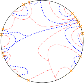
Figure 2. Sets satisfying the properties of Lemma 2.1. The cycle $\gamma$ is drawn as a black circle, the set $Z$ as dark orange crosses, and sets $P$ and $M$ as red dotted and blue dashed lines respectively.

We give a geometric constraint on the level sets of a discrete harmonic function $f$ on a planar graph. This is the key topological observation underlying our arguments. One may think of the set $Z$ as the zero set of $f$, the set $P$ as the zero superlevel set (pluses), and the set $M$ as the zero sublevel set (minuses). Roughly, the conclusion is that $f$ cannot have too many zeros on a circle without being identically zero in the half ball.

Lemma 2.1.

Let $\gamma:=\{v_{0},v_{1},\dots,v_{k}=v_{0}\}$ be a cycle in $\mathcal{G}$ and let sets $Z,P,M\subseteq\mathcal{V}$ be disjoint and satisfy the following properties.

1. $Z\subseteq\gamma$.

2. $P$ and $M$ are contained in the union of $\gamma$ and the finite component of $\mathcal{G}\setminus\gamma$.

3. For every $z\in Z$, there is a path $\beta:=\{z=w_{0},w_{1},\dots,w_{\ell}\}$ along a face of $\mathcal{G}$ adjacent to $z$, such that $\beta\cap(P\cup M)=\emptyset$ and $w_{\ell}$ is adjacent to vertices $p(z)\in P$ and $m(z)\in M$. If there are multiple such vertices, we choose $p(z)$ and $m(z)$ arbitrarily.

4. Every connected component of the induced subgraph $\mathcal{G}[P]$ (respectively of $\mathcal{G}[M]$) intersects $\gamma\setminus Z$.

Then, for a constant $\alpha_{\mathcal{F}}\in(0,1)$ depending only on the maximum degree in the graph $\mathcal{G}$, we have $|Z|\leq\alpha_{\mathcal{F}}|\gamma|$.

Proof.

For each $v_{i}\in Z$, we define $\operatorname{\mbox{prev}}_{P}(v_{i})\in\gamma\setminus Z$ (resp. $\operatorname{\mbox{prev}}_{M}(v_{i})$) to be $v_{i-j\pmod{k}}$, where $j$ is smallest in $\{1,\dots,k\}$ such that $v_{i-j\pmod{k}}$ lies in the connected component of $p(v_{i})$ in $\mathcal{G}[P]$ (resp. $m(v_{i})$ in $\mathcal{G}[M]$).

Let $Z=\{v_{j_{1}},v_{j_{2}},\dots,v_{j_{|Z|}}\}$, where $0\leq j_{1}<j_{2}<\cdots<j_{|Z|}<k$ and choose a maximal subset $Z^{\prime}=\{v_{i_{1}},v_{i_{2}},\dots,v_{i_{|Z|}}\}$ so that $p(z)\neq p(\tilde{z})$ and $m(z)\neq m(\tilde{z})$ for $z\neq\tilde{z}\in Z^{\prime}$. Note that by (3), we have that

(1) $$\frac{|Z^{\prime}|}{|Z|}\geq(2(\mbox{max degree in $\mathcal{G}$}))^{-1}\,.$$

We trace out the cycle $\gamma$ and argue, using planarity, that each time we encounter a vertex in $Z^{\prime}$, there must be a new vertex in $\gamma\setminus Z$. To that end, for each $j=0,\dots,|Z^{\prime}|$, we iteratively build sets $S_{j}\subseteq\gamma\setminus Z$ as follows. Start with $S_{0}:=\emptyset$. Given $j\geq 0$, consider three cases.

1. If $\operatorname{\mbox{prev}}_{P}(v_{i_{j}})\not\in S_{j}$ then set $S_{j+1}:=S_{j}\cup\{\operatorname{\mbox{prev}}_{P}(v_{i_{j}})\}$.

2. Otherwise, let $k<j$ be the smallest index such that $\operatorname{\mbox{prev}}_{P}(v_{i_{k}})=\operatorname{\mbox{prev}}_{P}(v_{i_{j}})$. If $k=j-1$, then set $S_{j+1}:=S_{j}$.

3. Otherwise, we set $S_{j+1}:=S_{j}\cup\{\operatorname{\mbox{prev}}_{M}(v_{i_{j-1}})\}$.

We claim that in each step we are only adding vertices which are not already in the set. We need only argue that in the third case, $\operatorname{\mbox{prev}}_{M}(v_{i_{j-1}})\not\in S_{j}$. However, observe that a vertex in $M$ is in $S_{j}$ only if it is enclosed by a loop with vertices $v_{i_{j}}$ and $v_{i_{k}}$ – see Figure 3 – and only one such vertex which is enclosed by the loop is added. Thus, by the Jordan curve theorem, the vertices in $M$ which are added must be disjoint.

Hence, by construction and (1), we have

$$|\gamma\setminus Z|\geq|S_{|Z^{\prime}|}|\geq\frac{1}{2}|Z^{\prime}|\geq(4(\mbox{max degree in $\mathcal{G}$}))^{-1}|Z|\,,$$

which concludes the proof. ∎

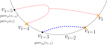
Figure 3. Case 3 in the proof of Lemma 2.1. Although the loop enclosing $\operatorname{\mbox{prev}}_{M}(v_{i-1})$ could touch $\gamma$ in multiple places this does not affect the proof. Note that the loop ensures that for all $j>i$ we have $\operatorname{\mbox{prev}}_{M}(v_{j})\neq v_{j^{\prime}}$ for each $j^{\prime}\in[i-4,i]$. The same color scheme as Figure 2 is used.

3. Many zeros implies identically zero

Let $\mathcal{G}^{*}$ be the dual graph of $\mathcal{G}$ whose vertices are the faces of $\mathcal{G}$ and whose edges correspond to adjacent faces of $\mathcal{G}$. Denote by $\partial B_{m}$ the set of faces in $\mathcal{G}^{*}$ which are adjacent to both $B_{m}$ and its complement.

We prove Theorem 1.3 in steps. In the first two steps, we reduce to the case where $\mathcal{G}^{*}$ is a graph (not a multigraph) and there are few nonzeros on the boundary of $B_{n}$. The third step is an argument by contradiction: if there were a nonzero vertex in $B_{n/2}$, then by Lemma 2.1 this would force many nonzeros on the boundary of $B_{n}$.

Step 1: Reduction to case when $\mathcal{G}^{*}$ is a graph.
First, we assume without loss of generality that $\mathcal{G}$ is 2-edge connected, because any harmonic function is constant on finite 2-edge connected components of $\mathcal{G}$.

Next, if $\mathcal{G}^{*}$ had multiple edges, then there would exist a finite connected component $K$ of $\mathcal{G}$ which is 3-edge connected and for which there are only two edges, $e_{1}$ and $e_{2}$, which connect $K$ to $\mathcal{G}\setminus K$. Let $\mathcal{G}^{\prime}$ be the graph $\mathcal{G}$, with $K$ replaced by a single edge connecting the endpoints of $e_{1}$ and $e_{2}$ in $\mathcal{G}\setminus K$. The weight of this new edge is given by the effective conductance of $K$ between the endpoints. Then any harmonic function on $\mathcal{G}$ is also harmonic when restricted to $\mathcal{G}^{\prime}$. Furthermore, since $\mathcal{G}$ is periodic, we can repeat this process for each finite 3-edge connected component of $\mathcal{G}$ and only remove a constant fraction of vertices from $\mathcal{G}$. Modifying the $\varepsilon_{0}$ in Theorem 1.3 appropriately according to this fraction, we see that proving the theorem for $\mathcal{G}^{\prime}$ implies the result for $\mathcal{G}$, and therefore we assume that $\mathcal{G}^{*}$ is a graph without loss of generality.

Step 2: Reduction to few non-zeros on the boundary.
By the pigeonhole principle and the assumption that $f=0$ on a $(1-\varepsilon)$ portion of $B_{2n}$, we may assume that there is some $\partial B_{m}$ for $m\in[1.5n,2n]$ such the number of vertices for which $f(v)\neq 0$ and which are adjacent to a face in $\partial B_{m}$ is at most $C\varepsilon n$.

Step 3: Bounding the number of zeros.
Let $m\in[1.5n,2n]$ be given by Step 2. Assume for contradiction that there is some $x_{0}\in B_{n}$ with $f(x_{0})\neq 0$. Let $N$ be the set of faces of $\mathcal{G}[B_{m}]$ which are adjacent to at least one vertex where $f$ is nonzero. Then the maximal connected component $K\subseteq N$ in $\mathcal{G}^{*}$ which contains every face adjacent to $x_{0}$ also contains, by the maximum principle, a face in $\partial B_{m}$. Let $\gamma:=\{v_{0},v_{1},\dots,v_{k}=v_{0}\}$ be a cycle in $\mathcal{G}$ around the boundary of $K\cup\{\text{vertices in finite connected components of $\mathcal{G}^{*}\setminus K$}\}$.

Let $D$ be the unique finite connected component of $\mathcal{G}\setminus\gamma$. First, we note that $D$ contains $x_{0}\in B_{n}$ and a vertex adjacent to $\partial B_{m}$, so it has diameter at least $n/2$ and therefore its boundary, $\gamma$, has length at least $n/2$. Our goal is to find suitable sets $Z,P,M$ to apply Lemma 2.1. Let $Z:=\gamma\setminus\{\mbox{vertices adjacent to $\partial B_{m}$}\}$ and let $P:=\{x\in\gamma\cup D\mid f(x)>0\}$ and $M:=\{x\in\gamma\cup D\mid f(x)<0\}$.

By maximality, $f(z)=0$ for every vertex $z\in Z$. It is clear that $Z,P,M$ are disjoint. Furthermore, the first two hypotheses of Lemma 2.1 are clearly satisfied. The fourth hypothesis of Lemma 2.1 is satisfied by the maximum principle. It remains to check the third hypothesis: fix any $z\in Z$. Since $z$ is adjacent to a face $F\in K$, there is some vertex $w$ adjacent to $F$ on which $f(w)\neq 0$. Choose $w$ to be the vertex closest to $z$ with this property, and let $\beta=\{z=w_{0},w_{1},\dots,w_{\ell}\}$ be a shortest path such that $w_{\ell}$ is adjacent to $w$. By minimality of $\beta$, we have $f(w_{\ell})=0$ and therefore $w_{\ell}$ is also adjacent to some vertex $y$ with $\operatorname{\mathop{\bf sgn}}f(y)=-\operatorname{\mathop{\bf sgn}}f(w)$. Then we set $p(z)$ to be the vertex in $\{w,y\}$ on which $f$ is positive, and $m(z)$ to be the other vertex in $\{w,y\}$. Since $f$ vanishes on $\beta$, we see that the third hypothesis of Lemma 2.1 is satisfied.

Applying Lemma 2.1, we conclude that $|Z|\leq\alpha_{\mathcal{F}}|\gamma|$. Hence, at least $(1-\alpha_{\mathcal{F}})$ vertices in $\gamma$ are adjacent to a face in $\partial B_{m}$. Each of these faces must be adjacent to a vertex for which $f$ is nonzero. However, since $|\gamma|\geq n/2$, this contradicts Step 2 for $\varepsilon_{0}$ sufficiently small, completing the proof.∎

Remark 3.1.

The argument shows that the density hypothesis in Theorem 1.3 may be replaced, as in Step 2, by a bound on the number of non-zero vertices adjacent to $\partial B_{2n}$. In particular, this shows that if there are infinitely many contours surrounding the origin for which the harmonic function has a high density of zeros, then the function must be zero identically.

4. Exponential upper bound

For the proof of Theorem 1.2, we have the additional hypothesis of uniformly ellipticity, $0<\lambda<\mathbf{a}<\Lambda$. This allows us to exploit the following observation: if $f(x)$ is small and there is a neighbor $y\sim x$ for which $f(y)$ has large magnitude, then there is a different neighbor $z\sim x$ with large magnitude of the opposite sign. Equipped with this observation we argue along similar lines as the proof of Theorem 1.3.

Step 1: An exponential bound.
In this step we prove that there exists $\varepsilon_{1}\in(0,1)$ such that if $\varepsilon\leq\varepsilon_{1}$

(2) $$\max_{B_{n}}|f|\leq C\alpha^{n}\,,$$

for constant exponent $\alpha$ depending only on $\mathcal{F}$ and the ellipticity ratio $\Theta:=\Lambda/\lambda$.

By the pigeonhole principle, for each $\delta\in(0,1)$, there is a sufficiently large $K(\delta)$ and an integer $A\in[1,K^{n}]$ for which $|\{v\in\mathcal{G}[B_{2n}]:|A|<|f(v)|<2\Theta\mbox{(max degree in $\mathcal{G}$)}A\}|<\delta n$. We may then repeat the proof of Theorem 1.3, treating $\{v\in\mathcal{G}[B_{2n}]\mid|f(v)|<|A|\}$ as the zero set. The only difference is that there is a $\delta$-fraction of “zeros” which do not satisfy condition (3) of Lemma 2.1, but since $\delta$ can be made arbitrarily small, we may discard those points from $Z$ before applying Lemma 2.1 and we have (2).

Step 2: Improve the exponent by covering.
Following the argument at the end of the proof of [BLMS22, Theorem A’], we upgrade the exponential bound from Step 1 to a bound involving $\varepsilon$. Let $\delta=C^{-1}\varepsilon_{1}^{-1/2}\varepsilon^{1/2}$ and cover $B_{n}$ by $\delta^{2}$ balls of radius $\delta n$ contained in $B_{2n}$, decreasing $\varepsilon_{0}$ if necessary. Observe that for each such ball $B_{\delta n}(z_{i})$, we have $|v\in B_{\delta n}(z_{i})\mid|f(v)|>1|<C\varepsilon\delta^{-2}|B_{\delta n}|=\varepsilon_{1}|B_{\delta n}|$ and hence, by applying Step 1 to each such ball, we have $\max_{B_{n}}|f|\leq\alpha^{(C^{-1}\varepsilon_{1}^{-1/2})\varepsilon^{1/2}n}$ which completes the proof. ∎

5. A non-planar counterexample on the square lattice

We present a collection of periodic conductances with crossing edges on $\operatorname{\mathbb{Z}}^{2}$ for which Theorem 1.3 fails. For each vertex $x$ such that $x_{1}+x_{2}$ is even, assign (undirected) conductances as follows

$$\mathbf{a}(x,x-e_{2})\,,\,\mathbf{a}(x,x-e_{1}):=A_{1}\qquad\mathbf{a}(x,x+e_{2})\,,\,\mathbf{a}(x,x+e_{1}):=A_{2}$$

$$\mathbf{a}(x,x+(2e_{1},2e_{2}))\,,\,\mathbf{a}(x,x-(2e_{1},2e_{2})):=A_{3}\qquad\mathbf{a}(x,x+(e_{1},e_{2}))\,,\,\mathbf{a}(x,x-(e_{1},e_{2})):=A_{4}\,,$$

see Figure 4. Denote this graph by $(\operatorname{\mathbb{Z}}^{2},\mathcal{E}(A_{1},A_{2},A_{3},A_{4}))$.

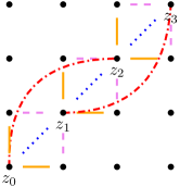
Figure 4. Conductances $A_{1},A_{2},A_{3},A_{4}$ are dashed violet lines, orange solid lines, red dash dotted lines, and blue dotted lines respectively.

Theorem 5.1.

For each choice of positive $A_{1}\neq A_{2}$ and $A_{3}>\frac{2A_{1}^{2}A_{2}^{2}}{{(A_{1}-A_{2})}^{2}(A_{1}+A_{2})}$ there is a choice of $A_{4}>0$ for which there is a harmonic function on $(\operatorname{\mathbb{Z}}^{2},\mathcal{E}(A_{1},A_{2},A_{3},A_{4}))$ supported on the diagonal line $\{x_{1}=x_{2}\}$.

Proof.

For the sequence $\{z_{i}\}_{i\in\operatorname{\mathbb{Z}}}$ determined by the equalities $z_{0}=1$ and $A_{1}z_{i}+A_{2}z_{i-1}=0$, a short computation shows that the function $h(x_{1},x_{2})=1_{\{x_{1}=x_{2}\}}z_{x_{1}}$ is harmonic on $(\operatorname{\mathbb{Z}}^{2},\mathcal{E}(A_{1},A_{2},A_{3},A_{4}))$ for some $A_{4}>0$. ∎

Appendix A Exponential lower bound

We follow the arguments of [BLMS22] and prove the following exponential lower bound, which, when combined with Theorem 1.2, implies Theorem 1.1. Let $Q_{N}$ denote the cube centered at 0 of side length $2N$.

Theorem A.1 (Theorem (B) in [BLMS22]).

There is some $b>0$ such that the following holds. If $\varepsilon>0$ is sufficiently small, $N$ is sufficiently large, $\max_{Q_{\lfloor\sqrt{N}\rfloor}}f\geq 2$, and

$$\frac{|\{|f|\leq 1\}\cap Q_{K}|}{|Q_{K}\cap\mathcal{V}|}\geq 1-\varepsilon,$$

for each $K\in[\sqrt{N},2N]$, then

(3) $$\max_{Q_{N}}|f|\geq\exp(bN)\,.$$

The proof in [BLMS22] relied on a discrete three-ball inequality and our only modification is to prove this inequality in the more general setting of a periodic graph. The argument is effectively a simplified version of that in [AKS23].

We first approximate a harmonic function on $\mathcal{G}$ by a polynomial with periodic coefficients.

Lemma A.2.

For any $\alpha>0$, there is a constant $c(\alpha)>0$ such that, for every sufficiently large $R>0$, natural number $m\leq cR$, and $v\in\mathcal{V}$, if $f$ is discrete harmonic in $Q_{3R}$, then there exists a polynomial $p$ of degree $m$ such that

(4) $$\|f-p\|_{L^{\infty}(Q_{cR}\cap(v+\mathcal{L}))}\leq\alpha^{m}\|f\|_{L^{\infty}(Q_{3R})}\,.$$

Proof.

Fix generators $e_{1},e_{2}\in\mathcal{L}$. For $i=1,2$, let $D_{i}$ denote the forward-difference operator $D_{i}f(x):=f(x+e_{i})-f(x)$. We write $D:=(D_{1},D_{2})$.

Iterating the discrete Caccioppoli inequality (see, e.g., [BDCKY15, Proposition 12]) and applying a discrete Moser estimate, [Del97, Proposition 5.3], we obtain

(5) $$R\|D^{m}f\|_{L^{\infty}(Q_{R})}\leq C\|D^{m}f\|_{L^{2}(Q_{2R})}\leq{\left(\frac{Cm}{R}\right)}^{m}\|f\|_{L^{2}(Q_{3R})}\quad\forall m\leq cR\,.$$

Here we use the fact that if $f$ is harmonic then $Df$ is also harmonic. This is the only place in our argument where $\mathcal{L}$-invariance of $\mathbf{a}$ is used.

Given $v\in\mathcal{V}$, choose $v_{0}\in v+\mathcal{L}$ to be closest to the origin, breaking ties arbitrarily. Let $p\in\operatorname{\mathbb{R}}[x_{1},x_{2}]$ be the unique polynomial of degree $m$ such that $D^{k}p(v_{0})=D^{k}f(v_{0})$ for all $k\in[0,m]$. For any $z\in Q_{cR}\cap(v+\mathcal{L})$, integrating $m+1$ times from $v_{0}$ to $z$ yields

$$|f(z)-p(z)|\leq\frac{{\left(cR\right)}^{m+1}}{(m+1)!}\sup_{Q_{cR+C(m+1)}\cap(v+\mathcal{L})}|D^{m+1}f|\,.$$

The desired conclusion follows by applying (5) at order $m+1$ and choosing $c(\alpha)>0$ sufficiently small. ∎

Proposition A.3.

There is some $\varepsilon=\varepsilon(\mathcal{G})$ such that, if

$$\frac{|\{|f|\leq 1\}\cap Q_{N}|}{|Q_{N}\cap\mathcal{V}|}\geq 1-\varepsilon,$$

and $|f|\leq M$ on $Q_{4N}$, then

(6) $$\max_{Q_{2N}}|f|\leq CM^{1/2}+C\exp(-cN)M\,,$$

where $c,C>0$ are constants.

Proof.

We closely follow the proof of [BLMS22, Theorem 3.1], making a small modification to use Lemma A.2 instead of the exact formula for the Poisson kernel on squares in $\operatorname{\mathbb{Z}}^{2}$.

As in [BLMS22], it suffices to prove the following statement which implies the desired result by a routine covering argument.

There is some $\varepsilon>0$ and $k\in\operatorname{\mathbb{N}}$ such that, if $f$ is discrete harmonic with $|f|\leq M$ on $Q_{kN}$ and $|f|\leq 1$ on at least $(1-\varepsilon)|Q_{N}\cap\mathcal{V}|$ vertices in $Q_{N}$, then $|f|\leq C(M^{1/2}+\exp(-cN)M)$ on $Q_{2N}$.

By choosing $\varepsilon$ sufficiently small, it suffices to prove this statement only for vertices in the translated lattice $v+\mathcal{L}$ for some fixed $v\in\mathcal{V}$. Fix such a $v$ and choose vectors $e_{1},e_{2}$ that generate $\mathcal{L}$. Without loss of generality, assume that $e_{1}=(1,0)$ and $e_{2}=(0,1)$. Consider an integer $t\in[-N,N]$ where $|f(v+se_{1}+te_{2})|\leq 1$ for at least half of integers $s\in[-N,N]$. We estimate $\sup_{s\in[-2N,2N]}|f(v+se_{1}+te_{2})|$ and then repeat, propagating the bounds from the horizontal direction to the vertical direction.

Let $\beta<0$ and $\alpha\in(0,1)$ be constants chosen at the end of the proof. At each occurrence of these parameters, we will make a note of any necessary conditions.

We consider two cases, depending on the size of $M$.

1. Suppose $M\exp(\beta N)\leq 1$ and choose $\gamma>0$ to be minimal such that $\gamma N$ is an integer and

   $$\alpha^{\gamma N}M\leq 1\,.$$

   By the assumption of this case and minimality of $\gamma$, we conclude that $\gamma\leq\frac{\beta}{\log\alpha}+\frac{1}{N}$. Let $p$ be the polynomial given by Lemma A.2 of degree $m=\gamma N$, which satisfies, for $k$ sufficiently large,

   $$\|f-p\|_{L^{\infty}(Q_{N}\cap(v+\mathcal{L}))}\leq\alpha^{\gamma N}M\,.$$

   By a discrete version of Remez’s inequality [BLMS22, Corollary 2.2], we deduce

   $$|p(v+se_{1}+te_{2})|\leq 2{\left(\frac{16N}{(1-\gamma)N}\right)}^{\gamma N},\quad\forall s\in[-2N,2N]\,.$$

   Combining the previous three displays, for each $s\in[-2N,2N]$ we get

   $$|f(v+se_{1}+te_{2})|\leq 2{\left(\frac{16N}{(1-\gamma)N}\right)}^{\gamma N}+1\leq 3\alpha^{-\gamma N/2}\leq\frac{3}{\alpha}M^{1/2}\,,$$

   where the second inequality above holds as long as $\log\frac{16}{1-\gamma}\leq-\frac{1}{2}\log\alpha$ and the third follows by minimality of $\gamma$. In turn, $\log\frac{16}{1-\gamma}\leq-\frac{1}{2}\log\alpha$ holds if $\gamma\leq\frac{3}{4}$ (which holds for $N\geq 4$ when $\frac{\beta}{\log\alpha}\leq\frac{1}{2}$) and $\log 64\leq-\frac{1}{2}\log\alpha$.

2. Otherwise, assume that $\delta:=M\exp(\beta N)>1$. In this case, approximate $u$ instead by a polynomial of degree $\frac{1}{2}N$, given by Lemma A.2, with error

   $$\|f-p\|_{L^{\infty}(Q_{N}\cap(v+\mathcal{L}))}\leq\exp(\beta N)M\,.$$

   By the assumption of this case and the above inequality, we have $|p(v+se_{1}+te_{2})|\leq 2\delta$ for at least half of the $s\in[-N,N]$. Applying [BLMS22, Corollary 2.2] again, we get, for each $s\in[-2N,2N]$,

   $$|p(v+se_{1}+te_{2})|\leq 2\delta{\left(\frac{32N}{N}\right)}^{N/2}\,.$$

   Combining the previous two displays, we get, for each $s\in[-2N,2N]$,

   $$|f(v+se_{1}+te_{2})|\leq{32}^{N/2}2\delta+\exp(\beta N)M\leq C\exp(-cN)M\,,$$

   where we use the fact that $\beta<-\log(32)/2$.

We observe that the desired constraints are satisfied for $\beta:=-\log 32$ and $\alpha:=2^{-12}$. ∎

Proof of Theorem A.1.

Follow the proof of Theorem (B) in [BLMS22], replacing each reference to Theorem 3.1 (the discrete three-circle theorem) with Proposition A.3, which is the same statement generalized to periodic planar graphs. ∎

References

- [AKS23] Scott Armstrong, Tuomo Kuusi, and Charles Smart. Large-scale analyticity and unique continuation for periodic elliptic equations. Comm. Pure Appl. Math., 76(1):73–113, 2023.
- [BDCKY15] Itai Benjamini, Hugo Duminil-Copin, Gady Kozma, and Ariel Yadin. Disorder, entropy and harmonic functions. Ann. Probab., 43(5):2332–2373, 2015.
- [BK05] Jean Bourgain and Carlos E. Kenig. On localization in the continuous Anderson-Bernoulli model in higher dimension. Invent. Math., 161(2):389–426, 2005.
- [BLMS22] Lev Buhovsky, Alexander Logunov, Eugenia Malinnikova, and Mikhail Sodin. A discrete harmonic function bounded on a large portion of is constant. Duke Math. J., 171(6):1349–1378, 2022.
- [BRCD23] Ahmed Bou-Rabee, William Cooperman, and Paul Dario. Rigidity of harmonic functions on the supercritical percolation cluster. arXiv preprint arXiv:2303.04736, 2023.
- [Del97] T. Delmotte. Inégalité de Harnack elliptique sur les graphes. Colloq. Math., 72(1):19–37, 1997.
- [DS20] Jian Ding and Charles Smart. Localization near the edge for the Anderson Bernoulli model on the two dimensional lattice. Invent. Math., 219(2):467–506, 2020.
- [LZ22] Linjun Li and Lingfu Zhang. Anderson-Bernoulli localization on the three-dimensional lattice and discrete unique continuation principle. Duke Math. J., 171(2):327–415, 2022.
- [Ser56] James Serrin. On the Harnack inequality for linear elliptic equations. J. Analyse Math., 4:292–308, 1955/56.