Large random intersection graphs inside the critical window and triangle counts

Abstract

We identify the scaling limit of random intersection graphs inside their critical windows. The limit graphs vary according to the clustering regimes, and coincide with the continuum Erdős–Rényi graph in two out of the three regimes. Our approach to the scaling limit relies upon the close connection of random intersection graphs with binomial bipartite graphs, as well as a graph exploration algorithm on the latter. This further allows us to prove limit theorems for the number of triangles in the large connected components of the graphs.

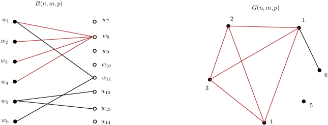
Figure 1: On the left, an example of $B(n,m,p)$ with $n=6$, $m=8$. On the right, the induced intersection graph $G(n,m,p)$. Observe that the red edges and the adjacent vertices on the left, which depicts a community with 4 members, induces a $K_{4}$ as subgraph (in red) on the right.

1 Background

In this work, we investigate the asymptotic behaviours of a critical random graph with non trivial clustering properties in its large-size limit. We carry out this investigation by identifying the scaling limit of the graph. By scaling limit, we are referring to a phenomenon in which the graph of size $n\in\mathbb{N}$, with its edge length rescaled to $a_{n}\in(0,\infty)$, converges in a suitable sense to a non trivial object as $n\to\infty$. Studying scaling limit of random graphs provides us with a panoramic perspective of the large-sized graphs, as well as direct access to global functionals including the diameters of the graphs. Meanwhile, as the current work shows, we can also gain insight into certain local functionals such as the numbers of triangles. Addario-Berry, Broutin and Goldschmidt [1] first identified the scaling limit of the Erdős–Rényi graph $G(n,p_{e})$, where each pair of vertices is independently connected by an edge with probability $p_{e}$. Since then, the focus has been on models of random graph with inhomogeneous degree sequences, a feature often shared by real-world networks. These include various versions of the inhomogeneous random graphs [5, 8, 9] and the configuration model [6, 11, 10]. On the other hand, clustering, another important aspect in the modelling of complex networks, has so far received little attention regarding its role in the scaling limit of random graphs. As a first attempt to fill this gap, our work investigates the question of existence of a scaling limit for the random intersection graph model introduced in Karoński et al. [20].

Let $n,m\in\mathbb{N}$ and $p\in[0,1]$. A random intersection graph with parameters $n,m,p$ can be obtained by first sampling a bipartite graph $B(n,m,p)$. More precisely, the vertex sets of this bipartite graph are denoted as $\mathcal{V}=\{w_{1},w_{2},\dots,w_{n}\}$ and $\mathcal{U}=\{w_{n+1},w_{n+2},\dots,w_{n+m}\}$, of respective sizes $n$ and $m$. Among the $nm$ possible edges between $\mathcal{V}$ and $\mathcal{U}$, each is present in $B(n,m,p)$ independently with probability $p$. It is often useful to think of $\mathcal{V}$-vertices (i.e. elements of $\mathcal{V}$) as individuals and $\mathcal{U}$-vertices as communities. The graph $B(n,m,p)$ can be then interpreted as a network model where each individual joins a community independently with probability $p$. The random intersection graph $G(n,m,p)$ induced by $B(n,m,p)$ is the graph on the vertex set $[n]:=\{1,2,3,\dots,n\}$ where two vertices $i,j$ are adjacent to each other in $G(n,m,p)$ if and only if the individuals they represent, i.e. $w_{i}$ and $w_{j}$, have joined a common community; see Fig. 1 for an example. In particular, we note that individuals from the same community are always adjacent to each other in $G(n,m,p)$; in other words, a community in $B(n,m,p)$ translates into a “clique”, i.e. a copy of complete graph, inside $G(n,m,p)$. This suggests that the local structure of $G(n,m,p)$ is not “tree-like”, unlike many random graphs studied previously.

Our main tool for studying $G(n,m,p)$ is a depth-first exploration of the bipartite graph $B(n,m,p)$, which allows us to extract a spanning forest from $B(n,m,p)$. Thanks to the criticality assumption, the question concerning the scaling limit of the graph largely reduces to identifying the scaling limit of this spanning forest. This, however, is still not a trivial question, as spanning forests that arise from the depth-first explorations of random graphs do not have “nice” distributional properties in general. Our approach, inspired by Conchon-Kerjan and Goldschmidt [10], relies on representing the spanning forest of $B(n,m,p)$ as a sequence of tilted Bienaymé trees.

Rest of the article is organised as follows. In Section 1.1, we introduce the relevant asymptotic regimes for the parameters of the model. In Section 1.2, we briefly review the result from [1] concerning the convergence of critical Erdős–Rényi graphs. The Erdős–Rényi case serves as a valuable benchmark in our study. We announce the main results in Section 2, whose proofs are found in Section 3.

1.1 Phase transition and clustering regimes

We are interested in how $G(n,m,p)$ behaves when both $n,m\to\infty$ and $p\sim\frac{c}{\sqrt{mn}}$ for some $c\in(0,\infty)$. Note in this case, the expected degree of any fixed vertex is given by

$$(n-1)\cdot\big{(}1-(1-p^{2})^{m}\big{)}\to c^{2},\quad\text{ as }n,m\to\infty.$$

It is shown in [4, 3] that the size of the largest connected component of $G(n,m,p)$ experiences a phase transition at $c=1$. In this work, we study the asymptotic behaviours of $G(n,m,p)$ in a regime around the criticality threshold $c=1$ called critical window. The analytic expression for the critical window of $G(n,m,p)$ depends, however, on the clustering regimes, a notion we are about to introduce. We refer to the following quantity as the clustering coefficient of $G(n,m,p)$:

$$\operatorname{CL}(G(n,m,p))=\mathbb{P}\big{(}\text{vertex $2$ adjacent to $3$}\,|\,\text{both $2,3$ adjacent to vertex $1$}\big{)}.$$

Clearly in above, $(1,2,3)$ can be replaced by any distinct triplet $(i,j,k)\in[n]^{3}$. In words, this is the probability of any three vertices forming a triangle knowing that they are already connected by edges. One can easily extend this definition of clustering coefficient to other graph models. In particular, for the Erdős–Rényi model $G(n,p_{e})$, we note its clustering coefficient is always equal to $p_{e}$, since edges there are drawn independently. In contrast, for the random intersection graph $G(n,m,p)$, assuming $p\sim\frac{1}{\sqrt{mn}}$, we can distinguish three different outcomes:

• If $\frac{m}{n}\to\infty$, then $\operatorname{CL}(G(n,m,p))\to 0$; this will be called the light clustering regime.

• If $\frac{m}{n}\to 0$, then $\operatorname{CL}(G(n,m,p))\to 1$; this will be called the heavy clustering regime.

• If $\frac{m}{n}\to\theta\in(0,\infty)$, then $\operatorname{CL}(G(n,m,p))\to(1+\sqrt{\theta})^{-1}\in(0,1)$; this will be called the moderate clustering regime.

Critical window in this article refers to the following sets of assumptions on $(m,n,p)$:

$$\frac{m}{n}\to\infty\quad\text{and}\quad p=\frac{1}{\sqrt{mn}}(1+\lambda n^{-\frac{1}{3}})\text{ for some $\lambda\in\mathbb{R}$}.$$ (L)

$$\exists\,\theta\in(0,\infty)\ \text{ s.t. }\ n^{\frac{1}{3}}\big{(}\tfrac{m}{n}-\theta\big{)}\to 0\ \text{ and }\ p=\frac{1}{\sqrt{mn}}(1+\lambda n^{-\frac{1}{3}})\text{ for some $\lambda\in\mathbb{R}$}.$$ (M)

$$\frac{m}{n}\to 0\quad\text{and}\quad p=\frac{1}{\sqrt{mn}}(1+\lambda m^{-\frac{1}{3}})\text{ for some $\lambda\in\mathbb{R}$}.$$ (H)

Let us mention that under (L) and (H), limit distributions for the component sizes of $G(n,m,p)$ have been investigated in Federico [14].

1.2 The continuum Erdős–Rényi graph

Before stating our results on the convergence of critical random intersection graphs, let us give a brief account on what happens in $G(n,p_{e})$. Assume $p_{e}=\frac{1}{n}(1+2\lambda n^{-1/3})$ for some $\lambda\in\mathbb{R}$. (The reason for the unconventional constant $2$ will become clearer shortly.) Denote by $G^{n}_{k}$ the $k$-th largest connected component of $G(n,p_{e})$. Let $d_{\operatorname{gr}}^{\mathrm{ER}}$ stand for the graph distance of $G(n,p_{e})$ and for $\alpha>0$, let $\alpha\cdot\mu^{\mathrm{ER}}_{k}$ be the finite measure which assigns a mass of $\alpha$ to each vertex of $G^{n}_{k}$. Equipped with the rescaled distance $n^{-1/3}\cdot d_{\operatorname{gr}}^{\mathrm{ER}}$ and the finite measure $n^{-2/3}\cdot\mu^{\mathrm{ER}}_{k}$, $(G^{n}_{k},d_{\operatorname{gr}}^{\mathrm{ER}},\mu^{\mathrm{ER}}_{k})$ is an instance of (random) measured metric space. It is shown in [1] that there exists a sequence of (random) measured metric spaces

$$\mathcal{G}^{\mathrm{ER}}(\lambda)=\big{\{}\big{(}\mathcal{C}^{\lambda,\infty}_{k},d^{\lambda,\infty}_{k},\mu^{\lambda,\infty}_{k}\big{)}:k\geq 1\big{\}}$$

so that the following convergence in distribution takes place as $n\to\infty$:

$$\Big{\{}\Big{(}G^{n}_{k},\,n^{-\frac{1}{3}}\cdot d_{\operatorname{gr}}^{\mathrm{ER}},\,n^{-\frac{2}{3}}\cdot\mu^{\mathrm{ER}}_{k}\Big{)}:k\geq 1\Big{\}}\;\Longrightarrow\;\mathcal{G}^{\mathrm{ER}}(\lambda)$$ (1)

We will come back to the construction of $\mathcal{G}^{\mathrm{ER}}(\lambda)$ in Section 2.3.2 and the precise meaning of the previous convergence in Section 2.4.

2 Main results

Recall (L), (M), (H), the assumptions of critical window in the respective light, moderate and heavy clustering regimes. For $k\geq 1$, we denote by $C^{n,m}_{k}$ the $k$-th largest connected component of $G(n,m,p)$. Denote by $d_{\operatorname{gr}}^{\mathrm{RIG}}$ the graph distance of $G(n,m,p)$. For $\alpha>0$, let $\alpha\cdot\mu^{\mathrm{RIG}}_{k}$ be the finite measure on $C^{n,m}_{k}$ which assigns a mass of $\alpha$ to each of its vertices.

Theorem 2.1 (Scaling limit in the moderate clustering regime).

Under the assumption (M), there exists a sequence of (random) measured metric spaces $\mathcal{G}^{\mathrm{RIG}}(\lambda,\theta)=\{(\mathcal{C}^{\lambda,\theta}_{k},d^{\lambda,\theta}_{k},\mu^{\lambda,\theta}_{k}):k\geq 1\}$ so that we have the following convergence in distribution as $n\to\infty$:

$$\Big{\{}\Big{(}C^{n,m}_{k},\,n^{-\frac{1}{3}}\cdot d_{\operatorname{gr}}^{\mathrm{RIG}},\,n^{-\frac{2}{3}}\cdot\mu^{\mathrm{RIG}}_{k}\Big{)}:k\geq 1\Big{\}}\;\Longrightarrow\;\mathcal{G}^{\mathrm{RIG}}(\lambda,\theta)$$ (2)

with respect to the weak convergence of the product topology induced by the Gromov–Hausdorff–Prokhorov topology.

Theorem 2.2 (Scaling limit in the light clustering regime).

Under the assumption (L), we have the following convergence in distribution as $n\to\infty$:

$$\Big{\{}\Big{(}C^{n,m}_{k},\,n^{-\frac{1}{3}}\cdot d_{\operatorname{gr}}^{\mathrm{RIG}},\,n^{-\frac{2}{3}}\cdot\mu^{\mathrm{RIG}}_{k}\Big{)}:k\geq 1\Big{\}}\;\Longrightarrow\;\mathcal{G}^{\mathrm{ER}}(\lambda)$$ (3)

with respect to the weak convergence of the product topology induced by the Gromov–Hausdorff–Prokhorov topology.

Theorem 2.3 (Scaling limit in the heavy clustering regime).

Under the assumption (H), we have the following convergence in distribution as $n\to\infty$:

$$\Big{\{}\Big{(}C^{n,m}_{k},\,m^{-\frac{1}{3}}\cdot d_{\operatorname{gr}}^{\mathrm{RIG}},\,m^{-\frac{1}{6}}n^{-\frac{1}{2}}\cdot\mu^{\mathrm{RIG}}_{k}\Big{)}:k\geq 1\Big{\}}\;\Longrightarrow\;\mathcal{G}^{\mathrm{ER}}(\lambda)$$ (4)

with respect to the weak convergence of the product topology induced by the Gromov–Hausdorff–Prokhorov topology.

To recap, in both light and heavy clustering regimes, we find the same limit object as in the critical Erdős–Rényi graph. However, the diameters of $C^{n,m}_{k}$ scale differently in these two regimes: as $m=o(n)$ under (H), Theorem 2.3 shows that the diameters are much smaller than those under (L) or those of critical $G(n,p_{e})$. In the moderate clustering regime, the scaling limit of $C^{n,m}_{k}$ belongs to a two-parameter family of measured metric spaces. As we will see in Section 2.3.3, $\mathcal{G}^{\mathrm{RIG}}(\lambda,\theta)$ still bears a strong affinity with the continuum Erdős–Rényi graph $\mathcal{G}^{\mathrm{ER}}(\lambda)$.

Let us recall that $G(n,m,p)$ is a deterministic function of the bipartite graph $B(n,m,p)$. Furthermore, there is a natural bijection between the vertex set $[n]$ of $G(n,m,p)$ and the vertex set $\mathcal{V}$ of $B(n,m,p)$ which maps $i\in[n]$ to $w_{i}\in\mathcal{V}$. Denote this bijection as $\rho_{n}$. Let $d_{\operatorname{gr}}^{\mathrm{bi}}$ stand for the graph distance of $B(n,m,p)$. Denote by $I_{k}$ the smallest vertex label in $C^{n,m}_{k}$ and let $\hat{C}^{n,m}_{k}$ be the connected component of $B(n,m,p)$ containing $w_{I_{k}}$, $k\geq 1$. Let $\mu^{\mathrm{bi}}_{k}$ be the measure of $\hat{C}^{n,m}_{k}$ that assigns a unit mass to each $\mathcal{V}$-vertex in $\hat{C}^{n,m}_{k}$. We write $\operatorname{\delta_{GHP}}$ for the Gromov–Hausdorff–Prokhorov distance between two measured metric space; see Section 2.3.1 for a formal definition. Let us point out the previous results on the scaling limit of $G(n,m,p)$ translates into analogous results for the bipartite graph $B(n,m,p)$, thanks to the following observation.

Proposition 2.4.

For all $n,m\in\mathbb{N}$, $\rho_{n}$ is an isometry from $([n],2\cdot d_{\operatorname{gr}}^{\mathrm{RIG}})$ to $(\mathcal{V},d_{\operatorname{gr}}^{\mathrm{bi}})$. As a result, the following holds almost surely for each $k\geq 1$:

$$\operatorname{\delta_{GHP}}\Big{(}\big{(}\hat{C}^{n,m}_{k},d_{\operatorname{gr}}^{\mathrm{bi}},\mu^{\mathrm{bi}}_{k}\big{)},\big{(}C^{n,m}_{k},2\cdot d_{\operatorname{gr}}^{\mathrm{RIG}},\mu^{\mathrm{RIG}}_{k}\big{)}\Big{)}\leq 1.$$

2.1 Convergence of the graph exploration processes

We obtain the aforementioned results on the scaling limit of $G(n,m,p)$ by studying certain stochastic processes that arise from a depth-first exploration of the bipartite graph $B(n,m,p)$. A related exploration of $G(n,m,p)$ appeared in [14]. Noting Proposition 2.4, which tells us that $B(n,m,p)$ will offer the same scaling limit as $G(n,m,p)$, we prefer to run the exploration on the bipartite graph as it contains additional information useful for triangle counts. We will use the following notation: for a vertex $w\in\mathcal{U}\cup\mathcal{V}$ of $B(n,m,p)$, we denote by

$$\mathcal{B}(w)=\{w^{\prime}\in\mathcal{U}\cup\mathcal{V}:d_{\operatorname{gr}}^{\mathrm{bi}}(w^{\prime},w)=1\},$$

the neighbourhood of $w$ in the graph. For a subgraph $G$ of $B(n,m,p)$, we write $\mathcal{V}(G)$ (resp. $\mathcal{U}(G)$) for the set of $\mathcal{V}$-vertices (resp. $\mathcal{U}$-vertices) contained in $G$; we also denote by $\mathcal{E}(G)$ the edge set of $G$. The following algorithm explores the neighbourhood of each vertex in a “depth-first” fashion, and outputs a spanning forest $\mathcal{F}$ of $B(n,m,p)$ in the end. To do so, the algorithm keeps track of the vertices that have not been explored at step $k$ using two subsets $\mathcal{V}_{k}$ and $\mathcal{U}_{k}$. The vertex explored at step $k$ is denoted as $v_{k}$, which is always a $\mathcal{V}$-vertex. There is a further subset of $\mathcal{V}$-vertices that do not belong to $\mathcal{V}_{k}$ nor to $\{v_{1},\dots,v_{k}\}$: these are the neighbours of the explored vertices whose neighbourhoods are yet to be explored; such a vertex is said to be active at step $k$. Information about active vertices are stored in an ordered list (i.e. sequence) $\mathcal{A}_{k}$, and the ordering in $\mathcal{A}_{k}$ determines which vertex to be explored next.

Algorithm 2.5 (Depth-first exploration of $B(n,m,p)$).

Initially, set $\mathcal{F}_{0}$ to be the empty graph and $\mathcal{A}_{0}=\mathcal{A}_{0}^{\ast}$ to be the empty sequence. Set $\mathcal{V}_{0}=\mathcal{V}_{0}^{\ast}=\mathcal{V}$ and $\mathcal{U}_{0}=\mathcal{U}$.

Step $k\geq 1$. If $\mathcal{A}^{\ast}_{k-1}=\varnothing$, let $v_{k}$ be a uniform element from $\mathcal{V}^{\ast}_{k-1}$; otherwise, let $v_{k}$ be the first element in $\mathcal{A}^{\ast}_{k-1}$. Set $\mathcal{V}_{k-1}=\mathcal{V}_{k-1}^{\ast}\setminus\{v_{k}\}$, and let $\mathcal{A}_{k-1}$ be the sequence obtained from $\mathcal{A}^{\ast}_{k-1}$ by removing $v_{k}$. Let

$$\mathcal{M}_{k}=\mathcal{B}(v_{k})\cap\mathcal{U}_{k-1}\quad\text{ and }\quad X^{n,m}_{k}=\#\mathcal{M}_{k}.$$

If $\mathcal{M}_{k}\neq\varnothing$, sort its elements in an increasing order of their labels and denote by $(u_{k,i})_{1\leq i\leq X^{n,m}_{k}}$ the sorted list. For $1\leq i\leq X^{n,m}_{k}$, define

$$\mathcal{N}_{k,i}=\mathcal{B}(u_{k,i})\cap\mathcal{V}_{k-1}\setminus\bigcup_{j=1}^{i-1}\mathcal{N}_{k,j}\quad\text{and}\quad\mathcal{N}_{k}=\bigcup_{1\leq i\leq X^{n,m}_{k}}\mathcal{N}_{k,i}.$$

Let $\mathcal{F}_{k}$ be the bipartite graph on the vertex sets $\mathcal{V}(\mathcal{F}_{k})=\mathcal{V}(\mathcal{F}_{k-1})\cup\{v_{k}\}\cup\mathcal{N}_{k}$ and $\mathcal{U}(\mathcal{F}_{k})=\mathcal{U}(\mathcal{F}_{k-1})\cup\mathcal{M}_{k}$ with its edge set given by

$$\mathcal{E}(\mathcal{F}_{k})=\mathcal{E}(\mathcal{F}_{k-1})\bigcup\big{\{}\{v_{k},u_{k,i}\}:1\leq i\leq X^{n,m}_{k}\big{\}}\bigcup\bigcup_{1\leq i\leq X^{n,m}_{k}}\big{\{}\{u_{k,i},v\}:v\in\mathcal{N}_{k,i}\big{\}}.$$

Set $\mathcal{V}_{k}^{\ast}=\mathcal{V}\setminus\mathcal{V}(\mathcal{F}_{k})=\mathcal{V}_{k-1}\setminus\mathcal{N}_{k}$ and $\mathcal{U}_{k}=\mathcal{U}\setminus\mathcal{U}(\mathcal{F}_{k})=\mathcal{U}_{k-1}\setminus\mathcal{M}_{k}$. If $\mathcal{N}_{k}$ is nonempty, sort its elements in an increasing order of their labels and add the ordered list to the top of $\mathcal{A}_{k-1}$; call the new sequence $\mathcal{A}^{\ast}_{k}$.

Stop when $\mathcal{V}_{k}^{\ast}=\varnothing$. Add each member of $\mathcal{U}_{k}$ to $\mathcal{F}_{k}$ as an isolated vertex; call the resulting graph $\mathcal{F}$.

We note that the algorithm always terminates at step $n$, when all the $\mathcal{V}$-vertices are explored. Moreover, for each $1\leq k\leq n$, the sets $\mathcal{N}_{k,i},1\leq i\leq X^{n,m}_{k}$, are pairwise disjoint. Note also that $\mathcal{F}_{k}$ is loop-free, and consequently the final graph $\mathcal{F}$ is a spanning forest of $B(n,m,p)$. In particular, each connected component of $\mathcal{F}$ is a spanning tree of a connected component of $B(n,m,p)$. If a connected component of $\mathcal{F}$ contains more than one vertex, then it must contain some $v_{k}$ and root the tree at the $v_{k}$ with the smallest $k$; otherwise, root the tree at the sole vertex.

Figure 2: Upper left: an example of $B(n,m,p)$ and its exploration; dashed edges are those not in the spanning forest. Upper right: the corresponding $S^{n,m}$. Lower left: the corresponding $R^{n,m}$. Lower right: the corresponding $H^{n,m}$. The successive values of $\#\mathcal{N}_{k}$ are $3,2,0,0,0,0,1,2,0,0$; the values of $\#\mathcal{M}_{k}$ are resp. $2,1,0,0,0,0,1,2,0,0$. The values of $\#\mathcal{A}_{k}$ are resp. $2,3,2,1,0,0,0,1,0,0$.

The following stochastic processes are the key tools in our study of $B(n,m,p)$ and $G(n,m,p)$. Set $R^{n,m}_{0}=S^{n,m}_{0}=0$. For $k\geq 1$, let

$$R^{n,m}_{k}-R^{n,m}_{k-1}=\#\mathcal{M}_{k},\quad S^{n,m}_{k}-S^{n,m}_{k-1}=\#\mathcal{N}_{k}-1.$$ (5)

Meanwhile, for a sequence of integers $(s_{j})_{0\leq j\leq k}$, we define

$$\mathscr{H}_{k}\big{(}(s_{j})_{0\leq j\leq k}\big{)}=\#\Big{\{}0\leq j\leq k-1:s_{j}=\min_{j\leq i\leq k-1}s_{i}\Big{\}}.$$ (6)

We then set

$$H^{n,m}_{k}=\mathscr{H}_{k}((S^{n,m}_{j})_{0\leq j\leq k}),\quad k\geq 1.$$

We say the height of a vertex $v$ in $\mathcal{F}$ is the graph distance from $v$ to the root of the tree component of $\mathcal{F}$ that contains $v$. The usefulness of $H^{n,m}:=(H^{n,m}_{k})_{k\geq 1}$ lies in the following property, whose proof is found towards the end of Section 3.1.

Lemma 2.6.

For $n\in\mathbb{N}$ and $1\leq k\leq n$, $2H^{n,m}_{k}-2$ is the height of $v_{k}$ in $\mathcal{F}$.

We will refer to the pair $(R^{n,m},S^{n,m}):=(R^{n,m}_{k},S^{n,m}_{k})_{k\geq 0}$ as the depth-first walk of $B(n,m,p)$, and $(H^{n,m}_{k})_{k\geq 0}$ as the height process; see Fig. 2 for an example. Unlike usual height processes, our definition of $H^{n,m}$ only pertains to vertices at even heights. This is however sufficient for our purpose as the rest of $\mathcal{F}$ are at distance 1 from those vertices. The triplet $(R^{n,m},S^{n,m},H^{n,m})$ forms the graph exploration process for $B(n,m,p)$ and their scaling limit is our next focus.

Let $(W_{t})_{t\geq 0},(W^{\ast}_{t})_{t\geq 0}$ be two independent standard linear Brownian motions. Denote $\mathbb{R}_{+}=[0,\infty)$. For a closed interval $I\subseteq\mathbb{R}_{+}$ and $d\in\mathbb{N}$, let $\mathbb{C}(I,\mathbb{R}^{d})$ be the set of all continuous maps from $I$ to $\mathbb{R}^{d}$, equipped with the uniform topology.

Proposition 2.7 (Convergence of the exploration processes in the light clustering regime).

Under the assumption (L), we have the following convergence in distribution in $\mathbb{C}(\mathbb{R}_{+},\mathbb{R}^{3})$:

$$\Big{\{}n^{-\frac{1}{6}}m^{-\frac{1}{2}}R^{n,m}_{\lfloor n^{2/3}t\rfloor},n^{-\frac{1}{3}}S^{n,m}_{\lfloor n^{2/3}t\rfloor},n^{-\frac{1}{3}}H^{n,m}_{\lfloor n^{2/3}t\rfloor}:t\geq 0\Big{\}}\Longrightarrow\Big{\{}t,\mathcal{S}^{\lambda,\infty}_{t},\mathcal{H}^{\lambda,\infty}_{t}:t\geq 0\Big{\}},$$ (7)

where the limit processes $\mathcal{S}^{\lambda,\infty}=(\mathcal{S}^{\lambda,\infty}_{t})_{t\geq 0},\mathcal{H}^{\lambda,\infty}=(\mathcal{H}^{\lambda,\infty}_{t})_{t\geq 0}$ are defined as follows:

$$\mathcal{S}^{\lambda,\infty}_{t}=W_{t}+2\lambda t-\tfrac{1}{2}t^{2},\quad\mathcal{H}^{\lambda,\infty}_{t}=2\Big{(}\mathcal{S}^{\lambda,\infty}_{t}-\min_{s\leq t}\mathcal{S}^{\lambda,\infty}_{s}\Big{)},\quad t\geq 0.$$

Proposition 2.8 (Convergence of the exploration processes in the moderate clustering regime).

Assume (M). Let $\tilde{R}^{n,m}_{k}=R^{n,m}_{k}-\sqrt{\theta}k$, $k\geq 1$. We have the following convergence in distribution in $\mathbb{C}(\mathbb{R}_{+},\mathbb{R}^{3})$:

$$\Big{\{}n^{-\frac{1}{3}}\tilde{R}^{n,m}_{\lfloor n^{2/3}t\rfloor},n^{-\frac{1}{3}}S^{n,m}_{\lfloor n^{2/3}t\rfloor},n^{-\frac{1}{3}}H^{n,m}_{\lfloor n^{2/3}t\rfloor}:t\geq 0\Big{\}}\Longrightarrow\Big{\{}\mathcal{R}^{\lambda,\theta}_{t},\mathcal{S}^{\lambda,\theta}_{t},\mathcal{H}^{\lambda,\theta}_{t}:t\geq 0\Big{\}},$$ (8)

where the limit processes $(\mathcal{R}^{\lambda,\theta},\mathcal{S}^{\lambda,\theta})=(\mathcal{R}^{\lambda,\theta}_{t},\mathcal{S}^{\lambda,\theta}_{t})_{t\geq 0},\mathcal{H}^{\lambda,\theta}=(\mathcal{H}^{\lambda,\theta}_{t})_{t\geq 0}$ are defined as follows:

$$\mathcal{R}^{\lambda,\theta}_{t}=\theta^{\frac{1}{4}}W^{\ast}_{t}+\theta^{\frac{1}{2}}\lambda t-\tfrac{1}{2}t^{2},\quad\mathcal{S}^{\lambda,\theta}_{t}=W_{t}+\theta^{-\frac{1}{4}}W^{\ast}_{t}+2\lambda t-\tfrac{1}{2}(1+\theta^{-\frac{1}{2}})t^{2},\ \text{ and }$$ (9)

$$\mathcal{H}^{\lambda,\theta}_{t}=\frac{2}{1+\theta^{-\frac{1}{2}}}\Big{(}\mathcal{S}^{\lambda,\theta}_{t}-\min_{s\leq t}\mathcal{S}^{\lambda,\theta}_{s}\Big{)}.$$ (10)

The process $(\mathcal{H}^{\lambda,\infty}_{t})_{t\geq 0}$ (resp. $(\mathcal{H}^{\lambda,\theta}_{t})_{t\geq 0}$) is the height process of $(\mathcal{S}^{\lambda,\infty}_{t})_{t\geq 0}$ (resp. of $(\mathcal{S}^{\lambda,\theta}_{t})_{t\geq 0}$). We point to Sections 2.3.2 and 2.3.3 for further information on their definitions. Let us also note that by letting $\theta\to\infty$ in the expression of $\mathcal{S}^{\lambda,\theta}_{t}$, we recover $\mathcal{S}^{\lambda,\infty}_{t}$, which motivates our notation.

From the definition of $B(n,m,p)$, it is clear that exchanging the roles of $n$ and $m$ leaves the distribution of the graph unchanged. By running Algorithm 2.5 on $B(m,n,p)$ instead of $B(n,m,p)$ and letting $(R^{m,n}_{k},S^{m,n}_{k})_{k\geq 0},(H^{m,n}_{k})_{k\geq 0}$ be the corresponding depth-first walk and height process, Proposition 2.7 has as immediate consequence as follows.

Corollary 2.9 (Convergence of the exploration processes in the heavy clustering regime).

Under Assumption (H), the following convergence in distribution holds in $\mathbb{C}(\mathbb{R}_{+},\mathbb{R}^{3})$:

$$\Big{\{}m^{-\frac{1}{6}}n^{-\frac{1}{2}}R^{m,n}_{\lfloor m^{2/3}t\rfloor},m^{-\frac{1}{3}}S^{m,n}_{\lfloor m^{2/3}t\rfloor},m^{-\frac{1}{3}}H^{m,n}_{\lfloor m^{2/3}t\rfloor}:t\geq 0\Big{\}}\Longrightarrow\Big{\{}t,\mathcal{S}^{\lambda,\infty}_{t},\mathcal{H}^{\lambda,\infty}_{t}:t\geq 0\Big{\}},$$ (11)

where $\mathcal{S}^{\lambda,\infty}_{t},\mathcal{H}^{\lambda,\infty}_{t}$ are the same as in Proposition 2.7.

Proof of Propositions 2.7 and 2.8 will occupy a major part of Section 3.

2.2 Triangle counts and surplus edges

Given a connected graph $G$ and a spanning tree $T$ of $G$, we say an edge $e$ of $G$ is a surplus edge if it is not present in $T$. Although the notion of surplus edge depends on the spanning tree, the number of surplus edges does not and is given by $\#E(G)-\#G+1$, where $\#E(G)$ stands for the number of edges in $G$ and $\#G$ counts the number of vertices in $G$. In a nutshell, results here tell us that large connected components of the critical bipartite graph $B(n,m,p)$ contain very few surplus edges even as their sizes tend to infinity, which is reminiscent of the situation for critical Erdős–Rényi graphs ([2, 1]). In contrast, as we will see in Theorems 2.12-2.14 below, $G(n,m,p)$ can exhibit a range of behaviours regarding surplus edges. Nevertheless, the presence of these surplus edges in $G(n,m,p)$ does not change significantly the metric aspect of the graph, as indicated in Proposition 2.4.

Let us start with the bipartite graph $B(n,m,p)$. From now on, we will refer to an edge of $B(n,m,p)$ as a (bipartite) surplus edge if it is not contained in the spanning forest $\mathcal{F}$ from Algorithm 2.5. We will need information on the distribution of these bipartite surplus edges to identify the scaling limit of $B(n,m,p)$. Let us denote by $\mathcal{E}^{\mathrm{S}}(n,m)$ the set of surplus edges of $B(n,m,p)$. Recall from Algorithm 2.5 the sets $\mathcal{M}_{k},\mathcal{A}_{k},\mathcal{N}_{k,i}$. We have the following description of $\mathcal{E}^{\mathrm{S}}(n,m)$.

Lemma 2.10.

If $e=\{u,w\}\in\mathcal{E}^{\mathrm{S}}(n,m)$, then there is a unique $k\in[n]$ so that one of the two following cases occurs:

1. either $u\in\mathcal{M}_{k}$ and $w\in\mathcal{A}_{k-1}$;

2. or there exists $1\leq i<j\leq\#\mathcal{M}_{k}$ satisfying $w\in\mathcal{N}_{k,i}$ and $u=u_{k,j}$.

Proof for Lemma 2.10 is short; we therefore include it here. See also the example illustrated in Fig. 2.

Proof.

Since $\mathcal{M}_{k},k\in[n]$, are disjoint and $\cup_{k\in[n]}\mathcal{M}_{k}$ comprises all non isolated $\mathcal{U}$-vertices, there must be a unique $k\in\mathbb{N}$ satisfying $u\in\mathcal{M}_{k}$. In that case, we must have the neighbourhood $\mathcal{B}(u)$ of $u$ contained in $\mathcal{N}_{k}\cup\mathcal{A}_{k-1}\cup\{v_{k}\}$. However, if $w=v_{k}$, then $e=\{u,w\}$ would be an edge of $\mathcal{F}$. So $w$ belongs to either $\mathcal{A}_{k-1}$ or $\mathcal{N}_{k}$. In the latter case, as the edge $e$ is not present in $\mathcal{F}$, it can only happen when $w$ is adjacent to at least two elements of $\mathcal{M}_{k}$. ∎

To study the limit distribution of $\mathcal{E}^{\mathrm{S}}(n,m)$, we first turn it into a point measure as follows. For $e=\{u,w\}\in\mathcal{E}^{\mathrm{S}}(n,m)$, let $k(e)$ be the unique $k\in[n]$ identified in Lemma 2.10. If $w\in\mathcal{A}_{k-1}$, recalling that $\mathcal{A}_{k-1}$ is an ordered list, we let $l(e)$ be the rank of the element $w$ in $\mathcal{A}_{k-1}$. If $w\notin\mathcal{A}_{k-1}$, we set $l(e)=0$. We introduce the following point measure on $\mathbb{R}^{2}$:

$$\tilde{P}^{n,m}(dx,dy)=\sum_{e\in\mathcal{E}^{\mathrm{S}}(n,m)}\delta_{(n^{-2/3}k(e),\,n^{-1/3}l(e))}.$$ (12)

We note that $\tilde{P}^{n,m}$ is not necessarily simple, i.e. it may contain multiple atoms at the same location. We let $P^{n,m}$ be the simple point measure with the same support as $\tilde{P}^{n,m}$. Given $\mathcal{F}$ and $P^{n,m}$, we will construct in Section 3.7 a graph that has the same scaling limit as $B(n,m,p)$. To describe the limit of $P^{n,m}$, we need the following objects. Recall from Propositions 2.7 and 2.8 the processes $\mathcal{S}^{\lambda,\infty}$ and $(\mathcal{R}^{\lambda,\theta},\mathcal{S}^{\lambda,\theta})$. Conditional on $\mathcal{S}^{\lambda,\infty}$, let $\mathcal{P}^{\lambda,\infty}$ be a Poisson point measure on $\mathbb{R}^{2}$ with intensity measure $dxdy\mathbf{1}_{\{(x,y)\in\mathcal{D}^{\lambda,\infty}\}}$, where

$$\mathcal{D}^{\lambda,\infty}=\big{\{}(x,y):x\in\mathbb{R}_{+},0\leq y\leq\mathcal{S}^{\lambda,\infty}_{x}-\min_{u\leq x}\mathcal{S}^{\lambda,\infty}_{u}\big{\}}.$$

Similarly, conditional on $(\mathcal{R}^{\lambda,\theta},\mathcal{S}^{\lambda,\theta})$, let $\mathcal{P}^{\lambda,\theta}$ be a Poisson point measure on $\mathbb{R}^{2}$ with intensity measure $dxdy\mathbf{1}_{\{(x,y)\in\mathcal{D}^{\lambda,\theta}\}}$, where

$$\mathcal{D}^{\lambda,\theta}=\big{\{}(x,y):x\in\mathbb{R}_{+},0\leq y\leq\mathcal{S}^{\lambda,\theta}_{x}-\min_{u\leq x}\mathcal{S}^{\lambda,\theta}_{u}\big{\}}.$$

Proposition 2.11 (Convergence of the bipartite surplus edges).

Under the assumption (L), jointly with the convergence (7) in Proposition 2.7, we have the weak convergence of the random measure $P^{n,m}$ to $\mathcal{P}^{\lambda,\infty}$ on every compact set of $\mathbb{R}^{2}$. Under the assumption (M), jointly with the convergence (8) in Proposition 2.8, we have the weak convergence of the random measure $\mathcal{P}^{n,m}$ to $\mathcal{P}^{\lambda,\theta}$ on every compact set of $\mathbb{R}^{2}$.

Proof of Proposition 2.11 is given in Section 3.6. We now turn our attention to the random intersection graph $G(n,m,p)$. Let us denote by $\mathrm{L}^{n,m}_{k}$ the number of triangles in the $k$-th largest connected component of $G(n,m,p)$, noting that each triangle must contain at least one surplus edge. Recall that the excursions of $\mathcal{S}^{\lambda,\infty}$ above its running infimum can be ranked in a decreasing order of their lengths, as shown by Aldous in [2]. This also holds true for $\mathcal{S}^{\lambda,\theta}$; see Section 2.3.3. Hence, for $\theta\in(0,\infty)\cup\{\infty\}$ and $k\in\mathbb{N}$, we can define

$$\zeta^{\lambda,\theta}_{k}=\text{length of the $k$-th longest excursion of }\big{(}\mathcal{S}^{\lambda,\theta}_{t}-\min_{s\leq t}\mathcal{S}^{\lambda,\theta}_{s}\big{)}_{t\geq 0}.$$ (13)

Theorem 2.12 (Triangle counts in the moderate clustering regime).

Under the assumption (M), for each $k\geq 1$, we have the following joint convergence in distribution

$$n^{-\frac{2}{3}}\cdot\big{(}\mathrm{L}^{n,m}_{1},\mathrm{L}^{n,m}_{2},\mathrm{L}^{n,m}_{3},\cdots,\mathrm{L}^{n,m}_{k}\big{)}\ \Longrightarrow\ c_{\theta}\cdot\big{(}\zeta^{\lambda,\theta}_{1},\zeta^{\lambda,\theta}_{2},\zeta^{\lambda,\theta}_{3},\cdots,\zeta^{\lambda,\theta}_{k}\big{)}.$$

The constant $c_{\theta}$ is given by

$$c_{\theta}=\frac{1}{2\sqrt{\theta}}+\frac{1}{6\theta}=\frac{\sqrt{\theta}}{6}\mathbb{E}\Big{[}(X_{\theta}+1)X_{\theta}(X_{\theta}-1)\Big{]},$$ (14)

where $X_{\theta}$ stands for a Poisson random variable of expectation $\sqrt{\theta}^{-1}$.

Theorem 2.13 (Triangle counts in the light clustering regime).

Under the assumption (L), the following statements hold true.

1. If $\frac{m}{n^{7/3}}\to 0$ as $n\to\infty$, then for each $k\geq 1$, we have the following joint convergence in distribution

   $$m^{\frac{1}{2}}n^{-\frac{7}{6}}\cdot\big{(}\mathrm{L}^{n,m}_{1},\mathrm{L}^{n,m}_{2},\mathrm{L}^{n,m}_{3},\cdots,\mathrm{L}^{n,m}_{k}\big{)}\ \Longrightarrow\ \big{(}\tfrac{1}{2}\zeta^{\lambda,\infty}_{1},\tfrac{1}{2}\zeta^{\lambda,\infty}_{2},\tfrac{1}{2}\zeta^{\lambda,\infty}_{3},\cdots,\tfrac{1}{2}\zeta^{\lambda,\infty}_{k}\big{)}.$$

2. If $\frac{m}{n^{7/3}}\to\infty$ as $n\to\infty$, then for each $k\geq 1$, we have

   $$\max_{j\leq k}\mathrm{L}^{n,m}_{j}\longrightarrow 0\quad\text{ in probability}.$$

3. If $m=\lfloor n^{7/3}\rfloor$, then for each $k\geq 1$, we have the joint convergence in distribution:

   $$\big{(}\mathrm{L}^{n,m}_{1},\mathrm{L}^{n,m}_{2},\mathrm{L}^{n,m}_{3},\cdots,\mathrm{L}^{n,m}_{k}\big{)}\ \Longrightarrow\ \big{(}\mathcal{L}_{1},\mathcal{L}_{2},\mathcal{L}_{3},\cdots,\mathcal{L}_{k}\big{)},$$

   where conditional on $\mathcal{S}^{\lambda,\infty}$, $(\mathcal{L}_{i})_{1\leq i\leq k}$ is a collection of independent Poisson variables with respective expectations $\tfrac{1}{2}\zeta^{\lambda,\infty}_{i}$, $1\leq i\leq k$.

Theorem 2.14 (Triangle counts in the heavy clustering regime).

Under the assumption (H), for each $k\geq 1$, we have the following joint convergence in distribution

$$m^{\frac{5}{6}}n^{-\frac{3}{2}}\cdot\big{(}\mathrm{L}^{n,m}_{1},\mathrm{L}^{n,m}_{2},\mathrm{L}^{n,m}_{3},\cdots,\mathrm{L}^{n,m}_{k}\big{)}\ \Longrightarrow\ \big{(}\tfrac{1}{6}\zeta^{\lambda,\infty}_{1},\tfrac{1}{6}\zeta^{\lambda,\infty}_{2},\tfrac{1}{6}\zeta^{\lambda,\infty}_{3},\cdots,\tfrac{1}{6}\zeta^{\lambda,\infty}_{k}\big{)}.$$

Proof of Theorems 2.12 and 2.13 is found in Section 3.8 and proof of Theorem 2.14 in Section 3.9.

2.3 Construction of the limit graphs

After a quick recap on some topological notions, we explain here the constructions of $\mathcal{G}^{\mathrm{ER}}(\lambda)$ and $\mathcal{G}^{\mathrm{RIG}}(\lambda,\theta)$ from the Brownian motion.

2.3.1 Graphs encoded by real-valued functions

We follow the approaches in [1, 8], with some minor differences in detail. The account we give here relies on the notions of real tree [13], measured metric space [16], and Gromov–Hausdorff–Prokhorov topology [25], which are now standard. We therefore point to the previous references for their definitions and further background. We first recall the construction of a real tree from a real-valued function. Let $\zeta_{h}\in(0,\infty)$ and suppose that $h:[0,\zeta_{h}]\to\mathbb{R}_{+}$ is a continuous function. The following symmetric function

$$d_{h}(s,t):=h(s)+h(t)-2b_{h}(s,t),\quad\text{where}\quad b_{h}(s,t)=\min\{h(u):\min(s,t)\leq u\leq\max(s,t)\}$$

defines a pseudo-distance on $[0,\zeta_{h}]$. To turn it into a distance, we introduce an equivalence relation by defining $s\sim_{h}t$ if and only if $d_{h}(s,t)=0$. Then $d_{h}$ induces a distance on the quotient space $T_{h}:=[0,\zeta_{h}]/\sim_{h}$, which we still denote as $d_{h}$. Moreover, the compact metric space $(T_{h},d_{h})$ has the property that every pair of points in it is joined by a unique path which is also geodesic. In other words, $(T_{h},d_{h})$ is a real tree. Let $p_{h}$ stand for the canonical projection from $[0,\zeta_{h}]$ to $T_{h}$ and denote by $\mu_{h}$ the push-forward of the Lebesgue measure on $[0,\zeta_{h}]$ by $p_{h}$. Set

$$\mathcal{T}_{h}:=\big{(}T_{h},d_{h},\mu_{h}\big{)}.$$ (15)

For two points $x,y$ from $T_{h}$, let us write $\llbracket x,y\rrbracket$ for the unique path in $T_{h}$ from $x$ to $y$, whose length is given by $d_{h}(x,y)$. Suppose that $q\in\mathbb{N}$ and $\Pi=\{(s_{i},t_{i}):1\leq i\leq q\}$ is a collection satisfying $0\leq s_{i}\leq t_{i}\leq\zeta_{h}$ for $1\leq i\leq q$. Their images in $T_{h}$ are denoted as

$$x_{i}=p_{h}(s_{i}),\quad y_{i}=p_{h}(t_{i}),\quad 1\leq i\leq q.$$

For a pair of $(x,y)\in T_{h}^{2}$, we define a set $\Gamma_{\Pi}^{x,y}$ formed by sequences of paths that take the following form:

$$\boldsymbol{\gamma}=\big{(}\llbracket u_{1},u_{2}\rrbracket,\llbracket u_{3},u_{4}\rrbracket,\dots,\llbracket u_{2\ell-1},u_{2\ell}\rrbracket\big{)}\,,$$

where $\ell\in\mathbb{N}$, $u_{1}=x,u_{2\ell}=y$, $u_{2j}\in\{x_{i}:1\leq i\leq q\}$, and if $u_{2j}=x_{i}$, then $u_{2j+1}=y_{i}$, for $1\leq j\leq\ell-1$. For such a $\boldsymbol{\gamma}=\big{(}\llbracket u_{2j-1},u_{2j}\rrbracket\big{)}_{1\leq j\leq\ell}$, we define its $\Pi$-modified length as follows:

$$\ell_{\Pi}(\boldsymbol{\gamma})=\sum_{j=1}^{\ell}d_{h}(u_{2j-1},u_{2j}).$$

The following defines a pseudo-distance on $T_{h}$: for all $x,y\in T_{h}$, let

$$d_{h,\Pi}(x,y)=\inf\big{\{}\ell_{\Pi}(\boldsymbol{\gamma}):\boldsymbol{\gamma}\in\Gamma_{\Pi}^{x,y}\big{\}}.$$

As previously, we can turn it into a true distance by quotienting the points at $d_{h,\Pi}$-distance 0 from each other. Call the resulting metric space $(G_{h,\Pi},d_{h,\Pi})$ and denote by $p_{h,\Pi}$ the canonical projection from $(T_{h},d_{h})$ to $(G_{h,\Pi},d_{h,\Pi})$. Write $\mu_{h,\Pi}$ for the push-forward of $\mu_{h}$ by $p_{h,\Pi}$. Finally, let us denote

$$\mathcal{G}(h,\Pi)=\big{(}G_{h,\Pi},d_{h,\Pi},\mu_{h,\Pi}\big{)},$$ (16)

which is a measured metric space. Recall that two measured metric spaces, say $\mathcal{G}_{1}=(G_{1},d_{1},\mu_{1})$ and $\mathcal{G}_{2}=(G_{2},d_{2},\mu_{2})$, can be compared using their Gromov–Hausdorff–Prokhorov distance:

$$\operatorname{\delta_{GHP}}(\mathcal{G}_{1},\mathcal{G}_{2}):=\inf\big{\{}\operatorname{d^{\mathrm{Haus}}_{E}}\big{(}\phi_{1}(G_{1}),\phi_{2}(G_{2})\big{)}+\operatorname{d^{\mathrm{Pr}}_{E}}\big{(}\mu_{1}\circ\phi_{1}^{-1},\mu_{2}\circ\phi_{2}^{-1}\big{)}\big{\}},$$

where the infimum is over all Polish spaces $(E,d_{E})$ and isometric embeddings $\phi_{i}$ from $G_{i}\to E$; $\operatorname{d^{\mathrm{Haus}}_{E}}$ stands for the Hausdorff distance of $E$, and $\operatorname{d^{\mathrm{Pr}}_{E}}$ is the Prokhorov distance for the finite Borel measures on $E$, with $\mu_{i}\circ\phi_{i}^{-1}$ standing for the push-forward of $\mu_{i}$ by $\phi_{i}$, $i=1,2$. We further point out that the space of (equivalence classes) of compact measured metric spaces is a Polish space in the topology induced by $\operatorname{\delta_{GHP}}$ ([25]). The following statement, taken from [8], provides a practical way to prove Gromov–Hausdorff–Prokhorov convergence for measured metric spaces that are constructed from real-valued functions as described above. Let $q\in\mathbb{N}$. For $j\in\{1,2\}$, suppose that $h_{j}:[0,\zeta_{j}]\to\mathbb{R}_{+}$ is a continuous function and $\Pi_{j}=\{(s_{j,i},t_{j,i}):1\leq i\leq q\}$ is a collection of points with $0\leq s_{j,i}\leq t_{j,i}<\zeta_{j}$ for each $j\leq q$. Suppose further that there is some $\delta>0$ verifying

$$\max_{1\leq i\leq q}|s_{1,i}-s_{2,i}|\leq\delta,\quad\max_{1\leq i\leq q}|t_{1,i}-t_{2,i}|\leq\delta.$$

Then we have ([8], Lemma 2.7)

$$\operatorname{\delta_{GHP}}\big{(}\mathcal{G}(h_{1},\Pi_{1}),\mathcal{G}(h_{2},\Pi_{2})\big{)}\leq 6(p+1)\big{(}\|\hat{h}_{1}-\hat{h}_{2}\|_{\infty}+\omega_{\delta}(\hat{h}_{1})\big{)}+|\zeta_{1}-\zeta_{2}|,$$ (17)

where $\hat{h}_{j}$ is the extension of $h_{j}$ to $\mathbb{R}_{+}$ by setting $\hat{h}_{j}(x)=0$ for all $x\geq\zeta_{j}$, and $\omega_{\delta}(h_{1})=\sup\{|h_{1}(s)-h_{1}(t)|:|s-t|\leq\delta\}$ is the $\delta$-modulus of continuity of $h_{1}$.

2.3.2 The continuum Erdős–Rényi graph

We recall from Proposition 2.7 the stochastic process $\mathcal{S}^{\lambda,\infty}$ and its height process $\mathcal{H}^{\lambda,\infty}$:

$$\mathcal{S}^{\lambda,\infty}_{t}=W_{t}+2\lambda t-\tfrac{1}{2}t^{2},\quad\mathcal{H}^{\lambda,\infty}_{t}=2\Big{(}\mathcal{S}^{\lambda,\infty}_{t}-\min_{s\leq t}\mathcal{S}^{\lambda,\infty}_{s}\Big{)},$$

where $(W_{t})_{t\geq 0}$ is a standard linear Brownian motion. As Proposition 2.7 indicates, the pair $(\mathcal{S}^{\lambda,\infty},\mathcal{H}^{\lambda,\infty})$ is a continuum analogue for $(S^{n,m}_{k},H^{n,m}_{k})_{k\geq 0}$, the discrete depth-first walk and its height process. We also recall the identity (6), which expresses $(H^{n,m}_{k})_{k\geq 0}$ as a deterministic function of $(S^{n,m}_{k})_{k\geq 0}$. As it turns out, there is an analogue of (6) for spectrally positive Lévy processes, discovered by Le Gall and Le Jan [23]. Roughly speaking, if $X=(X_{t})_{t\geq 0}$ a spectrally positive Lévy process, then for $t>0$, the following limit exists in probability:

$$\mathcal{H}^{X}_{t}=\lim_{\epsilon\to 0}\frac{1}{\epsilon}\int_{0}^{t}\mathbf{1}_{\{X_{s}\leq\inf_{s\leq u\leq t}X_{u}+\epsilon\}}ds,$$

leading to the definition of a height process for $X$; see [12, 23] for more detail. However, in the special case where $X=(c\cdot W_{t})_{t\geq 0}$ for some $c>0$, it turns out that

$$\mathcal{H}^{X}_{t}=\frac{2}{c^{2}}\Big{(}X_{t}-\min_{s\leq t}X_{s}\Big{)}\quad\text{a.s.}$$ (18)

for each $t$. This is discovered in [24]; see also Eq. (1.7) in [12]. The identity then extends to $\mathcal{S}^{\lambda,\infty}$ by Girsanov’s Theorem, which explains the expression of $\mathcal{H}^{\lambda,\infty}$ as seen above.

We can now give an explicit construction of $\mathcal{G}^{\mathrm{ER}}(\lambda)$ that appears in the scaling limit of critical $G(n,p_{e})$ ([1]) as well as of critical $G(n,m,p)$ in the light and heavy clustering regimes. For $t>0$, let $g(t)$ (resp. $d(t)$) be the last zero of $\mathcal{H}^{\lambda,\infty}$ before $t$ (resp. first zero of $\mathcal{H}^{\lambda,\infty}$ after $t$). Alternatively, $(g(t),d(t))$ is the excursion interval of $\mathcal{S}^{\lambda,\infty}$ above its running infimum that contains $t$. It is shown in [2] that $d(t)-g(t)\to 0$ in probability as $t\to\infty$. Consequently, we can rank the excursions of $\mathcal{H}^{\lambda,\infty}$ above $0$ in a decreasing order of their lengths. For $k\geq 1$, let $(\mathrm{g}^{\lambda,\infty}_{k},\mathrm{d}^{\lambda,\infty}_{k})$ be the $k$-th longest such excursion interval, which is unique almost surely. Recall $\zeta^{\lambda,\infty}_{k}$ from (13); we have $\zeta^{\lambda,\infty}_{k}=\mathrm{d}^{\lambda,\infty}_{k}-\mathrm{g}^{\lambda,\infty}_{k}$. The excursion of $\mathcal{H}^{\lambda,\infty}$ running on the interval $(\mathrm{g}^{\lambda,\infty}_{k},\mathrm{d}^{\lambda,\infty}_{k})$ is denoted as $\mathrm{e}^{\lambda,\infty}_{k}$, namely,

$$e^{\lambda,\infty}_{k}:[0,\zeta^{\lambda,\infty}_{k}]\to\mathbb{R}_{+}\quad\text{with}\quad e^{\lambda,\infty}_{k}(s)=\mathcal{H}^{\lambda,\infty}_{s+\mathrm{g}^{\lambda,\infty}_{k}}.$$

Recall from Proposition 2.11 the Poisson point process $\mathcal{P}^{\lambda,\infty}$ on $\mathbb{R}^{2}$, which has a finite number of atoms on every $(a,b)\times\mathbb{R}$ for $0\leq a<b<\infty$. Let

$$p^{\lambda,\infty}_{k}=\#\mathcal{P}^{\lambda,\infty}\cap(\mathrm{g}^{\lambda,\infty}_{k},\mathrm{d}^{\lambda,\infty}_{k})\times\mathbb{R}\,,$$

and write $\{(x_{k,i},y_{k,i}):1\leq i\leq p^{\lambda,\infty}_{k}\}$ for the elements in $\mathcal{P}^{\lambda,\infty}\cap(\mathrm{g}^{\lambda,\infty}_{k},\mathrm{d}^{\lambda,\infty}_{k})\times\mathbb{R}$. By the definition of $\mathcal{P}^{\lambda,\infty}$, we have a.s.

$$0<y_{k,i}\leq\mathcal{S}^{\lambda,\infty}_{x_{k,i}}-\min_{u\leq x_{k,i}}\mathcal{S}^{\lambda,\infty}_{u},\quad 1\leq i\leq p^{\lambda,\infty}_{k}.$$

For $1\leq i\leq p^{\lambda,\infty}_{k}$, we define

$$s_{k,i}=\sup\Big{\{}u\leq x_{k,i}:\inf_{u\leq v\leq x_{k,i}}\mathcal{S}^{\lambda,\infty}_{v}\geq\mathcal{S}^{\lambda,\infty}_{x_{k,i}}-y_{k,i}\Big{\}}-\mathrm{g}^{\lambda,\infty}_{k}.$$

It can be checked that $0\leq s_{k,i}\leq t_{k,i}:=x_{k,i}-\mathrm{g}^{\lambda,\infty}_{k}$. Set $\Pi^{\lambda,\infty}_{k}=\{(s_{k,i},t_{k,i}):1\leq i\leq p^{\lambda,\infty}_{k}\}$. Recalling from (16) the definition of $\mathcal{G}(h,\Pi)$, we define the $k$-th largest component of $\mathcal{G}^{\mathrm{ER}}(\lambda)$ as

$$(\mathcal{C}^{\lambda,\infty}_{k},d^{\lambda,\infty}_{k},\mu^{\lambda,\infty}_{k})=\mathcal{G}\big{(}\mathrm{e}^{\lambda,\infty}_{k},\Pi^{\lambda,\infty}_{k}\big{)}.$$

Let us also point out that conditional on their respective sizes $\zeta^{\lambda,\infty}_{k}$ and the numbers of shortcuts $p^{\lambda,\infty}_{k}$, the measured metric spaces $(\mathcal{C}^{\lambda,\infty}_{k},d^{\lambda,\infty}_{k},\mu^{\lambda,\infty}_{k})$, $k\geq 1$, are rescaled versions of each other. To explain this, let $\varepsilon=(\varepsilon_{t})_{0\leq t\leq 1}$ be the normalised Brownian excursion of length 1. For $\ell\geq 0$, let $(X_{i},Y_{i})_{1\leq i\leq\ell}$ be $\ell$ pairs of random points from $D:=\{(x,y):0\leq x\leq 1,0\leq y\leq\varepsilon_{x}\}$ whose distribution is characterised as follows: for all suitable test function $F,G$, we have

$$\mathbb{E}\Big{[}F(\varepsilon)G\big{(}(X_{i},Y_{i})_{1\leq i\leq\ell}\big{)}\Big{]}=\frac{\mathbb{E}[F(\varepsilon)G\big{(}(x_{i},y_{i})_{1\leq i\leq\ell}\big{)}\int\prod_{1\leq i\leq\ell}\mathbf{1}_{\{(x_{i},y_{i})\in D\}}dx_{i}dy_{i}]}{\mathbb{E}[(\int_{0}^{1}\varepsilon_{s}ds)^{\ell}]}.$$

Let $Y^{\prime}_{i}=\sup\{u\leq X_{i}:\inf_{u\leq v\leq X_{i}}\varepsilon_{v}\geq\varepsilon_{X_{i}}-Y_{i}\}$, $1\leq i\leq\ell$, and set $\Pi^{(\ell)}=\{(Y^{\prime}_{i},X_{i}):1\leq i\leq\ell\}$. Finally, we define

$$\big{(}\mathrm{C}^{(\ell)},\mathrm{d}^{(\ell)},\mathrm{m}^{(\ell)}\big{)}=\mathcal{G}(2\varepsilon,\Pi^{(\ell)})$$ (19)

Then for each $\sigma\in(0,\infty)$, we have

$$\text{cond.~{}on }\mu^{\lambda,\infty}_{k}=\sigma,p^{\lambda,\infty}_{k}=\ell,\quad(\mathcal{C}^{\lambda,\infty}_{k},d^{\lambda,\infty}_{k},\mu^{\lambda,\infty}_{k})\stackrel{{\scriptstyle(d)}}{{=}}(\mathrm{C}^{(\ell)},\sqrt{\sigma}\cdot\mathrm{d}^{(\ell)},\sigma\cdot\mathrm{m}^{(\ell)}),\quad k\geq 1.$$

2.3.3 The continuum graph $\mathcal{G}^{\mathrm{RIG}}(\lambda,\theta)$

Recall from Proposition 2.8 the process $\mathcal{S}^{\lambda,\theta}$. We set

$$\kappa_{\theta}=\big{(}1+\theta^{-\frac{1}{2}}\big{)}^{\frac{1}{3}}\quad\text{and}\quad\lambda_{\theta}=\lambda\cdot\kappa_{\theta}^{-2},$$

and define $(B_{t})_{t\geq 0}$ by

$$\kappa_{\theta}^{3/2}B_{t}=W_{t}+\theta^{-\frac{1}{4}}W^{\ast}_{t},\quad t\geq 0.$$

Observe that $(B_{t})_{t\geq 0}$ is distributed as a standard linear Brownian motion. Applying the identity (18) to $X=(\kappa_{\theta}^{3/2}B_{t})_{t\geq 0}$ yields

$$\mathcal{H}^{X}_{t}=\frac{2}{\kappa_{\theta}^{3}}\Big{(}X_{t}-\min_{s\leq t}X_{s}\Big{)}\quad\text{a.s.}$$

This again extends to $\mathcal{S}^{\lambda,\theta}$ by Girsanov’s Theorem, and thus giving us the expression of $\mathcal{H}^{\lambda,\theta}$ in (10). On the other hand, using the scaling property of the Brownian motion, we have

$$\big{(}\mathcal{S}^{\lambda,\theta}_{t}\big{)}_{t\geq 0} =\Big{(}\kappa_{\theta}^{3/2}B_{t}-\tfrac{1}{2}\kappa_{\theta}^{3}t^{2}+2\lambda t\Big{)}_{t\geq 0}\stackrel{{\scriptstyle(d)}}{{=}}\Big{(}\kappa_{\theta}W_{\kappa_{\theta}t}-\tfrac{1}{2}\kappa_{\theta}^{3}t^{2}+2\lambda t\Big{)}_{t\geq 0}$$

$$=\kappa_{\theta}\Big{(}W_{\kappa_{\theta}t}-\tfrac{1}{2}(\kappa_{\theta}t)^{2}+2\lambda_{\theta}\kappa_{\theta}t\Big{)}_{t\geq 0}=\big{(}\kappa_{\theta}\,\mathcal{S}^{\lambda_{\theta},\infty}_{\kappa_{\theta}t}\big{)}_{t\geq 0}.$$ (20)

In particular, combined with the results from [2], this shows that as previously, we can rank the excursions of $\mathcal{H}^{\lambda,\theta}$ above $0$ in a decreasing order of their lengths. For $k\geq 1$, let $(\mathrm{g}^{\lambda,\theta}_{k},\mathrm{d}^{\lambda,\theta}_{k})$ be the $k$-th longest such excursion interval, so that $\zeta^{\lambda,\theta}_{k}=\mathrm{d}^{\lambda,\theta}_{k}-\mathrm{g}^{\lambda,\theta}_{k}$. Let $\mathrm{e}^{\lambda,\theta}_{k}$ denote the excursion of $\mathcal{H}^{\lambda,\theta}$ running on $(\mathrm{g}^{\lambda,\theta}_{k},\mathrm{d}^{\lambda,\theta}_{k})$. Define $\Pi^{\lambda,\theta}_{k}$ in the same way as in Section 2.3.2, replacing $\mathcal{P}^{\lambda,\infty}$ with $\mathcal{P}^{\lambda,\theta}$. Let $p^{\lambda,\theta}=\#\Pi^{\lambda,\theta}_{k}$ be the number of shortcuts. The $k$-th largest component of $\mathcal{G}^{\mathrm{RIG}}(\lambda,\theta)$ is then defined as

$$\big{(}\mathcal{C}^{\lambda,\theta}_{k},d^{\lambda,\theta}_{k},\mu^{\lambda,\theta}_{k}\big{)}=\mathcal{G}\big{(}\mathrm{e}^{\lambda,\theta}_{k},\Pi^{\lambda,\theta}_{k}\big{)}.$$

The identity (20) allows us to compare $\mathcal{G}^{\mathrm{RIG}}(\lambda,\theta)$ with $\mathcal{G}^{\mathrm{ER}}(\lambda_{\theta})$. Indeed, combined with (10), it implies that $(\mathcal{H}^{\lambda,\theta}_{t})_{t\geq 0}\stackrel{{\scriptstyle(d)}}{{=}}(\kappa_{\theta}^{-2}\mathcal{H}^{\lambda_{\theta},\infty}_{\kappa_{\theta}t})_{t\geq 0}$, from which we deduce that

$$\Big{(}\zeta^{\lambda,\theta}_{k},p^{\lambda,\theta}_{k}\Big{)}_{k\geq 1}\stackrel{{\scriptstyle(d)}}{{=}}\Big{(}\kappa_{\theta}^{-1}\cdot\zeta^{\lambda_{\theta},\infty}_{k},p^{\lambda_{\theta},\infty}_{k}\Big{)}_{k\geq 1}.$$

Moreover, for each $\sigma\in(0,\infty)$ and $\ell\in\mathbb{N}\cup\{0\}$, we have

$$\text{cond.~{}on }\zeta^{\lambda,\theta}_{k}=\sigma,p^{\lambda,\theta}_{k}=\ell,\quad\big{(}\mathcal{C}^{\lambda,\theta}_{k},d^{\lambda,\theta}_{k},\mu^{\lambda,\theta}_{k}\big{)}\stackrel{{\scriptstyle(d)}}{{=}}\Big{(}\mathrm{C}^{(\ell)},\tfrac{\sqrt{\sigma}}{\kappa_{\theta}^{3/2}}\cdot\mathrm{d}^{(\ell)},\sigma\cdot\mathrm{m}^{(\ell)}\Big{)},\quad k\geq 1,$$

where $(\mathrm{C}^{(\ell)},\mathrm{d}^{(\ell)},\mathrm{m}^{(\ell)})$ is defined in (19).

2.4 Discussion

Asymptotic equivalence with the Erdős–Rényi graph.

Let $(G_{n})_{n\in\mathbb{N}},(G^{\ast}_{n})_{n\in\mathbb{N}}$ be two sequences of random graphs. We say the two sequences are asymptotically equivalent if

$$\operatorname{d_{\mathrm{TV}}}\big{(}\mathscr{L}(G_{n}),\mathscr{L}(G_{n}^{\ast})\big{)}\to 0,\quad n\to\infty,$$

where $\operatorname{d_{\mathrm{TV}}}$ stands for the total variation distance between two probability measures, and $\mathscr{L}(X)$ denotes the law of a random element $X$. To simplify the presentation, here we assume $m=\lfloor n^{\alpha}\rfloor$ with $\alpha\in(0,\infty)$ and $p=\frac{1}{\sqrt{mn}}(1+\lambda n^{-1/3})$ for some $\lambda\in\mathbb{R}$. Let $p_{e}$ denote the probability of having an edge between two vertices in $G(n,m,p)$, namely,

$$p_{e}=1-(1-p^{2})^{m}\sim\frac{1}{n}\big{(}1+2\lambda n^{-\frac{1}{3}}\big{)},\quad n\to\infty.$$

In such case, results from [15, 7] tell us the threshold of asymptotic equivalence for $(G(n,m,p))_{n\geq 1}$ and $(G(n,p_{e}))_{n\geq 1}$ is at $\alpha=3$. More precisely, the total variation distance between $\mathscr{L}(G(n,m,p))$ and $\mathscr{L}(G(n,p_{e}))$ tends to 0 if $\alpha>3$, and the same distance tends to 1 at least for $\alpha\in(2,3)$. Focusing on the case $\alpha>3$ for the moment, we note as an immediate consequence of this asymptotic equivalence, large connected components of $G(n,m,p)$ will have the same scaling limit as found in critical $G(n,p_{e})$ (i.e. special case of Theorem 2.2) and with high probabilities these large components will contain no triangles (i.e. special case of Theorem 2.13), as is the case with $G(n,p_{e})$. On the other hand, Theorems 2.2 and 2.13 also reveal that if we look at individual functions of the graphs, the two models can exhibit the same asymptotic behaviours at a point much earlier than $\alpha=3$ (1 for scaling limit and $\frac{7}{3}$ for triangle counts in the large connected components). A related question is as follows: what is the smallest $\alpha$ to ensure that the respective largest connected components in $G(n,m,p)$ and $G(n,p_{e})$ are asymptotically equivalent? Given that their triangle counts match as soon as $\alpha>\frac{7}{3}$, can the threshold be less than $3$?

Functional Gromov–Hausdorff–Prokhorov convergence.

The distributional convergence in (1) of $G(n,p_{e})$, as shown by Addario-Berry, Broutin and Goldschmidt [1], takes place in a stronger topology than the product topology appearing in Theorems 2.1-2.3. Indeed, for two sequences of compact measured metric spaces $\mathbf{G}=\{(G_{k},d_{k},\mu_{k}):k\geq 1\}$ and $\mathbf{G}^{\prime}=\{(G^{\prime}_{k},d^{\prime}_{k},\mu^{\prime}_{k}):k\geq 1\}$ satisfying respectively $\sum_{k\geq 1}\mathrm{diam}(G_{k})^{4}+\mu_{k}(G_{k})^{4}<\infty$ and $\sum_{k\geq 1}\mathrm{diam}(G^{\prime}_{k})^{4}+\mu^{\prime}_{k}(G^{\prime}_{k})^{4}<\infty$ with $\mathrm{diam}(\cdot)$ standing for the diameter of the relevant metric space, define

$$\delta(\mathbf{G},\mathbf{G}^{\prime})=\Big{(}\sum_{k\geq 1}\operatorname{\delta_{GHP}}\big{(}(G_{k},d_{k},\mu_{k}),(G^{\prime}_{k},d^{\prime}_{k},\mu^{\prime}_{k})\big{)}^{4}\Big{)}^{\frac{1}{4}}.$$

The convergence in (1) in fact holds in the weak topology induced by $\delta$. Let us briefly discuss what will be required to obtain a similar $\delta$-weak convergence for $G(n,m,p)$. Following the strategy of [1], we can first show that the convergence of the component sizes of $G(n,m,p)$ takes place in the weak $\ell^{2}$-topology on the space of square summable sequences. In the light and moderate clustering regimes, this is a direct consequence of Aldous’ theory on size-biased point processes; see (72) below. In the heavy clustering regime, this has been proved by Federico [14] via concentration inequalities. Back to $G(n,p_{e})$, it is shown in [1] that following the $\ell^{2}$-convergence of the component sizes, we have

$$\lim_{N\to\infty}\limsup_{n\to\infty}\mathbb{P}\Big{(}\sum_{k\geq N}n^{-\frac{4}{3}}\mathrm{diam}(G^{n}_{k})^{4}\geq\epsilon\Big{)}\to 0.$$ (21)

We note that the derivation of (21) in [1] leans on the fact that each connected component in $G(n,p_{e})$, when conditioned on its numbers of vertices and edges, is uniformly distributed. In contrast, when conditioned on their respective sizes, the components of $G(n,m,p)$ have much less tractable distributions. Therefore, it is not clear how to obtain an analogous estimate for random intersection graphs in general.

3 Proof of the main results

This proof section is organised as follows. Our first goal is to prove Proposition 2.8, which identifies the scaling limit of the graph exploration processes in the moderate clustering regime. This will take place in Sections 3.1-3.4, beginning with an overview of the proof in Section 3.1. In Section 3.5, we prove Proposition 2.7, the analogue of Proposition 2.8 for the light clustering regime. Proposition 2.11, which concerns the limit of bipartite surplus edges, is proved in Section 3.6. Equipped with Propositions 2.8, 2.7, and Proposition 2.11, we are able to give the proof for our first two main results: Theorem 2.1 and 2.2; this is done in Section 3.7. We next proceed to the triangle counts and show Theorems 2.12 and 2.13 in Section 3.8. Up to that point, our arguments only concern the moderate and light clustering regimes. The heavy clustering regime is dealt with in Section 3.9.

Unless otherwise specified, all random variables in the sequel are defined on some common probability space $(\Omega,\mathcal{F},\mathbb{P})$. We write Poisson$(c)$ to denote a Poisson distribution with expectation $c$, and Binom$(n,p)$ to denote a Binomial distribution with parameters $n\in\mathbb{N}$ and $p\in[0,1]$. We use the notation $\Rightarrow$ to indicate convergence in distribution.

3.1 A preview of the main proof

3.1.1 Preliminaries on the depth-first exploration

We discuss here some combinatorial features of Algorithm 2.5, which are later used in the proof of Proposition 2.8. We first observe that the sets $\mathcal{V}_{k-1}$, $\mathcal{A}_{k-1}$ and $\{v_{1},v_{2},\dots,v_{k}\}$ form a partition of $\mathcal{V}$. This yields the identity:

$$\#\mathcal{V}_{k-1}+\#\mathcal{A}_{k-1}+k=n.$$ (22)

We also recall the spanning bipartite forest $\mathcal{F}$ output by Algorithm 2.5. Let $\mathcal{T}^{(i)}$ be the $i$-th connected component of $\mathcal{F}$ ranked in the order of appearance when running the algorithm. Denote respectively by $v_{k_{-}(i)}$ and $v_{k_{+}(i)}$ the first and last vertices of $\mathcal{T}^{(i)}$ explored in the algorithm. We note that the vertices of $\mathcal{T}^{(i)}$ are precisely those $v_{k}$ with $k_{-}(i)\leq k\leq k_{+}(i)$. We also have the following observation.

Lemma 3.1.

For all $n\geq 1$ and $1\leq k\leq n$, the following statements hold true.

1. We have

   $$S^{n,m}_{k}-\min_{j\leq k}S^{n,m}_{j}=\#\mathcal{A}_{k}=(\#\mathcal{A}^{\ast}_{k}-1)_{+},$$ (23)

   where $a_{+}$ denotes the positive part of a real number $a$.

2. $v_{k}$ is the last explored vertex in its connected component if and only if $S^{n,m}_{k}=\min_{0\leq j<k}S^{n,m}_{j}-1$.

3. $v_{k}\in\mathcal{T}^{(i)}$ if and only if $i=-\min_{j\leq k-1}S^{n,m}_{j}+1$.

Proof.

We first consider the vertices in $\mathcal{T}^{(1)}$, that is, $1=k_{-}(1)\leq k\leq k_{+}(1)$. By definition, we have

$$S^{n,m}_{k}=\sum_{j\leq k}(\#\mathcal{N}_{j}-1)=\#\bigcup_{j\leq k}\mathcal{N}_{j}-k=\#\Big{(}\bigcup_{j\leq k}\mathcal{N}_{j}\setminus\{v_{2},v_{3},\dots,v_{k}\}\Big{)}-1=\#\mathcal{A}^{\ast}_{k}-1,$$

where we have used the facts that $\mathcal{N}_{j},j\leq k$, are disjoint in the second identity, that $v_{2},v_{3},\cdots,v_{k}$ all belong to $\cup_{j\leq k}\mathcal{N}_{j}$ in the third identity, and the definition of $\mathcal{A}^{\ast}_{k}$ in the last one. We note that $k_{+}(1)$ is the first $k$ for which $\mathcal{A}^{\ast}_{k}=\varnothing$. The above then implies that for all $k<k_{+}(1)$, $S^{n,m}_{k}\geq 0$ and that $S^{n,m}_{k_{+}(1)}=-1$. This proves (i)-(iii) for all $k$ up to $k_{+}(1)$. Proceeding to the vertices of $\mathcal{T}^{(2)}$, we have

$$S^{n,m}_{k}-S^{n,m}_{k_{+}(1)}=\sum_{k_{-}(2)\leq j\leq k}(\#\mathcal{N}_{j}-1),\quad k_{-}(2)\leq k\leq k_{+}(2).$$

By the same argument as before, this is again equal to $\#\mathcal{A}^{\ast}_{k}-1$. Proceeding as in the previous case, we then extend the statements (i)-(iii) to all $k$ up to $k_{+}(2)$. Iterating this procedure completes the proof. ∎

Recall from Algorithm 2.5 the sets $\mathcal{U}_{k}$ and $\mathcal{V}_{k}$; let us denote

$$V_{k}=\#\mathcal{V}_{k-1}\quad\text{and}\quad U_{k}=\#\,\mathcal{U}_{k-1},\quad k\geq 1.$$ (24)

We note that $U_{k}$ and $V_{k}$ are respectively determined by $(R^{n,m}_{j})_{j<k}$ and $(S^{n,m}_{j})_{j<k}$, as we deduce from (22) and (23) that

$$U_{k}=m-\sum_{j<k}X^{n,m}_{j}=m-R^{n,m}_{k-1},\quad V_{k}=n-k-(S^{n,m}_{k-1}-\min_{j\leq k-1}S^{n,m}_{j}).$$ (25)

Another by-product of Lemma 3.1 is the following proof of Lemma 2.6.

Proof of Lemma 2.6.

This is adapted from usual combinatorial arguments; see for instance [22]. Viewing the rooted tree $\mathcal{T}^{(i)}$ as a family tree, we note that the height of a vertex in $\mathcal{T}^{(i)}$ is the number of ancestors of $v$ ($v$ itself excluded). Since $\mathcal{T}^{(i)}$ is a bipartite tree, the latter is equal to twice the number of ancestors of $v$ that belong to $\mathcal{V}$. As the right-hand side of (6) always counts the term $k-1$, the conclusion will follow once we show that $v_{j+1}$ is an ancestor of $v_{k}$ if and only if $j<k-1$ and $\min_{j\leq i\leq k-1}S^{n,m}_{i}=S^{n,m}_{j}$. If $v_{j+1}$ is an ancestor of $v_{k}$, then necessarily $j<k-1$; moreover, the depth-first nature of Algorithm 2.5 implies that each $v_{i}$, $j+1<i\leq k$, is a descendent of $v_{j+1}$. As a result, we have $\mathcal{A}_{j}\subseteq\mathcal{A}_{i}$, $j<i<k$. Together with (23), this entails $S^{n,m}_{j}-\min_{l\leq j}S^{n,m}_{l}\leq\min_{j\leq i\leq k-1}(S^{n,m}_{i}-\min_{l\leq i}S^{n,m}_{l})$, and therefore $S^{n,m}_{j}=\min_{j\leq i\leq k-1}S^{n,m}_{i}$. If $j<k-1$ and $v_{j+1}$ is not an ancestor of $v_{k}$, then there is some $v_{i}$ with $j<i<k$ which is the last descendant of $v_{j+1}$ (set $v_{i}=v_{j+1}$ if the latter has no descendent). Then $\mathcal{A}_{j}=\mathcal{A}_{i}\cup\{v_{i+1}\}$, where $v_{i+1}$ is either a sibling of $v_{j+1}$ or a sibling of an ancestor of $v_{j+1}$. Appealing to (23) yields $\min_{j\leq l\leq k-1}S^{n,m}_{l}\leq S^{n,m}_{i}<S^{n,m}_{j}$. ∎

3.1.2 Outline of the proof of Proposition 2.8

Let us first point out that the convergence of $(R^{n,m}_{k},S^{n,m}_{k})_{k\geq 0}$, as a semi-martingale, can be handled using standard tools from stochastic analysis. However, as its definition (6) indicates, the height process is not a continuous functional of $(S^{n,m}_{k})_{k\geq 0}$ in the uniform topology. Therefore, its convergence will not follow automatically from the convergence of $(R^{n,m}_{k},S^{n,m}_{k})_{k\geq 1}$. Here, we adopt an approach inspired by [10] that will yield simultaneously the convergences of $(R^{n,m}_{k},S^{n,m}_{k})_{k\geq 0}$ and $(H^{n,m}_{k})_{k\geq 0}$.

To describe this approach, let us first consider the increment distribution of the depth-first walk $(R^{n,m}_{k},S^{n,m}_{k})_{k\geq 0}$. Recall $U_{k}$ and $V_{k}$ from (24). We note that conditional on $U_{k}$, the increment $\Delta R^{n,m}_{k}=X^{n,m}_{k}=\#\mathcal{M}_{k}$ follows a Binom$(U_{k},p)$ distribution. For $1\leq i\leq X^{n,m}_{k}$, let $V_{k,i}=\#(\mathcal{V}_{k-1}\setminus\cup_{j<i}\mathcal{N}_{k,j})$. Then conditional on $V_{k,i}$, $\#\mathcal{N}_{k,i}$ is distributed as a Binom$(V_{k,i},p)$ variable, independent of $X^{n,m}_{k}$. If one ignores the difference between $V_{k}$ and $V_{k,i}$, then $\Delta S^{n,m}_{k}+1=\sum_{1\leq i\leq X^{n,m}_{k}}\#\mathcal{N}_{k,i}$ can be approximated by a Binom$(X^{n,m}_{k}V_{k},p)$ variable. Recall the identity (25) that relates $(U_{k},V_{k})$ to $(R^{n,m}_{j},S^{n,m}_{j})_{j<k}$.

Step 1: Poisson approximation. First step in our approach consists in replacing $(R^{n,m},S^{n,m})$ by a similar walk but with Poisson increments. Let $\check{U}_{1}=m,\check{V}_{1}=n-1,\check{R}^{n,m}_{0}=0$, and $\check{S}^{n,m}_{0}=0$. For $1\leq k\leq n$, conditional on $\check{U}_{k}$, let $\check{X}^{n,m}_{k}:=\check{R}^{n,m}_{k}-\check{R}^{n,m}_{k-1}$ be a Poisson$(\check{U}_{k}p)$ variable, independent of $(\check{R}^{n,m}_{j},\check{S}^{n,m}_{j})_{j<k}$; conditional on $\check{V}_{k}$ and $\check{X}^{n,m}_{k}$, let $\check{S}^{n,m}_{k}-\check{S}^{n,m}_{k-1}+1$ be a Poisson$(\check{X}^{n,m}_{k}\cdot\check{V}_{k}p)$ variable, independent of $(\check{R}^{n,m}_{j},\check{S}^{n,m}_{j})_{j<k}$; set also

$$\check{U}_{k+1}=(m-\check{R}^{n,m}_{k})_{+},\quad\check{V}_{k+1}=\Big{(}n-k-1-(\check{S}^{n,m}_{k}-\min_{j\leq k}\check{S}^{n,m}_{j})\Big{)}_{+}.$$ (26)

Recall from (6) the functional $\mathscr{H}_{k}$. The height process $(\check{H}^{n,m}_{k})_{k\geq 1}$ of $(\check{S}^{n,m}_{k})_{k\geq 0}$ is defined as

$$\check{H}^{n,m}_{k}=\mathscr{H}_{k}\Big{(}(\check{S}^{n,m}_{j})_{0\leq j\leq k}\Big{)},\quad k\geq 1.$$

Recall the notation $\operatorname{d_{\mathrm{TV}}}$ for the total variation distance. Let $\mathscr{L}(X)$ stand for the law of a random element $X$. Proof of the following assertion can be found in Section 3.2.

Proposition 3.2.

Assume either (L) or (M). For any $t>0$, we have

$$\operatorname{d_{\mathrm{TV}}}\Big{(}\mathscr{L}\big{(}(X^{n,m}_{k},S^{n,m}_{k},H^{n,m}_{k})_{k\leq tn^{2/3}}\big{)},\mathscr{L}\big{(}(\check{X}^{n,m}_{k},\check{S}^{n,m}_{k},\check{H}^{n,m}_{k})_{k\leq tn^{2/3}}\big{)}\Big{)}\to 0,\quad n\to\infty.$$

Thanks to Proposition 3.2, we only need to prove Proposition 2.8 for $(\check{R}^{n,m}_{k},\check{S}^{n,m}_{k},\check{H}^{n,m}_{k})_{k\geq 1}$.

Step 2: Absolute continuity w.r.t. walks with i.i.d. increments. Let $\lambda_{+}=\max(\lambda,0)$. We take some $\lambda_{\ast}\in(\lambda_{+},\infty)$ and set

$$\alpha_{n}=mp-\theta^{\frac{1}{2}}\lambda_{\ast}n^{-\frac{1}{3}}\quad\text{and}\quad\beta_{n}=np-\theta^{-\frac{1}{2}}\lambda_{\ast}n^{-\frac{1}{3}}.$$

We note that under (M), both $\alpha_{n}$ and $\beta_{n}$ are positive for large $n$. Let $n_{0}=\min\{n:\alpha_{n}>0,\beta_{n}>0\}$. From now on, we only consider those $n\geq n_{0}$. Let $(\hat{R}^{n,m}_{k})_{k\geq 1}$ be a random walk with independent increments $\hat{X}^{n,m}_{k}:=\hat{R}^{n,m}_{k}-\hat{R}^{n,m}_{k-1}$ following a Poisson$(\alpha_{n})$ distribution. Given $(\hat{X}^{n,m}_{k})_{k\geq 1}$, let $(\hat{S}^{n,m}_{k})_{k\geq 0}$ be a random walk with i.i.d. increments such that $\hat{S}^{n,m}_{0}=0$ and $\Delta\hat{S}^{n,m}_{k}+1$ is distributed according to Poisson$(\hat{X}^{n,m}_{k}\cdot\beta_{n})$. Define $\hat{H}^{n,m}_{k}=\mathscr{H}_{k}((\hat{S}^{n,m}_{j})_{0\leq j\leq k})$ with the functional $\mathscr{H}_{k}$ from (6). A theorem due to Duquesne and Le Gall (see Section 3.3 for more detail) gives us the following convergence of $(\hat{R}^{n,m}_{k},\hat{S}^{n,m}_{k},\hat{H}^{n,m}_{k})_{k\geq 1}$.

Proposition 3.3.

Under (M), we have the following convergence in distribution in $\mathbb{C}(\mathbb{R}_{+},\mathbb{R}^{3})$:

$$\Big{\{}n^{-\frac{1}{3}}\hat{R}^{n,m}_{\lfloor n^{2/3}t\rfloor}-n^{\frac{1}{3}}\theta^{\frac{1}{2}}t,n^{-\frac{1}{3}}\hat{S}^{n,m}_{\lfloor n^{2/3}t\rfloor},n^{-\frac{1}{3}}\hat{H}^{n,m}_{\lfloor n^{2/3}t\rfloor}:t\geq 0\Big{\}}\Longrightarrow\Big{\{}\hat{\mathcal{R}}_{t},\hat{\mathcal{S}}_{t},\hat{\mathcal{H}}_{t}:t\geq 0\Big{\}},$$ (27)

where $\hat{\mathcal{R}}_{t},\hat{\mathcal{S}}_{t},\hat{\mathcal{H}}_{t}$ are defined as follows:

$$\hat{\mathcal{R}}_{t}=\theta^{\frac{1}{4}}W^{\ast}_{t}+\theta^{\frac{1}{2}}(\lambda-\lambda_{\ast})t,\ \hat{\mathcal{S}}_{t}=W_{t}+\theta^{-\frac{1}{4}}W^{\ast}_{t}+2(\lambda-\lambda_{\ast})t,\ \hat{\mathcal{H}}_{t}=\frac{2}{1+\theta^{-\frac{1}{2}}}\Big{(}\hat{\mathcal{S}}_{t}-\min_{s\leq t}\hat{\mathcal{S}}_{s}\Big{)}.$$

Our choice of $\lambda_{\ast}$ ensures $\mathbb{E}[\hat{\mathcal{S}}_{t}]<0$ for $t>0$; this is required for the application of the aforementioned theorem of Duquesne and Le Gall. On the other hand, Girsanov’s Theorem implies the following absolute continuity relation between $(\mathcal{R}^{\lambda,\theta},\mathcal{S}^{\lambda,\theta})$ and $(\hat{\mathcal{R}},\hat{\mathcal{S}})$: let $t>0$ and $F:\mathbb{C}([0,t],\mathbb{R}^{2})\to\mathbb{R}_{+}$ be a measurable function; then

$$\mathbb{E}\Big{[}F\big{(}(\mathcal{R}^{\lambda,\theta}_{s},\mathcal{S}^{\lambda,\theta}_{s})_{0\leq s\leq t}\big{)}\Big{]}=\mathbb{E}\Big{[}F\big{(}(\hat{\mathcal{R}}_{s},\hat{\mathcal{S}}_{s})_{0\leq s\leq t}\big{)}\cdot\mathcal{E}_{t}\big{(}(\hat{\mathcal{R}}_{s},\hat{\mathcal{S}}_{s})_{0\leq s\leq t}\big{)}\Big{]},$$ (28)

where

$$\mathcal{E}_{t}\big{(}(\hat{\mathcal{R}}_{s},\hat{\mathcal{S}}_{s})_{0\leq s\leq t}\big{)}=\\ \exp\Big{(}-\int_{0}^{t}s\,d\hat{\mathcal{S}}_{s}+\lambda_{\ast}\hat{\mathcal{S}}_{t}+\lambda_{\ast}(1-\theta^{-\frac{1}{2}})\hat{\mathcal{R}}_{t}+\frac{1}{2}(1+\theta^{\frac{1}{2}})(\lambda_{\ast}^{2}-2\lambda\lambda_{\ast})t+\lambda t^{2}-\frac{1}{6}(1+\theta^{-\frac{1}{2}})t^{3}\Big{)}.$$

We refer to Section A for a proof of (28). An analogue of (28) also exists for the discrete walks. Fix any $N\in\mathbb{N}$ and let $F:(\mathbb{Z}^{2})^{N}\to\mathbb{R}_{+}$ be a measurable function; we have

$$\mathbb{E}\Big{[}F\big{(}(\check{R}^{n,m}_{k},\check{S}^{n,m}_{k})_{0\leq k\leq N}\big{)}\Big{]}=\mathbb{E}\Big{[}F\big{(}(\hat{R}^{n,m}_{k},\hat{S}^{n,m}_{k})_{0\leq k\leq N}\big{)}\cdot E^{n,m}_{N}\big{(}(\hat{R}^{n,m}_{k},\hat{S}^{n,m}_{k})_{0\leq k\leq N}\big{)}\Big{]},$$ (29)

where the discrete Radon–Nikodym derivative is defined as

$$E^{n,m}_{N}\big{(}(\hat{R}^{n,m}_{k},\hat{S}^{n,m}_{k})_{0\leq k\leq N}\big{)}=\!\!\!\prod_{1\leq k\leq N}\Big{(}\frac{\hat{U}_{k}p}{\alpha_{n}}\Big{)}^{\Delta\hat{R}^{n,m}_{k}}\Big{(}\frac{\hat{V}_{k}p}{\beta_{n}}\Big{)}^{\Delta\hat{S}^{n,m}_{k}+1}e^{\alpha_{n}-\hat{U}_{k}p+\Delta\hat{R}^{n,m}_{k}(\beta_{n}-\hat{V}_{k}p)}.$$ (30)

with $\hat{U}_{k},\hat{V}_{k}$ defined by

$$\hat{U}_{k}=(m-\hat{R}^{n,m}_{k-1})_{+},\quad\hat{V}_{k}=\Big{(}n-k-(\hat{S}^{n,m}_{k-1}-\min_{j\leq k-1}\hat{S}^{n,m}_{j})\Big{)}_{+}.$$ (31)

Proof of (29) can be found in Section 3.4.

Step 3: convergence of the Radon–Nikodym derivatives. Final ingredient of our proof is provided by the following proposition.

Proposition 3.4.

Assume (M). For all $t\geq 0$, the sequence

$$\Big{\{}E^{n,m}_{\lfloor tn^{2/3}\rfloor}\Big{(}(\hat{R}^{n,m}_{k},\hat{S}^{n,m}_{k})_{0\leq k\leq tn^{2/3}}\Big{)}:n\geq 1\Big{\}}$$

is uniformly integrable. Moreover, jointly with the convergence in (27), for any $t\geq 0$,

$$E^{n,m}_{\lfloor tn^{2/3}\rfloor}\Big{(}(\hat{R}^{n,m}_{k},\hat{S}^{n,m}_{k})_{0\leq k\leq tn^{2/3}}\Big{)}\ \Longrightarrow\ \mathcal{E}_{t}\big{(}(\hat{\mathcal{R}}_{s},\hat{\mathcal{S}}_{s})_{0\leq s\leq t}\big{)}.$$ (32)

Proof of Proposition 2.8 subject to Propositions 3.2, 3.3 and 3.4.

Since the height process is a measurable function of the depth-first walk, both in the discrete and continuum cases, we deduce from (29), the uniform integrability of $(E^{n,m}_{\lfloor tn^{2/3}\rfloor})_{n\geq 1}$, the convergence in (32), as well as (28), that for any continuous and bounded function $F:\mathbb{C}([0,t],\mathbb{R}^{3})\to\mathbb{R}_{+}$, we have

$$\quad\mathbb{E}\Big{[}F\Big{(}\Big{(}n^{-\frac{1}{3}}\check{R}^{n,m}_{\lfloor n^{2/3}s\rfloor},n^{-\frac{1}{3}}\check{S}^{n,m}_{\lfloor n^{2/3}s\rfloor},n^{-\frac{1}{3}}\check{H}^{n,m}_{\lfloor n^{2/3}s\rfloor}\Big{)}_{s\leq t}\Big{)}\Big{]}$$

$$=\mathbb{E}\Big{[}F\Big{(}\Big{(}n^{-\frac{1}{3}}\hat{R}^{n,m}_{\lfloor n^{2/3}s\rfloor},n^{-\frac{1}{3}}\hat{S}^{n,m}_{\lfloor n^{2/3}s\rfloor},n^{-\frac{1}{3}}\hat{H}^{n,m}_{\lfloor n^{2/3}s\rfloor}\Big{)}_{s\leq t}\Big{)}\cdot E^{n,m}_{\lfloor tn^{2/3}\rfloor}\Big{(}(\hat{R}^{n,m}_{k},\hat{S}^{n,m}_{k})_{k\leq tn^{2/3}}\Big{)}\Big{]}$$

$$\to\mathbb{E}\Big{[}F\big{(}(\hat{\mathcal{R}}_{s},\hat{\mathcal{S}}_{s},\hat{\mathcal{H}}_{s})_{0\leq s\leq t}\big{)}\cdot\mathcal{E}_{t}\big{(}(\hat{\mathcal{R}}_{s},\hat{\mathcal{S}}_{s})_{s\leq t}\big{)}\Big{]}=\mathbb{E}\Big{[}F\big{(}(\mathcal{R}^{\lambda,\theta}_{s},\mathcal{S}^{\lambda,\theta}_{s},\mathcal{H}^{\lambda,\theta}_{s})_{s\leq t}\big{)}\Big{]}.$$

Together with Proposition 3.2, this yields the convergence in (8). ∎

Some elementary facts used in the subsequent proofs. For all $a_{1},a_{2}\in\mathbb{R}$, we have $(a_{1}+a_{2})^{2}\leq 2a_{1}^{2}+2a_{2}^{2}$; more generally for $k\geq 2$ and $a_{i}\in\mathbb{R},1\leq i\leq k$, we have

$$\Big{(}\sum_{i=1}^{k}a_{i}\Big{)}^{2}\leq 2^{k-1}\sum_{i=1}^{k}a_{i}^{2}.$$ (33)

Let $p\in[0,1]$ and $1\leq n_{1}\leq n_{2}$ be two integers. Let $X_{1}$ (resp. $X_{2}$) be a Binom$(n_{1},p)$ variable (resp. Binom$(n_{2},p)$ variable). Then $X_{1}$ is stochastically bounded by $X_{2}$, namely, $\mathbb{P}(X_{1}\geq a)\leq\mathbb{P}(X_{2}\geq a)$ for all $a\in\mathbb{R}$. Similarly, for $0<c_{1}<c_{2}$ and two Poisson variables $Y_{1},Y_{2}$ of respective expectations $c_{1}$ and $c_{2}$, $Y_{1}$ is stochastically bounded by $Y_{2}$. We also require some estimates on the Binomial and Poisson distributions, which are collected in Appendix B.

Big O and small o notation. For a function $g$ with the variables $n,m$ that potentially depends on some additional parameters and a positive function $f$ that does not depend on these parameters, we write

$$g(n,m)=\mathcal{O}(f(n,m))$$

to indicate that there is some constant $C\in(0,\infty)$ that may well depend on all these parameters so that $|g(n,m)|\leq C\cdot f(n,m)$ for all $n,m\geq 1$. Similarly, we write $g(n,m)=o(f(n,m))$ if $g(n,m)/f(n,m)\to 0$ as $n\to\infty$ for each fixed set of parameters.

3.2 Poisson approximation: Proof of Proposition 3.2

Let us recall that for two probability measures $\mu$ and $\nu$ supported on $\mathbb{R}$, $\operatorname{d_{\mathrm{TV}}}(\mu,\nu)<\epsilon$ if and only if we can find a random vector $(X,Y)$ with $X\sim\mu$ and $Y\sim\nu$ satisfying $\mathbb{P}(X\neq Y)<\epsilon$. We will refer to the vector $(X,Y)$ as an (optimal) coupling of $\mu$ and $\nu$. Here we prove Proposition 3.2 by finding an appropriate coupling between the distributions of random walks. We start with a well-known total variation bound between Binomial and Poisson distributions ([21]):

$$\operatorname{d_{\mathrm{TV}}}\big{(}\text{Binom}(N,p),\text{Poisson}(Np)\big{)}\leq Np^{2}\quad\text{for all }N\geq 1\text{ and }p\in[0,1].$$ (34)

Since the sum of two independent Poisson variables also follows a Poisson distribution, we also have

$$\operatorname{d_{\mathrm{TV}}}\big{(}\text{Poisson}(c_{1}),\text{Poisson}(c_{2})\big{)}\leq\mathbb{P}(\text{Poisson}(c_{2}-c_{1})>0)\leq c_{2}-c_{1},\quad\text{for all }0<c_{1}<c_{2}.$$ (35)

Since $X^{n,m}_{1}$ (resp. $\check{X}^{n,m}_{1}$) follows a Binom$(m,p)$ (resp. Poisson$(mp)$) distribution, the previous bound implies that we can find two random variables $\mathrm{X}^{n}_{1},\check{\mathrm{X}}^{n}_{1}$ satisfying $\mathrm{X}^{n}_{1}\stackrel{{\scriptstyle(d)}}{{=}}X^{n,m}_{1}$, $\check{\mathrm{X}}^{n}_{1}\stackrel{{\scriptstyle(d)}}{{=}}\check{X}^{n,m}_{1}$ and $\mathbb{P}(\mathrm{X}^{n,m}_{1}\neq\check{\mathrm{X}}^{n,m}_{1})\leq mp^{2}$. From now on, instead of introducing a set of new random variables that realises the optimal coupling, we will simply say that there is a coupling so that $\mathbb{P}(X^{n,m}_{1}\neq\check{X}^{n,m}_{1})\leq mp^{2}$. As we are interested in the distributions of $X^{n,m}_{k}$ and $\check{X}^{n,m}_{k}$ rather than the random variables themselves, we believe this abuse of notation would not lead to confusion.

Recall from (26) the definition of $\check{U}_{k}$ and that $U_{2}=m-X^{n,m}_{1}$. Appealing to (34) again allows us to find a coupling so that

$$\mathbb{P}(X^{n,m}_{2}\neq\check{X}^{n,m}_{2}\,|\,X^{n,m}_{1}=\check{X}^{n,m}_{1})\leq\mathbb{E}\big{[}\mathbb{P}(X^{n}_{2}\neq\check{X}^{n,m}_{2}\,|\,U_{2},\check{U}_{2}=U_{2})\big{]}\leq mp^{2}.$$

Iterating this procedure, we can then find a coupling between $(X^{n,m}_{k},U_{k})_{1\leq k\leq n}$ and $(\check{X}^{n,m}_{k},\check{U}_{k})_{1\leq k\leq n}$ for each $n\in\mathbb{N}$ so that

$$\mathbb{P}\Big{(}\exists\,k\leq tn^{2/3}:X^{n,m}_{k}\neq\check{X}^{n,m}_{k}\Big{)}\leq\!\!\sum_{k\leq tn^{2/3}}\!\!\mathbb{P}(X^{n,m}_{k}\neq\check{X}^{n,m}_{k}\,|\,X^{n,m}_{j}=\check{X}^{n,m}_{j},j<k)\leq tn^{\frac{2}{3}}mp^{2},$$ (36)

which tends to 0 under either the assumption (L) or (M). We now seek to expand this coupling to include $(S^{n,m}_{k})_{k\geq 1}$ and $(\check{S}^{n,m}_{k})_{k\geq 1}$. Recall that for $1\leq i\leq X^{n,m}_{k}$, $\#\mathcal{N}_{k,i}$ is a Binom$(V_{k,i},p)$ variable, where $V_{k,i}=V_{k}-\sum_{j<i}\#\mathcal{N}_{k,j}$. In particular, $\#\mathcal{N}_{1,1}$ is a Binom$(n-1,p)$ variable. By (34), we can find a Poisson$((n-1)p)$-variable ${\mathrm{N}}_{1,1}$ satisfying

$$\mathbb{P}(\#\mathcal{N}_{1,1}\neq{\mathrm{N}}_{1,1})\leq np^{2}.$$

Let ${\mathrm{V}}_{1,2}=n-1-{\mathrm{N}}_{1,1}$ and repeat this procedure for $i\geq 2$. We end up with a collection $({\mathrm{N}}_{1,i})_{i\geq 1}$ of respective Poisson$({\mathrm{V}}_{1,i}p)$ distributions with ${\mathrm{V}}_{1,i}=(n-1-\sum_{j<i}{\mathrm{N}}_{1,j})_{+}$ that satisfy

$$\mathbb{P}\Big{(}\sum_{1\leq i\leq X^{n,m}_{1}}\#\mathcal{N}_{1,i}\neq\sum_{1\leq i\leq\check{X}^{n,m}_{1}}{\mathrm{N}}_{1,i}\,\Big{|}\,X^{n,m}_{1}=\check{X}^{n,m}_{1}\Big{)}\leq\mathbb{E}[X^{n,m}_{1}]\cdot np^{2}\leq mnp^{3}.$$ (37)

On the other hand, appealing to (35), we can find a coupling between $\mathrm{N}_{1,i}$ and a Poisson$((n-1)p)$ variable $\check{\mathrm{N}}_{1,i}$ so that

$$\mathbb{P}(\mathrm{N}_{1,i}\neq\check{\mathrm{N}}_{1,i})\leq\mathbb{E}\big{[}(n-1-\mathrm{V}_{1,i})p\big{]}\leq\sum_{j<i}p\,\mathbb{E}\big{[}\mathrm{N}_{1,j}].$$

Summing over $i$ yields

$$\mathbb{P}\Big{(}\exists\,1\leq i\leq X^{n,m}_{1}:\mathrm{N}_{1,i}\neq\check{\mathrm{N}}_{1,i}\big{)} \leq p\,\mathbb{E}\Big{[}\sum_{1\leq i\leq X^{n,m}_{1}}(X^{n,m}_{1}-i)\,\mathbb{E}[\mathrm{N}_{1,i}]\Big{]}$$

$$\leq np^{2}\mathbb{E}\big{[}(X^{n,m}_{1})^{2}\big{]}\leq m^{2}np^{4}+mnp^{3}.$$

where we have noted that $\mathrm{N}_{1,i}$ is stochastically bounded by Poisson$(np)$. Set $\check{S}^{n,m}_{1}+1=\sum_{1\leq i\leq\check{X}^{n,m}_{1}}\check{\mathrm{N}}_{1,i}$, which then follows a Poisson$(\check{X}^{n,m}_{1}(n-1)p)$ distribution. Together with (37), the previous bound implies

$$\mathbb{P}\big{(}\check{S}^{n,m}_{1}\neq S^{n,m}_{1}\,\big{|}\,X^{n,m}_{1}=\check{X}^{n,m}_{1}\big{)}\leq m^{2}np^{4}+2mnp^{3}.$$ (38)

Note from (25) and (26) that $V_{k}$ and $\check{V}_{k}$ are the same functional of $(S^{n,m}_{j})_{j<k}$ and $(\check{S}^{n,m}_{j})_{j<k}$ respectively. Repeating the previous procedure finds us a coupling between $(S^{n,m}_{k})_{1\leq k\leq n}$ and $(\check{S}^{n,m}_{k})_{1\leq k\leq n}$ so that

$$\mathbb{P}\Big{(}\exists\,k\leq tn^{2/3}:S^{n,m}_{k}\neq\check{S}^{n,m}_{k}\,\Big{|}\,X^{n,m}_{k}=\check{X}^{n,m}_{k},\forall\,k\leq tn^{2/3}\Big{)}\leq tn^{\frac{2}{3}}(2mnp^{3}+m^{2}np^{4})\to 0,$$

under both (M) and (L). Together with (36), this proves Proposition 3.2, as $H^{n,m}_{k}$ and $\check{H}^{n,m}_{k}$ are the same functional of $(S^{n,m}_{j})_{1\leq j\leq k}$ and $(\check{S}^{n,m}_{j})_{1\leq j\leq k}$, respectively.

3.3 Convergence of the i.i.d. random walks and the associated height process

We provide here a proof of Proposition 3.3, relying upon prior results from [12, 8]. To that end, we note that $(\hat{R}^{n,m}_{k},\hat{S}^{n,m}_{k})_{k\geq 0}$ is a bi-dimensional random walk with i.i.d. increments. Under the assumption (M), we have

$$\mathbb{E}[\hat{R}^{n,m}_{1}]-\theta^{\frac{1}{2}}=\theta^{\frac{1}{2}}(\lambda-\lambda_{\ast})n^{-\frac{1}{3}}+o(n^{-\frac{1}{3}}),\quad\mathbb{E}[\hat{S}^{n,m}_{1}]=2(\lambda-\lambda_{\ast})n^{-\frac{1}{3}}+o(n^{-\frac{1}{3}}),$$ (39)

$$\operatorname{Var}(\hat{R}^{n,m}_{1})=\theta^{\frac{1}{2}}+o(1),\quad\operatorname{Var}(\hat{S}^{n,m}_{1})=1+\theta^{-\frac{1}{2}}+o(1),\quad\mathrm{Cov}(\hat{R}^{n,m}_{1},\hat{S}^{n,m}_{1})=1+o(1).$$

Moreover, (101) and (103) together imply that $\mathbb{E}[(\hat{S}^{n,m}_{1}+1)^{4}]$ is bounded by a polynomial in $\alpha_{n}$ and $\beta_{n}$ of degree at most $4$. Since both $\alpha_{n},\beta_{n}$ remain bounded under (M), we have

$$\sup_{n\geq 1}\mathbb{E}\big{[}(\hat{S}^{n,m}_{1}+1)^{4}\big{]}<\infty.$$

With a similar calculation for $\hat{R}^{n,m}_{1}$, we deduce that

$$\sup_{n\geq 1}\mathbb{E}\Big{[}(\hat{R}^{n,m}_{1})^{4}\Big{]}+\sup_{n\geq 1}\mathbb{E}\Big{[}(\hat{S}^{n,m}_{1})^{4}\Big{]}<\infty.$$

An application of the Markov inequality then yields

$$\mathbb{E}\Big{[}(\hat{R}^{n,m}_{1})^{2}\mathbf{1}_{\{\hat{R}^{n,m}_{1}\geq n^{1/3}\}}\Big{]}+\mathbb{E}\Big{[}(\hat{S}^{n,m}_{1})^{2}\mathbf{1}_{\{\hat{S}^{n,m}_{1}\geq n^{1/3}\}}\Big{]}\to 0.$$ (40)

By standard results on the convergence of random walks (see for instance [18], Chapter VII, Theorem 2.36 and [17], Theorem 3.2), (39) and (40) ensure that

$$\Big{\{}n^{-\frac{1}{3}}\hat{R}^{n,m}_{\lfloor n^{2/3}t\rfloor}-n^{\frac{1}{3}}\theta^{\frac{1}{2}}t,n^{-\frac{1}{3}}\hat{S}^{n,m}_{\lfloor n^{2/3}t\rfloor}:t\geq 0\Big{\}}\Longrightarrow\Big{\{}\hat{\mathcal{R}}_{t},\hat{\mathcal{S}}_{t}:t\geq 0\Big{\}}\quad\text{in }\mathbb{C}(\mathbb{R}_{+},\mathbb{R}^{2}).$$ (41)

Let $\mu_{n}$ denote the law of $\hat{S}^{n,m}_{1}+1$, and let $g_{n}$ be the probability generating function of $\mu_{n}$, that is,

$$g_{n}(u)=\sum_{k\geq 0}\mu_{n}(k)u^{k},\quad 0\leq u\leq 1.$$

We also write $g^{\circ k}_{n}=\overbrace{g_{n}\circ g_{n}\circ\cdots\circ g_{n}}^{k}$ for the $k$-th iterated composition of $g_{n}$. Thanks to our choice of $\lambda_{\ast}$, we can find some $N\in\mathbb{N}$ so that $\mathbb{E}[S^{n,m}_{1}]\leq 0$ for all $n\geq N$. As a result, the sequence $(\mu_{n})_{n\geq 1}$ is eventually subcritical. Assuming that there exists some $\delta>0$ satisfying

$$\limsup_{n\to\infty}n^{1/3}\big{(}1-g^{\circ\lfloor\delta n^{1/3}\rfloor}_{n}(0)\big{)}<\infty,$$ (42)

Theorem 2.3.1 in [12] (see also Corollary 2.5.1 and Eq. (1.7) there) then tells us that

$$\Big{\{}n^{-\frac{1}{3}}\hat{S}^{n,m}_{\lfloor n^{2/3}t\rfloor},n^{-\frac{1}{3}}\hat{H}^{n,m}_{\lfloor n^{2/3}t\rfloor}:t\geq 0\Big{\}}\Longrightarrow\Big{\{}\hat{\mathcal{S}}_{t},\hat{\mathcal{H}}_{t}:t\geq 0\Big{\}}\quad\text{in }\mathbb{C}(\mathbb{R}_{+},\mathbb{R}^{2}).$$ (43)

Let’s put aside the verification of (42) for a moment and proceed with the rest of the proof. The convergences in (41) and (43) imply that the sequence of distributions of

$$\Big{\{}n^{-\frac{1}{3}}\hat{R}^{n,m}_{\lfloor n^{2/3}t\rfloor}-n^{\frac{1}{3}}\theta^{\frac{1}{2}}t,n^{-\frac{1}{3}}\hat{S}^{n,m}_{\lfloor n^{2/3}t\rfloor},n^{-\frac{1}{3}}\hat{H}^{n,m}_{\lfloor n^{2/3}t\rfloor}:t\geq 0\Big{\}}$$

is tight. To conclude, we only need to show the sequence has a unique limit point. Suppose that $(\mathcal{R}^{\prime},\mathcal{S}^{\prime},\mathcal{H}^{\prime})$ and $(\mathcal{R}^{\ast},\mathcal{S}^{\ast},\mathcal{H}^{\ast})$ both appear as weak limits along respective subsequences. We must have $(\mathcal{R}^{\prime},\mathcal{S}^{\prime})\stackrel{{\scriptstyle(d)}}{{=}}(\mathcal{R}^{\ast},\mathcal{S}^{\ast})$ as a result of (41). Moreover, the expression of $\hat{\mathcal{H}}_{t}$ in Proposition 3.3 tells us that $\hat{\mathcal{H}}$ is distributed as a deterministic function of $\hat{\mathcal{S}}$. It follows that $\mathcal{H}^{\prime}$ (resp. $\mathcal{H}^{\ast}$) is distributed as the same function of $\mathcal{S}^{\prime}$ (resp. $\mathcal{S}^{\ast}$). The joint law of $(\mathcal{R}^{\prime},\mathcal{S}^{\prime},\mathcal{H}^{\prime})$ is therefore the same as $(\mathcal{R}^{\ast},\mathcal{S}^{\ast},\mathcal{H}^{\ast})$.

It remains to check (42). A sufficient condition for (42), in the context of a specific family of mixed Poisson distributions, first appeared in [8]. However, a closer look at the proof in [8] reveals that it actually works for a general offspring distribution; we therefore re-state it as follows:

Proposition 3.5 (Proposition 7.3 in [8]).

Suppose that $\mu_{n}$ is a probability measure on $\mathbb{Z}_{+}=\mathbb{N}\cup\{0\}$ satisfying $\sum_{k\geq 1}k\mu_{n}(k)\leq 1$. Suppose that $(a_{n})_{n\geq 1},(b_{n})_{n\geq 1}$ are two sequences of positive real numbers that increase to $\infty$. Write $g_{\mu_{n}}$ for the probability generation function of $\mu_{n}$ and define

$$\Psi_{n}(u)=a_{n}b_{n}\Big{(}g_{\mu_{n}}(1-\tfrac{u}{a_{n}})-1+\tfrac{u}{a_{n}}\Big{)},\quad 0\leq u\leq a_{n}.$$

Assuming further that

$$\lim_{y\to\infty}\limsup_{n\to\infty}\int_{y}^{a_{n}}\frac{du}{\Psi_{n}(u)}=0,$$ (44)

then we can find some $\delta>0$ so that

$$\limsup_{n\to\infty}a_{n}\big{(}1-g_{\mu_{n}}^{\circ\lfloor\delta b_{n}\rfloor}(0)\big{)}<\infty.$$

Proof of (42).

Our intention is to apply Proposition 3.5 with $a_{n}=b_{n}=n^{1/3}$. To that end, let $\hat{X}$ be a Poisson variable of mean $\alpha_{n}=mp-\theta^{\frac{1}{2}}\lambda_{\ast}n^{-\frac{1}{3}}$. Recall that $\beta_{n}=np-\theta^{-\frac{1}{2}}\lambda_{\ast}n^{-\frac{1}{3}}$. We have

$$g_{n}(u)=\mathbb{E}\Big{[}e^{-\beta_{n}(1-u)\hat{X}}\Big{]}=\exp\big{\{}-\alpha_{n}\big{(}1-e^{-\beta_{n}(1-u)}\big{)}\big{\}}\geq\exp\big{\{}-\alpha_{n}\beta_{n}(1-u)\big{\}},$$

where we have used the inequality $1-e^{-x}\leq x$ for all $x\geq 0$. Next, using the inequality $e^{-x}-1+x\geq\tfrac{1}{2}x^{2}e^{-x}$ valid for all $x\geq 0$, we obtain that

$$\Psi_{n}(u) =n^{\frac{2}{3}}\Big{(}g_{n}(1-n^{-\frac{1}{3}}u)-1+n^{-\frac{1}{3}}u\Big{)}\geq n^{\frac{2}{3}}\big{(}\exp(-\alpha_{n}\beta_{n}n^{-\frac{1}{3}}u)-1+n^{-\frac{1}{3}}u\big{)}$$

$$\geq\tfrac{1}{2}\big{(}\alpha_{n}\beta_{n}u)^{2}e^{-\alpha_{n}\beta_{n}n^{-\frac{1}{3}}u}+(1-\alpha_{n}\beta_{n})n^{\frac{1}{3}}u.$$

Since $\alpha_{n}\beta_{n}=1+2(\lambda-\lambda_{\ast})n^{-1/3}+o(n^{-1/3})$, we can find some $c\in(0,\infty)$ so that

$$\Psi_{n}(u)\geq cu^{2},\quad\text{ for all }u\in[0,n^{\frac{1}{3}}]\text{ and $n$ sufficiently large}.$$

(44) now follows as a result. ∎

To summarise, we have shown that (42) is verified with the help of Proposition 3.5. Together with the previous arguments, this completes the proof of Proposition 3.3.

3.4 Convergence of the Radon–Nikodym derivatives: Proof of Proposition 3.4

We first show the absolute continuity identity (29) for the depth-first walks with Poisson increments.

Proof of (29).

We start with the following observation: let $k\in\mathbb{N}$ and $x_{k},y_{k}\in\mathbb{Z}_{+}=\mathbb{N}\cup\{0\}$; we have

$$\;\mathbb{P}(\check{X}^{n,m}_{k}=x_{k},\Delta\check{S}^{n,m}_{k}+1=y_{k}\,|\,\check{U}_{k},\check{V}_{k})=e^{-\check{U}_{k}p}\frac{(\check{U}_{k}p)^{x_{k}}}{x_{k}!}\cdot e^{-x_{k}\check{V}_{k}p}\frac{(x_{k}\check{V}_{k}p)^{y_{k}}}{y_{k}!}$$

$$=e^{-\alpha_{n}}\frac{(\alpha_{n})^{x_{k}}}{x_{k}!}\cdot e^{-x_{k}\beta_{n}}\frac{(x_{k}\beta_{n})^{y_{k}}}{y_{k}!}\cdot\Big{(}\frac{\check{U}_{k}p}{\alpha_{n}}\Big{)}^{x_{k}}\Big{(}\frac{\check{V}_{k}p}{\beta_{n}}\Big{)}^{y_{k}}e^{\alpha_{n}-\check{U}_{k}p+x_{k}(\beta_{n}-\check{V}_{k}p)}$$

$$=\mathbb{P}(\hat{X}^{n,m}_{k}=x_{k},\Delta\hat{S}^{n}_{k}+1=y_{k})\cdot\Big{(}\frac{\check{U}_{k}p}{\alpha_{n}}\Big{)}^{x_{k}}\Big{(}\frac{\check{V}_{k}p}{\beta_{n}}\Big{)}^{y_{k}}e^{\alpha_{n}-\check{U}_{k}p+x_{k}(\beta_{n}-\check{V}_{k}p)}.$$

We recall that conditional on $(\check{U}_{N},\check{V}_{N})$, $(\check{X}^{n,m}_{N},\Delta\check{S}^{n,m}_{N})$ are independent of $(\check{X}^{n,m}_{k},\check{S}^{n,m}_{k})_{k<N}$. Since $\check{U}_{N},\check{V}_{N}$ are determined by $(\check{R}^{n,m}_{k},\check{S}^{n,m}_{k})_{k<N}$ via (26), on the event that $\check{X}^{n,m}_{k}=x_{k},\Delta\check{S}^{n,m}_{k}=y_{k}-1,k<N$, let us write $\check{u}_{N}:=(m-\sum_{k<N}x_{k})_{+}$ and $\check{v}_{N}:=(n-N-(\sum_{k<N}(y_{k}-1)-\min_{k<N}\sum_{j\leq k}(y_{j}-1))_{+}$. Then we have

$$\;\mathbb{P}\big{(}\check{X}^{n,m}_{N}=x_{N},\Delta\check{S}^{n,m}_{N}+1=y_{N}\,\big{|}\,\check{X}^{n,m}_{k}=x_{k},\Delta\check{S}^{n,m}_{k}+1=y_{k},1\leq k\leq N-1\big{)}$$

$$= \;\mathbb{P}\big{(}\check{X}^{n,m}_{N}=x_{N},\Delta\check{S}^{n,m}_{N}+1=y_{N}\,|\,\check{U}_{N}=\check{u}_{N},\check{V}_{N}=\check{v}_{N})$$

$$= \;\mathbb{P}(\hat{X}^{n,m}_{N}=x_{N},\Delta\hat{S}^{n}_{N}+1=y_{N})\cdot\Big{(}\frac{\check{u}_{N}p}{\alpha_{n}}\Big{)}^{x_{N}}\Big{(}\frac{\check{v}_{N}p}{\beta_{n}}\Big{)}^{y_{N}}e^{\alpha_{n}-\check{u}_{N}p+x_{N}(\beta_{n}-\check{v}_{N}p)}.$$

Comparing $\check{u}_{N},\check{v}_{N}$ with (31) and iterating this procedure yield the desired result. ∎

We now proceed to the proof of Proposition 3.4. Some of the straightforward computations used in the proof are summarised in the following lemma, whose proof is left to the reader.

Lemma 3.6.

As $n\to\infty$,

$$\sum_{k=1}^{\lfloor tn^{2/3}\rfloor}\Big{(}\frac{k}{n}\Big{)}^{2}=\frac{1}{3}t^{3}+o(1)\quad\text{ and }\ \sum_{k=1}^{\lfloor tn^{2/3}\rfloor}kn^{-4/3}=\frac{1}{2}t^{2}+o(1).$$ (45)

Moreover,

$$\sum_{k=1}^{\lfloor tn^{2/3}\rfloor}k\cdot\Delta\hat{S}^{n,m}_{k}=\sum_{k=1}^{\lfloor tn^{2/3}\rfloor}k\cdot(\hat{S}^{n,m}_{k}-\hat{S}^{n,m}_{k-1})=\lfloor tn^{2/3}\rfloor\hat{S}^{n,m}_{\lfloor tn^{2/3}\rfloor}-\sum_{k=1}^{\lfloor tn^{2/3}\rfloor-1}\hat{S}^{n,m}_{k}.$$

It follows that jointly with the convergence in (27), we have for any $(c_{1},c_{2})\in\mathbb{R}^{2}$:

$$\Big{(}c_{1}n^{-\frac{1}{3}}\hat{R}^{n,m}_{\lfloor tn^{2/3}\rfloor}-c_{1}n^{\frac{1}{3}}\theta^{\frac{1}{2}}t,c_{2}n^{-\frac{1}{3}}\hat{S}^{n,m}_{\lfloor tn^{2/3}\rfloor},\sum_{k=1}^{\lfloor tn^{2/3}\rfloor}\frac{k}{n}\cdot\Delta\hat{S}^{n,m}_{k}\Big{)}\ \Longrightarrow\ \Big{(}c_{1}\hat{\mathcal{R}}_{t},c_{2}\hat{\mathcal{S}}_{t},\int_{0}^{t}s\,d\hat{\mathcal{S}}_{s}\Big{)}.$$ (46)

Recall from (31) the quantities $\hat{U}_{k},\hat{V}_{k}$. The next lemma will provide us with the necessary estimates required in the proof of Proposition 3.4.

Lemma 3.7.

Assume (M). For all $t>0$, we have

$$\max_{k\leq tn^{2/3}}\mathbb{E}\big{[}(m-\hat{U}_{k})^{2}\big{]}=\mathcal{O}(n^{\frac{4}{3}}),\quad\max_{k\leq tn^{2/3}}\mathbb{E}\big{[}(n-\hat{V}_{k})^{2}\big{]}=\mathcal{O}(n^{\frac{4}{3}}).$$ (47)

Let $\epsilon_{k}=m-\hat{U}_{k}-kmp$ and $\delta_{k}=n-\hat{V}_{k}-k$, $k\geq 1$. For all $t>0$, we also have

$$\max_{k\leq tn^{2/3}}\mathbb{E}\big{[}\epsilon_{k}^{2}\big{]}=\mathcal{O}(n^{\frac{2}{3}}),\quad\max_{k\leq tn^{2/3}}\mathbb{E}\big{[}\delta_{k}^{2}\big{]}=\mathcal{O}(n^{\frac{2}{3}}).$$ (48)

Proof.

To ease the writing, let us denote $N=\lfloor tn^{2/3}\rfloor$. By definition, we have

$$\delta_{k}=n-k-\big{(}n-k-(\hat{S}^{n,m}_{k-1}-\min_{j\leq k-1}\hat{S}^{n,m}_{j})\big{)}_{+}\leq\hat{S}^{n,m}_{k-1}-\min_{j\leq k-1}\hat{S}^{n,m}_{j}.$$

The bound for $\mathbb{E}[\delta_{k}^{2}]$ will follow once we show $\mathbb{E}[\max_{k\leq N}(\hat{S}^{n,m}_{k})^{2}]=\mathcal{O}(n^{2/3})$. However, $\hat{S}^{n,m}_{k}-\mathbb{E}[\hat{S}^{n,m}_{k}]$, $k\geq 1$, is a martingale, which implies, via Doob’s maximal inequality, that

$$\mathbb{E}\Big{[}\max_{k\leq N}\big{(}\hat{S}^{n,m}_{k}-\mathbb{E}[\hat{S}^{n,m}_{k}]\big{)}^{2}\Big{]}\leq 4N\cdot\operatorname{Var}(\hat{S}^{n,m}_{1})=\mathcal{O}(n^{\frac{2}{3}}),$$

under (M). Combined with $\max_{k\leq N}|\mathbb{E}[\hat{S}^{n,m}_{k}]|=\mathcal{O}(n^{1/3})$, this gives the desired bound, which entails the uniform bounds for $\mathbb{E}[\delta_{k}^{2}]$, which in turn yields the uniform bound for $\mathbb{E}[(n-\hat{V}_{k})^{2}]=\mathcal{O}(n^{\frac{4}{3}})$ in (47). Regarding $\hat{U}_{k}$, we have

$$\epsilon_{k}^{2}=\Big{(}m-(m-\hat{R}^{n,m}_{k-1})_{+}-kmp\Big{)}^{2}\leq 2\Big{(}m-(m-\hat{R}^{n,m}_{k-1})_{+}-(k-1)\alpha_{n}\Big{)}^{2}+2\Big{(}(k-1)\alpha_{n}-kmp\Big{)}^{2}.$$

Since $0\leq mp-\alpha_{n}=\mathcal{O}(n^{-1/3})$ and $mp=\mathcal{O}(1)$, the second term above can be bounded as follows:

$$\max_{k\leq N}\Big{(}(k-1)\alpha_{n}-kmp\Big{)}^{2}=\mathcal{O}(n^{\frac{2}{3}}).$$

For the other term, writing $\mathcal{E}_{k}=\{\hat{R}^{n,m}_{k-1}\leq m\}$, we have

$$\mathbb{E}\Big{[}\Big{(}m-(m-\hat{R}^{n,m}_{k-1})_{+}-(k-1)\alpha_{n}\Big{)}^{2}\Big{]}\leq m^{2}\mathbb{P}(\mathcal{E}_{k}^{c})+\mathbb{E}\Big{[}\Big{(}\hat{R}^{n,m}_{k-1}-(k-1)\alpha_{n}\Big{)}^{2}\Big{]}.$$

Since the increments of $\hat{R}^{n,m}_{k}$ are i.i.d. Poisson$(\alpha_{n})$ variables, we deduce that

$$\mathbb{E}\Big{[}\Big{(}\hat{R}^{n,m}_{k-1}-(k-1)\alpha_{n}\Big{)}^{2}\Big{]}=\sum_{j\leq k-1}\operatorname{Var}(\hat{X}^{n,m}_{j})\leq kmp=\mathcal{O}(m^{\frac{1}{2}}n^{\frac{1}{6}}).$$

Meanwhile, standard computations yield that $\max_{k\leq N}\mathbb{E}[\exp(\hat{R}^{n,m}_{k})]\leq\exp(cn^{2/3}mp)$ for some $c\in(0,\infty)$. Markov’s inequality implies that

$$\max_{k\leq N}\,m^{2}\mathbb{P}(\mathcal{E}_{k}^{c})\leq m^{2}e^{-m}\max_{k\leq N}\mathbb{E}[\exp(\hat{R}^{n,m}_{k})]\leq m^{2}\exp(-m+cn^{2/3}mp)=o(1).$$

Combined with the previous arguments, this shows $\mathbb{E}[\epsilon_{k}^{2}]=\mathcal{O}(n^{2/3})$. Along with $(Nmp)^{2}=\mathcal{O}(mn^{\frac{1}{3}})$, the bound for $\mathbb{E}[(m-\hat{U}_{N})^{2}]$ follows. ∎

Proof of Proposition 3.4.

We first prove the convergence in distribution. Let us write

$$\log E^{n,m}_{\lfloor tn^{2/3}\rfloor}\big{(}(\hat{R}^{m}_{k},\hat{S}^{n,m}_{k})_{1\leq k\leq\lfloor tn^{2/3}\rfloor}\big{)}=\sum_{1\leq k\leq tn^{2/3}}(F_{k}+H_{k}+I_{k}+J_{k}+L_{k}),$$

with

$$H_{k} =(\Delta\hat{R}^{n,m}_{k}-\theta^{\frac{1}{2}})\cdot\Big{(}\log\frac{\hat{U}_{k}}{m}+(n-\hat{V}_{k})p\Big{)},I_{k}=\theta^{\frac{1}{2}}\log\frac{\hat{U}_{k}}{m}+(m-\hat{U}_{k})p+\log\frac{\hat{V}_{k}}{n}+\theta^{\frac{1}{2}}p(n-\hat{V}_{k}),$$

$$J_{k} =\alpha_{n}-mp+\theta^{\frac{1}{2}}\Big{(}\log\frac{mp}{\alpha_{n}}+\beta_{n}-np\Big{)}+\log\frac{np}{\beta_{n}}\,,$$

$$L_{k} =\Delta\hat{S}^{n,m}_{k}\log\frac{\hat{V}_{k}}{n},\quad F_{k}=(\Delta\hat{R}^{n,m}_{k}-\theta^{\frac{1}{2}})\Big{(}\log\frac{mp}{\alpha_{n}}+\beta_{n}-np\Big{)}+\Delta\hat{S}^{n,m}_{k}\log\frac{np}{\beta_{n}}\,.$$

We will show the following convergences in probability take place respectively:

$$\sum_{k\leq tn^{2/3}}H_{k}\to 0,\quad\sum_{k\leq tn^{2/3}}I_{k}\to\lambda t^{2}-\frac{1}{6}(1+\theta^{-\frac{1}{2}})t^{3},\quad\sum_{k\leq tn^{2/3}}J_{k}\to\frac{1}{2}(1+\theta^{\frac{1}{2}})(\lambda_{\ast}^{2}-2\lambda_{\ast}\lambda)t.$$

Meanwhile, jointly with the convergence in (27), the following will be shown to converge in distribution:

$$\Big{(}\sum_{k\leq tn^{2/3}}L_{k},\sum_{k\leq tn^{2/3}}F_{k}\Big{)}\ \Longrightarrow\ \Big{(}-\int_{0}^{t}s\,d\hat{\mathcal{S}}_{s},\;(1-\theta^{-\frac{1}{2}})\lambda_{\ast}\hat{\mathcal{R}}_{t}+\lambda_{\ast}\hat{\mathcal{S}}_{t}\Big{)}.$$

Let us start with the convergence of $\sum_{k}I_{k}$. We write $\log(1-x)=-x-x^{2}/2+\eta(x)$, noting that for any fixed $q\in(0,1)$, there is a constant $C=C(q)\in(0,\infty)$ satisfying $|\eta(x)|\leq Cx^{3}$ for all $x\in[0,1-q]$. Recall from Lemma 3.7 that $m-\hat{U}_{k}=kmp+\epsilon_{k}$. We find that

$$\theta^{\frac{1}{2}}\log\frac{\hat{U}_{k}}{m}+(m-\hat{U}_{k})p =\theta^{\frac{1}{2}}\cdot\Big{\{}-\frac{m-\hat{U}_{k}}{m}-\frac{1}{2}\Big{(}\frac{m-\hat{U}_{k}}{m}\Big{)}^{2}+\eta\Big{(}\frac{m-\hat{U}_{k}}{m}\Big{)}\Big{\}}+(m-\hat{U}_{k})p$$

$$=\Big{(}p-\frac{\sqrt{\theta}}{m}\Big{)}\cdot(kmp+\epsilon_{k})-\frac{\sqrt{\theta}}{2}\Big{(}\frac{kmp+\epsilon_{k}}{m}\Big{)}^{2}+\sqrt{\theta}\eta\Big{(}\frac{kmp+\epsilon_{k}}{m}\Big{)}$$

Since $p-\sqrt{\theta}/m=\lambda\theta^{-1/2}n^{-4/3}(1+o(1))$ under (M), together with (48), this implies that

$$\mathbb{E}\Big{[}\sum_{k\leq tn^{2/3}}\Big{|}p-\frac{\sqrt{\theta}}{m}\Big{|}\cdot|\epsilon_{k}|\Big{]}\leq\Big{|}p-\frac{\sqrt{\theta}}{m}\Big{|}\cdot\sum_{k\leq tn^{2/3}}\Big{(}\mathbb{E}[\epsilon_{k}^{2}]\Big{)}^{\frac{1}{2}}=\mathcal{O}(n^{-\frac{1}{3}})\to 0.$$

Similarly, we have

$$\mathbb{E}\Big{[}\sum_{k\leq tn^{2/3}}\Big{(}\frac{kmp+\epsilon_{k}}{m}\Big{)}^{2}-(kp)^{2}\Big{]}\leq 2tm^{-1}n^{\frac{2}{3}}p\sum_{k\leq tn^{2/3}}\Big{(}\mathbb{E}[\epsilon_{k}^{2}]\Big{)}^{\frac{1}{2}}+m^{-2}\sum_{k\leq tn^{2/3}}\mathbb{E}[\epsilon_{k}^{2}]=\mathcal{O}(n^{-\frac{1}{3}}).$$

Denote by $A_{n}$ the event $\{m-\hat{U}_{\lfloor tn^{2/3}\rfloor}<(1-q)m\}$. Note that Lemma 3.7 implies $\mathbb{P}(A_{n})\to 1$, as $n\to\infty$. We will use the shorthand notation $\mathbb{E}_{A_{n}}=\mathbb{E}[\cdot\,|\,A_{n}]$ and $\mathbb{P}_{A_{n}}=\mathbb{P}[\cdot\,|\,A_{n}]$. Let us note that (47) and (48) also hold when we replace $\mathbb{E}$ with $\mathbb{E}_{A_{n}}$. Indeed, for instance,

$$\mathbb{E}_{A_{n}}[(m-\hat{U}_{k})^{2}]\leq\mathbb{E}[(m-\hat{U}_{k})^{2}]\cdot\mathbb{P}(A_{n})^{-1}=\mathcal{O}(mn^{\frac{1}{3}})\cdot(1+o(1))=\mathcal{O}(mn^{\frac{1}{3}}).$$

The other bounds can be deduced similarly. We then have

$$\sum_{k\leq tn^{2/3}}\mathbb{E}_{A_{n}}\Big{[}\eta\Big{(}\frac{kmp+\epsilon_{k}}{m}\Big{)}\Big{]}\leq C\sum_{k\leq tn^{2/3}}\mathbb{E}_{A_{n}}\Big{[}\Big{(}\frac{kmp+\epsilon_{k}}{m}\Big{)}^{3}\Big{]}=\mathcal{O}(n^{-\frac{1}{3}}),$$

where we have used the trivial bound $\epsilon_{k}\leq m$, so that $\mathbb{E}_{A_{n}}[\epsilon_{k}^{3}]=\mathcal{O}(n^{5/3})$ following (48). Together with $\mathbb{P}(A_{n})\to 1$, this shows that for any $\delta>0$,

$$\mathbb{P}\Big{(}\sum_{k\leq tn^{2/3}}\eta\Big{(}\frac{kmp+\epsilon_{k}}{m}\Big{)}>\delta\Big{)}\leq\mathbb{P}_{A_{n}}\Big{(}\sum_{k\leq tn^{2/3}}\eta\Big{(}\frac{kmp+\epsilon_{k}}{m}\Big{)}>\delta\Big{)}+\mathbb{P}(A_{n}^{c})\to 0.$$

With (45), we find that

$$\sum_{k\leq tn^{2/3}}\Big{(}p-\frac{\sqrt{\theta}}{m}\Big{)}kmp-\frac{\sqrt{\theta}}{2}(kp)^{2}\ \longrightarrow\ \frac{1}{2}\lambda t^{2}-\frac{1}{6}\theta^{-\frac{1}{2}}t^{3}.$$

Combining all the previous bounds, we conclude that

$$\sum_{k\leq tn^{2/3}}\theta^{\frac{1}{2}}\log\frac{\hat{U}_{k}}{m}+(m-\hat{U}_{k})p\ \longrightarrow\ \frac{1}{2}\lambda t^{2}-\frac{1}{6}\theta^{-\frac{1}{2}}t^{3}\ \text{ in probability}.$$ (49)

In the same manner, we write

$$\log\frac{\hat{V}_{k}}{n}+\theta^{\frac{1}{2}}p(n-\hat{V}_{k}) =-\frac{n-\hat{V}_{k}}{n}-\frac{1}{2}\Big{(}\frac{n-\hat{V}_{k}}{n}\Big{)}^{2}+\eta\Big{(}\frac{n-\hat{V}_{k}}{n}\Big{)}+\sqrt{\theta}p(n-\hat{V}_{k})$$

$$=\Big{(}\sqrt{\theta}p-\frac{1}{n}\Big{)}(k+\delta_{k})-\frac{1}{2}\Big{(}\frac{k+\delta_{k}}{n}\Big{)}^{2}+\eta\Big{(}\frac{k+\delta_{k}}{n}\Big{)}$$

By a similar reasoning as before, we deduce that

$$\sum_{k\leq tn^{2/3}}\log\frac{\hat{V}_{k}}{n}+\theta^{\frac{1}{2}}p(n-\hat{V}_{k})\quad\longrightarrow\quad\frac{1}{2}\lambda t^{2}-\frac{1}{6}t^{3}\ \text{ in probability}.$$

Together with (49), this proves the desired convergence of $\sum_{k\leq tn^{2/3}}I_{k}$. We next turn to $H_{k}$. From our previous bound on $\log(1-x)$, we note that $\tilde{\eta}(x):=\log(1-x)+x$ is bounded by $C^{\prime}x^{2}$ for all $x\in[0,1-q]$ and some suitable constant $C^{\prime}\in(0,\infty)$. Applying it to $H_{k}$, we have

$$H_{k} =(\Delta\hat{R}^{n,m}_{k}-\sqrt{\theta})\cdot\Big{\{}-\frac{m-\hat{U}_{k}}{m}+\tilde{\eta}\Big{(}\frac{m-\hat{U}_{k}}{m}\Big{)}+(n-\hat{V}_{k})p\Big{\}}$$

$$=(\Delta\hat{R}^{n,m}_{k}-\sqrt{\theta})\cdot\Big{\{}-\frac{kmp+\epsilon_{k}}{m}+\tilde{\eta}\Big{(}\frac{kmp+\epsilon_{k}}{m}\Big{)}+(k+\delta_{k})p\Big{\}}$$

$$=(\Delta\hat{R}^{n,m}_{k}-\sqrt{\theta})\cdot\Big{\{}-\frac{\epsilon_{k}}{m}+\tilde{\eta}\Big{(}kp+\frac{\epsilon_{k}}{m}\Big{)}+\delta_{k}p\Big{\}}=:(\Delta\hat{R}^{n,m}_{k}-\sqrt{\theta})\cdot\gamma_{k}\,.$$

Recall that $A_{n}=\{m-\hat{U}_{\lfloor tn^{2/3}\rfloor}<(1-q)m\}$. From the bound on $\tilde{\eta}(\cdot)$, it follows that we can find some positive constant $C^{\prime\prime}$ so that

$$\gamma_{k}^{2}\,\mathbf{1}_{A_{n}}\leq C^{\prime\prime}\Big{(}\Big{(}\frac{\epsilon_{k}}{m}\Big{)}^{2}+k^{4}p^{4}+\delta_{k}^{2}p^{2}\Big{)}.$$

Together with (48), this implies that

$$\sum_{k\leq tn^{2/3}}\mathbb{E}_{A_{n}}[\gamma_{k}^{2}]=\mathcal{O}(n^{-\frac{2}{3}})\quad\text{and}\quad\sum_{k\leq tn^{2/3}}\sqrt{\mathbb{E}_{A_{n}}[\gamma_{k}^{2}]}=\mathcal{O}(1).$$

On the other hand, let us recall that $\Delta\hat{R}^{n,m}_{k},k\geq 1$, are i.i.d. random variables. Moreover, as $\hat{U}_{k},\hat{V}_{k}$ are determined by $(\hat{R}^{n,m}_{j},\hat{S}^{n,m}_{j})_{j<k}$, $\Delta\hat{R}^{n,m}_{k}$ is independent of the pair, and thus independent of $(\gamma_{k})_{k\geq 1}$. We also deduce from (39) that

$$\mathbb{E}_{A_{n}}\big{[}\hat{R}^{n,m}_{1}-\sqrt{\theta}\big{]}=\mathcal{O}(n^{-\frac{1}{3}}),\quad\mathbb{E}_{A_{n}}\big{[}(\hat{R}^{n,m}_{1}-\sqrt{\theta})^{2}\big{]}=\mathcal{O}(1).$$ (50)

Feeding all these into the expression of $H_{k}$, we find that

$$\,\mathbb{E}_{A_{n}}\Big{[}\Big{(}\sum_{k\leq tn^{2/3}}H_{k}\Big{)}^{2}\Big{]}=\sum_{k\leq tn^{2/3}}\mathbb{E}_{A_{n}}[H_{k}^{2}]+\sum_{1\leq k<k^{\prime}\leq tn^{2/3}}2\,\mathbb{E}_{A_{n}}[H_{k}H_{k^{\prime}}]$$

$$= \sum_{k\leq tn^{2/3}}\mathbb{E}_{A_{n}}\big{[}(\hat{R}^{n,m}_{1}-\sqrt{\theta})^{2}\big{]}\cdot\mathbb{E}_{A_{n}}[\gamma_{k}^{2}]+\sum_{1\leq k<k^{\prime}\leq tn^{2/3}}2(\mathbb{E}_{A_{n}}[\hat{R}^{n,m}_{1}-\sqrt{\theta}])^{2}\cdot\mathbb{E}_{A_{n}}[\gamma_{k}\gamma_{k^{\prime}}]$$

$$\leq \,\mathbb{E}_{A_{n}}[(\hat{R}^{n,m}_{1}-\sqrt{\theta})^{2}]\cdot\sum_{k\leq tn^{2/3}}\mathbb{E}_{A_{n}}[\gamma_{k}^{2}]+(\mathbb{E}_{A_{n}}[\hat{R}^{n,m}_{1}-\sqrt{\theta}])^{2}\cdot\Big{(}\sum_{k\leq tn^{2/3}}\sqrt{\mathbb{E}_{A_{n}}[\gamma_{k}^{2}]}\Big{)}^{2},$$

where we have used the Cauchy–Schwarz inequality in the last line. It follows that

$$\mathbb{E}_{A_{n}}\Big{[}\Big{(}\sum_{k\leq tn^{2/3}}H_{k}\Big{)}^{2}\Big{]}=\mathcal{O}(n^{-\frac{2}{3}}),\quad\text{so that}\quad\sum_{k\leq tn^{2/3}}H_{k}\to 0\ \text{ in $\mathbb{P}_{A_{n}}$-probability}.$$

Together with $\mathbb{P}(A_{n})\to 1$, this shows $\sum_{k}H_{k}\to 0$ in probability. A similar argument shows that

$$\sum_{k\leq tn^{2/3}}\Delta\hat{S}^{n,m}_{k}\cdot\Big{\{}-\frac{\delta_{k}}{n}+\tilde{\eta}\Big{(}\frac{k+\delta_{k}}{n}\Big{)}\Big{\}}\to 0\quad\text{in probability}.$$

Since

$$\sum_{k\leq tn^{2/3}}L_{k}=-\sum_{k\leq tn^{2/3}}\frac{k}{n}\cdot\Delta\hat{S}^{n,m}_{k}+\sum_{k\leq tn^{2/3}}\Delta\hat{S}^{n,m}_{k}\cdot\Big{\{}-\frac{\delta_{k}}{n}+\tilde{\eta}\Big{(}\frac{k+\delta_{k}}{n}\Big{)}\Big{\}},$$

combined with (46), this implies that jointly with the convergence in (27), we have

$$\sum_{k\leq tn^{2/3}}L_{k}\quad\Longrightarrow\quad-\int_{0}^{t}s\,d\hat{\mathcal{S}}_{s}.$$ (51)

For the convergence of $\sum_{k}J_{k}$, we note that by definition,

$$\frac{mp-\alpha_{n}}{mp}=\lambda_{\ast}n^{-\frac{1}{3}}-\lambda\lambda_{\ast}n^{-\frac{2}{3}}+o(n^{-\frac{2}{3}}),\quad\frac{np-\beta_{n}}{np}=\lambda_{\ast}n^{-\frac{1}{3}}-\lambda\lambda_{\ast}n^{-\frac{2}{3}}+o(n^{-\frac{2}{3}}).$$

Together with the previous bounds on $\log(1-x)$, this leads to:

$$\alpha_{n}-mp+\theta^{\frac{1}{2}}\log\frac{mp}{\alpha_{n}} =\alpha_{n}-mp+\theta^{\frac{1}{2}}\Big{\{}\frac{mp-\alpha_{n}}{mp}+\frac{1}{2}\Big{(}\frac{mp-\alpha_{n}}{mp}\Big{)}^{2}-\eta\Big{(}\frac{mp-\alpha_{n}}{mp}\Big{)}\Big{\}}$$

$$=-\theta^{\frac{1}{2}}\lambda\lambda_{\ast}n^{-\frac{2}{3}}+\tfrac{\sqrt{\theta}}{2}\lambda_{\ast}^{2}n^{-\frac{2}{3}}+o(n^{-\frac{2}{3}}).$$

With a similar calculation, we find that

$$\theta^{\frac{1}{2}}(\beta_{n}-np)+\log\frac{np}{\beta_{n}}=-\lambda\lambda_{\ast}n^{-\frac{2}{3}}+\tfrac{1}{2}\lambda_{\ast}^{2}n^{-\frac{2}{3}}+o(n^{-\frac{2}{3}}).$$

Summing over $k$ yields the desired convergence of $\sum_{k}J_{k}$. Finally, we come to $F_{k}$. On the one hand, we have

$$\Big{(}\lambda_{\ast}(1-\theta^{-\frac{1}{2}})n^{-\frac{1}{3}}\sum_{k\leq tn^{2/3}}(\Delta\hat{R}^{n,m}_{k}-\theta^{\frac{1}{2}}),\lambda_{\ast}n^{-\frac{1}{3}}\sum_{k\leq tn^{2/3}}\Delta\hat{S}^{n,m}_{k}\Big{)}\ \Longrightarrow\ \Big{(}\lambda_{\ast}(1-\theta^{-\frac{1}{2}})\hat{\mathcal{R}}_{t},\;\lambda_{\ast}\hat{\mathcal{S}}_{t}\Big{)},$$

Moreover, this can be shown to hold jointly with (27) and (51); see (46). For the remaining terms in $F_{k}$, we observe that

$$\tilde{\gamma}_{k}:=\log\frac{mp}{\alpha_{n}}+\beta_{n}-np-\lambda_{\ast}(1-\theta^{-\frac{1}{2}})n^{-\frac{1}{3}}=\mathcal{O}(n^{-\frac{2}{3}}).$$

Similar to the way we treated $H_{k}$, together with (50), we can show that

$$\mathbb{E}\Big{[}\Big{(}\sum_{k\leq tn^{2/3}}(\Delta\hat{R}^{n,m}_{k}-\sqrt{\theta})\cdot\tilde{\gamma}_{k}\Big{)}^{2}\Big{]}=\mathcal{O}(n^{-\frac{2}{3}}).$$

A similar argument leads to

$$\sum_{k\leq tn^{2/3}}\Delta\hat{S}^{n,m}_{k}\Big{(}\log\frac{np}{\beta_{n}}-\lambda_{\ast}n^{-\frac{1}{3}}\Big{)}\ \longrightarrow\ 0\quad\text{in probability}.$$

This gives rise to the claimed weak convergence concerning $F_{k}$, since

$$F_{k} =\lambda_{\ast}(1-\theta^{-\frac{1}{2}})n^{-\frac{1}{3}}(\Delta\hat{R}^{n,m}_{k}-\sqrt{\theta})+\lambda_{\ast}n^{-\frac{1}{3}}\Delta\hat{S}^{n,m}_{k}$$

$$\quad+(\Delta\hat{R}^{n,m}_{k}-\sqrt{\theta})\cdot\tilde{\gamma}_{k}+\Delta\hat{S}^{n,m}_{k}\Big{(}\log\frac{np}{\beta_{n}}-\lambda_{\ast}n^{-\frac{1}{3}}\Big{)}.$$

We now have all the pieces. Putting them together completes the proof of (32). For the uniform integrability, we note that (29) and (28) imply that

$$\mathbb{E}\Big{[}E^{n,m}_{\lfloor tn^{2/3}\rfloor}\Big{(}(\hat{R}^{n,m}_{k},\hat{S}^{n,m}_{k})_{1\leq k\leq tn^{2/3}}\Big{)}\Big{]}=1=\mathbb{E}\big{[}\mathcal{E}_{t}\big{(}\hat{\mathcal{R}}_{s},\hat{\mathcal{S}}_{s})_{s\leq t}\big{)}\big{]}.$$

Together with the convergence in distribution and the fact that the random variables concerned are non negative, this leads to the desired uniform integrability (see for instance [19], Lemma 4.11) ∎

3.5 Convergence of the graph exploration processes in the light clustering regime

Our aim here is to prove Proposition 2.7, whose proof is similar but simpler than that of Proposition 2.8, its analogue for the moderate regime. Hence, we only outline the main steps and highlight the differences from the previous proof. The first step is identical to that in the moderate clustering regime. We introduce an approximation of $(R^{n,m}_{k},S^{n,m}_{k})$ using Poisson increments as in Section 3.1: $\check{X}^{n,m}_{k}:=\check{R}^{n,m}_{k}-\check{R}^{n,m}_{k-1}$ has distribution Poisson$(\check{U}_{k}p)$ with $\check{U}_{k}$ defined in the same way as in (26), while $\Delta\check{S}^{n,m}_{k}+1$ has distribution Poisson $(\check{X}^{n,m}_{k}\check{V}_{k}p)$, with $\check{V}_{k}$ defined as in (26). We then set $\check{H}^{n,m}_{k}=\mathscr{H}_{k}((\check{S}^{n,m}_{j})_{j\leq k})$, $k\geq 1$. Note that Proposition 3.2 also holds under the assumption (L), which tells us that we can replace $(R^{n,m}_{k},S^{n,m}_{k},H^{n,m}_{k})$ with $(\check{R}^{n,m}_{k},\check{S}^{n,m}_{k},\check{H}^{n,m}_{k})$ for the proof of Proposition 2.7.

3.5.1 Convergence of the random walks with i.i.d. increments

We fix $\lambda_{\ast}\in(\lambda_{+},\infty)$ and set

$$\alpha_{n}=mp,\quad\beta_{n}=np-2\lambda_{\ast}m^{-\frac{1}{2}}n^{\frac{1}{6}}.$$ (52)

We observe that under (L), $\alpha_{n}\to\infty$ and $\beta_{n}\to 0$; moreover, $m^{-\frac{1}{2}}n^{\frac{1}{6}}=o(np)$, and therefore we can find some $n_{0}\in\mathbb{N}$ so that $\beta_{n}>0$ for $n\geq n_{0}$. From now on, we restrict our discussion to $n\geq n_{0}$. For those $n$, let $(\hat{X}^{n,m}_{k})_{k\geq 1}$ be a sequence of i.i.d. Poisson$(mp)$ variables, and let $\Delta\hat{S}^{n,m}_{k}+1,k\geq 1$, be independent with respective distributions Poisson$(\hat{X}^{n,m}_{k}\cdot\beta_{n})$. We define

$$\hat{R}^{n,m}_{k}=\sum_{1\leq j\leq k}\hat{X}^{n,m}_{k},\quad\hat{S}^{n,m}_{k}=\sum_{1\leq j\leq k}\hat{\Delta}S^{n,m}_{k},\quad\text{and}\quad\hat{H}^{n,m}_{k}=\mathscr{H}_{k}\Big{(}(\hat{S}^{n,m}_{j})_{0\leq j\leq k}\Big{)},$$

with the functional $\mathscr{H}_{k}$ from (6).

Proposition 3.8.

Assume (L). The following convergence in probability takes place in $\mathbb{C}(\mathbb{R}_{+},\mathbb{R})$:

$$\Big{\{}n^{-\frac{1}{6}}m^{-\frac{1}{2}}\hat{R}^{n,m}_{\lfloor n^{2/3}t\rfloor}:t\geq 0\Big{\}}\xrightarrow[]{n\to\infty}\{t:t\geq 0\}.$$ (53)

Moreover, the following weak convergence takes place in $\mathbb{C}(\mathbb{R}_{+},\mathbb{R}^{2})$:

$$\Big{\{}n^{-\frac{1}{3}}\hat{S}^{n,m}_{\lfloor n^{2/3}t\rfloor},n^{-\frac{1}{3}}\hat{H}^{n,m}_{\lfloor n^{2/3}t\rfloor}:t\geq 0\Big{\}}\Longrightarrow\Big{\{}\hat{\mathcal{S}}_{t},\hat{\mathcal{H}}_{t}:t\geq 0\Big{\}},$$ (54)

where

$$\hat{\mathcal{S}}_{t}=W_{t}+2(\lambda-\lambda_{\ast})t\quad\text{and}\quad\hat{\mathcal{H}}_{t}=2\Big{(}\hat{\mathcal{S}}_{t}-\min_{s\leq t}\hat{\mathcal{S}}_{s}\Big{)}.$$

Proof.

We first show the convergence of $(\hat{R}^{n,m}_{k})_{k\geq 0}$. This is a random walk with independent and identical increments satisfying

$$\mathbb{E}[\hat{X}^{n,m}_{k}]=\operatorname{Var}(\hat{X}^{n,m}_{k})=mp=m^{\frac{1}{2}}n^{-\frac{1}{2}}(1+\lambda n^{-\frac{1}{3}}),\quad k\geq 1.$$

Doob’s maximal inequality for martingales then yields that for any $t>0$,

$$\mathbb{E}\Big{[}\max_{s\leq t}\Big{(}\hat{R}^{n,m}_{\lfloor sn^{2/3}\rfloor}-\lfloor sn^{\frac{2}{3}}\rfloor\cdot mp\Big{)}^{2}\Big{]}\leq 4tn^{\frac{2}{3}}mp,$$

from which the convergence in (53) follows, since $n^{2/3}mp\sim n^{1/6}m^{1/2}$. Regarding $(\hat{S}^{n,m}_{k})_{k\geq 0}$, we have

$$\mathbb{E}[\Delta\hat{S}^{n,m}_{k}]=2(\lambda-\lambda_{\ast})n^{-\frac{1}{3}}+o(n^{-\frac{1}{3}}),\quad\operatorname{Var}(\Delta\hat{S}^{n,m}_{k})=\alpha_{n}\beta_{n}+\alpha_{n}\beta_{n}^{2}=1+o(1).$$

Moreover, (103) and (102) imply that we can find some positive constants $c_{j},0\leq j\leq 4$, so that

$$\mathbb{E}\big{[}(\Delta\hat{S}^{n,m}_{k}+1)^{4}\big{]}=\sum_{j=0}^{4}\sum_{i=0}^{j}c_{j}c_{i}\beta_{n}^{j}\alpha_{n}^{i},$$

which remains bounded as $n\to\infty$, since $\sup_{n}\beta_{n}^{j}\alpha_{n}^{i}<\infty$ for all $j\geq i\geq 0$ under (L). Therefore, we can argue the same way as in the moderate clustering regime and conclude that

$$\Big{\{}n^{-\frac{1}{3}}\hat{S}^{n,m}_{\lfloor n^{2/3}t\rfloor}:t\geq 0\Big{\}}\Longrightarrow\Big{\{}\hat{\mathcal{S}}_{t}:t\geq 0\Big{\}}\quad\text{in }\mathbb{C}(\mathbb{R}_{+},\mathbb{R}).$$

Rest of the proof is identical to those in the moderate clustering regime. We omit the detail. ∎

3.5.2 Convergence of the Radon–Nikodym derivatives

The identity (29) still holds in the light clustering regime, as its proof arguments still work in this case. For its continuum analogue, since the limit process of $(n^{-\frac{1}{6}}m^{-\frac{1}{2}}\hat{R}^{n,m}_{k})_{k\geq 1}$ is deterministic (see (53)), the analogue of (28) only involves $(\hat{\mathcal{S}}_{t})_{t\geq 0}$. More precisely, for $t>0$ and a measurable function $F:\mathbb{C}([0,t],\mathbb{R})\to\mathbb{R}_{+}$, we have

$$\mathbb{E}\Big{[}F\big{(}(\mathcal{S}^{\lambda,\infty}_{s})_{s\leq t}\big{)}\Big{]}=\mathbb{E}\Big{[}F\big{(}(\hat{\mathcal{S}}_{s})_{s\leq t}\big{)}\cdot\mathcal{E}_{t}\big{(}(\hat{\mathcal{S}}_{s})_{s\leq t}\big{)}\Big{]},$$ (55)

where

$$\mathcal{E}_{t}\big{(}(\hat{\mathcal{S}}_{s})_{s\leq t}\big{)}=\exp\Big{(}-\int_{0}^{t}s\,d\hat{\mathcal{S}}_{s}+2\lambda_{\ast}\hat{\mathcal{S}}_{t}+(2\lambda_{\ast}^{2}-4\lambda\lambda_{\ast})t+\lambda t^{2}-\frac{1}{6}t^{3}\Big{)}.$$ (56)

The proof of (55) is a simpler version of the arguments presented in Section A; we therefore leave the detail to the reader. We also require a version of Lemma 3.7 in the light clustering regime, whose proof is a simple adaptation of the proof of Lemma 3.7 and therefore omitted.

Lemma 3.9.

Assume (L). Let $\hat{U}_{k},\hat{V}_{k}$ be as in (31). For all $t>0$, we have

$$\max_{k\leq tn^{2/3}}\mathbb{E}\big{[}(m-\hat{U}_{k})^{2}\big{]}=\mathcal{O}(mn^{\frac{1}{3}}),\quad\max_{k\leq tn^{2/3}}\mathbb{E}\big{[}(n-\hat{V}_{k})^{2}\big{]}=\mathcal{O}(n^{\frac{4}{3}}).$$ (57)

Let $\delta_{k}=n-\hat{V}_{k}-k$, $k\geq 1$. For all $t>0$, we also have

$$\max_{k\leq tn^{2/3}}\mathbb{E}\big{[}\delta_{k}^{2}\big{]}=\mathcal{O}(n^{\frac{2}{3}}).$$ (58)

Proposition 3.10.

Assume (L). Let $E^{n,m}_{N}$ be as in (30). For all $t\geq 0$, the sequence

$$\Big{\{}E^{n,m}_{\lfloor tn^{2/3}\rfloor}\Big{(}(\hat{R}^{n,m}_{k},\hat{S}^{n,m}_{k})_{0\leq k\leq tn^{2/3}}\Big{)}:n\geq 1\Big{\}}$$

is uniformly integrable. Moreover, jointly with the convergences in (53) and (54), for any $t\geq 0$,

$$E^{n,m}_{\lfloor tn^{2/3}\rfloor}\Big{(}(\hat{R}^{n,m}_{k},\hat{S}^{n,m}_{k})_{0\leq k\leq tn^{2/3}}\Big{)}\ \Longrightarrow\ \mathcal{E}_{t}\big{(}(\hat{\mathcal{S}}_{s})_{0\leq s\leq t}\big{)},$$ (59)

where $\mathcal{E}_{t}$ is defined in (56).

Proof.

We start with the convergence in (59). Let us write

$$\log E^{n,m}_{\lfloor tn^{2/3}\rfloor}\big{(}(\hat{R}^{m}_{k},\hat{S}^{n,m}_{k})_{1\leq k\leq\lfloor tn^{2/3}\rfloor}\big{)}=\sum_{1\leq k\leq tn^{2/3}}(F_{k}+H_{k}+I_{k}+J_{k}+L_{k}),$$

where

$$H_{k} =\Delta\hat{R}^{n,m}_{k}\log\frac{\hat{U}_{k}}{m}+(\Delta\hat{R}^{n,m}_{k}-mp)(\beta_{n}-\hat{V}_{k}p)+(m-\hat{U}_{k})p,\quad I_{k}=\log\frac{\hat{V}_{k}}{n}+mp^{2}(n-\hat{V}_{k})$$

$$J_{k} =\log\frac{np}{\beta_{n}}+mp(\beta_{n}-np),\quad L_{k}=\Delta\hat{S}^{n,m}_{k}\cdot\log\frac{\hat{V}_{k}}{n},\quad F_{k}=\Delta\hat{S}^{n,m}_{k}\cdot\log\frac{np}{\beta_{n}}.$$

Equipped with the estimates of $\hat{U}_{k},\hat{V}_{k}$ from Lemma 3.9, we will show that

$$\sum_{k\leq tn^{2/3}}H_{k}\to 0,\quad\sum_{k\leq tn^{2/3}}I_{k}\to-\frac{1}{6}t^{3}+\lambda t^{2},\quad\sum_{k\leq tn^{2/3}}J_{k}\to(2\lambda_{\ast}^{2}-4\lambda\lambda_{\ast})t\quad\text{in probability, }$$

as well as

$$\Big{(}\sum_{k\leq tn^{2/3}}L_{k},\sum_{k\leq tn^{2/3}}F_{k}\Big{)}\ \Longrightarrow\ \Big{(}-\int_{0}^{t}s\,d\hat{\mathcal{S}}_{s},\;2\lambda_{\ast}\hat{\mathcal{S}}_{t}\Big{)},$$

jointly with the convergences in (53) and (54). We start with $H_{k}$. As previously in the moderate clustering regime, we fix some $q\in(0,1)$; we can then find some $C^{\prime}\in(0,\infty)$ so that $|\log(1-x)+x|\leq C^{\prime}x^{2}$ for all $x\in[0,1-q]$. Recall the event $A_{n}=\{m-\hat{U}_{\lfloor tn^{2/3}\rfloor}\leq(1-q)n\}$, whose probability tends to $1$ as implied by Lemma 3.9. We also recall the notation $\mathbb{E}_{A_{n}}[\cdot]=\mathbb{E}[\cdot\,|\,A_{n}]$ and $\mathbb{P}_{A_{n}}(\cdot)=\mathbb{P}(\cdot\,|\,A_{n})$. We then deduce from Lemma 3.9 that

$$\sum_{k\leq tn^{2/3}}\mathbb{E}_{A_{n}}\Big{[}\Big{|}mp\cdot\log\Big{(}1-\frac{m-\hat{U}_{k}}{m}\Big{)}+(m-\hat{U}_{k})p\Big{|}\Big{]}\leq tn^{\frac{2}{3}}mp\cdot\mathbb{E}_{A_{n}}\Big{[}C^{\prime}\Big{(}\frac{m-\hat{U}_{k}}{m}\Big{)}^{2}\Big{]}=\mathcal{O}(np).$$

Since $np\to 0$ under (L), it follows that

$$\sum_{k\leq tn^{2/3}}\Big{|}mp\cdot\log\Big{(}1-\frac{m-\hat{U}_{k}}{m}\Big{)}+(m-\hat{U}_{k})p\Big{|}\to 0\quad\text{in probability}.$$ (60)

For the remaining terms in $H_{k}$, let us write

$$\gamma_{k}=\log\frac{\hat{U}_{k}}{m}+\beta_{n}-\hat{V}_{k}p=\log\Big{(}1-\frac{m-\hat{U}_{k}}{m}\Big{)}+(n-\hat{V}_{k})p+\beta_{n}-np$$

We note that the previous bound on $\log(1-x)$ implies $|\log(1-x)|\leq C^{\prime\prime}x$, $x\in[0,1-q]$, for some $C^{\prime\prime}>0$. Together with Lemma 3.9 and (52), we find that

$$\mathbb{E}_{A_{n}}[\gamma_{k}^{2}]=\mathcal{O}(m^{-1}n^{\frac{1}{3}}).$$

Meanwhile, we note that $\Delta\hat{R}^{n,m}_{k}-mp$, $k\geq 1$, are independent and centred. It follows that

$$\mathbb{E}_{A_{n}}\bigg{[}\bigg{\{}\sum_{k\leq tn^{2/3}}\big{(}\Delta\hat{R}^{n,m}_{k}-mp\big{)}\cdot\gamma_{k}\bigg{\}}^{2}\bigg{]}=\sum_{k\leq tn^{2/3}}\mathbb{E}_{A_{n}}\big{[}\big{(}\Delta\hat{R}^{n,m}_{k}-mp\big{)}^{2}\big{]}\mathbb{E}_{A_{n}}[\gamma_{k}^{2}]=\mathcal{O}(np)\to 0.$$

Combined with (60), this shows that

$$\sum_{k\leq tn^{2/3}}H_{k}=\sum_{k\leq tn^{2/3}}\big{(}\Delta\hat{R}^{n,m}_{k}-mp\big{)}\gamma_{k}+mp\cdot\log\Big{(}1-\frac{m-\hat{U}_{k}}{m}\Big{)}+(m-\hat{U}_{k})p$$

converges to $0$ in probability as $n\to\infty$. We now turn to $I_{k}$. Let us recall that $\delta_{k}=n-\hat{V}_{k}-k$ and $\eta(x)=\log(1-x)+x+x^{2}/2$, $x\in(0,1)$. Note that we have $|\eta(x)|\leq Cx^{3}$ for all $x\in[0,1-q]$ with some suitable $C>0$. We split $I_{k}$ as follows:

$$I_{k}=k\Big{\{}mp^{2}-\frac{1}{n}\Big{\}}+\delta_{k}\Big{\{}mp^{2}-\frac{1}{n}\Big{\}}-\frac{1}{2}\Big{(}\frac{k}{n}\Big{)}^{2}+\Big{\{}\frac{1}{2}\Big{(}\frac{k}{n}\Big{)}^{2}-\frac{1}{2}\Big{(}\frac{k+\delta_{k}}{n}\Big{)}^{2}+\eta\Big{(}\frac{n-\hat{V}_{k}}{n}\Big{)}\Big{\}}.$$

Assumption (L) implies that

$$n^{\frac{4}{3}}\Big{\{}mp^{2}-\frac{1}{n}\Big{\}}\to 2\lambda\quad\text{so that}\quad\sum_{k\leq tn^{2/3}}k\Big{\{}mp^{2}-\frac{1}{n}\Big{\}}\to\lambda t^{2}.$$

Meanwhile, Lemma 3.9 tells us that

$$\mathbb{E}\Big{[}\Big{|}\sum_{k\leq tn^{2/3}}\delta_{k}\Big{(}mp^{2}-\frac{1}{n}\Big{)}\Big{|}\Big{]}\leq\Big{|}mp^{2}-\frac{1}{n}\Big{|}\cdot\sum_{k\leq tn^{2/3}}\sqrt{\mathbb{E}\big{[}\delta_{k}^{2}\big{]}}=\mathcal{O}(n^{-\frac{1}{3}}).$$

For the remaining terms, let us denote $B_{n}=\{n-\hat{V}_{\lfloor tn^{2/3}\rfloor}<(1-q)n\}$, whose probability tends to $1$ following Lemma 3.9. Writing $\mathbb{E}_{B_{n}}[\cdot]=\mathbb{E}[\cdot\,|\,B_{n}]$, we have

$$\mathbb{E}_{B_{n}}\Big{[}\Big{|}\frac{1}{2}\Big{(}\frac{k}{n}\Big{)}^{2}-\frac{1}{2}\Big{(}\frac{k+\delta_{k}}{n}\Big{)}^{2}+\eta\Big{(}\frac{n-\hat{V}_{k}}{n}\Big{)}\Big{|}\Big{]}\leq\frac{k}{n^{2}}\sqrt{\mathbb{E}_{B_{n}}\big{[}\delta_{k}^{2}\big{]}}+\frac{1}{n^{2}}\mathbb{E}_{B_{n}}\big{[}\delta_{k}^{2}\big{]}+\frac{C}{n^{3}}\mathbb{E}_{B_{n}}\big{[}(k+\delta_{k})^{3}\big{]}$$

Appealing to Lemma 3.9, we obtain that

$$\sum_{k\leq tn^{2/3}}\mathbb{E}_{B_{n}}\Big{[}\Big{|}\frac{1}{2}\Big{(}\frac{k}{n}\Big{)}^{2}-\frac{1}{2}\Big{(}\frac{k+\delta_{k}}{n}\Big{)}^{2}+\eta\Big{(}\frac{n-\hat{V}_{k}}{n}\Big{)}\Big{|}\Big{]}=\mathcal{O}(n^{-\frac{1}{3}}).$$

Together with $\sum_{k\leq tn^{2/3}}(k/n)^{2}\to\frac{1}{3}t^{3}$, the previous calculations show that $\sum_{k\leq tn^{2/3}}I_{k}\to\lambda t^{2}-\frac{1}{6}t^{3}$ in probability. Using the fact that

$$np-\beta_{n}=2\lambda_{\ast}m^{-\frac{1}{2}}n^{\frac{1}{6}}\quad\text{ and }\quad\frac{np-\beta_{n}}{np}=2\lambda_{\ast}n^{-\frac{1}{3}}-2\lambda_{\ast}\lambda n^{-\frac{2}{3}}+o(n^{-\frac{2}{3}}),$$

we find after an elementary computation that $\sum_{k\leq tn^{2/3}}J_{k}$ converging to the claimed limit. The convergence of $\sum_{k\leq tn^{2/3}}L_{k}$ can be shown with identical arguments as in the moderate clustering regime; we omit the detail. Finally, let us write

$$F_{k} =\Delta\hat{S}^{n,m}_{k}\frac{np-\beta_{n}}{np}-\Delta\hat{S}^{n,m}_{k}\cdot\tilde{\eta}\Big{(}\frac{np-\beta_{n}}{np}\Big{)}$$

$$=\Delta\hat{S}^{n,m}_{k}\cdot\big{(}2\lambda_{\ast}n^{-\frac{1}{3}}-2\lambda_{\ast}\lambda n^{-\frac{2}{3}}+o(n^{-\frac{2}{3}})\big{)}-\Delta\hat{S}^{n,m}_{k}\cdot\tilde{\eta}\Big{(}\frac{np-\beta_{n}}{np}\Big{)},$$

where we recall $\tilde{\eta}(x)=\log(1-x)+x$ is bounded by $C^{\prime}x^{2}$ on $[0,1-q]$. Note that we have

$$\mathbb{E}\Big{[}\Big{(}\sum_{k\leq tn^{2/3}}\Delta\hat{S}^{n,m}_{k}\cdot n^{-\frac{2}{3}}\Big{)}^{2}\Big{]}\leq n^{-\frac{4}{3}}\sum_{k\leq tn^{2/3}}\mathbb{E}\big{[}(\Delta\hat{S}^{n,m}_{k})^{2}\big{]}+n^{-\frac{4}{3}}\Big{(}\sum_{k\leq tn^{2/3}}\mathbb{E}[\Delta\hat{S}^{n,m}_{k}]\Big{)}^{2}=\mathcal{O}(n^{-\frac{2}{3}}).$$

A similar calculation shows that

$$\sum_{k\leq tn^{2/3}}\Delta\hat{S}^{n,m}_{k}\cdot\tilde{\eta}\Big{(}\frac{np-\beta_{n}}{np}\Big{)}\ \longrightarrow\ 0\quad\text{in probability}.$$

To summarise, $\sum_{k}F_{k}$ converges in distribution to $2\lambda_{\ast}\hat{\mathcal{S}}_{t}$, jointly with weak convergence of $\sum_{k}L_{k}$ and (53), (54). This completes the proof of (59). As both $E^{n,m}_{k}$ and $\mathcal{E}_{t}$ are positive variables with unit mean, the uniform integrability follows suit. ∎

3.5.3 Convergence of the graph exploration processes

Proof of Proposition 2.7.

Take an arbitrary $t\in(0,\infty)$. Let $F:\mathbb{C}([0,t],\mathbb{R}^{3})\to\mathbb{R}$ be continuous and bounded. Fix some $K\in(0,\infty)$. Writing $E^{n,m}_{N}$ as a shorthand for

$$E^{n,m}_{\lfloor tn^{2/3}\rfloor}\Big{(}(\hat{R}^{n,m}_{k},\hat{S}^{n,m}_{k})_{k\leq tn^{2/3}}\Big{)},$$

we have

$$\quad\mathbb{E}\Big{[}F\Big{(}\Big{(}n^{-\frac{1}{6}}m^{-\frac{1}{2}}\check{R}^{n,m}_{\lfloor n^{2/3}s\rfloor},n^{-\frac{1}{3}}\check{S}^{n,m}_{\lfloor n^{2/3}s\rfloor},n^{-\frac{1}{3}}\check{H}^{n,m}_{\lfloor n^{2/3}s\rfloor}\Big{)}_{s\leq t}\Big{)}\Big{]}$$

$$=\mathbb{E}\Big{[}F\Big{(}\Big{(}n^{-\frac{1}{6}}m^{-\frac{1}{2}}\hat{R}^{n,m}_{\lfloor n^{2/3}s\rfloor},n^{-\frac{1}{3}}\hat{S}^{n,m}_{\lfloor n^{2/3}s\rfloor},n^{-\frac{1}{3}}\hat{H}^{n,m}_{\lfloor n^{2/3}s\rfloor}\Big{)}_{s\leq t}\Big{)}\cdot E^{n,m}_{N}\mathbf{1}_{\{E^{n,m}_{N}\leq K\}}\Big{]}$$

$$\quad+\mathbb{E}\Big{[}F\Big{(}\Big{(}n^{-\frac{1}{6}}m^{-\frac{1}{2}}\hat{R}^{n,m}_{\lfloor n^{2/3}s\rfloor},n^{-\frac{1}{3}}\hat{S}^{n,m}_{\lfloor n^{2/3}s\rfloor},n^{-\frac{1}{3}}\hat{H}^{n,m}_{\lfloor n^{2/3}s\rfloor}\Big{)}_{s\leq t}\Big{)}\cdot E^{n,m}_{N}\mathbf{1}_{\{E^{n,m}_{N}>K\}}\Big{]}.$$

By choosing $K$ sufficiently large, the last term above does not exceed $\epsilon$ even as $n\to\infty$, due to the uniform integrability of $(E^{n,m}_{N})_{n\geq 1}$. Applying dominated convergence together with Proposition 3.8, Proposition 3.10 and (55), we find after taking $K\to\infty$ that

$$\mathbb{E}\Big{[}F\Big{(}\Big{(}n^{-\frac{1}{6}}m^{-\frac{1}{2}}\check{R}^{n,m}_{\lfloor n^{2/3}s\rfloor},n^{-\frac{1}{3}}\check{S}^{n,m}_{\lfloor n^{2/3}s\rfloor},n^{-\frac{1}{3}}\check{H}^{n,m}_{\lfloor n^{2/3}s\rfloor}\Big{)}_{s\leq t}\Big{)}\Big{]}\to\mathbb{E}\Big{[}F\big{(}\big{(}s,\mathcal{S}^{\lambda,\infty}_{s},\mathcal{H}^{\lambda,\infty}_{s}\big{)}_{s\leq t}\big{)}\Big{]}.$$

Combined with Proposition 3.2, this concludes the proof. ∎

3.6 Convergence of the bipartite surplus edges

The convergence of graph exploration processes in Propositions 2.8 and 2.7 ensures the convergence of the bipartite spanning tree $\mathcal{F}$. To upgrade this into a convergence of the graph $B(n,m,p)$, we need to study the limit distribution of the surplus edges, which we do in this subsection. We first require some estimates.

3.6.1 Preliminary estimates

Recall from Algorithm 2.5 the vertex $v_{k}$ explored at step $k$ and the set $\mathcal{M}_{k}=\{u_{k,i}:1\leq i\leq X^{n,m}_{k}\}$. Recall that $\mathcal{B}(w)$ stands for the neighbourhood of a vertex $w$ in $B(n,m,p)$. Let

$$\mathcal{I}^{n,m}_{k}=\Big{\{}\mathcal{B}(u_{k,i})\setminus\{v_{k}\},1\leq i\leq X^{n,m}_{k},\text{ are pairwise disjoint}\Big{\}},\quad k\geq 1.$$ (61)

Lemma 3.11.

Assume either (L) or (M). We have

$$1-\mathbb{P}\Big{(}\bigcap_{k\leq tn^{2/3}}\mathcal{I}^{n,m}_{k}\Big{)}=\mathcal{O}(n^{-\frac{1}{3}}).$$ (62)

Proof.

On the complementary of $\mathcal{I}^{n,m}_{k}$, there must be some $v\neq v_{k}$ satisfying $\#(\mathcal{B}(v)\cap\mathcal{M}_{k})\geq 2$. Since $\#(\mathcal{B}(v)\cap\mathcal{M}_{k})$ is stochastically bounded by a Binom$(X^{n,m}_{k},p)$. Noting that $X^{n,m}_{k}$ is itself stochastically bounded by a Binom$(m,p)$ variable, we deduce from (105) that

$$1-\mathbb{P}(\mathcal{I}^{n,m}_{k})\leq n\cdot\mathbb{P}(\text{Binom}(X^{n,m}_{k},p)\geq 2)\leq np^{2}\mathbb{E}[X^{n,m}_{k}]+np^{2}\mathbb{E}[(X^{n,m}_{k})^{2}]\leq 2mnp^{3}+m^{2}np^{4}.$$

This implies (62) through a union bound. ∎

Recall that $U_{k}=\#\mathcal{U}_{k-1},V_{k}=\#\mathcal{V}_{k-1}$, $k\geq 1$.

Lemma 3.12.

Assume either (L) or (M). For all $t>0$, we have

$$\max_{k\leq tn^{2/3}}\mathbb{E}\big{[}(m-U_{k})^{2}\big{]}=\mathcal{O}(n^{\frac{1}{3}}m),\quad\max_{k\leq tn^{2/3}}\mathbb{E}\big{[}(n-V_{k})^{2}\big{]}=\mathcal{O}(n^{\frac{4}{3}}).$$ (63)

Using the shorthand notation $\mathbb{E}_{\mathcal{I}_{t}}[\cdot]=\mathbb{E}[\cdot\,|\,\cap_{k\leq tn^{2/3}}\mathcal{I}^{n,m}_{k}]$, we also have

$$\max_{k\leq tn^{2/3}}\mathbb{E}_{\mathcal{I}_{t}}\big{[}(m-U_{k})^{2}\big{]}=\mathcal{O}(n^{\frac{1}{3}}m),\quad\max_{k\leq tn^{2/3}}\mathbb{E}_{\mathcal{I}_{t}}\big{[}(n-V_{k})^{2}\big{]}=\mathcal{O}(n^{\frac{4}{3}}).$$ (64)

Proof.

Let us denote $N=\lfloor tn^{2/3}\rfloor$. We first show the bound for $\max_{k\leq N}(n-V_{k})=n-V_{N}$. By (25), we have $n-V_{N}\leq N+S^{n,m}_{N-1}-\min_{k\leq N-1}S^{n,m}_{k}\leq 2N+S^{n,m}_{N-1}$, since $\Delta S^{n,m}_{k}\geq-1$ for all $k$. So it suffices to show that $\mathbb{E}[(S^{n,m}_{N-1})^{2}]=\mathcal{O}(n^{4/3})$. To that end, let us introduce a random walk $(\mathrm{T}_{k})_{k\geq 0}$ which starts from $0$ and has i.i.d. increments distributed as Binom$(Yn,p)$ with $Y$ following a Binom$(m,p)$ law. Clearly, $S^{n,m}_{N-1}$ is stochastically dominated by $\mathrm{T}_{N-1}$. An elementary calculation shows that $\mathbb{E}[\mathrm{T}_{1}]=mnp^{2}=\mathcal{O}(1)$ and $\operatorname{Var}(\mathrm{T}_{1})\leq mnp^{2}+mn^{2}p^{3}=\mathcal{O}(1)$ under both (M) and (L). It follows that

$$\mathbb{E}\big{[}(S^{n,m}_{N-1})^{2}\big{]}\leq\mathbb{E}\big{[}(\mathrm{T}_{N})^{2}\big{]}=N\cdot\mathbb{E}\big{[}(\mathrm{T}_{1})^{2}\big{]}+N(N-1)\big{(}\mathbb{E}[\mathrm{T}_{1}]\big{)}^{2}=\mathcal{O}(n^{\frac{4}{3}}).$$

Combined with the previous arguments, this yields the desired bound for $\mathbb{E}[(n-V_{N})^{2}]$. As for $m-U_{N}$, we deduce from (25) that $m-U_{N}=\sum_{k\leq N-1}X^{n,m}_{k}$, where each $X^{n,m}_{k}$ is stochastically bounded by Binom$(m,p)$ for each $k\geq 1$. It follows that

$$\mathbb{E}\big{[}(m-U_{N})^{2}\big{]}\leq N(m^{2}p^{2}+mp)+N^{2}m^{2}p^{2}=\mathcal{O}(n^{\frac{4}{3}}m^{2}p^{2})=\mathcal{O}(n^{\frac{1}{3}}m),$$

since $mnp^{2}\to 1$. Finally, the bounds in (64) follows from (63) and (62), since we have $\mathbb{E}_{\mathcal{I}_{t}}[\cdot]\leq\mathbb{E}[\cdot]/\mathbb{P}(\cap_{k\leq tn^{2/3}}\mathcal{I}^{n,m}_{k})$. ∎

3.6.2 Proof of Proposition 2.11

Here, we prove Proposition 2.11. Before delving into detail, let us make a convenient assumption: by Skorokhod’s Representation Theorem, we can assume that the convergences in (8) and (7) take place almost surely in the respective asymptotic regimes. In Lemma 2.10 we have identified two potential scenarios where a bipartite surplus edge may appear. However, if there is a surplus edge between the members of $\mathcal{M}_{k}$ and $\mathcal{N}_{k}$, then the complement of $\mathcal{I}^{n,m}_{k}$ occurs. In view of Lemma 3.11, we can expect that only the surplus edges between $\mathcal{M}_{k}$ and $\mathcal{A}_{k-1}$ will make into the limit. We have the following description on their distributions.

Lemma 3.13.

Let $2\leq k\leq n$. Conditional on $(\mathcal{A}_{j-1})_{j\leq k}$ and $(\mathcal{M}_{j})_{j\leq k}$, the events

$$\{u,w\}\text{ is an edge of }B(n,m,p),\text{ with }u\in\mathcal{M}_{k},w\in\mathcal{A}_{k-1},$$

are independent among themselves, and independent of $(\mathcal{N}_{j})_{j\geq k}$ and $(\mathcal{M}_{j})_{j>k}$. Moreover, each of these events occurs with probability $p$.

Proof.

By the definition of $B(n,m,p)$,

$$\mathrm{B}_{u,v}:=\mathbf{1}_{\{\{u,v\}\text{ is an edge of $B(n,m,p)$}\}},\quad u\in\mathcal{U},v\in\mathcal{V},$$

is a collection of i.i.d. Bernoulli variables with mean $p$. Let $\mathcal{F}_{1}$ be the $\sigma$-algebra generated by $v_{1},\mathcal{M}_{1},\mathcal{N}_{1}$, $v_{2}$ and $\mathcal{M}_{2}$. Let us observe that $\mathcal{M}_{1}\in\sigma(\{v_{1}\})\vee\sigma(\{\mathrm{B}_{u,v_{1}}:u\in\mathcal{U}\})$, $\mathcal{N}_{1}\in\sigma(\{\mathrm{B}_{u,v}:u\in\mathcal{M}_{1},v\in\mathcal{V}\setminus\{v_{1}\}\})$, and $\mathcal{M}_{2}\in\sigma(\{v_{2}\})\vee\sigma(\{\mathrm{B}_{u,v_{2}}:u\in\mathcal{U}\setminus\mathcal{M}_{1}\})$. We also have $\mathcal{A}_{1}\in\mathcal{F}_{1}$. Given $\mathcal{F}_{1}$, $\{\mathrm{B}_{u,v}:u\in\mathcal{M}_{2},w\in\mathcal{A}_{1}\}$ is a collection of Bernoulli variables disjoint from the Bernoulli variables that have been used to generate $\mathcal{F}_{1}$; as a result, it is distributed as a collection of independent Bernoulli variables with mean $p$. Moreover, the values of the variables in this collection do not affect $\mathcal{N}_{2}$, nor any of the future $\mathcal{N}_{j}$ and $\mathcal{M}_{j}$, $j>2$. An inductive argument on $k$ then allows us to conclude that for any $k\geq 2$, given $\mathcal{F}_{k}$ the $\sigma$-algebra generated by $(v_{j})_{j\leq k},(\mathcal{M}_{j})_{j\leq k},(\mathcal{N}_{j})_{j<k}$, the collection of $\mathrm{B}_{v,w}$ that are responsible for producing surplus edges at step $k$ is disjoint from those generating $\mathcal{F}_{k}$, as well as those generating any future $\mathcal{M}_{j},\mathcal{N}_{j},j>k$. The claimed statement now follows. ∎

Recall that $P^{n,m}$ is a simple point measure obtained from the point measure $\tilde{P}^{n,m}$ in (12). Lemma 3.13, combined with (23), implies that for each $k\geq 1$ and $1\leq l\leq S^{n,m}_{k-1}-\min_{j\leq k-1}S^{n,m}_{j}$, $P^{n,m}$ has an atom at $(n^{-2/3}k,n^{-1/3}l)$ with probability

$$q_{k,l}:=1-(1-p)^{\#\mathcal{M}_{k}},$$

independently of the other pairs. Let us set

$$D_{n}=\Big{\{}(k,l):k\in\mathbb{N},l\in\mathbb{N}\text{ and }l\leq S^{n,m}_{k-1}-\min_{j\leq k-1}S^{n,m}_{j}\Big{\}}\ \text{and}\ \widetilde{D}_{n}=\Big{\{}(n^{-\frac{2}{3}}k,n^{-\frac{1}{3}}l):(k,l)\in D_{n}\Big{\}}.$$

Let $\mathrm{Leb}$ denote the Lebesgue measure on $\mathbb{R}^{2}$.

Lemma 3.14.

Fix $t,L\in(0,\infty)$. We assume

• either that (L) holds and (7) takes place almost surely;

• or that (M) holds and (8) takes place almost surely.

In both cases, we have

$$-\sum_{k=1}^{\lfloor tn^{2/3}\rfloor}\sum_{l=1}^{\lfloor Ln^{1/3}\rfloor}\log(1-q_{k,l})\mathbf{1}_{\{(k,l)\in D_{n}\}}\xrightarrow{n\to\infty}\mathrm{Leb}\big{(}\mathcal{D}^{\lambda,\theta}\cap[0,t]\times[0,L]\big{)}\quad\text{in probability},$$ (65)

and

$$\limsup_{n\to\infty}\sum_{(k,l)\in\mathbb{N}^{2}}\mathbb{E}\Big{[}q_{k,l}\mathbf{1}_{\{(n^{-\frac{2}{3}}k,n^{-\frac{1}{3}}l)\in\widetilde{D}_{n}\cap C\}}\Big{]}\leq\mathbb{E}\big{[}\mathrm{Leb}\big{(}\mathcal{D}^{\lambda,\theta}\cap C\big{)}\big{]}$$ (66)

for all compact sets $C\subseteq\mathbb{R}^{2}$.

Proof.

The regularity of the Lebesgue measure implies that

$$\frac{1}{n}\#\Big{\{}(n^{-\frac{2}{3}}k,n^{-\frac{1}{3}}l):(k,l)\in\mathcal{D}^{\lambda,\theta}\cap[0,t]\times[0,L]\Big{\}}\to\mathrm{Leb}\big{(}\mathcal{D}^{\lambda,\theta}\cap[0,t]\times[0,L]\big{)}\quad\text{a.s.}$$

as well as

$$\limsup_{n\to\infty}\frac{1}{n}\#\Big{\{}(n^{-\frac{2}{3}}k,n^{-\frac{1}{3}}l):(k,l)\in\mathcal{D}^{\lambda,\theta}\cap C\Big{\}}\leq\mathrm{Leb}\big{(}\mathcal{D}^{\lambda,\theta}\cap C\big{)}\quad\text{a.s.}$$

for a compact set $C\subseteq\mathbb{R}^{2}$. Together with the convergence in (8) (resp. in (7)), it follows that a.s.

$$\frac{1}{n}\#\Big{(}\widetilde{D}_{n}\cap[0,t]\times[0,L]\Big{)}\to\mathrm{Leb}\big{(}\mathcal{D}^{\lambda,\theta}\cap[0,t]\times[0,L]\big{)},\;\limsup_{n\to\infty}\frac{1}{n}\#\big{(}\widetilde{D}_{n}\cap C\big{)}\leq\mathrm{Leb}\big{(}\mathcal{D}^{\lambda,\theta}\cap C\big{)}.$$ (67)

Recall that $X^{n,m}_{k}=\#\mathcal{M}_{k}$. We can split the left-hand side of (65) into the following sum:

$$mp|\log(1-p)|\#\Big{(}\widetilde{D}_{n}\cap[0,t]\times[0,L]\Big{)}+A_{n}\big{(}\widetilde{D}_{n}\cap[0,t]\times[0,L]\big{)}+B_{n}\big{(}\widetilde{D}_{n}\cap[0,t]\times[0,L]\big{)},$$

where for $D\subseteq[0,t]\times[0,L]$, we have denoted

$$A_{n}(D) =p|\log(1-p)|\sum_{(k,l)\in\mathbb{N}^{2}}(U_{k}-m)\mathbf{1}_{\{(n^{-\frac{2}{3}}k,n^{-\frac{1}{3}}l)\in D\}},$$

$$B_{n}(D) =|\log(1-p)|\sum_{(k,l)\in\mathbb{N}^{2}}\big{(}X_{n,k}-U_{k}p\big{)}\mathbf{1}_{\{(n^{-\frac{2}{3}}k,n^{-\frac{1}{3}}l)\in D\}}.$$

Noting that $\log(1-p)+p=o(p)$ as $n\to\infty$, we have

$$mp|\log(1-p)|\cdot\#\Big{(}\widetilde{D}_{n}\cap[0,t]\times[0,L]\Big{)} =\frac{1}{n}(1+o(1))\cdot\#\Big{(}\widetilde{D}_{n}\cap[0,t]\times[0,L]\Big{)}$$

$$\to\mathrm{Leb}\big{(}\mathcal{D}^{\lambda,\theta}\cap[0,t]\times[0,L]\big{)}\quad\text{a.s.}$$

(65) will follow once we show both $A_{n}\big{(}\widetilde{D}_{n}\cap[0,t]\times[0,L]\big{)}$ and $B_{n}\big{(}\widetilde{D}_{n}\cap[0,t]\times[0,L]\big{)}$ tend to 0 in probability. Starting with $A_{n}(\cdot)$, we have

$$\mathbb{E}\Big{[}\big{|}A_{n}\big{(}\widetilde{D}_{n}\cap[0,t]\times[0,L]\big{)}\big{|}\Big{]}\leq p|\log(1-p)|\sum_{k\leq tn^{2/3}}\sum_{l\leq Ln^{1/3}}\mathbb{E}[|m-U_{k}|]\leq\mathcal{O}(p^{2}\cdot n\cdot m^{\frac{1}{2}}n^{\frac{1}{6}})\to 0,$$

where we have used the bound $|\log(1-p)|=\mathcal{O}(p)$ for $p\leq\tfrac{1}{2}$ and the bound for $\mathbb{E}[(m-U_{k})^{2}]$ from Lemma 3.12. On the other hand, writing $a\wedge b=\min(a,b)$, we note that

$$|\log(1-p)|^{-1}B_{n}\big{(}\widetilde{D}_{n}\cap[0,t]\times[0,L]\big{)}=\sum_{k\leq tn^{2/3}}(X_{n,k}-U_{k}p)\cdot(S^{n,m}_{k-1}-\min_{j\leq k-1}S^{n,m}_{j})\wedge\lfloor Ln^{\frac{1}{3}}\rfloor.$$

Let us denote by $T_{k}$ the $k$-th summand in the previous display. Let $k<k^{\prime}$. Conditional on $U_{k^{\prime}}$, $X^{n,m}_{k^{\prime}}$ is independent of $X^{n,m}_{k}$ and $(S^{n,m}_{j})_{j\leq k-1}$. It follows that

$$\mathbb{E}\big{[}T_{k}T_{k^{\prime}}\,|\,U_{k^{\prime}}]=\mathbb{E}\big{[}X_{k^{\prime}}-U_{k^{\prime}}p|U_{k^{\prime}}\big{]}\cdot\mathbb{E}\Big{[}T_{k}\cdot(S^{m,n}_{k^{\prime}}-\min_{j^{\prime}\leq k^{\prime}-1}S^{n,m}_{j^{\prime}})\wedge\lfloor Ln^{\frac{1}{3}}\rfloor\,\Big{|}\,U_{k^{\prime}}\Big{]}=0.$$

Taking the expectation yields $\mathbb{E}[T_{k}T_{k^{\prime}}]=0$ for all $k<k^{\prime}$. We also have

$$\mathbb{E}[T_{k}^{2}]\leq L^{2}n^{\frac{2}{3}}\,\mathbb{E}\big{[}(X^{n,m}_{k}-U_{k}p)^{2}\big{]}=L^{2}n^{\frac{2}{3}}\,\mathbb{E}\big{[}U_{k}p(1-p)\big{]}=\mathcal{O}(n^{\frac{2}{3}}mp).$$

Combining this with the previous argument, we deduce that

$$\mathbb{E}\Big{[}B_{n}\big{(}\widetilde{D}_{n}\cap[0,t]\times[0,L]\big{)}^{2}\Big{]}=|\log(1-p)|^{2}\sum_{k\leq tn^{2/3}}\mathbb{E}[T_{k}^{2}]=\mathcal{O}(n^{\frac{4}{3}}mp^{3})=\mathcal{O}(n^{\frac{1}{3}}p)\to 0.$$

This shows $B_{n}\big{(}\widetilde{D}_{n}\cap[0,t]\times[0,L]\big{)}\to 0$ in probability, and therefore completes the proof of (65). Regarding (66), it suffices to consider those $C\subseteq[0,t]\times[0,L]$. We write $C_{n}=\widetilde{D}_{n}\cap C$. We note that $q_{k,l}\leq X_{n,k}|\log(1-p)|$, since $1-e^{-x}\leq x$ for $x\geq 0$. Using the fact that conditional on $U_{k}$, $X^{n,m}_{k}$ is independent of $\mathbf{1}_{\{(k,l)\in D_{n}\}}$, which is determined by $(S^{n,m}_{j})_{j\leq k-1}$, we deduce that

$$\sum_{(k,l)\in\mathbb{N}^{2}}\mathbb{E}\Big{[}q_{k,l}\mathbf{1}_{\{(n^{-\frac{2}{3}}k,n^{-\frac{1}{3}}l)\in C_{n}\}}\Big{]} \leq|\log(1-p)|\sum_{(k,l)\in\mathbb{N}^{2}}\mathbb{E}\Big{[}\mathbb{E}\big{[}X^{n,m}_{k}|U_{k}\big{]}\,\mathbb{P}\big{(}(n^{-\frac{2}{3}}k,n^{-\frac{1}{3}}l)\in C_{n}|U_{k}\big{)}\Big{]}$$

$$\leq mp|\log(1-p)|\cdot\mathbb{E}\big{[}\#C_{n}\big{]}.$$

Together with (67) and the dominated convergence theorem, this implies (66). ∎

Proof of Proposition 2.11.

Let us focus on the moderate clustering regime. The arguments for the light clustering regime are similar. Since $\mathcal{P}^{\lambda,\theta}$ is a simple point measure, according to Proposition 16.17 in [19], to prove the convergence of $(\mathcal{P}^{n,m})_{n\geq 1}$ to $\mathcal{P}^{\lambda,\theta}$, it suffices to show the following two conditions are verified. (i) If $B\subset\mathbb{R}^{2}_{+}$ is a finite union of rectangles, then we have

$$\mathbb{P}\big{(}P^{n,m}(B)=0\big{)}\xrightarrow{n\to\infty}\mathbb{P}\big{(}\mathcal{P}^{\lambda,\theta}(B)=0\big{)}\quad\text{in probability}.$$ (68)

(ii) For any compact set $C\subseteq\mathbb{R}^{2}$, we have

$$\limsup_{n\to\infty}\mathbb{E}\big{[}P^{n,m}(C)\big{]}\leq\mathbb{E}\big{[}\mathcal{P}^{\lambda,\theta}(C)\big{]}<\infty.$$ (69)

Checking (68), we let $B=[0,t]\times[0,L]$ for some $t,L>0$. Taking into account the two types of surplus edges, we have

$$\mathbb{E}\Big{[}\exp\Big{(}\sum_{k=1}^{\lfloor tn^{2/3}\rfloor}\sum_{l=1}^{\lfloor Ln^{1/3}\rfloor}\log(1-q_{k,l})\mathbf{1}_{\{(k,l)\in D_{n}\}}\Big{)}\Big{]}\leq\mathbb{P}\big{(}P^{n,m}(B)=0\big{)}$$

$$\qquad\qquad\qquad\leq\mathbb{E}\Big{[}\exp\Big{(}\sum_{k=1}^{\lfloor tn^{2/3}\rfloor}\sum_{l=1}^{\lfloor Ln^{1/3}\rfloor}\log(1-q_{k,l})\mathbf{1}_{\{(k,l)\in D_{n}\}}\Big{)}\Big{]}+1-\mathbb{P}\Big{(}\bigcap_{k\leq tn^{2/3}}\mathcal{I}^{n,m}_{k}\Big{)}.$$

Lemma 3.11, Lemma 3.14, and the dominated convergence theorem all combined yield the convergence in (68). This then extends to a general rectangle of the form $[t_{1},t_{2}]\times[L_{1},L_{2}]$ with the inclusion-exclusion principle. The case of a finite union of rectangles can be similarly argued. Regarding (69), we note $\mathbb{E}[\mathcal{P}^{\lambda,\theta}(C)]=\mathbb{E}[\mathrm{Leb}(\mathcal{D}^{\lambda,\theta}\cap C)]$ and

$$\sum_{(k,l)\in\mathbb{N}^{2}}\mathbb{E}\Big{[}q_{k,l}\mathbf{1}_{\{(n^{-\frac{2}{3}}k,n^{-\frac{1}{3}}l)\in\widetilde{D}_{n}\cap C\}}\Big{]}\leq\mathbb{E}\Big{[}P^{n,m}(C)\Big{]}$$

$$\qquad\qquad\qquad\qquad\qquad\leq\sum_{(k,l)\in\mathbb{N}^{2}}\mathbb{E}\Big{[}q_{k,l}\mathbf{1}_{\{(n^{-\frac{2}{3}}k,n^{-\frac{1}{3}}l)\in\widetilde{D}_{n}\cap C\}}\Big{]}+1-\mathbb{P}\Big{(}\bigcap_{k\leq tn^{2/3}}\mathcal{I}^{n,m}_{k}\Big{)},$$

since $P^{n,m}$ is a simple point measure. The desired bound then follows from (66) and (62). ∎

3.7 Gromov–Hausdorff–Prokhorov convergence of the graphs

Having obtained the uniform convergence of the graph exploration processes, i.e. Propositions 2.8 and 2.7, as well as the convergence of the point processes generating bipartite surplus edges in Proposition 2.11, we explain in this part how to obtain Theorems 2.1 and 2.2. We will only detail the arguments in the moderate clustering regime; the case of light clustering regime can be argued similarly. Firstly, we provide a proof of Proposition 2.4. Recall that $(\hat{C}^{n,m}_{k},d_{\operatorname{gr}}^{\mathrm{bi}},\hat{\mu}^{n,m}_{k})$ is the $k$-th largest connected component of $B(n,m,p)$ in $\mathcal{V}$-vertex numbers, equipped with its graph distance and the counting measure on $\mathcal{V}$. Proposition 2.4, once established, will allow us to replace Theorem 2.1 with the following equivalent convergence under (M):

$$\Big{\{}\Big{(}\hat{C}^{n,m}_{k},\,\tfrac{1}{2}n^{-\frac{1}{3}}\cdot d_{\operatorname{gr}}^{\mathrm{bi}},\,n^{-\frac{2}{3}}\hat{\mu}^{n,m}_{k}\Big{)}:k\geq 1\Big{\}}\;\Longrightarrow\;\mathcal{G}^{\mathrm{RIG}}(\lambda,\theta)$$ (70)

in the same sense of convergence as (2).

Proof of Proposition 2.4.

Take any pair $(i,j)\in[n]^{2}$. Let us show that for each $k\in\mathbb{N}\cup\{0\}$,

$$d_{\operatorname{gr}}^{\mathrm{RIG}}(i,j)=k\quad\Leftrightarrow\quad d_{\operatorname{gr}}^{\mathrm{bi}}(w_{i},w_{j})=2k.$$ (71)

This is clear for $k=0$. Suppose that $d_{\operatorname{gr}}^{\mathrm{RIG}}(i,j)=k\in\mathbb{N}$. Then there is a sequence of vertices $i=i_{1},i_{2},i_{3},\dots,i_{k}=j$ where $i_{l}$ is adjacent to $i_{j+1}$ in $G(n,m,p)$, $1\leq l\leq k-1$. By definition, this means that we can find a sequence of $\mathcal{U}$-vertices $u_{i_{1}},u_{i_{2}},\dots,u_{i_{k-1}}$ so that $w_{i_{l}}$ and $w_{i_{l+1}}$ are both neighbours of $u_{i_{l}}$ in $B(n,m,p)$, $1\leq l\leq k-1$. It follows that $d_{\operatorname{gr}}^{\mathrm{bi}}(w_{i},w_{j})\leq 2k$. Conversely, if $d_{\operatorname{gr}}^{\mathrm{bi}}(w_{i},w_{j})=2k^{\prime}\geq 2$, then there is a sequence of vertices alternating between $\mathcal{V}$- and $\mathcal{U}$-vertices: $w_{i}=w_{i_{1}},u_{i_{1}},w_{i_{2}},u_{i_{2}},\dots,u_{i_{k^{\prime}-1}},w_{i_{k^{\prime}}}=w_{j}$ where $w_{i_{l}}$ and $w_{i_{l+1}}$ are adjacent to $u_{i_{l}}$, for $1\leq l\leq k^{\prime}-1$. This implies that $d_{\operatorname{gr}}^{\mathrm{RIG}}(i,j)\leq k^{\prime}$. Combining the two inequalities yields the desired identity (71).

We note that (71) implies that two vertices $i,j$ are connected in $G(n,m,p)$ if and only if $w_{i},w_{j}$ are found in the same connected component of $B(n,m,p)$. Writing $d_{\mathrm{H}}$ for the Hausdorff distance between subsets of $B(n,m,p)$, we have $d_{\mathrm{H}}(\rho_{n}(C^{n,m}_{k}),\hat{C}^{n,m}_{k})\leq 1$, since every $\mathcal{U}$-vertex in $\hat{C}^{n,m}_{k}$ is adjacent to some $\mathcal{V}$-vertex. On the other hand, $\hat{\mu}^{n,m}_{k}$ is the push-forward of $\mu^{n,m}_{k}$ by $\rho_{n}$. The bound on $\operatorname{\delta_{GHP}}$ follows. ∎

From now on, we assume that the convergence (8) in Proposition 2.8 holds almost surely, which is legitimate thanks to Skorokhod’s Representation Theorem. The excursions of $\mathcal{S}^{\lambda,\theta}$ above its running infimum can be ranked in a decreasing order of their sizes, as shown by the arguments in Section 2.3.3. Recall the notation $\zeta^{\lambda,\theta}_{k}$ for the length of the $k$-th longest such excursion. We denote by $|\mu^{n,m}_{k}|=|\hat{\mu}^{n,m}_{k}|$ the number of $\mathcal{V}$-vertices in $\hat{C}^{n,m}_{k}$. Let us point out that Aldous’ theory on size-biased point processes, applied to Proposition 2.8, entails the following:

$$\Big{\{}n^{-\frac{2}{3}}|\mu^{n,m}_{k}|:k\geq 1\Big{\}}\quad\Longrightarrow\quad\big{\{}\zeta^{\lambda,\theta}_{k}:k\geq 1\big{\}},$$ (72)

with respect to the weak topology of $\ell^{2}$.

We will also require the convergence of the excursion intervals. Recall that $(\mathrm{g}^{\lambda,\theta}_{k},\mathrm{d}^{\lambda,\theta}_{k})$ is the $k$-th longest excursion of $\mathcal{S}^{\lambda,\theta}$ above its running infimum. Similarly, let $(\mathrm{g}^{n,m}_{k},\mathrm{d}^{n,m}_{k})$ be the $k$-th longest excursion of $S^{n,m}$ above its running infimum, which is unique for $n$ sufficiently large. Recall that $(\mathrm{g}^{\lambda,\theta}_{k},\mathrm{d}^{\lambda,\theta}_{k})$ is also the $k$-th longest excursion interval of $\mathcal{H}^{\lambda,\theta}$ above $0$, with the excursion of $\mathcal{H}^{\lambda,\theta}$ running on the interval denoted as $\mathrm{e}^{\lambda,\theta}_{k}$. We introduce its discrete counterpart by setting

$$e^{n,m}_{k}(s)=H^{n,m}_{\mathrm{g}^{n,m}_{k}+\lfloor s\rfloor},\quad 0\leq s\leq\zeta^{n,m}_{k}:=\mathrm{d}^{n,m}_{k}-\mathrm{g}^{n,m}_{k}.$$

By following almost verbatim the proofs of Lemmas 5.2-5.4 in [8], we can show that

$$\Big{\{}\Big{(}n^{-\frac{2}{3}}\mathrm{g}^{n,m}_{k},n^{-\frac{2}{3}}\mathrm{d}^{n,m}_{k}\Big{)}:k\geq 1\Big{\}}\quad\Longrightarrow\quad\big{\{}\big{(}\mathrm{g}^{\lambda,\theta}_{k},\mathrm{d}^{\lambda,\theta}_{k}\big{)}:k\geq 1\big{\}}$$ (73)

with respect to the product topology of $(\mathbb{R}^{2})^{\mathbb{N}}$; we omit the detail. As $\mathcal{H}^{\lambda,\theta}$ has continuous sample paths, (73) then implies that for each $t>0$,

$$\Big{\{}\Big{(}n^{-\frac{1}{3}}e^{n,m}_{k}(n^{\frac{2}{3}}s\wedge t)\Big{)}_{0\leq s\leq n^{-\frac{2}{3}}\zeta^{n,m}_{k}}:k\geq 1\Big{\}}\quad\Longrightarrow\quad\Big{\{}\big{(}e^{\lambda,\theta}_{k}(s\wedge t)\big{)}_{s\leq\zeta^{\lambda,\theta}_{k}}:k\geq 1\Big{\}}$$ (74)

with respect to the product topology of $(\mathbb{C}([0,t],\mathbb{R}))^{\mathbb{N}}$. Recall from Section 2.2 the point measures $P^{n,m}$ and $\mathcal{P}^{\lambda,\theta}$, and from Section 2.3.3 the finite collection $\Pi^{\lambda,\theta}_{k}$. Replacing $\mathrm{e}^{\lambda,\theta}_{k},\mathcal{P}^{\lambda,\theta}$ with $\mathrm{e}^{n,m}_{k},P^{n,m}$ in the construction there yields its discrete counterpart $\Pi^{n,m}_{k}$. More precisely, let $(\tilde{x}_{k,i},\tilde{y}_{k,i}),1\leq i\leq p^{n,m}_{k}$, be the elements of $P^{n,m}\cap(\mathrm{g}^{n,m}_{k},\mathrm{d}^{n,m}_{k})\times\mathbb{R}$. For $1\leq i\leq p^{n,m}_{k}$, set

$$\tilde{s}_{k,i}=\sup\Big{\{}u\leq\tilde{x}_{k,i}:\inf_{u\leq v\leq\tilde{x}_{k,i}}S^{n,m}_{v}\geq S^{n,m}_{\tilde{x}_{k,i}}-\tilde{y}_{k,i}\Big{\}}-\mathrm{g}^{n,m}_{k}\quad\text{and}\quad\tilde{t}_{k,i}=\tilde{x}_{k,i}-\mathrm{g}^{n,m}_{k}.$$

Define $\Pi^{n,m}_{k}=\{(\tilde{s}_{k,i},\tilde{t}_{k,i}):1\leq i\leq p^{n,m}_{k}\}$. Recalling from (16) the measured metric space $\mathcal{G}(h,\Pi)$, we set $(C^{\ast}_{n,k},d^{\ast}_{n,k},\mu^{\ast}_{n,k})=\mathcal{G}(2\mathrm{e}^{n,m}_{k},\Pi^{n,m}_{k})$. We claim that

$$\operatorname{\delta_{GHP}}\big{(}(C^{\ast}_{n,k},d^{\ast}_{n,k},\mu^{\ast}_{n,k}),(\hat{C}^{n,m}_{k},d_{\operatorname{gr}}^{\mathrm{bi}},\hat{\mu}^{n,m}_{k})\big{)}\leq 2(p^{n,m}_{k}+1).$$ (75)

Putting aside the verification of (75) for the moment, let us explain how it completes the proof of Theorem 2.1.

Proof of Theorem 2.1.

Identifying $\Pi^{n,m}_{k}$ as a point measure of $\mathbb{R}^{2}$ with a unit mass located at each of its member, we deduce from Proposition 2.11, (73) and (74) that

$$\big{\{}\Pi^{n,m}_{k}:k\geq 1\big{\}}\quad\Longrightarrow\quad\big{\{}\Pi^{\lambda,\theta}_{k}:k\geq 1\big{\}},$$

with respect to the product topology of weak topology for finite measures. This, along with (74), entails the convergence of $\{(C^{\ast}_{n,k},\tfrac{1}{2}n^{-\frac{1}{3}}d^{\ast}_{n,k},n^{-\frac{2}{3}}\mu^{\ast}_{n,k}):k\geq 1\}$ to $\mathcal{G}^{\mathrm{RIG}}(\lambda,\theta)$, thanks to (17). The convergence in (70) then follows from (75). ∎

All it remains is to prove (75). To that end, let $(T^{\ast}_{k},d^{\ast}_{k},m^{\ast}_{k})$ be the measured real tree encoded by $2\mathrm{e}^{n,m}_{k}$ in the sense of (15). Recall the bipartite forest $\mathcal{F}$ output by Algorithm 2.5. Let $\mathrm{T}_{k}$ be the $k$-th largest tree component of $\mathcal{F}$ in $\mathcal{V}$-vertex numbers. Then $\mathrm{T}_{k}$ is a spanning tree of $C^{n,m}_{k}$, at least when $n$ is sufficiently large. We turn it into a measured metric space by equipping it with the graph distance $\mathrm{d}_{k}$ of $\mathcal{F}$ restricted to $\mathrm{T}_{k}$, and with the counting measure $\mathrm{m}_{k}$ of $\mathcal{V}$. Since $2H^{n,m}_{k}$ corresponds to the height of $v_{k}$ in $\mathrm{T}_{k}$, we can find an isometric embedding of $(T^{\ast}_{k},d^{\ast}_{k})$ into $(\mathrm{T}_{k},\mathrm{d}_{k})$. As in the proof of Proposition 2.4, this implies that

$$\operatorname{\delta_{GHP}}((T^{\ast}_{k},d^{\ast}_{k},m^{\ast}_{k}),(\mathrm{T}_{k},\mathrm{d}_{k},\mathrm{m}_{k})\big{)}\leq 1.$$

Next, we note that $(C^{\ast}_{k},d^{\ast}_{k})$ is obtained from $(T^{\ast}_{k},d^{\ast}_{k})$ by introducing shortcuts that are encoded by $\Pi^{n,m}_{k}$. If $\{u,w\}$ is a surplus edge of $\hat{C}^{n,m}_{k}$ with $u\in\mathcal{M}_{j}$ and $w\in\mathcal{A}_{j-1}$, i.e. case (i) in Lemma 2.10, then there is a pair $(\tilde{s}_{k,i},\tilde{t}_{k,i})\in\Pi^{n,m}_{k}$ so that the image of $\tilde{t}_{k,i}$ in $\mathrm{T}_{k}$ by the canonical projection $\rho$ is $v_{j}$, while $\rho(\tilde{s}_{k,i})=v_{j^{\prime}}$ with $j^{\prime}$ being the smallest $j^{\prime}$ that satisfies $w\in\mathcal{N}_{j^{\prime}}$. If a surplus edge of $\hat{C}^{n,m}_{k}$ is between some $\mathcal{M}_{j}$ and $\mathcal{N}_{j}$, i.e. case (ii) in Lemma 2.10, then the corresponding pair in $\Pi^{n,m}_{k}$ is $(\tilde{t}_{k,i},\tilde{t}_{k,i})$ with $\rho(\tilde{t}_{k,i})=v_{j}$. The previous arguments show that for each surplus edge $\{u,w\}$, we can find some $(\tilde{s}_{k,i},\tilde{t}_{k,i})\in\Pi^{n,m}_{k}$ satisfying $\mathrm{d}_{k}\big{(}\rho(\tilde{t}_{k,i}),u\big{)}\leq 2$ and $\mathrm{d}_{k}\big{(}\rho(\tilde{s}_{k,i}),w\big{)}\leq 2$. Note also that $p^{n,m}_{k}=\#\Pi^{n,m}_{k}$ is bounded by the number of surplus edges in $\hat{C}^{n,m}_{k}$. Since a geodesic in $C^{\ast}_{k}$ contains at most $p^{n,m}_{k}$ shortcuts, the bound in (75) follows. We refer to Lemma 21 in [1] and Appendix C of [8] for similar arguments.

Proof of Theorem 2.2.

This is similar to the proof of Theorem 2.1. We therefore omit the detail. ∎

3.8 Triangle counts in the random intersection graphs

This section contains the proof of Theorems 2.12 and 2.13, which pertains to triangle counts in the moderate and light clustering regimes. For $N\in\mathbb{Z}_{+}$ and $k\in\mathbb{N}$, we denote

$$(N)_{k}=N(N-1)(N-2)\cdots(N-k+1)$$

for the falling factorial. We observe that inside a complete graph with $N$ vertices, there are precisely $\frac{1}{6}(N)_{3}$ triangles. This motivates the introduction of the following discrete-time process $(T^{n,m}_{k})_{k\geq 0}$: let $T^{n,m}_{0}=0$, and more generally for $k\geq 1$:

$$\Delta T^{n,m}_{k}:=T^{n,m}_{k}-T^{n,m}_{k-1}:=\sum_{i=1}^{X^{n,m}_{k}}\tfrac{1}{6}\big{(}1+\#\mathcal{N}_{k,i}\big{)}_{3}\,,$$ (76)

where we recall $X^{n,m}_{k}$ and $\mathcal{N}_{k,i}$ from Algorithm 2.5. We note that $1+\#\mathcal{N}_{k,i}$ corresponds to the degree of the vertex $u_{k,i}$ in the bipartite spanning forest $\mathcal{F}$. As $v_{k}$ is always a neighbour of every $u\in\mathcal{M}_{k}$, this accounts for the term 1 there. The scaling limit of the process $(T^{n,m}_{k})_{k\geq 0}$, stated in the two following propositions, is the key ingredient in proving Theorems 2.12 and 2.13.

Proposition 3.15.

Under the assumption (M), the following convergence takes place in probability:

$$\Big{\{}n^{-\frac{2}{3}}T^{n,m}_{\lfloor tn^{2/3}\rfloor}:t\geq 0\Big{\}}\xrightarrow{n\to\infty}\{c_{\theta}\cdot t:t\geq 0\}\quad\text{in }\mathbb{C}(\mathbb{R}_{+},\mathbb{R}),$$

where $c_{\theta}$ is the constant defined in (14).

Proposition 3.16.

Under the assumption (L), the following statements hold true.

1. If $\frac{m}{n^{7/3}}\to 0$ as $n\to\infty$, then the following convergence takes place in probability:

   $$\Big{\{}m^{\frac{1}{2}}n^{-\frac{7}{6}}T^{n,m}_{\lfloor tn^{2/3}\rfloor}:t\geq 0\Big{\}}\xrightarrow{n\to\infty}\{\tfrac{1}{2}t:t\geq 0\}\quad\text{in }\mathbb{C}(\mathbb{R}_{+},\mathbb{R}).$$ (77)

2. If $\frac{m}{n^{7/3}}\to\infty$ as $n\to\infty$, then for any $t\geq 0$, we have

   $$\max_{s\leq tn^{2/3}}T^{n,m}_{s}\to 0\quad\text{in probability}.$$ (78)

3. If $m=\lfloor n^{7/3}\rfloor$, then jointly with the convergence in (7), the following convergence in distribution takes place in the Skorokhod space of càdlàg paths on $\mathbb{R}_{+}$:

   $$\Big{\{}T^{n,m}_{\lfloor tn^{2/3}\rfloor}:t\geq 0\Big{\}}\ \Longrightarrow\ \{\mathscr{T}_{t}:t\geq 0\},$$ (79)

   where $\{\mathscr{T}_{t}:t\geq 0\}$ is a Poisson process of rate $\frac{1}{2}$ on $\mathbb{R}_{+}$, independent of the limit processes in (7).

Proof of Proposition 3.15.

We use the method of moments: the conclusion will follow once we show that for all $t>0$,

$$\sup_{s\leq t}\Big{|}n^{-\frac{2}{3}}\mathbb{E}\Big{[}T^{n,m}_{\lfloor sn^{2/3}\rfloor}\Big{]}-c_{\theta}s\Big{|}\to 0,\ n^{-\frac{4}{3}}\max_{k\leq tn^{2/3}}\operatorname{Var}\big{(}T^{n,m}_{k}\big{)}\to 0.$$ (80)

We recall $V_{k,i}=V_{k}-\sum_{j<i}\#\mathcal{N}_{k,j}$. Conditional on $V_{k,i}$, $Y_{k,i}:=\#\mathcal{N}_{k,i}$ has the Binom$(V_{k,i},p)$ distribution, independent of $Y_{k,j},j<i$. According to (101), we have

$$\tfrac{1}{6}\mathbb{E}\big{[}(1+Y_{k,i})_{3}\big{]}=\tfrac{1}{2}\mathbb{E}[(Y_{k,i})_{2}]+\tfrac{1}{6}\mathbb{E}[(Y_{k,i})_{3}]=\tfrac{p^{2}}{2}\mathbb{E}[(V_{k,i})_{2}]+\tfrac{p^{3}}{6}\mathbb{E}[(V_{k,i})_{3}].$$

We note $V_{k+1}\leq V_{k,i}\leq n$. Together with the fact that $X^{n,m}_{k}$ has the Binom$(U_{k},p)$ distribution, this implies

$$p\mathbb{E}[U_{k}]\Big{(}\tfrac{p^{2}}{2}\mathbb{E}\big{[}\big{(}V_{k+1}\big{)}_{2}\big{]}+\tfrac{p^{3}}{6}\mathbb{E}\big{[}\big{(}V_{k+1})_{3}\big{]}\Big{)}\leq\mathbb{E}[\Delta T^{n,m}_{k}]\leq mp\Big{(}\tfrac{n^{2}p^{2}}{2}+\tfrac{n^{3}p^{3}}{6}\Big{)}$$

Lemma 3.12 tells us that $\mathbb{E}[n-V_{\lfloor tn^{2/3}\rfloor+1}]=\mathcal{O}(n^{2/3})$, from which it follows that

$$\max_{k\leq tn^{2/3}}\Big{(}n^{3}p^{3}-p^{3}\mathbb{E}\big{[}(V_{k+1})_{3}\big{]}\Big{)}\leq n^{3}p^{3}-p^{3}\mathbb{E}\Big{[}\big{(}V_{\lfloor tn^{2/3}\rfloor+1}-2\big{)}_{+}^{3}\Big{]}\leq 4n^{2}p^{3}\mathbb{E}\Big{[}n+2-V_{\lfloor tn^{2/3}\rfloor+1}\Big{]}\to 0,$$

where we have used the elementary inequality $0\leq a^{3}-b^{3}\leq(a-b)(a+b)^{2}\leq(2a)^{2}(a-b)$ for all $0\leq b\leq a<\infty$. Similarly, we have $\mathbb{E}[(V_{k})_{2}]p^{2}\sim n^{2}p^{2}\to\theta^{-1}$ uniformly for all $k\leq tn^{2/3}$. It follows that $\mathbb{E}[(Y_{k,i}+1)_{3}]\to\mathbb{E}[(Y_{\theta}+1)_{3}]$, where $Y_{\theta}$ is a Poisson$(1/\sqrt{\theta})$ variable. We further deduce from Lemma 3.12 that $\max_{k\leq tn^{2/3}}\mathbb{E}[(m-U_{k})p]\to 0$. This yields

$$\max_{k\leq tn^{2/3}}\big{|}\mathbb{E}[\Delta T^{n,m}_{k}]-c_{\theta}\big{|}\to 0,\ \text{ hence }\ \sup_{s\leq t}\Big{|}n^{-\frac{2}{3}}\mathbb{E}\Big{[}T^{n,m}_{\lfloor sn^{2/3}\rfloor}\Big{]}-c_{\theta}s\Big{|}\to 0.$$

Next, we note that each $(1+Y_{k,i})_{3}$ is stochastically bounded by $(1+Y)_{3}$, where $Y$ is a Binom$(n,p)$ variable. It follows that

$$36\operatorname{Var}(\Delta T^{n,m}_{k}) \leq\operatorname{Var}(X^{n,m}_{k})\cdot\Big{(}\mathbb{E}\big{[}(1+Y)_{3}\big{]}\Big{)}^{2}+\mathbb{E}[X^{n,m}_{k}]\cdot\mathbb{E}\Big{[}\big{(}(1+Y)_{3}\big{)}^{2}\Big{]}\leq 2mp\,\mathbb{E}\big{[}(1+Y)^{6}\big{]}.$$

Combined with (101) and (103), this implies that $\max_{k\leq tn^{2/3}}\operatorname{Var}(\Delta T^{n,m}_{k})=\mathcal{O}(1)$. Since conditional on $U_{k},V_{k}$, $\Delta T^{n,m}_{k}$ is independent of $(\Delta T^{n,m}_{j})_{j\leq k-1}$. Combined with the previous bounds, we obtain that $\max_{k\leq tn^{2/3}}\operatorname{Var}(T^{n,m}_{k})=\mathcal{O}(n^{2/3})$, so that (80) holds. ∎

Proof of Proposition 3.16.

The arguments for the cases (i) and (ii) are similar to those in the previous proof. Therefore, we only outline the key estimates and leave out the detail. In both cases, since $np\to 0$, we can show that $\mathbb{E}[(1+Y_{k,i})_{3}]=\mathbb{E}[(Y_{k,i})_{3}]+3\mathbb{E}[(Y_{k,i})_{2}]\sim 3(np)^{2}$, where $Y_{k,i}$ is a Binom$(V_{k,i},p)$ variable. It follows that

$$\max_{k\leq tn^{2/3}}\Big{|}\mathbb{E}[\Delta T^{n,m}_{k}]-\frac{1}{2}\sqrt{\frac{n}{m}}\Big{|}\to 0.$$

If $n^{7/3}=o(m)$, then $n^{\frac{2}{3}}\sqrt{n/m}\to 0$. In that case, $\mathbb{E}[T^{n,m}_{\lfloor tn^{2/3}\rfloor}]\to 0$, from which (78) follows, as $(T^{n,m}_{k})_{k\geq 0}$ is non decreasing and positive. If, instead, $m=o(n^{7/3})$, then we deduce that

$$\sup_{s\leq t}\Big{|}m^{\frac{1}{2}}n^{-\frac{7}{6}}\mathbb{E}\Big{[}T^{n,m}_{\lfloor sn^{2/3}\rfloor}\Big{]}-\frac{s}{2}\Big{|}\to 0.$$

With the bound in (104), we find that

$$\operatorname{Var}(\Delta T^{n,m}_{k})=\mathcal{O}\Big{(}\sqrt{\frac{n}{m}}\Big{)},\quad\text{so that}\quad mn^{-\frac{7}{3}}\max_{k\leq tn^{2/3}}\operatorname{Var}\big{(}T^{n,m}_{k}\big{)}\to 0.$$

The convergence in (77) follows.

From now on, we assume that $m=\lfloor n^{\frac{7}{3}}\rfloor$. We have the following observation:

$$\mathbb{P}\big{(}\Delta T^{n,m}_{k}\geq 2\big{)} \leq\mathbb{P}\big{(}\exists\,i\leq X^{n,m}_{k}:\#\mathcal{N}_{k,i}\geq 3\big{)}+\mathbb{P}\big{(}\exists\,i<j\leq X^{n,m}_{k}:\#\mathcal{N}_{k,i}\geq 2,\#\mathcal{N}_{k,i}\geq 2\big{)}$$

$$\leq\mathbb{E}[X^{n,m}_{k}]\cdot\mathbb{P}(\text{Binom}(n,p)\geq 3)+\mathbb{E}\big{[}(X^{n,m}_{k})^{2}\big{]}\cdot\mathbb{P}(\text{Binom}(n,p)\geq 2)^{2},$$

Appealing to (105), we deduce that

$$\mathbb{P}\big{(}\exists\,k\leq tn^{2/3}:\Delta T^{n,m}_{k}\geq 2\big{)}\leq tn^{2/3}\cdot\mathcal{O}(n^{-\frac{4}{3}})\to 0.$$ (81)

Recall that $\#\mathcal{N}_{k,i}$ has Binom$(V_{k,i},p)$ distribution. Hence,

$$1-\mathbb{P}(\Delta T^{n,m}_{k}\geq 1)=\mathbb{E}\Big{[}\prod_{1\leq i\leq X^{n,m}_{k}}\mathbb{P}\big{(}\text{Binom}(V_{k,i},p)<2\big{)}\Big{]}.$$ (82)

The uniform bound in (105) implies that

$$\tfrac{p^{2}}{2}\mathbb{E}\big{[}(V_{k+1}-1)^{2}(1-p)^{V_{k}-2}\big{]}\leq\mathbb{P}\big{(}\text{Binom}(V_{k,i},p)=2\big{)}\leq\mathbb{P}\big{(}\text{Binom}(V_{k,i},p)\geq 2\big{)}\leq np^{2}+\tfrac{1}{2}n^{2}p^{2}.$$

Since $V_{k+1}p\leq V_{k}p\leq np\to 0$ under (L), the left-hand side converges to $\frac{1}{2}n^{2}p^{2}$. Comparing this with the right-hand side, we deduce that

$$\max_{k\leq tn^{2/3}}\mathbb{E}\Big{[}\max_{1\leq i\leq X^{n,m}_{k}}\Big{|}\mathbb{P}(\text{Binom}(V_{k,i},p)\geq 2\big{)}-\frac{1}{2}n^{2}p^{2}\Big{|}\Big{]}\to 0$$

Together with (82) and the fact that $\mathbb{E}[s^{X}]=(sp+1-p)^{m}$ if $X\sim$ Binom$(m,p)$, this implies that

$$\max_{k\leq tn^{2/3}}\Big{|}\mathbb{P}(\Delta T^{n,m}_{k}\geq 1)-\tfrac{1}{2}mn^{2}p^{3}\Big{|}\to 0.$$ (83)

Define $\tau^{n,m}_{1}=\min\{k\geq 1:\Delta T^{n,m}_{k}\geq 1\}$, and for $q\geq 1$, $\tau^{n,m}_{q+1}=\min\{k>\tau^{n,m}_{q}:\Delta T^{n,m}_{k}\geq 1\}$. In words, $\tau^{n,m}_{q},q\geq 1$, are the successive jump times of $(T^{n,m}_{k})_{k\geq 1}$. Take an arbitrary $s>0$ and write $N=\lfloor sn^{\frac{2}{3}}\rfloor$. We deduce that

$$\mathbb{P}\big{(}\tau^{n,m}_{1}>N\big{)}=\mathbb{P}\big{(}\Delta T^{n,m}_{k}=0,1\leq k\leq N\big{)}=\big{(}1-\tfrac{1}{2}mn^{2}p^{3}(1+o(1))\big{)}^{N}\to\exp(-\tfrac{1}{2}s).$$

This shows $\tau^{n,m}_{1}$ converging in distribution to an exponential variable of mean $2$. We can then extend this argument to $\tau^{n,m}_{q+1}-\tau^{n,m}_{q}$ to find that it is independent of $\tau^{n,m}_{q}$ and has the same limit distribution. Together with (81), this shows that $(T^{n,m}_{tn^{2/3}})_{t\geq 0}$ converges in distribution to a simple point process that jumps according to exponentially distributed waiting times. This identifies the limit process $(\mathscr{T}_{t})_{t\geq 0}$ as a Poisson process of rate $\tfrac{1}{2}$. It remains to show the independence between $(\mathscr{T}_{t})_{t\geq 0}$ and $(\mathcal{S}^{\lambda,\infty})_{t\geq 0}$. To that end, let us show that for $t>0$, $l\in\mathbb{Z}_{+}$ and $0<k_{1}<k_{2}<\cdots<k_{l}\leq tn^{2/3}$, given the event $A_{l}:=\{T^{n,m}_{\lfloor tn^{2/3}\rfloor}=l,\tau_{1}=k_{1},\tau_{2}=k_{2},\cdots,\tau_{l}=k_{l}\}$, $(n^{-1/3}S^{n,m}_{\lfloor sn^{2/3}\rfloor})_{s\leq t}$ still converges in distribution to $(\mathcal{S}^{\lambda,\infty}_{s})_{s\leq t}$. This can be handled using limit theorems of martingales; see for instance [18] Ch. VIII, Theorem 3.12. Since $\Delta S^{n,m}_{k}\geq-1$ and $\Delta S^{n,m}_{k},k\geq 1$, are conditionally independent given $U_{k},V_{k}$, it boils down to verifying the following: write $\mathrm{N}_{l}=\{1,2,\dots,\lfloor tn^{2/3}\rfloor\}\setminus\{k_{1},k_{2},\dots,k_{l}\}$ and $\Delta^{\ast}=\max_{k\in\mathrm{N}_{l}}\Delta S^{n,m}_{k}$,

$$\max_{k\in\mathrm{N}_{l}}\big{|}\mathbb{E}\big{[}\Delta S^{n,m}_{k}\,\big{|}\,U_{k},V_{k},\Delta T^{n,m}_{k}=0\big{]}-2\lambda n^{-\frac{1}{3}}+kn^{-1}\big{|}=o(n^{-\frac{1}{3}}),$$ (84)

$$\max_{k\in\mathrm{N}_{l}}\operatorname{Var}\big{(}\Delta S^{n,m}_{k}\,\big{|}\,U_{k},V_{k},\Delta T^{n,m}_{k}=0\big{)}=1+o(1),$$ (85)

$$\mathbb{E}\Big{[}\Delta^{\ast}\mathbf{1}_{\{\Delta^{\ast}\geq\epsilon n^{\frac{1}{3}}\}}\,\Big{|}\,A_{l}\Big{]}=o(n^{\frac{1}{3}}),\text{ for all }\epsilon>0,$$ (86)

while for $k\in\{k_{1},k_{2},\dots,k_{l}\}$,

$$\mathbb{E}[\Delta S^{n,m}_{k}\,|\,U_{k},V_{k},\Delta T^{n,m}_{k}>0]=\mathcal{O}(1),\quad\operatorname{Var}(\Delta S^{n,m}_{k}\,|\,U_{k},V_{k},\Delta T^{n,m}_{k}>0)=\mathcal{O}(1),$$ (87)

Recall that $\Delta S^{n,m}_{k}=\sum_{1\leq i\leq X^{n,m}_{k}}\#\mathcal{N}_{k,i}-1$. On the event $\Delta T^{n,m}_{k}=0$, each $\#\mathcal{N}_{k,i}$ can only take values 0 or 1. Writing $\mathbb{E}_{k}[\cdot]=\mathbb{E}[\cdot|U_{k},V_{k}]$, we have

$$\mathbb{E}_{k}[\Delta S^{n,m}_{k}\,|\,\Delta T^{n,m}_{k}=0]=\mathbb{P}_{k}(\Delta T^{n,m}_{k}=0)^{-1}\mathbb{E}_{k}\Big{[}\sum_{1\leq i\leq X_{k}}V_{k,i}p(1-p)^{V_{k,i}-1}-1\Big{]},$$

where $V_{k+1}\leq V_{k,i}\leq V_{k}$. With similar arguments as in Lemma 3.7, we can show that $\max_{k\leq tn^{2/3}}\mathbb{E}[(n-V_{k}-k)^{2}]=\mathcal{O}(n^{2/3})$. Noting that the arguments leading to (83) also show that we can find some $C\in(0,\infty)$ so that for $m,n$ sufficiently large,

$$\max_{k\leq tn^{2/3}}\mathbb{P}(\Delta T^{n,m}_{k}>0\,|\,U_{k},V_{k})\leq mn^{2}p^{3}.$$

We deduce (84) from this and the previous arguments. (85) can be similarly argued. For (86), we first note that $\mathbb{E}_{k}[(\Delta S^{n,m}_{k}+1)^{4}\,|\,\Delta T^{n,m}_{k}=0]=(1+o(1))\mathbb{E}_{k}[(\Delta S^{n,m}_{k}+1)^{4}]=\mathcal{O}(1)$ by direct computations. By conditioning on the first $k$ that achieves $\Delta^{\ast}$, it follows that

$$\quad\mathbb{E}\big{[}\Delta^{\ast}\mathbf{1}_{\{\Delta^{\ast}\geq\epsilon n^{1/3}\}}\,\big{|}\,A_{l}\big{]}\leq\sum_{k\in\mathrm{N}_{l}}\mathbb{E}\big{[}\Delta S^{n,m}_{k}\mathbf{1}_{\{\Delta S^{n,m}_{k}\geq\epsilon n^{1/3}\}}\big{|}\,\Delta T^{n,m}_{k}=0\big{]}$$

$$\leq\sum_{k\in\mathrm{N}_{l}}\mathbb{E}\big{[}(1+\Delta S^{n,m}_{k})\mathbf{1}_{\{\Delta S^{n,m}_{k}+1\geq\epsilon n^{1/3}\}}\big{|}\,\Delta T^{n,m}_{k}=0\big{]}\leq\epsilon^{-4}tn^{-\frac{2}{3}}\mathbb{E}\big{[}(\Delta S^{n,m}_{k}+1)^{4}\,\big{|}\,\Delta T^{n,m}_{k}=0\big{]},$$

which tends to 0. Regarding the expectation bound in (87), let us write $\{\Delta T^{n,m}_{k}>0\}$ as a disjoint union of $H_{j}:=\{\#\mathcal{N}_{k,j}\geq 2,\#\mathcal{N}_{k,i}<2,\forall i<j\}$, $1\leq j\leq X^{n,m}_{k}$. Note that $\#\mathcal{N}_{k,i}$ is stochastically bounded by a Binom$(n,p)$ variable. Let $Y$ be such a variable. For each $q\in\mathbb{N}$, we have

$$\quad\mathbb{E}_{k}\Big{[}(1+\Delta S^{n,m}_{k})\mathbf{1}_{\{X^{n,m}_{k}=q,\Delta T^{n,m}_{k}>0\}}\Big{]}=\sum_{i=1}^{q}\sum_{j=1}^{q}\mathbb{E}_{k}[\#\mathcal{N}_{k,i}\mathbf{1}_{H_{j}}]$$

$$\leq q\sum_{j=1}^{q}\mathbb{E}_{k}[Y\mathbf{1}_{H_{j}}]+\sum_{j=1}^{q}\mathbb{E}_{k}[\#\mathcal{N}_{k,j}\mathbf{1}_{H_{j}}]\leq q\,\mathbb{E}[Y]\,\mathbb{P}_{k}(\Delta T^{n,m}_{k}>0)+\sum_{j=1}^{q}\mathbb{E}_{k}[\#\mathcal{N}_{k,j}\,|\,\mathcal{N}_{k,j}\geq 2]\cdot\mathbb{P}_{k}(H_{j})$$

$$\leq q\,\mathbb{E}[Y]\,\mathbb{P}_{k}(\Delta T^{n,m}_{k}>0)+\frac{2|\log(1-p)|}{p(1-p)^{n-2}}\cdot\mathbb{P}_{k}(\Delta T^{n,m}_{k}>0),$$

where we have applied (106) in the last line. Since $np\to 0$, summing over $q$ and dividing the sum by $\mathbb{P}_{k}(\Delta T^{n,m}_{k}>0)$, we find from the previous display that

$$\mathbb{E}_{k}\big{[}\Delta S^{n,m}_{k}+1\,\big{|}\,\Delta T^{n,m}_{k}>0\big{]}\leq\mathbb{E}\big{[}X^{n,m}_{k}\big{]}\cdot\mathbb{E}[Y]+2(1+o(1))=\mathcal{O}(1),$$ (88)

from which the first bound in (87) follows. For the second one, we apply the Cauchy–Schwarz inequality to find that

$$\operatorname{Var}\big{(}\Delta S^{n,m}_{k}\,\big{|}\,U_{k},V_{k},\Delta T^{n,m}_{k}>0\big{)} \leq\mathbb{P}_{k}(\Delta T^{n,m}_{k}>0)^{-1}\mathbb{E}_{k}\big{[}(\Delta S^{n,m}_{k})^{2}\mathbf{1}_{\{\Delta T^{n,m}_{k}>0\}}\big{]}$$

$$\leq\mathbb{E}_{k}\big{[}|\Delta S^{n,m}_{k}|^{3}\big{]}^{\frac{1}{2}}\cdot\mathbb{E}_{k}\big{[}|\Delta S^{n,m}_{k}|\,\big{|}\,\Delta T^{n,m}_{k}>0\big{]}^{\frac{1}{2}}.$$

Since $1+\Delta S^{n,m}_{k}$ is non negative, we have $|\Delta S^{n,m}_{k}|\leq 1+(\Delta S^{n,m}_{k}+1)$. The desired bound then follows from (88) and standard computations showing $\mathbb{E}_{k}[(1+\Delta S^{n,m}_{k})^{3}]=\mathcal{O}(1)$. With the aforementioned central limit theorem for martingales, this proves the conditional convergence of $S^{n,m}$, and therefore completing the proof. ∎

We recall the bijection $\rho_{n}:[n]\to\mathcal{V}$ which maps vertex $i$ of $G(n,m,p)$ to $w_{i}$ of $B(n,m,p)$. Let us denote by $\hat{T}^{n,m}_{k}$ the number of triangles in $G(n,m,p)$ that are formed by the vertices $\{\rho_{n}^{-1}(v_{i}):i\leq k\}$. Recall from (61) the event $\mathcal{I}^{n,m}_{k}$.

Lemma 3.17.

For all $m,n\geq 1$, $p\in[0,1]$ and $t>0$, writing $\mathcal{I}_{t}=\cap_{k\leq tn^{2/3}}\mathcal{I}^{n,m}_{k}$, we have

$$\mathbb{E}\Big{[}\max_{k\leq tn^{2/3}}|\hat{T}^{n,m}_{k}-T^{n,m}_{k}|\,;\mathcal{I}_{t}\Big{]}\leq 2tmn^{\frac{5}{3}}p^{3}\cdot\sup_{k\leq tn^{2/3}}\mathbb{E}[\#\mathcal{A}_{k-1}]+8t^{3}m^{3}n^{2}p^{6}.$$

Proof.

A triangle in $G(n,m,p)$ can be classified into two types. Either the three vertices of the triangle belong to a common group–we call such a triangle of type I–or there is no such common group; in that case, we say the triangle is of type II. Let us introduce the following quantities:

$$\eta_{1}(n,m;k) =\#\big{\{}(v_{j},v_{j^{\prime}},u):u\in\mathcal{M}_{k},v_{j}\in\mathcal{B}(u)\cap\mathcal{N}_{k},v_{j^{\prime}}\in\mathcal{B}(u)\cap\mathcal{A}_{k-1}\big{\}},$$

$$\eta_{2}(n,m;k) =\#\big{\{}(v_{j},v_{j^{\prime}},u):1\leq j<j^{\prime},u\in\mathcal{M}_{k},v_{j}\in\mathcal{B}(u)\cap\mathcal{A}_{k-1},v_{j^{\prime}}\in\mathcal{B}(u)\cap\mathcal{A}_{k-1}\big{\}},$$

as well as

$$\gamma(n,m;k)=\#\big{\{}\text{triangles of type II with vertices from }\rho_{n}^{-1}(\{v_{1},v_{2},\cdots,v_{k}\})\big{\}}.$$

We claim that

$$0\leq\big{(}\hat{T}^{n,m}_{k}-T^{n,m}_{k}\big{)}\mathbf{1}_{\cap_{j\leq k}\mathcal{I}^{n,m}_{j}}\leq\gamma(n,m;k)+\sum_{j=1}^{k}\big{(}\eta_{1}(n,m;j)+\eta_{2}(n,m;j)\big{)}.$$ (89)

To see why this is true, we first note that $\Delta T^{n,m}_{k}$ counts the number of type-I triangles with all three vertices belong to some $\{v_{k}\}\cup\mathcal{N}_{k,i}$; thus $\hat{T}^{n,m}_{k}\geq T^{n,m}_{k}$. Since $\gamma(n,m;k)$ counts the type II triangles in $\hat{T}^{n,m}_{k}$, it remains to see that on the event $\cap_{j\leq k}\mathcal{I}^{n,m}_{j}$, the number of type I triangles missing from $T^{n,m}_{k}$ is indeed bounded by the summation term in (89). Let us consider such a triangle. Without loss of generality, we can assume that the three vertices of the triangles are $\rho_{n}^{-1}(v_{j_{1}}),\rho_{n}^{-1}(v_{j_{2}}),\rho_{n}^{-1}(v_{j_{3}})$ with $j_{1}<j_{2}<j_{3}\leq k$. Since the triangle is of type I, $v_{j_{1}},v_{j_{2}},v_{j_{3}}$ has a common neighbour; let $u\in\mathcal{M}_{j}$ be their common neighbour with the smallest index $j$ (if there are multiple $u$ satisfying the condition, choose an arbitrary one). We note that necessarily $j\leq j_{1}$ as $u$ is adjacent to $v_{j_{1}}$. Suppose $k=j_{1}$; then there are four possibilities: (i) we can have both $v_{j_{2}}$ and $v_{j_{3}}$ belong to $\mathcal{N}_{j}$; or (ii) $v_{j_{2}}\in\mathcal{N}_{j}$ and $v_{j_{3}}\in\mathcal{A}_{j-1}$; or (iii) $v_{j_{3}}\in\mathcal{N}_{j}$ and $v_{j_{2}}\in\mathcal{A}_{j-1}$; or (iv) both $v_{j_{2}}$ and $v_{j_{3}}$ belong to $\mathcal{A}_{j-1}$. However, in case (i), the event $\mathcal{I}^{n,m}_{j}$ ensures both $v_{j_{2}}$ and $v_{j_{3}}$ are contained in the same $\mathcal{N}_{j,i^{\ast}}$ for some $i^{\ast}\leq X^{n,m}_{j}$, and the triangle spanning $v_{k},v_{j_{2}},v_{j_{3}}$ would be counted in $\Delta T^{n,m}_{j}$. Case (iii) is also impossible, as $v_{j_{3}}$ would be ahead of $v_{j_{2}}$ in $\mathcal{A}_{j}$ and be explored first as a result. The other two cases are counted respectively in $\eta_{1}(n,m;j)$ and $\eta_{2}(n,m;j)$. Suppose $j<j_{1}$. Then we can exclude the possibility that all three vertices belong to $\mathcal{N}_{j}$ on account of $\mathcal{I}^{n,m}_{j}$. Depending on whether one or at least two of them belong to $\mathcal{A}_{j-1}$, this scenario is also accounted for by either $\eta_{1}(n,m;j)$ or $\eta_{2}(n,m;j)$. To sum up, we have shown that on $\cap_{j\leq k}\mathcal{I}^{n,m}_{j}$, the difference between $\hat{T}^{n,m}_{k}$ and $T^{n,m}_{k}$ is indeed bounded by the right-hand side of (89).

Next, let us show the following bounds:

$$\sup_{k\leq tn^{2/3}}\big{(}\mathbb{E}[\eta_{1}(n,m;k)]+\mathbb{E}[\eta_{2}(n,m;k)]\big{)}\leq 2mnp^{3}\cdot\sup_{k\leq tn^{2/3}}\mathbb{E}[\#\mathcal{A}_{k-1}].$$ (90)

and

$$\mathbb{E}[\gamma(n,m;k)]\leq 8k^{3}m^{3}p^{6}.$$ (91)

For the proof of (90), we note that given $\mathcal{M}_{k},\mathcal{N}_{k}$ and $\mathcal{A}_{k-1}$, $\#\mathcal{B}(u)\cap\mathcal{N}_{k}$ and $\#\mathcal{B}(u)\cap\mathcal{A}_{k-1}$ are independent, with the former stochastically bounded by a Binom$(n,p)$, and the latter distributed as Binom$(\#\mathcal{A}_{k-1},p)$. It follows that

$$\mathbb{E}[\eta_{1}(n,m;k)]\leq\mathbb{E}\Big{[}\sum_{u\in\mathcal{M}_{k}}\#(\mathcal{B}(u)\cap\mathcal{N}_{k})\cdot\#(\mathcal{B}(u)\cap\mathcal{A}_{k-1})\Big{]}\leq mnp^{3}\,\mathbb{E}[\#\mathcal{A}_{k-1}].$$

Meanwhile, writing $Y_{u}=\#\mathcal{B}_{1}(u)\cap\mathcal{A}_{k-1}$, which has Binom$(\#\mathcal{A}_{k-1},p)$ distribution, we have

$$\mathbb{E}[\eta_{2}(n,m;k)]\leq\mathbb{E}\Big{[}\sum_{u\in\mathcal{M}_{k}}Y_{u}(Y_{u}-1)\Big{]}\leq mp^{3}\cdot\mathbb{E}[(\#\mathcal{A}_{k-1})^{2}]\leq mnp^{3}\,\mathbb{E}[\#\mathcal{A}_{k-1}].$$

Together they give the desired bound in (90). Regarding (91), we first observe that for a type II triangle, any two of its three vertices belong to a common group which does not contain the third one. As previously, suppose that the three vertices of such a triangle are $\rho_{n}^{-1}(v_{j}),\rho_{n}^{-1}(v_{j^{\prime}}),\rho_{n}^{-1}(v_{j^{\prime\prime}})$ with $j<j^{\prime}<j^{\prime\prime}\leq k$. Then we have

$$\mathcal{N}:=\mathcal{B}(v_{j})\cap\mathcal{B}(v_{j^{\prime}})\neq\varnothing,\quad\mathcal{N}^{\prime}:=\big{(}\mathcal{B}(v_{j})\!\setminus\!\mathcal{N}\big{)}\cap\mathcal{B}(v_{j^{\prime\prime}})\neq\varnothing,$$

$$\mathcal{N}^{\prime\prime}:=\big{(}\mathcal{B}(v_{j^{\prime}})\!\setminus\!\mathcal{N}\big{)}\cap\big{(}\mathcal{B}(v_{j^{\prime\prime}})\!\setminus\!\mathcal{N}^{\prime}\big{)}\neq\varnothing.$$

Let $X\sim$ Binom$(m,p)$ and $Y\sim$ Binom$(X,p)$. Appealing to (105), we have $\mathbb{P}(Y\geq 1)\leq p^{2}\mathbb{E}[X]+p\mathbb{E}[X]\leq 2p\mathbb{E}[X]\leq 2mp^{2}$. By conditioning successively on $(U_{j^{\prime\prime}},V_{j^{\prime\prime}}),(U_{j^{\prime}},V_{j^{\prime}}),(U_{j},V_{j})$, we note that each of the following probabilities

$$\mathbb{P}(\mathcal{N}\neq\varnothing),\quad\mathbb{P}(\mathcal{N}^{\prime}\neq\varnothing\,|\,\mathcal{N}),\quad\mathbb{P}(\mathcal{N}^{\prime\prime}\neq\varnothing\,|\,\mathcal{N},\mathcal{N}^{\prime})$$

is bounded by $\mathbb{P}(Y\geq 1)$. It follows that

$$\mathbb{E}(\gamma(n,m;k))\leq\sum_{j<j^{\prime}<j^{\prime\prime}\leq k}\mathbb{P}\big{(}\mathcal{N}\neq\varnothing,\mathcal{N}^{\prime}\neq\varnothing,\mathcal{N}^{\prime\prime}\neq\varnothing\big{)}\leq k^{3}\cdot\big{(}\mathbb{P}(Y\geq 1)\big{)}^{3}\leq 8k^{3}(mp^{2})^{3},$$

which proves (91). Now (89), (90) and (91) put together complete the proof. ∎

In view of the upper bound in Lemma 3.17, we require the following estimate on $\mathbb{E}[\#\mathcal{A}_{k}]$.

Lemma 3.18.

Assume either (L) or (M). For all $t>0$, we have

$$\max_{k\leq tn^{2/3}}\mathbb{E}\big{[}(\#\mathcal{A}_{k})^{2}\big{]}=\mathcal{O}(n^{\frac{2}{3}}).$$

Proof.

Let us denote $N=\lfloor tn^{2/3}\rfloor$. We will also use the shorthand notation $\mathbb{E}_{N}[\,\cdot]\,=\mathbb{E}[\,\cdot\,|U_{N},V_{N}]$. Thanks to (23), we only need to show that $\mathbb{E}\big{[}\max_{k\leq N}(S^{n,m}_{k})^{2}\big{]}=\mathcal{O}(n^{2/3})$. We will prove this using stochastic upper and lower bounds of $(S^{n,m}_{k})_{k\geq 0}$. Let $(\mathrm{S}^{+}_{k})_{k\geq 0}$ be a random walk started on $0$ with i.i.d. increments distributed as $\Delta^{+}:=\Delta S^{n,m}_{1}$. Let also $(\mathrm{S}^{-}_{k})_{k\geq 0}$ be a random walk started on $0$ with i.i.d. increments distributed as $\Delta^{-}:=\Delta S^{n,m}_{N}$. The conclusion will follow once we show that

$$\mathbb{E}\Big{[}\max_{k\leq N}\,(\mathrm{S}^{+}_{k})^{2}\Big{]}+\mathbb{E}\Big{[}\max_{k\leq N}\,(\mathrm{S}^{-}_{k})^{2}\Big{]}=\mathcal{O}(n^{\frac{2}{3}}).$$

We note that under both (M) and (L),

$$\mathbb{E}_{N}\big{[}\big{(}\Delta^{-}-\mathbb{E}_{N}(\Delta^{-})\big{)}^{2}\big{]}=U_{N}V_{N}p^{2}(1-p)+U_{N}V_{N}^{2}p^{3}(1-p)\leq mnp^{2}+mn^{2}p^{3}=\mathcal{O}(1),$$

and $\mathbb{E}_{N}[\Delta^{-}]=U_{N}V_{N}p^{2}-1$. Moreover, Lemma 3.12 implies that under both (M) and (L),

$$\mathbb{E}[(U_{N}V_{N}p^{2}-1)^{2}]=\mathcal{O}(n^{-\frac{2}{3}}).$$ (92)

Applying Doob’s maximal inequality to the martingale $(\mathrm{S}^{-}_{k}-k\mathbb{E}[\Delta^{-}])_{k\geq 0}$, we find that

$$\mathbb{E}_{N}\Big{[}\max_{k\leq tn^{2/3}}\Big{(}\mathrm{S}^{-}_{k}-k\mathbb{E}_{N}[\Delta^{-}]\Big{)}^{2}\Big{]}\leq 4\mathbb{E}_{N}\Big{[}\Big{(}\mathrm{S}^{-}_{N}-N\cdot\mathbb{E}_{N}[\Delta^{-}]\Big{)}^{2}\Big{]}=4N\mathbb{E}_{N}\big{[}\big{(}\Delta^{-}-\mathbb{E}_{N}[\Delta^{-}]\big{)}^{2}\big{]}=\mathcal{O}(n^{\frac{2}{3}}).$$

It follows that

$$\mathbb{E}_{N}\Big{[}\max_{k\leq tn^{2/3}}(\mathrm{S}^{-}_{k})^{2}\Big{]}\leq 2\mathbb{E}_{N}\Big{[}\max_{k\leq tn^{2/3}}(\mathrm{S}^{-}_{k}-k\mathbb{E}[\Delta^{-}])^{2}\Big{]}+2N^{2}(U_{N}V_{N}p^{2}-1)^{2}.$$

Taking the expectation and appealing to (92), we see that $\mathbb{E}[\max_{k\leq N}(\mathrm{S}^{-}_{k})^{2}]=\mathcal{O}(n^{2/3})$. A similar inequality can be developed for $(\mathrm{S}^{+}_{k})_{k\geq 0}$; we omit the detail. ∎

Proof of Theorem 2.12.

Combining Lemma 3.17 with Lemmas 3.18 and 3.11 yields

$$n^{-\frac{2}{3}}\max_{k\leq tn^{2/3}}\Big{|}\hat{T}^{n,m}_{k}-T^{n,m}_{k}\Big{|}\Big{]}\xrightarrow{n\to\infty}0,\quad\text{in probability}.$$

Comparing this with Propositions 3.15, we obtain the following convergence in probability:

$$\Big{\{}n^{-\frac{2}{3}}\hat{T}^{n,m}_{\lfloor tn^{2/3}\rfloor}:t\geq 0\Big{\}}\xrightarrow{n\to\infty}\{c_{\theta}\cdot t:t\geq 0\}\quad\text{in }\mathbb{C}(\mathbb{R}_{+},\mathbb{R}),$$ (93)

where $c_{\theta}$ is the constant defined in (14). It follows that the above convergence also holds jointly with the convergence (73) of excursion intervals. By Skorokhod’s representation theorem and a diagonal argument, we can assume that both the convergences (93) and (73) take place a.s. We then deduce that for each $k\geq 1$,

$$n^{-2/3}\Big{(}\hat{T}^{n,m}_{\mathrm{d}^{n,m}_{k}}-\hat{T}^{n,m}_{\mathrm{g}^{n,m}_{k}}\Big{)}\xrightarrow[]{n\to\infty}c_{\theta}\cdot\zeta^{\lambda,\theta}_{k},\quad\text{a.s.}$$

Note that the left-hand side counts the number of triangles in the $k$-th largest component of $G(n,m,p)$. The conclusion now follows. ∎

Proof of Theorem 2.13.

We first observe that under (L), Lemma 3.17 with Lemmas 3.18 and 3.11 combined yield

$$\max_{k\leq tn^{2/3}}\Big{|}\hat{T}^{n,m}_{k}-T^{n,m}_{k}\Big{|}\to 0,\quad\text{in probability}.$$

For (i) and (ii), rest of the proof is similar to that of Theorem 2.12, with Proposition 3.15 replaced by Proposition 3.16; we omit the detail. For (iii), independence between $\mathscr{T}:=(\mathscr{T}_{t})_{t\geq 0}$ and $\mathcal{S}^{\lambda,\infty}$ allows us to assert the joint convergence of $(\hat{T}^{n,m}_{\lfloor tn^{2/3}\rfloor})_{t\geq 0}\Rightarrow\mathscr{T}$ and $(n^{-\frac{2}{3}}\mathrm{g}^{n,m}_{k},n^{-\frac{2}{3}}\mathrm{d}^{n,m}_{k})_{k\geq 1}\Rightarrow(\mathrm{g}^{\lambda,\infty}_{k},\mathrm{d}^{\lambda,\infty}_{k})_{k\geq 1}$. Moreover, since $\mathscr{T}$ has no fixed discontinuity points and is independent of $(\mathrm{g}^{\lambda,\infty}_{k},\mathrm{d}^{\lambda,\infty}_{k})_{k\geq 1}$, we can take compositions and deduce that

$$\Big{\{}\hat{T}^{n,m}_{\mathrm{d}^{n,m}_{k}}-\hat{T}^{n,m}_{\mathrm{g}^{n,m}_{k}}:k\geq 1\Big{\}}\ \Longrightarrow\ \big{\{}\mathscr{T}_{\mathrm{d}^{\lambda,\infty}_{k}}-\mathscr{T}_{\mathrm{g}^{\lambda,\infty}_{k}}:k\geq 1\big{\}}.$$

Using the aforementioned independence again, we conclude that the right-hand side is a collection of Poisson$(\tfrac{1}{2}\zeta^{\lambda,\infty}_{k})$ variables. ∎

3.9 Proof in the heavy clustering regime

Here, we give the proof of Theorems 2.3 and 2.14. As remarked previously, we study the graph $B(m,n,p)$ instead, which allows us to apply the conclusions from the light clustering regime. In particular, let $\hat{C}^{m,n}_{k}$ be the connected component in $B(m,n,p)$ that has the $k$-th largest number of $\mathcal{V}$-vertices (breaking ties arbitrarily), and denote by $\hat{\mu}^{m,n}_{k}$ the counting measure for $\mathcal{V}$-vertices on $\hat{C}^{m,n}_{k}$. Then Theorem 2.2 tells us that

$$\Big{\{}\Big{(}\hat{C}^{m,n}_{k},\,\tfrac{1}{2}m^{-\frac{1}{3}}\cdot d_{\operatorname{gr}}^{\mathrm{bi}},\,m^{-\frac{2}{3}}\hat{\mu}^{m,n}_{k}\Big{)}:k\geq 1\Big{\}}\;\Longrightarrow\;\mathcal{G}^{\mathrm{ER}}(\lambda)$$ (94)

in the same sense of convergence as (2). On the other hand, there is a dual procedure to the one described in Section 1 that builds $G(n,m,p)$ from $B(m,n,p)$. To do so, we should regard $\mathcal{U}$-vertices as individuals and $\mathcal{V}$-vertices as communities. Let $\tilde{\mu}^{m,n}_{k}$ be the counting measure for $\mathcal{U}$-vertices on $\hat{C}^{m,n}_{k}$. Theorem 2.3 will follow from (94) once we show two things: first, with high probabilities, the ranking of the connected components in $\mathcal{U}$-vertices yields the same ranking as in $\mathcal{V}$-vertices; secondly, in (94) above, we can replace $m^{-2/3}\hat{\mu}^{m,n}_{k}$ by $m^{-\frac{1}{6}}n^{-\frac{1}{2}}\tilde{\mu}^{m,n}_{k}$. Both are proved in the following proposition.

Proposition 3.19.

Assume (H). The following holds for each $k\geq 1$:

$$\mathbb{P}\Big{(}\tilde{\mu}^{m,n}_{1}(\hat{C}^{m,n}_{1})>\tilde{\mu}^{m,n}_{2}(\hat{C}^{m,n}_{2})>\cdots>\tilde{\mu}^{m,n}_{k}(\hat{C}^{m,n}_{k})>\sup_{j>k}\tilde{\mu}^{m,n}_{j}(\hat{C}^{m,n}_{j})\Big{)}\to 1,\quad m\to\infty.$$

Denoting $\delta^{\mathrm{Pr}}_{m,k}$ for the Prokhorov distance for finite measures on $(C^{m,n}_{k},m^{-\frac{1}{3}}d_{\operatorname{gr}}^{\mathrm{bi}}$). For each $k\geq 1$, we also have

$$\delta^{\mathrm{Pr}}_{m,k}\big{(}m^{-\frac{1}{6}}n^{-\frac{1}{2}}\tilde{\mu}^{m,n}_{k},m^{-\frac{2}{3}}\hat{\mu}^{m,n}_{k}\big{)}\to 0\quad\text{in probability}.$$ (95)

Proof.

Let $(\mathrm{g}^{m,n}_{i},\mathrm{d}^{m,n}_{i})$ denote the $i$-th longest excursion in $(S^{m,n}_{k})_{k\geq 1}$. Note that the arguments in Section 3.7 show that

$$\big{\{}m^{-\frac{2}{3}}(\mathrm{g}^{m,n}_{i},\mathrm{d}^{m,n}_{i}):i\geq 1\big{\}}\Longrightarrow\{(\mathrm{g}^{\lambda,\infty}_{i},\mathrm{d}^{\lambda,\infty}_{i}):i\geq 1\}$$ (96)

with respect to the product topology. On the other hand, recall that $\Delta R^{m,n}_{k}=X^{m,n}_{k}$ follows a Binom$(U_{k},p)$ law, which is stochastically dominated by Binom$(n,p)$. Bernstein’s inequality implies that for any $\epsilon>0$,

$$\mathbb{P}\Big{(}\exists\,k_{1}<k_{2}\leq m:R^{m,n}_{k_{2}}-R^{m,n}_{k_{1}}>(1+\epsilon)(k_{2}-k_{1})np\Big{)} \leq\mathbb{P}(\exists\,k\leq m:\Delta R^{m,n}_{k}>(1+\epsilon)np)$$

$$\leq m\exp\Big{(}-\frac{\epsilon^{2}np}{2+2\epsilon/3}\Big{)}\to 0,$$ (97)

as $np\to\infty$ under (H). In particular, we have

$$\mathbb{P}\Big{(}\exists\,i\geq 1:R^{m,n}_{\mathrm{d}^{m,n}_{i}}-R^{m,n}_{\mathrm{g}^{m,n}_{i}}>(1+\epsilon)\big{(}\mathrm{d}^{m,n}_{i}-\mathrm{g}^{m,n}_{i}\big{)}np\Big{)}\to 0.$$

Since $R^{m,n}_{\mathrm{d}^{m,n}_{i}}-R^{m,n}_{\mathrm{g}^{m,n}_{i}}=\tilde{\mu}^{m,n}_{i}(\hat{C}^{m,n}_{i})$ and $\mathrm{d}^{m,n}_{i}-\mathrm{g}^{m,n}_{i}=\hat{\mu}^{m,n}_{i}(\hat{C}^{m,n}_{i})$, we have in particular

$$\mathbb{P}\Big{(}\exists\,i\geq 1:\tilde{\mu}^{m,n}_{i}(\hat{C}^{m,n}_{i})\geq 2\hat{\mu}^{m,n}_{i}(\hat{C}^{m,n}_{i})np\Big{)}\to 0.$$ (98)

The convergence (72) applied to $(S^{m,n}_{k})_{k\geq 1}$ implies that we can find some $N=N(\epsilon)\in\mathbb{N}$ so that

$$\limsup_{m\to\infty}\mathbb{P}\big{(}\hat{\mu}^{m,n}_{N}(\hat{C}^{m,n}_{N})>\tfrac{1}{4}\hat{\mu}^{m,n}_{k}(\hat{C}^{m,n}_{k})\big{)}\to 0.$$

Since $\zeta^{\lambda,\infty}_{1}>\zeta^{\lambda,\infty}_{2}>\zeta^{\lambda,\infty}_{3}>\cdots$ a.s, the above, along with (96) and (98), concludes the proof of the first statement. For (95), first take $A_{s,s^{\prime}}=\{v_{k_{1}},v_{k_{1}+1},\dots,v_{k_{2}}\}\subseteq\hat{C}^{m,n}_{k}$ with $k_{1}=\lfloor sm^{2/3}\rfloor<\lfloor s^{\prime}m^{2/3}\rfloor=k_{2}$. Denote by $\mathcal{B}(A_{s,s^{\prime}})=\cup_{w\in A}\mathcal{B}(w)$ its 1-neighbourhood in $B(m,n,p)$. We note that its 1-neighbourhood in the spanning forest $\mathcal{F}$, with the exception of its parent, is contained in $\cup_{k_{1}\leq j\leq k_{2}}\mathcal{M}_{j}$. Let $p^{m,n}_{k}$ be the number of surplus edges in $\hat{C}^{m,n}_{k}$ and recall that $\Delta R^{m,n}_{k}=\#\mathcal{M}_{k}$. Then we have

$$R^{m,n}_{k_{2}}-R^{m,n}_{k_{1}}\leq\tilde{\mu}^{m,n}_{k}\big{(}\mathcal{B}(A_{s,s^{\prime}})\big{)}\leq R^{m,n}_{k_{2}}-R^{m,n}_{k_{1}}+1+p^{m,n}_{k}$$

Combined with (97), this yields

$$\sup_{s<s^{\prime}}\big{|}m^{-\frac{1}{6}}n^{-\frac{1}{2}}\tilde{\mu}^{m,n}_{k}\big{(}\mathcal{B}(A_{s,s^{\prime}})\big{)}-m^{-\frac{2}{3}}\hat{\mu}^{m,n}_{k}(A_{s,s^{\prime}})\big{|}\to 0\quad\text{in probability},$$

where the supremum is over all pairs $s<s^{\prime}$ satisfying $\mathrm{g}^{m,n}_{k}\leq sm^{2/3}<s^{\prime}m^{2/3}\leq\mathrm{d}^{m,n}_{k}$. A general subset $A$ can be treated similarly after decomposition. This then allows us to derive the desired Prokhorov bound. ∎

For the triangle counts, since the $\mathcal{V}$-vertices serve as communities in this context, the analogue for $(T^{n,m}_{k})_{k\geq 1}$ is now defined as

$$T^{m,n}_{k}=\sum_{i\leq k}\tfrac{1}{6}(X^{m,n}_{k})_{3},\quad k\geq 0,$$

where we recall $X^{m,n}_{k}=\#\mathcal{B}(v_{k})\cap\mathcal{U}_{k}$ is the degree of $v_{k}$ in $\mathcal{F}$.

Proposition 3.20.

Under the assumption (H), the following convergence takes place in probability:

$$\Big{\{}m^{\frac{5}{6}}n^{-\frac{3}{2}}T^{m,n}_{\lfloor tm^{2/3}\rfloor}:t\geq 0\Big{\}}\xrightarrow{n\to\infty}\big{\{}\tfrac{1}{6}t:t\geq 0\big{\}}\quad\text{in }\mathbb{C}(\mathbb{R}_{+},\mathbb{R}).$$

Proof.

Since conditional on $U_{k}$, $X^{m,n}_{k}$ is distributed as a Binom$(U_{k},p)$ variable, so that $\mathbb{E}[(X^{m,n}_{k})_{3}]=\mathbb{E}[(U_{k})_{3}]p^{3}$. Switching the roles of $n$ and $m$ in Lemma 3.12 yields

$$\max_{k\leq tm^{2/3}}\mathbb{E}[(n-U_{k})^{2}]=\mathcal{O}(m^{\frac{1}{3}}n).$$

It follows that

$$\max_{k\leq tm^{2/3}}\Big{|}n^{3}p^{3}-\mathbb{E}\big{[}(X^{m,n}_{k})_{3}\big{]}\Big{|}\to 0,\;\max_{k\leq tm^{2/3}}\operatorname{Var}\big{[}(X^{m,n}_{k})_{3}\big{]}\leq\max_{k\leq tm^{2/3}}\mathbb{E}\big{[}(X^{m,n}_{k})^{6}\big{]}=\mathcal{O}\big{(}(np)^{6}\big{)}.$$

Since $m^{2/3}n^{3}p^{3}\sim n^{3/2}m^{-5/6}\to\infty$, this implies that

$$\sup_{s\leq t}\Big{|}m^{\frac{5}{6}}n^{-\frac{3}{2}}\mathbb{E}\Big{[}T^{m,n}_{\lfloor sm^{2/3}\rfloor}\Big{]}-\tfrac{1}{6}s\Big{|}\to 0\quad\text{and}\quad m^{\frac{5}{3}}n^{-3}\max_{k\leq tm^{2/3}}\operatorname{Var}\big{(}T^{n,m}_{k}\big{)}\to 0.$$

The conclusion then follows. ∎

Proof of Theorem 2.14.

We denote by $\hat{\rho}_{m}:[n]\to\mathcal{U}$ the bijection that maps the vertex $i$ of $G(n,m,p)$ to $w_{m+i}$ of $B(m,n,p)$. Let $\hat{T}^{m,n}_{k}$ be the number of triangles in $G(n,m,p)$ formed by the vertices from $\hat{\rho}_{m}^{-1}(\cup_{j\leq k}\mathcal{M}_{j})$. Let us show that for any $t>0$,

$$m^{\frac{5}{6}}n^{-\frac{3}{2}}\max_{k\leq tm^{2/3}}\big{|}\hat{T}^{m,n}_{k}-T^{m,n}_{k}\big{|}\to 0,\quad\text{in probability}.$$ (99)

To that end, we introduce the event

$$\hat{\mathcal{I}}_{t}:=\big{\{}\forall\,1\leq j<k\leq tm^{2/3}:\#(\mathcal{B}(v_{k})\cap\mathcal{M}_{j})<2\big{\}}.$$

We deduce from (105) that

$$1-\mathbb{P}(\hat{\mathcal{I}}_{t}) \leq tm^{\frac{2}{3}}\sum_{j\leq tm^{2/3}}\mathbb{P}\big{(}\text{Binom}(\#\mathcal{M}_{j},p)\geq 2\big{)}\leq tm^{\frac{2}{3}}\sum_{j\leq tm^{2/3}}(\mathbb{E}[\#\mathcal{M}_{j}]p^{2}+\mathbb{E}[(\#\mathcal{M}_{j})^{2}]p^{2})$$

$$\leq t^{2}m^{\frac{4}{3}}(2np^{3}+n^{2}p^{4})\to 0.$$ (100)

where we have used that $\#\mathcal{M}_{j}$ is stochastically bounded by a Binom$(n,p)$ variable. In the same manner as in the proof of Lemma 3.17, we divide triangles into two types: type I refers to those whose vertices belong to a common community, type II refers to the opposite. If a type I triangle is missing from the count $T^{n,m}_{k}$, then letting $v_{k}$ be the smallest community that contains all its vertices, we must have at least one of its vertices from $\mathcal{B}(v_{k})\setminus\mathcal{M}_{k}$. We denote $Y^{m,n}_{k}=\sum_{j<k}\mathbf{1}_{\{\mathcal{M}_{j}\cap\mathcal{B}(v_{k})\neq\varnothing\}}$. On the event $\hat{\mathcal{I}}_{t}$, depending on how many of the vertices come form $\mathcal{B}(v_{k})\setminus\mathcal{M}_{k}$, the number of missing type I triangles generated by $v_{k}$ is bounded by

$$\eta(m,n;k):=Y^{m,n}_{k}\cdot(X^{m,n}_{k})^{2}+(Y^{m,n}_{k})^{2}\cdot X^{m,n}_{k}+(Y^{m,n}_{k})^{3}.$$

We note that $q_{k}:=\max_{j<k}\mathbb{P}(\#\mathcal{M}_{j}\cap\mathcal{B}(v_{k})\geq 1)=\mathcal{O}(np^{2})$. We have

$$\mathbb{E}[Y^{m,n}_{k}]=\mathcal{O}(knp^{2}),\ \mathbb{E}\big{[}(Y^{m,n}_{k})^{2}\big{]}\leq k^{2}q_{k}^{2}=\mathcal{O}(k^{2}n^{2}p^{4}),\ \mathbb{E}\big{[}(Y^{m,n}_{k})^{3}\big{]}\leq k^{3}q_{k}^{3}=\mathcal{O}(k^{3}n^{3}p^{6}).$$

Since conditional on $U_{k}$, $X^{m,n}_{k}$ and $Y^{m,n}_{k}$ are independent, we find that

$$\sum_{k\leq tm^{2/3}}\mathbb{E}\big{[}\eta(m,n;k)\big{]}=\mathcal{O}(m^{\frac{4}{3}}n^{3}p^{4}+m^{2}n^{3}p^{5}+m^{\frac{8}{3}}n^{3}p^{6})=\mathcal{O}(nm^{-\frac{2}{3}}).$$

For type II triangles, the same arguments used in the proof of Lemma 3.17 show that

$$\mathbb{E}[\#\{\text{type II triangles formed by vertices from }\hat{\rho}_{m}^{-1}(\cup_{j\leq k}\mathcal{M}_{j})\}]\leq 8k^{3}(np^{2})^{3}.$$

Combining all previous bounds yields

$$\mathbb{E}\Big{[}\max_{k\leq tm^{2/3}}\big{|}\hat{T}^{m,n}_{k}-T^{m,n}_{k}\big{|}\,;\hat{\mathcal{I}}_{t}\Big{]}\leq\mathcal{O}(nm^{-\frac{2}{3}}+m^{2}n^{3}p^{6}).$$

Together with (100), this implies (99). Rest of the proof is similar to that of Theorem 2.12. ∎

Appendix A An application of Girsanov’s Theorem

Proof of (28).

We use the following version of Girsanov’s Theorem. Let $(\mathbf{W}_{t})_{t\geq 0}$ be a bi-dimensional standard Brownian motion defined on the probability space $(\Omega,\mathcal{F},\mathbf{P})$ and denote by $(\mathcal{G}_{t})_{t\geq 0}$ is its natural filtration. Suppose that $(\boldsymbol{\xi}_{t})_{t\geq 0}$ is a continuous deterministic function taking values in $\mathbb{R}^{2}$. Then

$$Z_{t}:=\exp\Big{(}\int_{0}^{t}\boldsymbol{\xi}_{s}\cdot d\mathbf{W}_{s}-\frac{1}{2}\int_{0}^{t}\|\boldsymbol{\xi}_{s}\|^{2}ds\Big{)},\quad t\geq 0$$

is a positive martingale with respect to $(\mathcal{G}_{t})_{t\geq 0}$ with unit mean. The dot notation above denotes the inner product between vectors. Define a probability measure $\mathbf{Q}$ on $(\Omega,\mathcal{F})$ by

$$\frac{d\mathbf{Q}}{d\mathbf{P}}|_{\mathcal{G}_{t}}=Z_{t},\quad t\geq 0.$$

Denote $\widetilde{\mathbf{W}}_{t}=\mathbf{W}_{t}-\int_{0}^{t}\boldsymbol{\xi}_{s}ds$. Then under $\mathbf{Q}$, $(\widetilde{\mathbf{W}}_{t})_{t\geq 0}$ is a bi-dimensional standard Brownian motion. Namely, for all $t\geq 0$ and measurable functional $F:\mathbb{C}([0,t],\mathbb{R}^{2})\to\mathbb{R}_{+}$,

$$\mathbf{P}\big{[}F\big{(}\mathbf{W}_{s})_{s\leq t}\big{]} =\mathbf{P}\Big{[}F\Big{(}\widetilde{\mathbf{W}}_{s})_{s\leq t}\Big{)}\,\exp\Big{(}\int_{0}^{t}\boldsymbol{\xi}_{s}\cdot d\mathbf{W}_{s}-\frac{1}{2}\int_{0}^{t}\|\boldsymbol{\xi}_{s}\|^{2}ds\Big{)}\Big{]}$$

$$=\mathbf{P}\Big{[}F\Big{(}\widetilde{\mathbf{W}}_{s})_{s\leq t}\Big{)}\,\exp\Big{(}\int_{0}^{t}\boldsymbol{\xi}_{s}\cdot d\widetilde{\mathbf{W}}_{s}+\frac{1}{2}\int_{0}^{t}\|\boldsymbol{\xi}_{s}\|^{2}ds\Big{)}\Big{]}.$$

Here, we apply it to

$$\mathbf{W}=\begin{pmatrix}W^{\ast}_{t}\\ W_{t}\end{pmatrix}\quad\text{and}\quad\begin{pmatrix}\mathcal{U}_{t}\\ \mathcal{V}_{t}\end{pmatrix}=\begin{pmatrix}W^{\ast}_{t}+\theta^{\frac{1}{4}}\lambda t-\frac{1}{2}\theta^{-\frac{1}{4}}t^{2}\\ W_{t}+\lambda t-\frac{1}{2}t^{2}\end{pmatrix}$$

with

$$\boldsymbol{\xi}_{t}=\begin{pmatrix}\theta^{-\frac{1}{4}}t-\theta^{\frac{1}{4}}\lambda,\\ t-\lambda\end{pmatrix}$$

and we find that

$$\mathbb{E}\big{[}F\big{(}(\mathcal{U}_{s},\mathcal{V}_{s})_{s\leq t}\big{)}\big{]}=\mathbb{E}\Big{[}F\big{(}(W^{\ast}_{s},W_{s})_{s\leq t}\big{)}\exp\Big{(}-\int_{0}^{t}\boldsymbol{\xi}_{s}\cdot d\mathbf{W}_{s}-\frac{1}{2}\int_{0}^{t}\|\boldsymbol{\xi}_{s}\|^{2}ds\Big{)}\Big{]}.$$

Also define

$$\begin{pmatrix}\hat{\mathcal{U}}_{t}\\ \hat{\mathcal{V}}_{t}\end{pmatrix}=\begin{pmatrix}W^{\ast}_{t}+\theta^{\frac{1}{4}}(\lambda-\lambda_{\ast})t\\ W_{t}+(\lambda-\lambda_{\ast})t\end{pmatrix}$$

A similar argument but this time with

$$\hat{\boldsymbol{\xi}}_{t}=\begin{pmatrix}\theta^{\frac{1}{4}}(\lambda_{\ast}-\lambda)\\ \lambda_{\ast}-\lambda\end{pmatrix}$$

implies that

$$\mathbb{E}\Big{[}F\big{(}(\hat{\mathcal{U}}_{s},\hat{\mathcal{V}}_{s})_{s\leq t}\big{)}\exp\Big{(}\int_{0}^{t}\hat{\boldsymbol{\xi}}_{s}\cdot d\begin{pmatrix}\hat{\mathcal{U}}_{s}\\ \hat{\mathcal{V}}_{s}\end{pmatrix}+\frac{1}{2}\int_{0}^{t}\|\hat{\boldsymbol{\xi}}_{s}\|^{2}ds\Big{)}\Big{]}=\mathbb{E}\Big{[}F\big{(}(W^{\ast}_{s},W_{s})_{s\leq t}\big{)}\Big{]}.$$

Combining the two, we arrive at

$$\mathbb{P}\big{[}F\big{(}(\mathcal{U}_{s},\mathcal{V}_{s})_{s\leq t}\big{)}\big{]} =\mathbb{E}\Big{[}F\big{(}(\hat{\mathcal{U}}_{s},\hat{\mathcal{V}}_{s})_{s\leq t}\big{)}\exp\Big{(}\int_{0}^{t}(\hat{\boldsymbol{\xi}}_{s}-{\boldsymbol{\xi}}_{s})\cdot d\begin{pmatrix}\hat{\mathcal{U}}_{s}\\ \hat{\mathcal{V}}_{s}\end{pmatrix}+\frac{1}{2}\int_{0}^{t}(\|\hat{\boldsymbol{\xi}}_{s}\|^{2}-\|{\boldsymbol{\xi}}_{s}\|^{2})ds\Big{)}\Big{]}$$

$$=\mathbb{E}\Big{[}F\big{(}(\hat{\mathcal{U}}_{s},\hat{\mathcal{V}}_{s})_{s\leq t}\big{)}\,\mathcal{E}_{t}\big{(}(\hat{\mathcal{R}}_{s},\hat{\mathcal{S}}_{s})_{s\leq t}\big{)}\Big{]}$$

This implies (28), as we have

$$\begin{pmatrix}\mathcal{R}^{\lambda,\theta}_{t}\\ \mathcal{S}^{\lambda,\theta}_{t}\end{pmatrix}=\begin{pmatrix}\theta^{\frac{1}{4}}\mathcal{U}_{t}\\ \mathcal{V}_{t}+\theta^{-\frac{1}{4}}\mathcal{U}_{t}\end{pmatrix}\quad\text{and}\quad\begin{pmatrix}\hat{\mathcal{R}}_{t}\\ \hat{\mathcal{S}}_{t}\end{pmatrix}=\begin{pmatrix}\theta^{\frac{1}{4}}\hat{\mathcal{U}}_{t}\\ \hat{\mathcal{V}}_{t}+\theta^{-\frac{1}{4}}\hat{\mathcal{U}}_{t}\end{pmatrix}.$$

∎

Appendix B Some properties of the Binomial and Poisson distributions

Let $N\in\mathbb{N}$, $p\in[0,1]$ and $c\in(0,\infty)$. Throughout this part, $X$ denotes a Binom$(N,p)$ variable and $Y$ a Poisson$(c)$ variable.

Moments of Binomial and Poisson distributions.

For all $k\in\mathbb{N}$ and $k\leq N$, we have

$$\mathbb{E}\big{[}(X)_{k}\big{]}=\mathbb{E}\big{[}X(X-1)(X-2)\cdots(X-k+1)]=(N)_{k}\cdot p^{k}\leq(Np)^{k}.$$ (101)

Similarly, for all $k\in\mathbb{N}$, we have

$$\mathbb{E}\big{[}(Y)_{k}\big{]}=c^{k}.$$ (102)

From (101) (resp. (102)), we can deduce an expression for $\mathbb{E}[X^{k}]$ (resp. for $\mathbb{E}[Y^{k}]$), since

$$\mathbb{E}\big{[}X^{k}\big{]}=\sum_{j=1}^{k}{k\brace j}\mathbb{E}\big{[}(X)_{j}\big{]},\quad\mathbb{E}\big{[}Y^{k}\big{]}=\sum_{j=1}^{k}{k\brace j}\mathbb{E}\big{[}(Y)_{j}\big{]},$$ (103)

where ${k\brace j}$ is the Stirling number of the second kind. This implies the following asymptotics for $\mathbb{E}[X^{k}]$. Assume that $N\to\infty$ and $p\to 0$.

• If $Np\to c\in(0,\infty)$, then $\mathbb{E}[X^{k}]\to\mathbb{E}[Y^{k}]$ for all $k\geq 1$.

• If $Np\to\infty$, then $\mathbb{E}[X^{k}]\sim(Np)^{k}$ for all $k\geq 1$.

• If $Np\to 0$, then $\mathbb{E}[X^{k}]\sim Np$ for all $k\geq 1$ and for all $k\geq 2$, $\mathbb{E}[X^{k}]-Np\sim{k\brace 2}(Np)^{2}$. Note that ${k\brace 2}=2^{k-1}-1$.

As a consequence, supposing $Np\to 0$, we have

$$\mathbb{E}\Big{[}\Big{(}(1+X)_{3}\Big{)}^{2}\Big{]}=\mathbb{E}[(X+1)^{2}X^{2}(X-1)^{2}]=\mathbb{E}[X^{6}-2X^{4}+X^{2}]\sim 18(Np)^{2}.$$ (104)

Tail estimates for Binomial distributions.

Let $k\in\mathbb{N}$. We observe that

$$\mathbb{P}(Y\geq k)=e^{-c}\sum_{j\geq k}\frac{c^{j}}{j!}=e^{-c}\frac{c^{k}}{k!}\sum_{j\geq k}\frac{k!\,c^{j-k}}{j!}\leq\frac{c^{k}}{k!}.$$

Together with (34), this implies the following universal tail bound for Binomial distributions that is valid for all $N\geq 1$ and $p\in[0,1]$:

$$\mathbb{P}(X\geq k)\leq Np^{2}+\mathbb{P}(\text{Poisson}(Np)\geq k)\leq Np^{2}+\tfrac{1}{k!}(Np)^{k},\quad k\in\mathbb{N}.$$ (105)

The following also holds for all $N\geq 1$ and $p\in[0,1]$:

$$\mathbb{E}[X|X\geq 2]\leq(\mathbb{P}(X=2))^{-1}\big{(}\mathbb{E}[X]-\mathbb{P}(X=1)\big{)}=\frac{Np(1-(1-p)^{N-1})}{\binom{N}{2}p^{2}(1-p)^{N-2}}\leq\frac{2|\log(1-p)|}{p(1-p)^{N-2}},$$ (106)

where we have used $1-e^{-x}\leq x$ for $x\geq 0$.

References

• Addario-Berry et al. [2012] L. Addario-Berry, N. Broutin, and C. Goldschmidt. The continuum limit of critical random graphs. Probab. Theory Related Fields, 152(3-4):367–406, 2012.
• Aldous [1997] D. Aldous. Brownian excursions, critical random graphs and the multiplicative coalescent. Ann. Probab., 25(2):812–854, 1997.
• Ball et al. [2014] F. G. Ball, D. J. Sirl, and P. Trapman. Epidemics on random intersection graphs. Ann. Appl. Probab., 24(3):1081–1128, 2014.
• Behrisch [2007] M. Behrisch. Component evolution in random intersection graphs. Electron. J. Combin., 14(1), 2007.
• Bhamidi et al. [2018] S. Bhamidi, R. van der Hofstad, and S. Sen. The multiplicative coalescent, inhomogeneous continuum random trees, and new universality classes for critical random graphs. Probab. Theory Related Fields, 170(1-2):387–474, 2018.
• Bhamidi et al. [2020] S. Bhamidi, S. Dhara, R. van der Hofstad, and S. Sen. Universality for critical heavy-tailed network models: Metric structure of maximal components. Electron. J. Probab., (47):1–57, 2020.
• Brennan et al. [2020] M. Brennan, G. Bresler, and D. Nagaraj. Phase transitions for detecting latent geometry in random graphs. Probab. Theory Related Fields, 178:1215–1289, 2020.
• Broutin et al. [2021] N. Broutin, T. Duquesne, and M. Wang. Limits of multiplicative inhomogeneous random graphs and Lévy trees: Limit theorems. Probab. Theory Related Fields, 181:865–973, 2021.
• Broutin et al. [2022] N. Broutin, T. Duquesne, and M. Wang. Limits of multiplicative inhomogeneous random graphs and Lévy trees: The continuum graphs. Ann. Appl. Probab., 32(4):2448–2503, 2022.
• Conchon-Kerjan and Goldschmidt [2023] G. Conchon-Kerjan and C. Goldschmidt. The stable graph: the metric space scaling limit of a critical random graph with i.i.d. power law degrees. Ann. Probab., 51(1):1–69, 2023.
• Dhara et al. [2021] S. Dhara, R. van der Hofstad, and J. S. H. van Leeuwaarden. Critical percolation on scale-free random graphs: New universality class for the configuration model. Comm. Math. Phys., 382:123–171, 2021.
• Duquesne and Le Gall [2002] T. Duquesne and J.-F. Le Gall. Random trees, Lévy processes and spatial branching processes. Astérisque, (281):vi+147, 2002.
• Evans [2008] S. N. Evans. Probability and real trees, volume 1920 of Lecture Notes in Mathematics. Springer, Berlin, 2008.
• [14] L. Federico. Critical scaling limits of the random intersection graph. arXiv:1910.13227.
• Fill et al. [2000] J. Fill, E. Scheinerman, and K. Singer-Cohen. Random intersection graphs when $m=\omega(n)$: An equivalence theorem relating the evolution of the $G(n,m,p)$ and $G(n,p)$ models. Random Structures & Algorithms, 16(2):156–176, 2000.
• Gromov [1999] M. Gromov. Metric structures for Riemannian and non-Riemannian spaces, volume 152 of Progress in Mathematics. Birkhäuser Boston, Inc., Boston, MA, 1999.
• Jacod [1985] J. Jacod. Théorèmes limite pour les processus, École d’été de probabilités de Saint-Flour, XIII—1983Ecole d’été de probabilités de Saint-Flour. XIII—1983, volume 1117 of Lecture Notes in Mathematics. Springer-Verlag, Berlin, 1985.
• Jacod and Shiryaev [2003] J. Jacod and A. N. Shiryaev. Limit theorems for stochastic processes, volume 288 of Grundlehren der Mathematischen Wissenschaften [Fundamental Principles of Mathematical Sciences]. Springer-Verlag, Berlin, second edition, 2003.
• Kallenberg [2002] O. Kallenberg. Foundations of modern probability. Probability and its Applications (New York). Springer-Verlag, New York, second edition, 2002.
• Karoński et al. [1999] M. Karoński, E. Scheinerman, and K. Singer-Cohen. On random intersection graphs: The subgraph problem. Combin. Probab. Comput., 8:131–159, 1999.
• Le Cam [1960] L. Le Cam. An approximation theorem for the Poisson binomial distribution. Pacific Journal of Mathematics, 10:1181–97, 1960.
• Le Gall [2005] J.-F. Le Gall. Random trees and applications. Probab. Surv., 2:245–311, 2005.
• Le Gall and Le Jan [1998] J.-F. Le Gall and Y. Le Jan. Branching processes in Lévy processes: the exploration process. Ann. Probab., 26(1):213–252, 1998.
• Marckert and Mokkadem [2003] J.-F. Marckert and A. Mokkadem. The depth first processes of Galton-Watson trees converge to the same Brownian excursion. Ann. Probab., 31(3):1655–1678, 2003.
• Miermont [2009] G. Miermont. Tessellations of random maps of arbitrary genus. Ann. Sci. Éc. Norm. Supér. (4), 42(5):725–781, 2009.