Task-Oriented Dexterous Grasp Synthesis
via Differentiable Grasp Wrench Boundary Estimator

Abstract

Analytical dexterous grasping synthesis is often driven by grasp quality metrics. However, existing metrics possess many problems, such as being computationally expensive, physically inaccurate, and non-differentiable. Moreover, none of them can facilitate the synthesis of non-force-closure grasps, which account for a significant portion of task-oriented grasping such as lid screwing and button pushing. The main challenge behind all the above drawbacks is the difficulty in modeling the complex Grasp Wrench Space (GWS). In this work, we overcome this challenge by proposing a novel GWS estimator, thus enabling gradient-based task-oriented dexterous grasp synthesis for the first time. Our key contribution is a fast, accurate, and differentiable technique to estimate the GWS boundary with good physical interpretability by parallel sampling and mapping, which does not require iterative optimization. Second, based on our differentiable GWS estimator, we derive a task-oriented energy function to enable gradient-based grasp synthesis and a metric to evaluate non-force-closure grasps. Finally, we improve the previous dexterous grasp synthesis pipeline mainly by a novel technique to make nearest-point calculation differentiable, even on mesh edges and vertices. Extensive experiments are performed to verify the efficiency and effectiveness of our methods. Our GWS estimator can run in several milliseconds on GPUs with minimal memory cost, more than three orders of magnitude faster than the classic discretization-based method. Using this GWS estimator, we synthesize 0.1 million dexterous grasps to show that our pipeline can significantly outperform the SOTA method, even in task-unaware force-closure-grasp synthesis. For task-oriented grasp synthesis, we provide some qualitative results. Our project page is https://pku-epic.github.io/TaskDexGrasp/.

I Introduction

Multi-finger robotic hands, also known as dexterous hands, are favored by researchers due to their humanoid structure and great potential for general grasping and manipulation. Static grasp analysis and synthesis are often the first steps to study grasping, but they face great challenges due to the complex morphology of the dexterous hand.

For grasp analysis, the $\epsilon$ metric [1, 2, 3] is the most popular analytical quality metric, which measures the magnitude of the smallest wrench that can break a grasp. One of its fundamental limitations is the lack of task awareness. Because it treats all wrench directions equally, while certain directions are subject to stronger disturbance for specific tasks. To describe a task, Task Wrench Space (TWS) is proposed as the set of wrenches that should be applied to the object during task execution. Although [4] extends the $\epsilon$ metric to the task-oriented scenario, neither the original $\epsilon$ metric nor the extended one can evaluate non-force-closure grasps. In many manipulation tasks, we may not require nor achieve a force closure grasp, such as lifting a plate full of food or screwing the lid of a bottle.

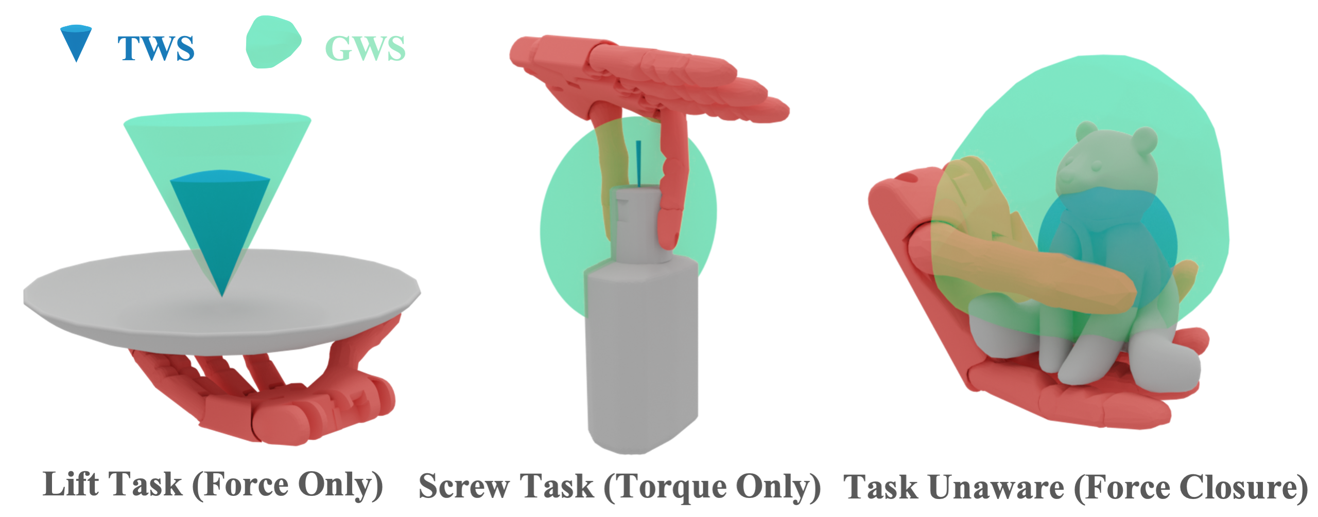
Figure 1: Task-oriented dexterous grasps synthesized by our method for different tasks. Grasp wrench space (GWS) is expected to cover each task wrench space (TWS). TWS is approximated as a 6D hyper-fan in this work.

Analytical dexterous grasp synthesis is often performed by optimizing some grasp quality metrics, so they are constrained by the deficiencies of grasp analysis, i.e. being computationally expensive or non-differentiable. Therefore, existing synthesis methods have to either perform approximations that lead to physical inaccuracies [5, 6], or resort to gradient-free methods which suffer from low grasp quality and mode collapse [7]. The key reason behind all the above problems is that most grasp metrics [3, 4, 8] are built upon the Grasp Wrench Space (GWS), which is defined as the set of wrenches that the grasp contacts can exert on the object. However, GWS is difficult to model due to its irregularity.

In this work, we propose a novel GWS boundary estimator, thus enabling the gradient-based task-oriented dexterous grasp synthesis for the first time, pushing forward the research of both analytical grasp analysis and synthesis.

Our key contribution is a fast, accurate, and differentiable GWS boundary estimator under the physically correct max-magnitude ($L_{\infty}$) bound assumption [9] for dexterous hands, i.e. each contact force is bounded to 1. Using the property of Minkowski sum, we find a simple mapping from an arbitrary 6D unit direction to a point on the GWS boundary. We can then get dense points by parallel sampling and mapping without iterative optimization. The time complexity is also linear to the contact number, making it possible for the analysis of contact-rich tasks.

Second, We propose a differentiable task-oriented energy for gradient-based grasp synthesis and a task-oriented metric for evaluation. The energy can be used in both non- and force-closure scenarios. The metric evaluates the wrench directions to measure the robustness of non-force-closure grasps. It is complementary to existing metrics that only evaluate the wrench lengths.

Finally, we improve the previous gradient-based dexterous grasp synthesis pipeline [10]. One great challenge is the non-differentiability of nearest-points calculation on object mesh from predefined hand points. It is alleviated in [10] by initialization tricks and a hybrid optimizer, but these solutions are not fundamental. We tackle it with a novel differentiable technique by perturbation and barycentric interpolation.

Through extensive experiments, we verify the efficiency and effectiveness of our methods. Our GWS boundary estimator can run in several milliseconds on GPUs with minimal memory overhead, more than three orders of magnitude faster than the traditional discretization-based method. We also synthesize 0.1 million grasps to show that our pipeline can outperform the SOTA task-unaware force-closure grasp synthesis method by a large margin. Finally, some qualitative results of task-oriented grasps are visualized.

In summary, our main contributions are (i) a fast, accurate, and differentiable $O(mK)$ algorithm ($m$ is the contact number and $K$ is the sample number) to approximate the physically correct grasp wrench boundary for dexterous hands, (ii) a task-oriented energy for gradient-based grasp synthesis, (iii) a task-oriented metric for non-force-closure grasps, and (iv) an improved dexterous grasp synthesis pipeline with better differentiability.

II Related Work

Task-unaware grasp analysis focus on the force closure property [11], which indicates whether a grasp can resist any external wrench applied to the object. To evaluate force closure, GWS is introduced, which is also the foundation of most metrics. A review for grasp quality measures can be found in [12]. To estimate the GWS, a common and efficient way is to calculate the convex hull over discretized friction cones under the sum-magnitude ($L_{1}$) bound assumption [3], i.e. all contact forces sum up to 1. But this assumption is physically incorrect for fully actuated robotic hands [9]. On the other hand, under the physically correct $L_{\infty}$ assumption, the conventional discretization-based method has exponential time complexity to the contact numbers [3]. Some works [13, 14, 4] use optimization to speed up the calculation under $L_{\infty}$ assumption, but they are non-differentiable w.r.t. hand pose. We propose the first algorithm to approximate the GWS boundary that is both efficient and physically correct, meanwhile being fully differentiable.

Task-oriented grasp analysis traditionally uses TWS to describe a task. Some works [15, 16, 17] estimate TWS from human-captured data, but the data acquisition is difficult. Others [18, 4] use Object Wrench Space as TWS when task specification is unknown. Most works approximate TWS as an ellipsoid or a ball to make it practical. Few works study non-force-closure cases [19, 20], but their settings are trivial. Our work formulates TWS as a hyper-fan and can deal with both force-closure and non-force-closure scenarios.

Dexterous grasp synthesis literature can be broadly categorized into two classes: analytical and data-driven methods. Some early reviews can be found in [21, 22]. Analytical methods optimize some analytic quality metrics, e.g. $\epsilon$ metric, to find good grasps. They often assume the object mesh is known and don’t address the perception problem. Previous methods such as GraspIt! [7] use sampling-based methods, and are inefficient for high degree of freedom (DoF) dexterous hands. [23] introduces dimensionality reduction but sacrifices the flexibility. More recent works [5, 6, 24] use gradient-based optimization with differentiable approximations of $\epsilon$ metric, but are limited to task-unaware force-closure grasps with weak physical interpretations. Another line of work [25, 26] synthesizes dexterous grasp by a differentiable simulator but its gradient may be inaccurate [27].

Data-driven methods [28, 29] use deep learning to learn from data. They often rely on analytical methods for data preparation [10, 26] and post-processing [30, 31], because collecting large-scale human data is expensive and the network prediction may be inaccurate. Recent trend of dexterous grasping uses reinforcement learning [32, 33] and imitation learning [34], but [35] shows grasp synthesis still helps.

III Preliminaries

Consider an object grasped by a hand with $m$ contacts. For each contact $i\in[1,2,\cdots,m]$, let $\mathbf{p}_{i}\in\mathbb{R}^{3}$ be the contact position, $\mathbf{n}_{i}\in\mathbb{R}^{3}$ be the inward-pointing surface unit normal, and $\mathbf{d}_{i},\mathbf{e}_{i}\in\mathbb{R}^{3}$ be two unit tangent vectors satisfying $\mathbf{n}_{i}=\mathbf{d}_{i}\times\mathbf{e}_{i}$, all of which are defined in the object coordinate frame. We use the most popular contact model, the point contact with friction (PCF) model in our paper (but our method can also work for the soft contact model):

$$\mathcal{F}_{i}=\left\{\mathbf{f}_{i}\in\mathbb{R}^{3}~{}|~{}0\leq f_{i1},f_{i2}^{2}+f_{i3}^{2}\leq\mu^{2}f_{i1}^{2}\right\}$$ (1)

$$\mathbf{G}_{i}=\begin{bmatrix}\mathbf{n}_{i}&\mathbf{d}_{i}&\mathbf{e}_{i}\\ \mathbf{p}_{i}\times\mathbf{n}_{i}&\mathbf{p}_{i}\times\mathbf{d}_{i}&\mathbf{p}_{i}\times\mathbf{e}_{i}\\ \end{bmatrix}\in\mathbb{R}^{6\times 3}$$ (2)

where $\mathcal{F}_{i}$ contains all possible forces that can be generated by contact $i$ and the matrix $\mathbf{G}_{i}$ maps the force set $\mathcal{F}_{i}$ to wrench set $\mathcal{W}_{i}=\mathbf{G}_{i}\mathcal{F}_{i}$. $\mathbf{f}_{i}=[f_{i1},f_{i2},f_{i3}]$ and $\mu$ is the friction coefficient. The resultant wrench that can be applied to the object by the robot hand is $\mathbf{w}=\sum_{i=1}^{m}{\mathbf{G}_{i}\mathbf{f}_{i}}~{}(\mathbf{f}_{i}\in\mathcal{F}_{i})$.

Grasp Wrench Space (GWS) is then defined as the spaces of all possible $\mathbf{w}$. With the $L_{1}$ or $L_{\infty}$ assumption, i.e. $\sum_{i=1}^{m}f_{i1}\leq 1$ and $\max{f_{i1}}\leq 1$, GWS is the union or Minkowski sum of each ${\mathcal{W}_{i}}$, denoted as $\mathcal{W}_{L_{1}}=\bigcup_{i=1}^{m}{\mathcal{W}_{i}}$ and $\mathcal{W}_{L_{\infty}}=\bigoplus_{i=1}^{m}{\mathcal{W}_{i}}$, respectively. In this paper, we focus on $\mathcal{W}_{L_{\infty}}$ due to its suitability to the commonly used fully-actuated dexterous hand [9]. So hereinafter we denote $\mathcal{W}_{L_{\infty}}$ by $\mathcal{W}_{g}$ for simplicity. Grasp Wrench Hull (GWH) and Grasp Wrench Boundary (GWB) are defined as the convex hull and the boundary of $\mathcal{W}_{g}$, denoted as $\mathcal{W}_{g}^{ch}$ and $\partial\mathcal{W}_{g}$, respectively.

With these notations, $\epsilon$ metric [3] and its task-oriented extension [4] can be written as

$$\epsilon=\underset{\mathbf{w}\in\partial\mathcal{W}_{g}}{\min}\|\mathbf{w}\|,~{}\epsilon_{t}=\underset{\mathbf{w}\in\partial\mathcal{W}_{g},\mathbf{t}\in\mathcal{T},\hat{\mathbf{w}}=\hat{\mathbf{t}}}{\min}\frac{\|\mathbf{w}\|}{\|\mathbf{t}\|}$$ (3)

where $\mathcal{T}$ is TWS, $\|\cdot\|$ is the L2 length norm and $\hat{\cdot}$ means length normalization.

IV Method

IV-A Grasp Wrench Boundary Estimator

Inspired by [13, 36], we propose a novel, fast, accurate, and differentiable algorithm to directly construct GWB by sampling and mapping. The key is to map an arbitrary 6D unit direction to a point on GWB. We start by defining a support mapping $s_{\mathcal{A}}$ of a nonempty compact set $\mathcal{A}\subset\mathbb{R}^{n}$:

$$s_{\mathcal{A}}(\mathbf{u})=\underset{\mathbf{a}\in\mathcal{A}}{\arg\max}~{}\mathbf{u}^{T}\mathbf{a},\|\mathbf{u}\|=1$$ (4)

This mapping returns the furthest point in $\mathcal{A}$ on the given unit direction $\mathbf{u}\in\mathbb{R}^{n}$, as shown in Fig. 2. This mapping also has three useful properties [37, 13]:

Property 1

$\forall\mathbf{u}$, $s_{\mathcal{A}}(\mathbf{u})\in\partial\mathcal{A}$. If $\mathcal{A}$ is convex, $\forall\mathbf{x}\in\partial\mathcal{A}$, $\exists\mathbf{u}$, s.t. $s_{\mathcal{A}}(\mathbf{u})=\mathbf{x}$.

Property 2

$s_{\mathcal{A\bigoplus B}}(\mathbf{u})=s_{\mathcal{A}}(\mathbf{u})+s_{\mathcal{B}}(\mathbf{u})$

Property 3

$s_{\mathbf{C}(\mathcal{A})}(\mathbf{u})=\mathbf{C}\cdot s_{\mathcal{A}}(\mathbf{C}^{T}\mathbf{u})$, where $\mathbf{C}\in\mathbb{R}^{p\times n}$ and $p$ is any positive integer.

Proof:

$s_{\mathbf{C}(\mathcal{A})}(\mathbf{u})=\underset{\mathbf{C}\mathbf{a}\in\mathbf{C}(\mathcal{A})}{\arg\max}~{}\mathbf{u}^{T}(\mathbf{C}\mathbf{a})\\ ~{}~{}~{}~{}~{}~{}~{}~{}~{}~{}~{}~{}~{}~{}~{}~{}~{}~{}~{}~{}~{}~{}~{}~{}~{}~{}~{}=\mathbf{C}\cdot\underset{\mathbf{a}\in\mathcal{A}}{\arg\max}~{}(\mathbf{C}^{T}\mathbf{u})^{T}\mathbf{a}\\ ~{}~{}~{}~{}~{}~{}~{}~{}~{}~{}~{}~{}~{}~{}~{}~{}~{}~{}~{}~{}~{}~{}~{}~{}~{}~{}~{}=\mathbf{C}\cdot s_{\mathcal{A}}(\mathbf{C}^{T}\mathbf{u})$ ∎

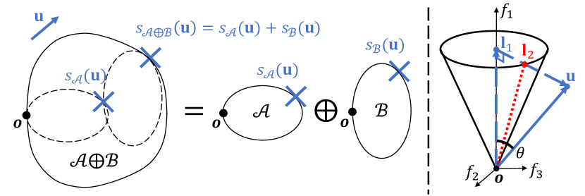
Figure 2: Left: Illustration of the support mapping $s_{\mathcal{A}}(\mathbf{u})$ and Property 2. Right: Illustration of $s_{\mathcal{F}_{i}}(\mathbf{u})$ for PCF contact model in 3D.

In our scenario, $\mathcal{F}_{i}$, $\mathcal{W}_{i}$ and $\mathcal{W}_{g}$ are all convex. So Prop. 1 indicates that if we know $s_{\mathcal{W}_{g}}$ and sample enough $\mathbf{u}$, we can get all points on $\partial\mathcal{W}_{g}$. However, since $\mathcal{W}_{g}$ is complex, it is intractable to directly get the analytical expression of $s_{\mathcal{W}_{g}}$. But we can leverage Prop. 2 and 3 to make it tractable:

$$s_{\mathcal{W}_{g}}(\mathbf{u})=s_{\bigoplus_{i=1}^{m}\mathcal{W}_{i}}(\mathbf{u})=\sum_{i=1}^{m}s_{\mathcal{W}_{i}}(\mathbf{u})=\sum_{i=1}^{m}\mathbf{G}_{i}s_{\mathcal{F}_{i}}(\mathbf{G}_{i}^{T}\mathbf{u}).$$ (5)

where $m$ is the contact number.

Now if we can get $s_{\mathcal{F}_{i}}$, we immediately know $s_{\mathcal{W}_{g}}$. For PCF contact model, $\mathcal{F}_{i}$ is a 3D cone, so the analytical expression of $s_{\mathcal{F}_{i}}$ is trivial. As shown in Fig. 2, we can use geometric intuition to directly solve:

$$s_{\mathcal{F}}(\mathbf{u})=\left\{\begin{array}[]{ll}\text{any point on the bottom},&\theta=0\\ \mathbf{l}_{2},&0<\theta<\alpha\\ \text{any point on line $\overline{\mathbf{o}\mathbf{l}_{2}}$},&\theta=\alpha\\ \mathbf{0},&\alpha<\theta<\pi\\ \end{array}\right.$$ (6)

where $\mathbf{l}_{1}$ is the projection of $\mathbf{u}$ onto $+f_{1}$ axis $\mathbf{l}_{2}$ is the intersection between the 3D cone and $\overline{\mathbf{l}_{1}\mathbf{u}}$, $\theta=\angle(\mathbf{l}_{1},\mathbf{u})$, and $\alpha=\angle(\mathbf{l}_{1},\mathbf{l}_{2})+\frac{\pi}{2}$. For the soft contact model in 4D, we can utilize Cauchy-Schwarz inequality to get similar results.

Combining Eq. 5 and 6, we get the desired mapping from an arbitrary 6D unit direction to points on GWB without any approximation. To get dense points $\{\mathbf{w}_{k}\}~{}(k=1,2,...,K)$ on $\partial\mathcal{W}_{g}$, we only need to uniformly sample $K$ ($K$ is a hyperparameter) $\mathbf{u}_{k}$ and map them by $s_{\mathbf{W}_{g}}$. This process does not need any optimization and can be fully paralleled for different contacts and samples. This approach also reduces the exponential time complexity of the classic method [3] for the contact number to linear.

Differentiability. Although the differentiability of Eq. 6 is bad, $s_{\mathcal{W}_{g}}(\mathbf{u})$ is well differentiable w.r.t. the contact position $\mathbf{p}_{i}$ and normal $\mathbf{n}_{i}$ when $s_{\mathcal{F}_{i}}(\mathbf{u})\neq\mathbf{0}$, due to the matrix $\mathbf{G}_{i}$ in Eq. 5. In practice, we detach the gradient of Eq. 6.

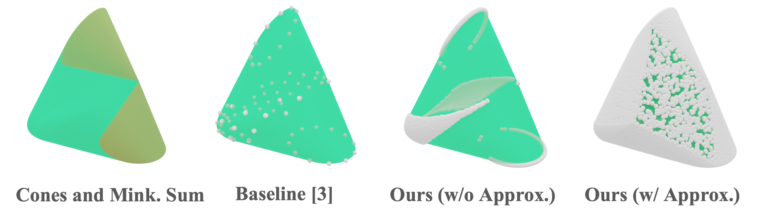
Figure 3: Points (white) sampled by different methods on GWB (green). We only visualize the 3D force space.

Approximation. $s_{\mathcal{F}}$ in Eq. 6 is not a one-to-one mapping when $\theta=0$ or $\alpha$. One simple choice is to ignore these two cases because they are almost impossible to be satisfied by the sampled direction $\mathbf{u}$. In this way, the generated points form GWH rather than GWB, as shown in Fig.3. To fill in the missing region on GWB, we propose an approximation:

$$s_{\mathcal{F}}(\mathbf{u})=\left\{\begin{array}[]{ll}\mathbf{l}_{1},&\theta=0\\ \mathbf{l}_{1}+\theta/\delta\cdot(\mathbf{l}_{2}-\mathbf{l}_{1}),&0<\theta<\delta\\ \mathbf{l}_{2},&\delta\leq\theta\leq\alpha-\delta\\ (\alpha-\theta)/\delta\cdot\mathbf{l}_{2},&\alpha-\delta<\theta<\alpha\\ \mathbf{0},&\alpha\leq\theta\leq\pi\\ \end{array}\right.$$ (7)

where $\delta$ is a hyperparameter to control the degree of approximation. The basic idea is to relax the equality conditions and interpolate on line $\overline{\mathbf{l}_{1}\mathbf{l}_{2}}$ and $\overline{\mathbf{o}\mathbf{l}_{2}}$. We don’t relax around $\mathbf{0}$, as doing so could affect sampled points near the origin and disrupt the metric accuracy. We argue that our approximation is also physically more reasonable than discretized friction cones because ours are isotropic.

Coordinate Frame Modification. Another issue we meet is the uneven distribution of sampled points on GWB. Evenly sampled $\mathbf{u}$ can lead to evenly distributed points on $\partial\mathcal{W}_{g}$ only when GWS is a sphere. The greater the deviation of GWS from a sphere, the more uneven the sampled points are. One source of such deviations is the choice of the origin and unit of the object coordinate frame. If the unit is too small, the torque space will be much smaller than the force space. To achieve frame invariance, we use the same transformation $\mathbf{p}^{\prime}_{i}=\frac{1}{d}(\mathbf{p}_{i}-\mathbf{c})$ as [13] in Eq. 2, where $\mathbf{c}=\frac{1}{m}\sum_{i=1}^{m}\mathbf{p}_{i}$ and $d=\frac{1}{m}\sum_{i=1}^{m}\|\mathbf{p}_{i}-\mathbf{c}\|_{2}$. We leave it to future work to figure out how to sample more evenly with fewer samples.

IV-B Differentiable Task-Oriented Energy

In this section, we first describe our formulation of the task wrench space, and then introduce the energy for task-oriented dexterous grasp synthesis.

We formulate the TWS as a 6-dimensional hyper-fan:

$$\mathcal{T}(\mathbf{t}_{c},\gamma)=\{\mathbf{t}\in\mathbb{R}^{6}~{}|~{}\angle(\mathbf{t},\mathbf{t}_{c})\leq\gamma,\|\mathbf{t}\|=\|\mathbf{t}_{c}\|\}$$ (8)

Although this formulation is simple, we argue that it can express a wide range of tasks, which typically fall into two categories: resisting external perturbations and applying active wrenches. For the first case, we denote the equivalent effect of the external perturbations as force $\mathbf{f}_{t}$ exerted on point $\mathbf{p_{t}}$. The second case can be represented by an active wrench $\mathbf{w}_{t}$. In summary, we decompose $\mathbf{t}_{c}$ into $[\mathbf{f}_{t},\mathbf{p}_{t}^{\prime}\times\mathbf{f}_{t}]^{T}+\mathbf{w}_{t}$ to work as an interface for users to specify tasks conveniently. Note that $\mathbf{p}_{t}^{\prime}=\frac{1}{d}(\mathbf{p}_{t}-\mathbf{c})$ as in Coordinate Frame Modification in Sec. IV-A, which makes $\mathbf{t}_{c}$ a variable when $\mathbf{f}_{t}$ and $\mathbf{p_{t}}$ are specified. Finally, the angle $\gamma\in\mathbb{R}$ is used to tolerate the potential disturbances, estimation errors, and external force fluctuations during task execution. A larger $\gamma$ demands a more robust grasp. When $\gamma=\pi$, the TWS turns into a hyper sphere, which stands for the task-unaware case. In this work, we don’t study how to get the best parameters for a task [17] and assume these parameters are given as task priors.

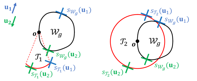
Figure 4: Illustration of our task-oriented energy for two different TWS. Unlike GWS, the dotted lines don’t belong to TWS, so $s_{\mathcal{T}_{1}}(\mathbf{u}_{1})$ is not at the origin.

Regarding the energy, we can’t directly optimize $\epsilon_{t}$ in Eq. 3. It is not differentiable when GWS doesn’t fully cover TWS (i.e. $\epsilon_{t}=0$), because $s_{\mathcal{W}_{g}}$ is not differentiable if $\mathbf{w}=\mathbf{0}$.

To encourage GWS to fully cover TWS, we get inspiration from the transportation problem of two point sets. Although finding the optimal solution by linear programming is time-consuming for a large number of points, we propose an efficient way to get a good target for each point in our scenario. As shown in Fig. 4, the target of $s_{\mathcal{W}_{g}}(\mathbf{u})$ is set to be $s_{\mathcal{T}}(\mathbf{u})$, which is easy to solve for a 6D fan. The final energy to minimize is the sum of the negative dot product:

$$E_{t}=-\sum_{k=1}^{K}\hat{s}_{\mathcal{T}}(\mathbf{u}_{k})^{T}\hat{s}_{\mathcal{W}_{g}}(\mathbf{u}_{k})$$ (9)

where $\hat{\cdot}$ is the length normalization. The target may not be optimal, but this energy works surprisingly well in practice. It increases not only the coverage rate, but also the minimum length of $\mathbf{w}$ since it encourages GWS to be the same shape as TWS. We can even use GWS of another grasp as TWS in Eq. 9, which may provide new avenues for imitation learning and worth future study.

Since $\mathbf{t}_{c}$ may be affected by $\mathbf{p}_{t}$, another regularization term $E_{r}=\|\mathbf{t}_{c}\|^{2}$ is needed to penalize its length. It can draw the contact points $\{\mathbf{p}_{i}\}$ towards the equivalent point of force application $\mathbf{p}_{t}$, in order to balance off the external perturbation. As a result, it can increase $\epsilon_{t}$ metric in Eq. 3.

IV-C Dexterous Grasp Synthesis Pipeline

In this section, we describe our dexterous grasp synthesis pipeline. Our pipeline is built upon DexGraspNet [10]. The variable to optimize is hand pose $\mathbf{q}$, including root rotation, translation, and joint angles. The input to our pipeline includes expected contact points $\{\mathbf{x}^{i}\}_{i=1}^{m}$ on hand ($m$ is the contact number), object mesh $O$ and task parameters $\{\mathbf{f}_{t},\mathbf{p}_{t},\mathbf{w}_{t},\gamma\}$. Unlike DexGraspNet, our hand points $\{\mathbf{x}^{i}\}$ do not change during optimization for simplicity. In initialization, each hand is set to face the object at a distance with zero joint angles and random jitters on the root pose.

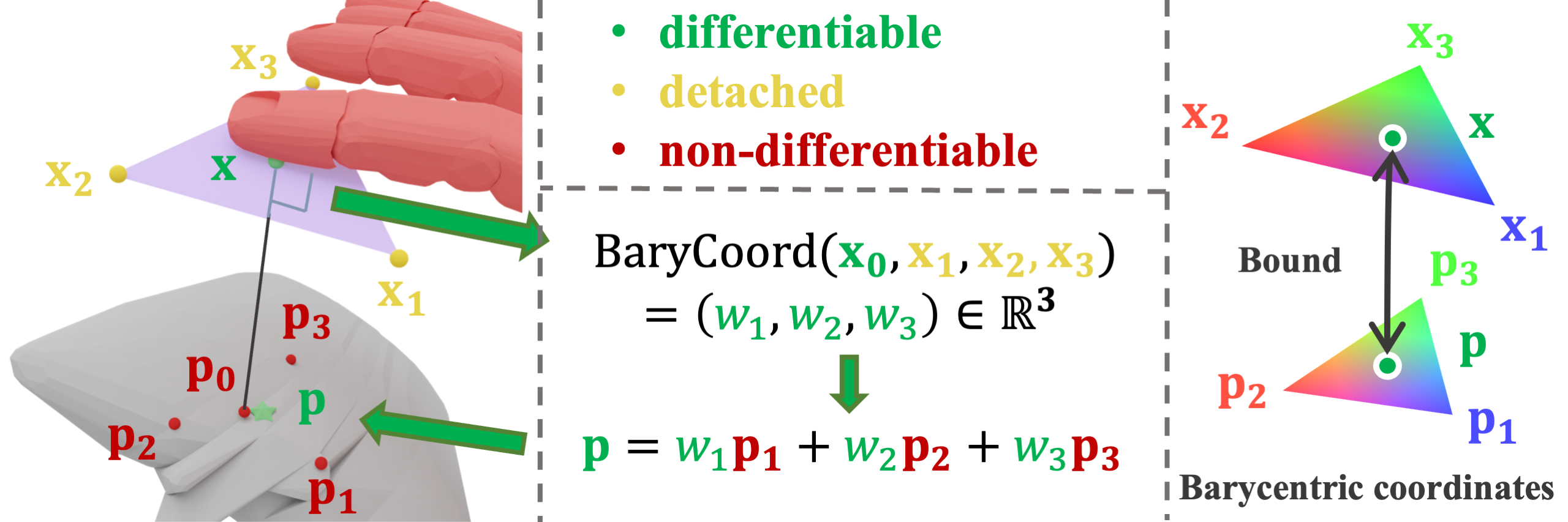
Figure 5: Differentiable method to calculate contact point $\mathbf{p}$ from hand point $\mathbf{x}$ by perturbation and Barycentric interpolation. Contact normals can be calculated in the same way.

During optimization, to calculate GWS, hand points $\{\mathbf{x}^{i}\}$ are first used to calculate the contact points $\{\mathbf{p}^{i}\}$ and normals $\{\mathbf{n}^{i}\}$, which is often achieved by finding the nearest points on the object mesh. To tackle the non-differentiability of this nearest-point calculation, we propose a novel differentiable approach to compute contact points and normals by perturbation and Barycentric interpolation. As illustrated in Fig. 5, for each hand point $\mathbf{x}$, the perturbed points are randomly sampled as a small equilateral triangle $\mathbf{x}_{j}~{}(j=1,2,3)$ centered at $\mathbf{x}$ on the tangent plane to $\overrightarrow{\mathbf{x}\mathbf{p}_{0}}$, where $\mathbf{p}_{0}$ is the nearest point of $\mathbf{x}$ on the object. Then, for each $\mathbf{x}_{j}$, we find the nearest point $\mathbf{p}_{j}$ on the object and calculate the normal $\mathbf{n}_{j}=\overrightarrow{\mathbf{x}_{j}\mathbf{p}_{j}}$. Differentiable Barycentric interpolation is finally used to calculate $\mathbf{p}$ and $\mathbf{n}$, respectively. This approach is also robust to the object surface geometry because it doesn’t use the mesh normals. With this approach, we can converge faster and better than [10] even without their initialization tricks and hybrid optimizer.

Another issue we meet is the unnatural hand pose, where the finger back is touching the object. So we add an energy $E_{n}=-\sum_{i=1}^{m}\mathbf{r}_{i}^{T}\hat{\mathbf{p}}^{h}_{i}$, where $\mathbf{r}_{i}$ is the predefined front surface normal for each hand link. $\mathbf{p}^{h}_{i}$ is contact point $\mathbf{p}^{i}$ in the local hand link coordinate frame. $\hat{\cdot}$ is the length normalization.

Finally, we remove the penetration energy in DexGraspNet [10] and instead use a simulator Isaac Gym [38] to automatically detect and fix the penetration. Specifically, at the end of each iteration, we use updated pose $\mathbf{q}$ after gradient descent as the target position to simulate one step. The new $\mathbf{q}$ from the simulation result is then used for the next iteration. It can better prevent penetration and out-of-limit joints.

In summary, the total energy consists of task energy $E_{t}$ in Eq. 9, task regularization $L_{r}$, nature energy $E_{n}$ and distance energy $E_{d}=\sum_{i=1}^{m}\|\mathbf{x}^{i}-\mathbf{p}^{i}\|^{2}$ to encourage the hand to touch the object.

IV-D Task-Oriented Metric: Max Angle

In this section, we propose a novel task-oriented metric to evaluate the wrench direction for non-force-closure grasps. Given the central wrench $\mathbf{t}_{c}$ for a task, our metric measures how much an external wrench should deviate from $\mathbf{t}_{c}$ to break the grasp. The geometry meaning is the max angle of the inscribed task hyper-fan in GWS, denoted as:

$$\gamma_{m}=\max\{\gamma~{}|~{}\hat{\mathcal{T}}(\mathbf{t}_{c},\gamma)\subset\hat{\mathcal{W}}_{g}\}$$ (10)

where $\hat{\cdot}$ means length normalization for each element in the set. In this section, we only care about the wrench direction, so all points need to be normalized in length. For simplicity, $\hat{\cdot}$ is omitted hereinafter.

Next, we introduce an efficient sampling-based algorithm to calculate $\gamma_{m}$. The basic idea is to sample many 2D planes that contain $\mathbf{t}_{c}$, and calculate the arc around $\mathbf{t}_{c}$ covered by GWS on each plane. $\gamma_{m}$ is the angle of the minimum arc opening from $\mathbf{t}_{c}$ in all 2D planes.

Specifically, we first sample many 6D unit directions $\{\mathbf{v}_{j}\}$ perpendicular to $\mathbf{t}_{c}$. For each $\mathbf{v}_{j}$, we calculate the angle $\gamma_{j}$ of arc opening from $\mathbf{t}_{c}$ covered by GWS. With enough sampling, the minimum $\gamma_{j}$ will converge to $\gamma_{m}$.

Fig. 6 shows how to solve $\gamma_{j}$ for each sampled $\mathbf{v}_{j}$. By definition, $\gamma_{j}$ is equal to the angle between $\mathbf{t}_{c}$ and the furthest point $\mathbf{w}_{j}\in\mathcal{W}_{g}$ on the arc. Although the ground truth furthest point $\mathbf{w}^{gt}_{j}$ is hard to compute, it can be approximated by the furthest point among the projection of $\mathbf{w}^{k}\in\partial\mathcal{W}_{g}$ on the arc, where $\mathbf{w}^{k}$ is sampled by our GWB estimator. The projection on an arc can be achieved by two steps: first project $\mathbf{w}^{k}$ onto the 2D plane formed by $\mathbf{t}_{c}$ and $\mathbf{v}_{j}$, and then normalize the length to get $\mathbf{w}^{k}_{j}$. Finally, $\gamma_{j}\approx\max_{k=1,2,...,K}\gamma_{j}^{k}$, where $\gamma_{j}^{k}=\angle(\mathbf{t}_{c},\mathbf{w}^{k}_{j})$.

One problem is that ground truth $\gamma_{j}^{gt}$ can be very different from $\max_{k}\gamma_{j}^{k}$, because the distance between $\mathbf{w}^{gt}_{j}$ and $\mathbf{w}^{k}_{j}$ can be large. However, since $\gamma_{j}^{gt}$ is always lower than estimated $\gamma_{j}$ (assuming $\{\mathbf{w}^{k}\}$ are uniform to some extent), in theory the final metric $\gamma_{m}=\min_{j}\gamma_{j}$ will converge to the correct value with enough sampling of $\mathbf{v}_{j}$. To improve sampling efficiency and accelerate convergence, we optimize $\gamma_{m}$ by a genetic-style algorithm. In each iteration, we increase the sampling weights near those $\mathbf{v}_{j}$ with small $\gamma_{j}$.

The only remaining problem is to judge whether the direction of $\mathbf{t}_{c}$ is covered by GWS. We tackle it by randomly sampling many 6-subsets of $\{\mathbf{w}^{k}\}$ as simplices and seeing whether $\mathbf{t}_{c}$ can be expressed as non-negative linear combinations of vertices of a simplex. This method can also be used to check force closure. A GWS satisfies force closure if any unit 6D directions $\pm\mathbf{a}$ are both contained. This is more accurate than simply judging whether exists a $\mathbf{w}^{k}=\mathbf{0}$, due to the uneven sampling.

Fig. 6 shows the estimated max angle for the plate lifting in Fig. 1. Our genetic-style algorithm is more accurate than naive uniform sampling with the same total sampling number of $\mathbf{v}_{j}$. The time cost is less than 40ms on a 3090 GPU.

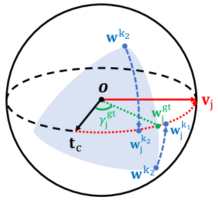
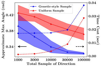
Figure 6: Left: Illustration of calculating max angle $\gamma_{m}$. All points are on a 6D unit sphere. The light blue area represents all directions covered by $\mathcal{W}_{g}$. Right: convergence curve of $\gamma_{m}$ for lift task in Fig. 1.

V Experiments

V-A Experiments on Grasp Wrench Boundary Estimation

Here we evaluate the efficiency of our GWB estimator.

Experiment setup: For each parameter setting, we randomly sample $m$ contact points on 49 objects from YCB dataset [39], and use them to calculate GWS. We also change friction coefficient $\mu$ in $[0.2,0.3,0.5,1.0]$, resulting in $49\times 4=196$ data per experiment. All metrics below are averaged over these 196 data.

We evaluate the accuracy, density and speed by three metrics: 1) average relative length error (RLE) (unit: $10^{-2}$) of sampled points $\mathbf{w}$ to the ground truth boundary in the direction of $\mathbf{w}$. The error of each point is $\max_{q\mathbf{w}\in\partial\mathcal{W}_{g}^{gt}}\frac{q-1}{q}$, which can be viewed as a Second-order Cone Program (SOCP) and solved by [40]. 2) Sparsity (SP) (unit: rad), the expectation of the min angle between sampled points $\mathbf{w}$ and uniformly distributed points on the 6D sphere. Since this metric requires GWS to fully cover the sphere, we filter out non-force-closure data by the force-closure checking method in Sec. IV-D, and resample data. 3) time (t) (unit: ms).

TABLE I: Comparison of Our GWS Estimator with Baseline.

	5 Contacts				7 Contacts
	Baseline			Ours	Baseline			Ours
	4	6	8		4	6	8
RLE$\downarrow$	5.30	2.36	1.26	0.43	6.49	2.78	-	0.70
SP $\downarrow$	0.48	0.42	0.38	0.29	0.36	0.31	-	0.26
t $\downarrow$	4e3	2e4	4e4	20	5e4	2e5	2e6	20

Result comparison with the baseline. We use the classic discretization-based method [3] under $L_{\infty}$ assumption as the baseline and change the discretization number $d=4,6,8$. Our method has two parameters: angle $\delta$ for approximation and sample number $K$. We set $\delta=15^{\circ}$ and $K=1e6$ as our default value. Table I shows that our method is significantly faster than the baseline, because we can parallel on GPU but their QuickHull algorithm (Pyhull package) has to iterate on CPU. When the contact number $m$ increases, our time increases linearly but theirs increases exponentially. We don’t run $m=7,d=8$ for all 196 data since the speed is so slow that the other two metrics are meaningless. Our memory cost is also low (about several MiB). Besides, ours are denser and more accurate than the baseline, since they only use a few points on each friction cone but we can map to any point.

TABLE II: Hyperparameter Analysis of Our Method with 5 Contacts.

	$\delta$ (with $K=1e5$)				K (with $\delta=15^{\circ}$)
	0∘	15∘	30∘	45∘	1e3	1e4	1e5	1e6
RLE$\downarrow$	0.00	0.42	5.45	19.4	0.43	0.42	0.42	0.43
SP $\downarrow$	0.44	0.36	0.36	0.36	0.55	0.45	0.36	0.29
t $\downarrow$	3.2	3.2	3.2	3.2	1.7	1.9	3.2	19.4

Hyperparameter analysis. In Tab. II, we investigate the effect of $\delta$ and $K$. For $\delta=0^{\circ}$, there is no approximation at all, but the samples are unevenly distributed. $\delta=15^{\circ}$ is a good choice to balance accuracy and uniformity. Increasing $K$ can improve the density, but the time cost increases. How to sample more uniformly with small $K$ worth future study.

V-B Task-Unaware Force-Closure Dexterous Grasp Synthesis

To validate the effectiveness of our dexterous grasp synthesis pipeline, we compare our method with the state-of-the-art analytical method DexGraspNet [10] for force-closure grasps synthesis. [7, 25, 26] is not compared due to the slow running speed or its close source.

Experiment setup: We use the same large-scale object assets in DexGraspNet with more than 5700 objects. 20 grasps are synthesized for each object, resulting in more than 0.1 million grasps in total. We use the default setting of DexGraspNet as the baseline. For our method, we set $m=5,\delta=15^{\circ},K=10^{4}$ to balance the speed and the performance. Five hand contact points are assigned as the center points on the front surface of each distal finger link. This is a simple and flexible way to use all fingers. We optimize 600 iterations with naive gradient descent.

Evaluation metrics are similar to DexGraspNet: 1) Simulation success rate (SS), the ratio of synthesized grasps that can remain stationary under external forces in six directions in Isaac Gym [38]. 2) Max penetration depth (MP) of each grasp. 3) $\epsilon$ metric computed by our GWB estimator. If the distance between a hand link and the object is larger than 5$mm$, this link is not in contact. Contact points are chosen as the nearest points to the object on each hand link in contact.

As shown in Tab. III, our method can outperform DexGraspNet in all metrics. Thanks to the good gradient from our novel energy in Sec. IV-B and the differentiable approach in Sec. IV-C, we can converge better with fewer iterations (600 vs 6000). We also use fewer tricks in initialization and optimizer. Using Isaac Gym to check and fix collisions reduces penetration, but we meet unknown issues in the low level of Isaac Gym if paralleling many objects. Although we can synthesize a single grasp faster, we are slower than DexGraspNet to generate all grasps (150 vs 60 GPU hours). The parallelism of our algorithm is expected to be greatly improved by a better simulator.

TABLE III: 0.1 Million Force-closure Dexterous Grasp Synthesis

	SS ($\%$) $\uparrow$	MP ($mm$) $\downarrow$	$\epsilon\uparrow$
DexGraspNet	37.0	5.4	0.77
Ours	57.1	2.4	0.93

V-C Task-Oriented Dexterous Grasp Synthesis

Since we are the first work to tackle the task-oriented dexterous grasp synthesis, there is no large benchmark for comparison. We keep most experiment settings the same as in V-B and manually assign the TWS and hand contact points for each task. To screw the knob, major task wrench $\mathbf{t}_{c}=[0,0,0,\pm 1,0,0]^{T}$ and task angle $\gamma=\pi/8$, indicating the in-plane rotation. The hand contact points are selected as the center of the distal link on the thumb and index finger. To turn the handle, $\mathbf{t}_{c}=[0,0,-1,0,0,0]^{T}$, $\gamma=\pi/8$ or $\pi$, indicating non-force-closure and force-closure. The hand contact points are selected as the center of the distal link on the thumb and the middle link on the other four fingers.

Some qualitative results are shown in Fig. 1 and Fig. 7. Our method can generate diverse grasps for different tasks. Although the third grasps of each group are not human-like, they are still valid grasps that can execute the desired task. How to improve it deserves future study.

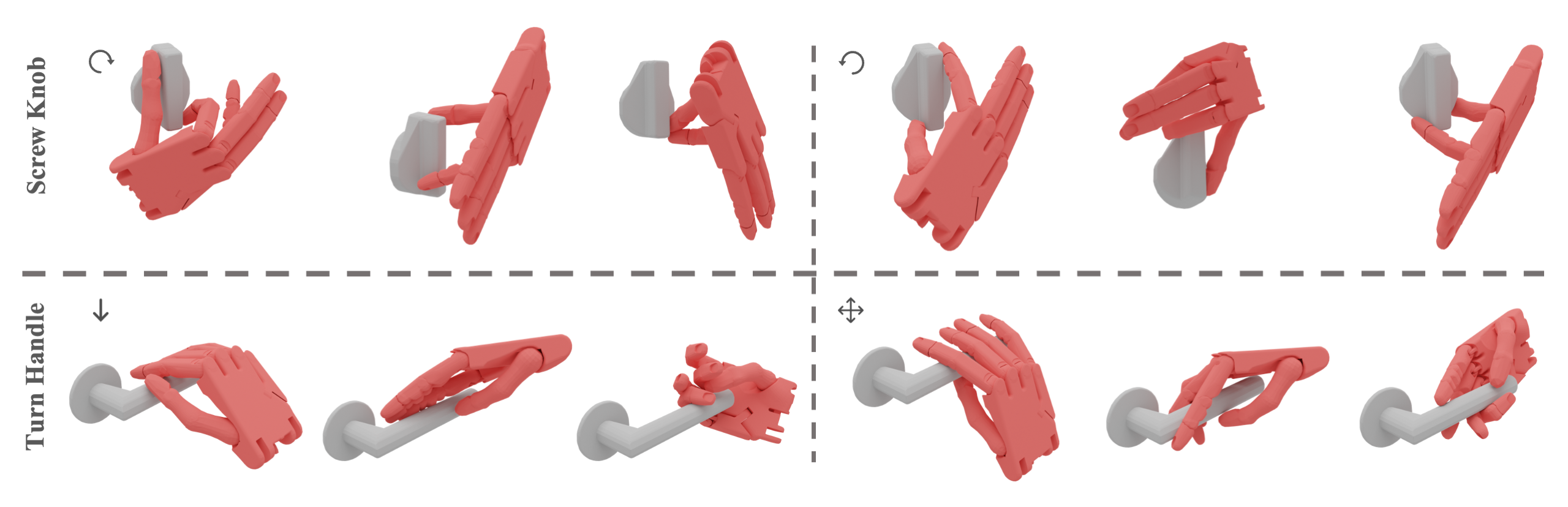
Figure 7: Visualization of synthesized task-oriented grasps. Three grasps are shown for each task, denoted by the upper left arrow. The fourth task means force closure. Each third grasp is an unnatural example.

VI Limitations and Conclusions

In this paper, we propose the first analytical gradient-based optimization algorithm for task-oriented dexterous grasp synthesis. Our key contribution is a novel, fast, accurate, and differentiable grasp wrench boundary estimator. Our grasp wrench boundary also has a good physical interpretation for dexterous hands. Based on it, we propose a task-oriented energy for gradient-based optimization and a task-oriented metric for evaluation. We also improve the differentiability of the previous dexterous grasp synthesis pipeline. Extensive experiments verify the efficiency and effectiveness of our novel GWB estimator and improved synthesis pipeline.

There are also limitations in this work: the gradient-based optimization is hard to jump out of local minima, the sampling on GWS is not uniform enough, the hand contact points need manually assigned, and so on. Nevertheless, we believe that our novel GWB estimator opens new room for research. We hope our work can facilitate the study of robust and flexible dexterous grasping and manipulation.

References

- [1] D. G. Kirkpatrick, B. Mishra, and C.-K. Yap, “Quantitative steinitz’s theorems with applications to multifingered grasping,” in Proceedings of the twenty-second annual ACM Symposium on Theory of Computing, 1990, pp. 341–351.
- [2] D. Kappler, J. Bohg, and S. Schaal, “Leveraging big data for grasp planning,” in 2015 IEEE international conference on robotics and automation (ICRA). IEEE, 2015, pp. 4304–4311.
- [3] C. Ferrari, J. F. Canny, et al., “Planning optimal grasps.” in ICRA, vol. 3, no. 4, 1992, p. 6.
- [4] C. Borst, M. Fischer, and G. Hirzinger, “Grasp planning: How to choose a suitable task wrench space,” in IEEE International Conference on Robotics and Automation, 2004. Proceedings. ICRA’04. 2004, vol. 1. IEEE, 2004, pp. 319–325.
- [5] T. Liu, Z. Liu, Z. Jiao, Y. Zhu, and S.-C. Zhu, “Synthesizing diverse and physically stable grasps with arbitrary hand structures using differentiable force closure estimator,” IEEE Robotics and Automation Letters, vol. 7, no. 1, pp. 470–477, 2021.
- [6] A. H. Li, P. Culbertson, J. W. Burdick, and A. D. Ames, “Frogger: Fast robust grasp generation via the min-weight metric,” arXiv preprint arXiv:2302.13687, 2023.
- [7] A. T. Miller and P. K. Allen, “Graspit! a versatile simulator for robotic grasping,” IEEE Robotics & Automation Magazine, vol. 11, no. 4, pp. 110–122, 2004.
- [8] M. Liu, Z. Pan, K. Xu, K. Ganguly, and D. Manocha, “Deep differentiable grasp planner for high-dof grippers,” arXiv preprint arXiv:2002.01530, 2020.
- [9] R. Krug, Y. Bekiroglu, and M. A. Roa, “Grasp quality evaluation done right: How assumed contact force bounds affect wrench-based quality metrics,” in 2017 IEEE International Conference on Robotics and Automation (ICRA). IEEE, 2017, pp. 1595–1600.
- [10] R. Wang, J. Zhang, J. Chen, Y. Xu, P. Li, T. Liu, and H. Wang, “Dexgraspnet: A large-scale robotic dexterous grasp dataset for general objects based on simulation,” in 2023 IEEE International Conference on Robotics and Automation (ICRA). IEEE, 2023, pp. 11 359–11 366.
- [11] K. Lakshminarayana, “Mechanics of form closure,” ASME report, 1978.
- [12] M. A. Roa and R. Suárez, “Grasp quality measures: review and performance,” Autonomous robots, vol. 38, pp. 65–88, 2015.
- [13] Y. Zheng and W.-H. Qian, “Improving grasp quality evaluation,” Robotics and Autonomous Systems, vol. 57, no. 6-7, pp. 665–673, 2009.
- [14] Y. Zheng, “An efficient algorithm for a grasp quality measure,” IEEE Transactions on Robotics, vol. 29, no. 2, pp. 579–585, 2012.
- [15] Z. Li and S. S. Sastry, “Task-oriented optimal grasping by multifingered robot hands,” IEEE Journal on Robotics and Automation, vol. 4, no. 1, pp. 32–44, 1988.
- [16] S. El-Khoury, R. De Souza, and A. Billard, “On computing task-oriented grasps,” Robotics and Autonomous Systems, vol. 66, pp. 145–158, 2015.
- [17] Y. Lin and Y. Sun, “Grasp planning to maximize task coverage,” The International Journal of Robotics Research, vol. 34, no. 9, pp. 1195–1210, 2015.
- [18] S. Liu and S. Carpin, “A fast algorithm for grasp quality evaluation using the object wrench space,” in 2015 IEEE International Conference on Automation Science and Engineering (CASE). IEEE, 2015, pp. 558–563.
- [19] H. Kruger and A. F. van der Stappen, “Partial closure grasps: Metrics and computation,” in 2011 IEEE International Conference on Robotics and Automation. IEEE, 2011, pp. 5024–5030.
- [20] H. Kruger, E. Rimon, and A. F. van der Stappen, “Local force closure,” in 2012 IEEE International Conference on Robotics and Automation. IEEE, 2012, pp. 4176–4182.
- [21] A. Sahbani, S. El-Khoury, and P. Bidaud, “An overview of 3d object grasp synthesis algorithms,” Robotics and Autonomous Systems, vol. 60, no. 3, pp. 326–336, 2012.
- [22] J. Bohg, A. Morales, T. Asfour, and D. Kragic, “Data-driven grasp synthesis—a survey,” IEEE Transactions on robotics, vol. 30, no. 2, pp. 289–309, 2013.
- [23] M. T. Ciocarlie and P. K. Allen, “Hand posture subspaces for dexterous robotic grasping,” The International Journal of Robotics Research, vol. 28, no. 7, pp. 851–867, 2009.
- [24] H. Dai, A. Majumdar, and R. Tedrake, “Synthesis and optimization of force closure grasps via sequential semidefinite programming,” Robotics Research: Volume 1, pp. 285–305, 2018.
- [25] D. Turpin, L. Wang, E. Heiden, Y.-C. Chen, M. Macklin, S. Tsogkas, S. Dickinson, and A. Garg, “Grasp’d: Differentiable contact-rich grasp synthesis for multi-fingered hands,” in European Conference on Computer Vision. Springer, 2022, pp. 201–221.
- [26] D. Turpin, T. Zhong, S. Zhang, G. Zhu, J. Liu, R. Singh, E. Heiden, M. Macklin, S. Tsogkas, S. Dickinson, et al., “Fast-grasp’d: Dexterous multi-finger grasp generation through differentiable simulation,” arXiv preprint arXiv:2306.08132, 2023.
- [27] Y. D. Zhong, J. Han, and G. O. Brikis, “Differentiable physics simulations with contacts: Do they have correct gradients wrt position, velocity and control?” arXiv preprint arXiv:2207.05060, 2022.
- [28] L. Shao, F. Ferreira, M. Jorda, V. Nambiar, J. Luo, E. Solowjow, J. A. Ojea, O. Khatib, and J. Bohg, “Unigrasp: Learning a unified model to grasp with multifingered robotic hands,” IEEE Robotics and Automation Letters, vol. 5, no. 2, pp. 2286–2293, 2020.
- [29] W. Wei, D. Li, P. Wang, Y. Li, W. Li, Y. Luo, and J. Zhong, “Dvgg: Deep variational grasp generation for dextrous manipulation,” IEEE Robotics and Automation Letters, vol. 7, no. 2, pp. 1659–1666, 2022.
- [30] H. Jiang, S. Liu, J. Wang, and X. Wang, “Hand-object contact consistency reasoning for human grasps generation,” in Proceedings of the IEEE/CVF International Conference on Computer Vision, 2021, pp. 11 107–11 116.
- [31] P. Li, T. Liu, Y. Li, Y. Geng, Y. Zhu, Y. Yang, and S. Huang, “Gendexgrasp: Generalizable dexterous grasping,” in 2023 IEEE International Conference on Robotics and Automation (ICRA). IEEE, 2023, pp. 8068–8074.
- [32] P. Mandikal and K. Grauman, “Dexvip: Learning dexterous grasping with human hand pose priors from video,” in Conference on Robot Learning. PMLR, 2022, pp. 651–661.
- [33] W. Wan, H. Geng, Y. Liu, Z. Shan, Y. Yang, L. Yi, and H. Wang, “Unidexgrasp++: Improving dexterous grasping policy learning via geometry-aware curriculum and iterative generalist-specialist learning,” arXiv preprint arXiv:2304.00464, 2023.
- [34] Y. Qin, Y.-H. Wu, S. Liu, H. Jiang, R. Yang, Y. Fu, and X. Wang, “Dexmv: Imitation learning for dexterous manipulation from human videos,” in European Conference on Computer Vision. Springer, 2022, pp. 570–587.
- [35] Y. Xu, W. Wan, J. Zhang, H. Liu, Z. Shan, H. Shen, R. Wang, H. Geng, Y. Weng, J. Chen, et al., “Unidexgrasp: Universal robotic dexterous grasping via learning diverse proposal generation and goal-conditioned policy,” in Proceedings of the IEEE/CVF Conference on Computer Vision and Pattern Recognition, 2023, pp. 4737–4746.
- [36] S. Qiu and M. R. Kermani, “A new approach for grasp quality calculation using continuous boundary formulation of grasp wrench space,” Mechanism and Machine Theory, vol. 168, p. 104524, 2022.
- [37] S. R. Lay, Convex sets and their applications. Courier Corporation, 2007.
- [38] V. Makoviychuk, L. Wawrzyniak, Y. Guo, M. Lu, K. Storey, M. Macklin, D. Hoeller, N. Rudin, A. Allshire, A. Handa, et al., “Isaac gym: High performance gpu-based physics simulation for robot learning,” arXiv preprint arXiv:2108.10470, 2021.
- [39] Y. Xiang, T. Schmidt, V. Narayanan, and D. Fox, “Posecnn: A convolutional neural network for 6d object pose estimation in cluttered scenes,” arXiv preprint arXiv:1711.00199, 2017.
- [40] A. Domahidi, E. Chu, and S. Boyd, “ECOS: An SOCP solver for embedded systems,” in European Control Conference (ECC), 2013, pp. 3071–3076.