University of Science and Technology of China, Hefei, Anhui, China,
11email: lwj1217@mail.ustc.edu.cn
Solving Low-Dose CT Reconstruction via GAN with Local Coherence
Abstract
The Computed Tomography (CT) for diagnosis of lesions in human internal organs is one of the most fundamental topics in medical imaging. Low-dose CT, which offers reduced radiation exposure, is preferred over standard-dose CT, and therefore its reconstruction approaches have been extensively studied. However, current low-dose CT reconstruction techniques mainly rely on model-based methods or deep-learning-based techniques, which often ignore the coherence and smoothness for sequential CT slices. To address this issue, we propose a novel approach using generative adversarial networks (GANs) with enhanced local coherence. The proposed method can capture the local coherence of adjacent images by optical flow, which yields significant improvements in the precision and stability of the constructed images. We evaluate our proposed method on real datasets and the experimental results suggest that it can outperform existing state-of-the-art reconstruction approaches significantly.
Keywords:
CT reconstruction Low-dose Generative adversarial networks Local coherence Optical flow1 Introduction
Computed Tomography (CT) is one of the most widely used technologies in medical imaging, which can assist doctors for diagnosing the lesions in human internal organs. Due to harmful radiation exposure of standard-dose CT, the low dose CT is more preferable in clinical application [5, 7, 35]. However, when the dose is low together with the issues like sparse-view or limited angles, it becomes quite challenging to reconstruct high-quality CT images. The high-quality CT images are important to improve the performance of diagnosis in clinic [28]. In mathematics, we model the CT imaging as the following procedure
| (1) |
where denotes the unknown ground-truth picture, denotes the received measurement, and is the noise. The function represents the forward operator that is analogous to the Radon transform, which is widely used in medical imaging [24, 29]. The problem of CT reconstruction is to recover from the received .
Solving the inverse problem of (1) is often very challenging if there is no any additional information. If the forward operator is well-posed and is neglectable, we know that an approximate can be easily obtained by directly computing . However, is often ill-posed, which means the inverse function does not exist and the inverse problem of (1) may have multiple solutions. Moreover, when the CT imaging is low-dose, the filter backward projection (FBP) [12] can produce serious detrimental artifact. Therefore, most of existing approaches usually incorporate some prior knowledge during the reconstruction [15, 18, 27]. For example, a commonly used method is based on regularization:
| (2) |
where denotes the -norm and denotes the penalty item from some prior knowledge.
In the past years, a number of methods have been proposed for designing the regularization . The traditional model-based algorithms, e.g., the ones using total variation [4, 27], usually apply the sparse gradient assumptions and run an iterative algorithm to learn the regularizers [13, 19, 25, 30]. Another popular line for learning the regularizers comes from deep learning [14, 18]; the advantage of the deep learning methods is that they can achieve an end-to-end recovery of the true image from the measurement [1, 22]. Recent researches reveal that convolutional neural networks (CNNs) are quite effective for image denoising, e.g., the CNN based algorithms [11, 35] can directly learn the reconstructed mapping from initial measurement reconstructions (e.g., FBP) to the ground-truth images. The dual-domain network that combines the sinograms with reconstructed low-dose CT images was also proposed to enhance the generalizability [16, 31].
A major drawback of the aforementioned reconstruction methods is that they deal with the input CT 2D slices independently (note that the goal of CT reconstruction is to build the 3D model of the organ). Namely, the neighborhood correlations among the 2D slices are often ignored, which may affect the reconstruction performance in practice. In the field of computer vision, “optical flow” is a common technique for tracking the motion of object between consecutive frames, which has been applied to many different tasks like video generation [36], prediction of next frames [23] and super resolution synthesis [6, 32]. To estimate the optical flow field, exsting approaches include the traditional brightness gradient methods [3] and the deep networks [8]. The idea of optical flow has also been used for tracking the organs movement in medical imaging [17, 21, 34]. However, to the best of our knowledge, there is no work considering GANs with using optical flow to capture neighbor slices coherence for low dose 3D CT reconstruction.
In this paper, we propose a novel optical flow based generative adversarial network for 3D CT reconstruction. Our intuition is as follows. When a patient is located in a CT equipment, a set of consecutive cross-sectional images are generated. If the vertical axial sampling space of transverse planes is small, the corresponding CT slices should be highly similar. So we apply optical flow, though there exist several technical issues waiting to solve for the design and implementation, to capture the local coherence of adjacent CT images for reducing the artifacts in low-dose CT reconstruction. Our contributions are summarized below:
-
1.
We introduce the “local coherence” by characterizing the correlation of consecutive CT images, which plays a key role for suppressing the artifacts.
-
2.
Together with the local coherence, our proposed generative adversarial networks (GANs) can yield significant improvement for texture quality and stability of the reconstructed images.
-
3.
To illustrate the efficiency of our proposed approach, we conduct rigorous experiments on several real clinical datasets; the experimental results reveal the advantages of our approach over several state-of-the-art CT reconstruction methods.
2 Preliminaries
In this section, we briefly review the framework of the ordinary generative adversarial network, and also introduce the local coherence of CT slices.
2.0.1 Generative adversarial network.
Traditional generative adversarial network [9] consists of two main modules, a generator and a discriminator. The generator is a mapping from a latent-space Gaussian distribution to the synthetic sample distribution , which is expected to be close to the real sample distribution . On the other hand, the discriminator aims to maximize the distance between the distributions and . The game between the generator and discriminator actually is an adversarial process, where the overall optimization objective follows a min-max principle:
| (3) |
2.0.2 Local coherence.
As mentioned in Section 1, optical flow can capture the temporal coherence of object movements, which plays a crucial role in many video-related tasks. More specifically, the optical flow refers to the instantaneous velocity of pixels of moving objects on consecutive frames over a short period of time [3]. The main idea relies on the practical assumptions that the brightness of the object more likely remains stable across consecutive frames, and the brightness of the pixels in a local region are usually changed consistently [10]. Based on these assumptions, the brightness of optical flow can be described by the following equation:
| (4) |
where represents the optical flow of the position in the image. denotes spatial gradients of image brightness, and denotes the temporal partial derivative of the corresponding region.
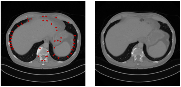
Following the equation (4), we consider the question that whether the optical flow idea can be applied to 3D CT reconstruction. In practice, the brightness of adjacent CT images often has very tiny difference, due to the inherent continuity and structural integrity of human body. Therefore, we introduce the “local coherence” that indicates the correlation between adjacent images of a tissue. Namely, adjacent CT images often exhibit significant similarities within a certain local range along the vertical axis of the human body. Due to the local coherence, the noticeable variations observed in CT slices within the local range often occur at the edges of organs. We can substitute the temporal partial derivative by the vertical axial partial derivative in the equation (4), where “z” indicates the index of the vertical axis. As illustrated in Figures 1, the local coherence can be captured by the optical flow between adjacent CT slices.
3 GANs with local coherence
In this section, we introduce our low-dose CT image generation framework with local coherence in detail.
3.0.1 The framework of our network.
The proposed framework comprises three components, including a generator , a discriminator and an optical flow estimator . The generator is the core component, and the flow estimator provides auxiliary warping images for the generation process.
Suppose we have a sequence of measurements ; for each , , we want to reconstruct its ground truth image as the equation (1). Before performing the reconstruction in the generator , we apply some prior knowledge in physics and run filter backward projection on the measurement in equation (1) to obtain an initial recovery solution . Usually contains significant noise comparing with the ground truth . Then the network has two input components, i.e., the initial backward projected image that serves as an approximation of the ground truth , and a set of neighbor CT slices 111If , ; if , . for preserving the local coherence. The overall structure of our framework is shown in Figure 2. Below, we introduce the three key parts of our framework separately.
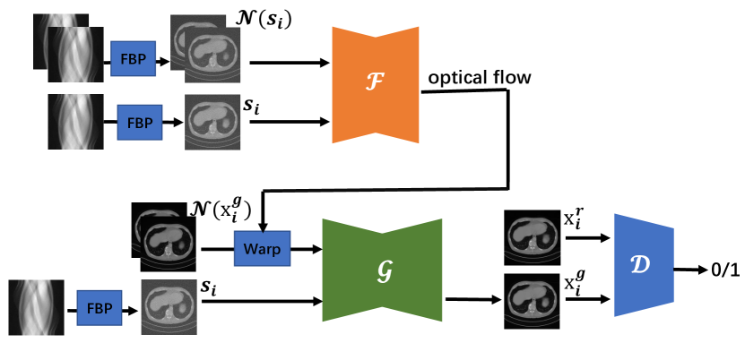
3.0.2 Optical flow estimator.
The optical flow denotes the brightness changes of pixels from to , where it captures their local coherence. The estimator is derived by the network architecture of FlowNet [8]. The FlowNet is an autoencoder architecture with extraction of features of two input frames to learn the corresponding flow, which is consist of (de)convolutional layers for both encoder and decoder.
3.0.3 Discriminator.
The discriminator assigns the label “” to real standard-dose CT images and “” to generated images. The goal of is to maximize the separation between the distributions of real images and generated images:
| (5) |
where is the image generated by (the formal definition for will be introduced below). The discriminator includes 3 residual blocks, with 4 convolutional layers in each residual block.
3.0.4 Generator.
We use the generator to reconstruct the high-quality CT image for the ground truth from the low-dose image . The generated image is obtained by
| (6) | ||||
where is the warping operator. Before generating , is reconstructed from by the generator without considering local coherence. Subsequently, according to the optical flow , we warp the reconstructed images to align with the current slice by adjusting the brightness values. The warping operator utilizes bi-linear interpolation to obtain , which enables the model to capture subtle variations in the tissue from the generated ; also, the warping operator can reduce the influence of artifacts for the reconstruction. Finally, is generated by combining and . Since is our target for reconstruction in the -th batch, we consider the difference between and in the loss. Our generator is mainly based on the network architecture of Unet [26]. Partly inspired by the loss in [2], the optimization objective of the generator comprises three items with the coefficients :
| (7) |
In (7), “” is the loss measuring the pixel-wise mean square error of the generated image with respect to the ground-truth . “” represents the adversarial loss of the discriminator , which is designed to minimize the distance between the generated standard-dose CT image distribution and the real standard-dose CT image distribution . “” denotes the perceptual loss, which quantifies the dissimilarity between the feature maps of and ; the feature maps denote the feature representation extracted from the hidden layers in the discriminator (suppose there are hidden layers):
| (8) |
where refers to the feature extraction performed on the -th hidden layer. Through capturing the high frequency differences in CT images, can enhance the sharpness for edges and increase the contrast for the reconstructed images. and are designed to recover global structure, and is utilized to incorporate additional texture details into the reconstruction process.
4 Experiment
4.0.1 Datasets.
First, our proposed approaches are evaluated on the “Mayo-Clinic low-dose CT Grand Challenge” (Mayo-Clinic) dataset of lung CT images [20]. The dataset contains 2250 two dimensional slices from 9 patients for training, and the remaining 128 slices from 1 patient are reserved for testing. The low-dose measurements are simulated by parallel-beam X-ray with 200 (or 150) uniform views, i.e., , and 400 (or 300) detectors, i.e., . In order to further verify the denoising ability of our approaches, we add the Gaussian noise with standard deviation to the sinograms after X-ray projection in 50% of the experiments. To evaluate the generalization of our model, we also consider another dataset RIDER with non-small cell lung cancer under two CT scans [37] for testing. We randomly select 4 patients with 1827 slices from the dataset. The simulation process is identical to that of Mayo-Clinic. The proposed networks were implemented in the MindSpore framework and trained on Nvidia 3090 GPU with 100 epochs.
4.0.2 Baselines and evaluation metrics.
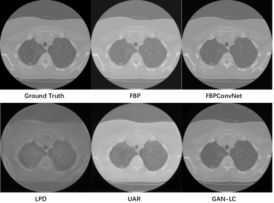
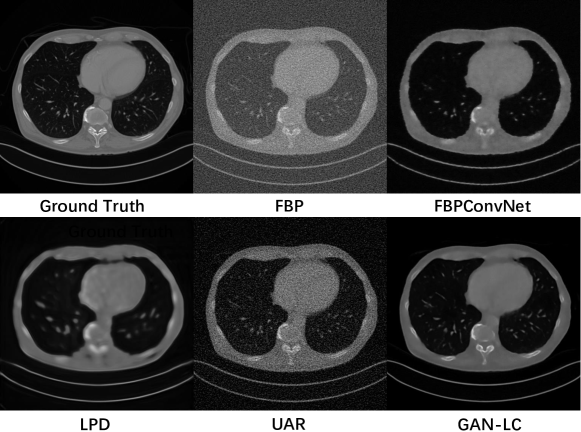
We consider several existing popular algorithms for comparison. (1) FBP [12]: the classical filter backward projection on low-dose sinograms. (2) FBPConvNet [11]: a direct inversion network followed by the CNN after initial FBP reconstruction. (3) LPD [1]: a deep learning method based on proximal primal-dual optimization. (4) UAR [22]: an end-to-end reconstruction method based on learning unrolled reconstruction operators and adversarial regularizers. Our proposed method is denoted by GAN-LC. We set for the optimization objective in equation (7) during our training process. Following most of the previous articles on 3D CT reconstruction, we evaluate the experimental performance by two metrics: the peak signal-to-noise ratio (PSNR) and the structural similarity index (SSIM) [33]. PSNR measures the pixel differences of two images, which is negatively correlated with mean square error. SSIM measures the structure similarity between two images, which is related to the variances of the input images. For both two meansures, the higher the better.
4.0.3 Results.
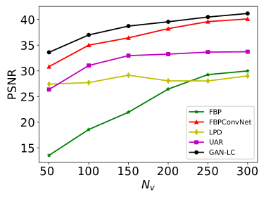
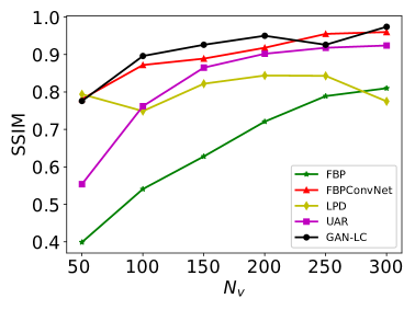
Table 1 presents the results on the Mayo-Clinic dataset, where the first row represents different parameter settings (i.e., the number of uniform views , the number of detectors and the standard deviation of Gaussian noise ) for simulating low-dose sinograms. Our proposed approach GAN-LC consistently outperforms the baselines under almost all the low-dose parameter settings. The methods FBP and UAR are very sensitive to noise; the performance of LPD is relatively stable but with low reconstruction accuracy. FBPConvNet has a similar increasing trend with our approach across different settings but has worse reconstruction quality. To evaluate the stability and generalization of our model and the baselines trained on Mayo-Clinic dataset, we also test them on the RIDER dataset. The results are shown in Table 2. Due to the bias in the datasets collected from different facilities, the performances of all the models are declined to some extents. But our proposed approach still outperforms the other models for most testing cases.
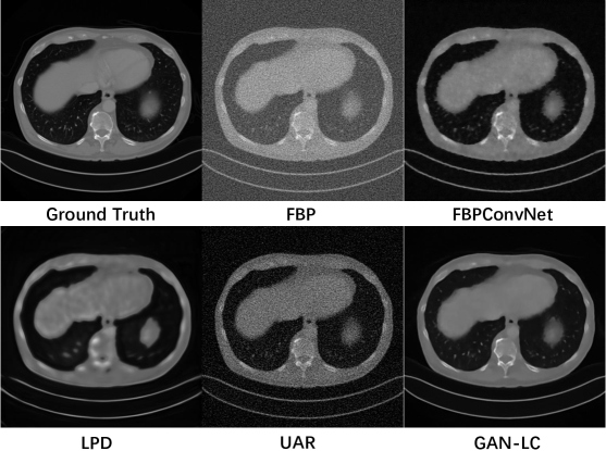
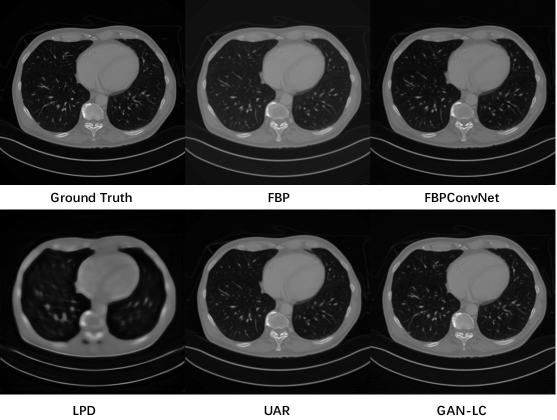
To illustrate the reconstruction performances more clearly, we also show the reconstruction results for testing images in Figure 3. We can see that our network can reconstruct the CT image with higher quality. Due to the space limit, the experimental results of different views and more visualized results are placed in our supplementary material.
| Sinograms | ||||||||
|---|---|---|---|---|---|---|---|---|
| PSNR | SSIM | PSNR | SSIM | PSNR | SSIM | PSNR | SSIM | |
| FBP | 26.449 | 0.721 | 13.517 | 0.191 | 21.460 | 0.616 | 12.593 | 0.168 |
| FBPConvNet | 38.213 | 0.918 | 30.148 | 0.743 | 35.263 | 0.869 | 29.095 | 0.723 |
| LPD | 28.050 | 0.844 | 28.357 | 0.794 | 28.376 | 0.826 | 27.409 | 0.801 |
| UAR | 33.248 | 0.902 | 22.048 | 0.272 | 29.829 | 0.848 | 21.227 | 0.238 |
| GAN-LC | 39.548 | 0.950 | 32.437 | 0.819 | 36.542 | 0.899 | 31.586 | 0.725 |
| Sinograms | ||||||||
|---|---|---|---|---|---|---|---|---|
| PSNR | SSIM | PSNR | SSIM | PSNR | SSIM | PSNR | SSIM | |
| FBP | 21.398 | 0.647 | 15.609 | 0.233 | 19.49 | 0.597 | 14.845 | 0.203 |
| FBPConvNet | 27.256 | 0.671 | 19.520 | 0.444 | 27.504 | 0.650 | 18.517 | 0.431 |
| LPD | 22.341 | 0.615 | 12.196 | 0.466 | 22.172 | 0.556 | 12.215 | 0.455 |
| UAR | 24.915 | 0.667 | 20.943 | 0.207 | 21.136 | 0.557 | 19.873 | 0.176 |
| GAN-LC | 28.861 | 0.721 | 22.624 | 0.517 | 29.171 | 0.705 | 19.607 | 0.470 |
5 Conclusion
In this paper, we propose a novel approach for low-dose CT reconstruction using generative adversarial networks with local coherence. By considering the inherent continuity of human body, local coherence can be captured through optical flow, which is small deformations and structural differences between consecutive CT slices.
The experimental results on real datasets demonstrate the advantages of our proposed network over several popular approaches.
In future, we will evaluate our network on real-world CT images from local hospital and use the reconstructed images to support doctors for the diagnosis and recognition of lung nodules.
Acknowledgements. The research of this work was supported in part by National Key R&D program of China through grant 2021YFA1000900, the NSFC throught Grant 62272432, the Provincial NSF of Anhui through grant 2208085MF163, a Huawei-USTC Joint Innovation Project on Fundamental System Software and sponsored by CAAI-Huawei MindSpore Open Fund.
References
- [1] Adler, J., Öktem, O.: Learned primal-dual reconstruction. IEEE transactions on medical imaging 37(6), 1322–1332 (2018)
- [2] Armanious, K., Jiang, C., Fischer, M., Küstner, T., Hepp, T., Nikolaou, K., Gatidis, S., Yang, B.: Medgan: Medical image translation using gans. Computerized medical imaging and graphics 79, 101684 (2020)
- [3] Beauchemin, S.S., Barron, J.L.: The computation of optical flow. ACM computing surveys (CSUR) 27(3), 433–466 (1995)
- [4] Chambolle, A.: An algorithm for total variation minimization and applications. Journal of Mathematical imaging and vision 20(1), 89–97 (2004)
- [5] Chen, H., Zhang, Y., Zhang, W., Liao, P., Li, K., Zhou, J., Wang, G.: Low-dose ct via convolutional neural network. Biomedical optics express 8(2), 679–694 (2017)
- [6] Chu, M., Xie, Y., Mayer, J., Leal-Taixé, L., Thuerey, N.: Learning temporal coherence via self-supervision for gan-based video generation. ACM Transactions on Graphics (TOG) 39(4), 75–1 (2020)
- [7] Ding, Q., Nan, Y., Gao, H., Ji, H.: Deep learning with adaptive hyper-parameters for low-dose ct image reconstruction. IEEE Transactions on Computational Imaging 7, 648–660 (2021)
- [8] Dosovitskiy, A., Fischer, P., Ilg, E., Hausser, P., Hazirbas, C., Golkov, V., Van Der Smagt, P., Cremers, D., Brox, T.: Flownet: Learning optical flow with convolutional networks. In: Proceedings of the IEEE international conference on computer vision. pp. 2758–2766 (2015)
- [9] Goodfellow, I.J., Pouget-Abadie, J., Mirza, M., Xu, B., Warde-Farley, D., Ozair, S., Courville, A.C., Bengio, Y.: Generative adversarial networks. CoRR abs/1406.2661 (2014), http://arxiv.org/abs/1406.2661
- [10] Horn, B.K., Schunck, B.G.: Determining optical flow. Artificial intelligence 17(1-3), 185–203 (1981)
- [11] Jin, K.H., McCann, M.T., Froustey, E., Unser, M.: Deep convolutional neural network for inverse problems in imaging. IEEE Transactions on Image Processing 26(9), 4509–4522 (2017)
- [12] Kak, A.C., Slaney, M.: Principles of computerized tomographic imaging. SIAM (2001)
- [13] Knoll, F., Bredies, K., Pock, T., Stollberger, R.: Second order total generalized variation (tgv) for mri. Magnetic resonance in medicine 65(2), 480–491 (2011)
- [14] Kobler, E., Effland, A., Kunisch, K., Pock, T.: Total deep variation for linear inverse problems. In: Proceedings of the IEEE/CVF Conference on Computer Vision and Pattern Recognition. pp. 7549–7558 (2020)
- [15] Li, H., Schwab, J., Antholzer, S., Haltmeier, M.: Nett: Solving inverse problems with deep neural networks. Inverse Problems 36(6), 065005 (2020)
- [16] Lin, W.A., Liao, H., Peng, C., Sun, X., Zhang, J., Luo, J., Chellappa, R., Zhou, S.K.: Dudonet: Dual domain network for ct metal artifact reduction. In: Proceedings of the IEEE/CVF Conference on Computer Vision and Pattern Recognition. pp. 10512–10521 (2019)
- [17] Liu, H., Lin, Y., Ibragimov, B., Zhang, C.: Low dose 4d-ct super-resolution reconstruction via inter-plane motion estimation based on optical flow. Biomedical Signal Processing and Control 62, 102085 (2020)
- [18] Lunz, S., Öktem, O., Schönlieb, C.B.: Adversarial regularizers in inverse problems. Advances in neural information processing systems 31 (2018)
- [19] McCann, M.T., Nilchian, M., Stampanoni, M., Unser, M.: Fast 3d reconstruction method for differential phase contrast x-ray ct. Optics express 24(13), 14564–14581 (2016)
- [20] McCollough, C.: Tu-fg-207a-04: overview of the low dose ct grand challenge. Medical physics 43(6Part35), 3759–3760 (2016)
- [21] Mira, C., Moya-Albor, E., Escalante-Ramírez, B., Olveres, J., Brieva, J., Vallejo, E.: 3d hermite transform optical flow estimation in left ventricle ct sequences. Sensors 20(3), 595 (2020)
- [22] Mukherjee, S., Carioni, M., Öktem, O., Schönlieb, C.B.: End-to-end reconstruction meets data-driven regularization for inverse problems. Advances in Neural Information Processing Systems 34, 21413–21425 (2021)
- [23] Patraucean, V., Handa, A., Cipolla, R.: Spatio-temporal video autoencoder with differentiable memory. arXiv preprint arXiv:1511.06309 (2015)
- [24] Ramm, A.G., Katsevich, A.I.: The Radon transform and local tomography. CRC press (2020)
- [25] Romano, Y., Elad, M., Milanfar, P.: The little engine that could: Regularization by denoising (red). SIAM Journal on Imaging Sciences 10(4), 1804–1844 (2017)
- [26] Ronneberger, O., Fischer, P., Brox, T.: U-net: Convolutional networks for biomedical image segmentation. In: Medical Image Computing and Computer-Assisted Intervention–MICCAI 2015: 18th International Conference, Munich, Germany, October 5-9, 2015, Proceedings, Part III 18. pp. 234–241. Springer (2015)
- [27] Rudin, L.I., Osher, S., Fatemi, E.: Nonlinear total variation based noise removal algorithms. Physica D: nonlinear phenomena 60(1-4), 259–268 (1992)
- [28] Sori, W.J., Feng, J., Godana, A.W., Liu, S., Gelmecha, D.J.: Dfd-net: lung cancer detection from denoised ct scan image using deep learning. Frontiers of Computer Science 15, 1–13 (2021)
- [29] Toft, P.: The radon transform. Theory and Implementation (Ph. D. Dissertation)(Copenhagen: Technical University of Denmark) (1996)
- [30] Venkatakrishnan, S.V., Bouman, C.A., Wohlberg, B.: Plug-and-play priors for model based reconstruction. In: 2013 IEEE Global Conference on Signal and Information Processing. pp. 945–948. IEEE (2013)
- [31] Wang, C., Shang, K., Zhang, H., Li, Q., Zhou, S.K.: Dudotrans: Dual-domain transformer for sparse-view ct reconstruction. In: Machine Learning for Medical Image Reconstruction: 5th International Workshop, MLMIR 2022, Held in Conjunction with MICCAI 2022, Singapore, September 22, 2022, Proceedings. pp. 84–94. Springer (2022)
- [32] Wang, T.C., Liu, M.Y., Zhu, J.Y., Liu, G., Tao, A., Kautz, J., Catanzaro, B.: Video-to-video synthesis. arXiv preprint arXiv:1808.06601 (2018)
- [33] Wang, Z., Bovik, A.C., Sheikh, H.R., Simoncelli, E.P.: Image quality assessment: from error visibility to structural similarity. IEEE transactions on image processing 13(4), 600–612 (2004)
- [34] Weng, N., Yang, Y.H., Pierson, R.: Three-dimensional surface reconstruction using optical flow for medical imaging. IEEE transactions on medical imaging 16(5), 630–641 (1997)
- [35] Wolterink, J.M., Leiner, T., Viergever, M.A., Išgum, I.: Generative adversarial networks for noise reduction in low-dose ct. IEEE transactions on medical imaging 36(12), 2536–2545 (2017)
- [36] Xue, T., Wu, J., Bouman, K., Freeman, B.: Visual dynamics: Probabilistic future frame synthesis via cross convolutional networks. Advances in neural information processing systems 29 (2016)
- [37] Zhao, B., James, L.P., Moskowitz, C.S., Guo, P., Ginsberg, M.S., Lefkowitz, R.A., Qin, Y., Riely, G.J., Kris, M.G., Schwartz, L.H.: Evaluating variability in tumor measurements from same-day repeat ct scans of patients with non–small cell lung cancer. Radiology 252(1), 263–272 (2009)
Appendix 0.A Supplementary figures