Robust Digital-Twin Localization via An RGBD-based Transformer Network and A Comprehensive Evaluation on a Mobile Dataset

Abstract

The potential of digital-twin technology, involving the creation of precise digital replicas of physical objects, to reshape AR experiences in 3D object tracking and localization scenarios is significant. However, enabling robust 3D object tracking in dynamic mobile AR environments remains a formidable challenge. These scenarios often require a more robust pose estimator capable of handling the inherent sensor-level measurement noise. In this paper, recognizing the challenges of comprehensive solutions in existing literature, we propose a transformer-based 6DoF pose estimator designed to achieve state-of-the-art accuracy under real-world noisy data. To systematically validate the new solution’s performance against the prior art, we also introduce a novel RGBD dataset called Digital Twin Tracking Dataset v2 (DTTD2), which is focused on digital-twin object tracking scenarios. Expanded from an existing DTTD v1 (DTTD1), the new dataset adds digital-twin data captured using a cutting-edge mobile RGBD sensor suite on Apple iPhone 14 Pro, expanding the applicability of our approach to iPhone sensor data. Through extensive experimentation and in-depth analysis, we illustrate the effectiveness of our methods under significant depth data errors, surpassing the performance of existing baselines. Code and dataset are made publicly available at: https://github.com/augcog/DTTD2.

I Introduction

Digital twin is a problem of virtually augmenting real objects with their digital models. In the context of augmented reality (AR), utilizing digital-twin representation presents challenges and complexities in real-time, accurate 3D object tracking. In contrast to the more matured technology of camera tracking in static settings known as visual odometry or simultaneous localization and mapping [7, 42, 39, 24], identifying the relative position and orientation of one or more objects with respect to the user’s ego position is a core function that would ensure the quality of user experience in digital-twin applications. In the most general setting, each object with respect to the ego position may undergo independent rigid-body motion, and the combined effect of overlaying multiple objects in the scene may also cause parts of the objects to be occluded from the measurement of the ego position. The main topic of our investigation in this paper is to study the digital-twin localization problem under the most general motion, occlusion, color, and lighting conditions.

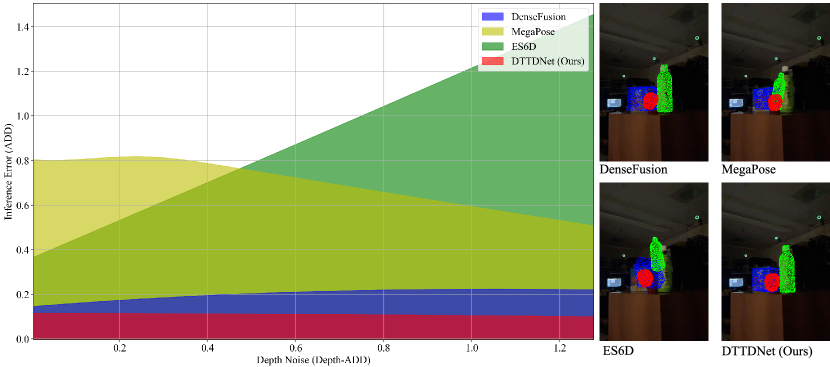
Figure 1: Left: Shadow plot of the relation between the depth noise (depth-ADD) and the max inference error (ADD) of considered state-of-the-art methods and proposed DTTDNet. Right: Visualization of pose estimation results of those methods and proposed DTTDNet.

Recent advancements in the field of 3D object tracking have primarily been motivated by deep neural network (DNN) approaches that advocate end-to-end training to carry out crucial tasks such as image semantic segmentation, object classification, and object pose estimation. Notable studies [46, 17, 16, 23, 35] have demonstrated the effectiveness of these pose estimation algorithms using established real-world 3D object tracking datasets [20, 34, 49, 32, 21, 31]. However, it should be noted that these datasets primarily focus on robotic grasping tasks, and applying these solutions to mobile AR applications introduces a fresh set of challenges. Our previous work that introduced the Digital Twin Tracking Dataset v1 (DTTD1) [10] first studied this gap in the context of 3D object localization for mobile AR applications. DTTD1 aims to replicate real-world digital-twin scenarios by expanding the capturing distance, incorporating diverse lighting conditions, and introducing varying levels of object occlusions. It is important to mention that, however, this dataset was collected using Microsoft Azure Kinect, which may not be the most suitable camera platform for mobile AR applications.

Alternatively, Apple has emerged as a strong proponent of utilizing RGB+Depth (RGBD) spatial sensors for mobile AR applications with the design of their iPhone Pro camera suite, such as on the latest iPhone 14 Pro model. This particular smartphone has been given a back-facing LiDAR depth sensor, a critical addition for mobile and wearable AR applications. LiDAR (Light Detection and Ranging) technology has revolutionized the field of 3D perception and spatial understanding, enabling machines to perceive their surroundings with exceptional accuracy and detail[22, 28, 2]. It has found a particularly significant application in the realm of 3D object tracking[11, 50, 48] as well.

Six degrees-of-freedom (6DoF) pose estimation involves determining the precise position and orientation of an object in 3D space relative to a reference coordinate system. This task is of paramount importance in various fields, including robotics[46], augmented reality[43], and autonomous driving[11, 50, 48]. Accurate and robust 6DoF pose estimation is crucial for enabling machines to interact seamlessly and safely with the physical world. However, one distinguishing drawback of the iPhone LiDAR depth is the low resolution of the depth map provided by the iPhone ARKit[39], a $256\times 192$ resolution compared to a $1280\times 720$ depth map provided by the Microsoft Azure Kinect. This low resolution is exacerbated by large errors in the retrieved depth map. The large amounts of error in the iPhone data also pose challenges for researchers to develop a pose estimator that can correctly predict object poses that rely heavily on the observed depth map.

To investigate the digital-twin localization problem under the most popular mobile depth sensor, namely, the Apple iPhone 14 Pro LiDAR, we propose an RGBD-based transformer model for 6DoF object pose estimation, which is designed to effectively handle inaccurate depth measurements and noise. As shown in Figure 1, our method shows robustness against noisy depth input, while other baselines failed in such conditions. Meanwhile, we introduce DTTD v2 (DTTD2), a novel RGBD dataset captured by iPhone 14 Pro, to bridge the gap of digital-twin pose estimation for mobile AR applications, allowing research into extending algorithms to iPhone data and analyzing the unique nature of iPhone depth sensors.

Our contributions are summarized as follows:

• We propose a new transformer-based 6DoF pose estimator with depth-robust designs on modality fusion and training strategies, called DTTDNet. The new solution outperforms other state-of-the-art methods by a large margin in noisy depth conditions.

• We introduce DTTD2 as a novel digital-twin pose estimation dataset for mobile AR applications. We provide in-depth LiDAR depth analysis and evaluation metrics to illustrate the unique properties and complexities of mobile LiDAR data while being used in mobile AR environments.

• We conducted extensive experiments and ablation studies to demonstrate the efficacy of DTTDNet and shed light on how the depth-robustifying module works.

II Related Work

II-A 6DoF Pose Estimation Algorithms

The majority of data-driven approaches for object pose estimation revolve around utilizing either RGB images [26, 38, 49, 51] or RGBD images [16, 17, 46, 35, 23] as their input source.

RGB-only approach. Studies following the RGB-only approach often rely on incorporating additional prior information and inductive biases during the inference process. These requirements impose additional constraints on the application of 3D object tracking on mobile devices. Their inference process can involve utilizing more viewpoints for similarity matching[33, 27] or geometry reconstruction[43], employing rendering techniques[27, 36, 3] based on precise 3D model or leveraging an additional database for viewpoint encoding retrieval[3]. During the training phase, these approaches typically draw upon more extensive datasets, such as synthetic datasets, to facilitate effective generalization within open-set scenarios. However, when confronted with a limited set of data samples, their performance does not surpass that of closed-set algorithms in cases where there is a surplus of prior information available and depth map loss.

RGBD approach. On the other hand, methods[16, 17, 46, 35, 23] that relied on depth maps advocated for the modality fusion of depth and RGB data to enhance their inference capabilities. To effectively fuse multi-modalities, Wang et al. [46] introduced a network architecture capable of extracting and integrating dense feature embedding from both RGB and depth sources. Due to its simplicity, this method achieved high efficiency in predicting object poses. In more recent works [17, 16, 18], performance improvements were achieved through more sophisticated network architectures. For instance, He et al. [16] proposed an enhanced bidirectional fusion network for key-point matching, resulting in high accuracy on benchmarks such as YCB-Video [49] and LINEMOD [20]. However, these methods exhibited reduced efficiency due to the complex hybrid network structures and processing stages. Addressing symmetric objects, Mo et al. [35] proposed a symmetry-invariant pose distance metric to mitigate issues related to local minima. On the other hand, Jiang et al. [23] proposed an L1-regularization loss named abc loss, which enhanced pose estimation accuracy for non-symmetric objects.

II-B 3D Object Tracking Datasets

Existing object pose estimation algorithms are predominantly tested on a limited set of real-world 3D object tracking datasets [20, 34, 49, 32, 21, 31, 10, 5, 6, 4], which often employ depth-from-stereo sensors or time-of-flight (ToF) sensors for data collection. Datasets like YCB-Video[49], LINEMOD[20], StereoOBJ-1M[31], and TOD[32] utilize depth-from-stereo sensors, while TLess[21] and our prior work DTTD1 [10] deploy ToF sensors, specifically the Microsoft Azure Kinect, to capture meter-scale RGBD data. However, the use of cameras with depth-from-stereo sensors may not be an optimal platform for deploying AR software, because stereo sensors may degrade rapidly in longer-distance [13] and may encounter issues with holes in the depth map when stereo matching fails.

However, it is essential to note that our choice of the iPhone 14 Pro, while different from the Azure Kinect, presents its own unique advantages and challenges. In our pursuit of addressing the limitations of existing datasets and ensuring a more realistic dataset for AR applications in household scenarios, particularly for mobile devices, we opt to collect RGBD data using the iPhone 14 Pro. By leveraging the iPhone 14 Pro’s LiDAR ToF sensor, our dataset can provide more accurate and reliable depth information while catering to a broader range of real-world occlusion and lighting conditions, thereby enhancing the robustness and practicality of data-driven object pose estimation algorithms.

II-C iPhone-based Datasets for 3D Applications

There are several datasets that utilize the iPhone as their data collection device for 3D applications, such as ARKitScenes[1], MobileBrick[29], ARKitTrack[52], and RGBD Dataset[15]. These datasets were constructed to target applications from 3D indoor scene reconstruction, 3D ground-truth annotation, depth-map pairing from different sensors, to RGBD tracking in both static and dynamic scenes. However, most of these datasets did not specifically target the task of 6DoF object pose estimation. Our dataset provides a distinct focus on this task, offering per-pixel segmentation and pose labels. This enables researchers to delve into the 3D localization tasks of objects with a dataset specifically designed for this purpose.

The most relevant work is from OnePose[43], which is an RGBD 3D dataset collected by iPhone. However, their dataset did not provide 3D models for close-set settings, and they utilized automatic localization provided by ARKit for pose annotation, which involved non-trivial error for high-accuracy 6DoF pose estimation. On the other hand, we achieve higher localization accuracy with OptiTrack professional motion capture system to track the iPhone camera’s real-time positions as it moves in 3D.

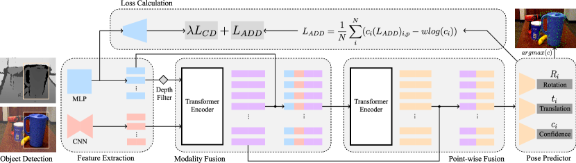
Figure 2: Model Architecture Overview. DTTDNet pipeline starts with segmented depth maps and cropped RGB images. The point cloud from the depth map and RGB colors are encoded and integrated point-wise. Extracted features are then fed into an attention-based two-stage fusion. Finally, the pose predictor produces point-wise predictions with both rotation and translation.

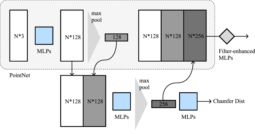
Figure 3: Detailed model architecture for point-cloud auto-encoder in DTTDNet. The 128-D point-wise feature undergoes max pooling to obtain a global feature representation. Subsequently, these two features are aggregated and further encoded to yield a 256-D representative embedding.

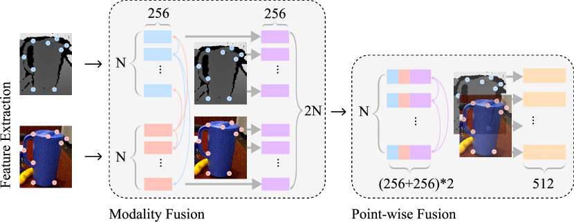
Figure 4: Diagram of attention mechanism in the fusion process in DTTDNet. Modality fusion module utilizes the embedding from unimodal encoders and feeds them into a transformer encoder in parallel for cross-modal fusion. The latter point-wise fusion module relies on similarity scores among points.

III Methods

In this section, we will elaborate on the specific details of our methods. The objective is to estimate the 3D location and pose of a known object in the camera coordinates from the RGBD images. This position can be represented using homogeneous transformation matrix $p\in SE(3)$, which consists of a rotation matrix $R\in SO(3)$ and a translation matrix $t\in\mathbb{R}^{3}$, $p=[R|t]$. Section III-A describes our transformer-based model architecture. Section III-B introduces two depth robustifying modules on depth feature extractions, dedicated to geometric feature reconstruction and filtering. Section III-C illustrates our modality fusion design for the model to disregard significant noisy depth feature. Finally, Section III-D describes our final learning objective.

III-A Architecture Overview

Figure 2 illustrates the overall architecture of the proposed DTTDNet. The DTTDNet pipeline takes segmented depth maps and cropped RGB images as input. It then obtains feature embedding for both RGB and depth images through separate CNN and point-cloud encoders on cropped RGB images and reconstructed point cloud corresponding to the cropped depth images. For RGB feature extraction, the image embedding network comprises a ResNet-18 encoder, which is then followed by 4 up-sampling layers acting as the decoder. It translates an image of size $H\times W\times 3$ into a $H\times W\times d_{rgb}$ embedding space. For depth feature extraction, we take segmented depth pixels and transform them into 3D point clouds with the camera intrinsics.

The 3D point clouds are initially processed using an auto-encoder (Figure 3) inspired by the PointNet [40]. The PointNet-style encoding step aims to capture geometric representations in latent space in $\mathbb{R}^{d_{1}}$. In this context, the encoder component produces two sets of features: early-stage point-wise features in $\mathbb{R}^{N\times d_{2}}$ and global geometric features in $\mathbb{R}^{d_{3}}$. Subsequently, we add a decoder which is guided by a reference point set $P$ to generate the predicted point cloud $\hat{P}$. Features extracted from the encoder are subsequently combined with the learned representations to create a new feature sequence with a dimension of $\mathbb{R}^{N\times d_{geo}}$, where $d_{geo}=d_{1}+d_{2}+d_{3}$.

This results in a sequence of geometric tokens with a length equal to the number of points $N$. Extracted RGB and depth features are then fed into a two-stage attention-based fusion block, which consists of modality fusion and point-wise fusion. Finally, the pose predictor produces point-wise predictions with both rotation and translation. The predictions are then voted based on unsupervised confidence scoring to get the final 6DoF pose estimate.

III-B Depth Data Robustifying

In this section, we will introduce two modules, Chamfer Distance Loss (CDL) and Geometric Feature Filtering (GFF), that enable the point-cloud encoder in DTTDNet to better handle noisy and low-resolution LiDAR data in a robust way.

Chamfer Distance Loss (CDL). Past methods either treated the depth information directly as image channels[35] or directly extracted features from a point cloud for information extraction[46]. These methods underestimated the corruption of the depth data caused by noise and error during the data collection process.

To address this, we first introduce a downstream task for point-cloud reconstruction and utilize the Chamfer distance as a loss function to assist our feature embedding in filtering out noise. The Chamfer distance loss (CDL) is widely used for denoising in 3D point clouds [19, 9], and it is defined as the following equation between two point clouds $P\in\mathbb{R}^{N\times 3}$ and $\hat{P}\in\mathbb{R}^{N\times 3}$:

where $\hat{P}$ denotes the decoded point set from the embedding, and $P$ denotes the reference point set employed to guide the decoder’s learning.

We present two distinct alternatives for supervising the decoder: The first option involves the point cloud extracted from the depth map, whereas the second option involves using the point cloud sampled from the object model. While the former is tailored to reduce the noise of the depth map, the latter focuses on representing the object’s geometry, ensuring a robust depth data representation.

Geometric Feature Filtering (GFF). Due to the non-Gaussian noise distribution in iPhone LiDAR data (Figure 7), which should be assumed for most depth camera data, normal estimators might either get perturbed by such noisy features or interpret wrong camera-object rotations. To deal with this sensor-level error, we advocate for the integration of a Geometric Feature Filtering (GFF) module prior to the modality fusion module. Drawing inspiration from the Filter-Enhanced MLPs used in the sequential recommendation [53], our approach incorporates the Fast Fourier Transform (FFT) into the geometric feature encoding. Specifically, the GFF module includes an FFT, a subsequent single layer of MLP, and finally, an inverse-FFT. By leveraging FFT, we are able to transpose the input sequence of geometric signals to the frequency domain, which selects significant features from noisy input signals. After that, we obtain a more refined geometric embedding that is resilient to the non-Gaussian iPhone LiDAR noise.

III-C Attention-based RGBD Fusion

Previous papers have emphasized the importance of modality fusion [16, 46] and the benefits of gathering nearest points from the point cloud [35, 16] in RGBD-based pose estimation tasks. While the feature extractor widens each point’s receptive field, we aim for features to interact beyond their corresponding points [46] or neighboring points [16]. In predicting the 6DoF pose of a cuboid based on multiple feature descriptors, our focus is on attending to various corner points, rather than solely those in close proximity to each other. To this end, inspired by recent transformer-based models used for modality fusion [8, 14, 37, 30, 41, 25, 47], we leverage the self-attention mechanism [45] to amplify and integrate important features while disregarding the significant LiDAR noise. Specifically, our fusion part is divided into two stages: modality fusion and point-wise fusion (Figure 4). Both of our fusion modules consist of a standard transformer encoder with linear projection, multi-head attention and layer norm. The former module utilizes the embedding from single-modal encoders and feeds them into a transformer encoder in parallel for cross-modal fusion. The latter fusion module relies on similarity scores among points. It merges all feature embedding in a point-wise manner before feeding them into a transformer encoder.

Modality Fusion. The objective of this module is to combine geometric embedding $g$ and RGB embedding $c$ produced by single-modal encoders in a cross-modal fashion. Drawing inspiration from ViLP [25], both types of embedding are linearly transformed into a token sequence ($\in\mathbb{R}^{N\times d_{emb}}$). Before entering the modality fusion module $E_{1}$, these features are combined along the sequence length direction, i.e., all feature embedding is concentrated into a single combined sequence, where the dimension remains $d_{emb}$, and the sequence length becomes twice the original length (Figure 4).

$$f_{1}=E_{1}\left[c\oplus g\right]\in\mathbb{R}^{d_{f_{1}}\times 2N},$$

where the operation symbol ”$\oplus$” denotes concentrating along the row direction. It is then reshaped into the sequence $f_{1}^{\prime}$ with the length of N and dimension of $2d_{f_{1}}$ in order to adapt the point-wise transformer encoder in the next fusion stage. This step enables the model’s attention mechanism to effectively perform cross-modal fusion tasks.

Point-Wise Interaction. The goal of this stage is to enhance the integration of information among various points. The primary advantage of our method over the previous work[16] is that our model can calculate similarity scores not only with the nearest point but also with all other points, allowing for more comprehensive interactions. In order to enable the point-wise fusion to effectively capture the similarities between different points, we merge the original RGB token sequence $c$ and the geometric token sequence $g$ together with the output embedding sequence $m^{\prime}$ from the modality fusion module along the feature dimension direction. The combined sequence input $\left[c^{T}\oplus g^{T}\oplus(f_{1}^{\prime})^{T}\right]^{T}\in\mathbb{R}^{(2d_{emb}+2d_{f_{1}})\times N}$ is then fed into the point-wise transformer encoder $E_{2}$ to acquire the final fusion:

$$f_{2}=E_{2}\left[c^{T}\oplus g^{T}\oplus(f_{1}^{\prime})^{T}\right]^{T}\in\mathbb{R}^{d_{f_{2}}\times N}.$$

Attention Mechanism. For both modality fusion and point-wise fusion stage, the scaled dot-product attention is utilized in the self-attention layers:

$$s_{i,j}=\mathbf{q}_{i}^{T}\mathbf{k}_{j}/\sqrt{d_{\text{head}}};$$

$$a_{i,j}=\dfrac{\exp(s_{i,j})}{\sum_{k}\exp(s_{i,k})};$$

$$\mathrm{Attention}(\mathbf{Q},\mathbf{K},\mathbf{V})_{i}=\sum_{j}a_{i,j}\mathbf{v}_{j},$$

where query, key, value, and similarity score are denoted as $q$, $k$, $v$, and $s$. The distinction between two fusion stages lies in the token preparation prior to the linear projection layer. It results in varying information contained within the query, key, and value.

The key idea in the first fusion stage is to perform local per-point fusion in a cross-modality manner so that we can make predictions based on each fused feature. Each key or query carries only one type of modal information before fusion, allowing different modalities to equally interact with each other through dot-product operations. It exerts a stronger influence when the RGB and geometric representations produce higher similarity.

In the second stage, where we integrate two original single-modal features with the first-stage feature into each point, we calculate similarities solely among different points. The key idea is to enforce attention layers to further capture potential relationships among multiple local features. A skip connection is employed in a concentrating manner between two fusion outputs so that we can make predictions based on per-point features generated in both the first and second stages.

III-D Learning Objective

Based on the overall network structure, our learning objective is to perform 6DoF pose regression, which measures the disparity between points sampled on the object’s model in its ground truth pose and corresponding points on the same model transformed by the predicted pose. Specifically, the pose estimation loss is defined as:

$$(L_{ADD})_{i,p}=\frac{1}{m}\sum_{x\in M}\|(Rx+t)-(\hat{R_{i}}x+\hat{t_{i}})\|$$ (2)

where $M\in\mathbb{R}^{m\times 3}$ represents the randomly sampled point set from the object’s 3D model, $p=[R|t]$ denotes the ground truth pose, and $\hat{p_{i}}=[\hat{R_{i}}|\hat{t_{i}}]$ denotes the predicted pose generated from the fused feature of the $i^{th}$ point. Our objective is to minimize the sum of the losses for each fusion point, which can be expressed as $L_{ADD}=\frac{1}{N}\sum_{i}^{N}(L_{ADD})_{i,p}$, where $N$ is the number of randomly sampled points (token sequence length in the point-wise fusion stage). Meanwhile, we introduce a confidence regularization score ($c_{i}$) along with each prediction $\hat{p_{i}}=[\hat{R_{i}}|\hat{t_{i}}]$, which denotes confidence among the predictions for each fusion point:

$$L_{ADD}=\frac{1}{N}\sum_{i}^{N}(c_{i}(L_{ADD})_{i,p}-wlog(c_{i}))$$ (3)

Predictions with low confidence will lead to a low ADD loss, but this will be balanced by a high penalty from the second term with hyper-parameter $w$. Finally, the CDL loss, as outlined in Section III-B, undergoes joint training throughout the training process, leading us to derive our ultimate learning objective as follows:

$$L=L_{ADD}+\lambda L_{CD}$$ (4)

where $\lambda$ denotes the weight of the CDL loss.

TABLE I: Features and statistics of different datasets.

Dataset	Modality	iPhone Camera	Texture	Occlusion	Light variation	# of frames	# of scenes	# of objects	# of annotations
StereoOBJ-1M[31]	RGB	$\times$	$\checkmark$	$\checkmark$	$\checkmark$	393,612	182	18	1,508,327
LINEMOD[20]	RGBD	$\times$	$\checkmark$	$\checkmark$	$\times$	18,000	15	15	15,784
YCB-Video[49]	RGBD	$\times$	$\checkmark$	$\checkmark$	$\times$	133,936	92	21	613,917
DTTD1[10]	RGBD	$\times$	$\checkmark$	$\checkmark$	$\checkmark$	55,691	103	10	136,226
TOD[32]	RGBD	$\times$	$\checkmark$	$\times$	$\times$	64,000	10	20	64,000
LabelFusion[34]	RGBD	$\times$	$\checkmark$	$\checkmark$	$\checkmark$	352,000	138	12	1,000,000
T-LESS[21]	RGBD	$\times$	$\times$	$\checkmark$	$\times$	47,762	-	30	47,762
DTTD2 (Ours)	RGBD	$\checkmark$	$\checkmark$	$\checkmark$	$\checkmark$	47,668	100	18	114,143

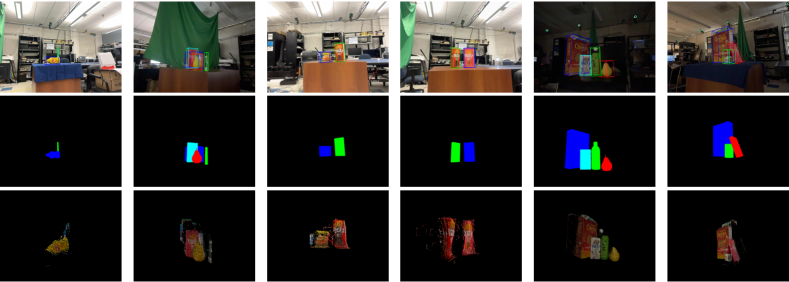
Figure 5: Sample visualizations of our dataset. First row: Annotations for 3D bounding boxes. Second row: Corresponding semantic segmentation labels. Third row: Zoomed-in LiDAR depth visualizations.

IV Dataset Description

DTTD2 data contain 18 rigid objects along with their textured 3D models. The data are generated from 100 scenes, each of which features one or more of the objects in various orientations and occlusion. The dataset offers ground-truth labels for 3D object poses and per-pixel semantic segmentation. Additionally, it provides detailed camera specifications, pinhole camera projection matrices, and distortion coefficients. Detailed features and statistics are presented in Table I. The fact that DTTD2 dataset includes multiple sets of geometrically similar objects, each having distinct color textures, poses challenges to existing digital-twin localization solutions. In order to ensure compatibility with other existing datasets, some of the collected objects partially overlap with the YCB-Video [49] and DTTD1 [10] datasets.

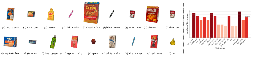
Figure 6: Left: 3D models of the 18 objects in DTTD2. Right: Quantity of scenes in which objects appear in DTTD2.

IV-A Data Acquisition

Apple’s ARKit framework enables us to capture RGB images from the iPhone camera and scene depth information from the LiDAR scanner synchronously. We leverage ARKit APIs to retrieve $1920\times 1440$ RGB images and $256\times 192$ depth maps at a capturing rate of 30 frames per second. Despite the resolution difference, both captured RGB images and depth maps match up in the aspect ratio and describe the same scene. Alongside each captured frame, DTTD2 stores the camera intrinsic matrix and lens distortion coefficients, and also stores a 2D confidence map describing how the iPhone depth sensor is confident about the captured depth at the pixel level. In practice, we disabled the auto-focus functionality of the iPhone camera during data collection to avoid drastic changes in the camera’s intrinsics between frames, and we resized the depth map to the RGB resolution using nearest neighbor interpolation to avoid depth map artifacts.

To track the iPhone’s 6DoF movement, we did not use the iPhone’s own world tracking SDK. Instead, we follow the same procedure as in [10] and use the professional OptiTrack motion capture system for higher accuracy. For label generation, we also use the open-sourced data annotation pipeline provided by [10] to annotate and refine ground-truth poses for objects in the scenes along with per-pixel semantic segmentation. Some visualizations of data samples are illustrated in Figure 5. Notice that the scenes cover various real-world occlusion and lighting conditions with high-quality annotations. Following previous dataset protocols [10, 49], we also provide synthetic data for scene augmentations used for training.

The dataset also provides 3D models of the 18 objects as illustrated in Figure 6. These models are reconstructed using the iOS Polycam app via access to the iPhone camera and LiDAR sensors. To enhance the models, Blender is employed to repair surface holes and correct inaccurately scanned texture pixels.

IV-B Benchmark and Evaluation

Train/Test Split. DTTD2 offers a suggested train/test partition as follows. The training set contains 8622 keyframes extracted from 88 video sequences, while the testing set contains 1239 keyframes from 12 video sequences. To ensure a representative distribution of scenes with occluded objects and varying lighting conditions, we randomly allocate them across both the training and testing sets. Furthermore, for training purposes of scene augmentations, we provide 20,000 synthetic images by randomly placing objects in scenes using the data synthesizer provided in [10].

Evaluation Metrics. We evaluate baseline methods with the average distance metrics ADD and ADD-S according to previous protocols[49, 10]. Suppose $R$ and $t$ are ground truth rotation and translation and $\tilde{R}$ and $\tilde{t}$ are the predicted counterparts. The ADD metric computes the mean of the pairwise distances between the 3D model points using ground truth pose $(R,t)$ and predicted pose $(\tilde{R},\tilde{t})$:

$$\mathrm{ADD}=\frac{1}{m}\sum_{x\in M}\|(Rx+t)-(\tilde{R}x+\tilde{t})\|,$$ (5)

where $M$ denotes the point set sampled from the object’s 3D model and $x$ denotes the point sampled from $M$.

The ADD-S metric is designed for symmetric objects when the matching between points could be ambiguous:

$$\mathrm{ADD{-}S}=\frac{1}{m}\sum_{x_{1}\in M}\min_{x_{2}\in M}\|(Rx_{1}+t)-(\tilde{R}x_{2}+\tilde{t})\|.$$ (6)

Following previous protocols [49, 46, 31, 33, 27], a 3D pose estimation is deemed accurate if the average distance error falls below a predefined threshold. Two widely-used metrics are employed in our work, namely ADD/ADD-S AUC and ADD/ADD-S(1cm). For commonly used ADD/ADD-S AUC, we calculate the Area Under the Curve (AUC) of the success-threshold curve over different distance thresholds, where the threshold values are normalized between 0 and 1. On the other hand, ADD/ADD-S(1cm) is defined as the percentage of pose error smaller than the 1cm threshold.

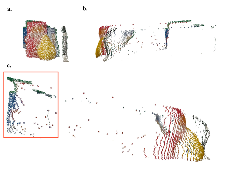
Figure 7: Visualization of an iPhone LiDAR depth scene that shows distortion and long-tail non-Gaussian noise (highlighted inside the red box). (a) Front view. (b) Left view. (c) Right view.

IV-C iPhone 14 Pro LiDAR Analysis

Compared to dedicated depth cameras such as the Microsoft Azure Kinect or Intel Realsense, iPhone 14 Pro LiDAR exhibits more noise and lower resolution at $256\times 192$ depth maps, which leads to high magnitudes of distortion on objects’ surfaces. Additionally, it introduces long-tail noise on the projection edges of objects when performing interpolation operations between RGB and depth features. Figure 7 demonstrates one such example of iPhone 14 Pro’s noisy depth data.

To further quantitatively assess the depth noise of each object from the iPhone’s LiDAR, we analyze the numerical difference between LiDAR-measured depth map, which is acquired directly from iPhone LiDAR, and reference depth map, which is derived through ground truth pose annotations. Specifically, to obtain the reference depth map, we leverage ground truth annotated object poses to render the depth projections of each object. We then apply the segmentation mask associated with each object to filter out depth readings that might be compromised due to occlusion. To measure the difference between ground truth and reference depth map, we introduce the depth-ADD metric, which calculates the average of pixel-wise L1 distance between the ground truth depth map and the reference depth map in each frame. The depth-ADD value of each object at frame $n$ is calculated as follows:

$$\mathrm{depth{-}ADD}_{n}=\frac{1}{d}\sum_{i\in D}\left|\mathrm{depth_{LiDAR}}_{i}-\mathrm{depth_{ref}}_{i}\right|,$$ (7)

where $D$ denotes the LiDAR depth map and $i$ denotes the index of pixels on it. $\mathrm{depth_{LiDAR}}_{i}$ and $\mathrm{depth_{ref}}_{i}$ represent the depth values from $D$ and the corresponding depth value from the reference depth map. The set $D$ encompasses all indices $i$ under an object’s segmentation mask where both $\mathrm{depth_{LiDAR}}_{i}$ and $\mathrm{depth_{ref}}_{i}$ yield values greater than zero. The final depth-ADD value of each object is the average of such measurement across all $N$ frames:

$$\mathrm{depth{-}ADD}=\frac{1}{N}\sum_{n\in N}\mathrm{depth{-}ADD}_{n}$$ (8)

Figure 8 shows the depth-ADD evaluation of each sampled object. Greater depth-ADD values indicate increased distortions and the presence of long-tail noise in the depth data. Our analysis indicates that the mean depth-ADD across all objects is around 0.25m. It is worth noticing that the depth quality varies significantly and could potentially be affected by outliers. For example, there are three objects: black_marker, blue_marker and pink_marker exhibiting greater errors in comparison with the other objects.

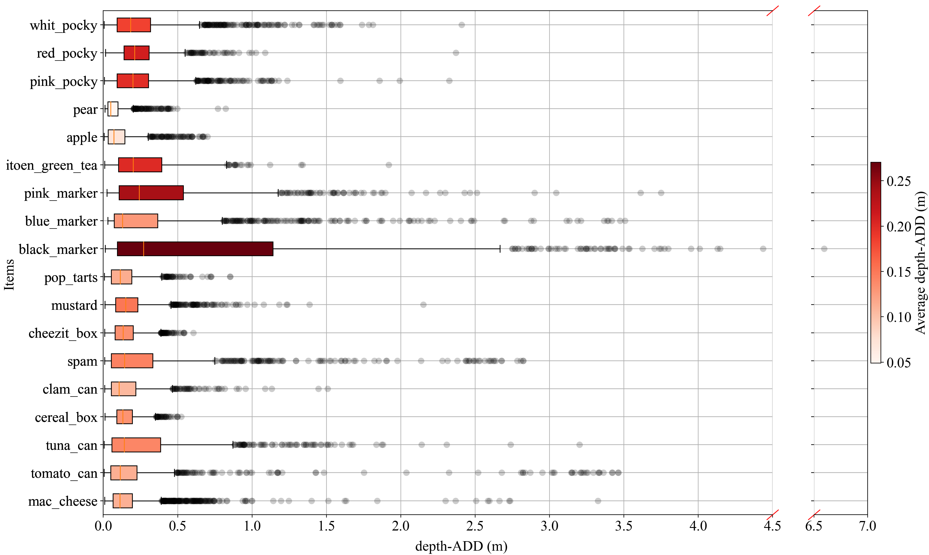
Figure 8: Box Plot of Depth Analysis Results of 18 Objects. Evaluating depth quality for objects in our iPhone dataset, the redness signifies the average depth-ADD for each item. The rectangular box denotes the interquartile range (IQR, spanning 25-75%). Whiskers highlight the typical range, either $Q1-1.5\times IQR$ or $Q3+1.5\times IQR$. Points beyond the whiskers are identified as outliers. Notably, the object black_marker exhibits poor depth qualities.

V Experiments

TABLE II: Comparison with diverse 6DoF pose estimation baselines on DTTD2 dataset. We showcase AUC results of ADD-S and ADD on all 18 objects, higher is better. Based on considered 3 baselines, our model significantly improve the accuracy and robustness on most objects.

	DenseFusion[46]		MegaPose-RGBD[27]		ES6D[35]		DTTDNet (Ours)
Object	ADD AUC	ADD-S AUC	ADD AUC	ADD-S AUC	ADD AUC	ADD-S AUC	ADD AUC	ADD-S AUC
mac_cheese	88.10	93.17	78.98	87.94	28.29	57.06	94.06	97.02
tomato_can	69.10	93.42	68.85	84.48	19.07	56.17	74.23	94.01
tuna_can	42.90	79.94	8.90	22.11	10.74	26.86	62.98	87.05
cereal_box	75.20	88.12	59.89	71.53	10.09	53.92	86.55	92.74
clam_can	90.49	96.32	74.11	90.45	17.75	35.92	88.15	96.92
spam	53.29	91.14	72.35	86.16	3.17	13.74	52.81	90.83
cheez-it_box	82.73	92.10	89.18	94.83	7.81	37.14	87.03	93.91
mustard	78.41	91.31	76.08	85.38	21.89	52.56	84.06	92.15
pop-tarts_box	82.94	92.58	44.36	58.97	3.44	35.26	84.55	92.65
black_marker	32.22	38.72	17.38	34.15	2.12	3.72	44.08	53.50
blue_marker	66.06	74.80	6.87	12.46	16.88	41.46	50.88	61.69
pink_marker	56.46	67.86	47.84	58.59	1.59	7.01	64.18	73.00
itoen_green_tea	64.37	93.10	48.43	70.50	8.80	32.86	64.59	92.31
apple	68.97	91.13	32.85	76.43	31.65	58.46	82.45	94.80
pear	65.66	91.31	35.80	56.73	16.93	32.57	47.83	88.11
pink_pocky	50.64	67.17	8.69	18.25	0.77	1.93	61.40	82.33
red_pocky	88.14	93.76	76.49	84.56	25.32	51.16	90.00	95.24
white_pocky	89.55	94.27	42.83	54.65	17.19	47.45	90.83	94.70
Average	69.67	85.88	49.02	62.44	13.25	37.38	73.99	88.10

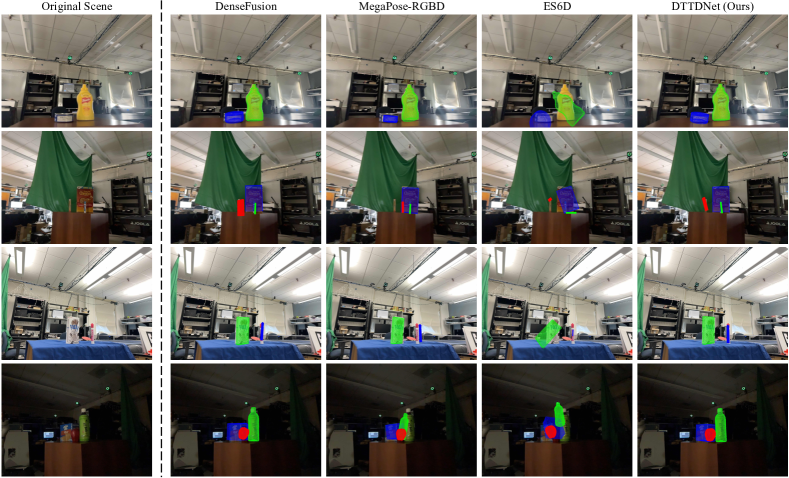
Figure 9: Qualitative evaluation of different methods. To further validate our approach, we provide visual evidence of our model’s effectiveness in challenging occlusion scenarios and varying lighting conditions, where other models’ predictions fail but ours remain reliable.

V-A Experimental Results

In this section, we compare the performance of our method DTTDNet with three other 6DoF pose estimators, namely, DenseFusion[46], MegaPose[27], ES6D[35]. While all four methods leverage the benefits of multimodal data from both RGB and depth sources, they differ in the extent to which they emphasize the depth data processing module. Quantitative experimental results are shown in Table II. Qualitative examples are shown in Figure 9.

DenseFusion[46] treats both modalities equally and lacks a specific design for the depth module, whereas ES6D[35] heavily relies on depth data during training, using grouped primitives to prevent point-pair mismatch. However, due to potential interpolation errors in the depth data, this additional supervision can introduce erroneous signals to the estimator, resulting in inferior performance compared to DenseFusion[46]. DenseFusion[46] achieves 69.67 ADD AUC and 85.88 ADD-S AUC, whereas ES6D[35] only achieves 13.25 ADD AUC and 37.38 ADD-S AUC.

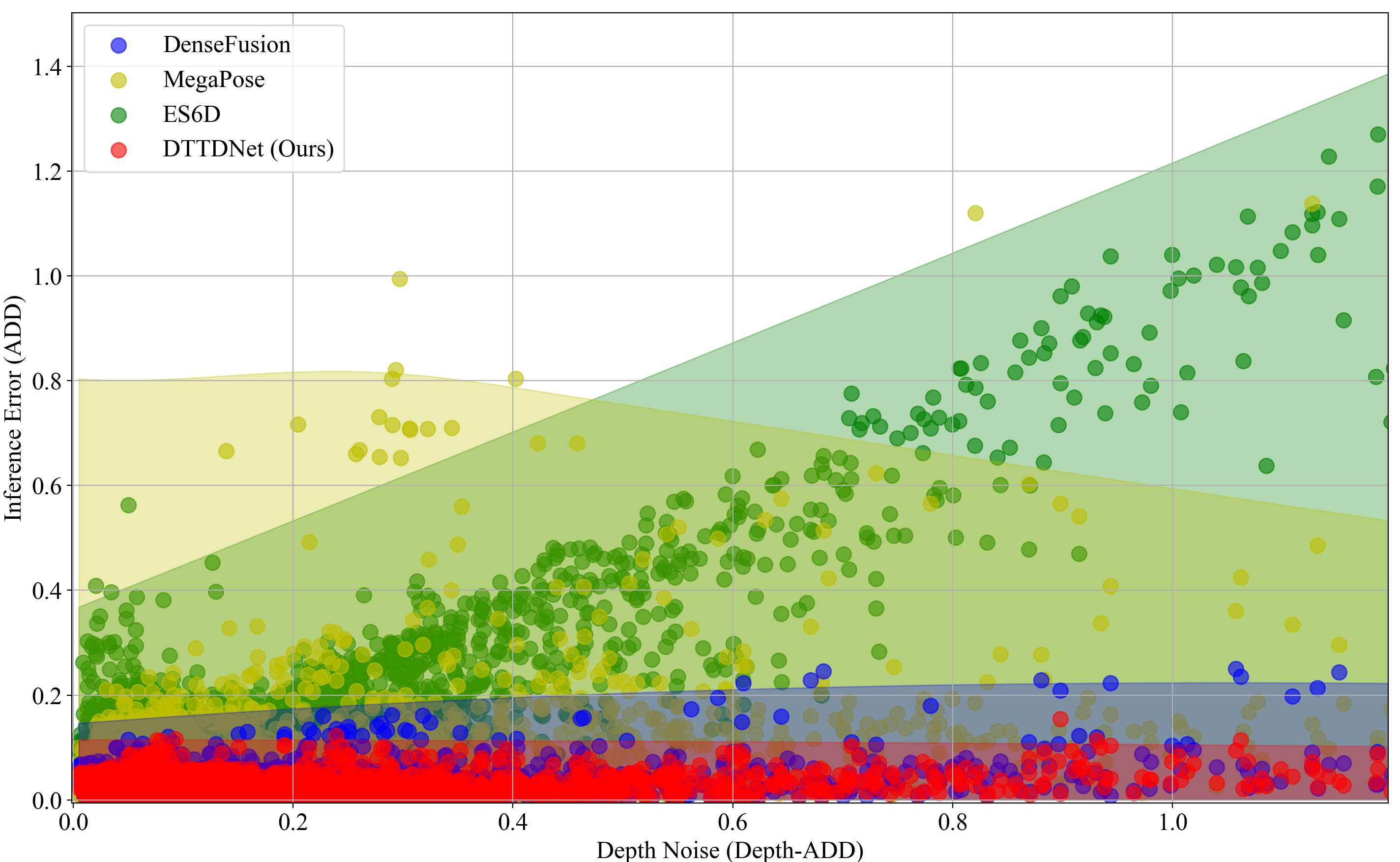
Figure 10: Scatter plot of the relation between the depth noise (depth-ADD) and the inference error (ADD) of DTTDNet and the baselines.

MegaPose[27] employs a coarse-to-fine process for pose estimation. The initial ”coarse” module leverages both RGB and depth data to identify the most probable pose hypothesis. Subsequently, a more precise pose inference is achieved through the ”render-and-compare” technique. Disregarding the noise in the depth data can also impair the effectiveness of their coarse module, consequently leading to failure in their refinement process. Even with the assistance of a refiner, MegaPose-RGBD[27] only manages to attain an ADD AUC of 49.02 and an ADD-S AUC of 62.44. Its damage and susceptibility to depth noise falls somewhere between DenseFusion[46] and ES6D[35].

In contrast, our approach harnesses the strengths of both RGB and depth modalities while explicitly designing robust depth feature extraction and selection. In comparison with the above baselines, our method achieves 73.31 ADD AUC and 87.82 ADD-S AUC, surpassing the state of the art with improvements of 1.94 and 3.64 percent in terms of ADD AUC and ADD-S AUC, respectively.

V-B Implementation Details

We extracted $1000$ of pixels from the decoded RGB representation corresponding to the same number of points in the LiDAR point set. Both extracted RGB and geometric features are linear projected to 256-D before fused together. In the above experiment results, we utilized an 8-layer transformer encoder with 4 attention heads for the modality fusion stage and a 4-layer transformer encoder with 8 attention heads for the point-wise fusion stage. In addition, a filter-enhaced MLP layer and the CDL with objects’ CAD model were considered in the above experiment results.

V-C Training Strategy

For our DTTDNet, learning rate warm-up schedule is used to ensure that our transformer-based model can overcome local minima in early stage and be more effectively trained. By empirical evaluation, in the first epoch, the learning rate $lr$ linearly increases from $0$ to $1e{-5}$. In the subsequent epochs, it is decreased using a cosine scheduler to the end learning rate $min\_lr=1e{-6}$. Additionally, following the approach of DenseFusion[46], we also decay our learning rate by a certain ratio when the average error is below a certain threshold during the training process. Detailed code and parameters will be publicly available in our code repository. Moreover, we set the importance factor $\lambda$ of CDL to $0.3$ and the initial balancing weight $w$ to $0.015$ by empirical testing.

V-D Robustness to LiDAR Depth Error

To answer the question of whether our method exhibits robustness in the presence of significant LiDAR sensor noise when compared to other approaches, we further assess the depth-ADD metric, as discussed in Section IV-C, on DTTDNet versus the three baseline algorithms. Figure 10 illustrates the correlation between the model performance (ADD) of four methods and the quality of depth information (depth-ADD) across various scenes, frames, and 1239 pose prediction outcomes for the 18 objects. Our approach ensures a stable pose prediction performance, even when the depth quality deteriorates, maintaining consistently low levels of ADD error overall. However, other methods experience deterioration in model prediction results with increasing LiDAR noise, resulting in an increase in ADD error. This is particularly evident in the case of ES6D[35], where there is a linearly increasing relationship between prediction error and LiDAR measurement error.

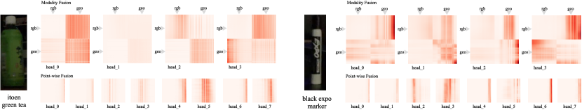
Figure 11: Examples of attention map output visualize of both modality fusion stage (the larger maps in the first row) and point-wise fusion stage (the smaller ones in the second row) on two objects (itogen_green_tea and black_marker). Due to the different ways we concentrate features in the two fusion stages, the token sequence length in modality fusion is twice that in the point-wise fusion process. For the attention maps produced in the final layer of modality fusion and point-wise fusion, they are of sizes $2000\times 2000$ and $1000\times 1000$, respectively.

VI Ablation Studies

In this section, we further delve into a detailed analysis of our own model, highlighting the utility of our depth robustifying module in handling challenging scenarios with significant LiDAR noise. Specifically, we are concerned with the following questions:

1. Throughout the entire fusion process, what did the multi-head attention layers learn at different stages?

2. Will the increase in the layer number and parameter number of the transformer encoder affect the performance of our model?

3. What role does our depth robustifying module play?

VI-A Attention Map Visualization

To visualize what our fusion module learns during the training process, we draw on previous studies [44, 12] and represent our attention map as $a_{i,j}$ described in section III-C. Taking two objects (itoen_green_tea and black_marker) as examples, Figure 11 displays the attention maps produced by different attention heads in the two fusion stages. We showcase the attention maps generated by the modality fusion and point-wise fusion at their respective final layers. The modality fusion part reveals distinct quadrant-like patterns, reflecting differences in how the two modalities fuse. The lower-left and upper-right quadrants offer insights into the degree of RGB and geometric feature fusion. The point-wise fusion part exhibits a striped pattern and shows that it attends to the significance of specific tokens during training.

TABLE III: Effect of Layer Number in 2 Fusion Stages. It shows DTTDNet with different layer number combinations in the fusion stages with one $\circ$ denoting one layer. For all combinations, CDL is used in the geometric feature extraction stage.

Layer Num of #		Metrics
Modality Fusion	Point-wise Fusion	ADD AUC	ADD-S AUC	ADD(1cm)	ADD-S(1cm)
$\circ\circ$	$\circ$	70.73	85.42	22.91	67.75
$\circ\circ$	$\circ\circ$	71.37	86.69	15.74	64.44
$\circ\circ$	$\circ\circ$$\circ\circ$	72.06	86.37	19.57	68.37
$\circ\circ$	$\circ$	70.73	85.42	22.91	67.75
$\circ\circ$$\circ\circ$	$\circ\circ$	71.76	88.23	20.01	69.03
$\circ\circ$$\circ\circ$$\circ\circ$$\circ\circ$	$\circ\circ$$\circ\circ$	72.03	86.44	19.86	70.50

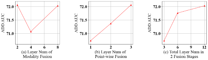
Figure 12: Effect of Fusion Layer Number on Performance. Left: the ADD AUC results of M2P4, M4P4, M8P4, i.e., modality fusion scaling up; Middle: the ADD AUC results of M2P1, M2P2, M2P4, i.e., point-wise fusion scaling up; Right: the ADD AUC results of M2P1, M2P4, M8P4, i.e., total fusion layer scaling up.

VI-B Layer Number Variation in Fusion Stages.

Table III and Figure 12 display the variations brought about by increasing the number of layers at different fusion stages. Overall, adding layer number increases the model’s performance in terms of ADD AUC. As we proportionally increase the total number of layers in the modality fusion or point-wise fusion, we witness a sustained improvement in model performance. Furthermore, across all the combinations we presented, our method outperforms the current state-of-the-art approaches [46, 27, 35] in terms of ADD AUC.

TABLE IV: Effect of Depth Feature Filtering. M8P4 denotes our model with a fusion stage consisting of 8-layer modality fusion and 4-layer point-wise fusion modules. This table shows the improvement of M8P4 with further incorporation of geometric feature filtering (GFF).

Methods	ADD AUC	ADD-S AUC	ADD(1cm)	ADD-S (1cm)
M8P4	72.03	86.44	19.86	70.50
+ GFF	73.31	87.82	24.35	66.16

TABLE V: Effect of Object Geometry Augmented CDL. M8P4-F denotes M8P4 enhanced by feature filter modules. This table depicts the enhancement in model performance when switching the reference point set from being reliant on the depth map to being augmented by the object model.

Methods	Depth-recon	Model-recon	ADD AUC	ADD-S AUC	ADD(1cm)	ADD-S(1cm)
M8P4-F	✓	$\times$	73.31	87.82	24.35	66.16
	$\times$	✓	73.99	88.10	25.85	67.75

VI-C Depth Feature Filtering

The primary goal for our depth feature filtering module is to eliminate problematic tokens that could lead to misleading inferences or excessive reliance on certain elements, such as long-tail-shaped noise, in order to reduce the impact of excessive token focus. Table IV illustrates the improvement in ADD AUC metrics achieved by our method when integrating geometric feature filtering (GFF) module. To provide a detailed insight into the impact of the GFF module, we conducted principal component analysis (PCA) on both the initial geometric tokens encoded by the PointNet and the filtered version after applying the GFF module, i.e., projected the embedding to a 1-D array with its dominant factor (the left singular vector of the geometric embedding that corresponds to the largest singular value). Following that, we visualize the geometric embedding both before and after the application of the GFF module by generating histograms of the dimensionally reduced geometric tokens, as shown in Figure 13. The left subplot displays the probability distribution of 1000 geometric tokens extracted from the LiDAR point cloud. The majority of tokens are concentrated in one location, with a few outliers exhibiting distinct characteristics compared to the majority. On the contrary, the distribution of these tokens, as shown in the right subplot, becomes more balanced and uniform when filtered through the GFF module. The enhanced ADD AUC performance can be attributed to the balanced distribution achieved through the use of the depth robustifying module.

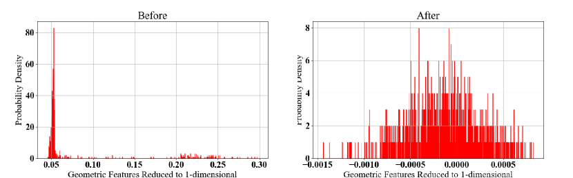
Figure 13: Probability Distribution of Reduced Geometric Features. Left: before the GFF module. Right: after the GFF module.

VI-D Geometry Augmented CDL

As previously discussed in Section III-B, the reference point set for CDL can be selected from LiDAR depth data or from object 3D models. In Table V, we conduct a performance comparison of our approach with these two reference point choices, and we observe enhancements in our methods when employing geometry augmentation techniques.

To provide further clarity, the first method calculates the Chamfer distance by comparing the decoded point set to the input LiDAR-derived point set in a self-supervised fashion. The encoder-decoder structure in this method compels the embedding to acquire a refined depth representation, which fulfills a distinct denoising objective when compared to the previously mentioned GFF module. This depth representation aids in mitigating subtle disturbances but may not effectively address substantial noise that alters the overall shape of an object.

On the other hand, in the second approach, we calculate the CDL by comparing the decoded point set with the point set generated from the 3D model of the corresponding object. In this method, we utilize object models that are not transformed with the ground truth poses. Consequently, this compels the embedding to acquire a pure geometric representation, unaffected by rotation and translation.

It is worth highlighting that the 3D model is only required during the training process for loss computation. In contrast, during inference, our method operates without the necessity of a 3D model. This sets our approach apart from previously discussed RGB-only methods[27, 36, 3]. The object model-augmented CDL outperforms the basic setup, specifically CDL with LiDAR depth, across all metrics (Table V).

VII Conclusion

We have presented DTTDNet as a novel digital-twin localization algorithm to bridge the performance gap for 3D object tracking in mobile applications and with critical requirements of accuracy. At the algorithm level, DTTDNet is a transformer-based 6DoF pose estimator, specifically designed to navigate the complexities introduced by noisy depth data, which is a common issue in mobile AR applications. At the experiment level, we have expanded the scope of our previous work DTTD1[10] by introducing DTTD2, a new RGBD dataset captured using iPhone 14 Pro, whose RGBD camera is of lower quality and cheaper than dedicated depth cameras. Through extensive experiments and ablation analysis, we have examined the effectiveness of our method in being robust to erroneous depth data. Additionally, our research has brought to light new complexities associated with object tracking in dynamic AR environments.

Author Introductions

Zixun Huang is a graduate student researcher in FHL Vive Center at the University of California, Berkeley, who designs algorithms and develops problem-oriented applications to uncover and meet people needs. His research interests include 3D computer vision, multi-modality, and robotics.

Keling Yao holds a Bachelor of Science degree in Data Science and Big Data Technology from the University of Hong Kong, Shenzhen, and visited the University of California, Berkeley as an exchange student in the department of EECS. His research interests include deep learning and robotics with computer vision.

Seth Z. Zhao holds a Master of Science and Bachelor of Arts degree in Electrical Engineering and Computer Science from the University of California, Berkeley. His research interests include Multimodal Deep Learning across Vision, Language, Speech domains, and applications on Autonomous Driving.

Chuanyu Pan holds a Master of Engineering degree in Electrical Engineering and Computer Science from the University of California, Berkeley, and a Bachelor of Science degree in Computer Science from Tsinghua University. His research interests include 3D computer vision and computer graphics.

Tianjian Xu holds a Master of Engineering degree in EECS from the University of California, Berkeley and a Bachelor of Science degree in Computer Science from the University of Southern California. His research interests include computer graphics and mixed reality.

Weiyu Feng holds a Master of Engineering degree in EECS from the University of California, Berkeley and a Bachelor degree in Computer Science from the University of Missouri-Columbia and Beijing Jiaotong University. His research interest includes 3D Vision and Human-Computer Interaction.

Dr. Allen Y. Yang is a Principal Investigator at UC Berkeley and a Co-Founder and CTO of Grafty, Inc. Previously he served as CTO and Acting COO of Atheer Inc. His primary research areas include high-dimensional pattern recognition, computer vision, image processing, and applications in motion segmentation, imagesegmentation, face recognition, and sensor networks.

References

- [1] Gilad Baruch, Zhuoyuan Chen, Afshin Dehghan, Tal Dimry, Yuri Feigin, Peter Fu, Thomas Gebauer, Brandon Joffe, Daniel Kurz, Arik Schwartz, et al. Arkitscenes: A diverse real-world dataset for 3d indoor scene understanding using mobile rgb-d data. arXiv preprint arXiv:2111.08897, 2021.
- [2] Fan Bu, Trinh Le, Xiaoxiao Du, Ram Vasudevan, and Matthew Johnson-Roberson. Pedestrian planar lidar pose (pplp) network for oriented pedestrian detection based on planar lidar and monocular images. IEEE Robotics and Automation Letters, 5(2):1626–1633, 2019.
- [3] Dingding Cai, Janne Heikkilä, and Esa Rahtu. Ove6d: Object viewpoint encoding for depth-based 6d object pose estimation. In Proceedings of the IEEE/CVF Conference on Computer Vision and Pattern Recognition (CVPR), pages 6803–6813, June 2022.
- [4] Berk Calli, Arjun Singh, James Bruce, Aaron Walsman, Kurt Konolige, Siddhartha Srinivasa, Pieter Abbeel, and Aaron M Dollar. Yale-cmu-berkeley dataset for robotic manipulation research. The International Journal of Robotics Research, 36(3):261–268, 2017.
- [5] Berk Calli, Arjun Singh, Aaron Walsman, Siddhartha Srinivasa, Pieter Abbeel, and Aaron M. Dollar. The ycb object and model set: Towards common benchmarks for manipulation research. In 2015 International Conference on Advanced Robotics (ICAR), pages 510–517, 2015.
- [6] Berk Calli, Aaron Walsman, Arjun Singh, Siddhartha Srinivasa, Pieter Abbeel, and Aaron M. Dollar. Benchmarking in manipulation research: Using the yale-cmu-berkeley object and model set. IEEE Robotics & Automation Magazine, 22(3):36–52, 2015.
- [7] Carlos Campos, Richard Elvira, Juan J. G’omez, Jos’e M. M. Montiel, and Juan D. Tard’os. ORB-SLAM3: An accurate open-source library for visual, visual-inertial and multi-map SLAM. IEEE Transactions on Robotics, 37(6):1874–1890, 2021.
- [8] Alexey Dosovitskiy, Lucas Beyer, Alexander Kolesnikov, Dirk Weissenborn, Xiaohua Zhai, Thomas Unterthiner, Mostafa Dehghani, Matthias Minderer, Georg Heigold, Sylvain Gelly, Jakob Uszkoreit, and Neil Houlsby. An image is worth 16x16 words: Transformers for image recognition at scale, 2021.
- [9] Chaojing Duan, Siheng Chen, and Jelena Kovacevic. 3d point cloud denoising via deep neural network based local surface estimation, 2019.
- [10] Weiyu Feng, Seth Z. Zhao, Chuanyu Pan, Adam Chang, Yichen Chen, Zekun Wang, and Allen Y. Yang. Digital twin tracking dataset (dttd): A new rgb+depth 3d dataset for longer-range object tracking applications. In Proceedings of the IEEE/CVF Conference on Computer Vision and Pattern Recognition (CVPR) Workshops, pages 3288–3297, June 2023.
- [11] Bo Gu, Jianxun Liu, Huiyuan Xiong, Tongtong Li, and Yuelong Pan. Ecpc-icp: A 6d vehicle pose estimation method by fusing the roadside lidar point cloud and road feature. Sensors, 21(10):3489, 2021.
- [12] Yong Guo, David Stutz, and Bernt Schiele. Robustifying token attention for vision transformers, 2023.
- [13] Hussein Haggag, Mohammed Hossny, D. Filippidis, Douglas C. Creighton, Saeid Nahavandi, and Vinod Puri. Measuring depth accuracy in rgbd cameras. 2013, 7th International Conference on Signal Processing and Communication Systems (ICSPCS), pages 1–7, 2013.
- [14] Kaiming He, Xinlei Chen, Saining Xie, Yanghao Li, Piotr Dollár, and Ross Girshick. Masked autoencoders are scalable vision learners, 2021.
- [15] Lingzhi He, Hongguang Zhu, Feng Li, Huihui Bai, Runmin Cong, Chunjie Zhang, Chunyu Lin, Meiqin Liu, and Yao Zhao. Towards fast and accurate real-world depth super-resolution: Benchmark dataset and baseline. arXiv preprint arXiv:2104.06174, 2021.
- [16] Yisheng He, Haibin Huang, Haoqiang Fan, Qifeng Chen, and Jian Sun. Ffb6d: A full flow bidirectional fusion network for 6d pose estimation. In IEEE/CVF Conference on Computer Vision and Pattern Recognition (CVPR), June 2021.
- [17] Yisheng He, Wei Sun, Haibin Huang, Jianran Liu, Haoqiang Fan, and Jian Sun. Pvn3d: A deep point-wise 3d keypoints voting network for 6dof pose estimation. In IEEE/CVF Conference on Computer Vision and Pattern Recognition (CVPR), June 2020.
- [18] Yisheng He, Yao Wang, Haoqiang Fan, Jian Sun, and Qifeng Chen. Fs6d: Few-shot 6d pose estimation of novel objects. In Proceedings of the IEEE/CVF Conference on Computer Vision and Pattern Recognition (CVPR), pages 6814–6824, June 2022.
- [19] Pedro Hermosilla, Tobias Ritschel, and Timo Ropinski. Total denoising: Unsupervised learning of 3d point cloud cleaning. In Proceedings of the IEEE/CVF international conference on computer vision, pages 52–60, 2019.
- [20] Stefan Hinterstoisser, Vincent Lepetit, Slobodan Ilic, Stefan Holzer, Gary Bradski, Kurt Konolige, and Nassir Navab. Model based training, detection and pose estimation of texture-less 3d objects in heavily cluttered scenes. In Kyoung Mu Lee, Yasuyuki Matsushita, James M. Rehg, and Zhanyi Hu, editors, Computer Vision – ACCV 2012, pages 548–562, Berlin, Heidelberg, 2013. Springer Berlin Heidelberg.
- [21] Tomáš Hodaň, Pavel Haluza, Štěpán Obdržálek, Jiří Matas, Manolis Lourakis, and Xenophon Zabulis. T-LESS: An RGB-D dataset for 6D pose estimation of texture-less objects. IEEE Winter Conference on Applications of Computer Vision (WACV), 2017.
- [22] Veli Ilci and Charles Toth. High definition 3d map creation using gnss/imu/lidar sensor integration to support autonomous vehicle navigation. Sensors, 20(3):899, 2020.
- [23] Xiaoke Jiang, Donghai Li, Hao Chen, Ye Zheng, Rui Zhao, and Liwei Wu. Uni6d: A unified cnn framework without projection breakdown for 6d pose estimation. In Proceedings of the IEEE/CVF Conference on Computer Vision and Pattern Recognition (CVPR), pages 11174–11184, June 2022.
- [24] Leonid Keselman, John Iselin Woodfill, Anders Grunnet-Jepsen, and Achintya Bhowmik. Intel realsense stereoscopic depth cameras, 2017.
- [25] Wonjae Kim, Bokyung Son, and Ildoo Kim. Vilt: Vision-and-language transformer without convolution or region supervision, 2021.
- [26] Y. Labbe, J. Carpentier, M. Aubry, and J. Sivic. Cosypose: Consistent multi-view multi-object 6d pose estimation. In Proceedings of the European Conference on Computer Vision (ECCV), 2020.
- [27] Yann Labbé, Lucas Manuelli, Arsalan Mousavian, Stephen Tyree, Stan Birchfield, Jonathan Tremblay, Justin Carpentier, Mathieu Aubry, Dieter Fox, and Josef Sivic. Megapose: 6d pose estimation of novel objects via render compare, 2022.
- [28] Bo Li, Tianlei Zhang, and Tian Xia. Vehicle detection from 3d lidar using fully convolutional network. arXiv preprint arXiv:1608.07916, 2016.
- [29] Kejie Li, Jia-Wang Bian, Robert Castle, Philip HS Torr, and Victor Adrian Prisacariu. Mobilebrick: Building lego for 3d reconstruction on mobile devices. In Proceedings of the IEEE/CVF Conference on Computer Vision and Pattern Recognition, pages 4892–4901, 2023.
- [30] Tianjiao Li, Lin Geng Foo, Ping Hu, Xindi Shang, Hossein Rahmani, Zehuan Yuan, and Jun Liu. Token boosting for robust self-supervised visual transformer pre-training, 2023.
- [31] Xingyu Liu, Shun Iwase, and Kris M. Kitani. Stereobj-1m: Large-scale stereo image dataset for 6d object pose estimation. In ICCV, 2021.
- [32] Xingyu Liu, Rico Jonschkowski, Anelia Angelova, and Kurt Konolige. Keypose: Multi-view 3d labeling and keypoint estimation for transparent objects. In 2020 IEEE/CVF Conference on Computer Vision and Pattern Recognition (CVPR 2020), 2020.
- [33] Yuan Liu, Yilin Wen, Sida Peng, Cheng Lin, Xiaoxiao Long, Taku Komura, and Wenping Wang. Gen6d: Generalizable model-free 6-dof object pose estimation from rgb images, 2023.
- [34] Pat Marion, Peter R Florence, Lucas Manuelli, and Russ Tedrake. Label fusion: A pipeline for generating ground truth labels for real rgbd data of cluttered scenes. In 2018 IEEE International Conference on Robotics and Automation (ICRA), pages 3325–3242. IEEE, 2018.
- [35] Ningkai Mo, Wanshui Gan, Naoto Yokoya, and Shifeng Chen. Es6d: A computation efficient and symmetry-aware 6d pose regression framework. In Proceedings of the IEEE/CVF Conference on Computer Vision and Pattern Recognition, pages 6718–6727, 2022.
- [36] Van Nguyen Nguyen, Yinlin Hu, Yang Xiao, Mathieu Salzmann, and Vincent Lepetit. Templates for 3d object pose estimation revisited: Generalization to new objects and robustness to occlusions. In Proceedings of the IEEE/CVF Conference on Computer Vision and Pattern Recognition, pages 6771–6780, 2022.
- [37] Sayak Paul and Pin-Yu Chen. Vision transformers are robust learners, 2021.
- [38] Sida Peng, Yuan Liu, Qixing Huang, Xiaowei Zhou, and Hujun Bao. Pvnet: Pixel-wise voting network for 6dof pose estimation. In CVPR, 2019.
- [39] Ivan Permozer and Tihomir Orehovački. Utilizing apple’s arkit 2.0 for augmented reality application development. In 2019 42nd International Convention on Information and Communication Technology, Electronics and Microelectronics (MIPRO), pages 1629–1634, 2019.
- [40] Charles R. Qi, Hao Su, Kaichun Mo, and Leonidas J. Guibas. Pointnet: Deep learning on point sets for 3d classification and segmentation, 2017.
- [41] Alec Radford, Jong Wook Kim, Chris Hallacy, Aditya Ramesh, Gabriel Goh, Sandhini Agarwal, Girish Sastry, Amanda Askell, Pamela Mishkin, Jack Clark, Gretchen Krueger, and Ilya Sutskever. Learning transferable visual models from natural language supervision, 2021.
- [42] Thomas Schöps, Torsten Sattler, and Marc Pollefeys. Bad slam: Bundle adjusted direct rgb-d slam. In 2019 IEEE/CVF Conference on Computer Vision and Pattern Recognition (CVPR), pages 134–144, 2019.
- [43] Jiaming Sun, Zihao Wang, Siyu Zhang, Xingyi He, Hongcheng Zhao, Guofeng Zhang, and Xiaowei Zhou. OnePose: One-shot object pose estimation without CAD models. CVPR, 2022.
- [44] Asher Trockman and J. Zico Kolter. Mimetic initialization of self-attention layers, 2023.
- [45] Ashish Vaswani, Noam Shazeer, Niki Parmar, Jakob Uszkoreit, Llion Jones, Aidan N. Gomez, Lukasz Kaiser, and Illia Polosukhin. Attention is all you need, 2023.
- [46] Chen Wang, Danfei Xu, Yuke Zhu, Roberto Martín-Martín, Cewu Lu, Li Fei-Fei, and Silvio Savarese. Densefusion: 6d object pose estimation by iterative dense fusion. 2019.
- [47] Kehan Wang, Seth Z. Zhao, David Chan, Avideh Zakhor, and John Canny. Multimodal semantic mismatch detection in social media posts. In Proceedings of IEEE 24th International Workshop on Multimedia Signal Processing (MMSP), 2022.
- [48] Xinshuo Weng and Kris Kitani. Monocular 3d object detection with pseudo-lidar point cloud. In Proceedings of the IEEE/CVF International Conference on Computer Vision Workshops, pages 0–0, 2019.
- [49] Yu Xiang, Tanner Schmidt, Venkatraman Narayanan, and Dieter Fox. Posecnn: A convolutional neural network for 6d object pose estimation in cluttered scenes. 2018.
- [50] Yurong You, Yan Wang, Wei-Lun Chao, Divyansh Garg, Geoff Pleiss, Bharath Hariharan, Mark Campbell, and Kilian Q Weinberger. Pseudo-lidar++: Accurate depth for 3d object detection in autonomous driving. arXiv preprint arXiv:1906.06310, 2019.
- [51] Sergey Zakharov, Ivan Shugurov, and Slobodan Ilic. Dpod: 6d pose object detector and refiner. pages 1941–1950, 10 2019.
- [52] Haojie Zhao, Junsong Chen, Lijun Wang, and Huchuan Lu. Arkittrack: A new diverse dataset for tracking using mobile rgb-d data. In Proceedings of the IEEE/CVF Conference on Computer Vision and Pattern Recognition, pages 5126–5135, 2023.
- [53] Kun Zhou, Hui Yu, Wayne Xin Zhao, and Ji-Rong Wen. Filter-enhanced MLP is all you need for sequential recommendation. In Proceedings of the ACM Web Conference 2022. ACM, apr 2022.