A Novel Stochastic Interacting Particle-Field Algorithm for 3D Parabolic-Parabolic Keller-Segel Chemotaxis System

Abstract

We introduce an efficient stochastic interacting particle-field (SIPF) algorithm with no history dependence for computing aggregation patterns and near singular solutions of parabolic-parabolic Keller-Segel (KS) chemotaxis system in three space dimensions (3D). The KS solutions are approximated as empirical measures of particles coupled with a smoother field (concentration of chemo-attractant) variable computed by the spectral method. Instead of using heat kernels causing history dependence and high memory cost, we leverage the implicit Euler discretization to derive a one-step recursion in time for stochastic particle positions and the field variable based on the explicit Green’s function of an elliptic operator of the form Laplacian minus a positive constant. In numerical experiments, we observe that the resulting SIPF algorithm is convergent and self-adaptive to the high gradient part of solutions. Despite the lack of analytical knowledge (e.g. a self-similar ansatz) of the blowup, the SIPF algorithm provides a low-cost approach to study the emergence of finite time blowup in 3D by only dozens of Fourier modes and through varying the amount of initial mass and tracking the evolution of the field variable. Notably, the algorithm can handle at ease multi-modal initial data and the subsequent complex evolution involving the merging of particle clusters and formation of a finite time singularity.

AMS subject classification: 35K57, 92C17, 65C35, 65M70, 65M75.
Keywords: fully parabolic Keller-Segel system, interacting particle-field approximation, singularity detection, critical mass.

1 Introduction

Chemotaxis partial differential equations (PDEs) were introduced by Keller and Segel (KS [15]) to describe the aggregation of the slime mold amoeba Dictyostelium discoideum due to an attractive chemical substance. Related random walk model by Patlak was known earlier [24], see [29] for an analysis of basic taxis behaviors (aggregation, blowup, and collapse) based on reinforced random walks. We consider the parabolic-parabolic (fully parabolic) KS system of the form:

$$\rho_{t} =\nabla\cdot(\mu\,\nabla\rho-\chi\,\rho\,\nabla c),$$

$$\epsilon\,c_{t} =\Delta\,c-k^{2}\,c+\rho,$$ (1)

where $\chi,\mu$ ($\epsilon,k$) are positive (non-negative) constants. The model is called elliptic if $\epsilon=0$ (when $c$ evolves rapidly to a local equilibrium), and parabolic if $\epsilon>0$. The $\rho$ is the density of active particles (bacteria), and $c$ is the concentration of chemo-attractant (e.g. food). See detail discussion in Section 2

The KS systems (1) have been studied for several decades, with various cases and dimensions explored. For the parabolic-elliptic case with $k=0$ and $\epsilon=0$, Herrero et al [11] investigated the 3D case and found the existence of self-similar radial blowup, while such a blowup does not occur in 2D. An overview of blow-up phenomena, particularly in 2D, can be found in the book by Perthame [25]. In [8], Giga et al. further explored the parabolic-elliptic case with $k=0$ and introduced the concept of type I blowup, denoted by $y_{t}=y^{2}$. They demonstrated that when the spatial dimension $d>3$, all type-I radial blowup is self-similar. More recently, Souplet and Winkler [27] provided a detailed profile of the 3D parabolic-elliptic self-similar blowup satisfying the inequality $u(x,t)\leq C(T-t+|x|^{2})^{-1}$, where $C$ is a constant.

The fully parabolic case, i.e. system (1) with $\epsilon\not=0$, has also been extensively studied. In the 2D fully parabolic case, Herrero and Velázquez [12] demonstrated the existence of self-similar Dirac-delta type blow-up in the 2D fully parabolic case for $k\not=0$; while Calvez and Corrias [1] and Mizoguchi [23] showed that under mild assumptions on the initial conditions, a global weak solution exists for mass $M_{0}<8\pi$. In contrast, for super-critical mass, the system blows up in finite time under the smallness assumption of the second moment. Further work by Lemarié-Rieusset [17] proved global existence and stability in $\mathbb{R}^{n}$ with small initial data in the critical Morrey space. When $k=0$, Takeuchi [30] demonstrated the existence of a global strong solution on $\mathbb{R}^{n}$ provided that the initial data is small in the homogeneous Besov space, which is scaling invariant.

Several notable numerical methods have been developed for KS systems to date. Chertock et al. [5] developed a finite-volume method for a class of chemotaxis models and a closely related haptotaxis model. This approach allows for accurate and efficient simulations of chemotaxis phenomena. Shen et al. [26] proposed an energy dissipation and bound preserving scheme that is not restricted to specific spatial discretization. The bound preserving property is achieved through modification of the system. In a related work, Hillen and Othmer [13] assumed a saturation concentration $M_{0}$ for the bacteria, such that if $\rho>M$, there is no chemo-attractant contribution. Under this assumption, the system does not blow up and still exhibits spiky solutions. Chen et al. [3] developed a fully-discrete finite element method (FEM) scheme for the 2D classical parabolic-elliptic Keller-Segel system, following the approach of Shen et al. [26]. They showed that the proposed scheme will blow up in a finite time, under assumptions similar to those in the continuous blow-up scenarios. In the classic setting, Liu and Wang [18] reformulated the equation using the Le Châtelier Principle to attain a positive-preserving scheme. It is worth noting that all the aforementioned numerical methods are tailored for 2D cases.

Besides the Eulerian discretization methods above, there have been theoretical developments in the Lagrangian framework for the KS system (1) and related equations. Stevens [28] derived an $N$-particle system with convergence in the fully parabolic case. Additionally, Havskovéč and Ševčovič [9] developed a convergent regularized particle system for the 2D parabolic elliptic case. Havskovéč and Markowich [10] demonstrated convergence in the BBGKY hierarchy modulo a gap due to the lack of uniqueness of the Boltzmann hierarchy. This gap was addressed by Mischler and Mouhot [22] who studied the propagation of chaos and mean-field limits for systems of indistinguishable particles undergoing collisions. Craig and Bertozzi [6] proved the convergence of a blob method for the related aggregation equation. In the study of the KS system, Liu et al. [20] and [19] developed a random particle blob method with a mollified kernel for the parabolic-elliptic case. They demonstrated convergence when the limiting (macroscopic mean field) equation admits a global weak solution. As noted by Mischler and Mouhot [22], the success of this analysis strongly relies on detailed knowledge of the nonlinear mean field equation, rather than the details of the underlying many-particle Markov process. A particle computation based on [9] for the 2D advective parabolic-elliptic KS system, i.e. (1) with $\epsilon=0$ and an additional passive flow, was conducted in [16]. A deep learning study for chemotaxis aggregation in 3D laminar and chaotic flows based on a kernel regularization technique of a particle method by the present authors is in [31].

Most existing particle-field algorithms for KS equations are deterministic, assuming that the underlying particle systems are well-mixed. In this paper, we propose a novel stochastic interacting particle-field (SIPF) algorithm for the fully parabolic KS system (1). Our method takes into account the coupled stochastic particle evolution (density $\rho$) and the accompanying field (concentration $c$) in the system and allows for a self-adaptive simulation of focusing and potentially singular behavior.In the SIPF algorithm, we represent the active particle density $\rho$ by empirical particles and the concentration field $c$ is discretized by a spectral method instead of a finite difference method [7]. This is possible since the field $c$ is smoother than density $\rho$. We demonstrate the effectiveness of our method through numerical experiments in three space dimensions (3D), which have not been systematically computed and benchmarked to the best of our knowledge.

It is worth noting that the pseudo-spectral methods were employed to compute the nearly singular solutions of the 3D Euler equations [14]. Subsequently, the finite-time blowup of the 3D axisymmetric Euler equations was computed using the adaptive moving mesh method [21]. These methods represent the cutting edge in the computation of nearly singular solutions of the 3D Euler equations. Nevertheless, we also point out that the implementation of pseudo-spectral methods for 3D problems demands substantial computational resources, while the adaptive moving mesh method requires sophisticated design and advanced programming skills.

It is also worth noting that the Lagrangian algorithms in computation of parabolic-elliptic KS system, for instance [9], cannot be directly generalized to fully parabolic cases. Those algorithms rely on that the field $c$ at time $t$ can be accessed by particle density $\rho$ at the same instant. Hence one only needs to update the particle density locally in time. A direct generalization to the fully parabolic case will require historical particle density $\rho$ from the starting time of the algorithm. An example and related convergence analyses can be found in [2]. However from computational perspective, the volume of such historical data increases in time and becomes a costly burden on memory and flops. In contrast, our SIPF algorithm computes particle and field once per time step without involving a long past history so the computational cost does not grow in time.

The goal of this paper is to introduce a novel stochastic interacting particle-field algorithm (SIPF) for the fully parabolic KS system. Though we verify the convergence of SIPF algorithm numerically, the theoretical study will be left for a future work.

The rest of the paper is organized as follows. In Section 2, we briefly review the blow-up behavior in the fully parabolic KS models under critical mass conditions and the Lagrangian formulations in the computation of KS models. In Section 3, we present our SIPF algorithms for solving the fully parabolic KS system by simplifying a theoretically equivalent yet computationally undesirable method with history dependent parabolic kernel functions (a naive extension of particle method in the parabolic-elliptic case) into efficient recursions. In Section 4, we show numerical results to demonstrate the performance of our method for 3D KS chemotaxis systems. Concluding remarks are given in section 5.

2 Parabolic-Parabolic KS System

In this section, we list some theoretical analyses of singular behaviors and related computational methods for Keller Segel (KS) models in both parabolic elliptic cases and parabolic parabolic (fully parabolic) cases. To begin, we recall the KS model:

$$\rho_{t} =\nabla\cdot(\mu\,\nabla\rho-\chi\,\rho\,\nabla c),$$ (2)

$$\epsilon c_{t} =\Delta\,c-k^{2}\,c+\rho,$$ (3)

$$x\in \Omega\subseteq\mathbb{R}^{d},\quad t\in[0,T].$$ (4)

The first equation (2) of $\rho$ models the evolution of the density of active particles (bacteria). The bacteria diffuse with mobility $\mu$ and drift in the direction of $\nabla c$ with velocity $\chi\nabla c$, where $\chi$ is called chemo-sensitivity. The second equation (3) of $c$ models the evolution of the concentration of chemo-attractant (e.g. food). The increment of $c$ is proportion to $\rho$, which indicates the aggregation (attraction) between active particles. Another important physical parameter is $\epsilon$ in Eq.(3), which models the time scale of the chemotaxis. When $\epsilon\not=0$, it is referred to as parabolic parabolic Keller Segel systems. For $\epsilon=0$ the system is reduced to the parabolic-elliptic case, which models the chemical attractant released by the active particle instantly turns to equilibrium.

2.1 From Critical Collapse to Coexistence of Blow-up and Global Smooth Solutions

Well-known KS dichotomy (critical collapse) states that $8\pi$ is the critical mass for the simplest two-dimensional parabolic-elliptic KS system in $\Omega=\mathbb{R}^{2}$, namely (1) with $\epsilon=k=0$,

$$\rho_{t} =\nabla\cdot(\nabla\rho-\rho\,\nabla c),$$

$$\Delta\,c =-\rho,$$ (5)

so that

1. If $M_{0}<8\pi$, the system has a global smooth solution.

2. If $M_{0}>8\pi$, the system blows up in finite time in the sense of $|\cdot|_{\infty}$ norm.

It can be seen from the classical variance identity for system (5), [25], that,

$$\frac{d}{dt}\int_{x\in\mathbb{R}^{2}}|x|^{2}\,\rho(x)\,dx=\frac{M}{2\pi}(8\pi-M).$$ (6)

Then the solution of (5) exhibits a quantized concentration of mass at origin, a $\delta$ type blow-up.

For system (5) on $\mathbb{R}^{d}$ ($d\geq 3$), the identity (6) does not apply and the KS evolution is not as clear cut. Nonetheless, the coexistence of blow-up and global smooth solutions remains depending on the size of the initial data. In addition, there exists the blow-up profile that is different from $\delta$ type blowup. For example, it is shown in [11] that in 3D fully parabolic systems, there exist radial, positive, backward self-similar solutions of the form,

$$\rho(x,t)=\frac{V(x/\sqrt{T-t})}{T-t},\quad\quad 0<t<T,$$ (7)

where the radially decreasing profile function $V$ satisfies $\lim_{y\to\infty}y^{2}V(y)=L\in\mathbb{R}^{+}$.

Later in a more refined result by [27], the blowup is said to be type I if

$$0<\limsup_{t\to T}\,(T-t)\,\|\rho\|_{\infty}\,<\infty.$$ (8)

Then for radial initial data in $L^{1}(\mathbb{R}^{3})$, if a blowup is type I, $\exists\,C>0$ such that

$$\rho(x,t)\leq C(T-t+|x|^{2})^{-1},\quad 0<|x|\leq R,\quad 0<t<T.$$ (9)

On the other side of the dichotomy, it is shown in [30], that the global strong solution exists in the fully parabolic system (1) for small initial data.

The analyses are unknown for the blowup behavior of the KS system on $\mathbb{R}^{3}$ from a non-radial initial value to our best knowledge. One must resort to numerical computation to investigate the possible singular behavior which will be discussed in section 4.3.

2.2 Lagrangian formulations

As a fundamental step of deriving the algorithms, we introduce the Lagrangian formulation of active particle density $\rho$ in the KS system (1) and start with the elliptic system with $\epsilon=k=0$, namely (5) in general $d$ dimension. From $\Delta c=-\rho$ and the Green’s function of Laplacian operator in $R^{d}$, we know,

$$c(x,t)=\left\{\begin{array}[]{l}-\frac{1}{2\pi}\int\ln|x-y|\,\rho(y,t),\quad d=2\\ C_{d}\int\frac{1}{|x-y|^{d-2}}\,\rho(y,t)\,dy,\quad d\geq 3\end{array}\right.,$$ (12)

where $C_{d}=\frac{\Gamma(d/2+1)}{d(d-2)\pi^{d/2}}$. So the convection term in (2) turns to,

$$\nabla c(x)=-\frac{\Gamma(d/2)}{2\pi^{d/2}}\int\frac{x-y}{|x-y|^{d}}\,\rho(y,t)\,dy.$$ (13)

Now we arrive at the interactive stochastic differential equation system of $P$ particles, $\{X^{p}_{t}\}_{p=1:P}$,

$$dX^{p}_{t}=-\chi\frac{M}{P}\sum_{q\not=p}\frac{\Gamma(d/2)}{2\pi^{d/2}}\frac{X^{p}_{t}-X^{q}_{t}}{|X^{p}_{t}-X^{q}_{t}|^{d}}+\sqrt{2\mu}\,dW^{p}_{t},\quad p=1,\cdots,P,$$ (14)

where $W^{p}_{t}$ denotes independent identically distributed standard Brownian motions. In [22], it is shown with mild regularity condition, when $P\to\infty$, the distribution of empirical particles $\{X^{p}_{t}\}_{p=1:P}$ converges to $\rho$ in the continuous PDE system (2). Several novel numerical methods have been developed or implemented to study the singularity behavior in the parabolic elliptic Keller Segel systems, see [19, 9, 31].

In the fully parabolic case ($\epsilon\not=0$), the solution of chemical concentration $c$ comes from solving a parabolic equation, which is non longer Markovian as one in (14). At time $t>0$, solution of $\rho$ in $[0,t]$ has to be involved in the representation of $c$, namely,

$$c(\cdot,t)=e^{-k^{2}t}e^{t\Delta}c(\cdot,0)+\int_{0}^{t}e^{k^{2}(s-t)}e^{(t-s)\Delta}\,\rho(\cdot,s)\,ds,$$ (15)

where the heat semigroup operator $e^{t\Delta}$ is defined by

$$(e^{t\Delta}f)(x,t):=\int\frac{e^{-|x-y|^{2}/(4t)}}{(4\pi t)^{d/2}}\,f(y)\,dy.$$ (16)

Similar to (14), the empirical particle system converging to density $\rho$ reads:

$$dX^{p}=\,{\chi}\nabla_{X}\,c(X^{p}_{t},t)\,dt+\sqrt{2\,\mu}\,dW^{p},\;\;p=1,\cdots,P,$$ (17)

and $W^{p}$’s are independent Brownian motions in $\mathbb{R}^{d}$. Due to the historic path dependent in the solution of $c$ in (15), direct computation of drift $\nabla_{X}\,c(X^{p}_{t},t)$ in (17) will lead to significant memory cost, which increases w.r.t. computational time $T$. To our best knowledge, a memory-less algorithm to compute the fully parabolic KS system has not been developed. We will present one in the following section.

3 SIPF Algorithms for Parabolic-Parabolic KS

In this section, we present the SIPF algorithm for solving the fully parabolic KS models. Since we are interested in the spatially localized aggregation behavior as discussed in Sec 2.1, it is viable that we restrict the system (2) and (3) in a large domain $\Omega=[-L/2,L/2]^{d}$ and assume Dirichlet boundary condition for particle density $\rho$ and Neumann boundary condition for chemical concentration $c$.

As a discrete algorithm, we assume the temporal domain $[0,T]$ is partitioned by $\{t_{n}\}_{n=0:n_{T}}$ with $t_{0}=0$ and $t_{n_{T}}=T$. We approximate the density $\rho$ by particles, i.e.

$$\rho_{t}\approx{\frac{M_{0}}{P}}\,\sum_{j=1}^{P}\delta(x-X^{p}_{t}),\;\;P\gg 1,$$ (18)

where $M_{0}$ is the conserved total mass (integral of $\rho$). For chemical concentration $c$, we approximate by Fourier basis, namely, $c(\textbf{x},t)$ has an series representation

$$\sum_{j,m,l\in\mathcal{H}}\,\alpha_{t;j,m,l}\,\exp(i2\pi j\,x_{1}/L)\exp(i2\pi m\,x_{2}/L)\exp(i2\pi l\,x_{3}/L),$$ (19)

where $\mathcal{H}$ denotes index set

$$\{(j,m,l)\in\mathbb{N}^{3}:|j|,|m|,|l|\leq\frac{H}{2}\},$$ (20)

and $i=\sqrt{-1}$.

Then at $t_{0}=0$, we generate $P$ empirical samples $\{X^{p}_{0}\}_{p=1:P}$ according to the initial condition of $\rho_{0}$ and set up $\alpha_{0;j,m,l}$ by the Fourier series of $c_{0}$.

For ease of presenting our algorithm, with a slight abuse of notation, we use $\rho_{n}={\frac{M_{0}}{P}}\,\sum_{p=1}^{P}\delta(x-X^{p}_{n})$, and

$$c_{n}=\sum_{j,m,l\in\mathcal{H}}\,\alpha_{n;j,m,l}\,\exp(i2\pi j\,x_{1}/L)\exp(i2\pi m\,x_{2}/L)\exp(i2\pi l\,x_{3}/L)$$

to represent density $\rho$ and chemical concentration $c$ at time $t_{n}$.

Considering time stepping system (1) from $t_{n}$ to $t_{n+1}$, with $\rho_{n}$ and $c_{n-1}$ known, our algorithm, inspired by the operator splitting technique, consists of two sub-steps: updating chemical concentration $c$ and updating organism density $\rho$.

Updating chemical concentration $c$

Let $\delta t=t_{n+1}-t_{n}>0$ be the time step. We discretize the $c$ equation of (1) in time by an implicit Euler scheme:

$$\epsilon\,(c_{n}-c_{n-1})/\delta t=(\Delta-k^{2})\,c_{n}+\rho_{n}.$$ (21)

From (21), we obtain the explicit formula for $c_{n}$ as:

$$(\Delta-k^{2}-\epsilon/\delta t)\,c_{n}=-\epsilon\,c_{n-1}/\delta t-\rho_{n}.$$ (22)

It follows that:

$$c_{n}=c(\textbf{x},t_{n}) =-\mathcal{K}_{\epsilon,\delta t}\ast(\epsilon\,c_{n-1}/\delta t+\rho_{n})=-\mathcal{K}_{\epsilon,\delta t}\ast(\epsilon\,c(\textbf{x},t_{n-1})/\delta t+\rho(x,t_{n}))$$ (23)

where $\ast$ is spatial convolution operator, and $\mathcal{K}_{\epsilon,\delta t}$ is the Green’s function of the operator $\Delta-k^{2}-\epsilon/\delta t$. In case of $\mathbb{R}^{3}$, the Green’s function $\mathcal{K}_{\epsilon,\delta t}$ reads as follows

$$\mathcal{K}_{\epsilon,\delta t}=\mathcal{K}_{\epsilon,\delta t}(\textbf{x})=-\frac{\exp\{-\beta|\textbf{x}|\}}{4\pi|\textbf{x}|}.\quad\beta^{2}=k^{2}+\epsilon/\delta t,$$ (24)

The Green’s function admits a closed form Fourier transform,

$$\mathcal{F}\mathcal{K}_{\epsilon,\delta t}(\omega)=-\frac{1}{|\omega|^{2}+\beta^{2}}.$$ (25)

For the term $-\mathcal{K}_{\epsilon,\delta t}\ast c_{n-1}$ in (23), by Eq.(25) it is equivalent to modify Fourier coefficients $\alpha_{j,m,l}$ to $\alpha_{j,m,l}/(4\pi^{2}j^{2}/L^{2}+4\pi^{2}m^{2}/L^{2}+4\pi^{2}l^{2}/L^{2}+\beta^{2})$.

For the second term $\mathcal{K}_{\epsilon,\delta t}\ast\rho$, we first approximate $\mathcal{K}_{\epsilon,\delta t}$ with $\cos$ series expansion, then according to the particle representation of $\rho$ in (18),

$$(\mathcal{K}_{\epsilon,\delta t}\ast\rho)_{j,m,l}\approx\frac{M_{0}}{P}\sum_{p=1}^{P}\frac{\exp(-2\pi jX^{p}_{n,1}/L-2\pi mX^{p}_{n,2}/L-2\pi lX^{p}_{n,l}/L)(-1)^{j+m+l}}{4\pi^{2}j^{2}/L^{2}+4\pi^{2}m^{2}/L^{2}+4\pi^{2}l^{2}/L^{2}+\beta^{2}}.$$ (26)

Finally, we summarize the one-step update of Fourier coefficients of chemical concentration $c$ in Alg.1.

Data: Distribution $\rho_{n}$ represented by empirical samples $X_{n}$ , initial concentration $c_{n-1}$ represented by Fourier coefficients $\alpha_{n-1}$;

for $(j,m,l)\in\mathcal{H}$ do

       $\alpha_{n;j,m,l}\leftarrow\frac{\epsilon\alpha_{n-1;j,m,l}}{\delta t(4\pi^{2}j^{2}/L^{2}+4\pi^{2}m^{2}/L^{2}+4\pi^{2}l^{2}/L^{2}+\beta^{2})}$

       $F_{j,m,l}\leftarrow 0$.

       for $p=1$ to P do

             $F_{j,m,l}\leftarrow F_{j,m,l}+\exp(-2\pi jX^{p}_{n;1}/L-2\pi mX^{p}_{n;2}/L-2\pi lX^{p}_{n;3}/L)$

       end for

      $F_{j,m,l}\leftarrow F_{j,m,l}\frac{(-1)^{j+m+l}}{4\pi^{2}j^{2}/L^{2}+4\pi^{2}m^{2}/L^{2}+4\pi^{2}l^{2}/L^{2}+\beta^{2}}*\frac{M}{P}$

end for

$\alpha_{n}\leftarrow\alpha_{n}-F$

Result: Updated chemical concentration field from input $c_{n-1}$ to $c_{n}$ via $\alpha_{n}$.

Algorithm 1 One step update of chemical concentration in SIPF

Updating density of active particles $\rho$

In the one-step update of density $\rho_{n}$ represented by particles $\{X_{n}^{p}\}_{p=1:P}$, we apply Euler-Maruyama scheme to solve the SDE (17):

$$X^{p}_{n+1}=X^{p}_{n}+\chi\nabla_{\textbf{x}}c(X^{p}_{n},t_{n})\delta t+\sqrt{2\,\mu\,\delta t}\,N^{p}_{n},$$ (27)

where $N^{p}_{n}$’s are i.i.d. standard normal distributions with respect to the Brownian paths in the SDE formulation (17). For $n>1$, substituting (23) in (27) gives:

$$X^{p}_{n+1}=X^{p}_{n}-\chi\nabla_{\textbf{x}}\mathcal{K}_{\epsilon,\delta t}\ast(\epsilon\,c_{n-1}(\textbf{x})/\delta t+\rho_{n}(\textbf{x}))|_{\textbf{x}=X^{p}_{n}}\delta t+\sqrt{2\,\mu\,\delta t}\,N^{p}_{n},$$ (28)

from which $\rho_{n+1}(\textbf{x})$ is constructed via (18).

In such particle formulation, the computation of spacial convolution is slightly different from one in the update of $c$, namely (23).

For $\nabla_{\textbf{x}}\mathcal{K}_{\epsilon,\delta t}\ast\,c_{n-1}(X^{p}_{n})$, to avoid the singular points of $\nabla_{\textbf{x}}\mathcal{K}_{\epsilon,\delta t}$, we evaluate the integral with the quadrature points that are away from $0$. Precisely, denote the standard quadrature point in $\Omega$ with

$$x_{j,m,l}=(j\,L/H,m\,L/H,j\,L/H),$$ (29)

where $j$, $m$, $l$ are integers ranging from $-H/2$ to $H/2-1$. When computing the integral $\nabla_{\textbf{x}}\mathcal{K}_{\epsilon,\delta t}\ast\,c_{n-1}(X^{p}_{n})$, we evaluate $\nabla_{\textbf{x}}\mathcal{K}_{\epsilon,\delta t}$ at $\{X^{p}_{n}+\bar{X}^{p}_{n}-x_{j,m,l}\}_{j,m,l}$ where a small spatial shift $\bar{X}^{p}_{n}=\frac{H}{2L}+\lfloor\frac{X^{p}_{n}}{H/L}\rfloor\frac{H}{L}-X^{p}$ and $c$ at $\{x_{j,m,l}-\bar{X}^{p}_{n}\}_{j,m,l}$ correspondingly. The latter one is computed by inverse Fourier transform of shifted coefficients, with $\alpha_{j,m,l}$ modified to $\alpha_{j,m,l}\exp(-i2\pi j\bar{X}^{p}_{n;1}/L-i2\pi m\bar{X}^{p}_{n;2}/L-i2\pi l\bar{X}^{p}_{n;3}/L)$ where $(\bar{X}^{p}_{n;i})$ denotes the $i$-th component of $\bar{X}^{p}_{n}$.

The term $\nabla_{\textbf{x}}\mathcal{K}_{\epsilon,\delta t}\ast\,\rho(X^{p}_{n},t_{n})$ is straightforward thanks to the particle representation of $\rho(X^{p}_{n},t_{n})$ in (18):

$$\nabla_{\textbf{x}}\mathcal{K}_{\epsilon,\delta t}\ast\,\rho_{n}(X^{p}_{n})=\int\mathcal{K}_{\epsilon,\delta t}(X^{p}_{n}-y)\rho(y)\approx\sum_{q=1,q\not=p}^{P}\frac{M}{P}\mathcal{K}_{\epsilon,\delta t}(X^{p}_{n}-X^{q}_{n}).$$ (30)

We summarize the one-step update (for $n>1$) of density in SIPF as in Alg.2.

Data: Distribution $\rho_{n}$ represented by empirical samples $X_{n}$, input: concentration $c_{n-1}$ represented by Fourier coefficients $\alpha_{n-1}$;

for $p=1$ to P do

       $X_{n+1}^{p}\leftarrow X_{n+1}^{p}+\sqrt{2\mu\delta t}N$ where $N$ is a random generated standard normal distribution.

       for $q=1$ to P do

             $X_{n+1}^{p}\leftarrow X_{n+1}^{p}-\frac{\chi M\delta t}{P}\mathcal{K}_{\epsilon,\delta t}(X^{p}_{n}-X^{q}_{n})$

       end for

      $\bar{X}^{p}_{n}\leftarrow\frac{H}{2L}+\lceil\frac{X^{p}_{n}}{H/L}\rceil\frac{H}{L}-X^{p}$

      

      for $(j,m,l)\in\mathcal{H}$ do

             $F_{j,m,l}\leftarrow\nabla_{\textbf{x}}\mathcal{K}_{\epsilon,\delta t}(X^{p}_{n}+\bar{X}_{n}^{p}-x_{j,m,l}),\;\;$ $x_{j,m,l}$ from Eq. (29)

             $G_{j,m,l}\leftarrow\alpha_{j,m,l}\exp(-i2\pi j\bar{X}^{p}_{n;1}/L-i2\pi m\bar{X}^{p}_{n;2}/L-i2\pi l\bar{X}^{p}_{n;3}/L)$

       end for

      

      $\check{G}=iFFT(G)$

      

      $X_{n+1}^{p}\leftarrow X_{n+1}^{p}-\epsilon\chi(F,\check{G})\frac{L^{3}}{H^{3}}$, where $(\cdot,\cdot)\frac{L^{3}}{H^{3}}$ denote an inner product corresponding to $L^{2}(\Omega)$ quadrature.

end for

Result: Output $\rho_{n+1}$ represented by updated $X_{n+1}.$

Algorithm 2 One step update of density in SIPF

Combining (23) and (28), we conclude that the recursion from $(\{X^{p}_{n}\}_{p=1:P},\rho_{n}(\textbf{x}),c_{n-1}(\textbf{x}))$ to $(\{X^{p}_{n+1}\}_{p=1:P},\rho_{n+1}(\textbf{x}),c_{n}(\textbf{x}))$ is complete. We summarize the SIPF method in the following Algorithm 3.

Data: Initial distribution $\rho_{0}$, initial concentration $c_{0}$;

Generate $P$ i.i.d samples following distribution $\rho_{0}$, $X^{1},X^{2},\cdots X^{P}$.

for $p\leftarrow 1$ to $P$ do

      Compute $X^{p}_{1}$ by (27), with $c_{-1}=c_{0}$

end for

Compute $c_{1}$ by Alg.1 with $c_{0}$ and $\rho_{1}=\sum_{p=1}^{P}\frac{M}{P}\delta_{X^{p}_{1}}$.

for step $n\leftarrow 2$ to $N=T/\delta t$  do

      Compute $X_{n}$ by Alg.2 with $\rho_{n-1}$ and $c_{n-2}$

      Compute $c_{n}$ by Alg.1 with $c_{n-1}$ and $\rho_{n}=\sum_{p=1}^{P}\frac{M}{P}\delta_{X^{p}_{n}}$.

end for

Algorithm 3 Stochastic Interacting Particle-Field Method

4 Numerical Experiments

4.1 Aggregation Behaviors

To illustrate the functionality of the algorithm, we start with two examples. In both cases, the initial distribution $\rho_{0}$ is assumed to be a uniform distribution over a ball centered at $\begin{bmatrix}0\\ 0\\ 0\end{bmatrix}$ with radius $1$, see Fig.1(a). Also in both cases, we assume the following model parameters,

$$\mu=\chi=1,\quad\epsilon=10^{-4}\text{ and }k=10^{-1}.$$ (31)

for the fully parabolic Keller Segel model (1). The choice (31) is made so that the model exhibits comparable behavior as the corresponding parabolic-elliptic KS system whose blow-up behavior is known. For the first example, the total mass is chosen to be $M_{0}=20$, while for the second, the mass is $M_{0}=80$.

In the numerical computation of both examples, we use $H=24$ Fourier basis in each spatial dimension to discretize chemical concentration $c$ and use $P=10000$ particles to represent approximated distribution $\rho$. The computational domain is in the domain $\Omega=[-L/2,L/2]^{3}$ where $L=8$. We then compute the evolution of $c$ and $\rho$ via Alg.3 with $\delta t=10^{-4}$ up to $T=0.1$.

(a) $T=0$

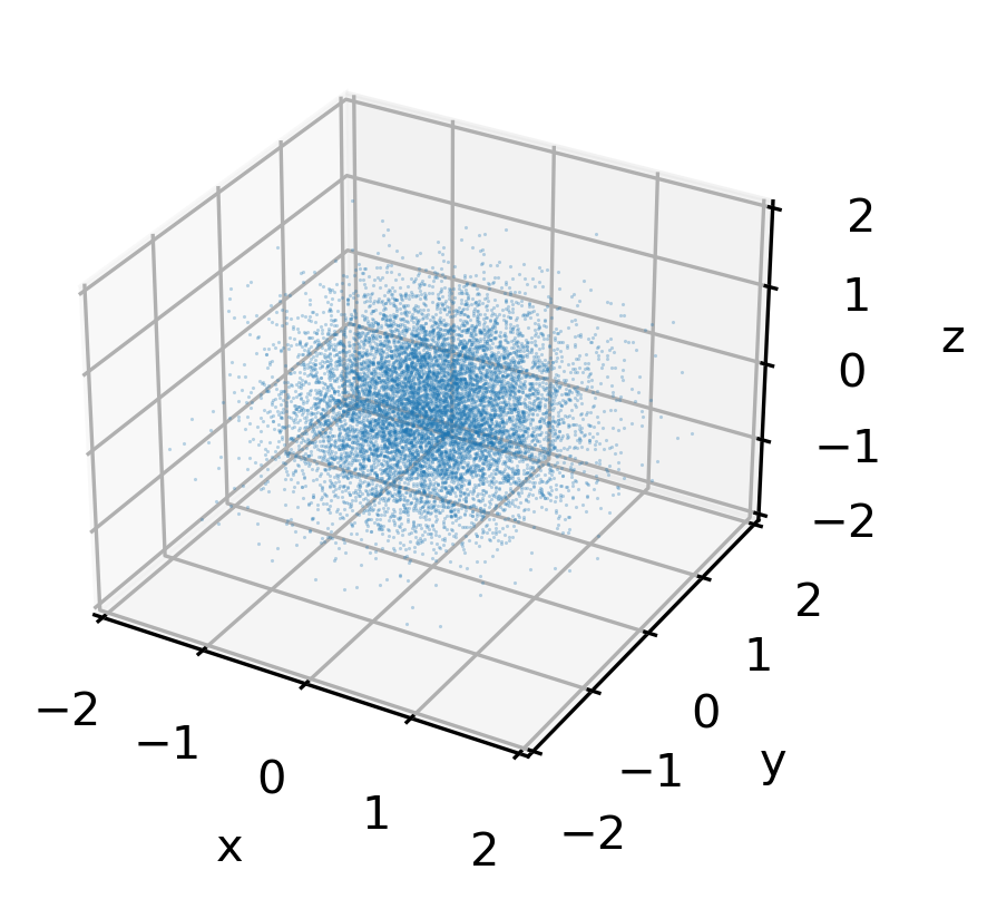
(b) $T=0.1$, $M_{0}=20$

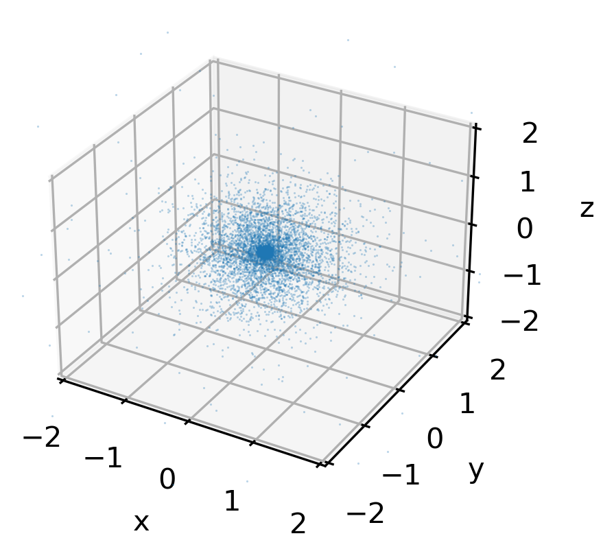
(c) $T=0.1$, $M_{0}=80$

Figure 1: Density $\rho$ approximated by empirical distribution at $T=0.1$: the mass effect on focusing.

In Fig.1, we plot the distribution $\rho$ by empirical samples, at the starting time $T=0$ and final computation time $T=0.1$. In Fig.1(b), we can see the diffusive behaviors compared with the initial distribution shown in Fig.1(a). While in Fig.1(c), we increase the total mass from $M_{0}=20$ to $M_{0}=50$, we can see particles become concentrated at the origin, which indicates the possible blow-up of the continuous system.

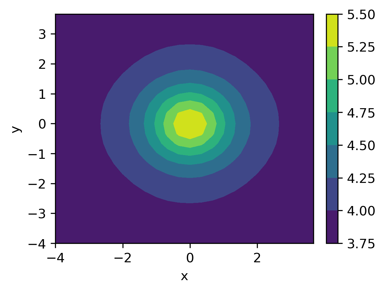
(a) $M_{0}=20$

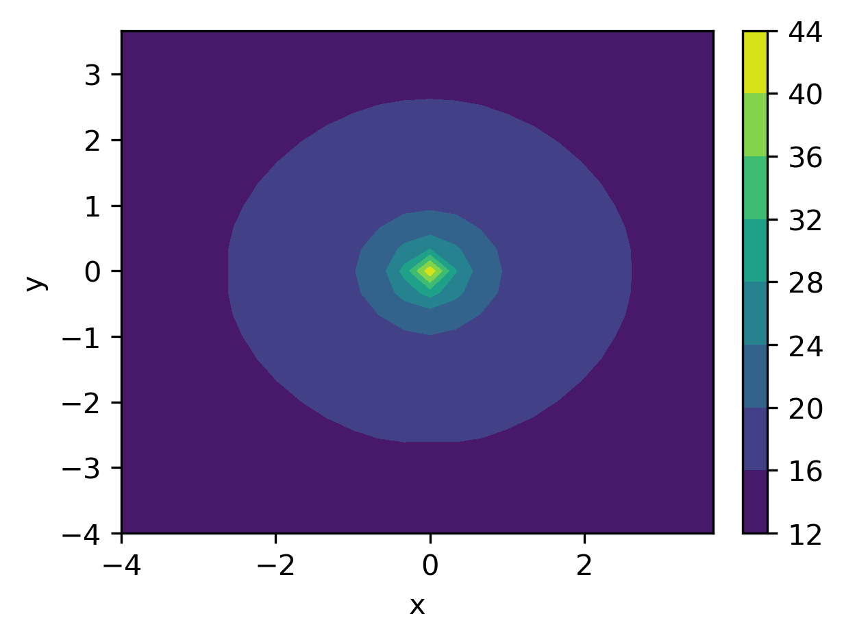
(b) $M_{0}=80$

Figure 2: Chemical concentration $c$ at final time $T=0.1$, sliced at $z=0$.

In Fig.2, we present the chemical concentration $c$ at final time $T=0.1$ and third component $z=0$ for various $M_{0}$. By comparing the subfigures, we can see that in the large total mass case, $c$ exhibits a sharp profile at the origin due to the near singular behavior of $\rho$ towards a possible blow-up.

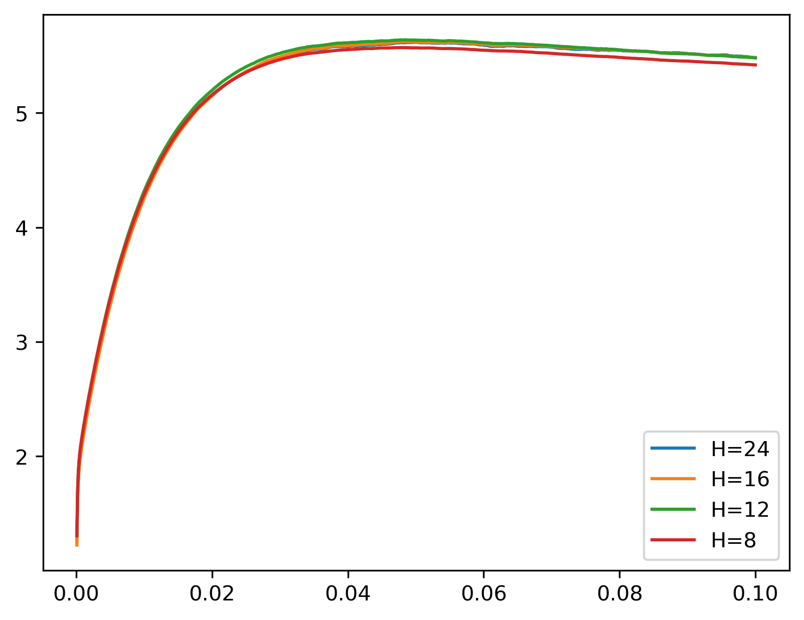
(a) $M_{0}=20$

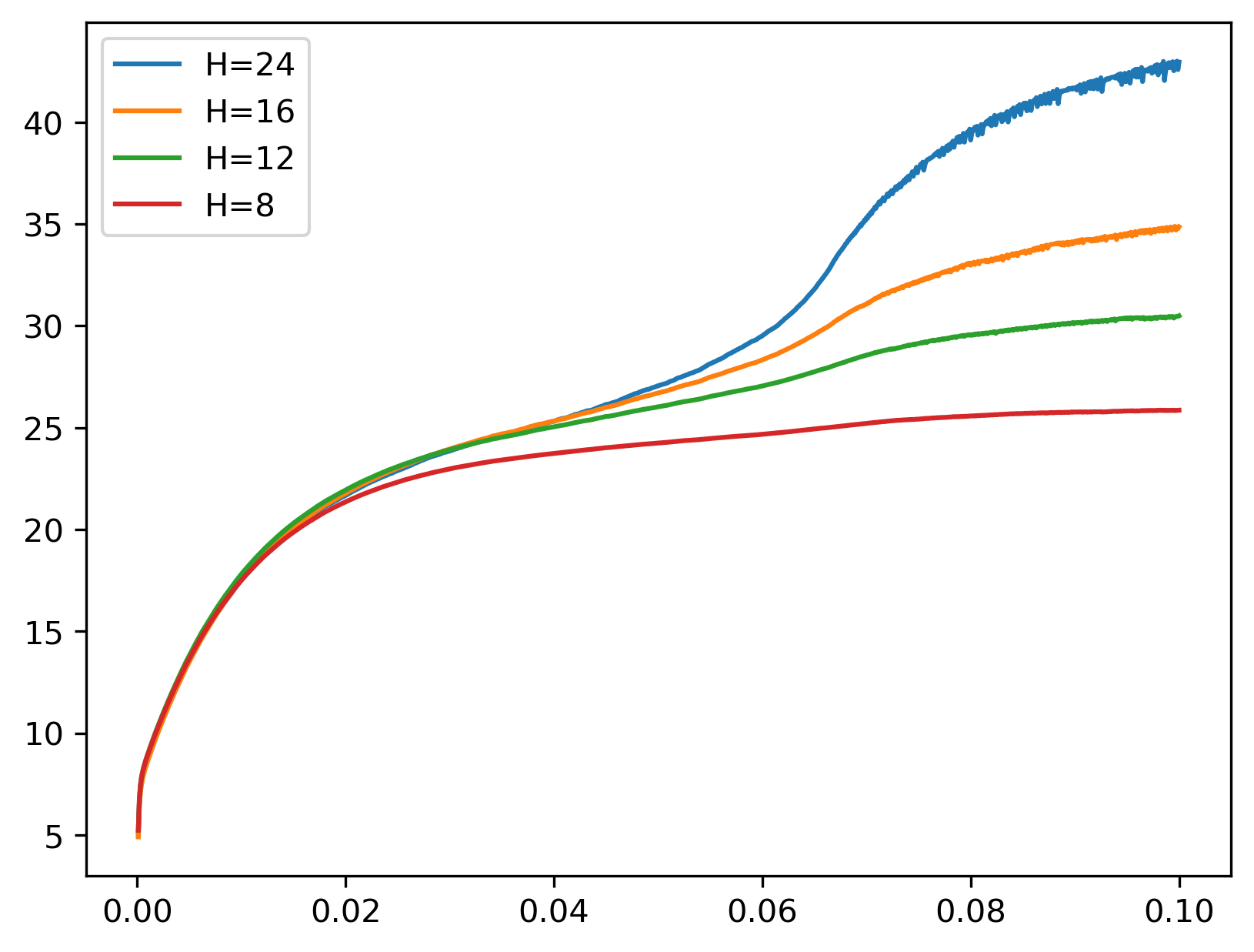
(b) $M_{0}=80$

Figure 3: Maximum of chemical concentration $c$ vs computation time $T$ with different total mass $M_{0}$.

Furthermore, if we assume, there exists a self-similar profile of $\rho$ at origin as discussed in [27] and Section 2.1, namely, $\rho(x,t)\sim\frac{1}{|x|^{2}}$, by (1), the Fourier coefficients of chemical concentration $c$ has the following asymptotics,

$$\mathcal{F}c(\omega)\sim\frac{1}{|\omega|^{2}+k^{2}}\hat{\rho}\sim\frac{1}{(|\omega|^{2}+k^{2})|\omega|}.$$ (32)

Then the maximum of $c$ in the computation shall vary vs the discretization parameter $H$. More precisely, we note at the origin,

$$c(0)\sim\int\frac{1}{(|\omega|^{2}+k^{2})|\omega|}e^{i\omega x}d\omega|_{x=0}=\int\frac{1}{(|\omega|^{2}+k^{2})|\omega|}d\omega.$$ (33)

In practical discretization, the range of integral (33) is related to the maximum frequency, namely $[-\frac{\pi}{L}(\frac{H}{2}-1),\frac{\pi}{L}\cdot\frac{H}{2}]^{3}$. Then, for the type of $\frac{1}{|x|^{2}}$ profile blow up,

$$\|c\|_{\infty}=\mathcal{O}(\ln(H)).$$ (34)

Similar analysis shows for the type of $\delta(x)$ profile blow up,

$$\|c\|_{\infty}=\mathcal{O}(H).$$ (35)

In Fig.3, we present the maximum value of $c$ vs the computational time $T$ with a different number of Fourier modes $H$ and total mass $M_{0}$. We can see in the case of a possible blow-up (Fig.3(b)), that the maximum of $c$ varies dramatically for different $H$. In the investigation following, we will use this as an indicator of a possible blow-up.

Furthermore, under the same configuration in the case of $M_{0}=80$, we take $T=1$ to achieve a numerically stable $\|c\|_{\infty}$. And test for $H$ ranging from $8$ to $24$. In Fig.4, we plot $\|c\|_{\infty}$ vs $H$ and observe that the maximum of $c$ grows near-linearly in $H$.

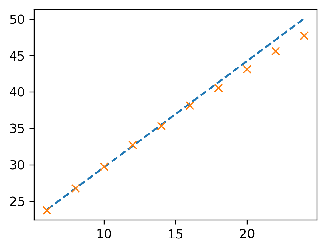
Figure 4: Maximum of $c$ vs. the number of Fourier modes $H$ (in each dimension), total mass $M_{0}=80$.

Remark 4.1.

Similar ideas that detect blow-ups by comparing maximum values computed under different discretizations, can be found in the literature on finite volume approach to 2D Keller Segel systems. For example in [4], the $\delta$ type singularities in the 2D system are identified when $\|\rho\|_{\infty}=\mathcal{O}(\frac{1}{\Delta x\Delta y})$,

4.2 Convergence over $\delta t$

Now we turn to validate the convergence of algorithms with respect to time step $\delta t$. In this regard, we consider the same initial condition ($\rho$ and $c$ at $t=0$) and physical parameters, see (31), as in the first example. Also, we keep the number of Fourier modes in each dimension as $H=24$, the number of particles $P=10000$, and computational domain $\Omega=[-L/2,L/2]^{3}$ with $L=8$. Lastly, we set $M_{0}=80$ and $T=0.01$ when the system has not formed any singularities (see Fig.3(b)). To investigate the convergence, we consider $\delta$ in the range between $2^{-8}T$ to $2^{-4}T$ and take $\delta_{ref}=2^{-11}T$ as the reference solution. In Fig.5, we compute the $L_{2}$ relative error of chemical concentration $c$ at the final time $T$. In addition, we fit the slope of error vs $\delta t$ in the logarithmic scale and find $e(\delta t)=\mathcal{O}(\delta t^{1.011})$ indicating the algorithm being approximately first order in time.

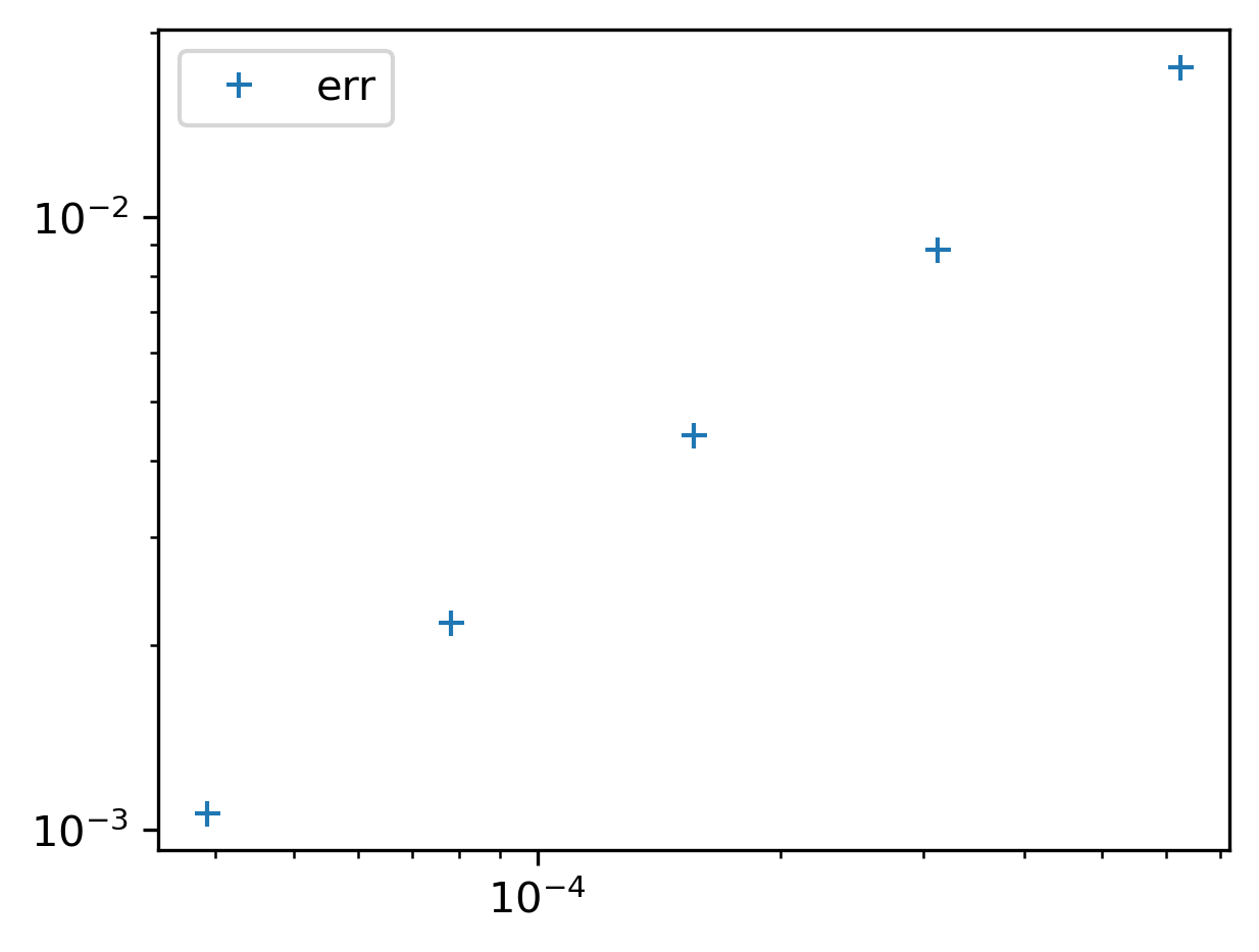
Figure 5: $L_{2}$ relative error of $c$ vs $\delta t$.

4.3 Blow up behaviors

As mentioned in Sec.2.1, it is a well-known dichotomy that $8\pi$ is the critical mass for the simplest two-dimensional parabolic-elliptic KS system (5).

1. If $M_{0}<8\pi$, the system has a global smooth solution.

2. If $M_{0}>8\pi$, the system has no global smooth solutions.

While for fully parabolic system or (5) with passive advection, no variance identity like (6) is known. One must resort to numerical computation to investigate the physical factors that lead to the possible blow-up behaviors. As suggested by the asymptotics (34) and (35), in the following examples, we will test for two cases $H=24$ and $H=12$ and comparing the $\|c\|_{\infty}$ to detect possible blowup.

Mass dependence

We start with investigating the critical mass $M_{0}$ which plays the dominant role in the dichotomy of simple 2D parabolic elliptic system (5). To this end, we initialize the algorithm with uniform distribution over the unit ball centered at the origin and $c(0,x)=0$. We then apply the algorithm with two different $H$ to compute the density and chemical concentration until $T=1$. To identify the possible blow-up, we compute the ratio of the $|c|_{\infty}$ between two cases. In Fig.6(a) we present the ratio, namely, $\frac{|c|_{\infty,H=24}}{|c|_{\infty,H=12}}$, along time with various $M_{0}$. We can see the ratio increases dramatically when a potential blow-up forms for $M_{0}\geq 47.6$. In Fig.6(b) we present the ratio at final time $T=1$, indicating that the critical mass of the aforementioned initial condition shall be between $47.6$ and $47.8$.

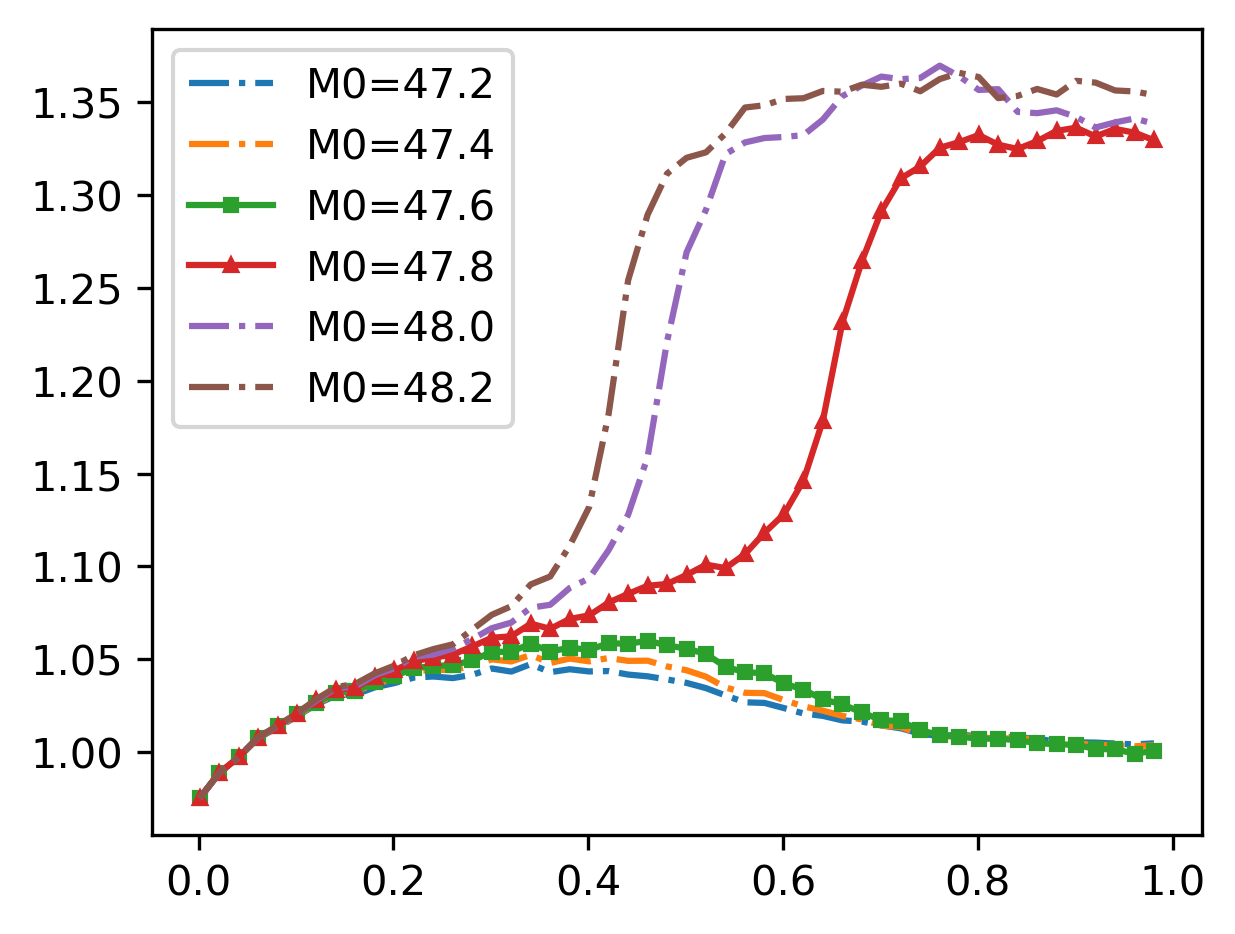
(a) $\frac{|c|_{\infty,H=24}}{|c|_{\infty,H=12}}$ vs. computation time $T$.

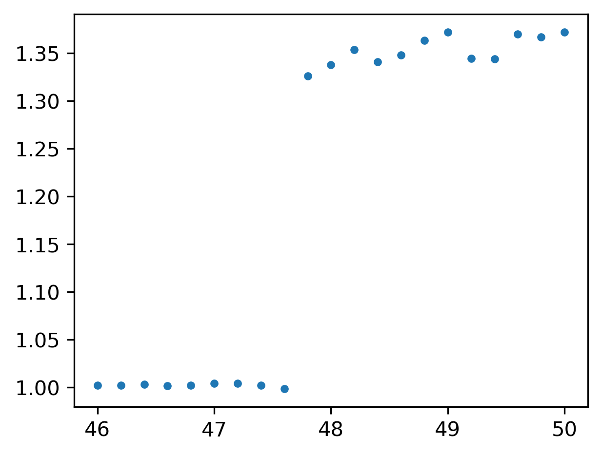
(b) $\frac{|c|_{\infty,H=24}}{|c|_{\infty,H=12}}$ at $T=1$ vs. $M_{0}$.

Figure 6: Ratio of $|c|_{\infty}$’s from 2 runs with $H=24$ and $H=12$, revealing critical mass for blowup.

Geometry dependence

Unlike the simplest parabolic-elliptic KS system (5) where the total mass is the only factor that determines the aggregation behaviors, we find experimentally that the critical mass varies for the different initial distributions of $\rho$. For example, we follow the same configuration in the experiment of finding critical mass (as shown in Fig.6) except replacing the initial distribution to be the uniform distribution on a ball centered at the origin with radius 0.8. Given a more concentrated initial distribution, we find the critical mass for the system decreases. More precisely, in Fig.7(a), we present the ratio of $|c|_{\infty}$ of various total mass $M_{0}$ vs. computational time $T$. We can see a sharp change of ratio when the total mass $M_{0}$ is large enough ($M_{0}\geq 39$) then the possible singularities have formed. While for $M_{0}$ that is relatively small ($M_{0}\leq 38.8$) the ratio is stable near $1$ over the computational time. In Fig.7,(b) we present the ratio at final time $T=0.1$ vs. total mass $M_{0}$, which indicates the critical mass for such initial condition is between $38.8$ and $39$.

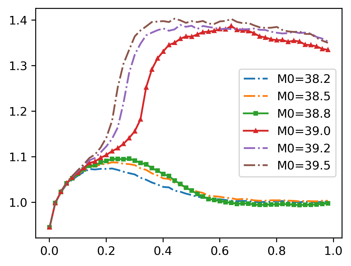
(a) $\frac{|c|_{\infty,H=24}}{|c|_{\infty,H=12}}$ vs. computation time $T$.

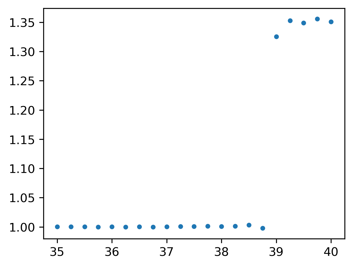
(b) $\frac{|c|_{\infty,H=24}}{|c|_{\infty,H=12}}$ at $T=1$ vs. $M_{0}$.

Figure 7: Ratio of $|c|_{\infty}$’s from 2 runs with $H=24,12$; particles stay within initial radius $0.8$.

4.4 Aggregation behaviors from non-radial initial data

In this subsection, we investigate the aggregation behaviors in more general distributions. To this end, we consider a more practical scenario where the initial distribution $\rho$ models several separated clusters of organisms and the mass in each individual cluster is below the critical mass while the total mass is super-critical. To be more concrete, we assume the initial distribution is a uniform distribution on four balls with a radius $0.5$ and centered at four vertices of a regular tetrahedron, namely,

$$\begin{pmatrix}1\\ 0\\ 0\end{pmatrix},\quad\begin{pmatrix}-\frac{1}{2}\\ \frac{\sqrt{3}}{2}\\ 0\end{pmatrix},\quad\begin{pmatrix}-\frac{1}{2}\\ -\frac{\sqrt{3}}{2}\\ 0\end{pmatrix},\quad\begin{pmatrix}0\\ 0\\ \sqrt{2}\end{pmatrix}.$$ (36)

See also Fig.8(a) for the scatter plot of particles representing the initial distribution. We assume the total mass to be $M_{0}=80$ and so each cluster has a mass of $20$ which is below the critical mass for a ball with radius $r=0.5$. Then we apply the algorithm to compute the KS system up to $T=0.5$ with $H=24$ and $H=12$ while keeping the rest of the configurations. In Fig.8(b), we compute the ratio between the maxima of $c$ vs time with two different spatial discretizations. We can see the singularities formed in the system at around $T=0.3$.

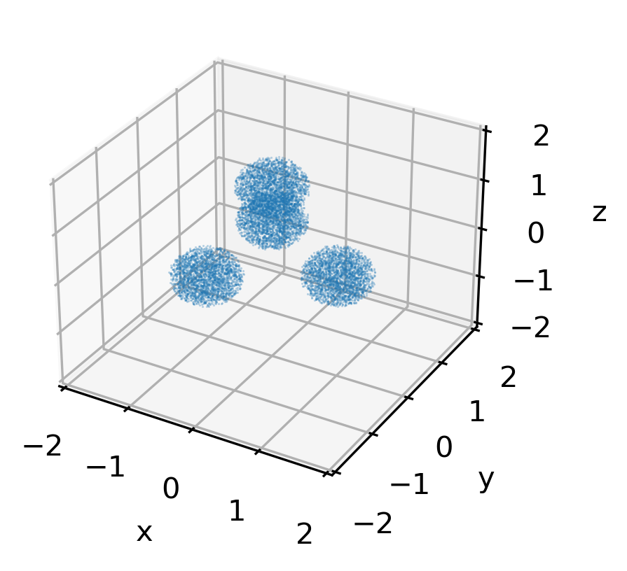
(a) Initial distribution.

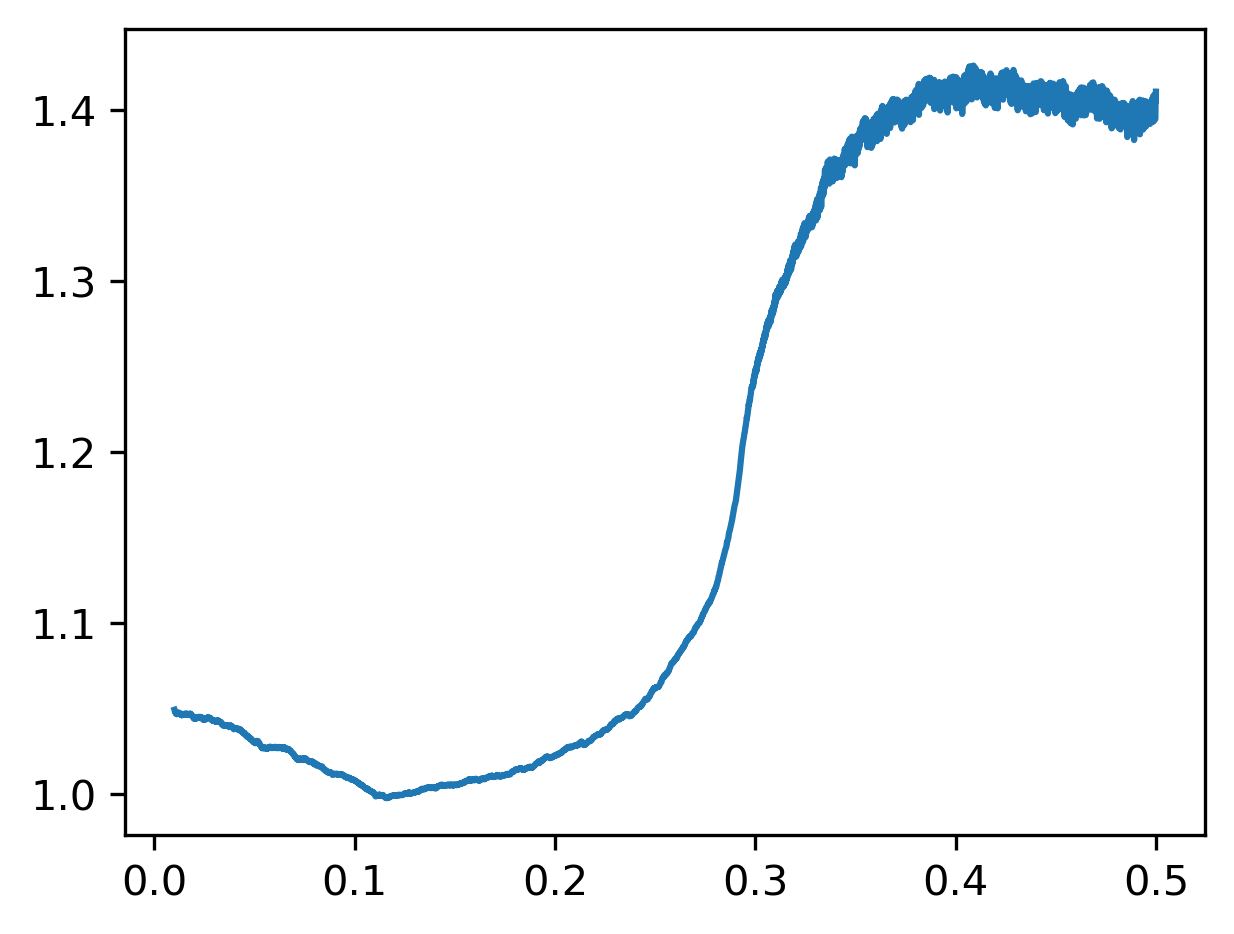
(b) $\frac{|c|_{\infty,H=24}}{|c|_{\infty,H=12}}$ vs. computation time.

Figure 8: Identifying the formation of a finite time singularity at $t\approx 0.3$ in non-radial solutions.

In Fig.9, we present the scatter plot of particles between $T=0.1$ and $T=0.4$.

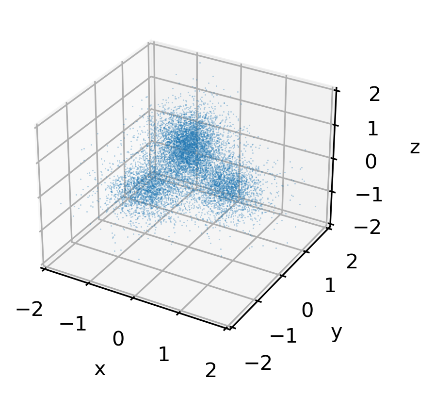
(a) $T=0.1$

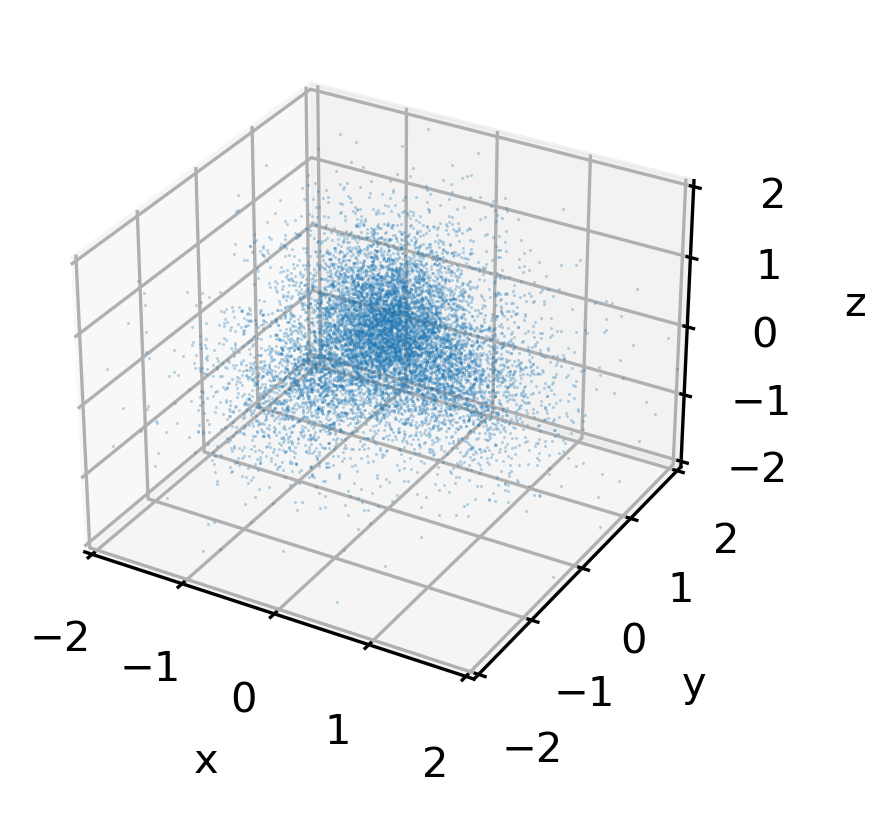
(b) $T=0.2$

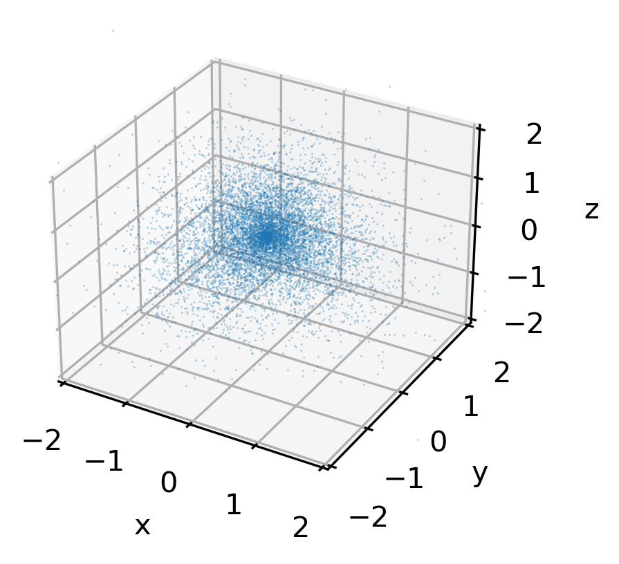
(c) $T=0.3$

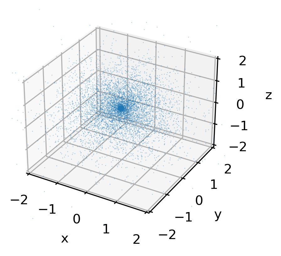
(d) $T=0.4$

Figure 9: Particle scatter plot at $T=0.1:0.1:0.4$: three cluster merging and a singularity formation.

Comparing Fig.8(a) with Fig.9(a), we can see diffusive behavior. This is due to the mass in each individual cluster being below the critical mass. Such diffusive behavior lasts until around $T=0.2$, see Fig.8(b) where the active particles form a single larger cluster. The mass of the new cluster centered at the origin is $M_{0}=80$. Then in Fig.9(c), the aggregation starts to form a singularity, which can also be seen from the sharp increase in the ratio of maximum of $c$ in Fig.8(b). Lastly, in Fig.9(d), we can directly identify the possible blow-up at the origin through the scatter plot.

4.5 Critical mass and blowup in parabolic-parabolic KS

As the last example, we access the singular solutions in the fully parabolic systems. For expository purposes, we set $\epsilon=0.1$ in (1) and keep the rest of the physical parameters. The initial condition is assumed to be a uniform distribution on a ball with radius $0.8$ and $c(x,0)=0$.

From Fig.7, we know the critical mass is around $M_{0}=39$. We apply the same computational configuration as in Fig.7, besides enlarging the domain to $L=12$ to accommodate the possible diffusive behavior. We test our algorithm in two cases, $M_{0}=40$ and $M_{0}=160$ correspondingly.

The behaviors of the system are reported in Fig.10. In Fig.10(a) and (b), we present the scatter plot of the particles representing the density $\rho$ with $M_{0}=40$ and $M_{0}=160$ correspondingly, we found that despite the initial mass $M_{0}=40$ being larger than the critical mass in the case of $\epsilon=10^{-4}$, the system does not blow-up. We report that the variance of the particles grows linearly in computational time $T$ with diffusion coefficients fitted to be $1.696$. In the absence of the chemical attractant, namely $\chi=0$, the diffusion coefficient is expected to be $4\mu=4$. While for $M_{0}=160$ the system exhibits a possible singularity at the origin. In Fig.10(c), we present the ratio of $|c|_{\infty}$ under $H=24$ and $H=12$ for both initial mass. Similar to the observation of Fig.10(a) and (b), the blow-up behavior crucially depends on a critical level of the initial mass.

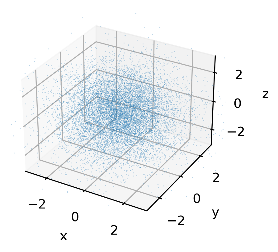
(a) Scattering plot of particles at $T=1$ with $M_{0}=40$.

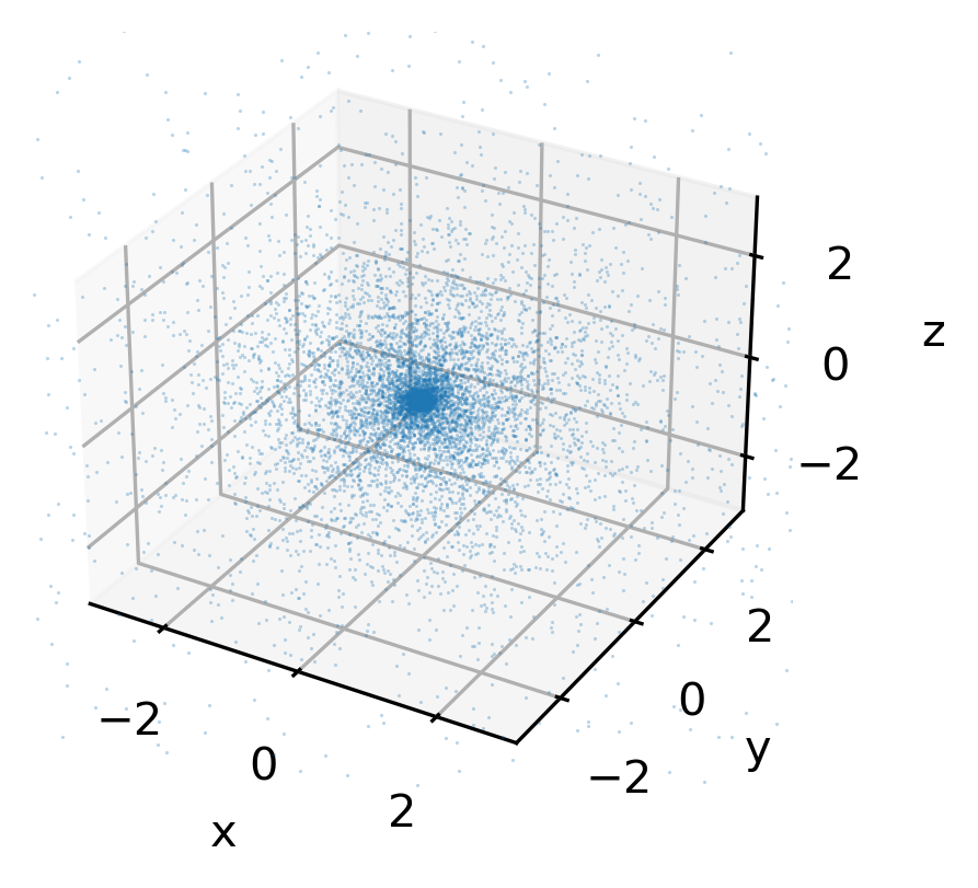
(b) Scattering plot of particles at $T=1$ with $M_{0}=160$.

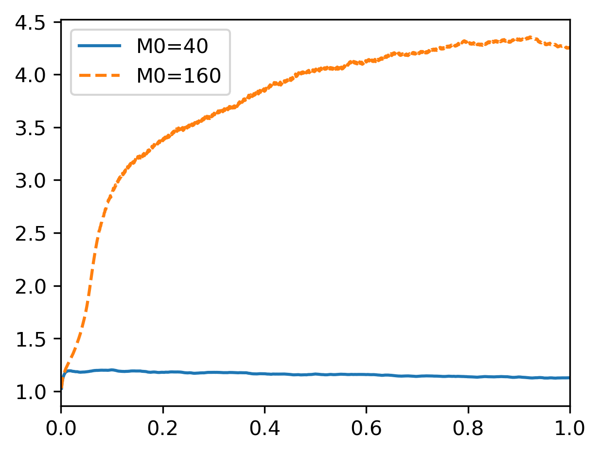
(c) $\frac{|c|_{\infty,H=24}}{|c|_{\infty,H=12}}$ vs computation time $T$ with different total mass $M_{0}$.

Figure 10: Effects of initial mass $M_{0}$ on focusing behavior (finite time blowup).

5 Concluding Remarks

We introduced a stochastic interacting particle and field algorithm, observed its convergence, and demonstrated its efficacy in computing blowup dynamics of fully parabolic KS systems in 3D from general non-radial initial data. The algorithm is recursive with no history dependence, and the field variable is computed by FFT. Due to the field variable (concentration) being smoother than the density, the FFT approach works with only dozens of Fourier modes. The aggregation or focusing behavior in the density variable is resolved by 10k particles. The algorithm successfully detected blowup through the field variable in terms of the critical amount of initial mass. The algorithm is self-adaptive and does not rely on any anzatz of blowup which is unknown except in the parabolic-elliptic KS system. A weakness is the potentially high cost of FFT in 3D when a large number of Fourier modes is required in case of a high-resolution computation near blowup time. We plan to study this issue in a future work.

References

- [1] Vincent Calvez and Lucilla Corrias. The parabolic-parabolic Keller-Segel model in . Communications in Mathematical Sciences, 6(2):417–447, 2008.
- [2] Li Chen, Shu Wang, and Rong Yang. Mean-field limit of a particle approximation for the parabolic-parabolic Keller-Segel model. arXiv preprint arXiv:2209.01722, 2022.
- [3] Wenbin Chen, Qianqian Liu, and Jie Shen. Error estimates and blow-up analysis of a finite-element approximation for the parabolic-elliptic Keller-Segel system. International Journal of Numerical Analysis and Modeling, 19(2-3):275–298, 2022.
- [4] Alina Chertock, Yekaterina Epshteyn, Hengrui Hu, and Alexander Kurganov. High-order positivity-preserving hybrid finite-volume-finite-difference methods for chemotaxis systems. Advances in Computational Mathematics, 44:327–350, 2018.
- [5] Alina Chertock and Alexander Kurganov. A second-order positivity preserving central-upwind scheme for chemotaxis and haptotaxis models. Numerische Mathematik, 111(2):169–205, 2008.
- [6] Katy Craig and Andrea Bertozzi. A blob method for the aggregation equation. Mathematics of computation, 85(300):1681–1717, 2016.
- [7] Ibrahim Fatkullin. A study of blow-ups in the Keller–Segel model of chemotaxis. Nonlinearity, 26(1):81, 2012.
- [8] Yoshikazu Giga, Noriko Mizoguchi, and Takasi Senba. Asymptotic Behavior of Type I Blowup Solutions to a Parabolic-Elliptic System of Drift–Diffusion Type. Archive for Rational Mechanics and Analysis, 201(2):549–573, 2011.
- [9] Jan Haškovec and Christian Schmeiser. Stochastic particle approximation for measure valued solutions of the 2D Keller-Segel system. Journal of Statistical Physics, 135:133–151, 2009.
- [10] Jan Haškovec and Christian Schmeiser. Convergence of a stochastic particle approximation for measure solutions of the 2D Keller-Segel system. Communications in Partial Differential Equations, 36(6):940–960, 2011.
- [11] Miguel A Herrero, E Medina, and JJL Velázquez. Self-similar blow-up for a reaction-diffusion system. Journal of Computational and Applied Mathematics, 97(1-2):99–119, 1998.
- [12] Miguel A Herrero and Juan JL Velázquez. A blow-up mechanism for a chemotaxis model. Annali della Scuola Normale Superiore di Pisa-Classe di Scienze, 24(4):633–683, 1997.
- [13] Thomas Hillen and Kevin Painter. Global existence for a parabolic chemotaxis model with prevention of overcrowding. Advances in Applied Mathematics, 26(4):280–301, 2001.
- [14] Thomas Y Hou and Ruo Li. Computing nearly singular solutions using pseudo-spectral methods. Journal of Computational Physics, 226(1):379–397, 2007.
- [15] Evelyn F Keller and Lee A Segel. Initiation of slime mold aggregation viewed as an instability. Journal of theoretical biology, 26(3):399–415, 1970.
- [16] Saad Khan, Jay Johnson, Elliot Cartee, and Yao Yao. Global regularity of chemotaxis equations with advection. Involve, a Journal of Mathematics, 9(1):119–131, 2015.
- [17] Pierre Gilles Lemarié-Rieusset. Small data in an optimal banach space for the parabolic-parabolic and parabolic-elliptic Keller–Segel equations in the whole space. Adv. Differential Equations, 18(11/12):1189–1208, 2013.
- [18] Jian-Guo Liu, Li Wang, and Zhennan Zhou. Positivity-preserving and asymptotic preserving method for 2D Keller-Segel equations. Mathematics of Computation, 87(311):1165–1189, 2018.
- [19] Jian-Guo Liu and Rong Yang. A random particle blob method for the Keller-Segel equation and convergence analysis. Mathematics of Computation, 86(304):725–745, 2017.
- [20] Jian-Guo Liu and Rong Yang. Propagation of chaos for the Keller-Segel equation with a logarithmic cut-off. Methods and Applications of Analysis, 26(4):319–348, 2019.
- [21] Guo Luo and Thomas Hou. Toward the finite-time blowup of the 3D axisymmetric Euler equations: a numerical investigation. Multiscale Modeling & Simulation, 12(4):1722–1776, 2014.
- [22] Stéphane Mischler and Clément Mouhot. Kac’s program in kinetic theory. Inventiones mathematicae, 193(1):1–147, 2013.
- [23] Noriko Mizoguchi. Global existence for the Cauchy problem of the parabolic–parabolic keller–segel system on the plane. Calculus of Variations and Partial Differential Equations, 48(3):491–505, 2013.
- [24] Clifford S Patlak. Random walk with persistence and external bias. The bulletin of mathematical biophysics, 15:311–338, 1953.
- [25] Benoît Perthame. Transport equations in biology. Springer Science & Business Media, 2006.
- [26] Jie Shen and Jie Xu. Unconditionally bound preserving and energy dissipative schemes for a class of Keller–Segel equations. SIAM Journal on Numerical Analysis, 58(3):1674–1695, 2020.
- [27] Philippe Souplet and Michael Winkler. Blow-up profiles for the parabolic–elliptic Keller–Segel system in dimensions . Communications in Mathematical Physics, 367(2):665–681, 2019.
- [28] Angela Stevens. The derivation of chemotaxis equations as limit dynamics of moderately interacting stochastic many-particle systems. SIAM Journal on Applied Mathematics, 61(1):183–212, 2000.
- [29] Angela Stevens and Hans G Othmer. Aggregation, blowup, and collapse: the abc’s of taxis in reinforced random walks. SIAM Journal on Applied Mathematics, 57(4):1044–1081, 1997.
- [30] Taiki Takeuchi. The Keller-Segel system of parabolic-parabolic type in homogeneous Besov spaces framework. Journal of Differential Equations, 298:609–640, 2021.
- [31] Zhongjian Wang, Jack Xin, and Zhiwen Zhang. A DeepParticle method for learning and generating aggregation patterns in multi-dimensional Keller-Segel chemotaxis systems. arXiv preprint arXiv:2209.00109, 2022.