I-AI: A Controllable & Interpretable AI System
for Decoding Radiologists’ Intense Focus for Accurate CXR Diagnoses

Abstract

In the field of chest X-ray (CXR) diagnosis, existing works often focus solely on determining where a radiologist looks, typically through tasks such as detection, segmentation, or classification. However, these approaches are often designed as black-box models, lacking interpretability. In this paper, we introduce Interpretable Artificial Intelligence (I-AI) a novel and unified controllable interpretable pipeline for decoding the intense focus of radiologists in CXR diagnosis. Our I-AI addresses three key questions: where a radiologist looks, how long they focus on specific areas, and what findings they diagnose. By capturing the intensity of the radiologist’s gaze, we provide a unified solution that offers insights into the cognitive process underlying radiological interpretation. Unlike current methods that rely on black-box machine learning models, which can be prone to extracting erroneous information from the entire input image during the diagnosis process, we tackle this issue by effectively masking out irrelevant information. Our proposed I-AI leverages a vision-language model, allowing for precise control over the interpretation process while ensuring the exclusion of irrelevant features.

To train our I-AI model, we utilize an eye gaze dataset to extract anatomical gaze information and generate ground truth heatmaps. Through extensive experimentation, we demonstrate the efficacy of our method. We showcase that the attention heatmaps, designed to mimic radiologists’ focus, encode sufficient and relevant information, enabling accurate classification tasks using only a portion of CXR. The code, checkpoints, and data are at https://github.com/UARK-AICV/IAI.

1 Introduction

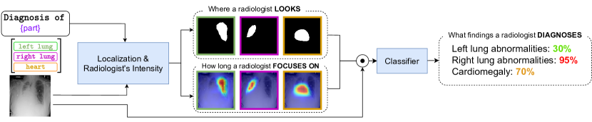
Figure 1: The overall pipeline of our proposed I-AI framework to detect radiologist’s intense focus for accurate CXR diagnoses. The model takes an CXR and anatomical prompt of a particular area of diagnosis as its inputs and outputs the answers of three key questions: where a radiologist looks, how long a radiologist focuses on specific areas, and what findings a radiologist diagnoses. $\odot$ is the Hadamard product.

Table 1: Model capacity comparison between our proposed method and related approaches.

Methods	Localization	Diagnosis	Intensity	Interpretability	Controllability
ChexNet [32]	✗	✓	✗	✗	✗
van Sonsbeek[44]	✗	✓	✗	✗	✗
Grad-CAM [39]	✓	✗	✓	✗	✗
Grad-CAM++ [4]	✓	✗	✓	✗	✗
Relevance-CAM [21]	✓	✗	✓	✗	✗
Integrated Grad-CAM [38]	✓	✗	✓	✗	✗
Rozenberg et al. [34]	✓	✓	✗	✗	✗
Karargyris et al. [17]	✓	✓	✓	✗	✗
Ours	✓	✓	✓	✓	✓

Computer-aided diagnosis (CAD) has proven to be an invaluable tool in the medical field. In chest X-ray (CXR) diagnosis, the extensive growth of deep learning has given rise to several automated models that can outperform trained radiologists [32, 27]. In contrast to fully automatic systems, a good CAD framework should also improve the radiologist’s performance [8]. Despite steady improvements in deep learning methods in medical analysis [2, 45, 42, 10, 41, 20, 30, 14, 54], there remains a problem: If the model makes a correct prediction, but the radiologist does not, then how does the system help the radiologist discern the truth? Sight is the essential first step in human thought, and radiologists must look carefully to verify whether there is an abnormality only after having extracted enough visual information [3]. Thus, to assist radiologists effectively, we must address two crucial questions: where the radiologist should look, and how focused, or intense, they should. Answering these questions allows us to explore what findings can be diagnosed based on the radiologist’s intensity.

The standard approach to address the first question is to visualize the internal features of the model using standard visualization methods, such as Class Activation Mapping (CAM) [53, 39, 46]. However, many state-of-the-art techniques are heavily reliant on the usual black-box approach. The resulting heatmaps lack reliability as there is no constraint regarding any ground truth from physicians except the final disease label. Consequently, these approaches may make use of incorrect information, such as using the diaphragm as an indirect cue for cardiomegaly [17]. Other approaches simultaneously predict the disease and point out the location of it by making predictions in the form of bounding boxes  [34, 24]. However, these approaches only address the first question of where the radiologist should look. To overcome these limitations, Karargyris et al. [17] introduces eye gaze datasets and modifies UNet [33] to generate heatmaps and predict abnormal findings. However, due to the bottleneck location prediction and classification both share, this approach encounters a significant challenge of relying on incorrect information when classifying. Clearly, to synchronously answer multiple questions would require multiple heads in the model or multiple models creating different types of heatmaps.

To address all the above problems comprehensively, we propose a novel unified controllable interpretable I-AI pipeline for simultaneously generating radiologist-based anatomic attention heatmaps and predicting abnormal findings as illustrated in Figure 1. Our I-AI model takes a CXR image and anatomical prompt as inputs. To be controllable, our model first employs a short prompt specifying an anatomical part to guide the model’s attention. To be interpretable, our model allows users to observe meaningful attention heatmaps of radiologists’ explicit focus. I-AI model not only addresses the first question of localization but also captures the radiologists’ focus intensity. Once obtaining where and how intense the radiologist gazes, our I-AI eliminates all extraneous information before predicting any abnormal findings, and therefore we ensure that our model cannot exploit erroneous data (i.e. diagnosis). This makes our network more interpretable and controllable compared to traditional black-box approaches. The I-AI model capacity comparison between our proposed method and related approaches is given in Table 1.

To obtain radiologist’s intensity, we utilize the REFLACX dataset [19], which contains a plethora of eye gaze information captured by high sensitivity hardware of radiologists analyzing CXR images. However, aligning a gaze sequence with an abnormal finding is non-trivial. For example, the radiologist’s gaze can shift from the heart to the upper left lung, then to the right lung, and go back to the heart, and then they start to say ”the heart size is normal”. The randomness in the provided gaze sequence makes it hard to manually decide exactly which gaze points contribute to the diagnosis. To handle this, we propose a semi-automatic approach to extract gaze information using anatomical parts of the lung. Using this filtered data, we train, test our method and further verify a hypothesis that the classifier can achieve strong performance even without using the full image.

Our contribution can be summarized as follows:

• We propose I-AI, a novel unified controllable & interpretable approach that uses a CXR image in conjunction with an anatomical prompt to determine the location and intensity of a radiologist’s focus followed by the prediction of a corresponding finding. To the best of our knowledge, our method is the first in the medical domain to learn from radiologist-based anatomical gaze heatmap while offering controllability.

• To train our I-AI model, we present a semi-automatic approach to extract radiologist-based anatomic heatmap from eye gaze datasets by using transcript and anatomic segmentation masks.

• We have conducted an extensive experiments and comparison to demonstrate the effectiveness of the proposed I-AI.

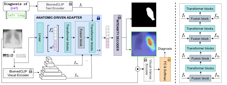
Figure 2: The detailed pipeline of our proposed controllable & interpretable framework to decode radiologist’s intense focus for accurate CXR diagnoses. In our framework, the frozen pre-trained model still serves to extract text embedding and CXR visual encoding, and the anatomic-driven adapter generates mask and attention heatmap to guide the deeper layers of the pre-trained model.

2 Related works

Explainable Deep Learning. Understanding a model’s decision-making process holds significant importance today, particularly in CAD. Recent developments such as Class Activation Mapping (CAM) [39, 38, 4, 21] have showcased one common approach: training a black box model and subsequently employing CAM-related techniques to visualize critical areas. While black-box models often exhibit high performance, they are recognized for their unreliability, as highlighted in literature [35]. Therefore, we design our model as an interpretable approach.

Interpretable Deep Learning. Unlike the aforementioned explainable tools, a more desirable approach entails the design of a system wherein decisions are intrinsically linked to explainability, particularly in high-stakes medical contexts [35]. Generally, interpretable models aim to transform inputs into human-interpretable representations such as concepts or prototypes, which are then harnessed for prediction. To imbue the model with self-explanatory capabilities, many researchers have embraced the successful prototype-based approach [5, 29, 28, 43, 36, 47, 37]. For instance, ProtoPNet [5] introduces a prototypical part network that identifies prototypical parts within input images, leveraging this insight for the final prediction. PIP-net [28] learns prototypes that align closely with human visual perception, serving as scoring sheets during classification. In a supervised conceptual framework, TCAV [18] is trained on data representing specific concepts. Adhering to the principles of interpretable models, we extend this methodology by enlisting the expertise to annotate the raw gaze sequences of a radiologist with three intentions, corresponding to three anatomical regions: left lung diagnosis, right lung diagnosis, and heart diagnosis. Subsequently, the model employs this intention-based information to diagnose the presence of anomalies.

Disease condition localization. Some works [24, 12, 34] predict a bounding box to localize diseases with the ground truth being a bounding box and disease label. There are other works [55, 31] that train the model primarily on an image-level label and extract saliency maps or use Class Activation Mapping (CAM) to obtain the location of the disease. Karargyris et al. [17] predict a heatmap, but the ground truth is a full gaze map, and their GradCAM visualization indicates that the model is unreliable as it incorporates unrelated information in classification and heatmap prediction. Unlike previous works, we utilize a unique combination of eye tracking information, the reading of the radiologist, and anatomic segmentation to generate anatomic radiologist-based heatmaps.

CXR disease classification. Disease classification using CXR images has gained much attention recently. The earliest of these efforts, ChexNet [32], is a DenseNet [15] that uses the CXR image as its direct input. Since then, many efforts that use deep learning have risen from the related areas of supervised learning [50, 40], semi-supervised learning [25, 23], and self-supervised learning [11, 1]. Besides using the full image to predict a disease, numerous studies [24, 49, 22, 44] suggest that location information of the disease can help in classification tasks. To the best of our knowledge, no existing methods use anatomic radiologist-based heatmaps in aiding and masking out irrelevant pixels in the image for classification.

3 Methodology: Proposed I-AI

3.1 Problem Formulation

Given a CXR image $x$ and an anatomical prompt $p$, i.e. ”Diagnosis of {}” as a prefix with ”left lung”, ”right lung”, or ”the heart”, our goal is to produce a radiologist-based attention heatmap $a$ and corresponding label $y$.

Generally speaking, a radiologist-based attention heatmap should match the location and intensity of radiologists’ eye gaze patterns and highlight relevant areas of the chest X-ray (CXR) for accurate diagnoses, as described in Section 4. It should also derive the predicted label from a comparable amount of visual information that a radiologist would consider.

3.2 Architecture

To capture the textual modality while maintaining a good mask prediction, we design our heatmap predictor to be a lightweight Anatomic-Driven Adapter that leverages the BiomedCLIP [52] checkpoint, which was trained on 15 million image-caption pairs in PMC-15M [52], followed by a classifier. The architecture is described in Figure 2.

Visual encoding. First, the image will be split into $16\times 16$ patches. Then, we feed the patches into the BiomedCLIP Visual Encoder. Following Xu et al. [48], we extract the intermediate features $f_{v_{i}}\in\mathbb{R}^{H/k\times W/k\times 768}$ from 4 layers, i.e., stem, $3$, $6$, and $9$.

Text encoding. Unlike visual encoding, the anatomical prompts are short and concise, so the latent features of intermediate transformer layers are not meaningful for us. Therefore, we get only the final embedding $f_{t}\in\mathbb{R}^{512}$ from the BiomedCLIP Text Encoder module.

Anatomic-Driven Adapter. Inspired by Xu et al. [48], we train a vision transformer (ViT) [9] as an Anatomic-Driven Adapter by using the domain feature from BiomedCLIP from different scales. First, the input image $x$ is split into multiple $16\times 16$ patches. Then, we use a linear projection to produce $f_{a}\in\mathbb{R}^{(14*14)\times D}$, where $D$ is the hidden dimension. We then concatenate $f_{a}$ with a scaling vector $\alpha\in\mathbb{R}^{D}$. Next, we feed the concatenated feature into multiple stacked combinations of transformer layers and fusion blocks. Specifically, we fuse the feature from layers $\{\texttt{stem},1,2,3\}$ of our adapter ViT with $\{\texttt{stem},3,6,9\}$ layers in BiomedCLIP, a 12-layer ViT-B/16, i.e. stem to stem, $3$ to $1$, $6$ to $2$, and $9$ to $3$. For each fusion step, we also feed the text embedding $f_{t}$ into the fusion block as illustrated in Figure 2 (right).

The intuition of including the scaling vector $\alpha$ is that each element in the last latent feature does not contribute equally across all anatomic parts, so the learnable scaling vector $\alpha$ allows the model to flexibly re-weight the last feature in the most suitable way to produce the final intense heatmap.

Fusion block. The fusion block has 3 inputs, the BiomedCLIP visual encoding at $i^{th}$ block $f_{v_{i}}\in\mathbb{R}^{H/k\times W/k\times 768}$, the BiomedCLIP text embedding $f_{t}\in\mathbb{R}^{768}$, and the adapter latent feature $f_{a}\in\mathbb{R}^{(14*14)\times D}$. For the visual encoding $f_{v_{i}}$, we first use a convolution layer to reduce the channel dimension, and then we perform an interpolation operation to resize the resolution to create $f_{v_{i}}^{\prime}\in\mathbb{R}^{(14*14)\times D}$. On the other side, we pass $f_{t}$ through a linear layer to project it into the fusion space with dimension of $D$ to create $f_{t}^{\prime}\in\mathbb{R}^{D}$. After that, we add them together

$$f_{a}^{\prime}=f_{a}+f_{v_{i}}^{\prime}+f_{t}^{\prime}$$ (1)

where the add operation of $f_{t}^{\prime}$ is broadcasting. A fusion block is shown in Figure 3(b).

We use the add operation for feature fusion: a simple and strong established baseline [48]. While other fusion mechanisms may enhance performance, they are beyond the scope of this paper.

Intensity Decoder. The Intensity Decoder receives the output of the last layer of our adapter to generate the heatmap, i.e. latent feature $f_{a}^{o}\in\mathbb{R}^{(14*14)\times D}$ and scaling vector $\alpha^{o}\in\mathbb{R}^{D}$. We first pass those two features into two separated multilayer perceptrons (MLPs). We then use matrix multiplication between them to produce a small gray-scale attention logit $a_{l}\in\mathbb{R}^{(14*14)}$. To get the final attention logit, we resize $a_{l}$ into $\hat{a_{l}}\in\mathbb{R}^{W\times H}$. In our implementation, we set $D$ to $240$. Fig. 3(a) illustrates Intensity Decoder module.

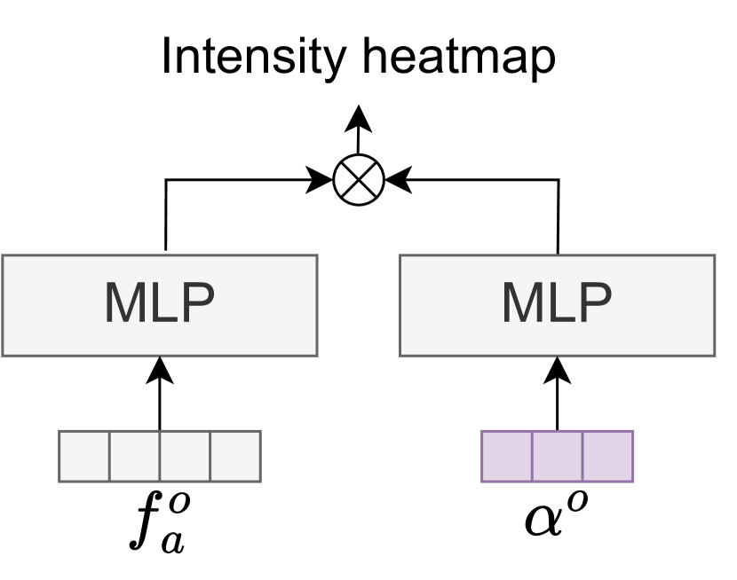
(a)

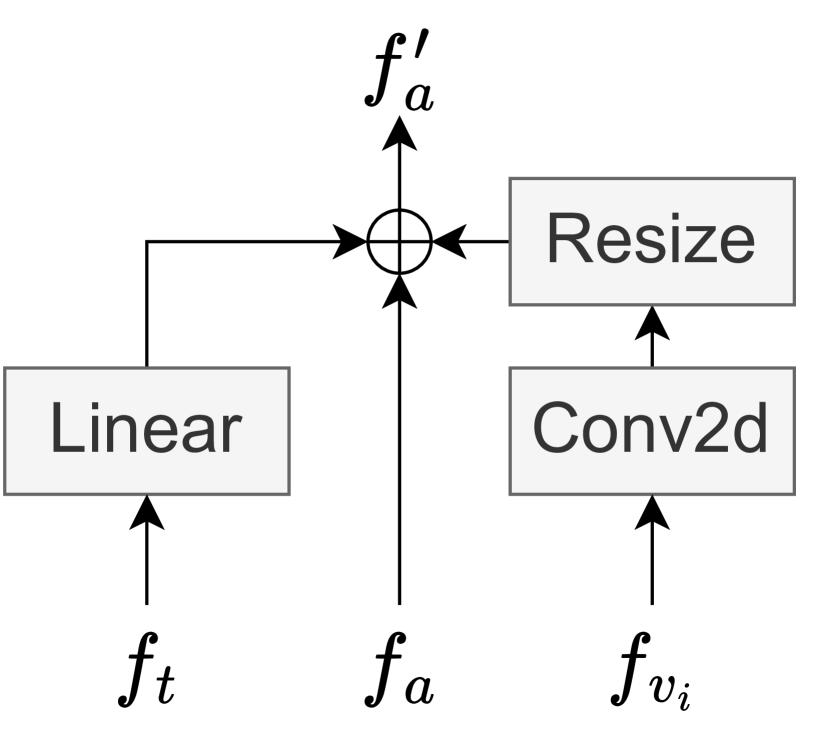
(b)

Figure 3: The detailed illustration of our proposed modules: (a) Intensity Decoder module takes the output [$f^{o}_{a}$ $\alpha^{o}$] from Anatomic-Driven Adapter as its input and results in intensity heapmap; (b) Fusion block consists of three inputs of text embedding $f_{t}$, visual encoding $f_{v_{i}}$ and adapter latent feature $f_{a}$. $\bigoplus$ denotes element-wise addition.

 

Heatmap loss. Given the predicted logit $\hat{a_{l}}\in\mathbb{R}^{W\times H}$ and ground truth heatmap $a\in\mathbb{R}^{W\times H}$, we compute the $L_{2}$ loss:

$$L_{2}=\|a_{l}-\sigma^{-1}(a)\|_{2}$$ (2)

where $\sigma^{-1}(x)=\ln{\frac{x}{1-x}}$ is the logit function. Note that we compute the loss before applying the sigmoid function to the predicted logit heatmap to avoid the issue of vanishing gradients.

Mask-related losses. Given the predicted logit $\hat{a_{l}}$ and ground truth heatmap $a$, we use binary cross entropy loss and dice loss on the masks created from $a_{l}$ and $a$. First, we apply the sigmoid function $\sigma(x)=1/(1+\exp(-x))$ on the predicted logit to create the predicted heatmap $\hat{a}$. We then define a function $f(\cdot)$:

$$f(a_{i,j})=\begin{cases}1&\text{ if }a_{i,j}>0\\ 0&\text{ otherwise}\end{cases}$$ (3)

We apply $f(\cdot)$ on all values of $a$ and $\hat{a}$ to create the ground truth mask $m$ and predicted mask $\hat{m}$. Finally, we apply the standard dice loss $L_{dice}$ and binary cross entropy loss $L_{ce}$ as in [7]. The the final loss for training the Anatomic-Driven Adapter is

$$L_{h}=\lambda_{1}L_{2}+\lambda_{2}L_{ce}+\lambda_{3}L_{dice}$$ (4)

where the weights $\lambda_{1},\lambda_{2},\lambda_{3}$ are all set to $1.0$.

Classifier. Using the predicted heatmap $\hat{a}\in[0,1]^{W\times H}$ from the previous step, we multiply $\hat{a}$ with the image $x$ element-wise to re-weight the importance of all pixels. Afterwards, we use a Visual Intense Encoder and Linear layer followed by Softmax activation as Classifier to extract and predict the finding label $y$. In our implementation, the Visual Intense Encoder is the BiomedCLIP Visual Encoder. Finally, we use a cross entropy loss to guide the classifier.

4 Data preparation

4.1 Settings

REFLACX [19] provides eye gaze data for more than 2,500 CXRs from MIMIC-CXR [16], where each gaze sequence is captured using a device with sensitivity of $1000$Hz. However, REFLACX does not provide a gaze map for each anatomic part of the lung. To construct the disease-level gaze heatmap ground truth, we manually annotate the data. The process of creating the ground truth is discussed in Sections 4.2 and 4.3. Note that the only category that has more than $300$ samples after annotating is Cardiomegaly. Therefore, Cardiomegaly is treated as a separate subset, while all other diseases are categorized into left or right lung subsets. After labeling the data, we split it into four distinct settings below

• C: Only samples with verbal transcript that specifically mentions cardiomegaly.

• L: Only samples with transcript that specifically mentions left lung.

• R: Only samples with transcript that specifically mentions right lung.

• M: Merging all samples from C, L, and R.

For each subset, we split 70% for training, 15% for evaluation, and 15% for testing. We also keep the balance between positive and negative ratio to be 1:1. The data distribution is shown in Table 2.

Table 2: Data distribution corresponding to four distinct settings: C: cardiomegaly, L: Left lung, R: Right lung, M: entire chest and merging all samples from the C, L, and R subsets.

Settings	No. samples (train:val:test)
C	611:131:132
L	631:143:145
R	575:129:125
M	1817:403:402

4.2 Ground truth heatmap

To create the ground truth heatmap, we perform two steps: make anatomic masks and filter fixations. Figure 4 demonstrates the overall pipeline for making ground truth gaze heatmaps.

Anatomic masks. REFLACX also does not provide anatomic masks, so we have to create these masks as well. Currently, the anatomic masks for three big parts are provided by EGD-CXR [17]: left lung, right lung, and the mediastinum. We finetune SAMed [51] on EGD-CXR, then use the finetuned model to make inferences on REFLACX. Then, we manually correct the segmentation masks if there is any problem. For example, we heuristically cut out the top one third of each mediastinum mask to make the heart masks, but automatic script may cut too much, so we have to fix it.

Filtering fixation sequence. For a particular anatomic region, we can acquire the fixations by looking for keywords in the provided transcripts. For example, cardiomegaly or enlarged and cardiac for setting C. Then, we will pick the rightmost sentence to decide the upper end of the interval containing our desired fixations. Specially, given a sequence of sentences $\{s_{1},s_{2},\dots,s_{n}\}$, if we find $s_{3},s_{4}$ and $s_{10}$ contain the keyword, we will use $s_{10}$. As a result, the chosen fixations are in interval $[0,e]$, where $e$ is the ending time of $s_{10}$. Using the predicted mask from before, we exclude any fixation point located beyond its boundaries. Note that the starting time of $0$ is required to capture potentially relevant visual information from the moment the radiologist takes their very first glance. Finally, by applying a Gaussian filter with radius of $150$ on the chosen fixations’ coordinates, we obtain the final ground truth heatmap. More details can be found in our Supplementary Material.

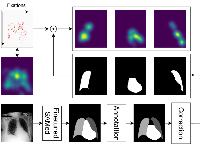
Figure 4: The pipeline of creating ground truth gaze map from eye gaze dataset.

Anatomical prompt. We also need the input prompt to guide the model. For our anatomical prompt, we use the prefix ”diagnosis of {}”. After the prefix, we append our target: ”left lung” for left lung heatmap prediction, ”right lung” for right lung heatmap, and ”heart” for heart heatmap.

In order to ensure the validity of the results and the effectiveness of the automated process, all corrections are meticulously examined and carried out by expert radiologists.

4.3 Classification

Based on our four distinct settings, we design four yes/no questions for classifying findings:

• C: Is there cardiomegaly?

• L: Is there a finding (excluding Cardiomegaly) in the left lung of the image?

• R: Is there a finding (excluding Cardiomegaly) in the right lung of the image?

• M: Is there a finding in the masked image?

Relevance-CAM [21]
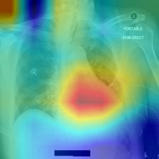
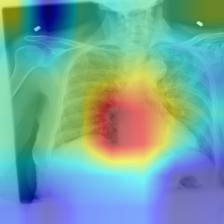
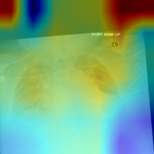
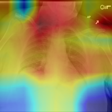
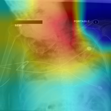
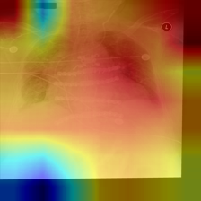
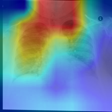
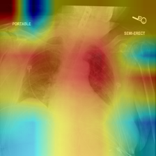
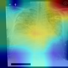
Grad-CAM [39]
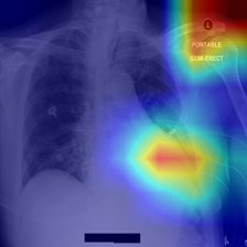
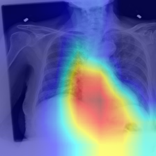
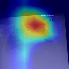
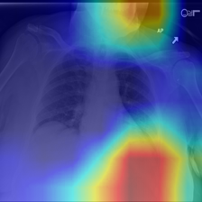
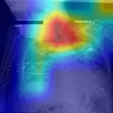
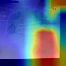
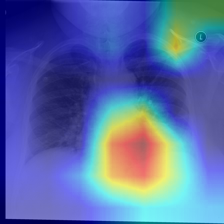
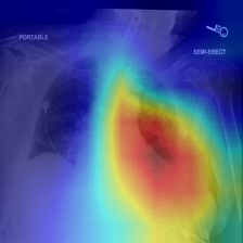
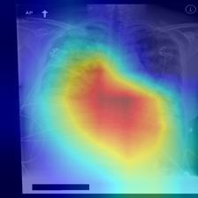
Grad-CAM++ [4]
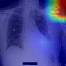
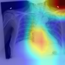
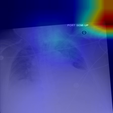
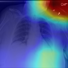
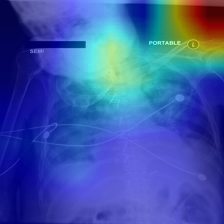
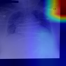
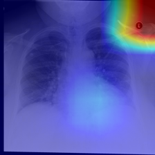
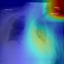
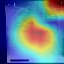
Integrated Grad-CAM [38]
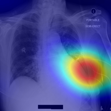
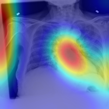
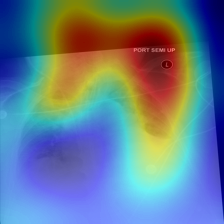
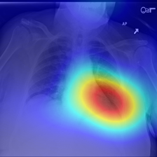
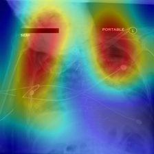
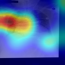
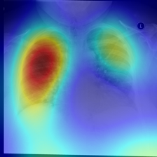
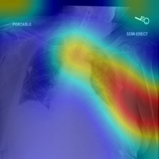
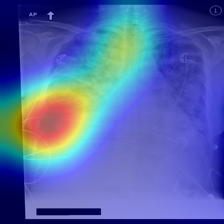
Grad-CAM  Karargyris et al. [17]
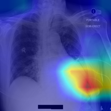
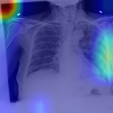
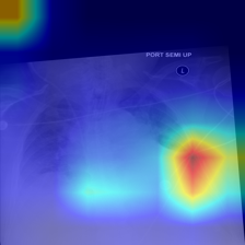
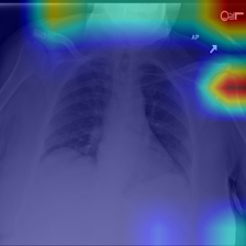
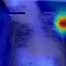
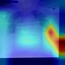
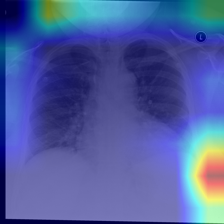
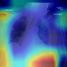
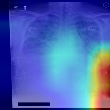
Karargyris et al. [17]
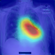
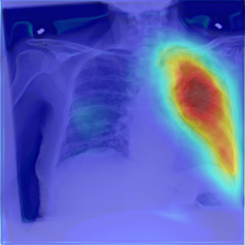
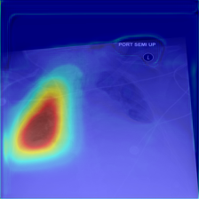
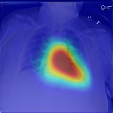
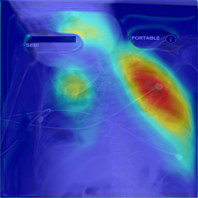
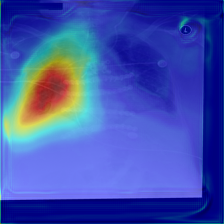
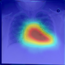
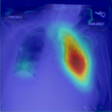
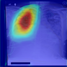
Ground truth
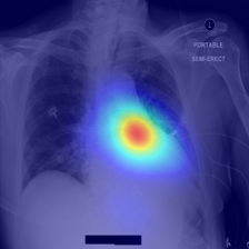
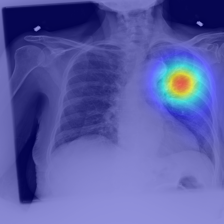
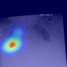
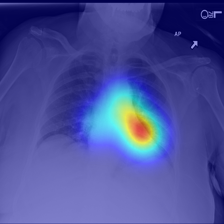
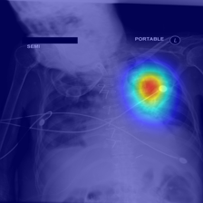
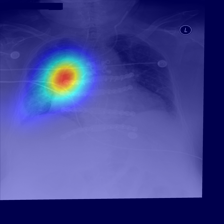
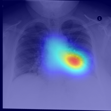
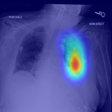
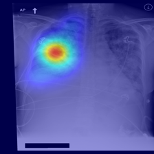
I-AI (Ours)

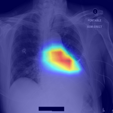
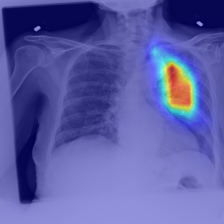
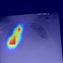
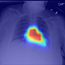
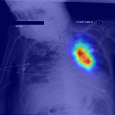
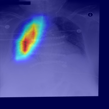
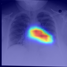
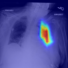
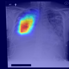
Figure 5: Comparison of the results from various CAM methods, Karargyris et al. [17], and ours. Relevance-CAM [21], Grad-CAM [39], and Grad-CAM++ [4] disappoint with unreliable heatmaps. Integrated Grad-CAM [38] exhibits some promise despite imprecision and error. Karargyris et al. [17] performs well. However, our approach stands out as the closest match to the ground truth.

5 Experiments and Results

5.1 Experiment settings

Implementation details. The ViT adapter is an $8$-layer vision transformer with dimension of $240$, $6$ attention heads, and an input patch size of $16\times 16$. The BiomedCLIP’s visual encoder is a $12$-layer ViT-B/16 pretrained on resolution $224^{2}$. The BiomedCLIP’s text encoder is a $12$-layer BERT with a vocab size of $30,522$. We freeze both the text encoder and visual encoder of BiomedCLIP in the heatmap prediction and classification stages. The MLPs in the Intensity Decoder have $3$ fully connected layers and hidden dimension of $256$. We proceed to train them with a learning rate of $0.0001$, batch size of $16$, $60,000$ iterations, and AdamW optimizer [26]. The training process takes roughly 4 hours on a single Quadro RTX 8000 GPU. The hyper-parameter and fusion layer choices are described in Supplementary Materials.

Comparison. For the black-box approaches, we train a ResNet-101 [13] on our settings. Then we use Relevance-CAM [21], Grad-CAM [39], Grad-CAM++ [4], and Integrated Grad-CAM [38] to get the performance of various CAM methods. For the heatmap prediction approach, we use Karargyris et al. [17] and TransUNet [6] to compare with our proposed method. Note that, both ResNet-101 and Karargyris et al. are trained on separated settings, i.e. C, L, and R subsets, because we have one input with three outputs. Then, we take the average of all subsets to get the final scores. Meanwhile, our proposed method is trained on only M subset.

Metrics. To quantify the performance at capturing radiologist’s intensity, we use the mean of $L_{2}$ (mL2), $L_{1}$ (mL1), Structural SIMilarity (mSSIM), and peak signal-to-noise ratio (mPSNR) over all samples. On the other hand, we also need to measure how well the heatmap can filter out irrelevant pixels by using intersection over union on foreground (fgIoU) and background (bgIoU). Additionally, we also use Frequency Weighted IoU (fwIoU).

5.2 Qualitative results

Figure 5 shows the difference of our results compared to other results from Karargyris et al. [17] and CAM methods. Despite being trained on 3 different subsets, the CAM methods produce bad and unreliable heatmaps because we do not constrain them. Note that, although Karargyris et al.’s predicted heatmap is not too far off and its accuracy is 75% (Table 4), its Grad-CAM visualizations show that Karargyris et al. is using mostly irrelevant information to classify and produce heatmaps. Unlike the aforementioned results, our method produces more precise heatmaps thanks to the radiologist-based heatmap constraint.

Moreover, we can also see from Figure 5 that Karargyris et al. [17] results are bigger than ours. Therefore, it has a better chance at covering the ground truth heatmap and has a better chance at achieving a high fgIoU score with a high false positive rate. However, the score for the intensity should not be as high because there are many regions that should be paid much less attention.

5.3 Quantitative Results

Table 3 shows that our method achieves superior performance over other heatmap generators. Among the CAM-based methods, Integrated Grad-CAM is the highest scoring, but its scores are still lower than methods that directly predict heatmaps. For instance, Integrated Grad-CAM has a fgIoU score lower than ours by approximately $25$ units. In terms of ”where to look at”, Karargyris et al.’s IoU scores closely match our method. In particular, ours has a slightly lower fgIoU than Karargyris et al. by $1.3$, but our method has a better bgIoU by approximately $9$ unit.

In regards to intensity-type metrics, our method is superior in all metrics. Specifically, our methods outperform Karargyris et al. with $+0.28$ mSSIM, $+4.49$ mPSNR, $-0.08$ m$L_{1}$, and $-0.03$ $mL_{2}$. This agrees with our visual analysis in Figure 5.

Table 3: Performance comparison with state-of-the-art methods. Our I-AI stands out for its fine-grained localization and precision. Note that Grad-CAM (Karargyris et al. [17]) method extracts the heatmap from Karargyris et al. [17] using Grad-CAM.

Methods	Location			Intensity
	fgIoU$\uparrow$	bgIoU$\uparrow$	fwIoU$\uparrow$	mSSIM$\uparrow$	mPSNR$\uparrow$	mL1$\downarrow$	mL2$\downarrow$
Relevance-CAM [21]	15.49	40.00	37.25	0.10	5.64	0.50	0.29
Grad-CAM [39]	18.91	78.12	71.49	0.24	10.40	0.22	0.11
Grad-CAM++ [4]	8.76	79.85	71.88	0.20	10.69	0.20	0.09
Integrated Grad-CAM  [38]	12.27	82.44	74.58	0.37	12.48	0.17	0.07
Grad-CAM (Karargyris et al. [17])	6.68	54.81	49.97	0.36	9.62	0.27	0.12
Karargyris et al. [17]	39.59	83.69	79.26	0.55	13.77	0.16	0.05
TransUNet [6]	33.68	90.13	84.54	0.83	12.79	0.09	0.06
I-AI (Ours)	37.27	92.44	86.96	0.83	18.26	0.08	0.02

Table 4 shows that our pipeline achieves the highest accuracy at 76%, despite using only a portion of the input image based on our predicted attention heatmap. Note that our accuracy is similar to Karargyris et al.’s, implying that using a radiologist-based heatmap to mask the input image does not harm, and might even enhance overall performance.

Table 4: Accuracy comparison between all classifiers.

Model	Accuracy(%)
Resnet-101	71.64
Karargyris et al.	75.12
TransUNet	74.88
I-AI (Ours)	76.86

5.4 Ablation study

Heatmap prediction of particular setting. Table 5 shows the robustness of our model across all settings. Our model achieves high performance with marginal difference between the full setting (M) versus subsetting C, L, and R.

Table 5: Ablation study: Heatmap prediction of particular settings.

Settings	fwIoU$\uparrow$	mSSIM$\uparrow$	mPSNR$\uparrow$	mL1$\downarrow$
C	87.42	0.84	18.80	0.07
L	86.51	0.85	18.76	0.08
R	87.16	0.82	17.48	0.10
M	86.96	0.83	18.26	0.08

The importance of mask-related losses. During training process, we notice that the gradient flow of $L_{2}$ is not enough for the model to learn where to look, and it can easily collapse to a local minima where a metric like mL2 is good, but other metrics like fgIoU are bad. As shown in Table 6, fgIoU dramatically drops to $4.06$, while mL2 is $0.03$. Therefore, we use masks created from the heatmaps together with cross entropy loss and dice loss to guide the model.

Table 6: Ablation study: the impact of losses on heatmap predictor.

Losses			Location		Intensity
$L_{2}$	$L_{ce}$	$L_{dice}$	fgIoU$\uparrow$	fwIoU$\uparrow$	mPSNR$\uparrow$	mL2$\downarrow$
✓	✗	✗	4.06	81.80	16.62	0.03
✗	✓	✓	38.16	85.04	13.11	0.04
✓	✓	✓	37.27	86.96	18.26	0.02

The importance of scaling vector $\alpha$. We define a learnable scaling vector $\alpha$ in Section 3.2 to help the model learn. From the output $f_{a}^{o}\in\mathbb{R}^{W\times H\times D}$, it is true that we can naively create the final output by taking the mean of the last dimension. However, as shown in Table 7, the inflexibility of naively averaging the feature space effectively prevents the model from learning.

Table 7: Ablation study: the scaling vector on anatomic-driven heatmap predictor.

Settings	fwIoU$\uparrow$	mSSIM$\uparrow$	mPSNR$\uparrow$	mL1$\downarrow$
w/o $\alpha$	62.87	0.31	12.59	0.17
w/ $\alpha$	86.96	0.83	18.26	0.08

The importance of radiologist-based heatmap in classification. As shown in Table 8, the classifier can be improved by using the ground truth heatmap. The area ratio is defined as $\frac{H}{T}$, where $H$ is the number of heatmap values larger than $0$, and $T$ is the number of pixels. Even though the predicted heatmaps cover more area, the performance does not scale accordingly. We can see that correctly identifying where and how long to look is more beneficial than simply covering a larger part of the image.

Table 8: Ablation study: classification performance using predicted gaze map versus ground truth gaze map.

Settings	Heatmap	Area ratio (%)	Accuracy(%)
C	Ground truth	21.49	83.33
	Ours	43.31	80.30
L	Ground truth	16.43	81.37
	Ours	43.14	74.48
R	Ground truth	18.18	80.00
	Ours	43.95	75.20
M	Ground truth	18.18	81.34
	Ours	43.49	76.86

6 Conclusion

We present I-AI, a novel unified controllable & interpretable pipeline to decode and reconstruct radiologists’ intense focus and diagnosis from CXR. Our I-AI model can simultaneously address three critical questions: where a radiologist looks, how long a radiologist focuses on specific areas, and what findings a radiologist diagnoses. Our I-AI achieves effective interpretability by aligning the output (findings) with intermediate layers (heatmap) and controllability through prompt-guided intensity generation and finding classification. Extensive experiment shows the superiority of our I-AI approach compared to other methods, even when utilizing only a portion of the image. This highlights the importance of focusing on the most relevant regions rather than processing the entire input indiscriminately.

References

- [1] Shekoofeh Azizi, Basil Mustafa, et al. Big self-supervised models advance medical image classification. In CVPR, pages 3478–3488, 2021.
- [2] Nhat-Tan Bui, Dinh-Hieu Hoang, Minh-Triet Tran, and Ngan Le. Sam3d: Segment anything model in volumetric medical images. arXiv preprint arXiv:2309.03493, 2023.
- [3] Lindsay P Busby, Jesse L Courtier, and Christine M Glastonbury. Bias in radiology: the how and why of misses and misinterpretations. Radiographics, 38(1):236–247, 2018.
- [4] Aditya Chattopadhay, Anirban Sarkar, et al. Grad-cam++: Generalized gradient-based visual explanations for deep convolutional networks. In WACV, pages 839–847. IEEE, 2018.
- [5] Chaofan Chen, Oscar Li, Daniel Tao, Alina Barnett, Cynthia Rudin, and Jonathan K Su. This looks like that: deep learning for interpretable image recognition. Advances in neural information processing systems, 32, 2019.
- [6] Jieneng Chen, Yongyi Lu, et al. Transunet: Transformers make strong encoders for medical image segmentation. arXiv preprint arXiv:2102.04306, 2021.
- [7] Bowen Cheng, Ishan Misra, Alexander G Schwing, Alexander Kirillov, and Rohit Girdhar. Masked-attention mask transformer for universal image segmentation. In CVPR, pages 1290–1299, 2022.
- [8] Kunio Doi. Computer-aided diagnosis in medical imaging: historical review, current status and future potential. Computerized medical imaging and graphics, 31(4-5):198–211, 2007.
- [9] Alexey Dosovitskiy, Lucas Beyer, et al. An image is worth 16x16 words: Transformers for image recognition at scale. arXiv preprint arXiv:2010.11929, 2020.
- [10] Jan Egger, Christina Gsaxner, Antonio Pepe, Kelsey L Pomykala, Frederic Jonske, Manuel Kurz, Jianning Li, and Jens Kleesiek. Medical deep learning—a systematic meta-review. Computer methods and programs in biomedicine, 221:106874, 2022.
- [11] Matej Gazda, Ján Plavka, Jakub Gazda, and Peter Drotar. Self-supervised deep convolutional neural network for chest x-ray classification. IEEE Access, 9:151972–151982, 2021.
- [12] Yan Han, Chongyan Chen, et al. Knowledge-augmented contrastive learning for abnormality classification and localization in chest x-rays with radiomics using a feedback loop. In WACV, pages 2465–2474, 2022.
- [13] Kaiming He, Xiangyu Zhang, Shaoqing Ren, and Jian Sun. Deep residual learning for image recognition. In CVPR, pages 770–778, 2016.
- [14] Ngoc-Vuong Ho, Tan Nguyen, Gia-Han Diep, Ngan Le, and Binh-Son Hua. Point-unet: A context-aware point-based neural network for volumetric segmentation. In MICCAI, pages 644–655. Springer, 2021.
- [15] Gao Huang, Zhuang Liu, et al. Densely connected convolutional networks. In CVPR, pages 4700–4708, 2017.
- [16] Alistair EW Johnson, Tom J Pollard, et al. Mimic-cxr, a de-identified publicly available database of chest radiographs with free-text reports. Scientific data, 6(1):317, 2019.
- [17] Alexandros Karargyris, Satyananda Kashyap, Ismini Lourentzou, et al. Creation and validation of a chest x-ray dataset with eye-tracking and report dictation for ai development. Scientific data, 2021.
- [18] Been Kim, Martin Wattenberg, et al. Interpretability beyond feature attribution: Quantitative testing with concept activation vectors (tcav). In ICML, pages 2668–2677. PMLR, 2018.
- [19] Ricardo Bigolin Lanfredi, Mingyuan Zhang, et al. Reflacx: Reports and eye-tracking data for localization of abnormalities in chest x-rays, 2021.
- [20] Ngan Le, Toan Bui, Viet-Khoa Vo-Ho, Kashu Yamazaki, and Khoa Luu. Narrow band active contour attention model for medical segmentation. Diagnostics, 11(8):1393, 2021.
- [21] Jeong Ryong Lee, Sewon Kim, et al. Relevance-cam: Your model already knows where to look. In CVPR, pages 14944–14953, 2021.
- [22] Zhe Li, Chong Wang, et al. Thoracic disease identification and localization with limited supervision. In CVPR, pages 8290–8299, 2018.
- [23] Fengbei Liu, Yu Tian, et al. Self-supervised mean teacher for semi-supervised chest x-ray classification. In Machine Learning in Medical Imaging: 12th International Workshop, MLMI 2021, pages 426–436. Springer, 2021.
- [24] Jingyu Liu, Gangming Zhao, et al. Align, attend and locate: Chest x-ray diagnosis via contrast induced attention network with limited supervision. In CVPR, pages 10632–10641, 2019.
- [25] Quande Liu, Lequan Yu, et al. Semi-supervised medical image classification with relation-driven self-ensembling model. IEEE transactions on medical imaging, 39(11):3429–3440, 2020.
- [26] Ilya Loshchilov and Frank Hutter. Decoupled weight decay regularization. arXiv preprint arXiv:1711.05101, 2017.
- [27] Mohammad Amin Morid, Alireza Borjali, and Guilherme Del Fiol. A scoping review of transfer learning research on medical image analysis using imagenet. Computers in biology and medicine, 128:104115, 2021.
- [28] Meike Nauta, Jörg Schlötterer, Maurice van Keulen, and Christin Seifert. Pip-net: Patch-based intuitive prototypes for interpretable image classification. In CVPR, pages 2744–2753, 2023.
- [29] Meike Nauta, Ron Van Bree, and Christin Seifert. Neural prototype trees for interpretable fine-grained image recognition. In CVPR, pages 14933–14943, 2021.
- [30] Tan Nguyen, Binh-Son Hua, and Ngan Le. 3d-ucaps: 3d capsules unet for volumetric image segmentation. In MICCAI, pages 548–558. Springer, 2021.
- [31] Xi Ouyang, Srikrishna Karanam, et al. Learning hierarchical attention for weakly-supervised chest x-ray abnormality localization and diagnosis. IEEE transactions on medical imaging, 40(10):2698–2710, 2020.
- [32] Pranav Rajpurkar, Jeremy Irvin, et al. Chexnet: Radiologist-level pneumonia detection on chest x-rays with deep learning. arXiv preprint arXiv:1711.05225, 2017.
- [33] Olaf Ronneberger, Philipp Fischer, and Thomas Brox. U-net: Convolutional networks for biomedical image segmentation. In MICCAI, pages 234–241. Springer, 2015.
- [34] Eyal Rozenberg, Daniel Freedman, and Alex Bronstein. Localization with limited annotation for chest x-rays. In Machine Learning for Health Workshop, pages 52–65. PMLR, 2020.
- [35] Cynthia Rudin. Stop explaining black box machine learning models for high stakes decisions and use interpretable models instead. Nature machine intelligence, 1(5):206–215, 2019.
- [36] Dawid Rymarczyk, Łukasz Struski, Michał Górszczak, Koryna Lewandowska, Jacek Tabor, and Bartosz Zieliński. Interpretable image classification with differentiable prototypes assignment. In ECCV, pages 351–368. Springer, 2022.
- [37] Dawid Rymarczyk, Łukasz Struski, Jacek Tabor, and Bartosz Zieliński. Protopshare: Prototypical parts sharing for similarity discovery in interpretable image classification. In Proceedings of the 27th ACM SIGKDD, pages 1420–1430, 2021.
- [38] Sam Sattarzadeh, Mahesh Sudhakar, et al. Integrated grad-cam: Sensitivity-aware visual explanation of deep convolutional networks via integrated gradient-based scoring. In ICASSP, pages 1775–1779. IEEE, 2021.
- [39] Ramprasaath R Selvaraju, Michael Cogswell, et al. Grad-cam: Visual explanations from deep networks via gradient-based localization. In CVPR, pages 618–626, 2017.
- [40] Sina Taslimi, Soroush Taslimi, et al. Swinchex: Multi-label classification on chest x-ray images with transformers. arXiv preprint arXiv:2206.04246, 2022.
- [41] Minh Tran, Viet-Khoa Vo-Ho, and Ngan TH Le. 3dconvcaps: 3dunet with convolutional capsule encoder for medical image segmentation. In ICPR, pages 4392–4398. IEEE, 2022.
- [42] Masayuki Tsuneki. Deep learning models in medical image analysis. Journal of Oral Biosciences, 64(3):312–320, 2022.
- [43] Yuki Ukai, Tsubasa Hirakawa, Takayoshi Yamashita, and Hironobu Fujiyoshi. This looks like it rather than that: Protoknn for similarity-based classifiers. In The Eleventh International Conference on Learning Representations, 2022.
- [44] Tom van Sonsbeek, Xiantong Zhen, et al. Probabilistic integration of object level annotations in chest x-ray classification. In CVPR, pages 3630–3640, 2023.
- [45] Viet-Khoa Vo-Ho, Kashu Yamazaki, Hieu Hoang, Minh-Triet Tran, and Ngan Le. Neural architecture search for medical image applications. In Meta-Learning with Medical Imaging and Health Informatics Applications, pages 369–384. Elsevier, 2023.
- [46] Haofan Wang, Zifan Wang, et al. Score-cam: Score-weighted visual explanations for convolutional neural networks. In CVPRW, pages 24–25, 2020.
- [47] Jiaqi Wang, Huafeng Liu, Xinyue Wang, and Liping Jing. Interpretable image recognition by constructing transparent embedding space. In CVPR, pages 895–904, 2021.
- [48] Mengde Xu, Zheng Zhang, et al. Side adapter network for open-vocabulary semantic segmentation. In CVPR, pages 2945–2954, 2023.
- [49] Chaochao Yan, Jiawen Yao, et al. Weakly supervised deep learning for thoracic disease classification and localization on chest x-rays. In ACM international conference on bioinformatics, computational biology, and health informatics, pages 103–110, 2018.
- [50] Li Yao, Jordan Prosky, et al. Weakly supervised medical diagnosis and localization from multiple resolutions. arXiv preprint arXiv:1803.07703, 2018.
- [51] Kaidong Zhang and Dong Liu. Customized segment anything model for medical image segmentation. arXiv preprint arXiv:2304.13785, 2023.
- [52] Sheng Zhang, Yanbo Xu, et al. Large-scale domain-specific pretraining for biomedical vision-language processing. arXiv preprint arXiv:2303.00915, 2023.
- [53] Bolei Zhou, Aditya Khosla, et al. Learning deep features for discriminative localization. In CVPR, pages 2921–2929, 2016.
- [54] S Kevin Zhou, Hoang Ngan Le, Khoa Luu, Hien V Nguyen, and Nicholas Ayache. Deep reinforcement learning in medical imaging: A literature review. Medical image analysis, 73:102193, 2021.
- [55] Hongzhi Zhu, Robert Rohling, and Septimiu Salcudean. Multi-task unet: Jointly boosting saliency prediction and disease classification on chest x-ray images. arXiv preprint arXiv:2202.07118, 2022.