Tackling the Unlimited Staleness in Federated Learning with Intertwined Data and Device Heterogeneities

Abstract

The efficiency of Federated Learning (FL) is often affected by both data and device heterogeneities. Data heterogeneity is defined as the heterogeneity of data distributions on different clients. Device heterogeneity is defined as the clients’ variant latencies in uploading their local model updates due to heterogeneous conditions of local hardware resources, and causes the problem of staleness when being addressed by asynchronous FL. Traditional schemes of tackling the impact of staleness consider data and device heterogeneities as two separate and independent aspects in FL, but this assumption is unrealistic in many practical FL scenarios where data and device heterogeneities are intertwined. In these cases, traditional schemes of weighted aggregation in FL have been proved to be ineffective, and a better approach is to convert a stale model update into a non-stale one. In this paper, we present a new FL framework that leverages the gradient inversion technique for such conversion, hence efficiently tackling unlimited staleness in clients’ model updates. Our basic idea is to use gradient inversion to get estimations of clients’ local training data from their uploaded stale model updates, and use these estimations to compute non-stale client model updates. In this way, we address the problem of possible data quality drop when using gradient inversion, while still preserving the clients’ local data privacy. We compared our approach with the existing FL strategies on mainstream datasets and models, and experiment results demonstrate that when tackling unlimited staleness, our approach can significantly improve the trained model accuracy by up to 20% and speed up the FL training progress by up to 35%. The source codes of our work have been made publicly available at: https://github.com/pittisl/FL-with-intertwined-heterogeneity.

1 Introduction

Federated Learning (FL) [14] uses multiple clients to collaboratively train a global machine learning (ML) model, while retaining their local data privacy. In a vanilla FL framework, each client downloads the global model from the server and trains it with the local data. Clients then upload their locally trained models as updates to the server for aggregation to update the global model.

FL could be affected by both data and device heterogeneities. Data heterogeneity is defined as the heterogeneity of data distributions on different clients, which makes local data distributions to be non-i.i.d. and deviate from the global data distribution [9]. This disparity could make the aggregated global model biased and reduces model accuracy [25]. Most existing work addresses data heterogeneity by adopting different training strategies at local clients, such as adding a regularizer [1] or an extra correction term to address client drifts [8].

Device heterogeneity, on the other hand, arises from clients’ heterogeneous conditions of local hardware resources (e.g., computing power, memory space, network link speed, etc), which result in clients’ variant latencies in uploading their model updates. If the server waits for slow clients to complete aggregation and update the global model, the speed of training will be slowed down. An intuitive solution to device heterogeneity is asynchronous Federated Learning (AFL), which immediately updates the global model whenever having received a client update [18]. Since a model update from a slow client is computed based on an outdated global model, this update will be stale when aggregated at the server, affecting model convergence and reducing model accuracy. To tackle such staleness, weighted aggregation can be used in AFL, to apply a reduced weight on a stale model update in aggregation.

All the existing techniques, even when simultaneously tackling data and device heterogeneities [27], consider these two heterogeneities as separate and independent aspects in FL. This assumption, however, is unrealistic in many FL scenarios where data and device heterogeneity are intertwined. For example, data samples in certain classes or with particular features may only be produced from some slow clients, such as embedded and IoT devices that are deployed in special conditions (e.g., at remote sites or inside human bodies) and hence have strict resource constraints. In these cases, if reduced weights are applied to stale model updates from these slow clients, some important knowledge in these updates may not be sufficiently learned, leading to low prediction accuracy in these classes or with these features.

Instead, a better approach is to convert a stale model update into a non-stale one. Existing techniques for such conversion, however, are limited to a small amount of staleness. For example, Asynchronous Stochastic Gradient Descent with Delay Compensation (DC-ASGD) can be used for first-order compensation of the gradient delay [26], but it assumes that staleness is sufficiently small to ignore all the high-order terms in the difference between stale and non-stale model updates. Hence, staleness is usually limited to communication delays and is always smaller than one epoch [28]. In contrast, our experiments show that when staleness grows beyond one epoch, the compensation error will quickly increase (Section 2).

In practical FL scenarios, it is not uncommon to witness excessive or even unlimited staleness in clients’ model updates, especially in the aforementioned cases where the client devices have very limited computing power, local energy budget, or communication capabilities. To efficiently tackle such unlimited staleness, in this paper we present a new FL framework which uses gradient inversion at the server to convert stale model updates. Gradient inversion [29] is a ML technique that recovers training data from a trained model by mimicking the model’s gradient produced with the original training data. With such training data being recovered by gradient inversion from stale model updates, we can use the recovered data to retrain the current global model, as an estimation to the client’s unstale model update. Compared to other model inversion methods, such as training an extra generative model [19] or optimizing input data with extra constraints [21], gradient inversion does not require any auxiliary dataset nor the client model to be fully trained.

The major challenge, however, is that quality of recovered data will drop and hence affect the FL performance, especially when a large amount of data samples is recovered, because gradient inversion permutes the learned information from the model’s gradient across data samples. To minimize the impact of such data quality drop, our basic idea is to avoid any direct use of recovered data samples. Instead, we use gradient inversion at the server to obtain an estimated distribution of clients’ training data from their stale model updates, such that the model with such estimated data distribution will exhibit a similar loss surface as that of using the clients’ original training data. Such estimated data distributions are then used to compute the non-stale model updates. In this way, the server will not obtain any client’s raw data samples, hence protecting the clients’ data privacy.

Another challenge is the gradient inversion’s own impact on FL, which is produced due to imperfect estimation of clients’ training data. While such impact is invariant throughout the whole FL procedure, the impact of staleness could gradually diminish as the global model converges. As a result, we will need to switch back to classic AFL aggregation at the late stage of FL. We adaptively determine this switching point by timely evaluating the impact of staleness and comparing it with the estimation error in gradient inversion, and also enforce a smooth switching to prevent sudden drop of model accuracy in training.

We evaluated our proposed technique by comparing with the mainstream FL strategies on multiple mainstream datasets and models. Experiment results show that when tackling unlimited staleness, our technique can significantly improve the trained model accuracy by up to 20% and speed up the FL training progress by up to 35%. Even when the clients’ local data distributions are continuously variant, our technique can still ensure high performance of the trained model and largely performs the existing FL methods.

2 Background and Motivation

In this section, we present background knowledge and preliminary results that demonstrate the ineffectiveness of existing AFL techniques in tackling staleness with intertwined data and device heterogeneities, hence motivating our proposed technique using gradient inversion.

2.1 Tackling Staleness in FL with Intertwined Data and Device Heterogeneities

The most intuitive solution to staleness is weighted aggregation, but results in improper bias towards fast clients and misses important knowledge in slow clients’ model updates, when data and device heterogeneities are intertwined. To demonstrate this, we conducted experiments by using the MNIST dataset [11] on 100 clients to train a 3-layer CNN model. We set data heterogeneity as that each client only contain samples in one data class, and set device heterogeneity as a staleness of 40 epochs on clients with data samples in class 5. Results in Figure 1 show that, staleness will lead to large degradation of model accuracy, and using weighted aggregation will further enlarge the degradation. These results motivate us to tackle the staleness in FL by converting stale model updates to unstale ones.

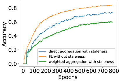
Figure 1: The impact of staleness in AFL

Existing techniques on such conversion, such as DC-ASGD [26], suggested to compensate the errors in stale model updates, but are only applicable to limited amounts of staleness. As shown in Figure 2, when we use the same experiment setting as above and increase the amount of staleness from 0 to 60 epochs, DC-ASGD’s first-order compensation error, measured in cosine similarity and L1-norm difference with the unstale model updates, both significantly increase. The basic reason is that higher-order terms in compensation can not be negligible as staleness becomes large. These results motivate us to further design better techniques that support accurate conversion with unlimited staleness.

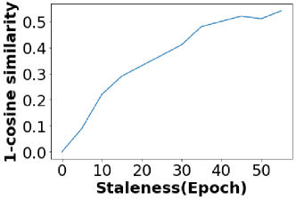
(a) Cosine similarity

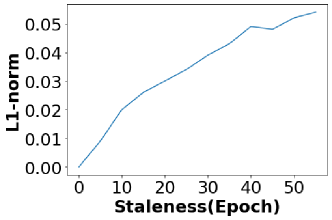
(b) L1-norm difference

Figure 2: DC-ASGD’s compensation error to staleness

2.2 Gradient Inversion

Our proposed approach to addressing the above limitations builds on existing techniques of gradient inversion. Gradient inversion (GI) [29] aims to recover the original training data from gradients of a model under the white box setting, which means that the trained model’s architecture and the setting for training are both known. Its basic idea is to minimize the difference between the trained model’s gradient and the gradient computed from the recovered data. More specifically, denote a batch of training data as $(x,y)$ where $x$ denotes the input data samples and $y$ denotes the corresponding labels, gradient inversion aims to solve the following optimization problem:

$$(x^{\prime*},y^{\prime*})=\arg\min\nolimits_{(x^{\prime},y^{\prime})}\|\frac{\partial L[(x^{\prime},y^{\prime});w^{t-1}]}{\partial w^{t-1}}-g^{t}\|^{2}_{2},\vspace{-0.05in}$$ (1)

where $(x^{\prime},y^{\prime})$ is the recovered data, $w^{t-1}$ is the trained model, $L[\cdot]$ is model’s loss function, and $g^{t}$ is the gradient calculated with the raw training data and $w^{t-1}$. This problem can be solved using gradient descent to iteratively update $(x^{\prime},y^{\prime})$. Since a gradient only contains knowledge from data samples involved in this gradient calculation, gradient inversion can ensure transferring only the relevant knowledge from the training data to the recovered data, achieving higher data quality and minimizing compensation errors.

The quality of recovered data relates to the amount of data samples recovered. Recovering a larger dataset will confuse the knowledge across different data samples, reducing the quality of recovered data. All the existing methods are limited to a small batch ($<$48) of data samples [22; 6; 24]. This limitation contradicts with the typical size of clients’ datasets in FL, calling for alternative ways of better utilizing the recovered data samples.

3 Problem Settings

We consider a FL problem with one server and $N$ clients. At time $t$, a normal client $i$ provides its model update as

$$w^{t}_{i}=LocalUpdate(w^{t}_{global};D_{i}),$$

where $LocalUpdate[\cdot]$ is client $i$’s local training program, which uses the current global model $w^{t}_{global}$ and client $i$’s local dataset $D_{i}$ to produce $w^{t}_{i}$. On the other hand, when the client $i$’s model update is delayed due to either insufficient computing power (i.e., computing delay) or unstable network connection (i.e., communication delay), the server will receive a stale model update from $i$ at time $t$ as

$$w^{t-\tau}_{i}=LocalUpdate(w^{t-\tau}_{global};D_{i}),$$

where the amount of staleness is indicated by $\tau$ and $w^{t-\tau}_{i}$ is computed from an outdated global model $w^{t-\tau}_{global}$.

Due to intertwined data and device heterogeneities, we generally consider that $w^{t-\tau}_{i}$ contains some unique knowledge about $D_{i}$ that is only available from client $i$, and such knowledge needs to be sufficiently incorporated into the current global model. To do so, the server computes an estimation of $w^{t}_{i}$ from the received $w^{t-\tau}_{i}$, namely $\hat{w}^{t}_{i}$, and then uses this estimation in aggregation. During this procedure, the server only receives the stale model update $w^{t-\tau}_{i}$ from client $i$, which does not expose any part of its local dataset $D_{i}$ to the server. The client $i$ does not need to perform any extra computations for such estimation of $\hat{w}^{t}_{i}$, either.

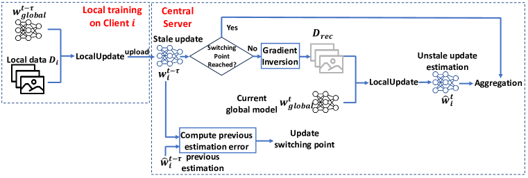
Figure 3: The overall picture of our proposed method of tackling unlimited staleness in FL

4 Methodology

As shown in Figure 3, our proposed technique consists of three key components: 1) recovering an intermediate dataset from the received stale model update via gradient inversion to represent the distribution of the client’s training data; 2) estimating the unstale model update using the recovered dataset; and 3) deciding when to switch back to vanilla FL in the late stage of FL training, to avoid the excessive estimation error from gradient inversion.

4.1 Data Recovery from Stale Model Updates

At time $t$, when the server receives a stale model update $w^{t-\tau}_{i}$ from client $i$ with staleness $\tau$, we adopt gradient inversion described in Eq. (1) into FL, to recover an intermediate dataset $D_{rec}$ from $w^{t-\tau}_{i}$. We expect that $D_{rec}$ represents the similar data distribution with the client $i$’s original training dataset $D_{i}$. To achieve so, we first fix the size of $D_{rec}$ and randomly initialize each data sample and label in $D_{rec}$. Then, we iteratively update $D_{rec}$ by minimizing

$$Disparity[LocalUpdate(w^{t-\tau}_{global};D_{rec}),w^{t-\tau}_{i}],\vspace{-0.05in}$$ (2)

using gradient descent, where $Disparity[\cdot]$ is a metric to evaluate how much $w^{t-\tau}_{i}$ changes if being retrained using $D_{rec}$. In FL, a client’s model update comprises multiple local training steps instead of a single gradient. Hence, to use gradient inversion for data recovery in FL, we substitute the single gradient computed from $D_{rec}$ in Eq. (1) with the local training outcome using $D_{rec}$. In this way, since the loss surface in the model’s weight space computed using $D_{rec}$ is similar to that using $D_{i}$, we can expect a similar gradient being computed. To verify this, we conducted preliminary experiments by using the MNIST dataset to train the LeNet model. Results in Figure 4 show that, the loss surface computed using $D_{rec}$ is highly similar to that using $D_{i}$, in the proximity of the current global model ($w^{t-\tau}_{global}$), and the computed gradient is hence very similar, too.

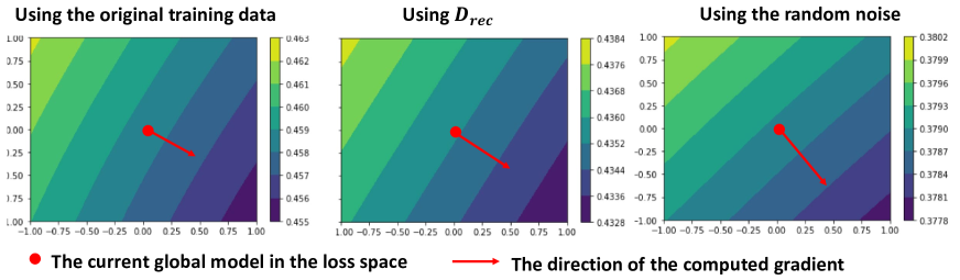
Figure 4: Comparing the loss surface and gradient computed using $D_{rec}$, $D_{i}$, and random noise data

A key issue is how to decide the proper size of $D_{rec}$. Since gradient inversion is equivalent to data resampling in the original training data’s distribution, a sufficiently large size of $D_{rec}$ would be necessary to ensure unbiased data sampling and sufficient minimization of gradient loss through iterations. On the other hand, when the size of $D_{rec}$ is too large, the computational overhead of each iteration would be unnecessarily too high. We experimentally investigated such tradeoff by using the MNIST and CIFAR-10 [10] datasets to train a LeNet model. Results in Tables 1 and 2, where the size of $D_{rec}$ is represented by its ratio to the size of original training data, show that when the size of $D_{rec}$ is larger than 1/2 of the size of the original training data, further increasing the size of $D_{rec}$ only results in little extra reduction of the gradient inversion loss but dramatically increase the computational overhead. Hence, we believe that it is a suitable size of $D_{rec}$ for FL. Considering that clients’ local dataset in FL contain at least hundreds of samples, we expect a big size of $D_{rec}$ in most FL scenarios.

Size	1/64	1/16	1/4	1/2	2	10
Time(s)	193	207	214	219	564	2097
GI loss	27	4.1	2.56	1.74	1.62	1.47

Table 1: Tradeoff between gradient inversion (GI) loss and computing time with different sizes of $D_{rec}$ after 15k iterations, with the MNIST dataset

Size	1/64	1/16	1/4	1/2	2	10
Time(s)	423	440	452	474	1330	4637
GI Loss	1.97	0.29	0.16	0.15	0.15	0.12

Table 2: Tradeoff between gradient inversion (GI) loss and computing time with different sizes of $D_{rec}$ after 15k iterations, with the CIFAR-10 dataset

Such a big size of $D_{rec}$ directly decides our choice of how to evaluate the change of $w^{t-\tau}_{i}$ in Eq. (2). Most existing works use cosine similarity between $LocalUpdate(w^{t-\tau}_{global};D_{rec})$ and $w^{t-\tau}_{i}$ to evaluate their difference in the direction of gradients, so as to maximize the quality of individual data samples in $D_{rec}$ [3]. However, since we aim to recover a large $D_{rec}$, this metric is not applicable, and instead we use L1-norm as the metric to evaluate how using $D_{rec}$ to retrain $w^{t-\tau}_{global}$ will change its magnitude of gradient, to make sure that $D_{rec}$ incurs the minimum impact on the state of training.

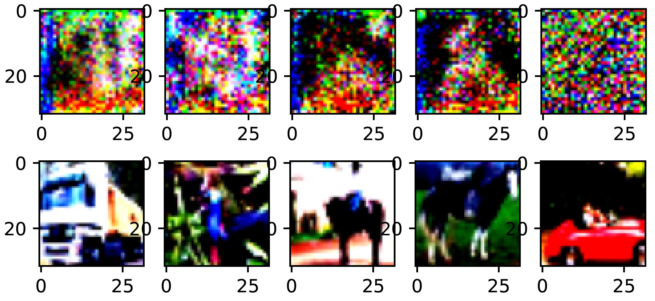
Figure 5: The 5 best matches between samples in $D_{rec}$ and $D_{i}$. The top row represents samples in $D_{rec}$, and the bottom row represents samples in $D_{i}$.

With such a big $D_{rec}$, the similarity between data samples in $D_{rec}$ and $D_{i}$ is the minimum, hence protecting the client $i$’s local data privacy. To verify this, we did experiments with the CIFAR-10 dataset and ResNet-18 model, and match each data sample in $D_{rec}$ with the most similar data sample in $D_{i}$ by computing their LPIPS perceptual similarity score [23]. As shown in Figure 5, these matching data samples are highly dissimilar, and the recovered data samples in $D_{rec}$ are mostly meaningless to humans.

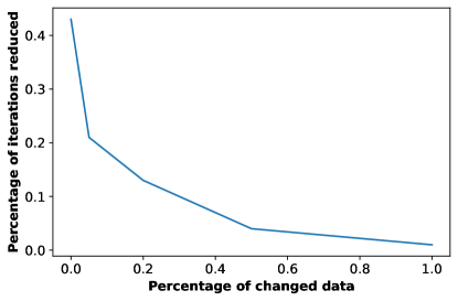
Figure 6: The relationship between reduction in the number of iterations and the percentage of changed data

As shown in Tables 1 and 2, gradient inversion is computationally expensive because it needs a large amount of iterations to converge. In our approach, we reduce this high computational overhead in the following two ways. First, we simplify $LocalUpdate[\cdot]$ in Eq. (2). In the original $LocalUpdate[\cdot]$ used in FL, the client performs training epochs via mini-batch SGD, and a random data augmentation is usually applied to client data before each epoch. To reduce such overhead, in gradient inversion only full-batch gradient descent will be performed. Second, in most FL scenarios, the clients’ local datasets remain fixed, implying that $D_{rec}$ will also be invariant over time. Therefore, instead of starting iterations from a random initialization, we can optimize $D_{rec}$ from those calculated in previous training epochs. In our experiments using the MNIST dataset and the LeNet model, when the client data remains fixed, we observe a reduction in the required iterations in gradient inversion by 43%. When the client data is only partially fixed, Figure 6 that we can still achieve more than 15% reduction when 20% of client data is changing in every epoch.

4.2 Estimating the Unstale Model Updates

Having obtained $D_{rec}$, the server uses it to retrain its current global model to estimate the client $i$’s unstale model update:

$$\hat{w}^{t}_{i}=LocalUpdate[w^{t}_{global};D_{rec}]$$

After that, the server aggregates $\hat{w}^{t}_{i}$ with model updates from other clients, to update its global model in the current epoch.

To verify the accuracy of using $\hat{w}^{t}_{i}$ to estimate $w^{t}_{i}$, we compare this estimation with DC-ASGD’s first-order estimation, by computing their discrepancies with the true unstale model update under different amounts of staleness, using the MNIST dataset and LeNet model. Results in Figure 7 show that, compared to DC-ASGD’s first-order estimation, our estimation based on gradient inversion can reduce the estimation error by up to 50%, especially when the amount of staleness excessively increases to more than 50 epochs.

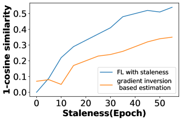
(a) Cosine similarity

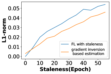
(b) L1-norm difference

Figure 7: Our estimation method has smaller error compared to that of DC-ASGD’s estimation

4.3 Deciding and Updating the Switching Point back to Vanilla FL

As shown in Figure 7, the estimation made by gradient inversion also contains errors, because the gradient inversion loss can not be minimized down to zero. As the FL training goes and the global model converges, the difference between stale and unstale model updates diminishes, implying that the error in our estimated model update ($\hat{w}_{i}^{t}$) will exceed that of the original stale model update $w^{t-\tau}_{i}$ in the late stage of FL training. To verify this, we conducted experiments by training the LeNet model with the MNIST dataset, and evaluated the average values of $E_{1}(t)=Disparity[\hat{w}^{t}_{i};w^{t}_{i}]$ and $E_{2}(t)=Disparity[w^{t-\tau}_{i};w^{t}_{i}]$ across different clients, using both cosine similarity and L1-norm difference as the metric. Results in Figure 8 show that at the final stage of training in FL, $E_{2}(t)$ is always larger than $E_{1}(t)$.

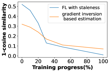
(a) Cosine similarity

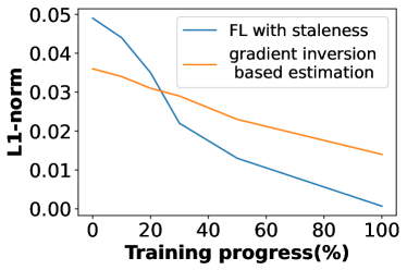
(b) L1-norm difference

Figure 8: Comparison of model updates’ estimation error as the FL training progresses

Hence, in the late stage of FL training, it is necessary to switch back to vanilla FL and directly use stale model updates in aggregation. The difficulty of deciding such switching point is that the true unstale model update ($w^{t}_{i}$) is unknown at time $t$. Instead, the server will be likely to receive $w^{t}_{i}$ at a later time, namely $t+\tau^{\prime}$. Therefore, if we found that $E_{1}(t)>E_{2}(t)$ at time $t+\tau^{\prime}$ when the server receives $w^{t}_{i}$ at $t+\tau^{\prime}$, we can use $t+\tau^{\prime}$ as the switching point instead of $t$. Doing so will result in a delay in switching, but our experiment results in Figure 9 with different switching points show that the FL training is insensitive to such delay.

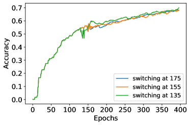
Figure 9: FL training results with different switching points. $E_{1}(t)>E_{2}(t)$ when $t$=155, but different switching points exhibit very similar training performance.

In practice, when we make such switch, the model accuracy in training will experience a sudden drop, as shown in Figure 9, due to the inconsistency of gradient between $\hat{w}^{t}_{i}$ and $w^{t-\tau}_{i}$. To avoid such sudden drop, at time $t+\tau^{\prime}$, instead of immediately switching to using $\hat{w}^{t}_{i}$ in server’s model aggregation, we use a weighted average of $\alpha\hat{w}^{t}_{i}+(1-\alpha)w^{t-\tau}_{i}$ in aggregation, so as to ensure smooth switching.

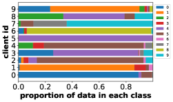
(a) $\alpha$ = 0.1

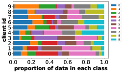
(b) $\alpha$ = 1

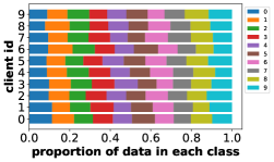
(c) $\alpha$ = 100

Figure 10: Emulating data heterogeneity using the Dirichlet Distribution. Data distributions on 10 clients are shown.

5 Experiments

We evaluated our proposed technique in two FL scenarios. In the first scenario, all clients’ local datasets are fixed. In the second scenario, we consider a more practical FL setting, where clients’ local data is continuously updated and data distributions are variant over time. We believe that the second setting matches the condition of many real-world applications, such as embedded sensing or camera surveillance scenarios, where environmental contexts are changing over time and introducing new knowledge into clients’ local datasets. We compare our proposed technique with the following FL training strategies, and also included the case of FL without any staleness as the baseline in comparison:

• Direct aggregation with staleness: Directly aggregating stale model updates without applying weights onto them.

• Weighted aggregation with staleness: Applying weights onto the stale model updates in aggregation, and these weights generally decay with the amount of staleness [4].

• First-order compensation: Compensating the model update errors caused by staleness using first-order Taylor expansion and Hessian approximation as described in DC-ASGD [26].

5.1 Experiment Setup

In all experiments, we consider a FL scenario with 100 clients. Each local model update on a client is trained by 5 epochs using the SGD optimizer, with a learning rate of 0.01 and momentum of 0.5.

To emulate data heterogeneity, we use a Dirichlet distribution to sample client datasets with different label distributions [7], and use a tunable parameter ($\alpha$) to adjust the amount of data heterogeneity: as shown in Figure 10, the smaller $\alpha$ is, the more biased these label distributions will be and hence the higher amount of data heterogeneity exists. When $\alpha$ is very small, the local dataset of each client only contains data samples of few data classes.

To emulate device heterogeneity intertwined with data heterogeneity, we select one data class to be affected by staleness, and apply different amounts of staleness, measured by the number of epochs that the clients’ model updates are delayed, to the top 10 clients whose local datasets contain the most data samples of the selected data class. The impact of staleness, on the other hand, can be further enlarged by applying staleness in the similar way to more data classes.

Based on such experiment setup, in all experiments, we assess our approach’s performance improvement by measuring the increase of model accuracy in the selected data class being affected by staleness. We expect that our approach can either improve the final model accuracy when the training completes, or achieve the same level of model accuracy with the existing methods but use fewer training epochs.

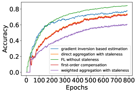
Figure 11: Model accuracy in data class 5 affected by staleness, using MNIST dataset to train a LeNet model

5.2 FL Performance in the Fixed Data Scenario

In the fixed data scenario, we conduct experiments in two FL settings: 1) the MNIST [11] dataset to train a LeNet model and 2) the CIFAR-10 [10] dataset to train a ResNet-8 model.

When staleness is 40 epochs, Figure 11 and 12 show that our proposed technique results in much better model accuracy in both FL settings. At the early stage of FL, the model accuracy achieved by our technique of gradient inversion based model estimation is very close to that of FL without staleness, indicating that our technique can fully remove the impact of staleness. In contrast, directly aggregating stale model updates could result in 7.5% drop in model accuracy, and using weighted aggregation with staleness could even increase such model accuracy drop to up to 20%.

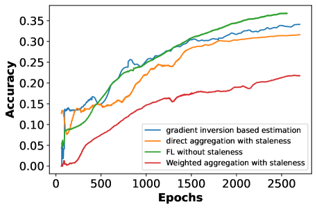
Figure 12: Model accuracy in data class 2 affected by staleness, using CIFAR-10 dataset to train a ResNet-8 model

Our technique can also greatly speed up the training progress. As shown in Figure 11 and 12, compared to direct aggregation or weighted aggregation with staleness, to achieve the same model accuracy in the early stage of training (before 400 epochs in Figure 11 and before 1000 epochs in Figure 12), our technique can reduce the required training time by 27.5% and 35%, for the MNIST and CIFAR-10 dataset, respectively. This speedup is particularly important in many time-sensitive and mission-critical applications such as embedded sensing, where coarse-grained but fast model ability is needed.

training time accuracy	Staleness (epoch)
	10	20	40
GI-based Estimation	720	660	580
	73.3%	75.2%	77.7%
Direct Aggregation	800	800	800
	72.6%	73.1%	73.9%
First Order compensation	790	780	820
	72.8%	73.1%	73.7%

Table 3: The trained model accuracy and amount of training time spent with different amounts of staleness, measured in the number of delayed epochs

training time accuracy	$\alpha$
	100	1	0.1
GI-based Estimation	800	760	580
	82.3%	78.1%	78.3%
Direct Aggregation	800	800	800
	82.3%	77.2%	73.2%
First Order compensation	800	800	820
	82.3%	77.2%	72.7%

Table 4: The trained model accuracy and amount of training time spent with different amounts of data heterogeneity, controlled by the tunable parameter $\alpha$)

Furthermore, we also conducted experiments with different amounts of data heterogeneity and device heterogeneity (a.k.a., staleness) using the MNIST dataset and the LeNet model. Results in Tables 3 and 4 show that, compared with the existing schemes including direct aggregation and first-order compensation, our proposed gradient inversion (GI)-based estimation can generally achieve higher model accuracy using a smaller amount of training epochs. Especially when the amount of staleness increases to a unlimited level (e.g., 20-40 epochs) or the data distributions among different clients are highly heterogeneous, the improvement of model accuracy could be up to 5% with $>$30% less training epochs. These results demonstrate that our proposed method can be widely applied to different FL scenarios with unlimited amount of staleness and data heterogeneity.

5.3 FL Performance in the Variant Data Scenario

To continuously vary the data distributions of clients’ local datasets, we use two public datasets, namely MNIST and SVHN [15], which are for the same learning task (i.e., handwriting digit recognition) but with different feature representations as shown in Figure 13. Each client’s local dataset is initialized as the MNIST dataset in the same way as in the fixed data scenario. Afterwards, during training, each client continuously replaces random data samples in its local dataset with new data samples in the SVHN dataset.

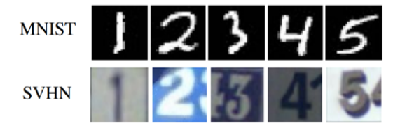
Figure 13: Datasets for digit recognition: MNIST and SVHN

Experiment results in Figure 14 show that in such variant data scenario, since clients’ local data distributions continuously change, the FL training will never converge. Hence, the model accuracy improvements by the existing FL training strategies, including both direct aggregation with staleness and first-order compensation, exhibit significant fluctuations over time and stay low ($<$40%). In comparison, our proposed gradient inversion based estimation can better depict the variant data patterns and hence achieve much higher model accuracy, which is comparable to FL without staleness and 20% higher than those in existing FL schemes.

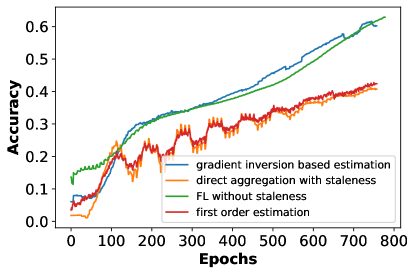
Figure 14: Model accuracy with variant data distributions in clients’ local datasets

In addition, we also conducted experiments with different amounts of staleness and rates of data variation. Results in Tables 5 and 6 demonstrated that our proposed method outperformed the existing FL strategies in different scenarios with different dynamics of local data patterns.

training time accuracy	Staleness (epoch)
	10	20	40
GI-based Estimation	760	710	440
	54.0%	52.4%	60.2%
Direct Aggregation	800	800	800
	51.4%	46.6%	40.7%
First Order compensation	800	800	820
	51.4%	46.5%	40.9%

Table 5: The trained model accuracy and amount of training time spent with different amounts of staleness

training time accuracy	streaming rate
	1/4	1/3	1/2
GI-based Estimation	330	330	440
	32.2%	41.9%	60.2%
Direct Aggregation	800	800	800
	27.8%	32.6%	40.7%
First Oreder Compensation	830	800	820
	27.5%	32.6%	40.9%

Table 6: Model accuracy and amount of training time with different rates of clients’ data variation, measured as the number of local data samples being replaced in each epoch (e.g., 1/2 is to replace one data sample every 2 epochs)

6 Related Work

Staleness in asynchronous FL (AFL): Most existing solutions to staleness in AFL are based on weighted aggregation. For example, [4] suggests that a model update’s weight exponentially decays with its amount of staleness, and some others use different staleness metrics to decide model updates’ weights [17]. [5] decides these weights based on a feature learning algorithm. These existing solutions are always biased towards fast clients, and will hence affect the trained model’s accuracy when data and device heterogeneities in FL are intertwined. Some other researchers suggest to use semi-asynchronous FL, where the server either aggregates client model updates at a lower frequency [16] or clusters clients into different asynchronous “tiers” according to their update rates [2]. However, doing so cannot completely eliminate the impact of staleness because the server’s aggregation still involves stale model updates.

Recovering training data: We can recover the training data from stale model updates and use the recovered data to transfer knowledge from stale model updates to the global model. Such recovery can be done by training a generative model and compelling its generated data to exhibit high predictive values on the original model [20; 12; 30]. Another approach is to directly optimize the randomly initialized input data until it has good performance on the original model [21]. However, the quality of recovered data from these methods remains low. Other efforts enhance data quality by incorporating natural image priors [13] or using another public dataset to introduce general knowledge [19], but require involvement of extra datasets. Moreover, all these methods require that the original model update to be fully trained, which is usually infeasible in FL.

7 Conclusion

In this paper, we present a new FL framework to tackle the unlimited staleness when data and device heterogeneities are intertwined, by using gradient inversion to compute non-stale model updates from clients’ stale model updates. Experiment results show that our technique can largely improve the model accuracy and speed up FL training.

References

- Acar et al. [2021] D. A. E. Acar, Y. Zhao, R. M. Navarro, M. Mattina, P. N. Whatmough, and V. Saligrama. Federated learning based on dynamic regularization. arXiv preprint arXiv:2111.04263, 2021.
- Chai et al. [2021] Z. Chai, Y. Chen, A. Anwar, L. Zhao, Y. Cheng, and H. Rangwala. Fedat: A high-performance and communication-efficient federated learning system with asynchronous tiers. In Proceedings of the International Conference for High Performance Computing, Networking, Storage and Analysis, pages 1–16, 2021.
- Charpiat et al. [2019] G. Charpiat, N. Girard, L. Felardos, and Y. Tarabalka. Input similarity from the neural network perspective. Advances in Neural Information Processing Systems, 32, 2019.
- Chen et al. [2019] Y. Chen, X. Sun, and Y. Jin. Communication-efficient federated deep learning with layerwise asynchronous model update and temporally weighted aggregation. IEEE transactions on neural networks and learning systems, 31(10):4229–4238, 2019.
- Chen et al. [2020] Y. Chen, Y. Ning, M. Slawski, and H. Rangwala. Asynchronous online federated learning for edge devices with non-iid data. In 2020 IEEE International Conference on Big Data (Big Data), pages 15–24. IEEE, 2020.
- Geiping et al. [2020] J. Geiping, H. Bauermeister, H. Dröge, and M. Moeller. Inverting gradients-how easy is it to break privacy in federated learning? Advances in Neural Information Processing Systems, 33:16937–16947, 2020.
- Hsu et al. [2019] T.-M. H. Hsu, H. Qi, and M. Brown. Measuring the effects of non-identical data distribution for federated visual classification. arXiv preprint arXiv:1909.06335, 2019.
- Karimireddy et al. [2020] S. P. Karimireddy, S. Kale, M. Mohri, S. Reddi, S. Stich, and A. T. Suresh. Scaffold: Stochastic controlled averaging for federated learning. In International conference on machine learning, pages 5132–5143. PMLR, 2020.
- Konečnỳ et al. [2016] J. Konečnỳ, H. B. McMahan, D. Ramage, and P. Richtárik. Federated optimization: Distributed machine learning for on-device intelligence. arXiv preprint arXiv:1610.02527, 2016.
- Krizhevsky [2009] a. G. H. Krizhevsky, Alex. Learning multiple layers of features from tiny images. 2009.
- LeCun and Burges. [2010] C. C. LeCun, Yann and C. Burges. Mnist handwritten digit database. http://yann.lecun.com/exdb/mnist, 2010.
- Lopes et al. [2017] R. G. Lopes, S. Fenu, and T. Starner. Data-free knowledge distillation for deep neural networks. arXiv preprint arXiv:1710.07535, 2017.
- Luo et al. [2020] L. Luo, M. Sandler, Z. Lin, A. Zhmoginov, and A. Howard. Large-scale generative data-free distillation. arXiv preprint arXiv:2012.05578, 2020.
- McMahan et al. [2017] B. McMahan, E. Moore, D. Ramage, S. Hampson, and B. A. y Arcas. Communication-efficient learning of deep networks from decentralized data. In Artificial intelligence and statistics, pages 1273–1282. PMLR, 2017.
- Netzer et al. [2011] Y. Netzer, T. Wang, A. Coates, A. Bissacco, B. Wu, and A. Y. Ng. Reading digits in natural images with unsupervised feature learning. 2011.
- Nguyen et al. [2022] J. Nguyen, K. Malik, H. Zhan, A. Yousefpour, M. Rabbat, M. Malek, and D. Huba. Federated learning with buffered asynchronous aggregation. In International Conference on Artificial Intelligence and Statistics, pages 3581–3607. PMLR, 2022.
- Wang et al. [2022] Q. Wang, Q. Yang, S. He, Z. Shi, and J. Chen. Asyncfeded: Asynchronous federated learning with euclidean distance based adaptive weight aggregation. arXiv preprint arXiv:2205.13797, 2022.
- Xie et al. [2019] C. Xie, S. Koyejo, and I. Gupta. Asynchronous federated optimization. arXiv preprint arXiv:1903.03934, 2019.
- Yang et al. [2019] Z. Yang, J. Zhang, E.-C. Chang, and Z. Liang. Neural network inversion in adversarial setting via background knowledge alignment. In Proceedings of the 2019 ACM SIGSAC Conference on Computer and Communications Security, pages 225–240, 2019.
- Ye et al. [2020] J. Ye, Y. Ji, X. Wang, X. Gao, and M. Song. Data-free knowledge amalgamation via group-stack dual-gan. In Proceedings of the IEEE/CVF Conference on Computer Vision and Pattern Recognition, pages 12516–12525, 2020.
- Yin et al. [2020] H. Yin, P. Molchanov, J. M. Alvarez, Z. Li, A. Mallya, D. Hoiem, N. K. Jha, and J. Kautz. Dreaming to distill: Data-free knowledge transfer via deepinversion. In Proceedings of the IEEE/CVF Conference on Computer Vision and Pattern Recognition, pages 8715–8724, 2020.
- Yin et al. [2021] H. Yin, A. Mallya, A. Vahdat, J. M. Alvarez, J. Kautz, and P. Molchanov. See through gradients: Image batch recovery via gradinversion. In Proceedings of the IEEE/CVF Conference on Computer Vision and Pattern Recognition, pages 16337–16346, 2021.
- Zhang et al. [2018] R. Zhang, P. Isola, A. A. Efros, E. Shechtman, and O. Wang. The unreasonable effectiveness of deep features as a perceptual metric. In Proceedings of the IEEE conference on computer vision and pattern recognition, pages 586–595, 2018.
- Zhao et al. [2020] B. Zhao, K. R. Mopuri, and H. Bilen. idlg: Improved deep leakage from gradients. arXiv preprint arXiv:2001.02610, 2020.
- Zhao et al. [2018] Y. Zhao, M. Li, L. Lai, N. Suda, D. Civin, and V. Chandra. Federated learning with non-iid data. arXiv preprint arXiv:1806.00582, 2018.
- Zheng et al. [2017] S. Zheng, Q. Meng, T. Wang, W. Chen, N. Yu, Z.-M. Ma, and T.-Y. Liu. Asynchronous stochastic gradient descent with delay compensation. In International Conference on Machine Learning, pages 4120–4129. PMLR, 2017.
- Zhou et al. [2021a] C. Zhou, H. Tian, H. Zhang, J. Zhang, M. Dong, and J. Jia. Tea-fed: time-efficient asynchronous federated learning for edge computing. In Proceedings of the 18th ACM International Conference on Computing Frontiers, pages 30–37, 2021a.
- Zhou et al. [2021b] Y. Zhou, Q. Ye, and J. Lv. Communication-efficient federated learning with compensated overlap-fedavg. IEEE Transactions on Parallel and Distributed Systems, 33(1):192–205, 2021b.
- Zhu et al. [2019] L. Zhu, Z. Liu, and S. Han. Deep leakage from gradients. Advances in neural information processing systems, 32, 2019.
- Zhu et al. [2021] Z. Zhu, J. Hong, and J. Zhou. Data-free knowledge distillation for heterogeneous federated learning. In International conference on machine learning, pages 12878–12889. PMLR, 2021.