Robust Principal Component Analysis using Density Power Divergence

Abstract

Principal component analysis (PCA) is a widely employed statistical tool used primarily for dimensionality reduction. However, it is known to be adversely affected by the presence of outlying observations in the sample, which is quite common. Robust PCA methods using M-estimators have theoretical benefits, but their robustness drop substantially for high dimensional data. On the other end of the spectrum, robust PCA algorithms solving principal component pursuit or similar optimization problems have high breakdown, but lack theoretical richness and demand high computational power compared to the M-estimators. We introduce a novel robust PCA estimator based on the minimum density power divergence estimator. This combines the theoretical strength of the M-estimators and the minimum divergence estimators with a high breakdown guarantee regardless of data dimension. We present a computationally efficient algorithm for this estimate. Our theoretical findings are supported by extensive simulations and comparisons with existing robust PCA methods. We also showcase the proposed algorithm’s applicability on two benchmark datasets and a credit card transactions dataset for fraud detection.

Keywords: Robust PCA, Eigen Decomposition, Matrix Factorization, Density Power Divergence, Breakdown Point

1 Introduction

The classical problem of finding the principal components aims to approximate the covariance structure of a high dimensional sample of many features by the covariance structure of a lower dimensional sample of “principal components”, obtained as linear combinations of the original feature variables. Mathematically, starting with an independent and identically distributed (i.i.d.) sample $\boldsymbol{X}_{1},\boldsymbol{X}_{2},\dots\boldsymbol{X}_{n}$, where each $\boldsymbol{X}_{i}\in\mathbb{R}^{p}$, and a scale measure $S_{n}(y_{1},\dots y_{n})$ to measure the dispersion in a univariate sample $\{y_{1},\dots y_{n}\}$, the first eigenvector associated with the principal components is defined as the unit length vector maximizing the function

$$\boldsymbol{v}\rightarrow S_{n}(\boldsymbol{v}^{\intercal}\boldsymbol{X}_{1},\dots\boldsymbol{v}^{\intercal}\boldsymbol{X}_{n});\ \boldsymbol{v}\in\mathbb{R}^{p}.$$ (1.1)

Similarly, assuming that the first $(k-1)$ eigenvectors $\widehat{\boldsymbol{v}}_{1},\widehat{\boldsymbol{v}}_{2},\dots\widehat{\boldsymbol{v}}_{k-1}$ has already been found, one can obtain the subsequent $k$-th eigenvector as the unit vector maximizing the same function given in Eq. (1.1), but under the set of restrictions $\boldsymbol{v}^{\intercal}\widehat{\boldsymbol{v}}_{i}=0$ for all $i=1,\dots(k-1)$. The corresponding eigenvalues are defined as the maximum values of the scale function, i.e.,

$$\widehat{\lambda}_{k}=S_{n}(\widehat{\boldsymbol{v}}_{k}^{\intercal}\boldsymbol{X}_{1},\dots\widehat{\boldsymbol{v}}_{k}^{\intercal}\boldsymbol{X}_{n}).$$

In essence, principal component analysis (PCA) takes input $n$ observations of dimension $p$, where $p$ is presumably very large, and outputs a set of pairs $\{(\widehat{\lambda}_{k},\widehat{\boldsymbol{v}}_{k}):k=1,2,\dots r\}$ where $r$ is a pre-specified number of components, generally much smaller compared to both $n$ and $p$. For each $k$, the former of the pair $\widehat{\lambda}_{k}$ denotes the maximum variability expressed by the $k$-th principal component, and the latter of the pair $\widehat{\boldsymbol{v}}_{k}$ denotes the direction along which this maximum variability can be found in the given i.i.d. sample. The $k$-th principal component is then defined by the variable obtained from projecting the observations along the $k$-th eigenvector scaled by the $k$-th eigenvalue, i.e., $\{\widehat{\lambda}_{k}\widehat{\boldsymbol{v}}_{k}^{\intercal}\boldsymbol{X}_{i}:i=1,\dots n\}$.

Since a small number of principal components can explain most of the variation present in the random sample, it is primarily used for the purpose of dimensionality reduction. PCA provides a simple method of visualizing any high-dimensional data by plotting the first two or three principal components, and subsequently one can identify potential outliers [Locantore et al., 1999]. Jolliffe [2002] also provides an application of PCA for variable selection in the regression context. In machine learning and pattern recognition, PCA has been used abundantly for both supervised and unsupervised paradigms [Vathy-Fogarassy and Abonyi, 2013]. PCA has also found its applications across many disciplines ranging from multi-sensor data fusion [Lock et al., 2013], signal processing, image compression [Bouwmans et al., 2018], video event detection [Roy et al., 2021] to material and chemical sciences [Smilde et al., 2005]. The readers are referred to see Sanguansat [2012] and the references therein for further details on the multitude of applications of PCA.

In the classical PCA, the scale estimator $S_{n}(y_{1},y_{2},\dots y_{n})$ is chosen to be the square root of the sample variance. As a result, the eigenvalues and the eigenvectors of the sample covariance matrix of $\boldsymbol{X}_{1},\dots\boldsymbol{X}_{n}$ become the solution to the aforementioned principal components problem. It is well known that the sample covariance matrix is very sensitive to outliers, hence the principal components resulting from classical PCA also suffer from the presence of outlying observations in the data [Hubert et al., 2005, Candès et al., 2011]. In the context of the high dimensional datasets pertaining to the above applications, it is very challenging to locate these outlying observations beforehand in order to discard them. Thus, any practitioner relying solely on the classical PCA to interpret multivariate data may end up with a distorted visualization of the data, false detection of outliers, and a wrong conclusion about the data. Several robustified versions of PCA have been proposed to date to provide reliable estimates of the principal components even under the presence of outlying observations [Jolliffe, 2002]. A brief discussion of the existing literature in this area is provided in the following subsection.

1.1 Existing Literature

Most of the early literature to derive a robust principal component analysis (RPCA) followed one of the two primary approaches. The first class of estimators estimated the principal components robustly from the eigenvalues and the eigenvectors of a robust covariance matrix of the sample. Notable among this class of estimators are those due to Maronna [1976] and Campbell [1980], where the authors create affine-equivariant principal component estimates from robust M-estimators of the covariance matrix. Devlin et al. [1981] proposed to use minimum covariance determinant (MCD) estimator and minimum volume ellipsoid (MVE) estimator [Rousseeuw, 1985] for this purpose due to their high breakdown compared to the M-estimators.

The other approach considered robustifying PCA by using a robust scale function $S_{n}$ in Eq. (1.1). This idea was first presented by Li and Chen [1985] and was further developed later by Croux and Ruiz-Gazen [1996] where they considered the median absolute deviation about sample median as the scale function. Various theoretical properties like the influence function, asymptotic distribution and the breakdown point of this estimator have also been established in the literature [Croux and Haesbroeck, 2000, Croux and Ruiz-Gazen, 2005]. These estimators and their variants primarily restricted their attention to the elliptically symmetric family of distributional models, i.e., the random observations $\boldsymbol{X}_{i}$ for $i=1,2\dots n$ were assumed to follow a density function of the form

$$f(\boldsymbol{x})\propto g\left((\boldsymbol{x}-\boldsymbol{\mu})^{\intercal}\boldsymbol{\Sigma}^{-1}(\boldsymbol{x}-\boldsymbol{\mu})\right),$$ (1.2)

where $g:\mathbb{R}^{+}\rightarrow\mathbb{R}$ is a known function governing the shape of the density. It turns out that under this model, $\mathbb{E}(\boldsymbol{X}_{i})=\boldsymbol{\mu}$ and $\mathbb{E}\left((\boldsymbol{X}_{i}-\boldsymbol{\mu})(\boldsymbol{X}_{i}-\boldsymbol{\mu})^{\intercal}\right)=\boldsymbol{\Sigma}$ (Based on the usual notation for elliptically symmetric family, the variance of $\boldsymbol{X}_{i}$ is $k_{g}\boldsymbol{\Sigma}$ where $k_{g}$ is a constant depending on the function $g$, but we assume that such $k_{g}$ is included in the dispersion matrix $\boldsymbol{\Sigma}$ itself by modifying the function $g$ appropriately). Even though these statistical RPCA approaches guarantee the highest possible asymptotic breakdown point of $1/2$, they show low asymptotic efficiency and sometimes large bias even at considerably lower levels of contaminations than their breakdowns [Fishbone and Mili, 2023].

Recent advances in the area of RPCA view the estimation of the principal components in a different light through the guise of the factor model. Wright et al. [2009] define the RPCA problem as the problem of recovering $\boldsymbol{L}$ from the unknown decomposition of the data matrix $\boldsymbol{X}=\boldsymbol{L}+\boldsymbol{S}$, where $\boldsymbol{L}$ is a low rank matrix and $\boldsymbol{S}$ is a sparse noise component. The direct solution to this problem would consider the optimization problem

$$\min_{\boldsymbol{L},\boldsymbol{S}}\text{Rank}\left(\boldsymbol{L}\right)+\gamma\|\boldsymbol{S}\|_{0},$$ (1.3)

subject to the restriction that $\|\boldsymbol{S}\|_{0}\leq k$ and $\boldsymbol{X}=\boldsymbol{L}+\boldsymbol{S}$, for a predetermined value of $k$. Here, $\|\boldsymbol{A}\|_{0}$ denotes the $L_{0}$-norm of the matrix $\boldsymbol{A}$, i.e., the sum of the nonzero entries of $\boldsymbol{A}$ and $\gamma$ is a tuning parameter to control the balance between the rank of $\boldsymbol{L}$ and the sparsity of $\boldsymbol{S}$. As noted in Candès et al. [2011], the classical PCA seeks the best low-rank component $\boldsymbol{L}$ in terms of minimizing the usual Euclidean $L_{2}$ norm, i.e., it is related to the optimization problem $\min_{\boldsymbol{L}}\|\boldsymbol{X}-\boldsymbol{L}\|_{2}$ subject to the restriction that $\text{Rank}\left(\boldsymbol{L}\right)\leq k$. However, the problem in Eq. (1.3) is notoriously difficult to solve, hence Wright et al. [2009] and Candès et al. [2011] considered the convex optimization problem $\min_{\boldsymbol{L},\boldsymbol{S}}\|\boldsymbol{L}\|_{\ast}+\gamma\|\boldsymbol{S}\|_{1}$ where $\|\boldsymbol{L}\|_{\ast}$ is the nuclear norm of the matrix $\boldsymbol{L}$, i.e., the sum of its singular values and $\|\boldsymbol{S}\|_{1}$ is the $L_{1}$ norm of the matrix $\boldsymbol{S}$. Various algorithmic techniques like principal component pursuit (PCP) method [Candès et al., 2011], augmented Lagrange multiplier (ALM) method [Lin et al., 2010] and alternating projection (AltProj) algorithm [Cai et al., 2019] have been developed to solve this optimization problem efficiently. This new approach radically differs from the traditional statistical methods: these methods are non-parametric in nature and assume that the data matrix $\boldsymbol{X}$ is non-stochastic, rather the only source of randomness comes from the positions of the nonzero entries of the sparse matrix $\boldsymbol{S}$. The convergence and correctness guarantees of these methods are then provided based on the bounds on the entries of these matrices $\boldsymbol{L}$ and $\boldsymbol{S}$ directly. This exact decomposition is often far from practical applications as every entry of the data matrix $\boldsymbol{X}$ is subject to measurement errors. To mitigate this, Zhou et al. [2010] considered the decomposition

$$\boldsymbol{X}=\boldsymbol{L}+\boldsymbol{S}+\boldsymbol{E},$$ (1.4)

where $\boldsymbol{E}$ is a dense perturbation matrix (such as matrix with i.i.d. mean zero and homoscadastic entries). Although such a decomposition is considered, the analysis of the algorithm still assumed $\boldsymbol{X}$ to be deterministic and considered $\|\boldsymbol{E}\|_{2}\leq\delta$, a prespecified level of noise variance to maintain a high signal-to-noise ratio.

1.2 Connection between RPCA Approaches and Our Contributions

The two existing RPCA approaches, one based on the maximization of the scale function as in Eq. (1.1) and another based on the minimization of objective function Eq. (1.3) with matrix decomposition, are usually not equivalent except for the trivial cases of classical PCA. In this paper, we consider a combination of both approaches by taking the decomposition given in Eq. (1.4) but with stochastic modelling of the data matrix $\boldsymbol{X}$. We assume that the rows of the data matrix $\boldsymbol{X}$, namely $\boldsymbol{X}_{1},\dots\boldsymbol{X}_{n}$ are i.i.d. observations generated from an elliptically symmetric family of distributions having a density function of the form as in Eq. (1.2). Clearly, the sample observations can be expressed as $\boldsymbol{X}_{i}=\boldsymbol{\mu}+\boldsymbol{\Sigma}^{1/2}\boldsymbol{Z}_{i}$, for $i=1,2,\dots n$, where $\boldsymbol{Z}_{i}$ are i.i.d. random variables with $\mathbb{E}(\boldsymbol{Z}_{i})=0$ and $\mathbb{E}(\boldsymbol{Z}_{i}\boldsymbol{Z}_{i}^{\intercal})=\boldsymbol{I}_{p}$, the identity matrix of order $p$. The density function of the random variable $\boldsymbol{Z}_{i}$ depends on the specific form of the $g$ function. Then, incorporating the eigendecomposition of $\boldsymbol{\Sigma}=\sum_{k=1}^{p}\gamma_{k}\boldsymbol{v}_{k}\boldsymbol{v}_{k}^{\intercal}$ (with $\gamma_{1}\geq\gamma_{2}\dots\geq\gamma_{p}$), we can rewrite the data matrix as

$$\boldsymbol{X}=\boldsymbol{1}_{n}\boldsymbol{\mu}^{\intercal}+\sum_{k=1}^{p}\sqrt{\gamma_{k}}\boldsymbol{Z}\boldsymbol{v}_{k}\boldsymbol{v}_{k}^{\intercal},$$ (1.5)

where $\boldsymbol{1}_{n}$ denotes the $n$-length column vector with all elements equal to $1$ and $\boldsymbol{Z}$ is the $n\times p$ matrix whose $i$-th row is equal to $\boldsymbol{Z}_{i}^{\intercal}$. Denoting $\boldsymbol{u}_{k}=\boldsymbol{Z}\boldsymbol{v}_{k}/\sqrt{n}$ for $k=1,2,\dots p$, one can easily see that $\boldsymbol{u}_{k}$s form a set of orthonormal vectors in expectation, i.e., $\mathbb{E}(\boldsymbol{u}_{k}^{\intercal}\boldsymbol{u}_{l})=\delta_{kl}$, the Kronecker delta function. This enables us to rewrite Eq. (1.5) as

$$\boldsymbol{X}=\boldsymbol{1}_{n}\boldsymbol{\mu}^{\intercal}+\sum_{k=1}^{r}\sqrt{n\gamma_{k}}\boldsymbol{u}_{k}\boldsymbol{v}_{k}^{\intercal}+\sum_{k=(r+1)}^{p}\sqrt{n\gamma_{k}}\boldsymbol{u}_{k}\boldsymbol{v}_{k}^{\intercal},$$ (1.6)

for some prespecified rank $r$. Ignoring the location, the rest of the decomposition is $\boldsymbol{X}=\boldsymbol{L}+\boldsymbol{E}$ which is a subset of the model given in Eq. (1.4) without any sparse component. In the presence of outlying observations in the data matrix $\boldsymbol{X}$, the resulting error matrix $\boldsymbol{E}$ will contain occasional spikes which can be separated into the sparse component $\boldsymbol{S}$ giving rise to the decomposition in Eq. (1.4). Connecting the low rank matrix $\boldsymbol{L}$ in Eq. (1.4) to the sum $\sum_{k=1}^{r}\sqrt{n\gamma_{k}}\boldsymbol{u}_{k}\boldsymbol{v}_{k}^{\intercal}$ in Eq. (1.6), it is now evident that maximizing the scale function of Eq. (1.1) would result in the eigenvectors $\boldsymbol{v}_{k}$s which are the right singular vectors of the $\boldsymbol{L}$ matrix. This provides a connection between the two approaches when the rows of the data matrix are i.i.d. observations from an elliptically symmetric family of distributions. Thus, in this paper, we propose a fast, scalable novel robust PCA algorithm based on the popular minimum density power divergence estimation (MDPDE) approach [Basu et al., 1998] for the aforementioned setup along with a decomposition as in Eq. (1.6). The major contributions of this paper are as follows:

1. We propose a novel robust PCA estimator (to be henceforth called rPCAdpd) based on the popular MDPDE, which allows balancing the robustness and efficiency in estimation by simply tuning a robustness parameter $\alpha$ and is able to work under a general decomposition model as in Eq. (1.4).

2. We propose a fast, parallelizable iterative algorithm to obtain the rPCAdpd estimate based on alternating regression; this contrasts with the existing robust PCA algorithms which do not scale well due to large matrix inversion steps.

3. We also derive various theoretical properties such as equivariance, $\sqrt{n}$-consistency and asymptotic distribution of the proposed rPCAdpd estimator akin to the widely used robust M-estimators. There exists little literature on the theoretical behaviour of the existing PCP methods and often the asymptotic distributions of these estimators are non-Gaussian [Bickel et al., 2018].

4. We also theoretically demonstrate the robustness of the proposed rPCAdpd estimator by demonstrating that its influence function is bounded, and by deriving a lower bound of its asymptotic breakdown point which is independent of the data dimension $p$ but only a function of the robustness tuning parameter $\alpha$. This ensures the scalability of the proposed rPCAdpd estimator for arbitrarily high dimensional random samples.

5. We corroborate our theoretical findings with extensive simulations. For all the simulation setups considered, rPCAdpd performs better (and sometimes closely on par) than the existing RPCA algorithms.

6. We also compare the performances of the existing robust PCA algorithms with the rPCAdpd for a few benchmark datasets, and demonstrate how the estimator can be used to detect fraudulent transactions for a credit card transactions dataset.

The rest of the paper is structured as follows: our proposed rPCAdpd estimator is described in detail in Section 2.1 when the model family is elliptically symmetric. In Section 2.2, we derive a computationally efficient iterative technique to obtain the rPCAdpd estimator using the solution to an alternating regression problem. Section 3 describes the necessary theoretical results regarding the convergence of the algorithm, equivariance properties, consistency and asymptotic distribution of the estimator. All of these theoretical results are then corroborated by extensive simulation studies in Section 4, where we compare the performance of the rPCAdpd estimator with several existing robust PCA algorithms. Finally, in Section 5, we demonstrate the practical applicability of the proposed estimator for two popular benchmark datasets (namely the Car dataset and Octane dataset in Hubert et al. [2005]) and a Credit Card Fraud Detection dataset. For streamlining the presentation, the proofs of all of the theoretical results are deferred till the Appendix.

2 The rPCAdpd Estimator

Before proceeding with the description of the proposed rPCAdpd estimator, we introduce some notations to be used throughout the paper unless otherwise specified. Let, for a matrix $\boldsymbol{A}$, $\text{Diag}\left(\boldsymbol{A}\right)$ denote the vector comprising the diagonal elements of $\boldsymbol{A}$. The notations $\boldsymbol{I}_{n}$ and $\boldsymbol{1}_{n}$ denote the $n\times n$-size identity matrix and $n$-length vector of $1$s respectively. The transpose, rank and the trace of a matrix $\boldsymbol{A}$ will be denoted as $\boldsymbol{A}^{\intercal}$, $\text{Rank}\left(\boldsymbol{A}\right)$ and $\text{Trace}\left(\boldsymbol{A}\right)$. For any two matrices $\boldsymbol{A}$ and $\boldsymbol{B}$, their usual matrix product will be denoted as $\boldsymbol{A}\boldsymbol{B}$ and the Kronecker product will be denoted as $\boldsymbol{A}\otimes\boldsymbol{B}$. We shall use the symbol $\|\boldsymbol{x}\|_{2}$ and $\|\boldsymbol{A}\|_{2}$ to denote the usual Euclidean norm of a vector $\boldsymbol{x}$ and the Frobenius norm of the matrix $\boldsymbol{A}$ respectively. The notation $f_{\boldsymbol{\theta}}(\boldsymbol{x})$ will denote a generic symbol of the probability density function of a random variable $\boldsymbol{X}$ following a distribution parametrized by $\boldsymbol{\theta}$ and evaluated at a point $\boldsymbol{x}$. The expectation and the covariance operator will be denoted by $\mathbb{E}(\cdot)$ and $\mathrm{Var}(\cdot)$ respectively.

2.1 Description of the rPCAdpd Estimator

Let $\boldsymbol{X}_{1},\dots\boldsymbol{X}_{n}$ be a $p$-variate sample such that each of the observations $\boldsymbol{X}_{i}$ follows an elliptically symmetric family of distributions with a density function of the form

$$f_{\boldsymbol{\theta}}(\boldsymbol{x})=c_{g}^{-1}\det(\boldsymbol{\Sigma})^{-1/2}\exp\left[g\left(\boldsymbol{x}^{\intercal}\sum_{k=1}^{p}\gamma_{k}^{-1}\boldsymbol{v}_{k}\boldsymbol{v}_{k}^{\intercal}\boldsymbol{x}\right)\right],$$ (2.1)

where $\boldsymbol{\Sigma}=\sum_{k=1}^{p}\gamma_{k}\boldsymbol{v}_{k}\boldsymbol{v}_{k}^{\intercal}$ is the eigendecomposition of the dispersion matrix. The parameter $\boldsymbol{\theta}=\left(\gamma_{1},\dots\gamma_{p},\boldsymbol{\eta}\right)$ in Eq. (2.1) consists of the eigenvalues $\gamma_{1},\dots\gamma_{p}$ of the dispersion matrix $\boldsymbol{\Sigma}_{p\times p}$ and the parameter $\boldsymbol{\eta}$ parametrizing the eigenvectors $\boldsymbol{v}_{1},\dots\boldsymbol{v}_{k}$ residing in the Stiefel manifold $S_{(p-1)}^{p}$, i.e., the space of all $p\times p$ orthogonal matrices. Here, $g:\mathbb{R}^{+}\rightarrow\mathbb{R}$ is a scalar function that parametrizes the family of distribution and is assumed to be known. For instance, the multivariate Gaussian family of distributions corresponds to $g(x)=(-x/2)$. Note that, since the principal components primarily deal with the variance structure of the data, the location parameter $\boldsymbol{\mu}=\mathbb{E}(\boldsymbol{X}_{i})$ is a nuisance parameter, hence it is assumed to be a known constant. Without the loss of generality, we take this known location parameter equal to $\boldsymbol{0}$, otherwise, one may treat $\boldsymbol{Y}_{i}=\boldsymbol{X}_{i}-\boldsymbol{\mu}$ as the i.i.d sample under consideration. However, for all practical purposes when it is unknown, one can substitute $\boldsymbol{\mu}$ by any consistent robust estimate of the location parameter (some choices will be described later in Section 2.3). We shall show later in Section 3 that the choice of this location estimator does not affect the asymptotic properties of the robust estimator of $\boldsymbol{\theta}$ we will propose.

Based on the above formulation, we shall use the popular minimum density power divergence estimator (MDPDE) to estimate these parameters in $\boldsymbol{\theta}$. As shown in several studies [Basu et al., 1998, Ghosh and Basu, 2013], the MDPDE is robust and highly efficient in inference and provides a smooth bridge between the efficient yet non-robust maximum likelihood estimator and the robust but less efficient minimum $L_{2}$ distance estimator. Basu et al. [1998] introduced the density power divergence between two densities $g$ and $f$ as

$$d_{\alpha}(h,f)=\int f^{1+\alpha}dx-\left(1+\dfrac{1}{\alpha}\right)\int f^{\alpha}hdx+\dfrac{1}{\alpha}\int h^{1+\alpha}dx,\ \alpha>0$$ (2.2)

which provides a smooth bridge between the Kullback Leibler divergence and the $L_{2}$ distance between $h$ and $f$ via the robustness tuning parameter $\alpha$. Given the true distribution $H$ with density $h$ and a parametric model family of distributions $\mathcal{F}=\{F_{\theta}:\theta\in\Theta\}$ with corresponding densities $f_{\theta}$, the MDPD functional $T(H)$ is defined as the value of the parameter $\theta\in\Theta$ such that $d_{\alpha}(h,f_{\theta})$ is minimized. Using the same objective function for MDPDE and substituting the empirical measure of the sample observations instead of the true distribution $H$, our proposed estimator of robust principal components turns out to be the solution to the optimization problem

$$\widehat{\boldsymbol{\theta}}=\operatorname*{arg\,min}_{\boldsymbol{\theta}\in\boldsymbol{\Theta}}\int f_{\boldsymbol{\theta}}^{1+\alpha}(\boldsymbol{x})d\boldsymbol{x}-\left(1+\dfrac{1}{\alpha}\right)\dfrac{1}{n}\sum_{i=1}^{n}f_{\boldsymbol{\theta}}^{\alpha}(\boldsymbol{X}_{i}),$$ (2.3)

where $f_{\boldsymbol{\theta}}(\boldsymbol{x})$ is as given in Eq. (2.1) and the parameter space $\boldsymbol{\Theta}=(\mathbb{R}^{+})^{p}\times S$ where $S$ is the parameter space for $\boldsymbol{\eta}$. Combining Eq. (2.1) and Eq. (2.3), we can recover MDPDE as

$$\widehat{\boldsymbol{\theta}}=\operatorname*{arg\,min}_{\boldsymbol{\theta}\in\boldsymbol{\Theta}}c_{g}^{-\alpha}\prod_{k=1}^{p}\gamma_{k}^{-\alpha/2}\left[\dfrac{c_{(1+\alpha)g}}{c_{g}}\right.\left.-\left(1+\dfrac{1}{\alpha}\right)\dfrac{1}{n}\sum_{i=1}^{n}e^{\alpha g\left(\boldsymbol{X}_{i}^{\intercal}\sum_{k=1}^{p}\gamma_{k}^{-1}\boldsymbol{v}_{k}(\boldsymbol{\eta})\boldsymbol{v}_{k}^{\intercal}(\boldsymbol{\eta})\boldsymbol{X}_{i}\right)}\right].$$ (2.4)

We refer to this as the rPCAdpd estimator of the principal components under the general elliptically symmetric family of distributions. This estimator assumes the description of the model family through the specification of the completely known function $g(\cdot)$. In particular, when $g(x)=(-x/2)$, i.e., the model family is a $p$-variate Gaussian distribution, then the corresponding optimization problem in Eq. (2.4) becomes

$$\widehat{\boldsymbol{\theta}}=\operatorname*{arg\,min}_{\boldsymbol{\theta}\in\boldsymbol{\Theta}}(2\pi)^{-\alpha p/2}\prod_{k=1}^{p}\gamma_{k}^{-\alpha/2}\left[(1+\alpha)^{-p/2}-\right.\\ \left.\left(1+\dfrac{1}{\alpha}\right)\dfrac{1}{n}\sum_{i=1}^{n}e^{-\frac{\alpha}{2}\left(\boldsymbol{X}_{i}^{\intercal}\sum_{k=1}^{p}\gamma_{k}^{-1}\boldsymbol{v}_{k}(\boldsymbol{\eta})\boldsymbol{v}_{k}^{\intercal}(\boldsymbol{\eta})\boldsymbol{X}_{i}\right)}\right].$$ (2.5)

2.2 Algorithm for Efficient Compution of the rPCAdpd Estimator

Clearly, if the minimization given in Eq. (2.4) was to be performed on the entries of the dispersion matrix to obtain a robust estimate of covariance directly, it would be difficult to restrict the optimization space to the space of all positive definite matrices. Thus, the optimization is deliberately made with respect to the eigenvectors and the eigenvalues of the dispersion matrix to ensure that the estimated dispersion matrix remains positive definite and symmetric. While it is easy to optimize the objective function in Eq. (2.4) with respect to the eigenvalues, it still remains computationally expensive to solve it for the eigenvectors since one has to perform an optimization over the non-convex Steifel manifold $S_{p-1}^{p}$. Although there exist some efficient optimization algorithms on the Riemannian manifold as proposed by Wen and Yin [2013], Jiang and Dai [2015], Li et al. [2020], these general-purpose optimization techniques require complicated iteration steps via Cayley transformation and curvilinear searches. To circumvent this direct optimization, we apply a procedure similar to the alternating regression approach of the rSVDdpd algorithm by Roy et al. [2021].

We start by assuming that the unknown location parameter $\boldsymbol{\mu}$ is already estimated using a robust consistent estimator of the location. For our purpose, we use the $L_{1}$-median as the location estimator; however, in Section 2.3, we shall describe some alternative choices that may be used. In the decomposition of Eq. (1.4), we assume that elements of the error matrix $\boldsymbol{E}$ are independent and identically distributed. For instance, when the model densities $f_{\boldsymbol{\theta}}$ follow a multivariate Gaussian distribution (or multivariate $t$-distribution), the entries of $\boldsymbol{E}$ follow approximately univariate Gaussian distribution (or univariate $t$-distribution) respectively. The sparse matrix $\boldsymbol{S}$ has a few nonzero entries, which may be regarded as outlying observations in the original data matrix $\boldsymbol{X}$ at the corresponding places. This is a classic setup for robust statistical inference, hence the MDPDE approach can be directly used to tackle this estimation problem. For ease of explanation, in the following text, we develop the proposed algorithm assuming the particular model of Gaussian distribution as in Eq. (2.5). However, the same algorithm can be modified to fit any choice of $g(\cdot)$ in Eq. (2.4) using its univariate analogous distribution.

To estimate the principal components robustly, we perform a robust singular value decomposition of the centred data matrix using an iterative algorithm rSVDdpd [Roy et al., 2021]. To illustrate the approach, we rewrite the decomposition model of Eq. (1.4) as

$$X_{ij}=\mu_{j}+\sum_{k=1}^{r}u_{ki}\beta_{kj}+\epsilon_{ij}=\mu_{j}+\sum_{k=1}^{r}\alpha_{ki}v_{kj}+\epsilon_{ij},\ i=1,\dots n;j=1,\dots p,$$ (2.6)

where $\beta_{kj}=\lambda_{k}v_{kj}$, $\alpha_{ki}=\lambda_{k}u_{ki}$, $u_{ki}$ is the $i$-th coordinate of $\boldsymbol{u}_{k}$ and $v_{kj}$ is the $j$-th coordinate of $\boldsymbol{v}_{k}$. For a fixed choice of $j$ and known value of $r$ and $\boldsymbol{u}_{k}$s (for $k=1,\dots r$), Eq. (2.6) simply denotes a linear regression problem with intercept $\mu_{j}$ and $r$ slope coefficients $\beta_{1j},\dots\beta_{rj}$. Let, $\widehat{\mu}_{j}$ be the robust consistent estimator of $\mu_{j}$. Also, let $(\widehat{u}_{ki}^{(t)},\widehat{v}_{kj}^{(t)},\widehat{\lambda}_{k}^{(t)},(\widehat{\sigma}^{2})^{(t)})$ be the estimates at the $t$-th iteration of the algorithm and $\widehat{\beta}_{kj}^{(t)}$ and $\widehat{\alpha}_{ki}^{(t)}$ be defined accordingly. The iteration rule for the rSVDdpd algorithm is then defined by the system of equations

$$\begin{split}\left(\widehat{\beta}_{1j}^{(t+1)},\dots\widehat{\beta}_{rj}^{(t+1)}\right)&=\operatorname*{arg\,min}_{\beta_{1j},\dots\beta_{rj}}\dfrac{1}{n}\sum_{i=1}^{n}V\left(Z_{ij};\widehat{u}_{ki}^{(t)},\beta_{kj},(\widehat{\sigma}^{2})^{(t)}\right),\\ \left(\widehat{\alpha}_{1i}^{(t+1)},\dots\widehat{\alpha}_{ri}^{(t+1)}\right)&=\operatorname*{arg\,min}_{\alpha_{1i},\dots\alpha_{ri}}\dfrac{1}{p}\sum_{j=1}^{p}V\left(Z_{ij};\alpha_{ki},\widehat{v}_{kj}^{(t+1)},(\widehat{\sigma}^{2})^{(t)}\right),\\ (\widehat{\sigma}^{2})^{(t+1)}&=\operatorname*{arg\,min}_{\sigma^{2}}\dfrac{1}{np}\sum_{i=1}^{n}\sum_{j=1}^{p}V\left(Z_{ij};\widehat{\alpha}_{ki}^{(t)},\widehat{v}_{kj}^{(t+1)},\sigma^{2}\right).\end{split}$$ (2.7)

where

$$V(y;c,d,\sigma^{2})=\dfrac{1}{(2\pi)^{\alpha/2}\sigma^{\alpha}}\left[\dfrac{1}{\sqrt{1+\alpha}}-\left(\dfrac{1+\alpha}{\alpha}\right)\exp\left\{-\alpha\dfrac{(y-cd)^{2}}{2\sigma^{2}}\right\}\right],$$

with $\alpha$ being the robustness tuning parameter as in Eq. (2.4). In between these steps the vectors $(\widehat{\alpha}_{k1}^{(t)},\dots\widehat{\alpha}_{kn}^{(t)})^{\intercal}$ and $(\widehat{\beta}_{k1}^{(t)},\dots\widehat{\beta}_{kp}^{(t)})^{\intercal}$ are normalized accordingly to produce unit vectors $\widehat{\boldsymbol{u}}_{k}^{(t)}=(\widehat{u}_{k1}^{(t)},\dots,\widehat{u}_{kn}^{(t)})^{\intercal}$ and $\widehat{\boldsymbol{v}}_{k}^{(t)}=(\widehat{v}_{k1}^{(t)},\dots,\widehat{v}_{kr}^{(t)})^{\intercal}$, and the norm of the $\beta$-vector is regarded as the estimate $\widehat{\lambda}_{k}^{(t)}$, the $k$-th singular value at $t$-th step of the iteration.

We repeat these alternating steps until convergence. Using the converged estimates from the aforementioned rSVDdpd procedure, the unit vector $\widehat{\boldsymbol{v}}_{k}^{(\infty)}$ and the quantity $(\widehat{\lambda}_{k}^{(\infty)})^{2}/n$ are outputted as the $k$-th eigenvector and $k$-th eigenvalue corresponding to the principal components of the i.i.d. sample $\boldsymbol{X}_{1},\dots\boldsymbol{X}_{n}$ respectively. We shall call this entire procedure as the robust principal component analysis using the density power divergence (rPCAdpd) algorithm.

2.3 Choice of the Robust Location Estimator

There are several choices for the robust estimators of the location for the rPCAdpd algorithm. We shall discuss only a few of these estimators which are quick and simple since the primary focus is to estimate the principal components. As we will show later in Section 3, the asymptotic properties of the estimated principal components are free of the choice of this location estimator, as long as the location estimator is robust and asymptotically consistent.

Naturally, we may want to use the MDPDE [Basu et al., 1998] for a normal location model family, extended to a multivariate setup. However, estimating the location parameter in this way would force us to estimate the unknown dispersion matrix $\boldsymbol{\Sigma}$ as well, which is already taken care of using the rPCAdpd algorithm. Also, as will be discussed later in Section 3.3, this multivariate MDPDE does not satisfy the desirable orthogonal equivariance property, and in particular, the permutation equivariance property. So instead, we can resort to a coordinatewise MDPDE under the normal location model family. In this case, the coordinates of the estimated location vector satisfy

$$\widehat{\mu}_{j}=\operatorname*{arg\,min}_{\mu}\min_{\sigma}\dfrac{1}{(2\pi)^{\alpha/2}\sigma^{\alpha}}\left[\dfrac{1}{\sqrt{1+\alpha}}-\left(\dfrac{1+\alpha}{\alpha}\right)\dfrac{1}{n}\sum_{i=1}^{n}\exp\left\{-\alpha\dfrac{(X_{ij}-\mu)^{2}}{2\sigma^{2}}\right\}\right],\ j=1,\dots p,$$

where $\alpha$ is the robustness parameter lying between $0$ and $1$, $X_{ij}$ is the $j$-th coordinate of $\boldsymbol{X}_{i}$. This coordinatewise MDPDE still retains its robustness properties while being permutation and scale equivariant, but it still does not satisfy orthogonal equivariance for general orthogonal matrices.

Alternative choices of a robust and consistent estimator of the location parameter would include the $L_{1}$ median [Vardi and Zhang, 2000], coordinatewise median or any $M$-estimator for location [Huber, 1964]. The $L_{1}$ median possesses the desirable orthogonal equivariance property. Based on extensive simulation studies, we have found that $L_{1}$ median fits our purpose and provides a desirable balance between speed (computational advantage) and accuracy (robustness and efficiency), and hence it is chosen to be used as a robust location estimator during the rPCAdpd algorithm for all our subsequent studies.

2.4 Choices of Hyperparameters

The two hyperparameters associated with the rPCAdpd estimator are the rank of the $\boldsymbol{L}$ matrix, i.e., the number of significant eigenvalues or the number of principal components to output, and the robustness parameter $\alpha$ in the objective function (2.3).

To determine the rank of the matrix $\boldsymbol{L}$, we robustly estimate all the $\min(n,p)$ eigenvalues and the corresponding eigenvectors using the rPCAdpd algorithm. Subsequently, we select a rank $r\leq\min(n,p)$, ensuring that the first $r$ eigenvalues and corresponding eigenvectors can account for a proportion of variation of at least $(1-\delta)$. Common choices for $\delta$ are typically $0.1$ or $0.25$. Thus, the rank of the matrix $\boldsymbol{L}$ is estimated as

$$\widehat{r}=\min\left\{1\leq r\leq\min(n,p):\frac{\sum_{k=1}^{r}\widehat{\gamma}^{(\alpha)}_{k}}{\sum_{k=1}^{\min(n,p)}\widehat{\gamma}^{(\alpha)}_{k}}>(1-\delta)\right\},$$

where $\widehat{\gamma}^{(\alpha)}_{k}$ is the $k$-th eigenvalue as estimated by rPCAdpd method with robustness parameter $\alpha$. Similar criteria have been used to determine the number of significant principal components by many authors [He et al., 2012, Xu et al., 2012].

Applying the general result pertaining to the asymptotic breakdown of the MDPDE as in Roy et al. [2023], the asymptotic breakdown of the rPCAdpd estimator turns out to be at least $\alpha/(1+\alpha)$. We discuss this in detail later in Section 3.6. Clearly, as $\alpha$ increases to $1$, one approaches the highest possible breakdown $1/2$, by sacrificing some efficiency in estimation. On the other hand, the efficiency is most when $\alpha\rightarrow 0$, but the breakdown becomes unacceptably low for the rPCAdpd algorithm to be of any use as a robust PCA estimator in that case. Therefore, there must be a balance between robustness and efficiency with an adaptive optimal choice of $\alpha\in[0,1]$. Since we use the rSVDdpd procedure to obtain the estimate of the singular values from which we obtain the robust estimates of the principal components, we follow the same criterion as introduced by Roy et al. [2021]. The authors consider that the optimal choice of the robustness parameter is the minimizer of a conditional MSE criterion

$$(n+p)(\widehat{\sigma}^{(\alpha)})^{2}\left(1+\dfrac{\alpha^{2}}{1+2\alpha}\right)^{3/2}+\dfrac{1}{r}\sum_{k=1}^{r}\|\widehat{\lambda}_{k}^{(\alpha)}\widehat{\boldsymbol{a}}_{k}^{(\alpha)}-\widehat{\lambda}_{k}^{(1)}\widehat{\boldsymbol{a}}_{k}^{(1)}\|_{2}^{2}+\dfrac{1}{r}\sum_{k=1}^{r}\|\widehat{\lambda}_{k}^{(\alpha)}\widehat{\boldsymbol{b}}_{k}^{(\alpha)}-\widehat{\lambda}_{k}^{(1)}\widehat{\boldsymbol{b}}_{k}^{(1)}\|_{2}^{2},$$

where $\widehat{\lambda}_{k}^{(\alpha)},\widehat{\boldsymbol{a}}_{k}^{(\alpha)},\widehat{\boldsymbol{b}}_{k}^{(\alpha)}$ are the estimates of $k$-th singular value and vectors as obtained by the rSVDdpd procedure with robustness parameter $\alpha$.

3 Theoretical Properties

In this section, we explore various theoretical properties of the rPCAdpd estimator. First, we show the existence and the uniqueness of the estimator and that the proposed iterative algorithm converges to the estimator for any finite $n$. Next, we prove various equivariance properties, and asymptotic consistency, following which we derive the asymptotic distribution of the robust eigenvalues and eigenvectors estimated by the rPCAdpd estimator. Finally, we derive the influence function and asymptotic breakdown point of the estimator to demonstrate its robustness properties. All of these theoretical results hold for any location estimator that is robust, asymptotically consistent and equivariant under the orthogonal transformation (like $L_{1}$-median), used in the rPCAdpd algorithm.

3.1 Existence of the Estimator

We start by writing the objective function in Eq. (2.4) as a function of the individual term of the parameter vector $\boldsymbol{\theta}$ as

$$Q(\gamma_{1},\dots,\gamma_{p},\boldsymbol{\eta})=\prod_{k=1}^{p}\gamma_{k}^{-\alpha/2}\left[\dfrac{c_{(1+\alpha)g}}{c_{g}}\right.\\ \left.-\left(1+\dfrac{1}{\alpha}\right)\dfrac{1}{n}\sum_{i=1}^{n}\exp\left\{\alpha g\left((\boldsymbol{X}_{i}-\boldsymbol{\widehat{\mu}})^{\intercal}\sum_{k=1}^{p}\gamma_{k}^{-1}\boldsymbol{v}_{k}(\boldsymbol{\eta})\boldsymbol{v}_{k}(\boldsymbol{\eta})^{\intercal}(\boldsymbol{X}_{i}-\boldsymbol{\widehat{\mu}})\right)\right\}\right].$$ (3.1)

where $\boldsymbol{\widehat{\mu}}$ is a robust consistent estimate of the location including those described in Section 2.3. The following result establishes the existence of the rPCAdpd estimator.

Theorem 3.1.

If the generating function $g:[0,\infty)\rightarrow\mathbb{R}$ of the elliptically symmetric family of distributions is a decreasing continuous function, then for a sufficiently large number of sample observations $n$, there exists a minimum of the objective function $Q(\cdot)$ given in Eq. (3.1) with probability tending to $1$.

For instance, when the model family is $p$-variate $t$-distribution with $\nu$ degrees of freedom, then $g(x)$ turns out to be $-\frac{\nu+p}{2}\log(1+x/\nu)$, which is a decreasing continuous function, hence the rPCAdpd estimator exists for the multivariate $t$-distribution family.

3.2 Convergence of the Algorithm

Once the existence of the rPCAdpd estimator is established, the convergence of the algorithm follows directly from the convergence of the rSVDdpd procedure as presented in Roy et al. [2021]. Observe that, the iterations in Eq. (2.7) monotonically decrease the value of objective function $Q(\gamma_{1},\dots,\gamma_{p},\boldsymbol{\eta})$, which is also continuous in its arguments. Since Theorem 3.1 asserts the existence of the minimizer, it means that the sequence $Q(\widehat{\gamma}_{1}^{(t)},\dots,\widehat{\gamma}_{p}^{(t)},\widehat{\boldsymbol{\eta}}^{(t)})$ (where $\widehat{\gamma}_{1}^{(t)}$ and $\widehat{\boldsymbol{\eta}}^{(t)}$ denote the estimated parameters at $t$-th iteration) is bounded below. Then an application of the monotone convergence theorem combined with the uniqueness of the rSVDdpd estimator asserts the convergence of the rPCAdpd estimator.

3.3 Orthogonal Equivariance

As mentioned in Rousseeuw [1985], orthogonal equivariance is one of the fundamental properties that an estimator of the principal components should possess. Let, $\boldsymbol{Y}_{1},\dots\boldsymbol{Y}_{n}$ be a transformed sample $\boldsymbol{Y}_{i}=a\boldsymbol{P}\boldsymbol{X}_{i}+\boldsymbol{b}$ for $i=1,2,\dots n$, where $\boldsymbol{P}_{p\times p}$ is an orthogonal matrix, $a\in(0,\infty)$ and $\boldsymbol{b}$ is a $p$-length vector. Then, an orthogonally equivariant estimator $T_{\lambda}(\boldsymbol{X}_{1},\dots\boldsymbol{X}_{n})$ of an eigenvalue should satisfy $T_{\lambda}(\boldsymbol{Y}_{1},\dots\boldsymbol{Y}_{n})=a^{2}T_{\lambda}(\boldsymbol{X}_{1},\dots\boldsymbol{X}_{n})$. Similarly, for an orthogonally equivariant estimate $T_{\boldsymbol{v}}(\boldsymbol{X}_{1},\dots\boldsymbol{X}_{n})$ of the corresponding eigenvector, it satisfies $T_{\boldsymbol{v}}(\boldsymbol{Y}_{1},\dots\boldsymbol{Y}_{n})=\boldsymbol{P}T_{\boldsymbol{v}}(\boldsymbol{X}_{1},\dots\boldsymbol{X}_{n})$. For any orthogonal equivariant estimate of the principal components, both of these two conditions should hold for all eigenvalues and their corresponding eigenvectors.

Since our primary focus is on the principal components, we will assume that the robust estimator of the location parameter is orthogonally equivariant. The choice of $L_{1}$-median as a robust estimator of location satisfies this property. Given the orthogonal equivariance property of the location estimator, it follows that the resulting rPCAdpd estimator also satisfies the same.

Theorem 3.2.

The rPCAdpd estimators of the eigenvalues and eigenvectors are equivariant under the transformation

$$\boldsymbol{Y}_{i}=a\boldsymbol{P}\boldsymbol{X}_{i}+\boldsymbol{b},\ i=1,2,\dots n,$$ (3.2)

where $\boldsymbol{P}_{p\times p}$ is an orthogonal matrix, $a\in(0,\infty)$ and $\boldsymbol{b}$ is a $p$-length vector provided that the location estimator used in the rPCAdpd procedure also satisfy same equivariance property.

Corollary 3.1.

As in the case of the rSVDdpd estimator discussed in Roy et al. [2021], the rPCAdpd estimator also satisfies scale and permutation equivariance. This follows from the observation that both are special cases of the transformation mentioned in Eq. (3.2). In particular, with $\boldsymbol{P}=\boldsymbol{I}_{p}$, we get scale equivariance. If $a=1$ and $\boldsymbol{P}$ is a permutation matrix, then permutation equivariance follows.

3.4 Consistency and Asymptotic Distribution

One of the integral components of the proposed rPCAdpd estimator is the MDPDE. As shown in Basu et al. [1998], the MDPDE, being an M-estimator and a minimum distance estimator, enjoys a vast set of nice asymptotic properties including consistency and asymptotic normality. In this subsection, we will investigate how these properties carry over to the special scenario of principal component estimation under elliptically symmetric models. Thus, throughout this entire subsection, unless otherwise specified, we will consider the setup that the sample observations $\boldsymbol{X}_{1},\dots\boldsymbol{X}_{n}$ are i.i.d. random variables from a $p$-variate elliptically symmetric distribution with unknown mean $\boldsymbol{\mu}^{\ast}$ and unknown dispersion matrix $\boldsymbol{\Sigma}^{\ast}$, having density function

$$f_{\boldsymbol{\theta}^{\ast}}(\boldsymbol{x})=c_{g}^{-1}\text{det}(\boldsymbol{\Sigma}^{\ast})^{-1/2}e^{g\left((\boldsymbol{x}-\boldsymbol{\mu}^{\ast})^{\intercal}(\boldsymbol{\Sigma}^{\ast})^{-1}(\boldsymbol{x}-\boldsymbol{\mu}^{\ast})\right)},\ \boldsymbol{x}\in\mathbb{R}^{p},$$ (3.3)

where $g$ is the characterizing function of the elliptically symmetric family of distributions. The covariance matrix $\boldsymbol{\Sigma}^{\ast}$ is assumed to have an eigendecomposition $\boldsymbol{\Sigma}^{\ast}=\sum_{k=1}^{p}\gamma_{k}^{\ast}\boldsymbol{v}_{k}^{\ast}(\boldsymbol{v}_{k}^{\ast})^{\intercal}$ where $\gamma_{k}^{\ast}\geq 0$ are eigenvalues and $\boldsymbol{v}_{k}^{\ast}$s are the corresponding eigenvectors of the covariance matrix. We wish to estimate the parameter of interest $\boldsymbol{\theta}^{\ast}=(\gamma_{1}^{\ast},\dots\gamma_{p}^{\ast},\boldsymbol{\eta}^{\ast})$, comprising of the eigenvalue $\gamma_{1}^{\ast},\dots\gamma_{p}^{\ast}$ and the natural parameter $\boldsymbol{\eta}^{\ast}$ parametrizing the eigenvectors in the Stiefel manifold $S_{(p-1)}^{p}$. The location parameter $\boldsymbol{\mu}^{\ast}$ is a nuisance parameter in this setup.

Following the footsteps of Basu et al. [1998], we consider the following quantities

$$\boldsymbol{\xi}_{\boldsymbol{\theta}}=\int u_{\boldsymbol{\theta}}(\boldsymbol{x})f_{\boldsymbol{\theta}}^{(1+\alpha)}dx,\ \boldsymbol{J}_{\boldsymbol{\theta}}=\int u_{\boldsymbol{\theta}}(\boldsymbol{x})u_{\boldsymbol{\theta}}(\boldsymbol{x})^{\intercal}f_{\boldsymbol{\theta}}^{(1+\alpha)}dx,\ \boldsymbol{K}_{\boldsymbol{\theta}}=\int u_{\boldsymbol{\theta}}(\boldsymbol{x})u_{\boldsymbol{\theta}}(\boldsymbol{x})^{\intercal}f_{\boldsymbol{\theta}}^{(1+2\alpha)}dx-\boldsymbol{\xi}_{\boldsymbol{\theta}}\boldsymbol{\xi}_{\boldsymbol{\theta}}^{\intercal},$$

which are essential for obtaining different asymptotic properties of the MDPDE. Here, $f_{\boldsymbol{\theta}}(\boldsymbol{x})$ denotes the same family of distributions as in Eq. (3.3) at parameter $\boldsymbol{\theta}$ and corresponding score function is denoted by $u_{\boldsymbol{\theta}}(\boldsymbol{x})=\frac{\partial}{\partial\boldsymbol{\theta}}\log(f_{\boldsymbol{\theta}}(\boldsymbol{x}))$. To calculate all of these quantities, we will resort to the following assumptions.

1. The generating function $g(\cdot)$ for the elliptically symmetric family of distributions is thrice differentiable and the third order derivative is continuous.

2. The true eigenvalues $\gamma_{1}^{\ast},\dots,\gamma_{p}^{\ast}$ are distinct.

3. The functions $s^{2}g^{\prime}(s)e^{g(s)}$, $s^{4}(g^{\prime}(s))^{2}e^{g(s)}$, $s^{4}g^{\prime\prime}(s)e^{g(s)}$ and $s^{4}g^{\prime\prime\prime}(s)e^{g(s)}$ are uniformly bounded above by some constant $M^{\ast}$ for any $s\geq 0$, where $g^{\prime}(s),g^{\prime\prime}(s)$ and $g^{\prime\prime\prime}(s)$ denotes the first, second and third order derivatives of $g$.

Assumptions (A1) and (A3) are similar in spirit to the assumptions (R1) and (R2) of Ghosh and Basu [2013], which in turn imply the assumptions (A1)-(A5) of Basu et al. [1998]. One of the standard regularity conditions for such asymptotic results is the exchangeability of the differentiation and integral signs, i.e., the integral $\int f_{\boldsymbol{\theta}}^{(1+\alpha)}(\boldsymbol{z})d\boldsymbol{z}$ should be differentiable with respect to $\boldsymbol{\theta}$ for any $\alpha\in[0,1]$ and the derivative can be taken under the integral sign. However, this fact follows as a consequence of assumption (A1) for the elliptically symmetric family of distributions. Assumption (A2) makes the calculation simpler, but it is not strictly necessary to establish the asymptotic properties of the proposed estimator. However, it is also known that the set of random matrices with i.i.d. entries with a repeated eigenvalue is negligible [Tao, 2012]. Kumar and Ahmed [2017] verify similar conclusions for a broader range of distribution of random matrices using numerical simulations. Thus, assumption (A2) holds for almost all positive definite matrices $\boldsymbol{\Sigma}^{\ast}$.

We begin with two generic lemmas describing the quantity $\boldsymbol{\xi}_{\boldsymbol{\theta}}$ and $\boldsymbol{J}_{\boldsymbol{\theta}}$ as a function of the integral of the model density function and its derivatives. These lemmas are generic; they are applicable in any MDPDE setup, not only in particular to RPCA.

Lemma 3.1.

Let, $c_{\alpha}(\boldsymbol{\theta})=\int f^{(1+\alpha)}_{\boldsymbol{\theta}}(\boldsymbol{x})d\boldsymbol{x}$. Then under the assumption of thrice differentiability of $f_{\boldsymbol{\theta}}(x)$ and the exchangeability of the differentiation and integral signs,

$$\boldsymbol{\xi}_{\boldsymbol{\theta}}=(1+\alpha)^{-1}{c_{\alpha}(\boldsymbol{\theta})}\frac{\partial}{\partial\boldsymbol{\theta}}\log(c_{\alpha}(\boldsymbol{\theta})).$$

Lemma 3.2.

Under the assumption of thrice differentiability of $f_{\boldsymbol{\theta}}(x)$ and the exchangeability of the differentiation and integral signs,

$$\boldsymbol{J}_{\boldsymbol{\theta}}=\dfrac{c_{\alpha}(\boldsymbol{\theta})}{(1+\alpha)^{2}}\left(i^{h}(\boldsymbol{\theta})+\left(\dfrac{\partial}{\partial\boldsymbol{\theta}}\log(c_{\alpha}(\boldsymbol{\theta}))\right)\left(\dfrac{\partial}{\partial\boldsymbol{\theta}}\log(c_{\alpha}(\boldsymbol{\theta}))\right)^{\intercal}\right)$$ (3.4)

where $i^{h}(\boldsymbol{\theta})$ is the expected Fisher information matrix for a single observation $\boldsymbol{x}$ following the density function $h_{\boldsymbol{\theta}}(\boldsymbol{x})=c^{-1}_{\alpha}(\boldsymbol{\theta})f^{(1+\alpha)}_{\boldsymbol{\theta}}(\boldsymbol{x})$.

Before proceeding with the computation of these quantities $\boldsymbol{\xi}_{\boldsymbol{\theta}},\boldsymbol{J}_{\boldsymbol{\theta}}$ and $\boldsymbol{K}_{\boldsymbol{\theta}}$ for the particular setup of the rPCAdpd estimator, we recognize that the estimation of the principal components is essentially a two-step procedure. In the first step, we use a consistent robust estimator $\widehat{\boldsymbol{\mu}}$ to estimate the location parameter $\boldsymbol{\mu}^{\ast}$. In the next step, the rSVDdpd procedure was used to obtain the MDPDE of $\boldsymbol{\theta}$ using the model family densities $f_{\boldsymbol{\theta}}(x)$ as in Eq. (3.3) by replacing $\boldsymbol{\mu}^{\ast}$ with its estimate $\widehat{\boldsymbol{\mu}}$ from the first step. Therefore, in the following, we compute the quantities $\boldsymbol{\xi}_{\boldsymbol{\theta}},\boldsymbol{J}_{\boldsymbol{\theta}}$ and $\boldsymbol{K}_{\boldsymbol{\theta}}$ conditional on the value of $\widehat{\boldsymbol{\mu}}$, which will lead to the conditional asymptotic distribution of $\widehat{\boldsymbol{\theta}}$ (The proof of which is described in Appendix A.8). However, as we shall show later in Theorem 3.4, this conditional distribution turns out to be free of $\widehat{\boldsymbol{\mu}}$, hence the unconditional asymptotic distribution of $\widehat{\boldsymbol{\theta}}$ will also remain the same.

We start by using Lemma 3.1 in combination with Assumption (A2) for our specific use case. To compactly write $\boldsymbol{\xi}_{\boldsymbol{\theta}^{\ast}}$, we introduce the diagonal matrix $\boldsymbol{\Gamma}_{p\times p}$ with nonzero entries $\gamma_{1}^{\ast},\dots\gamma_{p}^{\ast}$.

Corollary 3.2.

If $f_{\boldsymbol{\theta}}(\boldsymbol{x})$ is a density function belonging to an elliptically symmetric family of distributions with generating function $g(\cdot)$ as given in Eq. (3.3), then under assumptions (A1)-(A3) when the location parameter $\mu^{\ast}$ is a fixed quantity,

$$\boldsymbol{\xi}_{\boldsymbol{\theta}^{\ast}}=\dfrac{c_{(1+\alpha)g}}{(1+\alpha)(c_{g})^{(1+\alpha)}}\prod_{k=1}^{p}(\gamma_{k}^{\ast})^{-\alpha/2}\begin{bmatrix}-\dfrac{\alpha}{2}\text{Diag}\left(\boldsymbol{\Gamma}^{-1}\right)\\ 0\\ \end{bmatrix}.$$

The quantity $\boldsymbol{J}_{\boldsymbol{\theta}^{\ast}}$ for the current setup can be expressed similarly.

Corollary 3.3.

If $f_{\boldsymbol{\theta}}(\boldsymbol{x})$ is a density function belonging to an elliptically symmetric family of distributions with generating function $g(\cdot)$ as given in Eq. (3.3), then under assumptions (A1)-(A3) when the location parameter $\mu^{\ast}$ is a fixed quantity,

$$\boldsymbol{J}_{\boldsymbol{\theta}^{\ast}}=\dfrac{c_{(1+\alpha)g}}{(1+\alpha)^{2}c_{g}^{(1+\alpha)}}\prod_{k=1}^{p}(\gamma_{k}^{\ast})^{-1/2}\begin{bmatrix}i^{h}(\boldsymbol{\gamma},\boldsymbol{\gamma})+\frac{\alpha^{2}}{4}\left(\text{Diag}\left(\boldsymbol{\Gamma}^{-1}\right)\right)\left(\text{Diag}\left(\boldsymbol{\Gamma}^{-1}\right)\right)^{\intercal}&i^{h}(\boldsymbol{\gamma},\boldsymbol{\eta})\\ i^{h}(\boldsymbol{\gamma},\boldsymbol{\eta})^{\intercal}&i^{h}(\boldsymbol{\eta},\boldsymbol{\eta})\end{bmatrix}.$$

The quantities $i^{h}(\cdot,\cdot)$ are given by the following formulae

$$i^{h}(\boldsymbol{\gamma},\boldsymbol{\gamma}) =-\dfrac{1}{4}\left(\text{Diag}\left(\boldsymbol{\Gamma}^{-1}\right)\right)\left(\text{Diag}\left(\boldsymbol{\Gamma}^{-1}\right)\right)^{\intercal}+\boldsymbol{\Gamma}^{-2}\boldsymbol{V}^{\intercal}A_{4}((1+\alpha)g)\boldsymbol{V}\boldsymbol{\Gamma}^{-2},$$

$$i^{h}(\boldsymbol{\gamma},\boldsymbol{\eta}) =-2\boldsymbol{\Gamma}^{-2}\boldsymbol{V}^{\intercal}(\boldsymbol{I}_{p}\otimes\boldsymbol{\Gamma}^{-1})A_{4}((1+\alpha)g)\boldsymbol{G}^{\intercal},$$

$$i^{h}(\boldsymbol{\eta},\boldsymbol{\eta}) =4\boldsymbol{G}(\boldsymbol{I}_{p}\otimes\boldsymbol{\Gamma}^{-1})A_{4}((1+\alpha)g)(\boldsymbol{I}_{p}\otimes\boldsymbol{\Gamma}^{-1})^{\intercal}\boldsymbol{G}^{\intercal}.$$

where

$$Q(\boldsymbol{x}) =\boldsymbol{x}^{\intercal}\sum_{k=1}^{p}(\gamma_{k}^{\ast})^{-1}\boldsymbol{v}_{k}^{\ast}(\boldsymbol{v}_{k}^{\ast})^{\intercal}\boldsymbol{x},$$

$$\boldsymbol{V}_{p^{2}\times p} =\begin{bmatrix}\boldsymbol{v}_{1}^{\ast}&0&\dots&0\\ 0&\boldsymbol{v}_{2}^{\ast}&\dots&0\\ \vdots&\vdots&\ddots&\vdots\\ 0&0&\dots&\boldsymbol{v}_{p}^{\ast}\end{bmatrix},$$

$$\boldsymbol{G}_{p(p+1)/2\times p^{2}} =\begin{bmatrix}\dfrac{\partial\boldsymbol{v}_{1}}{\partial\boldsymbol{\eta}}\mid_{\boldsymbol{\eta}=\boldsymbol{\eta}^{\ast}}&\dfrac{\partial\boldsymbol{v}_{2}}{\partial\boldsymbol{\eta}}\mid_{\boldsymbol{\eta}=\boldsymbol{\eta}^{\ast}}&\dots&\dfrac{\partial\boldsymbol{v}_{p}}{\partial\boldsymbol{\eta}}\mid_{\boldsymbol{\eta}=\boldsymbol{\eta}^{\ast}}\\ \end{bmatrix}^{\intercal},$$

and $A_{4}(g)$ be the $p^{2}\times p^{2}$ matrix comprising of the partitions $A_{4}(g;\boldsymbol{v}_{i}^{\ast},\boldsymbol{v}_{j}^{\ast})$ for $i,j=1,2,\dots p$, where

$$A_{4}(g;\boldsymbol{u},\boldsymbol{v})=\int\left(g^{\prime}(Q(\boldsymbol{x}))\right)^{2}\boldsymbol{x}\boldsymbol{x}^{\intercal}\boldsymbol{u}\boldsymbol{v}^{\intercal}\boldsymbol{x}\boldsymbol{x}^{\intercal}\mathcal{C}_{g}^{-1}\exp(g(Q(\boldsymbol{x})))d\boldsymbol{x}.$$

For the particular setup of principal components for the elliptically symmetric family, the assumptions (A1)-(A3) indicate all the necessary assumptions (A1)-(A5) of Basu et al. [1998]. Thus, we can readily use Theorem 2.2 of the same to establish the asymptotic properties such as consistency and the asymptotic normality of the converged rPCAdpd estimator of the principal components. However, since the quantities $\boldsymbol{\xi}_{\boldsymbol{\theta}},\boldsymbol{J}_{\boldsymbol{\theta}}$ are obtained for a fixed value of $\widehat{\boldsymbol{\mu}}$, the resulting asymptotic normal distribution is also obtained conditional on the values of $\widehat{\boldsymbol{\mu}}$. However, the conditional asymptotic distribution is independent of $\widehat{\boldsymbol{\mu}}$, hence the unconditional distribution also turns out to be the same. For the technical details, one may refer to Appendix A.8.

Theorem 3.3.

Under the Assumptions (A1)-(A3), for any $\alpha\in[0,1]$, the converged rPCAdpd estimator $\widehat{\boldsymbol{\theta}}=(\widehat{\gamma_{1}},\dots\widehat{\gamma_{p}},\widehat{\boldsymbol{\eta}})$ as in Eq. (2.4) satisfy the following as the sample size $n\rightarrow\infty$, provided that the location estimator $\widehat{\boldsymbol{\mu}}$ is consistent for $\mu^{\ast}$:

1. The estimated eigenvalue $\widehat{\gamma_{j}}$ is $\sqrt{n}$-consistent for $\gamma_{j}^{\ast}$ for $j=1,2,\dots p$.

2. Similarly, the corresponding estimated eigenvector $\widehat{\boldsymbol{v}}_{j}$ is also $\sqrt{n}$-consistent for the true eigenvector $\boldsymbol{v}_{j}^{\ast}$ for $j=1,2,\dots p$.

Remark 3.1.

The consistency of $\widehat{\boldsymbol{v}}_{j}$ for $\boldsymbol{v}_{j}^{\ast}$ follows from the fact that $\widehat{\boldsymbol{\eta}}$ is consistent for $\boldsymbol{\eta}^{\ast}$ and the parameter $\boldsymbol{\eta}$ is simply a parametrization of the Stiefel manifold, hence each of $\boldsymbol{v}_{1},\dots\boldsymbol{v}_{p}$ is a continuous and smooth function of $\boldsymbol{\eta}$.

Theorem 3.4.

Under the Assumptions (A1)-(A3), the converged rPCAdpd estimator $\widehat{\boldsymbol{\theta}}=(\widehat{\boldsymbol{\mu}},\widehat{\gamma_{1}},\dots\widehat{\gamma_{p}},\boldsymbol{\eta})$ as defined in Eq. (2.4) for the general elliptically symmetric family has an asymptotic normal distribution as $n\rightarrow\infty$ after proper centering and scaling, provided that the location estimator $\widehat{\boldsymbol{\mu}}$ is consistent for $\mu^{\ast}$. In particular,

$$\sqrt{n}\boldsymbol{J}_{\boldsymbol{\theta}^{\ast}}\boldsymbol{K}_{\boldsymbol{\theta}^{\ast}}^{-1/2}\left(\widehat{\boldsymbol{\theta}}-\boldsymbol{\theta}^{\ast}\right)$$

converges in distribution to a standard normal random variable as $n\rightarrow\infty$. Here,

$$\boldsymbol{J}_{\boldsymbol{\theta}^{\ast}} =\dfrac{c_{(1+\alpha)g}}{(1+\alpha)^{2}c_{g}^{(1+\alpha)}}\begin{bmatrix}\boldsymbol{J}_{11}&\boldsymbol{J}_{12}\\ \boldsymbol{J}_{12}^{\intercal}&\boldsymbol{J}_{22}\end{bmatrix},$$

$$\boldsymbol{J}_{11} =\dfrac{(\alpha^{2}-1)}{4}\left(\text{Diag}\left(\boldsymbol{\Gamma}^{-1}\right)\right)\left(\text{Diag}\left(\boldsymbol{\Gamma}^{-1}\right)\right)^{\intercal}+\boldsymbol{\Gamma}^{-2}\boldsymbol{V}^{\intercal}\boldsymbol{A}_{4}((1+\alpha)g)\boldsymbol{V}\boldsymbol{\Gamma}^{-2},$$

$$\boldsymbol{J}_{12} =-2\boldsymbol{\Gamma}^{-2}\boldsymbol{V}^{\intercal}\left(\boldsymbol{I}_{p}\otimes\boldsymbol{\Gamma}^{-1}\right)A_{4}((1+\alpha)g)\boldsymbol{G}^{\intercal},$$

$$\boldsymbol{J}_{22} =4\boldsymbol{G}\left(\boldsymbol{I}_{p}\otimes\boldsymbol{\Gamma}^{-1}\right)A_{4}((1+\alpha)g)\left(\boldsymbol{I}_{p}\otimes\boldsymbol{\Gamma}^{-1}\right)^{\intercal}\boldsymbol{G}^{\intercal},$$

and

$$\boldsymbol{K}_{\boldsymbol{\theta}^{\ast}} =\dfrac{c_{(1+2\alpha)g}}{(1+2\alpha)^{2}c_{g}^{(1+2\alpha)}}\begin{bmatrix}\boldsymbol{K}_{11}&\boldsymbol{K}_{12}\\ \boldsymbol{K}_{12}^{\intercal}&\boldsymbol{K}_{22}\\ \end{bmatrix}-\dfrac{c^{2}_{(1+\alpha)g}}{(1+\alpha)^{2}c_{g}^{(2+2\alpha)}}\begin{bmatrix}\frac{\alpha^{2}}{4}\text{Diag}\left(\boldsymbol{\Gamma}^{-1}\right)\text{Diag}\left(\boldsymbol{\Gamma}^{-1}\right)^{\intercal}&0\\ 0&0\\ \end{bmatrix},$$

$$\boldsymbol{K}_{11} =\frac{(4\alpha^{2}-1)}{4}\left(\text{Diag}\left(\boldsymbol{\Gamma}^{-1}\right)\right)\left(\text{Diag}\left(\boldsymbol{\Gamma}^{-1}\right)\right)^{\intercal}+\boldsymbol{\Gamma}^{-2}\boldsymbol{V}^{\intercal}\boldsymbol{A}_{4}((1+2\alpha)g)\boldsymbol{V}\boldsymbol{\Gamma}^{-2},$$

$$\boldsymbol{K}_{12} =-2\boldsymbol{\Gamma}^{-2}\boldsymbol{V}^{\intercal}\left(\boldsymbol{I}_{p}\otimes\boldsymbol{\Gamma}^{-1}\right)A_{4}((1+2\alpha)g)\boldsymbol{G}^{\intercal},$$

$$\boldsymbol{K}_{22} =4\boldsymbol{G}\left(\boldsymbol{I}_{p}\otimes\boldsymbol{\Gamma}^{-1}\right)A_{4}((1+2\alpha)g)\left(\boldsymbol{I}_{p}\otimes\boldsymbol{\Gamma}^{-1}\right)^{\intercal}\boldsymbol{G}^{\intercal}.$$

One may also be interested in the special case when the underlying elliptically symmetric distribution is assumed to be Gaussian. Formally, if we consider that the sample observations $\boldsymbol{X}_{1},\dots\boldsymbol{X}_{n}$ are distributed according to a $p$-variate normal distribution with unknown mean $\boldsymbol{\mu}^{\ast}$ and unknown dispersion matrix $\Sigma^{\ast}=\sum_{k=1}^{p}\gamma_{k}^{\ast}\boldsymbol{v}_{k}^{\ast}(\boldsymbol{v}_{k}^{\ast})^{\intercal}$, then it follows that under the same set of assumptions, one can establish the following corollary.

Corollary 3.4.

Under the Assumptions (A1)-(A3) and that the location estimator $\widehat{\boldsymbol{\mu}}$ is consistent for $\mu^{\ast}$, the converged rPCAdpd estimator $\widehat{\boldsymbol{\theta}}=(\widehat{\gamma_{1}},\dots\widehat{\gamma_{p}},\boldsymbol{\eta})$ as in Eq. (2.5) for the Gaussian model family of distributions, satisfy the following as the sample size $n\rightarrow\infty$:,

1. The eigenvalues $\widehat{\gamma_{j}}$ is consistent for $\gamma_{j}^{\ast}$ and $\widehat{\boldsymbol{v}}_{j}$ is consistent for $\boldsymbol{v}_{j}^{\ast}$ for $j=1,2,\dots p$.

2. The scaled and centred estimated principal component eigenvalues

   $$\sqrt{n}\left(\begin{bmatrix}\widehat{\gamma_{1}}\\ \dots\\ \widehat{\gamma_{p}}\end{bmatrix}-\begin{bmatrix}\gamma_{1}^{\ast}\\ \dots\\ \gamma_{p}^{\ast}\end{bmatrix}\right)$$

   has an asymptotic $p$-variate normal distribution with mean $\boldsymbol{0}$ and dispersion matrix

   $$\dfrac{(1+\alpha)^{p+4}}{(1+2\alpha)^{p/2}}\boldsymbol{M}^{-1}\left(A_{1}(\alpha)\text{Diag}\left(\boldsymbol{\Gamma}^{-1}\right)\text{Diag}\left(\boldsymbol{\Gamma}^{-1}\right)^{\intercal}+\frac{1}{2(1+2\alpha)^{2}}\boldsymbol{\Gamma}^{-2}\right)\boldsymbol{M}^{-1},$$

   where

   $$\boldsymbol{M}=\left(\frac{\alpha^{2}}{4}\text{Diag}\left(\boldsymbol{\Gamma}^{-1}\right)\text{Diag}\left(\boldsymbol{\Gamma}^{-1}\right)^{\intercal}+\dfrac{1}{2}\boldsymbol{\Gamma}^{-2}\right),\ A_{1}(\alpha)=\alpha^{2}\left[\dfrac{1}{(1+2\alpha)^{2}}-\dfrac{(1+2\alpha)^{p/2}}{4(1+\alpha)^{p+2}}\right].$$

3. The scaled and centered estimated $\widehat{\boldsymbol{\eta}}$ corresponding to the principal component eigenvectors, i.e., $\sqrt{n}(\widehat{\boldsymbol{\eta}}-\boldsymbol{\eta}^{\ast})$ has an asymptotic normal distribution with mean $0$ and dispersion matrix

   $$\dfrac{(1+\alpha)^{p+4}}{(1+2\alpha)^{2+p/2}}\left(\sum_{k=1}^{p}\sum_{l=1}^{p}\left(1-\dfrac{\gamma_{k}^{\ast}}{\gamma_{l}^{\ast}}\right)\boldsymbol{G}_{k}(\boldsymbol{v}_{l}^{\ast})(\boldsymbol{v}_{k}^{\ast})^{\intercal}\boldsymbol{G}_{l}^{\intercal}\right)^{-1},$$

   where $\boldsymbol{G}_{k}=\dfrac{\partial\boldsymbol{v}_{k}}{\partial\boldsymbol{\eta}}|_{\boldsymbol{\eta}=\boldsymbol{\eta}^{\ast}}$, the matrix corresponding of the gradients of the eigenvector $\boldsymbol{v}_{k}$ with respect to its natural parametrization $\boldsymbol{\eta}$.

4. The rPCAdpd estimate of the eigenvalues $(\widehat{\gamma}_{1},\dots,\widehat{\gamma}_{p})$ and estimate of the eigenvectors $(\widehat{\boldsymbol{v}}_{1},\dots\widehat{\boldsymbol{v}}_{p})$ are asymptotically independent.

Remark 3.2.

The independence of the rPCAdpd estimate of eigenvalues and eigenvectors can enable one to create confidence intervals for the eigenvalues and eigenvectors separately. To create the asymptotic confidence interval for the eigenvalues, the knowledge of the corresponding estimates of eigenvalues is sufficient. In contrast, the asymptotic confidence band for eigenvectors require both the eigenvalues and the eigenvectors.

Remark 3.3.

The density power divergence introduced in Basu et al. [1998] becomes the same as the Kullback-Leibler divergence between the true density and the model density $f_{\boldsymbol{\theta}}(\cdot)$ as $\alpha\rightarrow 0$. Thus, for $\alpha\rightarrow 0$, the estimating equations for the MDPDE turn out to be equivalent to the estimating equations corresponding to the log-likelihood. Consequently, the MDPDE coincides with the maximum likelihood estimator as $\alpha\rightarrow 0$. From Corollary 3.4 it then follows that the maximum likelihood estimates (MLE) of the eigenvalues of the covariance matrix under the Gaussian distribution are asymptotically normal with mean $\gamma_{j}$ and covariance $2\gamma_{j}^{2}/n$ and are asymptotically independent. This result has been well established in the literature; see Girshick [1939] for references. A similar result for the asymptotic distribution of the MLE of eigenvectors was derived by Anderson [1963]. Results on the asymptotic independence between the MLE of the eigenvalues and eigenvectors were also derived by Tyler [1981] for a general setup with repeated eigenvalues. The Corollary 3.4 can be seen as a generalization of these results.

Remark 3.4.

In contrast to Remark 3.3, for $\alpha=1$, the form of density power divergence becomes same as the $L_{2}$ distance between the true density and the model density $f_{\boldsymbol{\theta}}(\boldsymbol{x})$. If we denote the minimum $L_{2}$ distance estimator of the eigenvalues by $\widetilde{\boldsymbol{\gamma}}=\left(\widetilde{\gamma_{1}},\dots\widetilde{\gamma_{p}}\right)^{\intercal}$ and the true eigenvalues by $\boldsymbol{\gamma}^{\ast}=\left(\gamma_{1}^{\ast},\dots\gamma_{p}^{\ast}\right)^{\intercal}$, then

$$\sqrt{n}(\widetilde{\boldsymbol{\gamma}}-\boldsymbol{\gamma}^{\ast})\xrightarrow{d}\mathcal{N}_{p}\left(\boldsymbol{0},\mathcal{V}_{2}\right),$$

as $n\rightarrow\infty$. Here, $\xrightarrow{d}$ denotes the convergence in law. The asymptotic variance is given by

$$\mathcal{V}_{2}=\dfrac{2^{(p+8)}}{3^{(p/2)}}\boldsymbol{M}_{1}^{-1}\left(\left(\dfrac{1}{9}-\dfrac{3^{(p/2)}}{2^{(p+4)}}\right)\text{Diag}\left(\boldsymbol{\Gamma}^{-1}\right)\text{Diag}\left(\boldsymbol{\Gamma}^{-1}\right)^{\intercal}+\dfrac{1}{18}\boldsymbol{\Gamma}^{-1}\right)\boldsymbol{M}_{1}^{-1},$$

where $\boldsymbol{M}_{1}=\left(\text{Diag}\left(\boldsymbol{\Gamma}^{-1}\right)\text{Diag}\left(\boldsymbol{\Gamma}^{-1}\right)^{\intercal}+2\boldsymbol{\Gamma}^{-2}\right)$. Since the quantity $\frac{2^{\left(x+4\right)}}{3^{\left(x/2\right)}}\left(\frac{1}{9}-\frac{3^{\left(x/2\right)}}{2^{\left(x+4\right)}}\right)$ increases exponentially fast as $x$ increases, the variance of the minimum $L_{2}$-distance estimator increases exponentially with increase in the dimension $p$. This shows that by using the highly robust minimum $L_{2}$ distance estimator to obtain the principal components, one sacrifices considerable efficiency in estimation.

3.5 Influence Function Analysis

The influence function is a local measure of the sensitivity and robustness of an estimator [Hampel et al., 2011]. In this section, we investigate the influence function of the rPCAdpd estimator for the Gaussian model family of distributions. For this particular choice, the asymptotic independence of the eigenvalues and the eigenvectors as shown in Theorem 3.4 helps in deriving the influence functions quite nicely. Let us assume that instead of the true distribution $\Phi_{\boldsymbol{\theta}^{\ast}}(\boldsymbol{x})$, the observations $\boldsymbol{X}_{i}$s come from a contaminated distribution $G_{\epsilon}(\boldsymbol{x})=(1-\epsilon)\Phi_{\boldsymbol{\theta}^{\ast}}(\boldsymbol{x})+\epsilon\delta_{\boldsymbol{y}}(\boldsymbol{x})$, where $\delta_{\boldsymbol{y}}(\cdot)$ is the degenerate distribution at $\boldsymbol{y}\in\mathbb{R}^{p}$. Let $\phi_{\boldsymbol{\theta}^{\ast}}(\boldsymbol{x})$ be the density function corresponding to the Gaussian distribution function $\Phi_{\boldsymbol{\theta}^{\ast}}(\boldsymbol{x})$. Then the influence of this contamination on the estimated principal components can be readily obtained from the influence function derived in Basu et al. [1998]. Due to the asymptotic independence, the influence functions for the estimators of the eigenvalues and the eigenvectors can be separately obtained along with an application of the chain rule to incorporate the influence of the robust location estimator. It turns out that

$$I_{\alpha}(\Phi_{\boldsymbol{\theta}^{\ast}},\boldsymbol{\gamma};\boldsymbol{y})=\dfrac{4(1+\alpha)^{2}}{C_{\alpha}}\left[\alpha^{2}\text{Diag}\left(\boldsymbol{\Gamma}^{-1}\right)\text{Diag}\left(\boldsymbol{\Gamma}^{-1}\right)^{\intercal}+2\boldsymbol{\Gamma}^{-2}\right]^{-1}\\ \left[\begin{bmatrix}u_{\gamma_{1}^{\ast}}(\boldsymbol{y})\\ \vdots\\ u_{\gamma_{p}^{\ast}}(\boldsymbol{y})\end{bmatrix}\phi_{\boldsymbol{\theta}^{\ast}}^{\alpha}(\boldsymbol{y})I(\Phi_{\boldsymbol{\theta}^{\ast}},\widehat{\boldsymbol{\mu}};\boldsymbol{y})-\begin{bmatrix}\xi_{\gamma_{1}^{\ast}}\\ \vdots\\ \xi_{\gamma_{p}^{\ast}}\end{bmatrix}\right],$$

$$I_{\alpha}(\Phi_{\boldsymbol{\theta}^{\ast}},\boldsymbol{\eta};\boldsymbol{y})=-\dfrac{(1+\alpha)^{2}}{C_{\alpha}}\left[\sum_{k=1}^{p}\dfrac{G_{k}\boldsymbol{\Sigma}^{\ast}G_{k}^{\intercal}}{\gamma_{k}^{\ast}}\right]^{-1}\sum_{k=1}^{p}\dfrac{G_{k}}{\gamma_{k}^{\ast}}(\boldsymbol{y}-\boldsymbol{\mu}^{\ast})(\boldsymbol{y}-\boldsymbol{\mu}^{\ast})^{\intercal}\boldsymbol{v}_{k}^{\ast}\phi_{\boldsymbol{\theta}}^{\alpha}(\boldsymbol{y})I(\Phi_{\boldsymbol{\theta}^{\ast}},\widehat{\boldsymbol{\mu}};\boldsymbol{y}).$$

Here, $u_{\gamma_{j}^{\ast}}(\boldsymbol{y})$ denotes the score function with respect to the $j$-th eigenvalue $\gamma_{j}^{\ast}$ evaluated at the contaminating point $\boldsymbol{y}$ and $I(\Phi_{\boldsymbol{\theta}^{\ast}},\widehat{\boldsymbol{\mu}};\boldsymbol{y})$ is the influence function of the location estimator $\widehat{\boldsymbol{\mu}}$ at $\boldsymbol{y}$. We assume that the location estimator $\widehat{\boldsymbol{\mu}}$ is robust and hence has a bounded influence function, which is true for the $L_{1}$-median. To show that both the above influence functions are bounded, one may note that the exponential quantity $e^{-\alpha(\boldsymbol{y}-\boldsymbol{\mu}^{\ast})^{\intercal}(\boldsymbol{\Sigma}^{\ast})^{-1}(\boldsymbol{y}-\boldsymbol{\mu}^{\ast})/2}$ present in the Gaussian density $\phi_{\boldsymbol{\theta}^{\ast}}(\boldsymbol{y})$ is bounded below by $e^{-\alpha\|\boldsymbol{y}-\boldsymbol{\mu}^{\ast}\|^{2}/2\gamma_{(p)}^{\ast}}$ and bounded above by $e^{-\alpha\|\boldsymbol{y}-\boldsymbol{\mu}^{\ast}\|^{2}/2\gamma_{(1)}^{\ast}}$, where $\gamma_{(1)}^{\ast}$ and $\gamma_{(p)}^{\ast}$ are the largest and the smallest eigenvalues of $\boldsymbol{\Sigma}^{\ast}$ respectively. Now the boundedness of the influence function follows from assumption (A3), which can be easily verified for $g(x)=-x/2$ corresponding to the Gaussian distribution. Thus, if the location estimator $\widehat{\boldsymbol{\mu}}$ is B-robust, the rPCAdpd estimator is also B-robust qualifying for one of the primary requirements for a robust estimator.

3.6 Breakdown Point Analysis

The breakdown point of an estimator is another accepted measure of the robustness of an estimator besides the influence function which measures the highest level of contamination that an estimator can tolerate [Hampel, 1971]. Given the true distribution $H$, Ghosh and Basu [2013] consider the asymptotic breakdown point of an MDPDE functional $T$ as the largest value of $\epsilon$ such that there exists a sequence of distributions $\{K_{m}\}$ with $|T(H_{\epsilon,m})-T(H)|\rightarrow\infty$ as $m\rightarrow\infty$ where

$$H_{\epsilon,m}=(1-\epsilon)H+\epsilon K_{m}.$$ (3.5)

However, such a definition makes sense only for the location estimators. For general estimators, Maronna et al. [2019] define the breakdown of a functional $T$ for $\epsilon$-level contamination if $T(H_{\epsilon,m})\rightarrow\theta_{\infty}$ as $m\rightarrow\infty$ where $\theta_{\infty}\in\partial\Theta$, the boundary of parameter space $\Theta$. In the case of the rPCAdpd estimator of eigenvalues and corresponding eigenvectors, the boundary of the parameter space $\boldsymbol{\Theta}=(\mathbb{R}^{+})^{p}\times S$ is

$$\partial\boldsymbol{\Theta}=\left\{(\gamma_{1},\dots\gamma_{p},\boldsymbol{\eta}):\boldsymbol{\eta}\in S,\text{ and there exists }k\in\{1,\dots p\}\text{ with }\gamma_{k}\in\{0,\infty\}\right\},$$

indicating that the breakdown can happen when any of the estimated eigenvalues either explodes to infinity or implodes to $0$.

Since the rPCAdpd algorithm is composed of two steps: location estimation and eigenvalue and eigenvector estimation using the rSVDdpd procedure, the asymptotic breakdown of the entire procedure is the minimum of the asymptotic breakdown of these individual procedures. It is well known that the robust $L_{1}$-median (used as the location estimator in our entire study) has an asymptotic breakdown point of $1/2$. Also, under fairly general conditions, Roy et al. [2023] showed that the robust MDPDE has a breakdown point at least $\alpha/(1+\alpha)$, where $\alpha$ is the robustness parameter with $\alpha\in[0,1]$. Hence, the resulting rPCAdpd estimator has an asymptotic breakdown at least $\alpha/(1+\alpha)$, which is also free of the dimension $p$, demonstrating the scalability aspect of the proposed estimator.

Let, the distributions $H_{\epsilon,m},H$ and $K_{m}$ mentioned in the contamination model (3.5) have densities $h_{\epsilon,m},h$ and $k_{m}$ respectively. In Roy et al. [2023], the authors derive a lower bound of the breakdown point of the MDPDE in general under the following set of assumptions.

1. $\int\min\{f_{\boldsymbol{\theta}}(x),k_{m}(x)\}dx\rightarrow 0$ uniformly as $m\rightarrow\infty$ and $\boldsymbol{\theta}$ is bounded away from the boundary $\partial\boldsymbol{\Theta}$.

2. $\int\min\{h(x),f_{\boldsymbol{\theta}_{m}}(x)\}dx\rightarrow 0$ as $m\rightarrow\infty$ if $\boldsymbol{\theta}_{m}\rightarrow\boldsymbol{\theta}_{\infty}$ where $\boldsymbol{\theta}_{\infty}$ is some point on the boundary $\partial\boldsymbol{\Theta}$.

3. $M_{f_{\theta_{m}}}\geq M_{k_{m}}$ for all $m\geq M$ for sufficiently large $M$ for any $\boldsymbol{\theta}_{m}\rightarrow\boldsymbol{\theta}_{\infty}$ where $\boldsymbol{\theta}_{\infty}$ is some point on the boundary $\partial\boldsymbol{\Theta}$ and $M_{f}=\int f^{1+\alpha}(x)dx$.

Assumptions (BP1) and (BP2) are quite standard assumptions for breakdown analysis. To verify assumption (BP3) for our setup, we note that $M_{f_{\boldsymbol{\theta}_{m}}}=\frac{c_{(1+\alpha)g}}{c_{g}}\prod_{k=1}^{p}\gamma_{k,m}^{-\alpha/2}$ where $\{\gamma_{k,m}\}$ is the sequence of eigenvalues in $\boldsymbol{\theta}_{m}$. Clearly, when $\{\boldsymbol{\theta}_{m}\}$ tends to a point on the boundary of the parameter space, for some $k=1,\dots p$, either $\gamma_{k,m}\rightarrow 0$ or $\gamma_{k,m}\rightarrow\infty$ as $m\rightarrow\infty$. Since $\alpha>0$, either $M_{f_{\boldsymbol{\theta}_{m}}}\rightarrow\infty$ or $M_{f_{\boldsymbol{\theta}_{m}}}\rightarrow 0$ as $m\rightarrow\infty$. When $M_{f_{\boldsymbol{\theta}_{m}}}$ increases to $\infty$, Assumption (BP3) holds trivially. When $M_{f_{\boldsymbol{\theta}_{m}}}$ decreases to $0$, Assumption (BP3) holds if $M_{k_{m}}$ decreases to $0$ at a faster rate than $M_{f_{\boldsymbol{\theta}_{m}}}$. To ensure this, one such particular choice would be to restrict the contaminating distribution to any elliptically symmetric family of distributions with a singular dispersion matrix, implying that the high dimensional data have outlying values not all of the $p$-coordinates. Such outliers are more common when $p$ is large; data where outlyingness occurs in all of the $p$-coordinates rarely show up for almost all practical purposes. Thus, we have the following corollary.

Corollary 3.5.

Under the assumptions (BP1)-(BP3), if the true density belongs to the model family of elliptically symmetric distributions, then the rPCAdpd estimator has a breakdown point at least as large as $\alpha/(1+\alpha)$ for $\alpha\in[0,1]$, provided that the robust location estimator used also has an asymptotic breakdown point larger than $\alpha/(1+\alpha)$.

Remark 3.5.

Corollary 3.5 shows that by tuning the parameter $\alpha$, one can change the breakdown point of the rPCAdpd estimator irrespective of the dimension $p$ of the data. Also, note that as $\alpha\rightarrow 0$, the lower bound of the breakdown becomes $0$ suggesting a lack of robustness, while for $\alpha=1$, one would get the highest possible breakdown $1/2$.

Note that, Corollary 3.5 is in contrast to the breakdown point result obtained by Maronna [1976] for an affine equivariant M-estimator, which states that an affine equivariant M-estimator has a breakdown point at most $1/(p+1)$ where $p$ is the dimensionality of the data. As explained in Basu et al. [1998], the MDPDE is a special case of the M-estimator, and also we showed the orthogonal equivariance property of the rPCAdpd estimator in Section 3.3. This discrepancy holds because the classes of the M-estimator differs from the classes of minimum divergence estimators in which MDPDE belongs. In particular, Maronna [1976] considered the estimators given as the solution to the system of equations

$$\begin{split}\sum_{i=1}^{n}u_{1}\left((\boldsymbol{X}_{i}-\boldsymbol{\mu})^{\intercal}\boldsymbol{\Sigma}^{-1}(\boldsymbol{X}_{i}-\boldsymbol{\mu})\right)(\boldsymbol{X}_{i}-\boldsymbol{\mu})&=0,\\ \sum_{i=1}^{n}u_{2}\left((\boldsymbol{X}_{i}-\boldsymbol{\mu})^{\intercal}\boldsymbol{\Sigma}^{-1}(\boldsymbol{X}_{i}-\boldsymbol{\mu})\right)(\boldsymbol{X}_{i}-\boldsymbol{\mu})(\boldsymbol{X}_{i}-\boldsymbol{\mu})^{\intercal}&=\boldsymbol{\Sigma},\end{split}$$

where $u_{1}(s)$ and $u_{2}(s)$ are suitable nonincreasing functions for $s\geq 0$. On the other hand, denoting $\boldsymbol{\Sigma}=\sum_{k=1}^{p}\gamma_{k}\boldsymbol{v}_{k}\boldsymbol{v}_{k}^{\intercal}$, the estimating equations for MDPDE turn out to be

$$\begin{split}\sum_{i=1}^{n}\exp\left(-0.5\alpha(\boldsymbol{X}_{i}-\boldsymbol{\mu})^{\intercal}\boldsymbol{\Sigma}^{-1}(\boldsymbol{X}_{i}-\boldsymbol{\mu})\right)(\boldsymbol{X}_{i}-\boldsymbol{\mu})&=0,\\ \sum_{i=1}^{n}\exp\left(-0.5\alpha(\boldsymbol{X}_{i}-\boldsymbol{\mu})^{\intercal}\boldsymbol{\Sigma}^{-1}(\boldsymbol{X}_{i}-\boldsymbol{\mu})\right)\left((\boldsymbol{X}_{i}-\boldsymbol{\mu})(\boldsymbol{X}_{i}-\boldsymbol{\mu})^{\intercal}-\boldsymbol{\Sigma}\right)&=0,\end{split}$$

under the Gaussian model as in Eq. (2.5). Therefore, the breakdown point results provided by Maronna [1976] do not apply to our proposed rPCAdpd estimator. This independence of the dimension $p$ in the lower bound of the breakdown implies that in contrast to the classical M-estimator [Maronna, 1976], the rPCAdpd estimator can still remain useful for estimating principal components robustly in arbitrarily high dimensional data.

4 Simulation Studies

In this section, we perform a principal component analysis for data matrices with varying levels of contamination using the existing robust PCA algorithms and our proposed rPCAdpd algorithm. Among the plethora of existing RPCA methods, we take the classical PCA [Jolliffe, 2002], spherical and elliptical PCA (LOC) [Locantore et al., 1999], ROBPCA algorithm by Hubert et al. [2005], projection pursuit based methods Proj and Grid [Croux and Ruiz-Gazen, 2005], robust PCA using robust covariance matrix estimation (RobCov) [Todorov and Filzmoser, 2010], principal component pursuit (PCP) algorithm by Candès et al. [2011] and Gmedian based robust principal component analysis (Gmed) by Cardot and Godichon-Baggioni [2017], for comparison purposes. We have performed the simulations with several variants of the rPCAdpd algorithm differing only in the location estimator used. Based on empirical performance, we have seen that $L_{1}$-median as a location estimator provides a desirable balance between robustness, efficiency and computational complexity, hence it is the only variant demonstrated in the results described in this section.

4.1 Simulation Settings

In the simulation experiments, we consider a data matrix comprised of i.i.d. rows. The rows $\boldsymbol{X}_{i}$ are generated as $\boldsymbol{X}_{i}=(1-\delta_{i})\widetilde{\boldsymbol{X}}_{i}+\delta_{i}\boldsymbol{\epsilon}_{i}$ for $i=1,2,\dots n$. The uncontaminated sample $\widetilde{\boldsymbol{X}}_{i}$ is normally distributed with zero mean vector and a dispersion matrix $\boldsymbol{\Sigma}$ whose elements are given by $\boldsymbol{\Sigma}_{ij}=\min(i,j)/p$ for $i,j=1,2,\dots p$. This setup is similar to the one described in Cardot and Godichon-Baggioni [2017] and can be regarded as a discretized version of a Brownian motion within the unit $(0,1)$ interval. The random variables $\delta_{i}$ which control the level of contamination are i.i.d. Bernoulli random variable with success probability $\delta$. The contaminating variable $\boldsymbol{\epsilon}_{i}$s are chosen to possess different features compared to $\widetilde{\boldsymbol{X}}_{i}$, and in this regard, we feel that the choice of the distribution of outliers as given in Cardot and Godichon-Baggioni [2017] is too restrictive. In comparison, Hubert et al. [2005] consider outliers that have changes in both mean and variance components separately, and hence we choose to work with them. In summary, we consider the following simulation scenarios.

1. $\delta=0$, i.e., only pure data is present and there is no contamination.

2. Here a proportion of elements are contaminated. The contaminating variable $\boldsymbol{\epsilon}_{i}$s are i.i.d. $p$-variate normal random variables with mean $\mu(f_{1})$ and variance $\boldsymbol{\Sigma}/f_{2}$. The mean vector $\mu(f_{1})$ is a $p$-length vector where $10\%$ of the entries are equal to $f_{1}$ while the rest of the entries are equal to $0$.

   1. Here, $f_{1}=3,f_{2}=1$ and $\delta=0.1$. Therefore, on average $10\%$ of the data will be contaminated.

   2. Here, $f_{1}=3,f_{2}=1$ and $\delta=0.2$. Therefore, on average $20\%$ of the data will be contaminated.

   3. Similar to (S2a) but with $f_{2}=5$.

   4. Similar to (S2b) but with $f_{2}=5$.

3. This is similar to simulation scenario (S2) but the contaminating variable $\boldsymbol{\epsilon}_{i}$s are i.i.d. $p$-variate $t$-distribution with $5$ degrees of freedom with dispersion matrix $\boldsymbol{\Sigma}/f_{2}$ and a non-centrality parameter $\mu(f_{1})$. This is used to understand the behaviour of the PCA algorithms for heavy-tailed contaminating variables.

   1. $f_{1}=3,f_{2}=1$ and $\delta=0.1$.

   2. $f_{1}=3,f_{2}=1$ and $\delta=0.2$.

   3. $f_{1}=3,f_{2}=5$ and $\delta=0.1$.

   4. $f_{1}=3,f_{2}=5$ and $\delta=0.2$.

In each of the above simulation scenarios, we consider five different situations with the number of samples $n=50$ but with different dimensions ranging from very small to moderately large ($p=10,25,50,100,250$). Based on $1000$ repetitions of each exercise, we obtained an estimate of bias, mean absolute error (MAE) of the estimated eigenvalues as

$$\text{Bias}_{k}=\dfrac{1}{B}\sum_{b=1}^{B}\widehat{\gamma}_{k}^{(b)}-\gamma_{k},\ \text{MAE}_{k}=\dfrac{1}{B}\sum_{b=1}^{B}\left|\widehat{\gamma}_{k}^{(b)}-\gamma_{k}\right|,\\$$

where $\widehat{\gamma}_{k}^{(b)},\gamma_{k}$ respectively denote the estimate and the true $k$-th eigenvalue for the $b$-th sample. Similarly, to measure discrepancy in the estimated eigenvalues we look at the Subspace Recovery Error (SRE) given by

$$\text{SRE}=\dfrac{1}{B}\sum_{b=1}^{B}2\left(r-\text{Trace}\left(\widehat{\boldsymbol{P}}_{b}\boldsymbol{P}\right)\right),$$

where $\widehat{\boldsymbol{P}}_{b}=\sum_{k=1}^{r}\widehat{\boldsymbol{v}}_{k}^{(b)}(\widehat{\boldsymbol{v}}_{k}^{(b)})^{\intercal}$ is the projection matrix onto the span of the estimated eigenvectors corresponding to the largest $r$ eigenvalues from $b$-th sample, and $\boldsymbol{P}=\sum_{k=1}^{r}\boldsymbol{v}_{k}\boldsymbol{v}_{k}^{\intercal}$ be the corresponding projection matrix from the true eigenvectors. In each of these simulation scenarios, we keep the choice of $r=5$ fixed, as more than $90\%$ of the variability can be explained by the first $5$ principal components.

4.2 Simulation Results

The simulation results from the aforementioned algorithms are demonstrated in Tables 1-9. We denote the rPCAdpd estimator with $L_{1}$-median as the location estimator in these tables as the DPD method, with the robustness parameter shown in parenthesis. Also, the RobCov algorithm [Todorov and Filzmoser, 2010] uses MCD-based robust covariance estimation for RPCA. Thus, it is inapplicable when variables outnumber samples ($n\leq p$), and those entries are marked as NA in these tables.

Metric	$p$	Classical	LOC	ROBPCA	Proj	RobCov	Grid	Gmed	PCP	DPD (0.25)	DPD (0.5)	DPD (0.75)	DPD (1)
Bias	10	0.059	0.723	0.194	0.229	0.431	0.416	0.043	1.066	0.06	0.062	0.065	0.068
	25	0.019	2.175	0.227	0.362	0.336	0.807	0.079	2.45	0.017	0.013	0.01	0.008
	50	0.031	4.572	0.519	0.467	NA	1.414	0.177	4.729	0.026	0.017	0.007	0.017
	100	0.194	9.366	0.944	1.058	NA	2.827	0.314	9.387	0.201	0.216	0.233	0.254
	250	0.154	23.76	2.847	2.239	NA	6.906	0.644	23.301	0.184	0.236	0.295	0.359
MAE	10	17.919	72.334	26.756	33.798	45.663	50.391	19.122	106.477	17.921	17.936	17.981	18.054
	25	38.106	217.462	50.069	75.426	49.757	123.166	40.445	244.951	38.25	38.485	38.814	39.252
	50	73.085	457.212	110.189	137.425	NA	240.293	84.614	472.875	73.126	73.225	73.489	73.803
	100	143.086	936.571	200.658	263.141	NA	381.432	154.736	938.685	143.426	144.012	144.595	145.234
	250	395.183	2375.96	536.355	731.985	NA	1010.852	434.823	2330.092	395.893	396.863	397.827	396.641
SRE	10	1	1.347	1.172	1.677	1.429	2.498	1.126	1.188	0.99	0.983	0.99	0.995
	25	0.829	1.417	1.028	1.76	1.127	3.573	1.004	1.136	0.833	0.84	0.845	0.872
	50	0.766	1.336	0.959	1.653	NA	4.038	0.931	0.871	0.766	0.771	0.795	0.818
	100	0.836	1.459	0.985	1.587	NA	3.313	1.045	0.923	0.84	0.847	0.857	0.872
	250	0.828	1.268	0.927	1.494	NA	3.265	0.939	0.899	0.828	0.832	0.84	0.859

Table 1: Estimated Bias, Mean Absolute Error and Subspace Recovery Error (SRE) for different PCA algorithm for simulation scenario (S1)

Table 1 presents metrics for various PCA algorithms in setup (S1). For uncontaminated data, classical PCA outperforms all robust methods across all metrics. Gmed and ROBPCA exhibit relatively less efficiency loss. However, the proposed rPCAdpd consistently outperforms both under any $\alpha\in[0,1]$ and regardless of the location estimator used. Increasing $\alpha$ escalates efficiency loss moderately compared to other methods. Although the $L_{1}$-median is quite inefficient [Huber, 2004, Hampel et al., 2011], its strong robustness properties allow rPCAdpd to achieve extremely low MAE.

Metric	$p$	Classical	LOC	ROBPCA	Proj	RobCov	Grid	Gmed	PCP	DPD (0.25)	DPD (0.5)	DPD (0.75)	DPD (1)
Bias	10	0.158	0.74	0.22	0.205	0.44	0.458	0.08	1.065	0.15	0.08	0.017	0.009
	25	0.304	2.183	0.386	0.416	0.459	1.046	0.152	2.452	0.281	0.097	0.023	0.025
	50	0.874	4.585	0.807	1.074	NA	2.308	0.274	4.724	0.792	0.248	0.121	0.129
	100	1.627	9.382	1.41	1.63	NA	4.246	0.433	9.386	1.445	0.251	0.111	0.132
	250	4.567	23.777	3.114	4.573	NA	11.98	1.471	23.303	4.134	0.866	0.718	0.777
MAE	10	29.382	74.012	30.359	37.423	47.943	59.314	24.69	106.383	30.81	24.729	18.938	18.165
	25	62.13	218.321	62.944	83.99	61.246	141.267	56.95	245.214	63.996	47.073	39.385	39.137
	50	138.901	458.488	124.057	163.26	NA	305.897	111.013	472.415	145.313	95.448	82.258	82.154
	100	258.437	938.246	213.108	296.41	NA	495.19	211.008	938.639	268.129	155.77	140.017	139.704
	250	693.852	2377.669	558.396	729.947	NA	1311.666	545.383	2330.337	709.073	398.446	380.915	383.593
SRE	10	1.779	1.875	1.056	2.016	1.405	2.697	1.843	1.171	1.787	1.46	1.063	1.005
	25	2.135	2.322	1.063	2.243	1.076	3.774	2.197	1.152	2.137	1.261	0.872	0.852
	50	2.185	2.43	0.998	2.2	NA	4.395	2.263	0.924	2.172	1.145	0.847	0.871
	100	2.251	2.482	1.084	2.3	NA	3.544	2.351	0.986	2.228	1.075	0.898	0.901
	250	2.231	2.504	0.991	2.229	NA	3.599	2.317	0.912	2.196	0.936	0.869	0.882

Table 2: Estimated Bias, Mean Absolute Error and Subspace Recovery Error (SRE) for different PCA algorithm for simulation scenario (S2a)

Metric	$p$	Classical	LOC	ROBPCA	Proj	RobCov	Grid	Gmed	PCP	DPD (0.25)	DPD (0.5)	DPD (0.75)	DPD (1)
Bias	10	0.321	0.757	0.381	0.429	0.589	0.757	0.14	1.065	0.329	0.281	0.138	0.067
	25	0.553	2.198	0.368	0.635	1.004	1.344	0.235	2.451	0.568	0.364	0.073	0.036
	50	1.467	4.602	0.829	1.796	NA	3.221	0.583	4.617	1.48	0.97	0.323	0.182
	100	2.66	9.414	1.028	2.692	NA	6.019	1.235	9.159	2.766	2.005	0.533	0.2
	250	7.033	23.805	3.245	8.006	NA	15.969	2.746	22.799	7.089	4.447	1.446	0.299
MAE	10	41.99	75.693	43.08	52.712	60.646	82.448	30.185	106.511	45.196	42.803	29.261	22.409
	25	85.197	219.781	63.246	93.376	112.498	165.495	65.545	245.114	90.83	74.713	45.453	41.413
	50	194.589	460.223	130.581	236.929	NA	406.956	144.635	462.199	209.841	172.386	110.373	96.321
	100	364.678	941.397	221.517	400.614	NA	665.195	267.786	916.897	394.475	317.498	173.981	142.885
	250	957.207	2380.505	518.404	1066.532	NA	1696.499	658.65	2283.607	1060.277	838.361	545.85	432.927
SRE	10	1.812	2.049	1.109	2.346	1.424	2.886	1.889	1.197	1.811	1.774	1.405	1.111
	25	2.14	2.422	1.021	2.645	2.212	4.19	2.26	1.276	2.152	1.832	1.111	1.03
	50	2.219	2.472	1.02	2.828	NA	4.985	2.314	2.265	2.24	1.819	1.201	1.049
	100	2.227	2.453	1.043	2.868	NA	3.86	2.326	2.272	2.242	1.868	1.153	1.007
	250	2.249	2.549	1.066	2.976	NA	3.901	2.362	2.302	2.262	1.767	1.16	1.007

Table 3: Estimated Bias, Mean Absolute Error and Subspace Recovery Error (SRE) for different PCA algorithm for simulation scenario (S2b)

Metric	$p$	Classical	LOC	ROBPCA	Proj	RobCov	Grid	Gmed	PCP	DPD (0.25)	DPD (0.5)	DPD (0.75)	DPD (1)
Bias	10	0.215	0.746	0.166	0.159	0.396	0.434	0.161	1.065	0.234	0.131	0.112	0.11
	25	0.328	2.182	0.249	0.305	0.604	1.168	0.286	2.458	0.335	0.127	0.112	0.105
	50	0.855	4.592	0.139	0.494	NA	2.04	0.845	4.745	0.944	0.356	0.348	0.347
	100	1.793	9.394	0.152	1.086	NA	3.896	1.713	9.403	1.861	0.858	0.8	0.775
	250	3.839	23.786	1.204	2.871	NA	10.833	3.264	23.392	4.119	1.396	1.331	1.275
MAE	10	29.127	74.586	28.237	32.563	44.906	57.255	25.461	106.444	31.154	22.089	19.424	19.468
	25	60.747	218.249	56.479	76.163	87.508	156.242	60.369	245.818	64.18	44.461	42.378	42.696
	50	129.217	459.232	99.63	149.773	NA	314.016	127.928	474.518	140.922	83.036	82.464	81.935
	100	253.278	939.405	195.978	280.408	NA	510.712	251.441	940.342	266.573	163.12	158.681	158.084
	250	633.745	2378.584	496.981	745.615	NA	1303.445	623.223	2339.228	676.812	398.135	394.581	395.265
SRE	10	1.815	2.014	1.099	2.118	1.485	2.823	1.87	1.194	1.821	1.159	1	0.997
	25	2.167	2.43	1.013	2.408	2.127	4.035	2.261	1.151	2.064	0.992	0.888	0.902
	50	2.221	2.47	1.043	2.531	NA	4.64	2.328	1.03	2.101	0.983	0.971	0.969
	100	2.242	2.472	1.028	2.531	NA	3.721	2.34	0.96	1.942	0.918	0.882	0.893
	250	2.251	2.515	0.963	2.535	NA	3.702	2.379	0.906	2.019	0.882	0.869	0.897

Table 4: Estimated Bias, Mean Absolute Error and Subspace Recovery Error (SRE) for different PCA algorithm for simulation scenario (S2c)

Metric	$p$	Classical	LOC	ROBPCA	Proj	RobCov	Grid	Gmed	PCP	DPD (0.25)	DPD (0.5)	DPD (0.75)	DPD (1)
Bias	10	0.318	0.795	0.143	0.351	0.624	0.732	0.238	1.066	0.381	0.223	0.171	0.173
	25	0.673	2.244	0.251	0.785	0.76	1.607	0.491	2.464	0.741	0.485	0.329	0.33
	50	1.558	4.655	0.258	1.328	NA	3.931	0.893	4.662	1.873	1.132	0.747	0.738
	100	3.048	9.455	0.55	2.703	NA	7.156	1.806	9.224	3.675	2.412	1.444	1.409
	250	7.077	23.848	0.789	7.754	NA	18.827	4.491	22.946	8.81	5.079	3.244	3.285
MAE	10	37.458	79.459	29.663	51.391	69.393	83.281	30.899	106.478	43.167	30.213	23.255	21.96
	25	83.302	224.442	56.003	114.552	109.815	199.736	68.858	246.374	92.75	66.028	50.217	48.364
	50	183.396	465.533	100.959	222.596	NA	473.89	139.529	466.556	216.876	143.9	100.715	96.639
	100	365.033	945.488	194.688	453.592	NA	787.951	276.815	923.643	438.872	299.393	204.371	195.749
	250	896.782	2384.753	491.336	1154.62	NA	2015.285	682.064	2297.192	1077.574	670.359	488.388	482.877
SRE	10	1.882	2.106	1.159	2.529	2.221	3.09	1.991	1.205	1.886	1.491	1.214	1.174
	25	2.136	2.387	1.094	2.75	2.318	4.552	2.209	1.261	2.132	1.539	1.164	1.125
	50	2.233	2.506	0.978	2.915	NA	5.408	2.323	2.272	2.274	1.523	1.09	1.035
	100	2.225	2.532	0.982	2.926	NA	4.051	2.33	2.274	2.25	1.514	1.066	1.002
	250	2.256	2.479	0.933	2.907	NA	4.143	2.344	2.3	2.265	1.346	0.972	0.937

Table 5: Estimated Bias, Mean Absolute Error and Subspace Recovery Error (SRE) for different PCA algorithm for simulation scenario (S2d)

Tables 2 and 3 respectively show results for setups (S2a) and (S2b) differing in contamination level. As the level of contamination increases, classical PCA worsens as expected, spherical PCA [Locantore et al., 1999] yields biased estimates for large number of variables (large $p$), and the projection pursuit-based methods also perform poorly under the considered simulation scenarios. The ROBPCA algorithm by Hubert et al. [2005] and the Gmedian algorithm by Cardot and Godichon-Baggioni [2017] stand out to be the most promising among the existing methods. However, Gmedian algorithm suits applications where the outlying distribution and the true distribution have the same theoretical mean but a different covariance structure. In contrast, the ROBPCA algorithm works well with significant changes in mean between outlying distribution and true distribution. The proposed rPCAdpd algorithm, suited for similar scenarios with changes in mean, surpasses ROBPCA at high robustness parameter $\alpha$, and is significantly better in high dimensions. The PCP algorithm [Candès et al., 2011] has consistent results across setups (S1), (S2a), and (S2b). This is due to the fact that the error comes only from the perturbation matrix $\boldsymbol{E}$ in Eq. (1.4), which is inestimable by the PCP method. Table 4 and 5 summarises the results obtained for scenario (S2c) and (S2d). These results closely mirror those in scenarios (S2a) and (S2b) respectively.

Metric	$p$	Classical	LOC	ROBPCA	Proj	RobCov	Grid	Gmed	PCP	DPD (0.25)	DPD (0.5)	DPD (0.75)	DPD (1)
Bias	10	0.212	0.743	0.23	0.263	0.429	0.519	0.05	1.066	0.2	0.138	0.082	0.064
	25	0.534	2.185	0.403	0.494	0.412	1.09	0.127	2.452	0.515	0.324	0.247	0.247
	50	1.218	4.58	1.018	0.997	NA	2.249	0.296	4.717	1.159	0.715	0.493	0.455
	100	2.39	9.389	1.431	1.876	NA	4.388	0.597	9.372	2.218	1.201	0.873	0.857
	250	5.09	23.783	2.675	2.997	NA	9.718	1.631	23.309	4.503	1.83	1.424	1.451
MAE	10	32.656	74.327	30.411	42.304	48.105	66.025	24.609	106.512	34.086	29.286	23.804	21.794
	25	76.302	218.539	58.718	82.371	62.299	144.168	53.57	245.173	78.951	61.355	54.034	54.426
	50	160.631	458.022	131.667	166.613	NA	302.974	113.246	471.68	166.973	127.601	105.154	100.407
	100	303.042	938.894	218.99	303.707	NA	503.095	218.692	937.193	314.138	220.16	188.221	189.425
	250	815.964	2378.289	589.99	858.143	NA	1279.957	662.041	2330.966	817.858	559.381	515.87	516.502
SRE	10	1.822	1.882	1.152	1.945	1.537	2.698	1.822	1.155	1.818	1.636	1.292	1.158
	25	2.154	2.272	1.003	2.128	1.048	3.757	2.185	1.142	2.155	1.4	1.054	1.053
	50	2.204	2.368	1.017	2.152	NA	4.395	2.287	0.978	2.206	1.423	0.961	0.919
	100	2.251	2.475	1.02	2.279	NA	3.587	2.311	1.01	2.23	1.282	0.951	0.955
	250	2.264	2.521	1.072	2.202	NA	3.525	2.343	1.015	2.16	1.165	0.98	0.98

Table 6: Estimated Bias, Mean Absolute Error and Subspace Recovery Error (SRE) for different PCA algorithm for simulation scenario (S3a)

Metric	$p$	Classical	LOC	ROBPCA	Proj	RobCov	Grid	Gmed	PCP	DPD (0.25)	DPD (0.5)	DPD (0.75)	DPD (1)
Bias	10	0.454	0.756	0.376	0.415	0.509	0.749	0.172	1.065	0.478	0.399	0.283	0.207
	25	0.957	2.198	0.529	0.828	1.049	1.596	0.363	2.448	0.968	0.817	0.523	0.416
	50	2.053	4.603	0.829	1.571	NA	3.221	0.729	4.613	2.108	1.738	0.952	0.674
	100	4.085	9.41	1.438	2.712	NA	5.838	1.174	9.136	4.235	3.121	1.585	1.015
	250	10.553	23.793	5.036	8.705	NA	17.022	4.318	22.72	10.683	8.138	5.083	3.947
MAE	10	52.663	75.648	40.059	50.066	53.751	81.22	29.654	106.464	56.791	50.076	39.234	32.751
	25	113.553	219.799	73.592	109.254	119.102	191.308	75.088	244.825	119.018	106.796	78.32	67.627
	50	236.518	460.337	122.695	206.081	NA	411.252	144.926	461.708	249.263	218.761	141.867	114.571
	100	492.217	941.042	244.944	399.289	NA	647.709	288.144	914.552	534.963	445.369	293.533	237.476
	250	1175.092	2379.306	659.666	1087.267	NA	1791.531	725.623	2273.85	1231.25	1015.697	716.547	604.369
SRE	10	1.839	1.993	1.134	2.326	1.465	2.825	1.886	1.198	1.85	1.797	1.556	1.351
	25	2.22	2.414	1.071	2.784	2.217	4.183	2.249	1.234	2.237	2.026	1.356	1.176
	50	2.304	2.528	0.97	2.888	NA	4.909	2.358	2.287	2.312	2.149	1.43	1.196
	100	2.286	2.491	1.034	2.838	NA	3.809	2.307	2.288	2.309	1.993	1.223	0.995
	250	2.307	2.481	0.952	2.83	NA	3.847	2.34	2.308	2.317	1.997	1.348	1.172

Table 7: Estimated Bias, Mean Absolute Error and Subspace Recovery Error (SRE) for different PCA algorithm for simulation scenario (S3b)

Metric	$p$	Classical	LOC	ROBPCA	Proj	RobCov	Grid	Gmed	PCP	DPD (0.25)	DPD (0.5)	DPD (0.75)	DPD (1)
Bias	10	0.149	0.746	0.228	0.181	0.464	0.505	0.123	1.065	0.163	0.081	0.043	0.041
	25	0.357	2.188	0.258	0.402	0.543	1.057	0.381	2.457	0.382	0.174	0.148	0.143
	50	0.777	4.59	0.33	0.455	NA	2.011	0.676	4.738	0.823	0.296	0.265	0.253
	100	1.517	9.387	0.667	1.276	NA	4.291	1.144	9.402	1.495	0.442	0.392	0.372
	250	3.886	23.785	1.012	2.727	NA	9.358	3.513	23.383	3.883	1.464	1.386	1.359
MAE	10	25.443	74.609	32.294	37.131	50.803	64.494	22.821	106.453	26.557	19.682	15.649	15.393
	25	59.571	218.815	53.687	74.807	76.628	147.007	60.024	245.654	65.782	44.871	42.176	41.994
	50	133.973	459.029	108.565	159.38	NA	319.77	123.649	473.841	141.108	87.353	84.297	84.503
	100	256.543	938.692	193.825	284.691	NA	496.1	225.919	940.223	263.121	159.77	154.23	154.083
	250	676.504	2378.474	524.335	711.74	NA	1230.442	649.349	2338.346	678.719	435.267	427.714	430.439
SRE	10	1.796	2.006	1.052	2.079	1.468	2.768	1.872	1.144	1.788	1.286	0.952	0.958
	25	2.141	2.342	0.981	2.397	1.775	3.969	2.211	1.186	2.057	0.994	0.861	0.87
	50	2.179	2.418	0.954	2.389	NA	4.572	2.289	0.858	2.038	0.908	0.841	0.851
	100	2.23	2.487	1.053	2.476	NA	3.66	2.315	0.929	1.983	0.899	0.849	0.883
	250	2.254	2.555	0.999	2.479	NA	3.719	2.364	0.927	1.908	0.841	0.826	0.834

Table 8: Estimated Bias, Mean Absolute Error and Subspace Recovery Error (SRE) for different PCA algorithm for simulation scenario (S3c)

Metric	$p$	Classical	LOC	ROBPCA	Proj	RobCov	Grid	Gmed	PCP	DPD (0.25)	DPD (0.5)	DPD (0.75)	DPD (1)
Bias	10	0.268	0.79	0.139	0.347	0.633	0.724	0.183	1.066	0.324	0.217	0.115	0.113
	25	0.673	2.231	0.243	0.71	0.725	1.615	0.486	2.461	0.748	0.458	0.304	0.297
	50	1.325	4.641	0.13	1.474	NA	3.602	0.709	4.649	1.669	0.934	0.522	0.481
	100	2.772	9.436	0.101	2.798	NA	6.713	1.462	9.206	3.428	2.046	1.142	1.098
	250	6.861	23.832	0.34	6.809	NA	17.565	3.587	22.922	8.555	5.192	3.156	2.813
MAE	10	35.048	79.01	31.374	49.556	67.262	81.659	27.681	106.519	39.974	32.114	20.677	19.517
	25	83.555	223.086	58.178	105.35	112.409	201.416	70.421	246.107	91.476	65.052	49.229	46.971
	50	179.148	464.061	112.288	227.737	NA	458.559	129.521	465.585	210.767	138.549	96.856	89.979
	100	370.199	943.586	216.485	440.313	NA	738.531	272.546	921.936	430.631	287.974	191.931	187.771
	250	908.806	2383.166	566.649	1118.667	NA	1918.17	688.634	2294.489	1054.348	709.767	492.689	450.457
SRE	10	1.849	2.045	1.084	2.42	2.053	3.117	1.955	1.026	1.851	1.608	1.225	1.16
	25	2.145	2.383	0.948	2.836	2.283	4.553	2.233	1.077	2.134	1.409	1.04	0.965
	50	2.235	2.495	0.983	2.951	NA	5.331	2.34	2.274	2.286	1.496	1.112	1.022
	100	2.269	2.529	0.985	2.928	NA	3.971	2.351	2.311	2.296	1.503	1.01	0.953
	250	2.28	2.506	1.039	3.009	NA	4.132	2.388	2.326	2.295	1.551	1.176	1.076

Table 9: Estimated Bias, Mean Absolute Error and Subspace Recovery Error (SRE) for different PCA algorithm for simulation scenario (S3d)

In scenarios (S3a)-(S3d), the contaminating distribution changes to $t$-distribution with $5$ degrees of freedom with a heavy tail. In these scenarios, ROBPCA [Hubert et al., 2005], Gmedian [Cardot and Godichon-Baggioni, 2017] algorithm and the proposed rPCAdpd methods perform closely. In (S3a), the rPCAdpd method excels for large values of $\alpha$. As the contamination rises to $20\%$, as shown in Table 7, all of the chosen algorithms show a significant increase in MAE. However, the proposed estimator maintains a low bias for all components even for large $p$ relative to $n$, consistent with its theoretical breakdown point behaviour as pointed out in Section 3.6.

In essence, the proposed rPCAdpd algorithm excels at detecting and removing low-variance, different-location contaminating components, compared to the primary data distribution component. In all other cases, its performance is closely comparable to the existing algorithms. Also, across all of the simulation setups considered, the proposed rPCAdpd algorithm yields significantly better estimates of principal components than the existing algorithms when the dimension of the data $p$ is large, which is also theoretically justified by its dimension-independent asymptotic breakdown point.

5 Real Data Analysis

In this section, we demonstrate applications of the proposed rPCAdpd estimator on three real-life datasets. The first two datasets, namely the Car dataset and the Octane dataset are popular benchmark datasets used to compare performances of different RPCA algorithms (see Hubert et al. [2005] for details). We also consider a novel Credit Card Fraud Detection dataset to demonstrate how the proposed robust PCA estimator can serve as a preliminary preprocessing step to identify fraudulent transactions using credit cards before applying binary classification algorithms.

5.1 Car Dataset

The Car dataset comprises $n=111$ observations of cars with $p=11$ variables, including the length, width, and height of the car. This dataset has served as a benchmark for various robust PCA methods [Hubert et al., 2005, Croux et al., 2007]. We utilize it to assess the performance of our proposed rPCAdpd method on outlier detection. For visual evaluation, we adopt orthogonal and score distances as diagnostic metrics [Hubert et al., 2005].

Analyzing screeplots for both rPCAdpd and the classical PCA for the Car dataset reveals that the first four principal components capture more than $90\%$ of the variance. We thus apply both algorithms to extract these components and compute orthogonal and score distances for each observation. Figure 1 illustrates this diagnostic analysis. Classical PCA identifies a cluster of influential points (observations $25,30,32,34$, and $36$), which are also detected by rPCAdpd estimator. These points share a value of $(-2)$ for $4$ of the $11$ variables: Rear.Hd, Rear.Seat, Rear.Shld, and Luggage. However, classical PCA assigns low orthogonal distances to these outliers, indicating their good fit, thus inflating distances for most points. Conversely, rPCAdpd assigns high orthogonal distances to these outliers. Additionally, rPCAdpd identifies a different set of outliers (observations $102-107,109$), unnoticed by classical PCA, consistent with findings in Hubert et al. [2005]. As demonstrated in Figure 1, ROBPCA and Gmedian algorithms also spot such outliers.

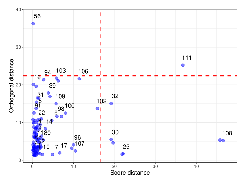
(a) Classical PCA

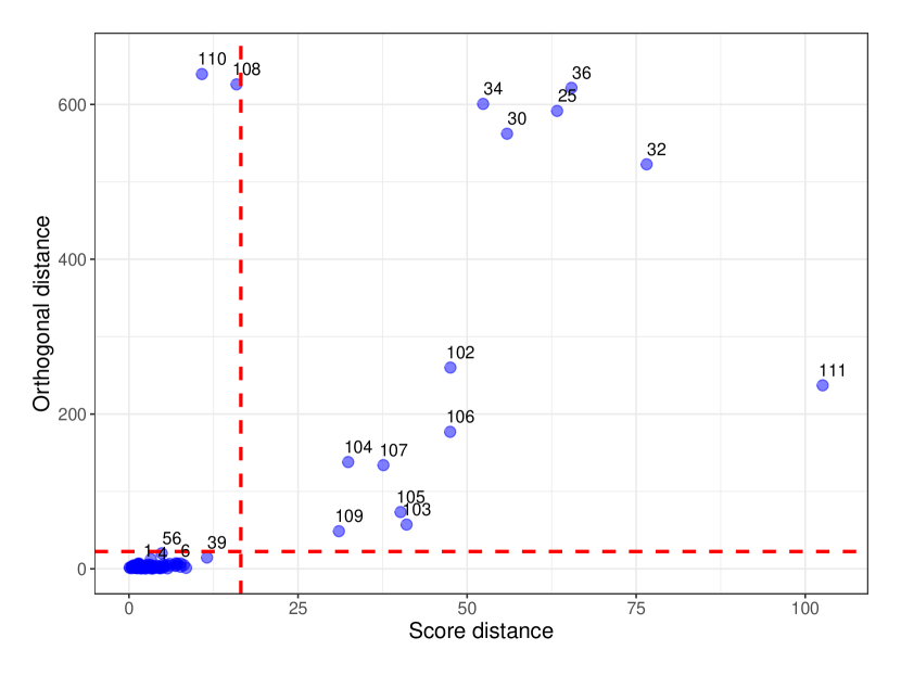
(b) rPCAdpd

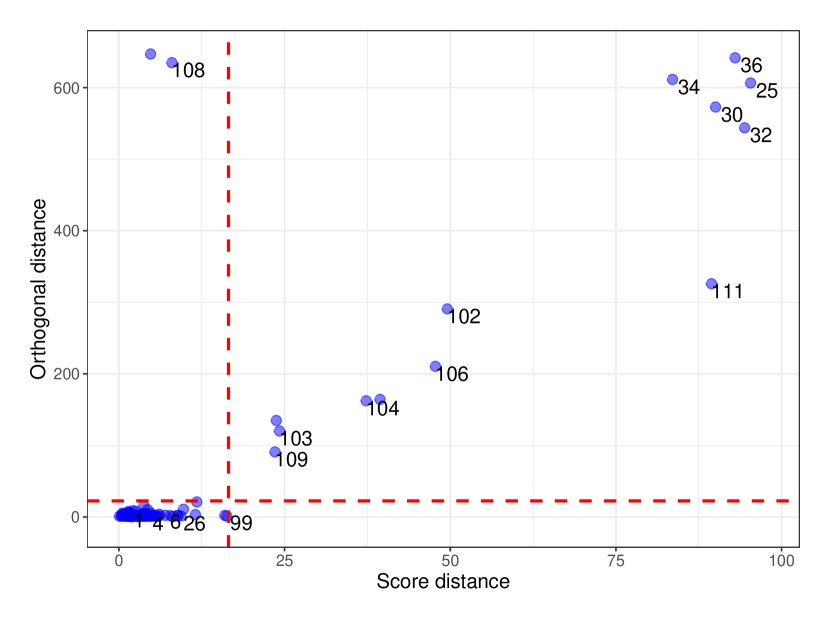
(c) ROBPCA

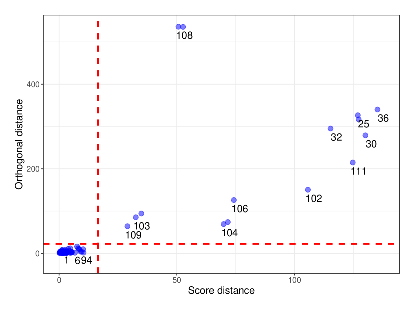
(d) Gmedian

Figure 1: Diagnostic plots for the Car dataset

5.2 Octane Data

The Octane dataset, sourced from Esbensen et al. [2002], features spectroscopic data with octane numbers derived from near-infrared (NIR) absorbance spectra of $39$ gasoline samples. Measurements span $226$ electromagnetic radiation wavelengths ($1102$ nm to $1552$ nm), each of which gives rise to a feature. With $39$ observations and $226$ features, principal component analysis (PCA) is pivotal for dimension reduction and subsequent analysis. Six samples ($25$, $26$, and $36-39$) contain additional alcohol, making them distinct [Hubert et al., 2005].

Similar to the Car dataset, a screenplot analysis reveals that there are only $2$ significant principal components present in the Octane dataset. However, the first principal value estimated by the classical PCA ($0.132$) is several magnitudes higher than the first principal value estimated by rPCAdpd ($0.01075$), which aligns with the estimates obtained from existing robust PCA algorithms [Hubert et al., 2005]. Diagnostic plots in Figure 2 demonstrate classical PCA’s failure to detect outliers, except observation $26$, while rPCAdpd identifies alcohol-mixed gasoline samples accurately. The ROBPCA algorithm also detects these outliers, with a similar score and orthogonal distances. However, the Gmedian algorithm labels most of these points as orthogonal outliers only.

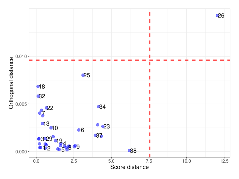
(a) Classical PCA

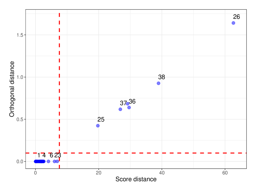
(b) rPCAdpd

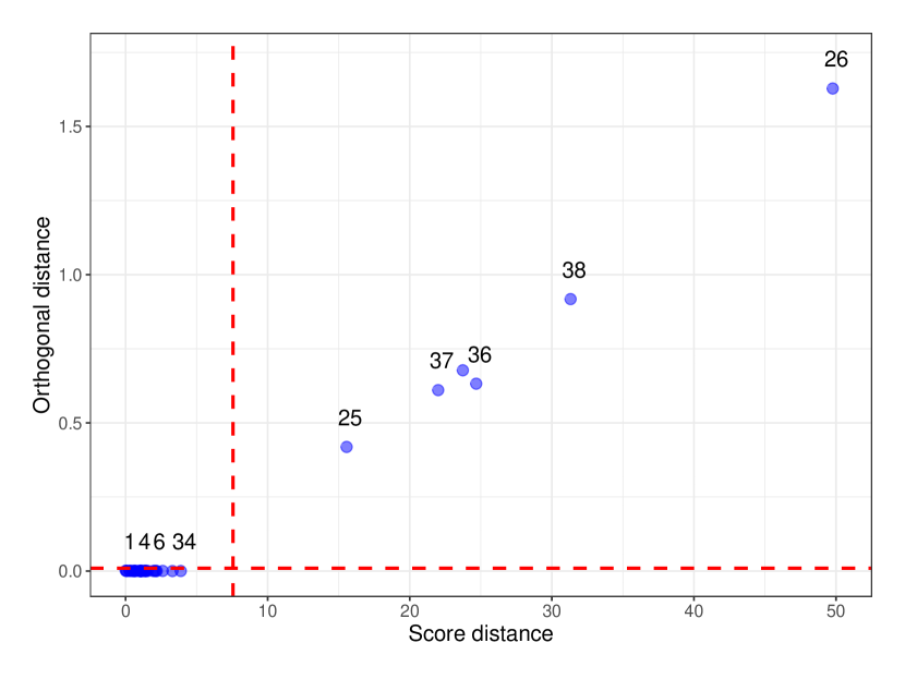
(c) ROBPCA

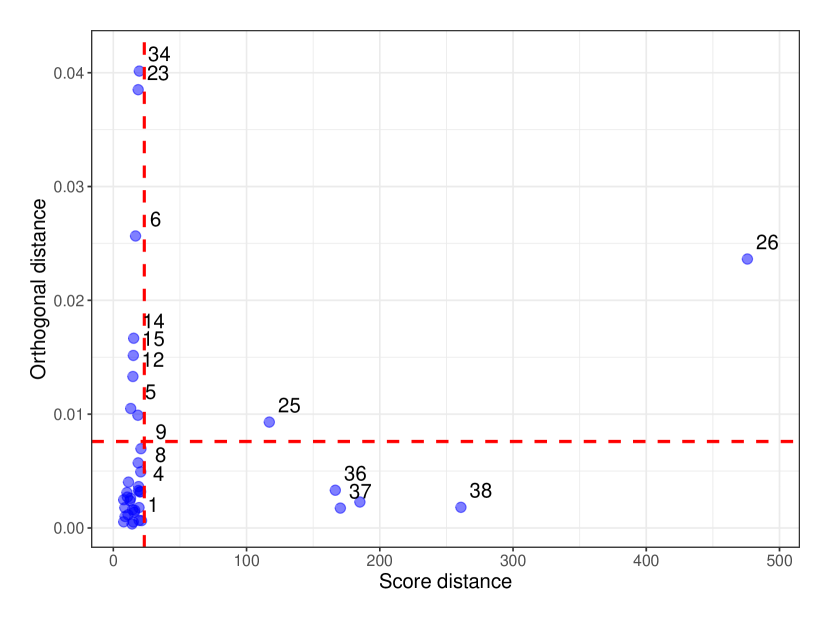
(d) GMedian

Figure 2: Diagnostic plots for the Octane dataset

5.3 Credit Card Fraud Detection

Credit card fraud detection is a very challenging problem because of the specific nature of transaction data and the labelling process. Most of the practical transaction data is highly imbalanced, and the number of fraudulent transactions is far too less compared to the extremely large number of valid transactions made on a day-to-day basis. There are primarily two kinds of strategies to detect such fraudulent transactions: the first one models the situation as a binary classification problem with some sampling procedures to counter class imbalance, and the second approach assumes that the fraudulent transactions are outliers in the data and applies an outlier detection algorithm. Many existing supervised and unsupervised machine learning algorithms [Carcillo et al., 2018, 2019] employ outlier detection to spot such fraudulent transactions. These methods often begin with a principal component analysis (PCA) to reduce dimensions and training time for real-time application.

To this end, we anticipate that the proposed robust PCA algorithm will outperform classical PCA in dimensionality reduction and provide reliable principal component estimates. We demonstrate this using the Credit Card Fraud Detection Dataset from Le Borgne and Bontempi [2004]. The dataset encompasses $28$ anonymized features over $284807$ transactions, with only $0.1\%$ ($492$) being fraudulent. For demonstration, we randomly sample $5\%$ of the dataset, including $19$ fraudulent transactions. The first $5$ principal components, explaining over $80\%$ of variation, are retained for both classical and rPCAdpd algorithms. Diagnostic plots in Figure 3 portray the outcomes, with red squares denoting fraudulent transactions. As shown in Figure 3, the classical PCA method fails to separate most of the fraudulent transactions, correctly identifying only $5$ (in red). In contrast, the rPCAdpd algorithm separates out $13$ out of $19$ outliers. Existing robust PCA methods such as ROBPCA and GMedian spot $7$ and $6$ outliers respectively, which are better than classical PCA but at the cost of many false positives (outliers without red squares). Thus, substituting classical PCA with the robust rPCAdpd algorithm in the preprocessing or dimensionality reduction step of this analysis can greatly enhance the results of the existing machine learning algorithms. By doing so, valuable insights about fraudulent transactions can assist the existing outlier detection and classification algorithms on the transformed, lower-dimensional data.

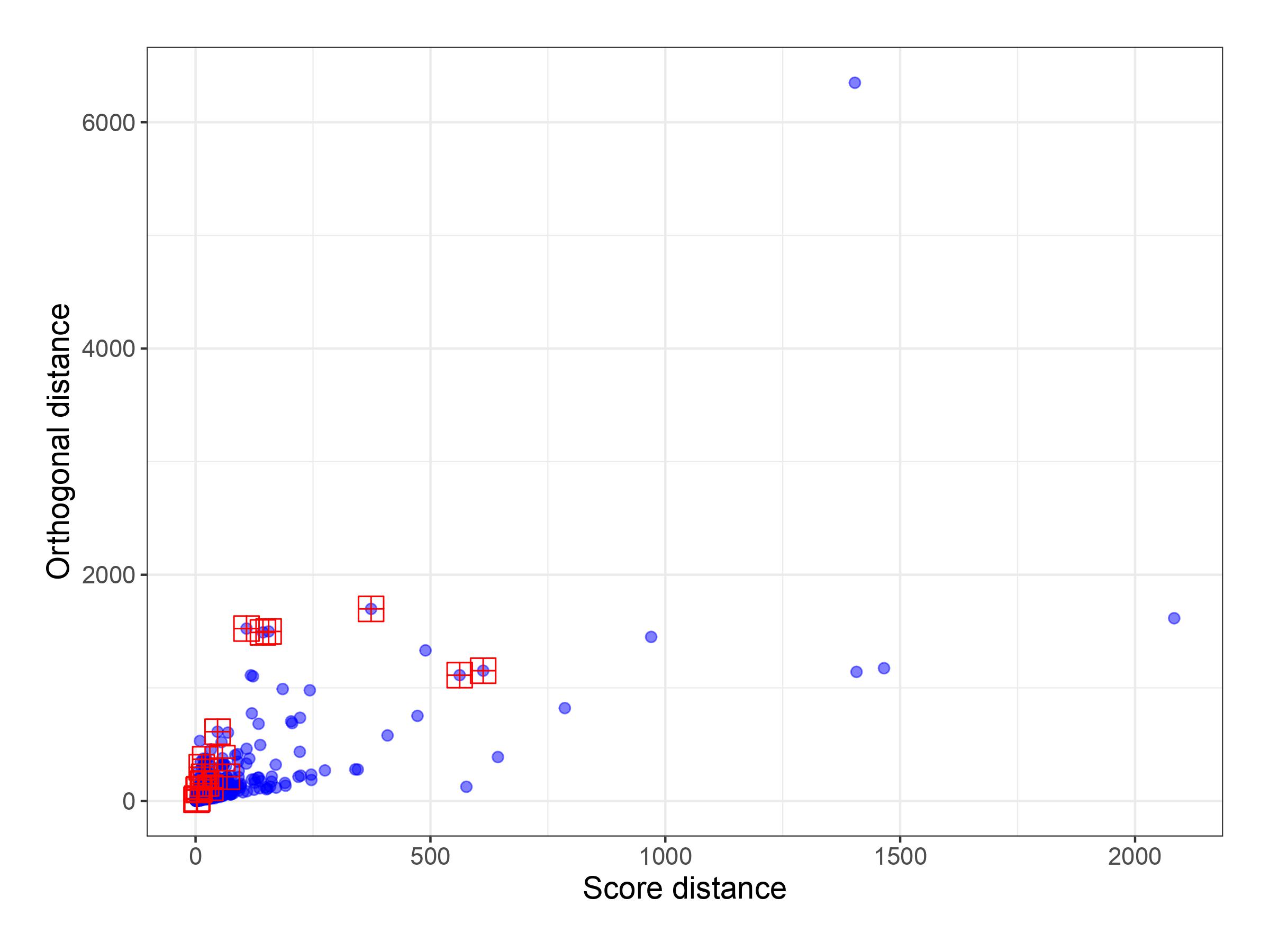
(a) Classical PCA

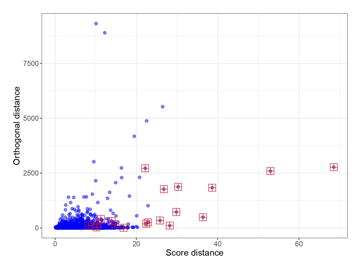
(b) rPCAdpd

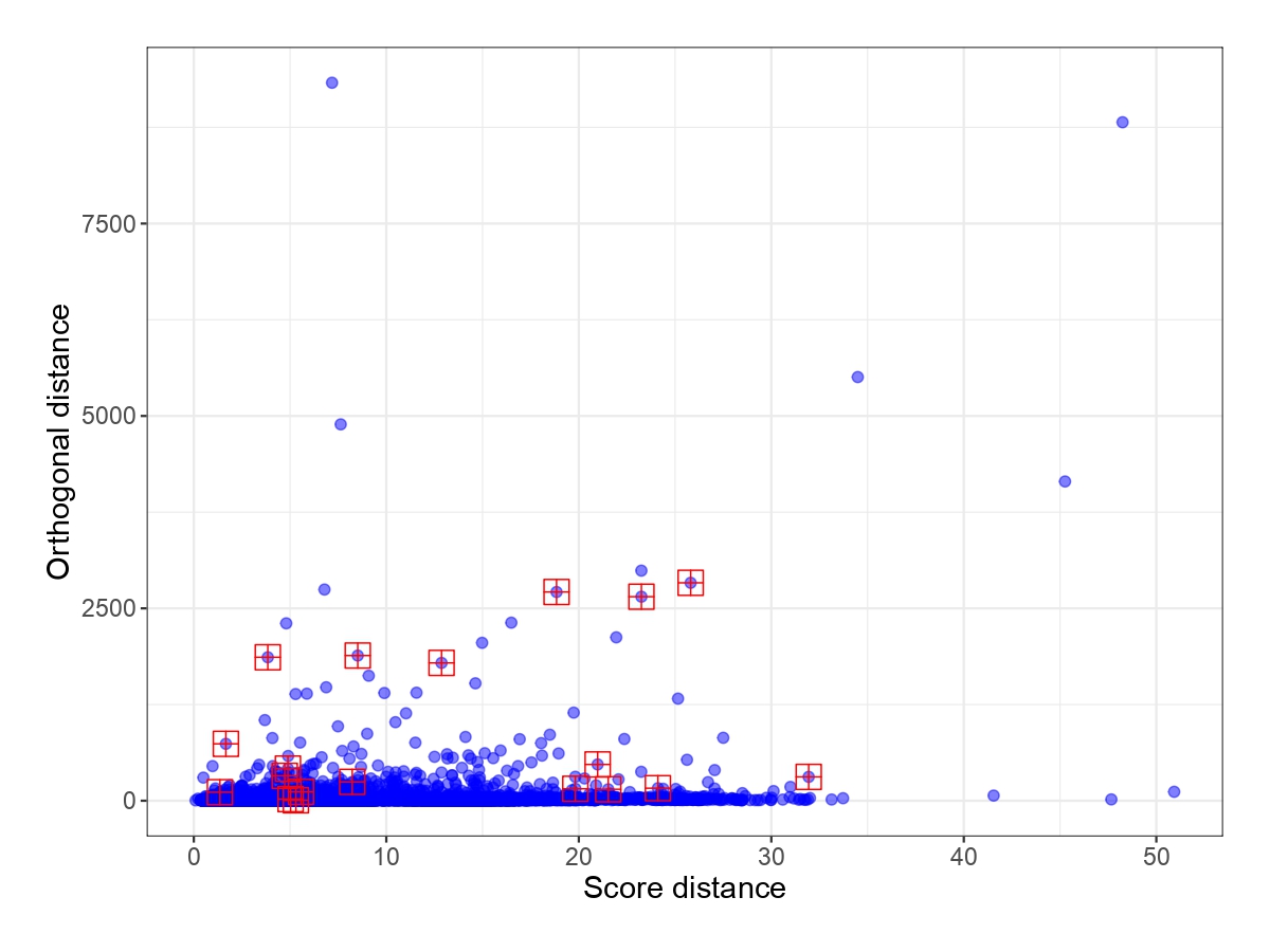
(c) ROBPCA

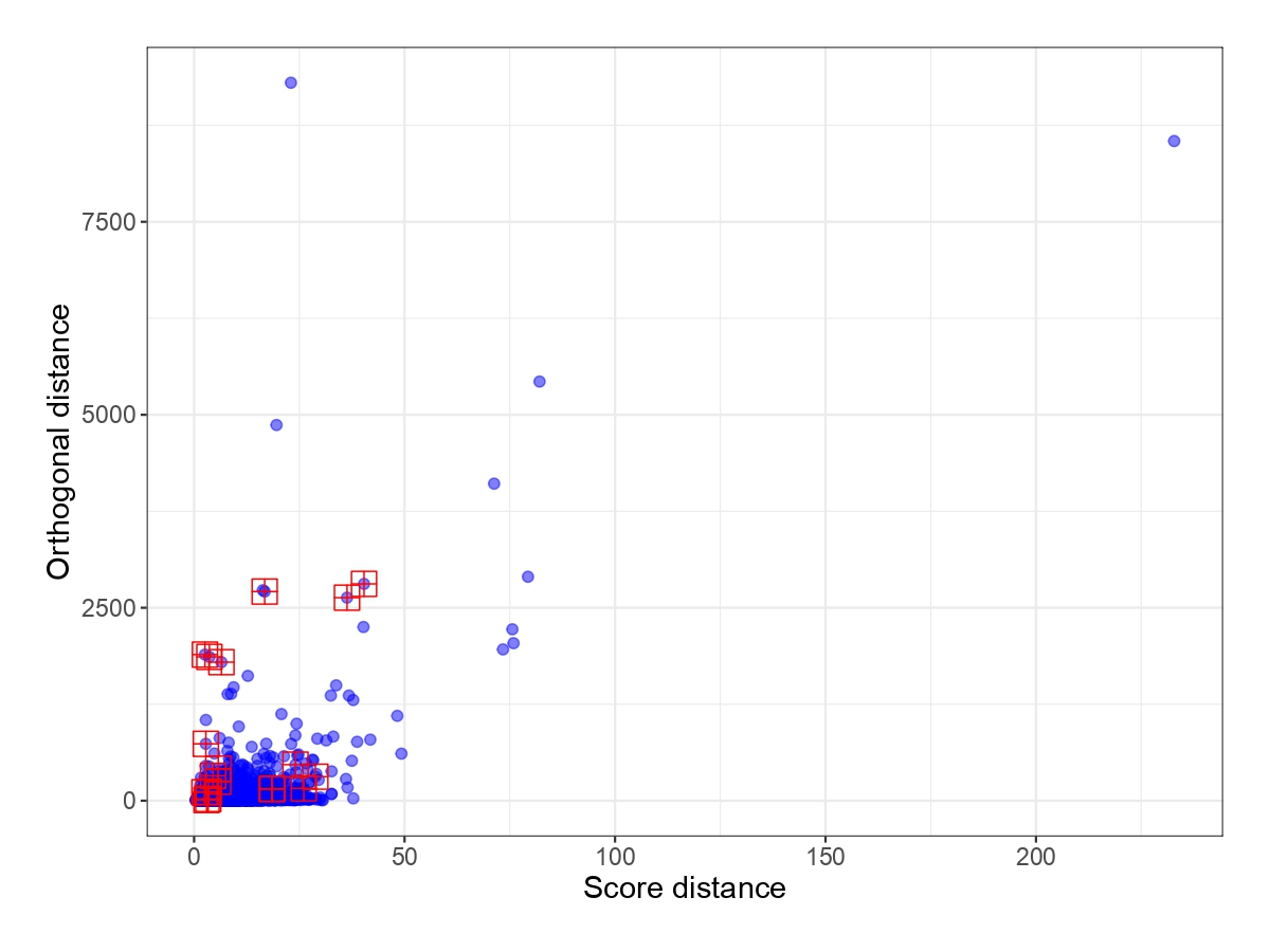
(d) GMedian

Figure 3: Diagnostic plots for the Credit Card dataset for different robust PCA methods

6 Conclusion

As described in Section 1, a plethora of algorithms from an extensive range of disciplines use principal component analysis. Unfortunately, with the emergence of the era of big data, it has become increasingly difficult to check or validate the authenticity, trustworthiness and overall correctness of the data. As a result, most of the input data to these algorithms are highly susceptible of being contaminated by various forms of noise and outlying observations. Since classical PCA is heavily affected by such outliers, several robust PCA algorithms have been proposed in the last two decades. Many of these are not both fast and scalable. M-estimation based techniques are computationally efficient to obtain, but their breakdown point decays rapidly with the increase in dimension making it unacceptable for being used for high dimensional data. On the other hand, MVE, MCD and other projection pursuit based methods are highly scalable, but they are either computationally extremely intensive or lack proper theoretical guarantees of consistency, asymptotic normality or bounded influence function along with high breakdown. We believe that this paper will help to fill this gap by providing a robust, scalable and efficient PCA estimator with the help of the popular density power divergence. We demonstrate its various desirable theoretical properties in the present work. It also has a dimension-free breakdown point making it attractive to be used in arbitrarily high dimensional data analysis. Also, the robustness parameter $\alpha$ in rPCAdpd can be tuned to provide a smooth bridge between efficiency in estimation and robustness capabilities.

In all the datasets used to describe the practical applicability of the rPCAdpd, we estimate the significant number of principal components to be extracted based on thresholding the proportion of the variation explained by the first few principal components. However, such a procedure would require the estimation of all principal components first and then computing the proportion. From a computational point of view, it is highly beneficial to estimate the rank of the low-rank matrix $\boldsymbol{L}$ first, and then proceed with the estimation of principal components. We will investigate this direction in a future study.

Appendix A Proofs of the Results

A.1 Normalization constant of Elliptically Symmetric Families of Distributions

Here we show that the normalizing constant for the elliptically symmetric family of densities is of the form $c_{g}\det(\boldsymbol{\Sigma})^{1/2}$. To see this, we note that it can be expressed as

$$\mathcal{C}_{g}=\int_{\mathbb{R}^{p}}\exp\left[g\left((\boldsymbol{x}-\boldsymbol{\mu})^{\intercal}\sum_{k=1}^{p}\gamma_{k}^{-1}\boldsymbol{v}_{k}\boldsymbol{v}_{k}^{\intercal}(\boldsymbol{x}-\boldsymbol{\mu})\right)\right]d\boldsymbol{x}.$$

Let $\boldsymbol{P}$ be the $p\times p$ orthogonal matrix whose rows are the vectors $\boldsymbol{v}_{k}^{\intercal}$ for $k=1,2,\dots p$. Then, applying a change of variable $\boldsymbol{z}=\boldsymbol{P}^{\intercal}(\boldsymbol{x}-\boldsymbol{\mu})$, we can rewrite the integral as

$$\mathcal{C}_{g}=\int_{\mathbb{R}^{p}}\exp\left[g\left(\sum_{k=1}^{p}\gamma_{k}^{-1}z_{k}^{2}\right)\right]d\boldsymbol{z},$$

where $\boldsymbol{z}=(z_{1},z_{2},\dots z_{p})^{\intercal}$. Finally, another change of variable with $u_{k}=z_{k}/\sqrt{\gamma_{k}}$ for $k=1,2,\dots p$ yields,

$$\mathcal{C}_{g}=\int_{\mathbb{R}^{p}}2^{-p}\prod_{k=1}^{p}\gamma_{k}^{1/2}\prod_{k=1}^{p}u_{k}^{-1/2}\exp\left[g\left(\sum_{k=1}^{p}u_{k}^{2}\right)\right]du_{1}du_{2}\dots du_{p}=\det(\boldsymbol{\Sigma})^{1/2}c_{g},$$

where the constant $c_{g}$ is the integral it is replacing. Clearly, the term $c_{g}$ is free of the mean $\boldsymbol{\mu}$ and the dispersion $\boldsymbol{\Sigma}$ matrix, and hence is a constant depending only on the $g$ function.

A.2 Proof of Theorem 3.1

First note that the eigenvectors $\boldsymbol{v}_{k}$ lie in the Stiefel manifold of order $p$, which is a closed and bounded subset of $\mathbb{R}^{p}$, hence is compact.

Also, since $g(x)$ is a continuous decreasing function, $\lim_{x\rightarrow\infty}e^{g(x)}=0$. Otherwise if $\lim_{x\rightarrow\infty}e^{g(x)}=\epsilon>0$, it implies that the integral $\int_{0}^{\infty}e^{g(x)}$ diverges by comparison test, contradicting the existence of the elliptically symmetric probability density function.

Fixing $\boldsymbol{\mu}\in\mathbb{R}^{p}$, let us now observe how the objective function $Q$ behaves for extreme values of the eigenvalues $\gamma_{1},\dots\gamma_{p}$. If $\gamma_{1}\rightarrow 0$, then it follows that

$$\lim_{\gamma_{1}\rightarrow 0}Q(\gamma_{1},\dots,\gamma_{p},\boldsymbol{\eta})=\lim_{\gamma_{1}\rightarrow 0}\gamma_{1}^{-1/2}\left[\dfrac{c_{(1+\alpha)g}}{c_{g}}-\lim_{x\rightarrow\infty}e^{g(x)}\right]\geq 0,$$

since $c_{g}>0$ for any choice of $g$ function by definition. On the other hand, if $\gamma_{1}\rightarrow\infty$, the quadratic form

$$(\boldsymbol{X}_{i}-\boldsymbol{\mu})^{\intercal}\sum_{k=1}^{p}\gamma_{k}^{-1}\boldsymbol{v}_{k}(\boldsymbol{\eta})\boldsymbol{v}_{k}(\boldsymbol{\eta})^{\intercal}(\boldsymbol{X}_{i}-\boldsymbol{\mu})\rightarrow(\boldsymbol{X}_{i}-\boldsymbol{\mu})^{\intercal}\sum_{k=2}^{p}\gamma_{k}^{-1}\boldsymbol{v}_{k}(\boldsymbol{\eta})\boldsymbol{v}_{k}(\boldsymbol{\eta})^{\intercal}(\boldsymbol{X}_{i}-\boldsymbol{\mu}).$$

Then by the strong law of large numbers, it follows that for sufficiently large $n$, with probability $1$,

$$\dfrac{1}{n}\sum_{i=1}^{n}\exp\left\{\alpha g\left((\boldsymbol{X}_{i}-\boldsymbol{\mu})^{\intercal}\sum_{k=2}^{p}\gamma_{k}^{-1}\boldsymbol{v}_{k}(\boldsymbol{\eta})\boldsymbol{v}_{k}(\boldsymbol{\eta})^{\intercal}(\boldsymbol{X}_{i}-\boldsymbol{\mu})\right)\right\}$$

$$\rightarrow\quad \mathbb{E}\left[\exp\left\{\alpha g\left((\boldsymbol{X}-\boldsymbol{\mu})^{\intercal}\sum_{k=2}^{p}\gamma_{k}^{-1}\boldsymbol{v}_{k}(\boldsymbol{\eta})\boldsymbol{v}_{k}(\boldsymbol{\eta})^{\intercal}(\boldsymbol{X}-\boldsymbol{\mu})\right)\right\}\right]$$

$$\geq\quad \mathbb{E}\left[\exp\left\{\alpha g\left((\boldsymbol{X}-\boldsymbol{\mu})^{\intercal}\sum_{k=1}^{p}\gamma_{k}^{-1}\boldsymbol{v}_{k}(\boldsymbol{\eta})\boldsymbol{v}_{k}(\boldsymbol{\eta})^{\intercal}(\boldsymbol{X}-\boldsymbol{\mu})\right)\right\}\right]$$

$$=\quad \int_{R^{p}}\exp\left\{(1+\alpha)g\left((\boldsymbol{x}-\boldsymbol{\mu})^{\intercal}\sum_{k=1}^{p}\gamma_{k}^{-1}\boldsymbol{v}_{k}(\boldsymbol{\eta})\boldsymbol{v}_{k}(\boldsymbol{\eta})^{\intercal}(\boldsymbol{x}-\boldsymbol{\mu})\right)\right\}d\boldsymbol{x}$$

$$=\quad \dfrac{c_{(1+\alpha)g}}{c_{g}},$$

where the inequality uses the fact that $g$ is monotonically decreasing. Therefore, for sufficiently large $n$, with probability $1$, $Q(\gamma_{1},\dots\gamma_{p},\boldsymbol{\eta})$ increases to $0$ as $\gamma_{1}$ increases to $\infty$. Therefore, for any given $\epsilon>0$, there exists $0<a_{1}<b_{1}<\infty$ such that $Q(\gamma_{1},\gamma_{2},\dots\gamma_{p})>(-\epsilon)$ for any $\gamma_{1}\not\in[a_{1},b_{1}]$. Note that, since $\gamma_{1}$ is chosen arbitrarily, the same conclusion also holds for all other eigenvalues, possibly with different choices of $a_{k}$ and $b_{k}$ for $k=1,2,\dots p$. Letting, $\epsilon=-\inf Q(\gamma_{1},\dots\gamma_{p},\boldsymbol{\eta})/2$ (which is finite by continuity of $Q$ and the limiting behaviour described above) and considering the set $K=\prod_{k=1}^{p}[a_{k},b_{k}]\times S$, we note that the infimum of $Q$ must exist within the set $K$. Since $K$ is a compact subset of $\mathbb{R}^{p}$, it follows by the Extreme Value Theorem that the infimum must be attained. This proves the existence of the rPCAdpd estimator for any arbitrary value of $\mu$, including the location estimate $\widehat{\mu}$.

A.3 Proof of Theorem 3.2

Let $\widehat{\boldsymbol{\mu}}_{Y}$ and $\widehat{\boldsymbol{\mu}}_{X}$ be the robust estimates of the location based on the sample $\boldsymbol{Y}_{1},\dots\boldsymbol{Y}_{n}$ and $\boldsymbol{X}_{1},\dots\boldsymbol{X}_{n}$ respectively. Then by the orthogonal equivariance of the location estimator, we have that $\widehat{\boldsymbol{\mu}}_{Y}=a\boldsymbol{P}\widehat{\boldsymbol{\mu}}_{X}+\boldsymbol{b}$. The equivariance property for the estimated eigenvalues and eigenvectors by the rPCAdpd algorithm then follows from the observation that the quadratic form of the transformed data can be expressed as

$$(\boldsymbol{Y}_{i}-\widehat{\boldsymbol{\mu}}_{Y})^{\intercal}\left(\sum_{k=1}^{p}\gamma_{k}^{-1}\boldsymbol{v}_{k}\boldsymbol{v}_{k}^{\intercal}\right)(\boldsymbol{Y}_{i}-\widehat{\boldsymbol{\mu}}_{Y}) =a(\boldsymbol{X}_{i}-\widehat{\boldsymbol{\mu}}_{X})^{\intercal}\boldsymbol{P}^{\intercal}\left(\sum_{k=1}^{p}\gamma_{k}^{-1}\boldsymbol{v}_{k}\boldsymbol{v}_{k}^{\intercal}\right)(\boldsymbol{X}_{i}-\widehat{\boldsymbol{\mu}}_{X})\boldsymbol{P}a$$

$$=(\boldsymbol{X}_{i}-\widehat{\boldsymbol{\mu}}_{X})^{\intercal}\left(\sum_{k=1}^{p}(\gamma_{k}/a^{2})^{-1}\boldsymbol{P}^{\intercal}\boldsymbol{v}_{k}\boldsymbol{v}_{k}^{\intercal}\boldsymbol{P}\right)(\boldsymbol{X}_{i}-\widehat{\boldsymbol{\mu}}_{X}).$$

It shows that, if rPCAdpd estimates of the eigenvalues for the sample $\boldsymbol{X}_{1},\dots\boldsymbol{X}_{p}$ are $\gamma_{k}^{\ast}$ for $k=1,2,\dots p$ respectively, then the rPCAdpd estimate of the same for the transformed sample would be $a^{2}\gamma_{k}^{\ast}$. A similar conclusion can be drawn for the rPCAdpd estimate of eigenvectors as well.

A.4 Proof of Lemma 3.1

Let, $h_{\boldsymbol{\theta}}(\boldsymbol{x})=c^{-1}_{\alpha}(\boldsymbol{\theta})f^{(1+\alpha)}_{\boldsymbol{\theta}}(\boldsymbol{x})$ be another density function. Note that

$$\dfrac{\partial}{\partial\boldsymbol{\theta}}\log(h_{\boldsymbol{\theta}}(\boldsymbol{x}))=-\dfrac{\partial}{\partial\boldsymbol{\theta}}\log(c_{\alpha}(\boldsymbol{\theta}))+(1+\alpha)u_{\boldsymbol{\theta}}(\boldsymbol{x}),$$

where $u_{\theta}(\boldsymbol{x})$ is the score function corresponding to $f_{\boldsymbol{\theta}}(\boldsymbol{x})$. Under the standard regularity conditions, one can exchange the differentiation and the integral sign to obtain that the expectation of the score function is equal to $0$. Therefore,

$$0=\int\dfrac{\partial}{\partial\boldsymbol{\theta}}\log(h_{\boldsymbol{\theta}}(\boldsymbol{x}))h_{\boldsymbol{\theta}}(\boldsymbol{x})d\boldsymbol{x}=-\dfrac{\partial}{\partial\boldsymbol{\theta}}\log(c_{\alpha}(\boldsymbol{\theta}))+\dfrac{(1+\alpha)}{c_{\alpha}(\boldsymbol{\theta})}\xi_{\boldsymbol{\theta}}.$$

Interchanging the sides and solving for $\xi_{\boldsymbol{\theta}}$ yields the result.

A.5 Proof of Lemma 3.2

Starting with the decomposition

$$u^{h}_{\boldsymbol{\theta}}(\boldsymbol{x})=\dfrac{\partial}{\partial\boldsymbol{\theta}}\log(h_{\boldsymbol{\theta}}(\boldsymbol{x}))=-\dfrac{\partial}{\partial\boldsymbol{\theta}}\log(c_{\alpha}(\boldsymbol{\theta}))+(1+\alpha)u_{\boldsymbol{\theta}}(\boldsymbol{x}),$$

it follows that

$$\begin{split}\left(u^{h}_{\boldsymbol{\theta}}(\boldsymbol{x})\right)\left(u^{h}_{\boldsymbol{\theta}}(\boldsymbol{x})\right)^{\intercal}&=\left(\dfrac{\partial}{\partial\boldsymbol{\theta}}\log(c_{\alpha}(\boldsymbol{\theta}))\right)\left(\dfrac{\partial}{\partial\boldsymbol{\theta}}\log(c_{\alpha}(\boldsymbol{\theta}))\right)^{\intercal}\\ &+2(1+\alpha)u_{\boldsymbol{\theta}}(\boldsymbol{x})\left(\dfrac{\partial}{\partial\boldsymbol{\theta}}\log(c_{\alpha}(\boldsymbol{\theta}))\right)^{\intercal}+(1+\alpha)^{2}u_{\boldsymbol{\theta}}(\boldsymbol{x})u^{\intercal}_{\boldsymbol{\theta}}(\boldsymbol{x}).\end{split}$$

Multiplying both sides with $h_{\boldsymbol{\theta}}(\boldsymbol{x})$ and integrating with respect to $\boldsymbol{x}$ yields

$$i^{h}(\boldsymbol{\theta})=\left(\dfrac{\nabla_{\boldsymbol{\theta}}c_{\alpha}(\boldsymbol{\theta})}{c_{\alpha}(\boldsymbol{\theta})}\right)\left(\dfrac{\nabla_{\boldsymbol{\theta}}c_{\alpha}(\boldsymbol{\theta})}{c_{\alpha}(\boldsymbol{\theta})}\right)^{\intercal}-2\left(\dfrac{\nabla_{\boldsymbol{\theta}}c_{\alpha}(\boldsymbol{\theta})}{c_{\alpha}(\boldsymbol{\theta})}\right)\left(\dfrac{\nabla_{\boldsymbol{\theta}}c_{\alpha}(\boldsymbol{\theta})}{c_{\alpha}(\boldsymbol{\theta})}\right)^{\intercal}+\dfrac{(1+\alpha)^{2}}{c_{\alpha}(\boldsymbol{\theta})}J_{\boldsymbol{\theta}},$$

where $\nabla_{\boldsymbol{\theta}}c_{\alpha}(\boldsymbol{\theta})=\frac{\partial c_{\alpha}(\boldsymbol{\theta})}{\partial\boldsymbol{\theta}}$. Solving for $J_{\boldsymbol{\theta}}$ yields Eq. (3.4).

A.6 Proof of Corollary 3.2

Since the normalized density $c_{\alpha}^{-1}(\boldsymbol{\theta})f_{\boldsymbol{\theta}}^{(1+\alpha)}$ also belongs to an elliptically symmetric class of densities, it follows that

$$c_{\alpha}(\boldsymbol{\theta})=c_{(1+\alpha)g}\prod_{k=1}^{p}(\gamma_{k})^{1/2}c_{g}^{-(1+\alpha)}\prod_{k=1}^{p}(\gamma_{k})^{-(1+\alpha)/2}.$$

Putting this value and its derivative with respect to $\boldsymbol{\theta}$ into Lemma 3.1 yields Corollary 3.2.

A.7 Proof of Corollary 3.3

We start by defining a few notations as follows:

$$Q(\boldsymbol{x}) =(\boldsymbol{x}-\boldsymbol{\mu}^{\ast})^{\intercal}\left(\sum_{k=1}^{p}\gamma_{k}^{-1}\boldsymbol{v}_{k}\boldsymbol{v}_{k}^{\intercal}\right)(\boldsymbol{x}-\boldsymbol{\mu}^{\ast}),$$

$$A_{2}(g) =\int g^{\prime}(Q(\boldsymbol{x}))(\boldsymbol{x}-\boldsymbol{\mu}^{\ast})(\boldsymbol{x}-\boldsymbol{\mu}^{\ast})^{\intercal}c_{0}(\boldsymbol{\theta})^{-1}\exp(g(Q(\boldsymbol{x})))d\boldsymbol{x},$$

$$A_{4}(g;\boldsymbol{u},\boldsymbol{v}) =\int\left(g^{\prime}(Q(\boldsymbol{x}))\right)^{2}(\boldsymbol{x}-\boldsymbol{\mu}^{\ast})(\boldsymbol{x}-\boldsymbol{\mu}^{\ast})^{\intercal}\boldsymbol{u}\boldsymbol{v}^{\intercal}(\boldsymbol{x}-\boldsymbol{\mu}^{\ast})(\boldsymbol{x}-\boldsymbol{\mu}^{\ast})^{\intercal}c_{0}(\boldsymbol{\theta})^{-1}\exp(g(Q(\boldsymbol{x})))d\boldsymbol{x}.$$

Here, $c_{0}(\boldsymbol{\theta})$ is the normalizing constant the normalizing constant for the elliptically symmetric density proportional to $\exp(g(Q(\boldsymbol{x}))$. Clearly, $c_{0}(\boldsymbol{\theta})=c_{g}\prod_{k=1}^{p}\gamma_{k}^{1/2}$. All of these quantities are well defined due to the Assumptions (A1) and (A3). Also, let $\boldsymbol{G}_{k}=\frac{\partial\boldsymbol{v}_{k}}{\partial\boldsymbol{\eta}}$ denote the $p(p+1)/2\times p$ matrix whose columns are the gradients of the entries $v_{kj}$ for $j=1,2,\dots p$, of $\boldsymbol{v}_{k}$ with respect to the parameter $\boldsymbol{\eta}$. One important aspect is to note the quantities $A_{2}(g)$ and $A_{4}(g;\boldsymbol{u},\boldsymbol{v})$ are free of $\boldsymbol{\mu}^{\ast}$, which can be verified by a simple substitution in the integral.

Starting with the identity

$$c_{0}(\boldsymbol{\theta})=\int\exp\left(g(Q(\boldsymbol{x}))\right)d\boldsymbol{x},$$

and differentiating both sides by $\gamma_{k}$ and $\boldsymbol{\eta}$ respectively, we obtain the identities

$$\gamma_{k}^{-2}\boldsymbol{v}_{k}^{\intercal}A_{2}(g)\boldsymbol{v}_{k}=-\dfrac{1}{2\gamma_{k}},\ \sum_{k=1}^{p}\gamma_{k}^{-1}\boldsymbol{G}_{k}A_{2}(g)\boldsymbol{v}_{k}=0,$$ (A.1)

both of which will be used later in the proof.

Let $h_{\boldsymbol{\theta}}(\boldsymbol{x})=c_{(1+\alpha)}(\boldsymbol{\theta})^{-1}e^{(1+\alpha)g(Q(\boldsymbol{x}))}$ be a density belonging to the same elliptically symmetric family. Then, the score function $u_{\boldsymbol{\theta}}^{h}(\boldsymbol{x})$ corresponding to $h_{\boldsymbol{\theta}}$ can be expressed as

$$u_{\boldsymbol{\theta}}^{h}(\boldsymbol{x})=\begin{bmatrix}\frac{1}{2}\text{Diag}\left(\boldsymbol{\Gamma}^{-1}\right)-(1+\alpha)g^{\prime}(Q(\boldsymbol{x}))\boldsymbol{\Gamma}^{-2}\boldsymbol{V}^{\intercal}(\boldsymbol{I}_{p}\otimes(\boldsymbol{x}-\boldsymbol{\mu})(\boldsymbol{x}-\boldsymbol{\mu})^{\intercal})\boldsymbol{V}\\ 2(1+\alpha)g^{\prime}(Q(\boldsymbol{x}))\boldsymbol{G}(\boldsymbol{\Gamma}^{-1}\otimes(\boldsymbol{x}-\boldsymbol{\mu})(\boldsymbol{x}-\boldsymbol{\mu})^{\intercal})\boldsymbol{V}\boldsymbol{1}_{p}\end{bmatrix}.$$ (A.2)

Using the expression for $u_{\boldsymbol{\theta}}^{h}(\boldsymbol{x})$, we can further differentiate this with respect to the entries of $\boldsymbol{\theta}$ and take expectation. This leads to the Fisher Information matrix in the partitioned form as follows,

$$i^{h}(\boldsymbol{\theta})=\begin{bmatrix}i^{h}(\gamma_{1},\gamma_{1})&\dots&i^{h}(\gamma_{1},\gamma_{p})&i^{h}(\gamma_{1},\boldsymbol{\eta})\\ \vdots&\ddots&\vdots&\vdots\\ i^{h}(\gamma_{p},\gamma_{1})&\dots&i^{h}(\gamma_{p},\gamma_{p})&i^{h}(\gamma_{p},\boldsymbol{\eta})\\ i^{h}(\gamma_{1},\boldsymbol{\eta})^{\intercal}&\dots&i^{h}(\gamma_{p},\boldsymbol{\eta})^{\intercal}&i^{h}(\boldsymbol{\eta},\boldsymbol{\eta})\end{bmatrix},$$

where,

$$i^{h}(\gamma_{k},\gamma_{l}) =\left(\dfrac{\partial q_{(1+\alpha)g}}{\partial\gamma_{k}}\right)\left(\dfrac{\partial q_{(1+\alpha)g}}{\partial\gamma_{l}}\right)+\left(\dfrac{\partial q_{(1+\alpha)g}}{\partial\gamma_{k}}\right)\gamma_{l}^{-2}\boldsymbol{v}_{l}^{\intercal}A_{2}((1+\alpha)g)\boldsymbol{v}_{l}$$

$$\qquad+\left(\dfrac{\partial q_{(1+\alpha)g}}{\partial\gamma_{l}}\right)\gamma_{k}^{-2}\boldsymbol{v}_{k}^{\intercal}A_{2}((1+\alpha)g)\boldsymbol{v}_{k}+\dfrac{\boldsymbol{v}_{k}^{\intercal}A_{4}((1+\alpha)g;\boldsymbol{v}_{k},\boldsymbol{v}_{l})\boldsymbol{v}_{l}}{\gamma_{k}^{2}\gamma_{l}^{2}}$$

$$=-\left(\dfrac{\partial q_{(1+\alpha)g}}{\partial\gamma_{k}}\right)\left(\dfrac{\partial q_{(1+\alpha)g}}{\partial\gamma_{l}}\right)+\dfrac{\boldsymbol{v}_{k}^{\intercal}A_{4}((1+\alpha)g;\boldsymbol{v}_{k},\boldsymbol{v}_{l})\boldsymbol{v}_{l}}{\gamma_{k}^{2}\gamma_{l}^{2}},\ k,l=1,2,\dots p$$

$$i^{h}(\gamma_{k},\boldsymbol{\eta}) =-2\left(\dfrac{\partial q_{(1+\alpha)g}}{\partial\gamma_{k}}\right)\sum_{k=1}^{p}\gamma_{k}^{-1}\boldsymbol{G}_{k}A_{2}((1+\alpha)g)\boldsymbol{v}_{k}-\dfrac{2}{\gamma_{k}^{2}}\sum_{l=1}^{p}\gamma_{l}^{-1}\boldsymbol{v}_{k}^{\intercal}A_{4}((1+\alpha)g;\boldsymbol{v}_{k},\boldsymbol{v}_{l})\boldsymbol{G}_{l}^{\intercal}$$

$$=-\dfrac{2}{\gamma_{k}^{2}}\sum_{l=1}^{p}\gamma_{l}^{-1}\boldsymbol{v}_{k}^{\intercal}A_{4}((1+\alpha)g;\boldsymbol{v}_{k},\boldsymbol{v}_{l})G_{l}^{\intercal},\ k=1,\dots p$$

$$i^{h}(\boldsymbol{\eta},\boldsymbol{\eta}) =4\sum_{k=1}^{p}\sum_{l=1}^{p}\gamma_{k}^{-1}\gamma_{l}^{-1}\boldsymbol{G}_{k}A_{4}((1+\alpha)g;\boldsymbol{v}_{k},\boldsymbol{v}_{l})\boldsymbol{G}_{l}^{\intercal},$$

where we use the identities (A.1). In all of the above expressions, the quantity $q_{g}$ denoted the logarithm of the normalizing constant, i.e., $q_{g}=\log(c_{0}(\boldsymbol{\theta}))$ and $q_{(1+\alpha)g}=\log(c_{\alpha}(\boldsymbol{\theta}))$. Finally, Corollary 3.3 follows from using Lemma 3.2 and the expression of $\boldsymbol{\xi}_{\boldsymbol{\theta}}$ given in Corollary 3.2.

A.8 Proof of the Theorem 3.4

The proof of the Theorem 3.4 closely resembles the proof of Theorem 3.1 of Ghosh and Basu [2013]. For brevity, we shall only indicate the modifications pertinent to the special scenario of principal components. Given the location estimator $\widehat{\boldsymbol{\mu}}$, using the same notation as in Ghosh and Basu [2013], we define

$$V(\boldsymbol{X},\boldsymbol{\theta})=\prod_{k=1}^{p}\gamma_{k}^{-\alpha/2}\left[\dfrac{c_{(1+\alpha)g}}{c_{g}}-\left(1+\dfrac{1}{\alpha}\right)e^{\alpha g\left((\boldsymbol{X}-\widehat{\boldsymbol{\mu}})^{\intercal}\sum_{k=1}^{p}\gamma_{k}^{-1}\boldsymbol{v}_{k}(\boldsymbol{\eta})\boldsymbol{v}_{k}(\boldsymbol{\eta})^{\intercal}(\boldsymbol{X}-\widehat{\boldsymbol{\mu}})\right)}\right]$$

which are the summands in the objective function in Eq. (3.1). Now, conditional on $\widehat{\boldsymbol{\mu}}$, by an application of the Law of Large Numbers, we have

$$\dfrac{1}{n}\sum_{i=1}^{n}\nabla V(\boldsymbol{X}_{i},\boldsymbol{\theta}^{\ast})\mid\widehat{\boldsymbol{\mu}}\xrightarrow{P}0,\ \text{and, }\ \dfrac{1}{n}\sum_{i=1}^{n}\nabla^{2}V(\boldsymbol{X}_{i},\boldsymbol{\theta}^{\ast})\mid\widehat{\boldsymbol{\mu}}\xrightarrow{P}\boldsymbol{J}_{\boldsymbol{\theta}^{\ast}}$$

where $\boldsymbol{\theta}^{\ast}$ is the true value of the parameters. Now, since the right-hand sides of both of these are continuous functions of $\widehat{\boldsymbol{\mu}}$ and as $\widehat{\boldsymbol{\mu}}\xrightarrow{P}\boldsymbol{\mu}^{\ast}$ (the true location parameter) due to the consistency of the location estimator, it follows that the unconditional random variables also converges in probability to the same value. As the support of the elliptically symmetric family of distributions is assumed to be the entire space $\mathbb{R}^{p}$, $\boldsymbol{J}_{\boldsymbol{\theta}^{\ast}}$ becomes free of the choice of location which makes this convergence possible. Now, one can replicate the proof for consistency to show that the rPCAdpd estimator is consistent.

To prove the asymptotic normality, we need to show that $T_{n}=\frac{1}{\sqrt{n}}\sum_{i=1}^{n}\nabla^{2}V(\boldsymbol{X}_{i},\boldsymbol{\theta}^{\ast})$ converges in distribution to a random variable $\boldsymbol{Z}$ following a multivariate normal distribution with mean $0$ and variance $\boldsymbol{K}_{\boldsymbol{\theta}^{\ast}}$. Due to Portmanteau’s theorem, it is enough to show that for any bounded continuous function $h$, $|\mathbb{E}(h(T_{n}))-\mathbb{E}(h(\boldsymbol{Z}))|\rightarrow 0$ as $n\rightarrow\infty$. An application of Lindeberg-Levy Central Limit Theorem and Portmanteau’s theorem yields that as $n\rightarrow\infty$,

$$|\mathbb{E}(h(T_{n})\mid\widehat{\boldsymbol{\mu}})-\mathbb{E}(h(\boldsymbol{Z}))|\rightarrow 0.$$

Since $\mathbb{E}(h(T_{n})\mid\widehat{\boldsymbol{\mu}})$ is also a bounded and continuous function of $\widehat{\boldsymbol{\mu}}$, it follows that

$$\mathbb{E}(h(T_{n}))=\mathbb{E}\left[\mathbb{E}(h(T_{n})\mid\widehat{\boldsymbol{\mu}})\right]\rightarrow\mathbb{E}\left[\mathbb{E}(h(\boldsymbol{Z})\mid\boldsymbol{\mu}^{\ast})\right]=\mathbb{E}(h(\boldsymbol{Z})),\text{ as }n\rightarrow\infty,$$

where the last equality follows due to the fact that both mean and the variance $\boldsymbol{K}_{\boldsymbol{\theta}^{\ast}}$ of $\boldsymbol{Z}$ is free of the choice of location $\boldsymbol{\mu}^{\ast}$. The rest of the proof follows as in Ghosh and Basu [2013].

A.9 Proof of the Corollary 3.4

The generating function for the Gaussian distribution in the elliptically symmetric family of distributions is $g(x)=(-x/2)$. It follows that $g^{\prime}(x)=-1/2$ and the normalizing constant $\mathcal{C}_{g}=(2\pi)^{p/2}\prod_{k=1}^{p}\gamma_{k}^{1/2}$. For ease of notation, we also define

$$c_{\alpha}=\dfrac{\mathcal{C}_{(1+\alpha)g}}{\mathcal{C}_{g}}=(2\pi)^{-\alpha p/2}(1+\alpha)^{-p/2}\prod_{k=1}^{p}(\gamma_{k}^{\ast})^{-\alpha/2}.$$

Now, some standard calculation using properties of normal distribution and its quadratic forms [Petersen et al., 2008] reveals that $A_{2}((1+\alpha)g)=(1+\alpha)\boldsymbol{\Sigma}^{\ast}/4$, and

$$A_{4}((1+\alpha)g;\boldsymbol{u},\boldsymbol{v})=\dfrac{1}{4}\left[\boldsymbol{\Sigma}^{\ast}\left(\boldsymbol{u}\boldsymbol{v}^{\intercal}+\boldsymbol{v}\boldsymbol{u}^{\intercal}\right)\Sigma^{\ast}+\text{Trace}\left(\boldsymbol{u}\boldsymbol{v}^{\intercal}\boldsymbol{\Sigma}^{\ast}\right)\boldsymbol{\Sigma}^{\ast}\right].$$

In particular, for any $k,l=1,2,\dots p$,

$$A_{4}((1+\alpha)g;\boldsymbol{v}_{k}^{\ast},\boldsymbol{v}_{l}^{\ast}) =\dfrac{1}{4}\left[\Sigma^{\ast}\left((\boldsymbol{v}_{k}^{\ast})(\boldsymbol{v}_{l}^{\ast})^{\intercal}+(\boldsymbol{v}_{l}^{\ast})(\boldsymbol{v}_{k}^{\ast})^{\intercal}\right)\Sigma^{\ast}+\text{Trace}\left((\boldsymbol{v}_{k}^{\ast})(\boldsymbol{v}_{l}^{\ast})^{\intercal}\boldsymbol{\Sigma}^{\ast}\right)\boldsymbol{\Sigma}^{\ast}\right]$$

$$=\dfrac{1}{4}\left[\gamma_{k}^{\ast}\gamma_{l}^{\ast}\left((\boldsymbol{v}_{k}^{\ast})(\boldsymbol{v}_{l}^{\ast})^{\intercal}+(\boldsymbol{v}_{l}^{\ast})(\boldsymbol{v}_{k}^{\ast})^{\intercal}\right)+\boldsymbol{1}_{\{k=l\}}\gamma_{l}^{\ast}\boldsymbol{\Sigma}^{\ast}\right],$$

where we use the fact that $\boldsymbol{v}_{k}^{\ast}$ is an eigenvector of $\Sigma^{\ast}$ corresponding to the eigenvalue $\gamma_{k}^{\ast}$. Thus, it turns out that $j^{h}(\boldsymbol{\mu}^{\ast},\boldsymbol{\mu}^{\ast})=\frac{c_{\alpha}}{(1+\alpha)}(\Sigma^{\ast})^{-1}$, and

$$j^{h}(\gamma_{k}^{\ast},\gamma_{l}^{\ast})=\dfrac{c_{\alpha}}{4(1+\alpha)^{2}\gamma_{k}^{\ast}\gamma_{l}^{\ast}}\left(\alpha^{2}+2\boldsymbol{1}_{\{k=l\}}\right)$$

and $j^{h}(\gamma_{k}^{\ast},\boldsymbol{\eta}^{\ast})=0$, where we use the fact that $\boldsymbol{G}_{k}\boldsymbol{v}_{k}^{\ast}=0$. This equality follows from differentiating both sides of the identity $(\boldsymbol{v}_{k}^{\ast})^{\intercal}(\boldsymbol{v}_{k}^{\ast})=1$ with respect to the parameter $\boldsymbol{\eta}$ at $\boldsymbol{\eta}=\boldsymbol{\eta}^{\ast}$. Similarly, differentiating the identity $(\boldsymbol{v}_{k}^{\ast})^{\intercal}(\boldsymbol{v}_{l}^{\ast})=0$ for $k\neq l$ with respect to $\boldsymbol{\eta}$ yields that $\boldsymbol{G}_{k}\boldsymbol{v}_{l}^{\ast}+\boldsymbol{G}_{l}\boldsymbol{v}_{k}^{\ast}=0$. Some lengthy calculation and an application of this identity allows us to obtain

$$j^{h}(\boldsymbol{\eta}^{\ast},\boldsymbol{\eta}^{\ast})=\dfrac{c_{\alpha}}{(1+\alpha)^{2}}\left(\sum_{k=1}^{p}\sum_{l=1}^{p}\left(1-\dfrac{\gamma_{k}^{\ast}}{\gamma_{l}^{\ast}}\right)\boldsymbol{G}_{k}(\boldsymbol{v}_{l}^{\ast})(\boldsymbol{v}_{k}^{\ast})^{\intercal}\boldsymbol{G}_{l}^{\intercal}\right).$$

A similar calculation may be performed to determine the entries of $K_{\boldsymbol{\theta}^{\ast}}$. This completes the proof of the corollary, with a direct application of Theorem 3.4.

Appendix B Performance Metrics for Assessmentof Principal
Components

Letting $\widehat{\boldsymbol{P}}$ denote the estimated principal component matrix where we stack each principal component vector as columns, the quantity $\widehat{\boldsymbol{X}}=\boldsymbol{X}\widehat{\boldsymbol{P}}\widehat{\boldsymbol{P}}^{\intercal}$ becomes the projection of the samples $\boldsymbol{X}_{1},\dots\boldsymbol{X}_{n}$ (here $\boldsymbol{X}_{i}$ is the $i$-th row of $\boldsymbol{X}$) onto the principal component space (i.e., the vector space spanned by the eigenvectors corresponding to the first $r$ eigenvalues). Then the orthogonal distance for the $i$-th datapoint is calculated as the Euclidean distance between $\boldsymbol{X}_{i}$ and $\widehat{\boldsymbol{X}}_{i}$ where $\widehat{\boldsymbol{X}}_{i}$ denotes the $i$-th row of $\widehat{\boldsymbol{X}}$. On the other hand, the score distance of the $i$-th datapoint would be given by

$$\text{Score distance}_{i}=\sum_{k=1}^{r}\dfrac{\widehat{X}_{ik}^{2}}{\widehat{\gamma}_{k}},$$ (B.1)

where $\widehat{\gamma}_{k}$ is the $k$-th eigenvalue and $\widehat{X}_{ik}$ is the $k$-th element of the vector $\widehat{\boldsymbol{X}}_{i}$.

References

- Anderson [1963] Theodore Wilbur Anderson. Asymptotic theory for principal component analysis. The Annals of Mathematical Statistics, 34(1):122–148, 1963.
- Basu et al. [1998] Ayanendranath Basu, Ian R. Harris, Nils L. Hjort, and M. C. Jones. Robust and Efficient Estimation by Minimising a Density Power Divergence. Biometrika, 85(3):549–559, 1998. ISSN 00063444.
- Bickel et al. [2018] Peter J. Bickel, Gil Kur, and Boaz Nadler. Projection pursuit in high dimensions. Proceedings of the National Academy of Sciences, 115(37):9151–9156, 2018. doi: 10.1073/pnas.1801177115.
- Bouwmans et al. [2018] Thierry Bouwmans, Sajid Javed, Hongyang Zhang, Zhouchen Lin, and Ricardo Otazo. On the Applications of Robust PCA in Image and Video Processing. Proceedings of the IEEE, 106(8):1427–1457, 2018. doi: 10.1109/JPROC.2018.2853589.
- Cai et al. [2019] HanQin Cai, Jian-Feng Cai, and Ke Wei. Accelerated Alternating Projections for Robust Principal Component Analysis. Journal of Machine Learning Research, 20(20):1–33, 2019.
- Campbell [1980] N. A. Campbell. Robust Procedures in Multivariate Analysis I: Robust Covariance Estimation. Journal of the Royal Statistical Society. Series C (Applied Statistics), 29(3):231–237, 1980. ISSN 00359254, 14679876.
- Candès et al. [2011] Emmanuel J Candès, Xiaodong Li, Yi Ma, and John Wright. Robust principal component analysis? Journal of the ACM (JACM), 58(3):1–37, 2011.
- Carcillo et al. [2018] Fabrizio Carcillo, Yann-A"el Le Borgne, Olivier Caelen, and Gianluca Bontempi. Streaming active learning strategies for real-life credit card fraud detection: assessment and visualization. International journal of data science and analytics (Print), 5(4):285–300, 2018.
- Carcillo et al. [2019] Fabrizio Carcillo, Yann-A"el Le Borgne, Olivier Caelen, Yacine Kessaci, Frédéric Oblé, and Gianluca Bontempi. Combining unsupervised and supervised learning in credit card fraud detection. Information sciences, 2019.
- Cardot and Godichon-Baggioni [2017] Hervé Cardot and Antoine Godichon-Baggioni. Fast estimation of the median covariation matrix with application to online robust principal components analysis. Test, 26(3):461–480, 2017.
- Croux and Ruiz-Gazen [1996] C. Croux and A. Ruiz-Gazen. A Fast Algorithm for Robust Principal Components Based on Projection Pursuit. In Albert Prat, editor, COMPSTAT, pages 211–216, Heidelberg, 1996. Physica-Verlag HD. ISBN 978-3-642-46992-3.
- Croux and Haesbroeck [2000] Christophe Croux and Gentiane Haesbroeck. Principal component analysis based on robust estimators of the covariance or correlation matrix: influence functions and efficiencies. Biometrika, 87(3):603–618, 09 2000. ISSN 0006-3444. doi: 10.1093/biomet/87.3.603.
- Croux and Ruiz-Gazen [2005] Christophe Croux and Anne Ruiz-Gazen. High breakdown estimators for principal components: the projection-pursuit approach revisited. Journal of multivariate analysis, 95(1):206–226, 2005.
- Croux et al. [2007] Christophe Croux, Peter Filzmoser, and Maria Rosario Oliveira. Algorithms for projection–pursuit robust principal component analysis. Chemometrics and Intelligent Laboratory Systems, 87(2):218–225, 2007.
- Devlin et al. [1981] S. J. Devlin, R. Gnandesikan, and J. R. Kettenring. Robust Estimation of Dispersion Matrices and Principal Components. Journal of the American Statistical Association, 76(374):354–362, 1981. ISSN 01621459.
- Esbensen et al. [2002] K.H. Esbensen, D. Guyot, F. Westad, and L.P. Houmoller. Multivariate Data Analysis: In Practice : an Introduction to Multivariate Data Analysis and Experimental Design. CAMO, 2002. ISBN 9788299333030.
- Fishbone and Mili [2023] Justin Fishbone and Lamine Mili. New highly efficient high-breakdown estimator of multivariate scatter and location for elliptical distributions. Canadian Journal of Statistics, n/a(n/a), 2023. doi: 10.1002/cjs.11770.
- Ghosh and Basu [2013] Abhik Ghosh and Ayanendranath Basu. Robust estimation for independent non-homogeneous observations using density power divergence with applications to linear regression. Electronic Journal of statistics, 7:2420–2456, 2013.
- Girshick [1939] MA Girshick. On the sampling theory of roots of determinantal equations. The Annals of Mathematical Statistics, 10(3):203–224, 1939.
- Hampel et al. [2011] F.R. Hampel, E.M. Ronchetti, P.J. Rousseeuw, and W.A. Stahel. Robust Statistics: The Approach Based on Influence Functions. Wiley Series in Probability and Statistics. Wiley, 2011. ISBN 9781118150689.
- Hampel [1971] Frank R. Hampel. A General Qualitative Definition of Robustness. The Annals of Mathematical Statistics, 42(6):1887–1896, 1971. ISSN 00034851.
- He et al. [2012] Jun He, Laura Balzano, and Arthur Szlam. Incremental gradient on the Grassmannian for online foreground and background separation in subsampled video. In 2012 IEEE Conference on Computer Vision and Pattern Recognition, pages 1568–1575. IEEE, 2012. doi: 10.1109/CVPR.2012.6247848.
- Huber [1964] Peter J. Huber. Robust Estimation of a Location Parameter. The Annals of Mathematical Statistics, 35(1):73 – 101, 1964. doi: 10.1214/aoms/1177703732.
- Huber [2004] Peter J Huber. Robust statistics, volume 523. John Wiley & Sons, 2004.
- Hubert et al. [2005] Mia Hubert, Peter J Rousseeuw, and Karlien Vanden Branden. ROBPCA: A New Approach to Robust Principal Component Analysis. Technometrics, 47(1):64–79, 2005. ISSN 00401706.
- Jiang and Dai [2015] Bo Jiang and Yu-Hong Dai. A framework of constraint preserving update schemes for optimization on Stiefel manifold. Mathematical Programming, 153(2):535–575, 2015.
- Jolliffe [2002] Ian. T. Jolliffe. Principal Component Analysis. Springer Series in Statistics. Springer New York, NY, 2002. ISBN 9780387224404. doi: 10.1007/b98835.
- Kumar and Ahmed [2017] Sachin Kumar and Zafar Ahmed. New Spectral Statistics for Ensembles of 2x2 Real Symmetric Random Matrices. Acta Polytechnica, 57(6):418, Dec 2017. doi: 10.14311/ap.2017.57.0418.
- Le Borgne and Bontempi [2004] Yann-A Le Borgne and Gianluca Bontempi. Machine Learning for Credit Card Fraud Detection-Practical Handbook. ACM SIGKDD explorations newsletter, 6(1):1–6, 2004.
- Li and Chen [1985] Guoying Li and Zhonglian Chen. Projection-Pursuit Approach to Robust Dispersion Matrices and Principal Components: Primary Theory and Monte Carlo. Journal of the American Statistical Association, 80(391):759–766, 1985. ISSN 01621459.
- Li et al. [2020] Jun Li, Li Fuxin, and Sinisa Todorovic. Efficient Riemannian optimization on the Stiefel manifold via the Cayley transform. arXiv preprint arXiv:2002.01113, 2020.
- Lin et al. [2010] Zhouchen Lin, Minming Chen, and Yi Ma. The Augmented Lagrange Multiplier Method for Exact Recovery of Corrupted Low-Rank Matrices. arXiv preprint arXiv:1009.5055, 2010.
- Locantore et al. [1999] N Locantore, JS Marron, DG Simpson, N Tripoli, JT Zhang, KL Cohen, Graciela Boente, Ricardo Fraiman, Babette Brumback, Christophe Croux, et al. Robust principal component analysis for functional data. Test, 8(1):1–73, 1999.
- Lock et al. [2013] Eric F. Lock, Katherine A. Hoadley, J. S. Marron, and Andrew B. Nobel. Joint and individual variation explained (JIVE) for integrated analysis of multiple data types. The Annals of Applied Statistics, 7(1):523 – 542, 2013. doi: 10.1214/12-AOAS597.
- Maronna et al. [2019] R.A. Maronna, R.D. Martin, V.J. Yohai, and M. Salibián-Barrera. Robust Statistics: Theory and Methods (with R). Wiley Series in Probability and Statistics. Wiley, 2019. ISBN 9781119214687.
- Maronna [1976] Ricardo Antonio Maronna. Robust -Estimators of Multivariate Location and Scatter. The Annals of Statistics, 4(1):51 – 67, 1976. doi: 10.1214/aos/1176343347.
- Petersen et al. [2008] Kaare Brandt Petersen, Michael Syskind Pedersen, et al. The Matrix Cookbook. Technical University of Denmark, 7(15):510, 2008.
- Rousseeuw [1985] Peter J Rousseeuw. Multivariate Estimation with High Breakdown Point. Mathematical Statistics and Applications, 8(37):283–297, 1985.
- Roy et al. [2021] Subhrajyoty Roy, Ayanendranath Basu, and Abhik Ghosh. A New Robust Scalable Singular Value Decomposition Algorithm for Video Surveillance Background Modelling. arXiv preprint arXiv:2109.10680, 2021.
- Roy et al. [2023] Subhrajyoty Roy, Abir Sarkar, Ayanendranath Basu, and Abhik Ghosh. Asymptotic Breakdown Point Analysis for a General Class of Minimum Divergence Estimators. arXiv preprint arXiv:2304.07466, 2023.
- Sanguansat [2012] P. Sanguansat. Principal Component Analysis: Engineering Applications. IntechOpen, 2012. ISBN 9789535101826.
- Smilde et al. [2005] A.K. Smilde, R. Bro, and P. Geladi. Multi-way Analysis: Applications in the Chemical Sciences. Wiley InterScience online books. Wiley, 2005. ISBN 9780470012109.
- Tao [2012] Terence Tao. Topics in Random Matrix Theory, volume 132. American Mathematical Society, 2012.
- Todorov and Filzmoser [2010] Valentin Todorov and Peter Filzmoser. An object-oriented framework for robust multivariate analysis. Journal of Statistical Software, 32:1–47, 2010.
- Tyler [1981] David E Tyler. Asymptotic inference for eigenvectors. The Annals of Statistics, 9(4):725–736, 1981.
- Vardi and Zhang [2000] Yehuda Vardi and Cun-Hui Zhang. The multivariate l1-median and associated data depth. Proceedings of the National Academy of Sciences, 97(4):1423–1426, 2000.
- Vathy-Fogarassy and Abonyi [2013] Ágnes Vathy-Fogarassy and János Abonyi. Graph-based clustering and data visualization algorithms. Springer, 2013.
- Wen and Yin [2013] Zaiwen Wen and Wotao Yin. A feasible method for optimization with orthogonality constraints. Mathematical Programming, 142(1):397–434, 2013.
- Wright et al. [2009] John Wright, Arvind Ganesh, Shankar R Rao, Yigang Peng, and Yi Ma. Robust principal component analysis: Exact recovery of corrupted low-rank matrices via convex optimization. In NIPS, volume 58, pages 289–298, 2009.
- Xu et al. [2012] Huan Xu, Constantine Caramanis, and Sujay Sanghavi. Robust PCA via Outlier Pursuit. IEEE Transactions on Information Theory, 58(5):3047–3064, 2012. doi: 10.1109/TIT.2011.2173156.
- Zhou et al. [2010] Zihan Zhou, Xiaodong Li, John Wright, Emmanuel Candès, and Yi Ma. Stable Principal Component Pursuit. In 2010 IEEE International Symposium on Information Theory, pages 1518–1522, 2010. doi: 10.1109/ISIT.2010.5513535.